Multiple invariance ESPRIT

IEEE TRANSACTIONS ON SIGNAL PROCESSING, VOL. 40, NO. 4, APRIL 1992 867

Multiple Invariance ESPRIT A . Lee Swindlehurst, Member, IEEE, Bjorn Ottersten, Member, IEEE, Richard Roy, Member, IEEE,

and Thomas Kailath, Fellow, IEEE

Abstract-ESPRIT is a recently developed technique for high- resolution signal parameter estimation with applications to di- rection-of-arrival estimation and time series analysis. By ex- ploiting invariances designed into the sensor array, parameter estimates are obtained directly, without knowledge of the array response and without computation or search of some spectral measure. The original formulation of ESPRIT assumes there is only one invariance in the array associated with each dimension of the parameter space. However, in many applications, arrays that possess multiple invariances (e.g., uniform linear arrays, uniformly sampled time series) are employed, and the question of which invariance to use naturally arises. More importantly, it is desirable to exploit the entire invariance structure simul- taneously in estimating the signal parameters. Herein, a sub- space-fitting formulation of the ESPRIT problem is presented that provides a framework for extending the algorithm to ex- ploit arrays with multiple invariances. In particular, a multiple invariance (MI) ESPRIT algorithm is developed and the asymptotic distribution of the estimates obtained. Simulations are conducted to verify the analysis and to compare the per- formance of MI ESPRIT with that of several other approaches. The excellent quality of the MI ESPRIT estimates is explained by recent results which state that, under certain conditions, subspace-fitting methods of this type are asymptotically effi- cient.

I. INTRODUCTION HERE are many signal processing applications for T which a set of unknown parameters must be estimated

from measurements collected in time and/or space by ar- rays of sensors. Classic examples of such problems in- clude direction-of-arrival (DOA) estimation for narrow- band signals, sinusoidal frequency estimation, and detec- tion of exponentials in noise. These problems have been and continue to be of significant interest to researchers in a variety of fields.

Of the methods proposed for solving these problems, the recently developed class of techniques known as sig- nal-subspace algorithms is the most promising. The term

Manuscript received October 30, 1989; revised February 1 I . 1991. This work was supported in part by the Joint Services Program at Stanford Uni- versity (U.S. Army, U.S. Navy. U.S. Air Force) under Contract DAAL03- 88-C-001 1, the SDIIIST Program managed by the Office of Naval Research Contract N00014-85-K-0550. the SDlOiIST Program managed by the Army Research Office under Contract DAAL03-90-G-0108. and by grants from Rockwell International and General Electric Company.

A. L. Swindlehurst is with the Department of Electrical and Computer Engineering, Brigham Young University. Provo. UT 84602.

B. Ottersten is with the Department of Automatic Control. Royal Insti- tute of Technology, S-10044, Stockholm, Sweden.

R. Roy is with Systems Research Associates, Inc.. Cupertino, CA 95014. T . Kailath is with the Information Systems Laboratory. Stanford Uni-

IEEE Log Number 9106024. versity, Stanford CA 94305.

signal-subspace arises from the fact that these algorithms rely on separating the space spanned by the received data into what are called signal and noise subspaces. Unlike most classical approaches, these methods correctly ex- ploit the underlying data model typically assumed for these problems, and consequently provide more reliable parameter estimates.

Within this class of algorithms, the MUSIC algorithm [ l ] , [2] has received the most attention and has been widely studied [3]-[6]. Its popularity stems primarily from its generality. It is applicable to arrays of arbitrary (but known) configuration and response, and can be used to estimate multiple parameters (e.g., azimuth, elevation, range, polarization, etc.) per source. The price paid for this generality is that the array response must be measured (a process known as array calibration) and stored for all possible combinations of source parameters. This is a dif- ficult and time-consuming procedure, and can lead to bur- densome memory requirements. There are computational drawbacks as well, since the estimates must be obtained from a series of r-dimensional searches of an appropriate spectral measure for local extrema, where r is the number of parameters to be estimated per source. Furthermore, the algorithm is sensitive to errors [7]-[9] in the array manifold, negating its usefulness in situations where the array manifold is subject to variation.

A robust, computationally efficient technique known as ESPRIT [lo]-[13] has recently been developed. Its com- putational advantages are achieved by exploiting a dis- placement invariance designed into the sensor array. For example, in DOA estimation, the sensor array is assumed to be composed of two identical subarrays separated by some fixed displacement vector. This special structure al- lows the parameter estimates to be obtained without knowledge of the individual sensor responses (i.e., no calibration is required) and without computation or search of some spectral measure as in MUSIC. Simulations have shown that ESPRIT is relatively insensitive to array errors (e.g., nonidentical subarrays), and that its use of a total least squares (TLS) minimization criterion yields param- eter estimates with insignificant finite sample bias. Asymptotic analyses of the algorithm have also been con- ducted [14], [15].

As currently formulated, ESPRIT takes advantage of only a single displacement invariance in the sensor array. There are many situations, however, where the temporal or spatial samples possess several such invariances. Uni- formly sampled time series and uniform linear arrays are

1053-587X/92$03.00 C3 1992 IEEE

Authorized licensed use limited to: IEEE Editors in Chief. Downloaded on August 17, 2009 at 19:18 from IEEE Xplore. Restrictions apply.

868 IEEE TRANSACTIONS ON SIGNAL PROCESSING. VOL. 40. NO. 4, APRIL 1992

prime examples. In such situations, the standard ESPRIT algorithm may be applied by first selecting any one of a number of pairs of subarrays that have the required dis- placement invariance. The question naturally arises as to whether or not there is an optimal choice of subarrays, or, more fundamentally, whether or not there is a solution that exploits all the invariances simultaneously. These are the questions this paper addresses (an earlier approach was presented in [ 161).

In the following section, two equivalent formulations of the standard single invariance ESPRIT solution are pre- sented. In addition to being of pedagogical interest, the equivalence demonstrates how estimates of the subarray manifold vectors may be obtained, and provides a frame- work for extending ESPRIT to arrays with multiple in- variances. The extension of the algorithm to such arrays is elucidated in Section 111. In Section IV, the asymptotic distribution of the multiple invariance (MI) ESPRIT es- timates is derived and an optimal subspace weighting is proposed. These results are extensions of those found in [15], [17]. Finally, in Section V, some numerical exam- ples and simulation results are presented comparing the algorithm with other possible approaches. Though the de- rivations that follow are couched in terms of DOA esti- mation, the concepts can be readily applied to several problems in time series analysis. This is illustrated in Sec- tion 111-C by a brief description of how MI ESPRIT may be applied to state space system identification.

11. TOTAL LEAST SQUARES ESPRIT In the standard ESPRIT scenario [ l l ] , [12], an

M-element sensor array is assumed to be composed of two identical m-element subarrays separated by a fixed dis- placement vector A. For subarrays that do not overlap (i.e., share elements), M = 2m, though in general, M I 2m since overlapping subarrays are allowed. Sensor ar- rays with this type of configuration result in measurement models with a very special structure. Defining a(8) to be the array response vector for a unit amplitude narrow-band emitter at DOA 8, the vector response z E C of the array at time t (i.e., a snapshot) is given by the linear model

z(t) = Gs(t) + n(t)

where s ( t ) E C d is the vector of signal amplitudes and phases at time t , n( t ) is additive noise, and where

def G = [ ~ ( 8 , ) . . . ~(8,)l .

Now let Jo and J, be the m X M selection matrices that assign the elements of z( t ) to subarrays 0 (the reference subarray) and 1, respectively, and define

The basis of the ESPRIT algorithm is the observation that J1 G = JoG+for the array geometry described above, i.e.,

JG = I3 where CP is a unitary diagonal matrix with diagonal ele- ments 4, given by

c#+ = exp { - j 2 ~ A sin 8, /h} , i = 1, . , d (3)

h is the wavelength of the narrow-band signal, and A = I A 1 . ESPRIT exploits the shift structure inherent in G to

knowledge of A . This shift structure was independently. observed by Kung et al. [18], [19] for the special case of uniformly sampled time series and uniform linear arrays, though they exploited it in a different manner.

As with other algorithms of this genre, ESPRIT re- quires that the M-dimensional complex vector space (I: of received snapshot vectors be separated into orthogonal subspaces, namely, the signal subspace and the noise sub- space. This is typically achieved via an eigendecomposi- tion of the covariance matrix Rzz. Assuming the noise is spatially white'

RZz = &{z(t)z*( t )} = GRSSG" + a2Z

where & { } denotes expectation, Rss is the covariance matrix of the emitter signals, and u2 is the noise variance at each sensor. The covariance Rss is assumed to be full rank d (no unity correlated signals)2 and the columns of A are assumed to be linearly independent, i.e., the subar- ray manifold is assumed to be unambiguous.

estimate CP, and hence the DOA's el, . . * , 8d, without

The eigendecomposition of RZz has the form M

Rzz = c h,e,e,* = E,A,E; + a2ENE; (4)

where Es = [e l l . . led], EN = [ ed+ I I . . . leM], and X I

the d eigenvectors E, defines the signal subspace, and the orthogonal complement spanned by E N defines the noise subspace. All subspace techniques are based on the ob- servation that span {E,} = span { G } . This implies that there exists a full rank d x d matrix T satisfying E, = GT, which in turn implies that def JE, = JGT. Conse- quently, using (2) and defining Y = T-'CPT

,=I

2 * * 2 hd > hd+i = * * = h,cr = U 2 . The Span O f

which immediately leads to E, = EoT-'CPT = Eo". Thus, Eo and E , have equivalent range spaces, and the parameters of interest are functions of the eigenvalues of the operator I that maps Eo onto El.

'As usual, the assumption of spatially white noise is not necessary; the extension to an arbitrary noise covariance CJ 'X is straightforward, provided Z is known.

'Though not identifiable with the ESPRIT parameterization (see [ H I ) , coherent emitter DOA's may be estimated using the multiple invariance extension of ESPRIT presented in the next section, and thus the full rank assumption on R,, may be relaxed. A brief discussion of the coherent case may be found in Section 111-B.

Authorized licensed use limited to: IEEE Editors in Chief. Downloaded on August 17, 2009 at 19:18 from IEEE Xplore. Restrictions apply.

SWINDLEHURST cf o i . MULTIPLE INVARIANCE t S P R l l 869

In practice, the sample covariance' Rzz defined by . N

is used t: estimate Rzz, and the corresponding estimates Eo and E , of E, and E , will not exactly satisfy the rela- tionship of ( 5 ) . Hence, there is no op5rator that exactly maps the columns of Bo onto those of E , . Though a least squares estimate of Y may be easily obtained [ 191, [20], since both E, and El have errors, a total least squares (TLS) [21] estimate of Y is more appropriate. As for- mulated in [ l l ] , [12], the ESPRIT algorithm obtains a TLS estimate of Y from the following minimization prob- lem:

Given subspace estimates I?, and E , , find a matrix

to minimize

= l l ~ ~ , l ~ l l ~ l l ~ (7) subject to

F * F = I . (8)

It is easily shown that F is the matrix of right singular vectors of [,?&lE1] corresponding to the d smallest singu- lar values, or, equivalently, the matrix of eigenvectors corresponding to the d smallest eigenvalues of [&~811*[EolE1]. Having determined F from (6)-(8), the estimate of I is given by

Y E S = -F,F;'. (9)

Thus, the ESPRIT algorithm essentially consists of per- forming an M x M eigendecomposition to get an esti- mated signal subspace from the sample covariance matrix of the measurements, followed by 2d x 2d and d x d eigendecompositions to get CP from which the parameter estimates are easily obtained [ 1 I], 1121.

From this problem formulation, it is not obvious how to generalize ESPRIT to incorporate information from ad- ditional identical subarrays. However, an appropriate framework for generalizing ESPRIT to arrays with mul- tiple invariances can be obtained by a simple reformula- tion of the constrained minimization. In Appendix A, the equivalence of the problem formulated above and the more common TLS linear parameter estimation problem [2 11 is established. Therein, it is shown that the estimate of Y obtained from ( 6 ) through (9) is identical to the estimate obtained from the following minimization problem:

'In situations where there is insufficient data to form a fu l l rank covari- ance, a singular value decomposition on the data matrix IS computationally more efficient.

With B = AT and Y = T-ICPT, the minimization of (10) is seen to be a least squares fi,t of the model described by (5) to the subspace estimate Es. This subspace-fitting for- mulation of the problem is more appealing than the one given in ( 6 ) through (9) since it elucidates the problem being solved. In addition, the issue of incorporating in- formation from multiple subarrays is easily resolved as explained in the following section.

111. MULTIPLE INVARIANCE ESPRIT As mentioned earlier, the popularity of the MUSIC al-

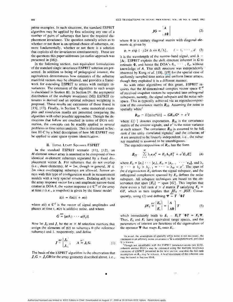
gorithm is due in part to its applicability to arbitrary, but known (i.e., calibrated) antenna arrays. Its principal dis- advantages are the heavy computational and memory re- quirements inherent in the array calibration and spectral search procedures. For the special case of a uniform linear array (ULA) of identical sensors, however, the resulting array manifold has a simple analytical form that can be exploited to mitigate these requirements (e.g., the root- MUSIC procedure [ 2 ] , [ 1 11 or the algorithm of Tufts and Kumaresan [22]). The ESPRIT algorithm was among the first to demonstrate that similar computational savings could also be achieved for more general antenna array configurations. In particular, ESPRIT requires no calibra- tion step, and parameter estimates are obtained directly via two well-conditioned eigenproblems of size 2d and d. However, ESPRIT cannot optimally exploit additional structure in the sensor array beyond a single displacement invariance. As a result, for many arrays there exist several possible choices of subarray pairs that satisfy the dis- placement invariance requirement, and there is no general criterion for choosing one pair over another [15]. Some possible ULA subarray configurations are shown in Fig. 1 . Note that although only a single displacement invari- ance is being used, for overlapping subarrays more of the underlying structure of the array is being exploited.

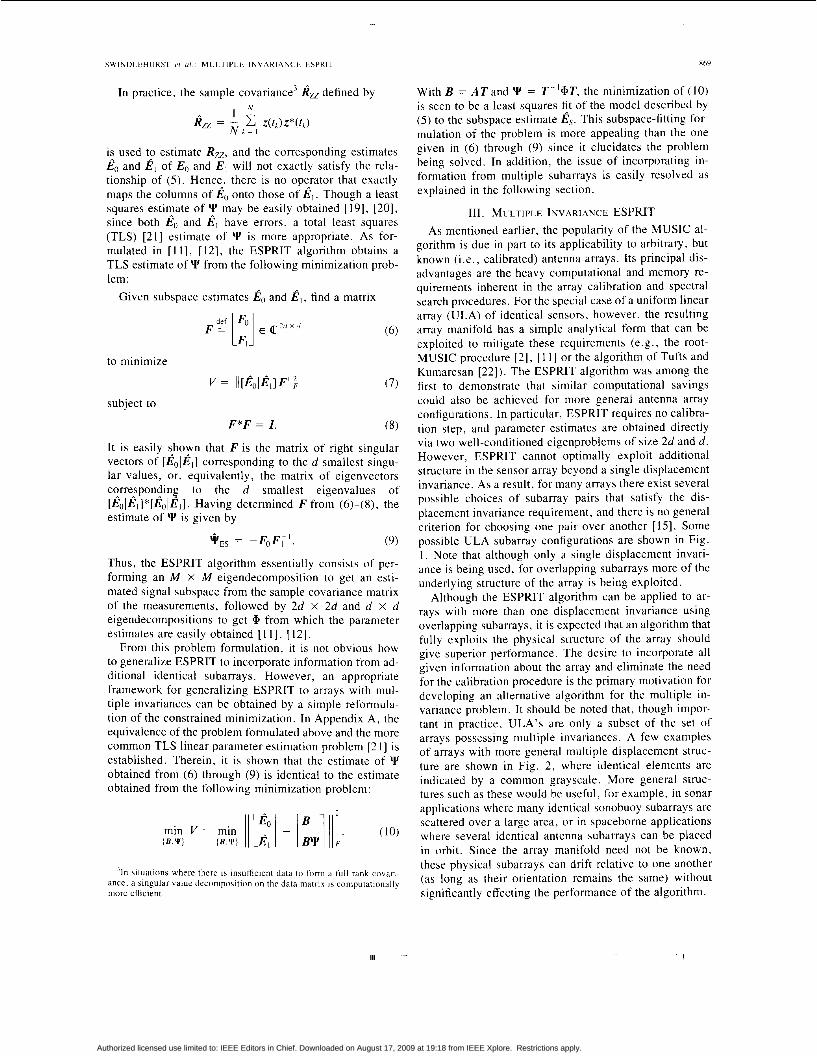
Although the ESPRIT algorithm can be applied to ar- rays with more than one displacement invariance using overlapping subarrays, it is expected that an algorithm that fully exploits the physical structure of the array should give superior performance. The desire to incorporate all given information about the array and eliminate the need for the calibration procedure is the primary motivation for developing an alternative algorithm for the multiple in- variance problem. It should be noted that, though impor- tant in practice, ULA's are only a subset of the set of arrays possessing multiple invariances. A few examples of arrays with more general multiple displacement struc- ture are shown in Fig. 2, where identical elements are indicated by a common grayscale. More general struc- tures such as these would be useful, for example, in sonar applications where many identical sonobuoy subarrays are scattered over a large area, or in spaceborne applications where several identical antenna subarrays can be placed in orbit. Since the array manifold need not be known, these physical subarrays can drift relative to one another (as long as their orientation remains the same) without significantly effecting the performance of the algorithm.

111 - I

Authorized licensed use limited to: IEEE Editors in Chief. Downloaded on August 17, 2009 at 19:18 from IEEE Xplore. Restrictions apply.

870 IEEE TRANSACTIONS ON SIGNAL PROCESSING, VOL. 40, NO. 4. APRIL 1992

where M is a matrix derived from the data, and G(q) de- scribes the parameterization of the array response which T attempts to map onto M . Algorithms other than ESPRIT that belong to this class include MUSIC, beamforming, and the deterministic maximum likelihood approach [23].

Subarray 2

f ............ 3

Subarray 1

(a) Referring back to (lo), it is seen that for ESPRIT

Subarray 2

2 ............ With this choice for M and G, it is shown in [ 151 that the following parameter vector q leads to a uniquely defined solution to (1 1):

I Subarray 1

(b)

q = [vec (zX)~, vec p l , . . . . Pd, e , , . . . . e,] Subarray 2

(13) ............ - Subarray 1

(c) Fig. I . Several ULA subarray choices for ESPRIT. (a) Maximum overlap

(b) Interleaved. (c) Mixed.

r. - . ._____._______ , ~_...._______..._., r_______..........,

! @ 0 0; , I 0 I O i Q 0 0 : .........................................................

A2 *

where 8, is the DOA of the ith source, pI is the magnitude4 of the ith diagonal element of a, and A are, respec- tively, the real and imaginary parts of A , vec ( * ) is the column stacking operator, and f = [O , , - I ) I Z] picks out all but the first row of the matrix to its right. This for- mulation of the problem provides the framework for the most natural extension of ESPRIT to the case where the sensor array is composed of more than two identical sub- arrays. The subspace estimates from additional subarrays are stacked columnwise in M , while the model corre- sponding to each additional subarray is stacked column- wise in G(q).

To make this more precise, assume the array is com- posed of p identical subarrays of m sensors, each with its own displacement vector AI relative to the reference sub- array. The displacement vectors are assumed to be collin- ear. As before, the total number of sensors M need not be equal to mp since overlapping subarrays are allowed. In such cases, M < mp. Let J , be the m X M matrix that describes the i th subarray as in ( l) , and define

Thus, analogous to (3, the structure inherent in E , may be described by the following equation: - 1. ] = 1'1; ] T (14)

Fig. 2. Examples of arrays with multiple displacement invariances.

def

The key to extending ESPRIT to more general array JEs structures is the recognition that it falls in the recently introduced class of subspace-fitting algorithms [ 171. All

of the following common form:

A$$ ~ I algorithms within this class solve a minimization problem Ep- I

'The ESPRIT algorithm does not constrain the diagonal elements of 0 (1 1) to be on the unit circle. so p , . . . . . p,, are implicitly parameters in the min V = min 11M - G(q)Tllf.

11. T ?. T minimization.

Authorized licensed use limited to: IEEE Editors in Chief. Downloaded on August 17, 2009 at 19:18 from IEEE Xplore. Restrictions apply.

SWINDLEHURST er a / . : MULTIPLE INVARIANCE ESPRIT

V =

87 I

[ j W'l2 - L:' A @ ] T . (15)

E p - I ' F

def where 6, = I A, I / 1 A 1 . The MI ESPRIT problem can now be stated as follows:

Given p subspace estimates Eo, E, , ', find a matrix A E C m x d , a matrix T E C d x d , and a di- agonal matrix ip E cd d to minimize

* . , Ep - , E (r:

Note that the displacements { A i } , i = 1, . * , p - 1 , are not necessarily of equal magnitude. Also note that a weighting matrix W1/2 > 0 not appearing in (10) has been included in the cost function V for reasons given in the next section. For the special case of uniformly spaced subarrays, we have Ai = i A l , and consequently 2ii = i. In this special case, the cost function becomes

In the limiting case of a U L A , p is the number of sensors andm = 1.

For ease of notation, (15) is rewritten in the following compact form:

V = llEw - B%)Ii

Ew = [Eo wI/21El wl/21 . . . lEpp W"?]

(16) where the quantities in (16) are defined either as

- def

- def

def ip = [T1+T1ip6'TI * * * lip'" 'TI

B = A , (17) or as

- Ew del = [WT/2Ei(WT/2&Tl . . . (WT/'Er ] P - I

- del 9 = [AT(@AT(@AT( . . . /@b LAT] der

B = TT. (18) As explained shortly, the particular choice of definition is dictated by the desire for a minimal parameterization. Note that the cost function in (16) is separable in the pa- rameter B , and hence B can be solved for directly in terms of the remaining parameters. Setting dV/dB = 0 gives

_ - B = Ew@'* (19)

-+ d i f - where + - [ipip*Ip1%.

With the expression for B given in (19) substituted into (16), the MI-ESPRIT problem (1 5 ) may be reformulated

as

where

(21)

(22)

de f r(q) = vec (E,P&)

def - - P&* = z - ip*[ipip*]-'..

In the general case, the parameter vector q for MI ES- PRIT is defined as in (13), with the exception that A may be replaced by T if the definitions in (17) are used instead of those in (1 8). The choice of which set of definitions to use is dictated by the dimension of q. For the definitions in (17), q E IRZd2, while for those in (1 8), q E WZmd. Con- sequently, if m > d , the definitions in (17) are used, and vice versa. For notational convenience, define m' = min { m , d } , so that in either case tl E IR2m'd.

It is clear from (3) that for DOA estimation problems, the diagonal elements of CP lie on the unit circle (i.e., p, = 1). In such cases, the dimension of the parameter space may be further reduced by eliminating p I , i = 1 , * * , d , from the parameter vector q. Doing so explicitly incor- porates a unitary constraint on the diagonal matrix ip in the minimization of (20).5 However, for many time series applications (e.g., parameter estimation of damped ex- ponentials, system identification, etc.) the unit-norm con- straint does not apply, and the magnitude parameters must be retained in q. To maintain generality in the discusssion that follows, these terms will be included in q.

A. Algorithm Implementation The minimization of V over all q E IR2m'd is a nonlinear,

computationally complex problem, and there exists no easily formulated solution as in the single invariance case. However, using a search technique to achieve dV/dq = 0 is not a serious drawback since the single invariance version of ESPRIT can be applied to provide an excellent initial estimate of q with minimal computational cost. If the sensor array consists of equispaced subarrays, a max- imum overlap configuration where To = [ J i . . * J;-2lT

and 5, = [ J : . . - J ; _ I ] T can be used. For the general case of unequal subarray separation, any suitable invari- ance can be employed by ESPRIT.

One of the most popular and effective algorithms for solving nonlinear least squares problems is Newton's method [24], [25] . The method is based on a second-order expansion of the criterion function about the current pa- rameter estimates, with the step in parameter space taken so as to achieve the local extremum of the approximating

'It IS interesting to note that while eliminating the magnitude terms from q results in a computationally simpler solution f o r p > 2 , whenp = 2 (as for ESPRIT) computational advantage is achieved by retaining them. This is due to the fact that the TLS algorithm of [ 121 cannot efficiently constrain the eigenvalues of Y,, to lie on the unit circle.

111 I

Authorized licensed use limited to: IEEE Editors in Chief. Downloaded on August 17, 2009 at 19:18 from IEEE Xplore. Restrictions apply.

872 IEEE TRANSACTIONS ON SIGNAL PROCESSING. VOL. 40, NO. 4. APRIL 1992

quadratic surface. The Newton iteration can be written as

where pk is a step length (nominally 1) and Hk is the Hes- sian matrix at the kth iteration. The 0th element of Hk is defined as

where 17; and v j are, respectively, the ith and j t h elements of q. The derivatives aV/av i are given by

av 8% - = 2 Re { r T r }

def where r, = ar/aqi . Although the Newton algorithm achieves quadratic convergence when given a sufficiently accurate initial estimate, it requires computation of both first and second derivatives of the cost function. Since in the noise-free case the global minimum of V occurs when llrll = 0 identically, it is expected that in the noisy case, llrll will be reasonably small in the vicinity of the solu- tion. This fact, coupled with the generally high quality of the initial ESPRIT estimate, motivates the following ap- proximation to the second gradient:

{Hk}i j = 2 Re (r;rj + rgr) = 2 Re {r:r,} (24) where

a2r r.. = - " all; a17;

Approximating the elements of the Hessian Hk in (23) by using the expression (24) leads to the so-called Gauss- Newton method [24] , [26]. While maintaining quadratic convergence near the global minimum, the Gauss-New- ton method requires only first derivatives, and is guaran- teed to be a descent method since the approximate Hes- sian is positive semidefinite. Efficient implementations of this method for the type of separable, nonlinear least squares estimation problem considered here can be found in [27]-[30].

The derivatives ri may be computed by first noting that

r; = vec {E,(P$*&.*~' + 5'*5,~$*)) where 4'; = a+/avi. Expressions for the derivatives 3; using the definition of q in (13) are given below. In these expressions, X = T if m I d , X = AT if m < d , X,, is the klth element of X, Zk, is a matrix with 1 in the klth position and zeros elsewhere, and A , = / A , I :

- def -

der

1) vi = Re {&/}

2) 17; = Im

- +; = -[Z k / 1 +Zk/I +*'Zk/l . . . I+*"- IZk/]

+i = - j [Zk/I+lk/(+*2Zk/( * * p*"- 'Zk/] -

3 ) Ti = Pk

1 - a; = -- [o~zkk+x~62z~~+*2x( * . p - 1 zk,+*p-'Xl Pk

4 ) vi = 0 k - ai = - ( j 2 T A , cos e,/x)

* [O(zkk+x~6Zzkk~*~X( . . . IS,,- ,Zkk+*+XI. The derivatives of r are arranged so that ?I def -

- rq.k atl q = q ( k )

is an mpd x 2m'd matrix, and HL = rT.krq,k is the expres- sion for the approximate Hessian.

The Gauss-Newton implementation of the MI ESPRIT algorithm then proceeds as follows:

1) Using the ESPRIT algorithm, obtain initial esti- mates of e , , *

2 ) If m 1 d , set X = T ; otherwise, set X = AT. Form the initial parameter vector q(0) as

, e,/, PI, , PO, A and T .

q(0) = [vec (zX)~, vec (I-%)', p , , * ,

Pd3 01, * * 3 Odl 3) Compute the quantities 5, r , T , , ~ , as defined above. 4 ) Update q(k + 1) = q ( k ) + pk(r:,krq,k)p'

5 ) Evaluate IIaV/aqII, and if it is smaller than some prespecified tolerance, terminate the iterations; if not, re- peat steps 3-5.

The bulk of the computation in the above algorithm oc- curs in forming the approximate Hessian and in taking its inverse at each update. For typical values of d , however, these computations are considerably less costjy than the initial eigendecomposition needed to obtain Es. In addi- tion, simulation results indicate that only one or two it- erations are required to achieve a solution sufficiently close to the global minimum.

In extremely difficult cases (when the initial estimate is severely degraded due to poor SNR or a small number of snapshots), it is often helpful to employ the Levenberg- Marquardt approach (see, for example, [24] , [25]) and regularize the problem by adding a scaled identity matrix to the approximate Hessian. As the value of the criterion function decreases and the minimum is approached, the magnitude of the additive term is decreased to improve convergence speed. However, for most cases of interest, this type of regularization is not necessary and the above algorithm can be implemented as given. In Section V , simulation results using the above algorithm are presented for several cases, and the convergence and rms estimation error of the estimates are examined.

&r(q(k)) .

B. Bounds on the Number of Sources An interesting issue that arises when exploiting multi-

ple invariances is that of determining the maximum num- ber of sources d,,, that can be detected. It is clear that

Authorized licensed use limited to: IEEE Editors in Chief. Downloaded on August 17, 2009 at 19:18 from IEEE Xplore. Restrictions apply.

SWINDLEHURST er a l . : MULTIPLE INVARIANCE ESPRIT 873

d,,, 5 M - 1 5 mp - 1 when R,, is full rank, where p is the number of subarrays, m the number of sensors per subarray, and M is the total number of sensors as before. For MUSIC, d,,, = M - 1, while for ESPRIT ( p = 2) the upper bound is d,,, = m . Though d,,,, for p > 2 is difficult to obtain, it is relatively easy to obtain a least upper bound on d for some special array geometries. If the sensor array consists of equispaced subarrays, sub- space estimates from two overlapping subarrays can be defined as follows:

Both Eo and El have dimension m ( p - 1) X d and, in the absence of noise, a d X d matrix Y = T p l @ T would exist satisfying E , = EoY. However if d > m ( p - l ) , this system of equations is underdetermined and there may be solutions other than Y. Thus, with this particular subarray configuration, a maximum of min { m ( p - l ) , M - 1 ) sources can be uniquely resolved. When solving the mul- tiple invariance problem, additional subarray structure is exploited and consequently the maximum number of uniquely resolvable sources will be at least as large as for the maximum overlap configuration. Consequently, for sensor arrays with equispaced subarrays

min { m ( p - l ) , M - 1) 5 d,,, 5 M - 1.

It is assumed in the above discussion that the signal covariance is full rank, i.e., that there are no coherent sources present. As shown in [15], coherent emitters can- not be identified using the single invariance ESPRIT pa- rameterization that was assumed in obtaining I. How- ever, if the array is composed of multiple equispaced identical subarrays, spatial smoothing ideas [3 I], 1321 may be applied under certain conditions to identify coherent emitters. For this special case of uniformly spaced subar- rays, the following least upper bound on d can be derived:

(25)

This expression holds regardless of the coherency struc- ture of the signals. More optimistic bounds are possible under certain assumptions on the structure of Rss. As be- fore, the bound in (25) also applies to the MI ESPRIT algorithm since it exploits additional subarray structure.

To use MI ESPRIT when coherent emitters are present and equispaced subarrays are employed, the ESPRIT al- gorithm is first applied with spatial smoothing to obtain initial DOA estimates. Then MI ESPRIT is implemented as before, except that the matrix T is now d x d ' , where d' is the dimension of the signal subspace.6

min {m, p - 1) 5 d,,,,.

C. A System Ident$cation Example As mentioned earlier, MI ESPRIT can be applied to the

problem of identifying parameters of linear time-invariant systems described by the state space model:

xk+ I = AX, f BUk

y, = C X ~ + D u ~ (26)

where xk is the state of the linear system at time k , uk is the input to the linear system, and y, is the observed out- put. The objective is to estimate the system matrices A , B , c, and D from the input and output data sequences uk and y,, respectively. Naturally, since the states them- selves are not observed, the system matrices are identifi- able only to within an arbitrary nonsingular state trans- formation.

Following the notation developed by De Moor et al. 1331, 1341 it can be shown that

YU' = rxul (27)

where

1 p Y k + l . . . Y k + j - l

1 y k + 2 ' ' ' Y k + j

. . . . . . . . . . . . Y k + i - l Y k + i . * * Y k + I ' f J - 2 '

r = rk; 1 x = IXk X k + l . . * X k t j - I I (28)

U is a block Hankel matrix constructed in exactly the same fashion as Y , and U' is a matrix satisfying UU' = 0. With appropriately chosen values for the block dimen- sions i andj , r will span the column space of the matrix YU I. For purposes of this discussion, YU ' is assumed to be full rank n , a condition that can be guaranteed by proper experiment design.

The relevance of MI ESPRIT to this problem can be deduced by noting that the observability matrix r pos- sesses the same type of multiple shift structure present in the model of (14). To see how this structure might be exploited, define the singular value decomposition of Y U I

YU' = PZQT

and note that there exists a full rank n x n matrix T such that

'A method for determining d and d' is described in 130)

in

P, = TT

Authorized licensed use limited to: IEEE Editors in Chief. Downloaded on August 17, 2009 at 19:18 from IEEE Xplore. Restrictions apply.

874 IEEE TRANSACTIONS ON SIGNAL PROCESSING, VOL. 40, NO. 4, APRIL 1992

where P, is the matrix containing the first n left singular vectors. Expanding this equation further, we obtain

In the presence of additive measurement noise, (29) will of course not hold, and an estimation procedure is re- quired. Several procedures have been proposed [ 181, [33], [34] to exploit the structure of (29), but each relies on only a single overlapping shift invariance in r. To make better use of the structure inherent in r and Ps, the MI ESPRIT algorithm may be used to estimate A and C from 'the following minimization problem:

7

. (30)

F

The matrices B and D are obtained by solving a set of linear equations involving the estimates of A and C [33].

The minimization of (30) can be implemented in ex- actly the fashion described in the previous section, i.e., initial estimates obtained using an algorithm similar to ESPRIT are refined using a simple gradient search. Since the system matrices may only be determined to within an arbitrary state transformation T , to ensure the identifi- ability of the above parameterization one may wish to solve for T as in (18) and (19), and assume some type of structure for the state dynamics matrix A . For example, A could be parameterized as a diagonal matrix or as a matrix with some particular canonical form. This ap- proach has the advantage of allowing one to constrain the estimated system to conform to prior information avail- able about the true system; e.g., an overdamped (A is di- agonal and real) or critically damped (A is diagonal and unitary) system estimate may be desired.

IV. ASYMPTOTIC ANALYSIS As outlined in the previous section, MI ESPRIT be-

longs to the class of subspace-fitting algorithms described by ( 1 1). In [ 171, an asymptotic analysis is carried out for the special case of (11) where M = E, W"', and in [ 151 this analysis is applied to the ESPRIT param- eterization of (12). Using a similar analysis methodology, the asymptotic distribution of the MI ESPRIT estimates can also be derived [35].

First, the uniqueness and consistency of the MI ES- PRIT parameter estimates is established. In [15] it is

shown that, with q defined as in (13), the single invari- ance ESPRIT problem is uniquely parameterized and that consistent parameter estimates are realized if

1) the subarray manifold A is unambiguous, 2) one of the rows of A is fixed, 3) A < h / 2 , 4) Rss is full rank, and 5) d I m.

For the multiple invariance problem, it is clear that conditions 1 and 2 must still hold. The only change nec- essary in condition 3 is that A be replaced by A , . In Sec- tion 111-B, it was shown that for equispaced subarrays, condition 5 could be replaced by the bound d I min { m( p - I ) , M - 1 } when Rss is full rank. For coherent sources or arbitrarily spaced subarrays, the more conservative least upper bound d I min { m , p - l} is sufficient. Using the arguments of Section 111-B and the proof given in [ 151 for the single invariance case, it is straightforward to show that the following conditions are then sufficient to guar- antee the uniqueness and consistency of the MI ESPRIT parameter estimates:

1) the subarray manifold A is unambiguous, 2) one of the rows of A is fixed, 3) A , < h / 2 , and 4) one of the following is satisfied:

a) Rss is full rank and d I min { m ( p - I), M -

b) d I min ( m , p - 1). l } for equispaced subarrays, or

It should be emphasized that the above conditions are sufficient, and not necessary in all cases. There are, of course, many scenarios for which MI ESPRIT will yield consistent estimates even though some or all of the con- ditions are not satisfied.

When a unique and consistent solution is guaranteed, the asymptotic distribution of the estimate 4 obtained from the MI ESPRIT algorithm is given by the following theo- rem, the proof of which follows immediately from the re- sults in [15], [17].

Theorem IV. 1: Assume that {z(t)] are i.i.d. Gaussian random vectors. For fi obtained from minimizing V(q) de- jined in (15), the estimation error &(4 - qo) is asymp- totically Gaussian distributed with e r o mean and vari- ance C(W) = VI' - 'QV" ', where V and Q are de$ned in Appendix B.

A . Optimal Subspace Weighting A key result of the analysis in [17] is the development

of the weighEed subspace fitting (WSF) technique, for which M = E,y WL& in (1 1) and

where e2 is a consistent estimate of the noise variance and As are the signal eigenvalues of the sample covariance R , as in (4). The weighting WAi: is optimal in the sense that no other choice for W leads to a lower asymptotic

Authorized licensed use limited to: IEEE Editors in Chief. Downloaded on August 17, 2009 at 19:18 from IEEE Xplore. Restrictions apply.

SWINDLEHURST er al.: MULTIPLE INVARIANCE ESPRIT 875

variance for the parameter estimates. Further work has shown that the asymptotic variance of the WSF algorithm in fact achieves the Cramer-Rao bound (CRB) under the assumption of Gaussian emitter signals [36] and for more general array manifold parameterizations that include ele- ments of the array response vectors themselves.

Usin the results of [36], it can be shown that if M =

guaranteed for W = WO,, provided that J J T = Z. For MI ESPRIT, this condition on J signifies that there are no overlapping subarrays. The loss of efficiency for the over- lapping case is a reflection of the fact that additional struc- ture in the sensor array is being assumed, but not opti- mally exploited by the algorithm. Naturally, in cases where a nonoverlapping subarray configuration that uses all of the array elements does not exist (such as for the two arrays at the bottom of Fig. 2), an overlapping struc- ture is clearly preferred over deleting some of the sensors. Although the optimality of WO,, has not been analytically established for cases involving overlapping subarrays, in numerical evaluation of C( W) for several scenarios, it has been observed that C(Z) > C(WopT).

J& W 1 7 2 (as in MI ESPRIT), asymptotic efficiency is

V . SIMULATION RESULTS In this section, simulation results are presented to il-

lustrate the performance of the MI ESPRIT algorithm. The algorithm is compared with MUSIC, root-MUSIC, and ESPRIT, and is shown to have superior performance in terms of resolution and RMS error of the parameter esti- mates. For these simulations, the emitter signals were generated as constant amplitude planewaves with random phase, uniformly distributed on [0, 2 ~ 1 . The sensor array elements were assumed to have unity gain in the direction of the impinging signals, and in all cases it was assumed that the detection problem was correctly solved; i.e., a signal subspace of dimension d was always used. It is im- portant to note that the unit-circle constrained parameter- ization was used for all MI ESPRIT results (i.e., the mag- nitude parameters p I , . * . , Pd were not included in q). This constraint has been observed to have little effect for cases in which the sources are uncorrelated, but it does result in significantly smaller estimation errors for the correlated case.

A. Case 1 : ULA and Uncorrelated Sources This example demonstrates that the quality of the DOA

estimates improves as more and more array invariances are exploited, i.e., as more information about the array is incorporated. A uniform linear array with 12 elements separated by X/2 was assumed. The array was split into varying numbers of subarrays, in each case maintaining A = X/2. In all cases, each element appears in one and only one subarray. Maintaining a constant value for A and using nonoverlapping subarrays for MI ESPRIT allows the results for each subarray configuration to be meaning- fully compared. With this constraint, there are five ways of decomposing the 12 element ULA into subarrays. La-

TABLE I S U B A R R A Y G R O ~ ~ P I N G S FOR 12-ELEMENT ULA C A S E S 1 AND 2

_____ ~~

P m Subarray Groups

2 6 3 4 { 1 , 4 , 7 , 10) ( 2 , 5 . 8, 1 1 ) { 3 , 6 , 9 , 12) 4 3 6 2

12 1

( 1 . 3, 5 , 7 , 9, 11) ( 2 , 4 , 6, 8, 10, 12)

{ I , 5 , 9 ) ( 2 . 6. 10) (3 , 7, 11 ) (4 , 8, 12) (1 . 7 ) (2 , 8) (3, 9) (4 , 10) ( 5 , 11) ( 6 , 10) (1 ) ( 2 ) (31 ( 4 ) (51 ( 6 ) ( 7 ) (81 (9) (10) (111 (121

beling the elements of the ULA from 1 to 12 and using braces { } to denote subarray grouping, the subarray con- figurations are given in Table I. As before, p and m rep- resent the number of subarrays and the number of ele- ments per subarray, respectively.

As p increases, more and more information about the sensor array is incorporated into the MI ESPRIT algo- rithm. Whenp = 12, the array manifold is known and the physical structure of the array is being completely ex- ploited. In this case, MI ESPRIT is equivalent to the WSF algorithm. For each subarray grouping, the results of the MI ESPRIT algorithm are compared with the maximum overlap configuration of the single invariance version of ESPRIT; i.e., the two ESPRIT subarrays are formed by grouping together the first p - 1 and last p - 1 mini- subarrays, respectively.

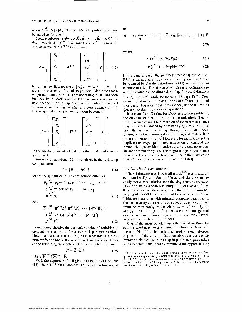
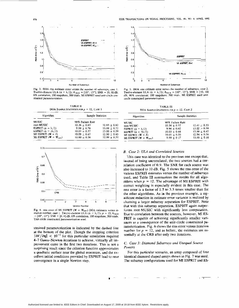
For the specific case considered here, two uncorrelated sources were present at 10" and 13". The separation be- tween the sources was roughly one quarter of a beam- width. The signal-to-noise ratio (SNR) per element for each source was 0 dB, and 100 snapshots were observed from the array for each of the 500 trials. Fig. 3 shows a plot of the rms error of the DOA estimates versus the number of subarrays used for the various versions of ES- PRIT. The relative performance of the algorithms is vir- tually identical for p = 2 and p = 3. As p increases from 4 to 12, the advantage of MI ESPRIT gradually becomes more pronounced, until at p = 12 the improvement in estimation error is roughly 40% over ESPRIT with A = X/2. The advantage of using the correct weighting W = WO,, (see (31)) is also clearly demonstrated. Table I1 summarizes the results of the simulation for the case p =

12, where both MUSIC and root-MUSIC can be applied as well. The numbers given are the sample mean f stan- dard deviation of the estimates. A MUSIC failure was said to occur when the algorithm was unable to resolve two sources within the interval [3", 20'1. It is interesting to note that as indicated in Table 11, using a maximum overlap configuration with A = 3X/2, ESPRIT outper- forms root-MUSIC, and performs nearly as well as opti- mally weighted MI ESPRIT.

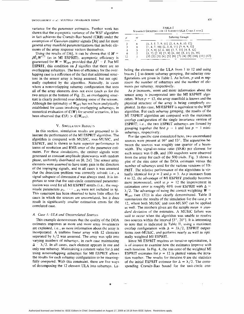
Since MI ESPRIT requires an iterative optimization, it is of interest to examine how the estimates improve with each iteration. In Fig. 4, the rms error of the weighted MI ESPRIT estimates for p = 12 is plotted versus the itera- tion number. The results for iteration 0 are the statistics of the initial ESPRIT estimate for A = X/2. The corre- sponding CramCr-Rao bound for the unit-circle con-

Authorized licensed use limited to: IEEE Editors in Chief. Downloaded on August 17, 2009 at 19:18 from IEEE Xplore. Restrictions apply.

876

21-T----- ' ' 1

. . -

IEEE TRANSACTIONS ON SIGNAL PROCESSING, VOL. 40, NO. 4, APRIL 1992

MI-ESPRIT, W=l. - ESPRIT

MI-ESPRIT, Wopi - 1

\ 2 3 4 6 12

0.4

Number of Subarrays

Fig. 3. DOA rms estimate error versus the number of subarrays, case 1. Twelve-element ULA (A = h/2); &RUE = [ IO" , 13"l: SNR = [O, 01 dB; 0% correlation; 100 snapshots; 500 trials. MI ESPRIT used unit-circle con- strained parameterization.

TABLE I1 DOA SAMPLE STATISTICS FOR^ = 12, CASE 1

Algorithm Sample Statistics

MUSIC 98 % Failure Rate root-MUSIC 10.36 f 0.65 12.63 f 0.62 ESPRIT (A = X / 2 ) 9.98 f 0.78 13.08 rt 0.72 ESPRIT (A = 3X/2) 10.03 f 0.57 13.00 f 0.59 MI ESPRIT (W = I ) 12.90 * 0.65 MI ESPRIT ( W = WO,,) 12.99 & 0.51

10.09 f 0.67 10.00 f 0.56

0.75 I

0.45 1 2 3 4 5 6 7

Iteration Number

Fig. 4. rms error of MI ESPRIT (W = WO,,) DOA estimates versus it- eration number, case 1. Twelve-element ULA (A = X/2); p = 12; = [lo", 13"]; SNR = [O, 01 dB: 0% correlation; 100 snapshots: 500 trials. Unit-circle constrained parameterization used.

strained parameterization is indicated by the dashed line at the bottom of the plot. Though the stopping criterion IldV/dqll < lop5 for this particular simulation required 4-7 Gauss-Newton iterations to achieve, virtually all im- provement came in the first two iterations. This is not a surprising result since the criterion function approximates a quadratic surface near the global minimum, and the ex- cellent initial conditions provided by ESPRIT lead to near convergence in a single Newton step.

1.6 7 I

ESPRIT

MI-ESPRIT, W=l

O 4 I 0.2 I MI-ESPRIT, Wopr

01 I 2 3 4 6 12

Number of Subarrays

Fig. 5. DOA rms estimate error versus the number of subarrays, case 2. Twelve-element ULA (A = h /2 ) ; BTRUE = [ IO" , 13"]; SNR = [ IO, 101 dB; 90% correlation; 100 snapshots; 500 trials. MI ESPRIT used unit- circle constrained parameterization.

TABLE I11 DOA SAMPLE STATISTICS FOR^ = 12, CASE 2

Sample Statistics Algorithm

98% Failure Rate MUSIC root-MUSIC 10.54 f 0.57 12.41 f 0.53 ESPRIT (A = X/2) 9.94 f 0.62 13.02 f 0.58 ESPRIT (A = 3h/2) 10.03 f 0.44 13.00 f 0.47 M1 ESPRIT (W = I ) 12.94 f 0.56

13.00 & 0.16 10.01 f 0.53 9.99 f 0.17 MI ESPRIT ( W = WO,,)

B. Case 2: ULA and Correlated Sources 'i'his case was identical to the previous one except that,

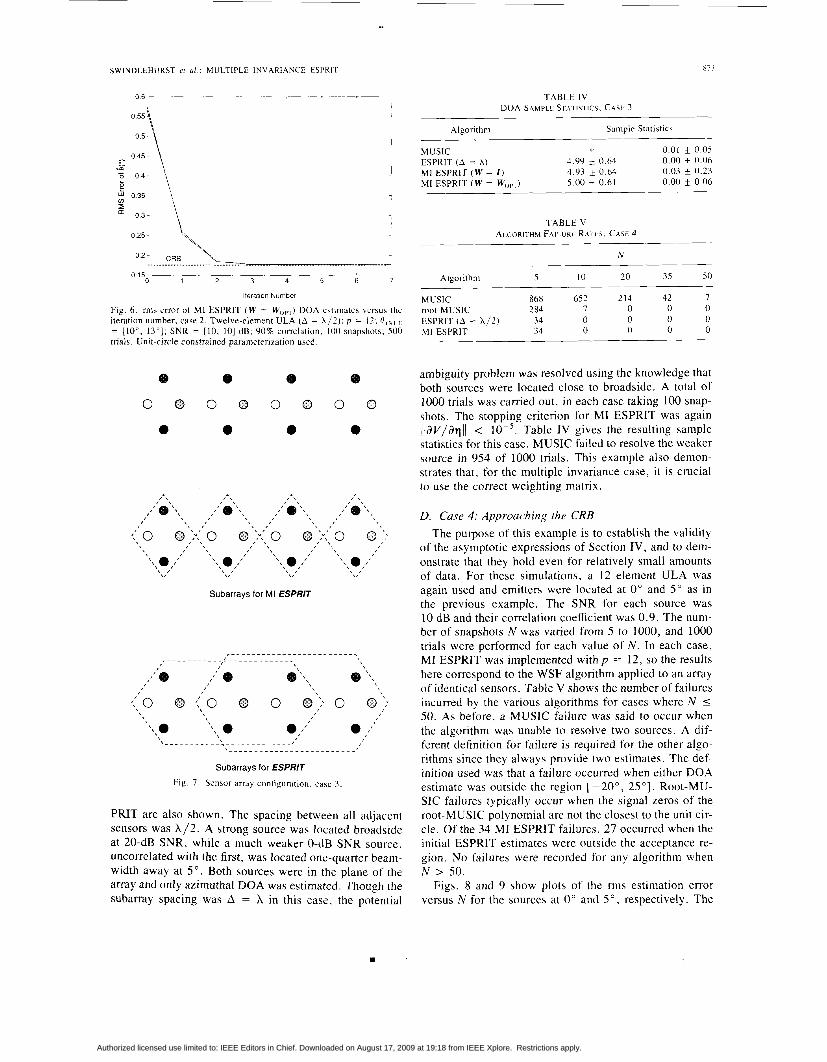
instead of being uncorrelated, the two sources had a cor- relation coefficient of 0.9. The SNR for each source was also increased to 10 dB. Fig. 5 shows the rms error of the various ESPRIT estimates versus the number of subarrays used, and Table I11 summarizes the results for all algo- rithms when p = 12. The advantage of MI ESPRIT with correct weighting is especially evident in this case. The rms error is a factor of 1.5 to 3.5 times smaller than for the other algorithms. As in the previous example, a sig- nificant reduction in estimate error variance is realized by choosing a larger subarray separation for ESPRIT. Note that with this subarray separation, ESPRIT again outper- forms root-MUSIC with significantly less computation. Due to correlation between the sources, however, MI ES- PRIT is capable of achieving significantly smaller vari- ances as a consequence of the unit-circle constrained pa- rameterization. Fig. 6 shows the rms error versus iteration number for p = 12, and as before, the estimates are es- sentially at the CRB after only two iterations.

C. Case 3: Diamond Subarrays and Unequal Source Powers

For this particular scenario, an array composed of four identical diamond shaped arrays shown in Fig. 7 was used. The subarray configurations used for MI ESPRIT and ES-

1

Authorized licensed use limited to: IEEE Editors in Chief. Downloaded on August 17, 2009 at 19:18 from IEEE Xplore. Restrictions apply.

SWINDLLHURST PI U / MULTIPLE I N V A R I A N C E ESPRI r 877

055h I

025,

0 15 l 1 2 3 4 5 6 7

Iteration Number

Fig. 6 . rms error of MI ESPRIT ( W = W,,,,) DOA estimates versus the iteration number, case 2 . Twelve-element ULA (A = X / 2 ) ; p = 12; O , , , , , = (IO", 13"]; SNR = (10, 101 dB; 90% correlation: 100 snapshots; 500 trials. Unit-circle constrained parameterization used.

0 0 0 0 0 0 0 0

Subarrays for MI ESPRlT

Subarrays for ESPRIT

Fig. 7. Sensor array contiguratlon. caw 3

PRIT are also shown. The spacing between all adjacent sensors was h / 2 . A strong source was located broadside at 20-dB SNR, while a much weaker 0-dB SNR source, uncorrelated with the first, was located one-quarter beam- width away at 5". Both sources were in the plane of the array and only azimuthal DOA was estimated. Though the subarray spacing was A = X in this case, the potential

TABLE 1V DOA SAMPLt, STATISI ICS, CASE_ 3

Algorithm Sample Statistics

MUSIC * 0.01 * 0.0s ESPRIT ( A = A) 4.99 0.64 0.00 f 0.06

0.03 k 0.23 MI ESPRIT ( W = I ) MI ESPRIT ( W = W,,,,) 5.00 -t 0.61 0.00 0.06

4.93 & 0.64

TABLE V ALGORITHM FAILLIRF RATtS, C A S E 4

N ~~

Algorithm 5 10 20 35 50 ~~

MUSIC 868 652 214 42 7 root-MUSIC 284 7 0 0 0 ESPRIT ( A = h / 2 ) 34 0 0 0 0 MI ESPRIT 34 0 0 0 0

ambiguity problem was resolved using the knowledge that both sources were located close to broadside. A total of 1000 trials was carried out, in each case taking 100 snap- shots. The stopping criterion for MI ESPRIT was again l/dV/dqII < Table IV gives the resulting sample statistics for this case. MUSIC failed to resolve the weaker source in 954 of 1000 trials. This example also demon- strates that, for the multiple invariance case, it is crucial to use the correct weighting matrix.

D. Case 4: Approaching the CRB The purpose of this example is to establish the validity

of the asymptotic expressions of Section IV, and to dem- onstrate that they hold even for relatively small amounts of data. For these simulations, a 12 element ULA was again used and emitters were located at 0" and 5" as in the previous example. The SNR for each source was 10 dB and their correlation coefficient was 0.9. The num- ber of snapshots N was varied from 5 to 1000, and 1000 trials were performed for each value of N . In each case, MI ESPRIT was implemented with p = 12, so the results here correspond to the WSF algorithm applied to an array of identical sensors. Table V shows the number of failures incurred by the various algorithms for cases where N I 50. As before, a MUSIC failure was said to occur when the algorithm was unable to resolve two sources. A dif- ferent definition for failure is required for the other algo- rithms since they always provide two estimates. The def- inition used was that a failure occurred when either DOA estimate was outside the region [-20", 25'1. Root-MU- SIC failures typically occur when the signal zeros of the root-MUSIC polynomial are not the closest to the unit cir- cle. Of the 34 MI ESPRIT failures, 27 occurred when the initial ESPRIT estimates were outside the acceptance re- gion. No failures were recorded for any algorithm when N > 50.

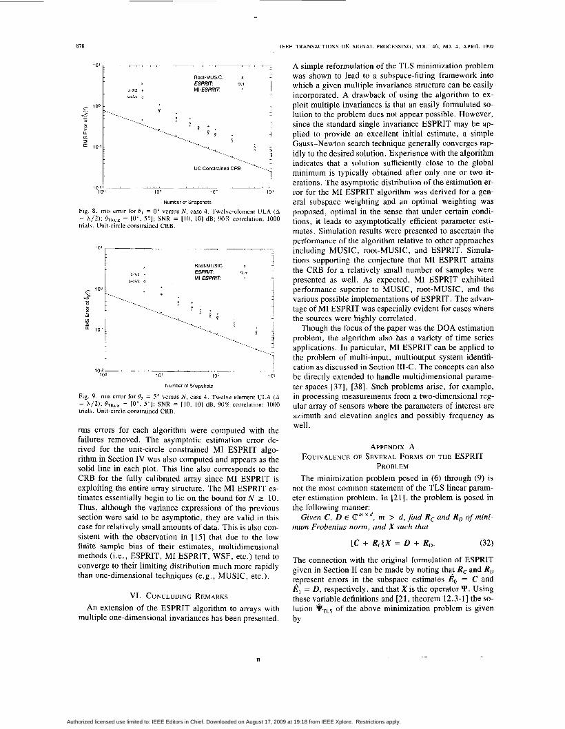
Figs. 8 and 9 show plots of the rms estimation error versus N for the sources at 0" and 5 " . respectively. The

m - 1

Authorized licensed use limited to: IEEE Editors in Chief. Downloaded on August 17, 2009 at 19:18 from IEEE Xplore. Restrictions apply.

878

ESPRIT A=N2 + MI-ESPRIT

b 3 N 2 o

IEEE TRANSACTIONS ON SlGNAL PROCESSING, VOL. 40, NO. 4, APRIL 1992

UC Constrained CRB

IO' 102 103 10-2

100

Number of Snapshots

Fig. 8. rms error for 0 , = 0" versus N , case 4. Twelve-element ULA (A = h / 2 ) ; @TRUE = [ O " , 5PI; SNR = [ I O , IO] dB; 90% correlation; 1000 trials. Unit-circle constrained CRB.

A&2 t i b 3 N 2 o

Root-MUSIC X

ESPRIT 0,+ MI- ESPRIT

10~2 ' 100 IO' 102 103

Number of Snapshots

Fig. 9 . rms error for O2 = 5" versus N , case 4. Twelve-element ULA (A = h / 2 ) ; &RUE = [O", 5 " ] ; SNR = [IO, IO] dB; 90% correlation; 1000 trials. Unit-circle constrained CRB.

rms errors for each algorithm were computed with the failures removed. The asymptotic estimation error de- rived for the unit-circle constrained MI ESPRIT algo- rithm in Section IV was also computed and appears as the solid line in each plot. This line also corresponds to the CRB for the fully calibrated array since MI ESPRIT is exploiting the entire array structure. The MI ESPRIT es- timates essentially begin to lie on the bound for N 2 10. Thus, although the variance expressions of the previous section were said to be asymptotic, they are valid in this case for relatively small amounts of data. This is also con- sistent with the observation in [15] that due to the low finite sample bias of their estimates, multidimensional methods (i.e., ESPRIT, MI ESPRIT, WSF, etc.) tend to converge to their limiting distribution much more rapidly than one-dimensional techniques (e.g., MUSIC, etc.).

VI. CONCLUDING REMARKS An extension of the ESPRIT algorithm to arrays with

multiple one-dimensional invariances has been presented.

A simple reformulation of the TLS minimization problem was shown to lead to a subspace-fitting framework into which a given multiple invariance structure can be easily incorporated. A drawback of using the algorithm to ex- ploit multiple invariances is that an easily formulated SO-

lution to the problem does not appear possible. However, since the standard single invariance ESPRIT may be ap- plied to provide an excellent initial estimate, a simple Gauss-Newton search technique generally converges rap- idly to the desired solution. Experience with the algorithm indicates that a solution sufficiently close to the global minimum is typically obtained after only one or two it- erations. The asymptotic distribution of the estimation er- ror for the MI ESPRIT algorithm was derived for a gen- eral subspace weighting and an optimal weighting was proposed, optimal in the sense that under certain condi- tions, it leads to asymptotically efficient parameter esti- mates. Simulation results were presented to ascertain the performance of the algorithm relative to other approaches including MUSIC, root-MUSIC, and ESPRIT. Simula- tions supporting the conjecture that MI ESPRIT attains the CRB for a relatively small number of samples were presented as well. As expected, MI ESPRIT exhibited performance superior to MUSIC, root-MUSIC, and the various possible implementations of ESPRIT. The advan- tage of MI ESPRIT was especially evident for cases where the sources were highly correlated.

Though the focus of the paper was the DOA estimation problem, the algorithm also has a variety of time series applications. In particular, MI ESPRIT can be applied to the problem of multi-input, multioutput system identifi- cation as discussed in Section 111-C. The concepts can also be directly extended to handle multidimensional parame- ter spaces [37 ] , [38]. Such problems arise, for example, in processing measurements from a two-dimensional reg- ular array of sensors where the parameters of interest are azimuth and elevation angles and possibly frequency as well.

APPENDIX A EQUIVALENCE OF SEVERAL FORMS OF THE ESPRIT

PROBLEM The minimization problem posed in (6) through (9) is

not the most common statement of the TLS linear param- eter estimation problem. In [21], the problem is posed in the following manner:

Given C, D E C m x d , m > d , find Rc and RD of mini- mum Frobenius norm, and X such that

The connection with the original formulation of ESPRIT given in Section I1 can be made by noting tha! Rc and RD represent errors in the subspace estimates Eo = C and 8, = D , respectively, and that X is the operator Y. Using these vyiable definitions and [21, theorem 12.3-11 the so- lution YTLS of the above minimization problem is given by

n

Authorized licensed use limited to: IEEE Editors in Chief. Downloaded on August 17, 2009 at 19:18 from IEEE Xplore. Restrictions apply.

SWINDLEHURST e! a / . : MULTIPLE INVARIANCE ESPRIT 879

(33) The estimate of Y is thus given by EM* E; l , and the or- thogonality relation

E ; ~ + E ; ~ = o (38)

now easily establishes the equivalence Y = YES =

is the matrix of right singular vectors obtained from the following singular value decomposition:

E = [$lfil] = mV*.

In [ l 11, [12] it is shown that the ESPRIT estimate of Y for the formulation of the problem in (6) through (9) is given by YES = -E12EG1, where

- E 1 2 E 2 2 ' .

APPENDIX B THE ASYMPTOTIC VARIANCE OF MI ESPRIT

From [ 151, the parameter estimation error fi(Q - qo) is asymptotically Gaussian distributed with zero mean and variance C( W ) = 'QW - I , where the ik th elements of ,, and Q are given by

- def

(39) -

(34)

- - Qlk = 2a2 Re [tr {G,*Pk J J T P & G , r ~ } ] (40) is the eigendecomposition of E*E. The equivalence of the - - right singular vectors of E and the eige;vectors of E *E establishes the equivalence of YTLs and YES.

through (9), and that obtained from (10) will now be es- tablished. Using standard properties of the trace operator, the minimization of (7) can be rewritten as

V,'k = -2 Re [tr { G ~ P ~ G , T v } I E*E = i"" En] A ["" E12]*

E21 E22 E21 E22

with

The equivalence of the operator Y obtained from (6) rV = G + J E ~ WE; J ~ G ? * (41)

(42)

G' = (G*G)-~G* (43)

rQ = GtJEsWAsAp2WE;JTGt*

min J = min tr {E*EP,) (35) A = A5 - a21 (44) F F

where PF = F[F*F]- 'F* = F F * is the projection onto the (full rank) columns of F. Equation (10) can be written in a similar fashion by solving for B as in (19):

(36) min J = min tr {E:*%P+,} \y \y

where -

Y* = [;d. Thus, the two minimization problems have equivalent forms' since both are minimizations of the same func- tional form over rank d projection matrices in (c 2d 2 d .

obtained from (36) is identical to the ESPRIT estimate YES, begin by defining

To see that the matrix

and note that minimizing (36) will lead to a projection operator satisfying Pi& = PE2. By the orthogonality of the eigenvectors of E*E, Pi& = PE? implies Pip = P E , . Therefore, there exists a nonsingular matrix T such that

- _

(37)

'There is, however, a subtle d i k r e n c e in the constraints. Mathemati- cally speaking, the set of matrices of the form q* is a subset of all fu l l - rank matrices in C """ since full-rank matrices whose upper d x d block

and G, = aG/aq, . The parameter vector q is defined in (13), and all expressions are evaluated using the true pa- rameter vector qo. The vector q has four distinct blocks, and ,, and Q is partitioned accordingly. Note that though the top row of A is not included in the parameterization, it is notationally simpler to first consider all elements of the matrix A as parameters, and afterwards use a selection matrix 1, to neglect the columns and rows corresponding to the top row of A . Define the matrices V and & so that

(45)

The matrices V and & have a four by four block structure VI,, Q,, i , j = 1 , . * . , 4, where each block corresponds to a particular combination of parameters from q, such as

(46)

(47)

-

V = - 2 1 , Re (V)]:, Q = 2 0 ~ 1 ~ Re (&)jf.

v,, * vec (A), vec (A) v12 ++ vec (A), vec (A)

v13 vec (A), [ P I , . . . , P ~ I (48)

vI4 ++ vec (A), [ e , , . * . > e,]. (49)

The other blocks in V and those of Q are obtained in a similar fashion. The selection matrix 1, that selects all rows and columns except those corresponding to the top row of A has the following structure:

(50) 1, = blockdiag [I, * . . , 1, 12dx2d]. L4

2d

is not invertible cannot be converted into the form of Y*.'For the problems considered herein, such an event occurs with probability zero and need not Some definitions are required before giving the expres- be considered further. sions for the blocks of V and &. The projection matrix

111 - 1

Authorized licensed use limited to: IEEE Editors in Chief. Downloaded on August 17, 2009 at 19:18 from IEEE Xplore. Restrictions apply.

880 IEEE TRANSACTIONS ON SIGNAL PROCESSING, VOL. 40, NO. 4, APRIL 1992

Pk is partitioned into m X m blocks

P V l l . . . P V l p

p v p i * p v p p

P& = [ ! *.. ! 1 and similarly, P; JJ‘P; is partitioned into P,,,, i, j = 1 , . . . , p . The matrices of partial derivatives of 4) are de- noted

(51)

+p = diag [exp (j27r A, sin el), . . . , exp (j27r A, sin e,)] (52)

GO = diag [p1j27r A, cos Oi exp (j27r A , sin O,), . * . ,

pJ2n A, cos Od exp (j27r A, sin O d ) ] . (53)

The matrix D will be defined in the following manner:

D = [0,xmlAT12+ATI * * I(p - 1)+p-2AT]T (54)

where it is hereafter assumed that the subarrays are equi- spaced. The extension to arbitrary separations is trivial. Finally, J2 will denote the following d2 X d selection ma- trix:

J 2 = [ZII 122 . . . Zd,lT (55)

where Zl, is a matrix with 1 in the ijth position and zeros elsewhere.

The blocks of V are now given as follows: P P

vII = C C (+r-lr,,wl*) 8 (pV,,f

v 2 2 = vi, v3, = o (D*P;D)~

r = l ~ = l

v23 = j V 1 3

v24 = J v 1 4

where @ denotes the Kronecker product [39], 0 the Schur product (elementwise multiplication) and (D*P&), is the rth m X m block of D*Pk. The blocks of Q are con- structed in exactly the same manner as those of V, except that Tv is replaced with T a , Pv, with P,,, and P & with P; JJ~P;.

REFERENCES

[ I ] G. Bienvenu and L. Kopp, “Principle de la goniometrie passive adap- tive,” in Proc. 7’eme Colloyue GRESIT (Nice, France). 1979, pp. 1061 1- 1061 I O .

121 R. Schmidt, “A signal subspace approach to multiple emitter location and spectral estimation,” Ph.D. dissertation, Stanford University, 1981.

131 A. J. Barabell, J. Capon, D. F. Delong, J. R. Johnson, and K. Senne, “Performance comparison of superresolution array processing algo- rithms,’‘ Tech. Rep. TST-72. Lincoln Lab., M.I .T. , 1984.

[4] M. Kaveh and A. Barabell, “The statistical performance of the MU- SIC and the Minimum-norm algorithms in resolving plane waves in noise,” IEEE Trans. Acoust., Speech, Signal Processing, vol. ASSP- 34, no. 2. pp. 331-341, Apr. 1986.

(51 B. Porat and B. Friedlander, “Analysis of the asymptotic relative efficiency of the MUSIC algorithm,” IEEE Trans. Acoust., Speech, Signal Processing, vol. 36, no. 4 , pp. 532-544, Apr. 1988.

[6] P. Stoica and A. Nehorai, ”MUSIC maximum likelihood and Cra- m6r-Rao bound, ’ ’ IEEE Trans. Acoust. , Speech, Signal Processing. vol. 37, no. 5 , pp. 720-741, May 1989.

[7] B. Friedlander. “A sensitivity analysis of the MUSIC algorithm,” IEEE Trans. Acoust., Speech, Signal Processing, vol. 38, no. 10, pp. 1740-1751, Oct. 1990.

181 A. Swindlehurst, B. Ottersten, and T. Kailath, “An analysis of MU- SIC and Root-MUSIC in the presence of sensor perturbations,” in Proc. 23rd Asilomar Conf. Signals, Sysr. , Comput. (Asilomar. CA),

191 A. Swindlehurst and T. Kailath. “A performance analysis of sub- space-based methods in the presence of model errors-Part I : The MUSIC algorithm,” IEEE Trans. Signal Processing, to be published July 1992.

[ l o ] A. Paulraj, R. Roy, and T . Kailath. “A subspace rotation approach to signal parameter estimation,” Proc. IEEE, pp. 1044-1045, July 1986.

[ I I] R. H. Roy, “ESPRIT-Estimation of signal parameters via rotational invariance techniques,” Ph.D. dissertation, Stanford Univ., 1987.

[ 121 R. Roy and T. Kailath, “ESPRIT-Estimation of signal parameters via rotational invariance techniques,” IEEE Trans. Acoust., Speech, Signul Processing, vol. 37, no. 7, pp. 984-995, July 1989.

[I31 R. Roy, A. Paulraj, and T. Kailath, “Method for estimating signal source locations and signal parameters using an array of signal sensor pairs. U.S. Patent, 4 750 147, June 7, 1988.

(141 B. D. Rao and K. Hari, “Performance analysis of subspace based methods, ’ ’ in Proc. 4th ASSP Spectral Estimation Workshop (Min- neapolis, MN), Aug. 1988, pp. 92-97.

I 151 B . Ottersten. M. Viberg, and T . Kailath, “Performance analysis of the total least squares ESPRIT algorithm,” IEEE Trans. Signal Pro- cessing. vol. 39, no. 5 , pp. 1122-1135. May 1991.

1161 R. Roy, B. Ottersten, L. Swindlehurst, and T . Kailath, “Multiple invariance ESPRIT,” in Proc. 22nd Asilomar Conf. Signals, Syst., Comput. (Asilomar, CA), Nov. 1988, pp. 583-587.

[17] M. Viberg and B. Ottersten, “Sensor array processing based on sub- space fitting.” IEEE Trans. Signal Processing, vol. 39. no. 5 , pp. 1110-1121, May 1991.

1181 S . Y . Kung, “A new identification and model reduction algorithm via singular value decomposition,” in Twelfth Asilomar Conf. Circuits, S j s t . , Comput. (Asilomar, CA), Nov. 1978, pp. 705-714.

[19] S . Y. Kung. C . K. Lo, and R. Foka, “A Toeplitz approximation approach to coherent source direction finding,” in Proc. ICASSP 86 (Tokyo. Japan), 1986.

1201 R. Roy, A. Paulraj, and T. Kailath, ”ESPRIT-a subspace rotation approach to estimation of parameters of cisoids in noise,” IEEE Trans. Acoust., Speech, Signal Processing, vol. 34, no. 4, pp. 1340-1342, Oct. 1986.

[21] G. H. Golub and C . F. Van Loan, Matrix Computations. Baltimore, MD: Johns Hopkins University Press, 1984.

1221 D. Tufts and R. Kumaresan, “Frequency estimation of multiple si- nusoids: Making linear prediction perform like maximum likeli- hood,” Proc. IEEE, vol. 70, pp. 975-990, 1982.

1231 M. Wax. ”Detection and estimation of superimposed signals,” Ph.D. dissertation, Stanford Univ., Stanford, CA, 1985.

1241 P. E. Gill, W. Murray, and M. H. Wright, Practical Optimization. Academic, 1981.

[25] D. G. Luenberger, Linear and Nonlinear Programming. Reading, MA: Wesley, 1984.

[26] J . W. Daniel, The Approximate Minimization of Function&. En- glewood Cliffs, NJ: Prentice-Hall, 1971.

NOV. 1989. pp. 930-934.

n

Authorized licensed use limited to: IEEE Editors in Chief. Downloaded on August 17, 2009 at 19:18 from IEEE Xplore. Restrictions apply.

SWINDLEHURST ef a l . . MULTIPLE INVARIANCE ESPRIT 88 I

G. H. Golub and A. Pereyra. “The differentiation of pseudoinverses and nonlinear least squares problems whose variables separate,” SIAM J . Nurrrer. A d . , vol. 10. pp. 413-432, 1973. L. Kaufman, “A variable projection method for solving separable nonlinear least squares problems,” BIT, vol. 15, pp. 49-57, 1975. A. Ruhe and P. A. Wedin, “Algorithms for separable nonlinear least squares problems,” SIAM Rei , . , vol. 22. pp. 318-327. 1980. M. Viberg, B. Ottersten, and T. Kailath. “Detection and estimation in sensor arrays using weighted subspace fitting,” lEE€ Trans. Sig- nal Processing, vol. 39. no. 1 1 , pp. 2436-2449. Nov. 1991. T. J . Shan, M. Wax. and T. Kailath, “On spatial smoothing for di- rection of arrival estimation of coherent signals.” I € € € Truns. Acousr., Speech, Signal Processing, vol. ASSP-33. no. 4. pp. 806- 811, 1985. T. J . Shan, Array Processing for Coherent Sources, Ph.D. disserta- tion, Stanford Univ., 1986. B. De Moor, “Mathematical concepts and techniques for modelling of static and dynamic systems.” Ph.D. dissertation. Katholieke Uni- versiteit Leuven. Leuven, Belgium, 1988. B. De Moor, M. Moonen, L. Vandenberghe, and J . Vandewalle, “A geometrical approach for the identification of state space models with singular value decomposition,” in Proc. IEEE ICASSP, vol. 4 (New York, NY), 1988. pp. 2244-2247. B. Ottersten, M. Viberg. and T . Kailath. “Analysis of algorithms for sensor arrays with invariance structure,” in Proc. / E € € ICASSP. vol. 5 (Albuquerque, NM), 1990, pp. 2959-2962. B. Ottersten, M. Viberg, and T. Kailath, “Analysis of subspace fit- ting and ML techniques for parameter estimation from sensor array data,” I€€€ Trans. Signal Processing. vol. 40. no. 3. pp. 590-600, Mar. 1992. A. Swindlehurst, R. Roy, and T . Kailath, “Suboptimal subspace fit- ting methods for multidimensional signal parameter estimation.” Proc. SPIEInt . Soc. Opt. E n g . , vol. 1152, pp. 197-208. 1989. A. Swindlehurst and T. Kailath, “2-D parameter estimation using arrays with multidimensional invariance structure.“ in Proc. 23rd Asilomar Cant Signals, Sysr., Comput. (Asilomar. CA), Nov. 1989, pp. 950-954. A. Graham, Kronecker Products und Matrix Calculus u,ith .+plica- tions. Chichester. England: Ellis Horwood, 1981.

A. Lee Swindlehurst (S’83-M’84) was born in Boulder City, NV, in 1960. He received the B.S. (summa cum laude) and M.S. degrees in electrical engineering from Brigham Young University, Provo. UT, in 1985 and 1986, respectively, and the Ph.D. degree in electrical engineering from Stanford University in 1991.

From 1983 to 1984 he wa5 with Eyring Re- search Institute as a Scientific Programmer writ- ing software and documentation for a Minuteman missile simulation system. During 1984-1986. he

was a Research Assistant in the Department of Electrical Engineering at Brigham Young University. His work there included analysis of the effect of integer computations on FFT’s, implementation of a spread-spectrum telephone communication scheme, development of lofargram display nor- malization techniques, and study of empirical Bayes detection methods. He was awarded an Office of Naval Research Graduate Fellowship for 1985- 1988, and during that time was affiliated with the Information Systems Lab- oratory at Stanford University. From 1986 to 1990, he was also employed at ESL, Inc., where he was involved in the design of algorithms and ar- chitectures for a variety of radar and sonar signal processing systems. He is currently an Assistant Professor in the Department of Electrical and Computer Engineering at Brigham Young University. His research inter- ests include sensor array signal processing, detection and estimation the- ory, and system identification and control.

Bjorn Ottersten (S’87-M’89) wa\ born in Stock- holm, Sweden, on July 31, 1961 He received the M S degree in electrical engineering and applied physics from Linkoping University, Linkoping. Sweden, in 1986, and the Ph D degree in elec- trical engineering from Stanford University, Stan- ford, CA, in 1989

From 1984 to 1985. he was employed with Lin- koping University as a Research and Teaching Assistant in the Control Theory Group He was a Visiting Researcher at the Department of Electri-

cal Engineering, Linkoping University, during 1988. In 1990 he was a Postdoctoral Fellow associated with the Information Systems Laboratory, Stanford University, and he is currently an Assistant Professor in the De- partment of Automatic Control at the Royal Institute of Technology, Stock- holm, Sweden. His research interests include stochastic signal processing. sensor array processing, system identification, and time series analysis.

Richard Roy (S’80-M’82) was born in Los An- geles, CA, in 1951. He received the B.S. degree in physics and the B.S. degree in electrical engi- neering in 1972, both from the Massachusetts In- stitute of Technology and the M.S. degree in physics in 1974, the M.S. degree in electrical en- gineering in 1976, and the Ph.D. degree in elec- trical engineering in 1987, all from Stanford Uni- versity.

From 197.5 to 1984 he was employed by ESL, Inc., as a Senior Member of the Technical Staff

involved in research and development of techniques for information pro- cessing applied to intelligence data analysis. From 1983 to 1985, he was also employed as a Member of the Technical Staff of a start-up company in the oil-well services business and was involved in research into and de- velopment of algorithms for real-time signal processing and information extraction from data collected in the oil-well drilling environment. As an Research Scientist for Integrated Systems, Inc., from 1985 to 1987, he was involved in the development of estimation, identification, and adaptive control algorithms for various aerospace applications, including helicopter vibration control and real-time flutter analysis, among others. From 1987 to 1990, he was a Research Associate with the Information Systems Lab- oratory at Stanford University, and a consultant to various firms involved in statistical signal processing and systems analysis, design, and control, which he is now pursuing full time as founder and President of Systems Research Associates, Inc. His current research interests are in the areas of multidimensional statistical signal processing (ESPRIT), system identifi- cation and control, and in the VLSl design and implementation of associ- ated algorithms for real-time applications, especially as they apply to the mobile communication industry.

Thomas Kailath (S’57-M’62-F’70) was edu- cated in Poona, India, and recelved the S M and Sc D. degrees from the Massachusetts Institute of Technology in 1959 and 1961, respectively

From October 1961 to December 1962, he worked with the Jet Propulsion Laboratories, Pas- adena, CA, where he also taught part time at the California Institute of Technology. He joined Stanford University as an Associate Professor of Electncal Engineering in 1963. He has been a Full Professor since 1968, served as Director of the In-

formation Systems Laboratory from 197 1 through 1980, as Associate De- partment Chairman from 1981 to 1987, and currently holds the Hitachi America Professorship in Engineering He has also held short-term ap- pointments at several institutions around the world. He has worked in a number of areas including information theory, communications, compu- tation, control, linear systems, statistical signal processing, stochastic pro- cesses, linear algebra, and operator theory, his recent research interests include array processing, fast algorithms tor nonstationary signal process- ing, and the design of special purpose computing systems. He is the author of Linear Systems (Prentice-Hall, 1980), and Lectures on Wzener and Kal- man Frlrerrng (Springer-Verlag, 198 I )

Dr. Kailath has held Guggenheim, Churchill, and Royal Society fellow- ships, among others, and received awards from the IEEE Information The- ory Society, the IEEE Signal Processing Society, and the American Con- trol Council He served as President of the IEEE Information Theory Society in 1975, and was awarded an honorary doctorate from Linkoping University, Sweden, in I990 He is a Fellow of the Institute of Mathemat- ical Statistics and is a member of the National Academy of Engineering.

111 - 1

Authorized licensed use limited to: IEEE Editors in Chief. Downloaded on August 17, 2009 at 19:18 from IEEE Xplore. Restrictions apply.