ON COMPRESSION - Cory Arcangel's Official Portfolio ... · PDF fileON COMPRESSION Cory Arcangel 2k7 – 2k8 ... circle is centered on the X and Y axis, and has a radius of 1. ... ON

220

ON COMPRESSION

Cory Arcangel2k7 – 2k8

ABSTRACT: JPEGs look the way they do becauseof quantization and their use of the Discrete Co-sine Transform (DCT). The DCT is a techniquefor converting a signal into elementary frequencycomponents. It is widely used in image compres-sion. Here we will go through some examples toexplain how the DCT works. The text is kind ofa summary, and if you want to bring the noise, allthe math is in the end notes.

221 Cory Arcangel

1. LOSSY VS. LOSSLESS

The whole point of digital image compression is to be ableto reconstruct an image without having to send all the data. This is be-cause data, especially in large amounts, is expensive and slow to trans-port. Either over cable lines, phone lines, or wirelessly, it is all slow. Tothis day, the most e!cient and cheapest way to transport large amountsof data is by mailing a hard-drive to the destination, and I don’t meanemailing, I mean the kind of mailing that involves the post o!ce. Socompression is valuable because the less we need to send the cheaperand faster it is. There are two kinds of compression. One is called Lossy,and the other is called Lossless. Lossless compression does not lose anyinformation from the original source. How can this be? Well, let’s saywe wanted to send this: ‘a a a a a a a a a b a’ and we were going to sendit over the phone by voice. As opposed to having to send all the informa-tion by reading out each letter one at a time, we could just tell someone‘9a’s, one b, and one a’ and they would know we meant ‘a a a a a a a a ab a’ and we have saved ourselves a bit of breath. In computer language itmeans we have stored all the information using less space. To generalizea bit, if you have ever opened a ‘zip’ file, your computer has seen ‘9a’s,one b, and one a’ and translated it to ‘a a a a a a a a a b a’. This isLossless compression. On the other hand, Lossy compression actuallyloses data. Lossy compression, therefore, can not be used for text, orany application where all the information must remain intact. It is usedfor images, music, and video. This is because, believe it or not, our eyesand ears are pretty crap, and we don’t usually notice missing bits hereand there. Lossy compression works by getting rid of the informationwhich isn’t so important to us. To generalize a bit again, if we tried tosend ‘a a a a a a a a a b a’ using Lossy compression over the phone,we would just get lazy and say ‘11a’s’. In this article, we are going tofocus on the Discrete Cosine Transform, aka the DCT, a math formulaused in Lossy compression. The reason I’m interested in this Transformis because, when used with quantization, it is what gives JPEGs that‘JPEG look’. By ‘JPEG look’ I mean those crappy compressed blockyimages you need to squint your eyes to understand that are all over theinternet. And in case you haven’t noticed, this look is everywhere elseas well (ads, digital cameras, digital video, etc.) If the ’80s gave us ‘hot’colors and ‘rad’ graphics, and the ’90s gave us slick vector design, then

ON COMPRESSION 222

the 00’s are giving us compressed blocky images.JPEGs are everywhere today because they have become

a standard, or a universally agreed upon set of rules. Today JPEGis a nickname for a file type, but JPEG originated as a shorthand forthe group that proposed the standard, the Joint Photographic ExpertsGroup. This standard was created in Geneva in 1992 when membersof the CCITT and the ISO/IEC (now together known as JPEG) gottogether in Geneva and released the technical document ISO/IEC IS10918-1 / ITU-T Recommendation T.81. This paper recommended‘REQUIREMENTS AND GUIDELINES’ of the ‘DIGITAL COMPRES-SION AND CODING OF CONTINUOUS-TONE STILL IMAGES’.These guidelines, through third party development, eventually becameknown as JPEG files.

2. THE GUY BEHIND THE GUY BEHIND THE GUY

As mentioned earlier, the heart of JPEG is the DCT for-mula, and the DCT relies on cosines. The easiest way to think of cosinesis to imagine yourself walking counterclockwise around a circle. Thiscircle is centered on the X and Y axis, and has a radius of 1. Radiusis the length from the center of the circle to the edge. A cosine of theangle in respect to the positive horizontal axis (aka, the length in ourcase because we are on a unit circle (radius = 1)) is our position on thex axis as we walk around the circle if we started at X = 1. We mustalso remember that the length around a circle with a radius of 1 is 2pi.So, cos(0) is 1, because we haven’t gone anywhere; we are still stand-ing at the beginning, at X = 1, cos(pi) is -1, because we have travelledhalfway around the circle to X = -1, and cos(2pi) is 1, because since wehave travelled all the way around our circle, we have ended up back atthe beginning (Figure 1). It is this cyclical pattern which is useful incompression (Figure 2). To see the DCT in action we will start withthe 1D DCT (Figure 3) formula and use it to compress the input 3,2,1(Figure 4). DCT-based compression has four steps. First the DCT for-mula creates basis functions, then it compares the input data to thosebasis functions, creating what are called DCT coe!cients, then those co-e!cients are quantized, and the last step is decompression, where all thisis done in reverse to recreate our data. The first step of our process canbe seen in Figure 5.1 These are the basis functions for our input, which

223 Cory Arcangel

Figure 1: cosine of 0, pi, and 2pi

Figure 2: Cosine curve of x = 0 to 40

consist of cosine curves of increasing frequency. They can be thoughtof as building blocks. Every combination of 3 digits can be recreatedby adding these blocks together in di!erent proportions. The secondstep in the process is comparing our input to our three basis functionsto generate three DCT coe"cients. Our DCT coe"cients represent howmuch of each basis function is present in our input. In our example, ourthree DCT coe"cients generated by the 1D DTC are 3.46410, 1.41421,

F (u) =N!1X

x=0

w(i)f [x]cos(2x + 1)u!

2N

if i = 0, w =p

1/N , and if i != 0, w =p

2/N

Figure 3: 1D DCT formula. w(i) is a weighting factor fyi

ON COMPRESSION 224

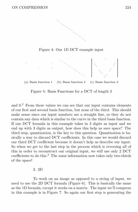
Figure 4: Our 1D DCT example input

(a) Basis function 1 (b) Basis function 2 (c) Basis function 3

Figure 5: Basis Functions for a DCT of length 3

and 0.2 From these values we can see that our input contains elementsof our first and second basis function, but none of the third. This shouldmake sense since our input numbers are a straight line, so they do notcontain any data which is similar to the curve in the third basis function.If our DCT formula in this example takes in 3 digits as input and weend up with 3 digits as output, how does this help us save space? Thethird step, quantization, is the key to this question. Quantization is ba-sically a way to discard DCT coe!cients. In this case we would discardour third DCT coe!cient because it doesn’t help us describe our input.So when we get to the last step in the process which is reversing all ofthis in order to reconstruct our original input, we will use only 2 DCTcoe!cients to do this.3 The same information now takes only two-thirdsof the space!

3. 2D

To work on an image as opposed to a string of input, weneed to use the 2D DCT formula (Figure 6). This is basically the sameas the 1D formula, except it works on a matrix. The input we’ll compressin this example is in Figure 7. So again our first step is generating the

225 Cory Arcangel

F (u, v) =N!1X

x=0

N!1X

y=0

w(i, j)f [x, y]cos(2x + 1)u!

2Ncos

(2y + 1)u!2N

if i or j = 0, w =p

1/N , and if i or j != 0, w =p

2/N

Figure 6: 2D DCT formula

(a) InputImage

2

6

4

255 255 255

0 0 0

0 0 0

3

7

5

(b) Input matrix

Figure 7: Our input matrix

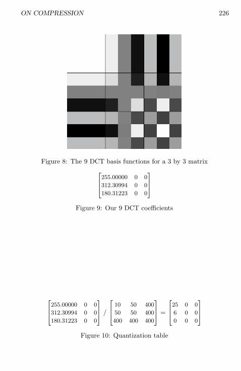
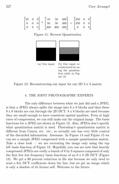
basis functions (Figure 8).4 As in Figure 8, our basis functions with thelower cosine frequencies are on the top left and the basis functions withthe higher cosine frequencies are on the bottom right. Next, we compareour input image to our basis functions to generate our DCT coe!cients.Then, we’re left with 9 DCT coe!cients (Figure 9).5 These numberstell us our input only contains three of our nine basis functions, and onecan see the graphic similarities between the basis functions on the leftside of Figure 8, and our input in Figure 7. All the other basis functionsdo not relate. The third step is quantization. This happens by takingthe DCT coe!cient matrix (Figure 9) and dividing it by a quantizationmatrix, then rounding to the nearest integer. An example matrix is usedin Figure 10. The result, when reversed (Figure 11), gets rid of one ofour DCT coe!cients. If we complete step four by using the quantizedcoe!cients to reconstruct our input, we clearly have quite a big di"er-ence (Figure 12).6 Where did that grey bar come from? EXACTLY!!We have saved a ton of space, because now we only need to transmit‘250, 250, and 7 0s’ to recreate our input, but our image no longer lookshow it was supposed to! This is because we have discarded the highfrequency basis functions, so we can no longer create sharp contrasts.But it’s similar, we get the idea, and this is probably good enough.

ON COMPRESSION 226

Figure 8: The 9 DCT basis functions for a 3 by 3 matrix

2

6

4

255.00000 0 0

312.30994 0 0

180.31223 0 0

3

7

5

Figure 9: Our 9 DCT coe!cients

2

6

4

255.00000 0 0312.30994 0 0

180.31223 0 0

3

7

5/

2

6

4

10 50 40050 50 400

400 400 400

3

7

5=

2

6

4

25 0 06 0 0

0 0 0

3

7

5

Figure 10: Quantization table

227 Cory Arcangel

2

6

4

25 0 0

6 0 00 0 0

3

7

5*

2

6

4

10 50 400

50 50 400400 400 400

3

7

5=

2

6

4

250 0 0

250 0 00 0 0

3

7

5

Figure 11: Reverse Quantization

(a) Our input (b) Our input re-constructed by us-ing the quantiza-tion table in Fig-ure 10

Figure 12: Reconstructing our input for our 2D 3 x 3 matrix

4. THE JOINT PHOTOGRAPHIC EXPERTS

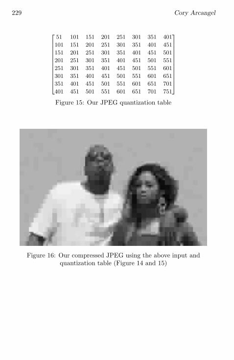
The only di!erence between what we just did and a JPEG,is that a JPEG always splits the image into 8 x 8 blocks and then these8 x 8 blocks are run through the 2D DCT. 8 x 8 blocks are used becausethey are small enough to have consistent spatial qualities. Even at highrates of compression, we can still make out the original image. The basisfunctions for a JPEG are shown in Figure 13. Also, JPEGs don’t specifywhat quantization matrix is used. Photoshop’s quantization matrix isdi!erent from Canon, etc. etc., so actually one has very little controlof the discarded information. Awesome. In Figure 14 and Figure 15 wecan see a sample JPEG compressed with a sample quantization matrix.Take a close look — we are recreating the image only using the topleft basis function of Figure 13. Hopefully you can see now that heavilycompressed JPEGs are really a bunch of 8 by 8 squares composed of onlythe first few low frequency basis functions of an 8 x 8 2D DCT (Figure13). We get a 90 percent reduction in file size because we only need tosend a few DCT coe"cients down the line, but we get an image whichis only a shadow of its former self. Welcome to the future.

ON COMPRESSION 228

Figure 13: Our Basis functions for a JPEG

Figure 14: Our JPEG input

229 Cory Arcangel

2

6

6

6

6

6

6

6

6

6

6

6

4

51 101 151 201 251 301 351 401

101 151 201 251 301 351 401 451

151 201 251 301 351 401 451 501201 251 301 351 401 451 501 551

251 301 351 401 451 501 551 601

301 351 401 451 501 551 601 651351 401 451 501 551 601 651 701

401 451 501 551 601 651 701 751

3

7

7

7

7

7

7

7

7

7

7

7

5

Figure 15: Our JPEG quantization table

Figure 16: Our compressed JPEG using the above input andquantization table (Figure 14 and 15)

ON COMPRESSION 230

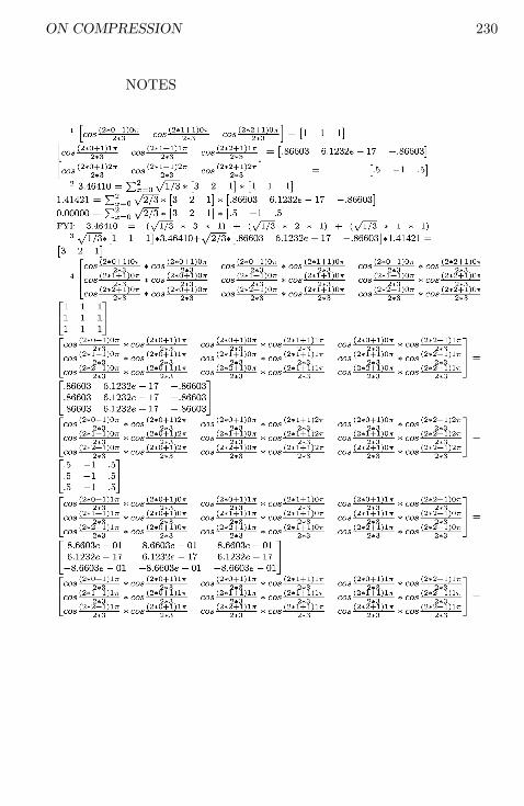
NOTES

231 Cory Arcangel

ON COMPRESSION 232

Special thanks to Danny Comer for helping withthese concepts.