On 1/n neural representation and robustness

On 1/n neural representation and robustness

Josue Nassar⇤

Department of Electrical and Computer EngineeringStony Brook University

[email protected]

Piotr Aleksander Sokol⇤

Department of Neurobiology and BehaviorStony Brook University

[email protected]

SueYeon ChungCenter for Theoretical Neuroscience

Columbia [email protected]

Kenneth D. HarrisUCL Institute of NeurologyUniversity College London

[email protected]

Il Memming ParkDepartment of Neurobiology and Behavior

Stony Brook [email protected]

Abstract

Understanding the nature of representation in neural networks is a goal shared byneuroscience and machine learning. It is therefore exciting that both fields convergenot only on shared questions but also on similar approaches. A pressing questionin these areas is understanding how the structure of the representation used byneural networks affects both their generalization, and robustness to perturbations.In this work, we investigate the latter by juxtaposing experimental results regardingthe covariance spectrum of neural representations in the mouse V1 (Stringer et al)with artificial neural networks. We use adversarial robustness to probe Stringeret al’s theory regarding the causal role of a 1/n covariance spectrum. We empiri-cally investigate the benefits such a neural code confers in neural networks, andilluminate its role in multi-layer architectures. Our results show that imposingthe experimentally observed structure on artificial neural networks makes themmore robust to adversarial attacks. Moreover, our findings complement the existingtheory relating wide neural networks to kernel methods, by showing the role ofintermediate representations.

1 Introduction

Artificial neural networks and theoretical neuroscience have a shared ancestry of models they use anddevelop, this includes the McCulloch-Pitts model [33], Boltzmann machines [1] and convolutionalneural networks [16, 31]. The relation between the disciplines, however, goes beyond the use ofcognate mathematical models and includes a diverse set of shared interests – importantly, the overlapin interests increased as more theoretical questions came to the fore in deep learning. As such, thetwo disciplines have settled on similar questions about the nature of ‘representations’ or neural codes:how they develop during learning; how they enable generalization to new data and new tasks; theirdimensionality and embedding structure; what role attention plays in their modulation; how theirproperties guard against illusions and adversarial examples.

∗equal contribution

34th Conference on Neural Information Processing Systems (NeurIPS 2020), Vancouver, Canada.

Central to all these questions, is the exact nature of representations emergent in both artificialand biological neural networks. Even though relatively little is known about either, the knowndifferences between both offer a point of comparison, that can potentially give us deeper insightinto the properties of different neural codes, and their mechanistic role in giving rise to some of theobserved properties. Perhaps the most prominent example of the difference between artificial andbiological neural networks is the existence of adversarial examples [21, 23, 25, 44]– arguably theyare of interest primarily not because of their genericity [14, 25], but because they expose the starkdifference between computer vision algorithms and human perception.

Whitening

inputmanifold

neural encoding

ANN

“dimensionality” featuremanifold

adversarialrobustness

?

?

?

pe

rtu

rba

tio

n

+✏rL

100 101 102 10310–5

10–4

10–3

10–2

10–1

100 101 102 10310–5

10–4

10–3

10–2

10–1

100 101 102 10310–5

10–4

10–3

10–2

10–1

>>1

Variance

Variance

Variance

Brain

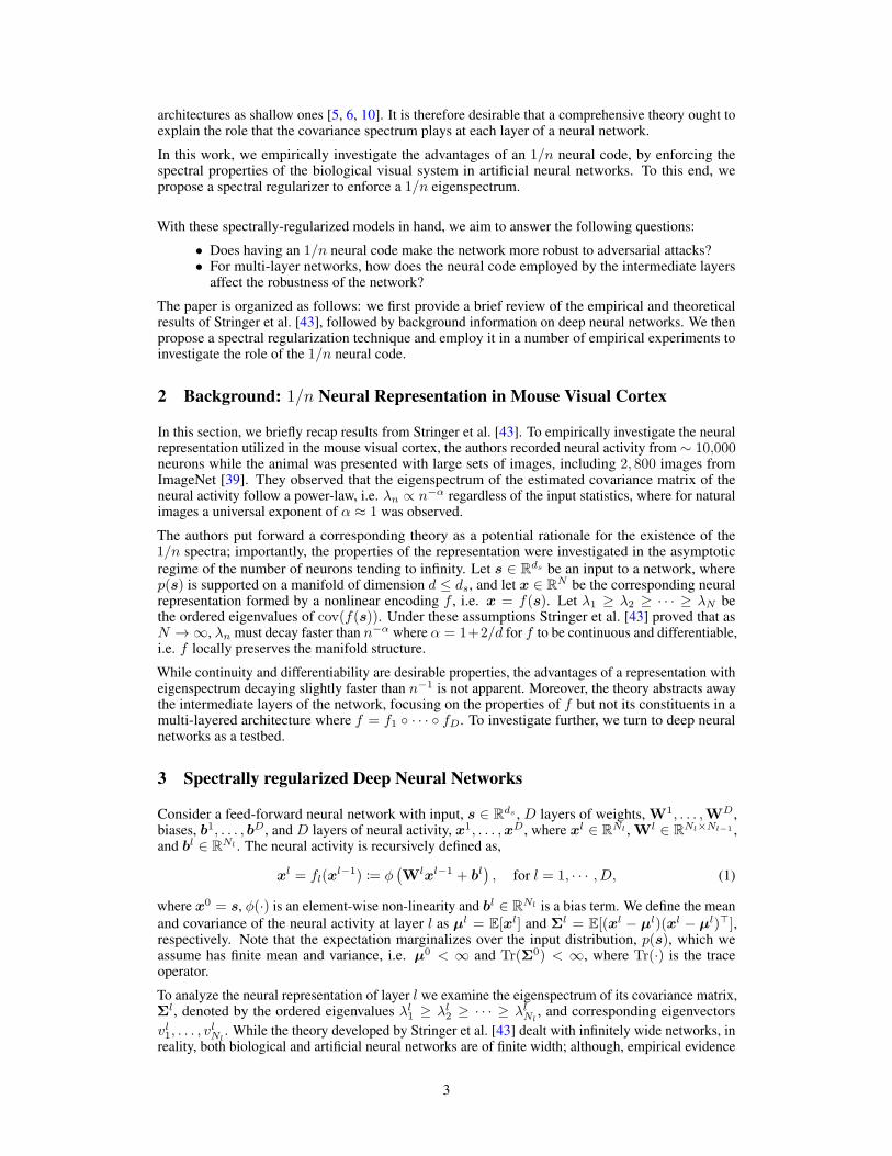
Figure 1: Studying the benefits of the spectrum of neural code for adversarial robustness. Theneural code of the biological brain shows 1/n power-law spectrum and also robust. Meaningfulmanifolds in the input space can gain nonlinear features or lose their structure depending on thepower-law exponent ↵. Using artificial neural networks and statistical whitening, we investigate howthe “dimensionality”, controlled by ↵, of the neural code impacts its robustness.

In this work, we use adversarial robustness to probe ideas regarding the ‘dimensionality’ of neuralrepresentations. The neuroscience community has advanced several normative theories, whichinclude optimal coding [4], sparse coding [17, 35], as well a host of experimental data and statisticalmodels [8, 18, 20, 22, 42] – resulting in, often conflicting, arguments in support of the prevalenceof both low-dimensional and high-dimensional neural codes. By comparison, the machine learningcommunity inspected the properties of hidden unit representations through the lens of statisticallearning theory [15, 34, 47], information theory [40, 46], and mean-field and kernel methods [12,27, 36]. The last two, by considering the limiting behavior as the number of neurons per layer goesto infinity, have been particularly successful, allowing analytical treatment of optimization, andgeneralization [2, 6, 7, 27].

Paralleling this development, a recent study recorded from a large number of mouse early visualarea (V1) neurons [43]. The statistical analysis of the data leveraged kernel methods, much likethe mean-field methods mentioned above, and has revealed that the covariance between neurons(marginalized over input) had a spectrum that decayed as a 1/n power-law regardless of the inputimage statistics. To provide a potential rationale for the representation to be poised between lowand high dimensionality, the authors developed a corresponding theory that relates the spectrum ofthe neural repertoire to the continuity and mean-square differentiability of a manifold in the inputspace [43]. Even with this proposed theory, the mechanistic role of the 1/n neural code is not known,but Stringer et al. [43] conjectured that it strikes a balance between expressivity and robustness.Moreover, the proposed theory only investigated the relationship between the input and output ofthe neural network; as many neural networks involve multiple layers, it is not clear how the neuralcode used by the intermediate layers affects the network as a whole. Similarly existing literaturethat relates the spectra of kernels to their out-of-sample generalization implicitly treats multi-layer

2

architectures as shallow ones [5, 6, 10]. It is therefore desirable that a comprehensive theory ought toexplain the role that the covariance spectrum plays at each layer of a neural network.

In this work, we empirically investigate the advantages of an 1/n neural code, by enforcing thespectral properties of the biological visual system in artificial neural networks. To this end, wepropose a spectral regularizer to enforce a 1/n eigenspectrum.

With these spectrally-regularized models in hand, we aim to answer the following questions:

• Does having an 1/n neural code make the network more robust to adversarial attacks?• For multi-layer networks, how does the neural code employed by the intermediate layers

affect the robustness of the network?

The paper is organized as follows: we first provide a brief review of the empirical and theoreticalresults of Stringer et al. [43], followed by background information on deep neural networks. We thenpropose a spectral regularization technique and employ it in a number of empirical experiments toinvestigate the role of the 1/n neural code.

2 Background: 1/n Neural Representation in Mouse Visual Cortex

In this section, we briefly recap results from Stringer et al. [43]. To empirically investigate the neuralrepresentation utilized in the mouse visual cortex, the authors recorded neural activity from ⇠ 10,000neurons while the animal was presented with large sets of images, including 2, 800 images fromImageNet [39]. They observed that the eigenspectrum of the estimated covariance matrix of theneural activity follow a power-law, i.e. �n / n�↵ regardless of the input statistics, where for naturalimages a universal exponent of ↵ ⇡ 1 was observed.

The authors put forward a corresponding theory as a potential rationale for the existence of the1/n spectra; importantly, the properties of the representation were investigated in the asymptotic

regime of the number of neurons tending to infinity. Let s 2 Rds be an input to a network, where

p(s) is supported on a manifold of dimension d ds, and let x 2 RN be the corresponding neural

representation formed by a nonlinear encoding f , i.e. x = f(s). Let �1 � �2 � · · · � �N bethe ordered eigenvalues of cov(f(s)). Under these assumptions Stringer et al. [43] proved that asN !1, �n must decay faster than n�↵ where ↵ = 1+2/d for f to be continuous and differentiable,i.e. f locally preserves the manifold structure.

While continuity and differentiability are desirable properties, the advantages of a representation witheigenspectrum decaying slightly faster than n�1 is not apparent. Moreover, the theory abstracts awaythe intermediate layers of the network, focusing on the properties of f but not its constituents in amulti-layered architecture where f = f1 � · · · � fD. To investigate further, we turn to deep neuralnetworks as a testbed.

3 Spectrally regularized Deep Neural Networks

Consider a feed-forward neural network with input, s 2 Rds , D layers of weights, W1, . . . ,WD,

biases, b1, . . . , bD, and D layers of neural activity, x1, . . . ,xD, where xl 2 RNl , Wl 2 R

Nl⇥Nl−1 ,and bl 2 R

Nl . The neural activity is recursively defined as,

xl = fl(xl�1) := �

�

Wlxl�1 + bl

�

, for l = 1, · · · , D, (1)

where x0 = s, �(·) is an element-wise non-linearity and bl 2 RNl is a bias term. We define the mean

and covariance of the neural activity at layer l as µl = E[xl] and Σl = E[(xl � µl)(xl � µl)>],

respectively. Note that the expectation marginalizes over the input distribution, p(s), which weassume has finite mean and variance, i.e. µ0 < 1 and Tr(Σ0) < 1, where Tr(·) is the traceoperator.

To analyze the neural representation of layer l we examine the eigenspectrum of its covariance matrix,Σ

l, denoted by the ordered eigenvalues �l1� �l

2� · · · � �l

Nl, and corresponding eigenvectors

vl1, . . . , vlNl

. While the theory developed by Stringer et al. [43] dealt with infinitely wide networks, inreality, both biological and artificial neural networks are of finite width; although, empirical evidence

3

has shown that the consequences of infinitely wide networks are still felt by finite-width networksthat are sufficiently wide [27, 36].

3.1 Spectral regularizer

In general, the distribution of eigenvalues of a deep neural network (DNN) is intractable and apriori there is no reason to believe it should follow a power-law — indeed, it will be determinedby architectural choices, such as initial weight distribution and non-linearity, but also by the entiretrajectory in parameter space traversed during optimization [27, 36]. A simple way to enforce apower-law decay without changing its architecture is to use the finite-dimensional embedding anddirectly regularize the eigenspectrum of the neural representation used at layer l. To this end weintroduce the following regularizer:

Rl(�l1, . . . ,�l

Nl) =

�

Nl

NlX

n�⌧

⇣

(�ln/�

ln � 1)2 +max(0,�l

n/�ln � 1)

⌘

, (2)

where �ln is a target sequence that follows a n�↵l power-law, ⌧ is a cut-off that dictates which

eigenvalues should be regularized and � is a hyperparameter that controls the strength of the reg-ularizer. To construct �l

n, we create a sequence of the form �ln = n�↵l where is chosen such

that �l⌧= �l

⌧. Since �l

⌧= �l

⌧, the ratio �l

n/�ln for n � ⌧ serves as a proxy measure to compare

the rates of decay between the eigenvalues, �ln, and the target sequence, �l

n. Leveraging this ratio,

(�ln/�

ln � 1)2 penalizes the network for using neural representations that stray away from �l

n; wenote that this term equally penalizes a ratio that is greater than or less than 1. Noting that having aslowly decaying spectrum, �l

n/�ln > 1, leads to highly undesirable properties (viz. discontinuity and

unbounded gradients in the infinite-dimensional case), max(0,�ln/�

ln � 1) is used to further penalize

the network for having a spectrum that decays too slowly.

3.2 Training scheme

Naive use of (2) as a regularizer faces practical difficulty as it requires estimating the eigenvaluesof the covariance matrix for each layer l of each mini-batch, which has a computational complexityof O(N3

l ). Obtaining a reasonable estimate of �jn also requires a batch size at least as large as the

widest layer in the network [11]. While the second issue is unavoidable, we propose a work aroundfor the first one.

Performing an eigenvalue decomposition of Σl gives

Σl = VlΛ

lV

>l , (3)

where Vl is an orthonormal matrix of eigenvectors and Λl is a diagonal matrix with the eigenvalues

of Σl on the diagonal. Using Vl we can diagonalize Σl to obtain

V>l Σ

lVl = Λ

l. (4)

It’s evident from (4) that given the eigenvectors, we could easily obtain the eigenvalues. Thus, wepropose the following approach: at the beginning of each epoch an eigenvalue decomposition isperformed on the full training set and the eigenvectors, Vl for l = 1, · · · , D, are stored. Next, foreach mini-batch we construct Σl and compute

V>l Σ

lVl = Λ̂

l, (5)

and the diagonal elements of Λ̂l are taken as an approximation for the true eigenvalues and used toevaluate (2). This approach is correct in the limit of vanishingly small learning rates [45].

When using the regularizer for training, the approximate eigenvectors are fixed and gradients are notback-propagated through them. Similar to batch normalization [26], the gradients are back-propagatedthrough the construction of the empirical covariance matrix, Σl.

4 Experiments

To empirically investigate the benefits of a power-law neural representation and of the proposedregularization scheme, we train a variety of models on MNIST [30]. While MNIST is considered

4

a toy dataset for most computer vision tasks, it is still a good test-bed for the design of adversarialdefenses [41]. Moreover, running experiments on MNIST has many advantages: 1) its simplicitymakes it easy to design and train highly-expressive DNNs without relying on techniques like dropoutor batch-norm; and 2) the models were able to be trained using a small learning rate, ensuring theefficacy of the training procedure detailed in section 3.2. This allows for the isolation of the effects ofa 1/n neural representation, which may not have been possible if we used a dataset like CIFAR-10.

Recall that the application of Stringer et al. [43]’s theory requires an estimate of the manifolddimension, d, which is not known for MNIST. However, we make the simplifying assumption that itis sufficiently large such that 1 + 2/d ⇡ 1 holds. For this reason we set ↵l = 1 for all experiments.Based on the empirical observation of Stringer et al. [43], we set ⌧ = 10 as they observed thatthe neural activity of the mouse visual cortex followed a power-law approximately after the tentheigenvalue. For all experiments three different values of � were tested, � 2 {1, 2, 5}, and the resultsof the best one are shown in the main text (results for all values of � are deferred to the appendix).The networks were optimized using Adam [29], where a learning rate of 10�4 was chosen to ensurethe stability of the proposed training scheme. For each network, the batch size is chosen to be 1.5times larger than the widest layer in the network. All results shown are based on 3 experiments withdifferent random seeds2.

The robustness of the models are evaluated against two popular forms of adversarial attacks:

• Fast gradient sign method (FGSM): Given an input image, sn, and corresponding label, yn,FGSM [23] produces an adversarial image, s̃n, by

s̃n = sn + ✏ sign(rsnL(f(sn; ✓), yn)), (6)

where L(·, ·) is the loss function and sign(·) is the sign function.

• Projected gradient descent (PGD): Given an input image, sn, and corresponding label, yn,PGD [32] produces an adversarial image, s̃n, by solving the following optimization problem

argmaxδ

L(f(sn + δ;θ), yn),

such that kδk1 ✏.(7)

To approximately solve (7), we use 40 steps of projected gradient descent

δ Projkδk∞✏(δ + ⌘rδL(f(sn + δ;θ), yn)) , (8)

where we set ⌘ = 0.01 and Projkδk∞✏(·) is the projection operator.

The models are also evaluated on white noise corrupted images though we defer these results to theappendix.

To attempt to understand the features utilized by the neural representations, we visualize

Jn(xj) =@�D

n

@xj

. (9)

where �Dn is the nth eigenvalue of ΣD. To compute (9), the full data set is passed through the network

to obtain ΣD. The eigenvalues are then computed and gradients are back-propagated through the

operation to obtain (9).

4.1 Shallow Neural Networks

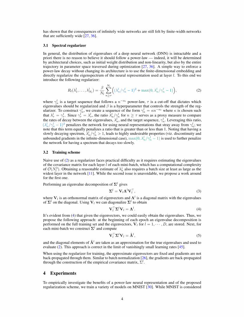
To isolate the benefits of a 1/n neural representation, we begin by applying the proposed spectralregularizer on a sigmoidal neural network with one hidden layer of N1 = 2,000 neurons with batchnorm [26] (denoted by SpecReg) and examine its robustness to adversarial attacks. As a baseline, wecompare it against a vanilla (unregularized) network.

Figure 2A, demonstrates the efficacy of the proposed training scheme as the spectra of the regularizednetwork follows 1/n pretty closely. Figures 2B and C demonstrate that a spectrally regularizednetwork is significantly more robust than it’s vanilla counterpart against both FGSM and PGD attacks.

2Code is available at https://github.com/josuenassar/power_law

5

While the results are nowhere near SOTA, we emphasize that this robustness was gained withouttraining on a single adversarial image, unlike other approaches. The spectrally regularized networkhas a much higher effective dimension (Fig. 2A), and it learns a more relevant set of features asindicated by the sensitivity maps (Fig. 2D). We note that while the use of batch norm helped toincrease the effectiveness of the spectral regularizer, it did not affect on the robustness of the vanillanetwork. In the interest of space, the results for the networks without batch norm are in the appendix.

B CA

More robust!

Vanilla

SpecReg

D n=1input 2 5 10 20 50 100 500 1000Jn

Figure 2: A 1/n neural representation leads to more robust networks. A) Eigenspectrum of aregularly trained network, Vanilla, and a spectrally regularized network, SpecReg. The shaded greyarea are the eigenvalues that are not regularized. Star indicates the dimension at which the cumulativevariance exceeds 90%. B & C) Comparison of adversarial robustness between vanilla and spectrallyregularized networks where the shaded region is ± 1 standard deviation computed over 3 randomseeds. D) The sensitivity of �n with respect to the input image.

4.2 Deep Neural Networks

Inspired by the results in the previous section, we turn our attention to deep neural networks.Specifically, we experiment on a multi-layer perceptron (MLP) with three hidden layers whereN1 = N2 = N3 = 1,000 and on a convolutional neural network (CNN) with three hidden layers:a convolutional layer with 16 output channels with a kernel size of (3, 3), followed by anotherconvolutional layer with 32 output channels with a kernel of size (3, 3) and a fully-connected layer ofwidth 1,000 neurons, where max-pooling is applied after each convolutional layer. To regularize theneural representation utilized by the convolutional layers, the output of all the channels is flattenedtogether and the spectrum of their covariance matrix is regularized. We note that no other form ofregularization is used to train these networks i.e. batch norm, dropout, weight decay, etc.

We demonstrate empirically the importance of intermediate layers in a deep neural network, asnetworks with "bad" intermediate representations are shown to be extremely brittle.

4.2.1 The Importance of Intermediate Layers in Deep Neural Networks

Theoretical insights from Stringer et al. [43] as well as other works [6, 27] do not prescribe how thespectrum of intermediate layers should behave for a “good” neural representation. Moreover, it is notclear how the neural representation employed by the intermediate layers will affect the robustnessof the overall network. The theory of Stringer et al. [43] suggests that the intermediate layers of thenetwork do not matter as long as the neural representation of the last hidden layer is 1/n.

To investigate the importance of the intermediate layers, we “break” the neural representation of thesecond hidden layer by whitening its neural activity

x̃2 = R�1

2(x2 � µ2) (10)

6

n=1input 2 5 10 20 50 100 500 1000whitening

SpecReg

Jacobian

A

B

C

D

E

F

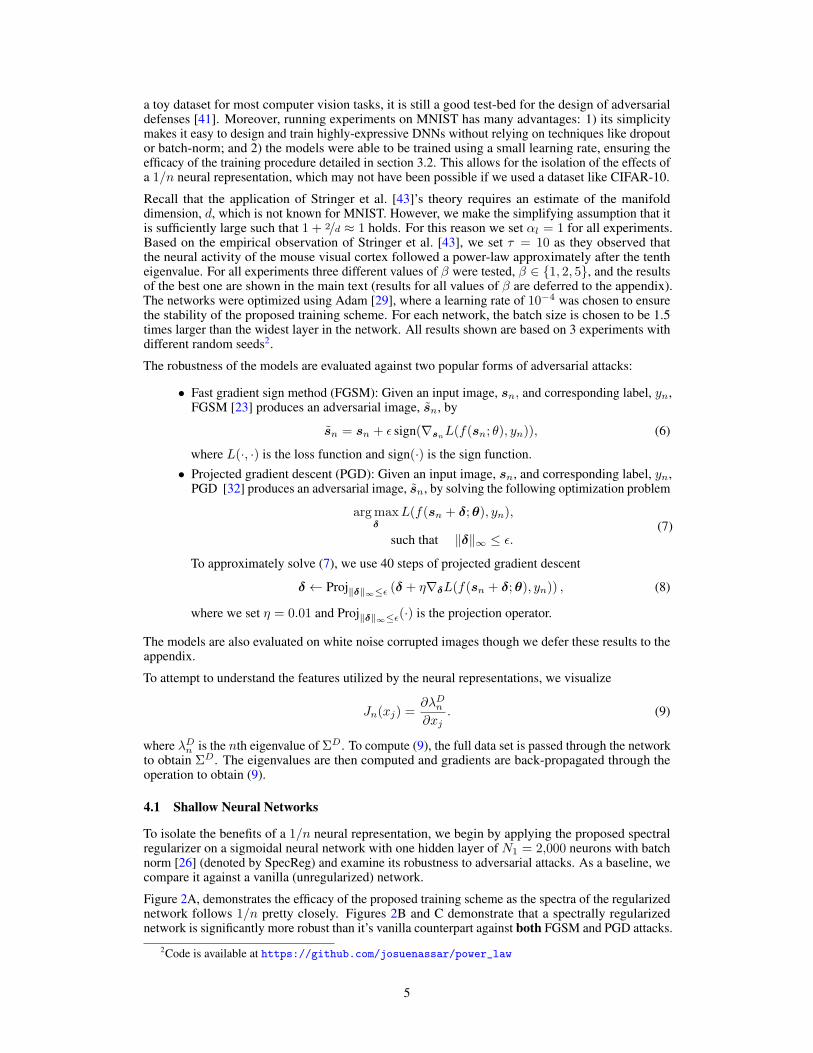
Jn

Figure 3: Sensitivity maps for 3-layer multi-layer perceptrons. Each row corresponds to a differentexperiment: (A) MLP with whitening layer, (B) SpecReg only on the last layer after whitening,(C) SpecReg only on the last layer, (D) Vanilla MLP, (E) SpecReg on every layer, (F) Jacobianregularization. Each sensitivity image corresponds to the n-th eigenvalue on the last hidden layer.

where R2 is the Cholesky decomposition of Σ2, leading to a flat spectrum which is the worst casescenario under the asymptotic theory in Stringer et al. [43]. To compute (10), the sample mean, µ̂2,

and covariance, Σ̂2, are computed for each mini-batch. Training with the whitening operation ishandled similarly to batch norm [26], where gradients are back-propagated through the sample mean,covariance and Cholesky decomposition.

MLP CNN

Vanilla

Vanilla-Wh

SpecReg

SpecReg-Wh

A B C D

Figure 4: Spectral regularization does not rescue robustness lost by whitening the intermediaterepresentation. (A,B) For MLP, adversarial robustness for FGSM and PGD indicates a more fragilecode resulting from whitening. Spectral regularization of the last hidden layer does not improverobustness. (C,D) For CNNs, spectral regularization of the last layer enhances robustness, but forMLPs it does not. Same conventions as Fig. 2B,C and Fig. 3.

When the intermediate layer is whitened, the resulting sensitivity features lose structure (Fig. 3Acompared to Fig. 3D). This network is less robust to adversarial attacks (Fig. 4A,B dashed black)consistent with the structureless sensitivity map.

We added spectral regularization to the last hidden layer in hopes of salvaging the network (seeSec. 3.2 for details). Although the resulting spectrum of the last layer shows a 1/n tail (Fig. A10), therobustness is not improved (Fig. 4A,B). Applying the asymptotic theory to the whitened output, the

7

neural representation is “bad” and the manifold becomes non-differentiable. Spectral regularizationof the last hidden layer cannot further fix this broken representation even in a finite-sized network(Fig. 3B).

Interestingly, for the MLP, regularizing only the last hidden layer (without whitening) improved thesensitivity map (Fig. 3C) but had no effect on the robustness of the network (Fig. 4A,B), suggestingthat a 1/n neural representation at the last hidden layer is not sufficient. In contrast, regularizing thelast hidden layer of the CNN does increase the robustness of the network (Fig. 4C,D).

4.3 Regularizing all layers of the network increases adversarial robustness

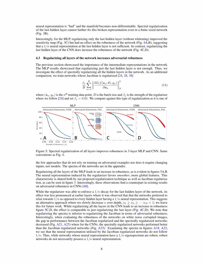
The previous section showcased the importance of the intermediate representations in the network.The MLP results showcased that regularizing just the last hidden layer is not enough. Thus, weinvestigate the effect of spectrally regularizing all the hidden layers in the network. As an additionalcomparison, we train networks whose Jacobian is regularized [24, 28, 38]

�j

B

BX

n=1

�

�

�

�

@L(f(sn; ✓), yn)

@sn

�

�

�

�

2

F

(11)

where (sn, yn) is the nth training data point, B is the batch size and �j is the strength of the regularizerwhere we follow [24] and set �j = 0.01. We compare against this type of regularization as it is one of

A B C D

Vanilla

Vanilla

Jacobian

SpecRegJacobian

SpecReg

MLP CNN

Figure 5: Spectral regularization of all layers improves robustness in 3-layer MLP and CNN. Sameconventions as Fig. 4.

the few approaches that do not rely on training on adversarial examples nor does it require changinginputs, nor models. The spectra of the networks are in the appendix.

Regularizing all the layers of the MLP leads to an increase in robustness, as is evident in figures 5A,B.The neural representation induced by the regularizer favors smoother, more global features. Thischaracteristic is shared both by our proposed regularization technique as well as Jacobian regulariza-tion, as can be seen in figure 3. Interestingly, these observations find a counterpart in existing resultson adversarial robustness in CNNs [48].

While the regularizer was able to enforce a 1/n decay for the last hidden layer of the network, itseffect was less pronounced at earlier layers where it was observed that that the networks preferred torelax towards 1/n as opposed to every hidden layer having a 1/n neural representation. This suggestsan alternative approach where we slowly decrease ↵ over depth, ↵1 � ↵2 � · · ·↵D = 1; we leavethis for future work. While regularizing all the layers in the CNN leads to an increase in robustnessfigure 5C,D, the effect is comparable to just regularizing the last layer (Fig. 4C,D). We note thatregularizing the spectra is inferior to regularizing the Jacobian in terms of adversarial robustness.Interestingly, when evaluating the robustness of the networks on white noise corrupted images,the gap in performance between the Jacobian regularized and the spectrally regularized networksdecreased (Fig. A21, A25) where for the CNNs, the spectrally regularized networks performed betterthan the Jacobian regularized networks (Fig. A25). Examining the spectra in figures A18, A22,we see that the neural representation utilized by the Jacobian regularized networks do not follow1/n. Thus, while networks whose neural representation have a 1/n eigenspectrum are robust, robustnetworks do not necessarily possess a 1/n neural representation.

8

5 Discussion

In this study, we trained artificial neural networks using a novel spectral regularizer to furtherunderstand the benefits and intricacies of a 1/n spectra in neural representations. We note that ourcurrent implementation of the spectral regularization is not intended to be used in general but rather astraightforward embodiment of the study objective. As the result suggests, a general encouragementof 1/n-like spectrum could be beneficial in wide neural networks, and special architectures could bedesigned to more easily achieve this goal. The results have also helped to elucidate the importanceof intermediate layers in DNNs and may offer a potential explanation for why batch normalizationreduces the robustness of DNNs [19]. Furthermore, the results contribute to a growing body ofliterature that analyzes the generalization of artificial neural networks from the perspective of kernelmachines (viz [6, 27]). As mentioned before, the focus in those works is on the input-output mapping,which does away with the intricate structure of representations at intermediate layers. In this work,we take an empirical approach and probe how the neural code for different hidden layers contributesto overall robustness.

From a neuroscientific perspective, it is interesting to conjecture whether a similar power-law codewith a similar exponent is a hallmark of canonical cortical computation, or whether it reflects theunique specialization of lower visual areas. Existing results in theoretical neuroscience point to the factneural code dimensionality in visual processing is likely to be either transiently increasing and thendecreasing as stimuli are propagated to downstream neurons, or monotonically decreasing [3, 9, 13].Resolving the question of the ubiquity of power-law-like codes with particular exponents can thereforebe simultaneously addressed in-vivo and in-silico, with synthetic experiments probing differentexponents at higher layers in an artificial neural network. Moreover, this curiously relates to theobserved, but commonplace spectrum flattening for random deep neural networks [36], and questionsabout its effect on information propagation. We leave these questions for future study.

Broader Impact

Adversarial attacks pose threats to the safe deployment of AI systems– both safety from maliciousattacks but also robustness that would be expected in intelligent devices such as self-driving cars [37]but also facial recognition systems. Our neuroscience-inspired approach, unlike widely use adversarialattack defenses, does not require generation of adversarial input samples, therefore it potentiallyavoids the pitfalls of unrepresentative datasets. Furthermore, our study shows possibilities for theimprovement of artificial systems with insights gained from biological systems which are naturallyrobust. Conversely it also provides a deeper, mechanistic understanding of experimental data fromthe field of neuroscience, thereby advancing both fields at the same time.

Acknowledgments and Disclosure of Funding

This work is supported by the generous support of Stony Brook Foundation’s Discovery Award, NSFCAREER IIS-1845836, NSF IIS-1734910, NIH/NIBIB EB026946, and NIH/NINDS UF1NS115779.JN was supported by the STRIDE fellowship at Stony Brook University. SYC was supported by theNSF NeuroNex Award DBI-1707398 and the Gatsby Charitable Foundation. KDH was supported byWellcome Trust grants 108726 and 205093. JN thanks Kendall Lowrey, Benjamin Evans and YousefEl-Laham for insightful discussions and feedback. JN also thanks the Methods in ComputationalNeuroscience Course at the Marine Biological Laboratory in Woods Hole, MA for bringing us alltogether and for the friends, teaching assistants, and faculty who provided insightful discussions,support and feedback.

References

[1] D. H. Ackley, G. E. Hinton, and T. J. Sejnowski. A Learning Algorithm for Boltzmann Machines.Cognitive Science, 9(1):147–169, 1985.

[2] Z. Allen-Zhu, Y. Li, and Y. Liang. Learning and Generalization in Overparameterized NeuralNetworks, Going Beyond Two Layers. arXiv:1811.04918 [cs, math, stat], May 2019.

9

[3] A. Ansuini, A. Laio, J. H. Macke, and D. Zoccolan. Intrinsic dimension of data representationsin deep neural networks. In Advances in Neural Information Processing Systems, pages 6111–6122, 2019.

[4] H. B. Barlow. Possible Principles Underlying the Transformations of Sensory Messages. TheMIT Press, 1953. ISBN 978-0-262-31421-3.

[5] P. L. Bartlett, O. Bousquet, and S. Mendelson. Local Rademacher complexities. The Annals ofStatistics, 33(4):1497–1537, Aug. 2005. ISSN 0090-5364, 2168-8966.

[6] B. Bordelon, A. Canatar, and C. Pehlevan. Spectrum Dependent Learning Curves in KernelRegression and Wide Neural Networks. arXiv:2002.02561 [cs, stat], Feb. 2020.

[7] L. Chizat, E. Oyallon, and F. Bach. On Lazy Training in Differentiable Programming. InH. Wallach, H. Larochelle, A. Beygelzimer, F. Alché-Buc, E. Fox, and R. Garnett, editors,Advances in Neural Information Processing Systems 32, pages 2937–2947. Curran Associates,Inc., 2019.

[8] M. M. Churchland, J. P. Cunningham, M. T. Kaufman, J. D. Foster, P. Nuyujukian, S. I. Ryu,and K. V. Shenoy. Neural population dynamics during reaching. Nature, 487(7405):51–56, July2012. ISSN 0028-0836, 1476-4687.

[9] U. Cohen, S. Chung, D. D. Lee, and H. Sompolinsky. Separability and geometry of objectmanifolds in deep neural networks. Nature communications, 11(1):1–13, 2020.

[10] C. Cortes, M. Kloft, and M. Mohri. Learning kernels using local rademacher complexity. InC. J. C. Burges, L. Bottou, M. Welling, Z. Ghahramani, and K. Q. Weinberger, editors, Advancesin Neural Information Processing Systems 26, pages 2760–2768. Curran Associates, Inc., 2013.

[11] R. Couillet and M. Debbah. Random matrix methods for wireless communications. CambridgeUniversity Press, 2011.

[12] A. Daniely, R. Frostig, and Y. Singer. Toward Deeper Understanding of Neural Networks: ThePower of Initialization and a Dual View on Expressivity. In D. D. Lee, M. Sugiyama, U. vonLuxburg, I. Guyon, and R. Garnett, editors, Advances in Neural Information Processing Systems29: Annual Conference on Neural Information Processing Systems 2016, December 5-10, 2016,Barcelona, Spain, pages 2253–2261, 2016.

[13] J. J. DiCarlo and D. D. Cox. Untangling invariant object recognition. Trends in cognitivesciences, 11(8):333–341, 2007.

[14] E. Dohmatob. Generalized No Free Lunch Theorem for Adversarial Robustness. In InternationalConference on Machine Learning, pages 1646–1654, May 2019.

[15] G. K. Dziugaite and D. M. Roy. Computing Nonvacuous Generalization Bounds for Deep(Stochastic) Neural Networks with Many More Parameters than Training Data. In G. Elidan,K. Kersting, and A. T. Ihler, editors, Proceedings of the Thirty-Third Conference on Uncertaintyin Artificial Intelligence, UAI 2017, Sydney, Australia, August 11-15, 2017. AUAI Press, 2017.

[16] K. Fukushima. Neocognitron: A self-organizing neural network model for a mechanism ofpattern recognition unaffected by shift in position. Biological Cybernetics, 36(4):193–202, Apr.1980. ISSN 0340-1200, 1432-0770.

[17] S. Fusi, E. K. Miller, and M. Rigotti. Why neurons mix: high dimensionality for highercognition. Current opinion in neurobiology, 37:66–74, Apr. 2016. ISSN 0959-4388, 1873-6882.

[18] J. A. Gallego, M. G. Perich, S. N. Naufel, C. Ethier, S. A. Solla, and L. E. Miller. Corticalpopulation activity within a preserved neural manifold underlies multiple motor behaviors.Nature Communications, 9(1):1–13, Oct. 2018. ISSN 2041-1723.

[19] A. Galloway, A. Golubeva, T. Tanay, M. Moussa, and G. W. Taylor. Batch normalization is acause of adversarial vulnerability. arXiv preprint arXiv:1905.02161, 2019.

[20] P. Gao and S. Ganguli. On simplicity and complexity in the brave new world of Large-Scaleneuroscience. Current opinion in neurobiology, 32:148–155, Mar. 2015. ISSN 0959-4388.

10

[21] R. Geirhos, P. Rubisch, C. Michaelis, M. Bethge, F. A. Wichmann, and W. Brendel. Imagenet-trained CNNs are biased towards texture; increasing shape bias improves accuracy and robust-ness. In International Conference on Learning Representations, 2019.

[22] M. D. Golub, P. T. Sadtler, E. R. Oby, K. M. Quick, S. I. Ryu, E. C. Tyler-Kabara, A. P. Batista,S. M. Chase, and B. M. Yu. Learning by neural reassociation. Nature neuroscience, 21(4):607–616, Apr. 2018. ISSN 1097-6256, 1546-1726.

[23] I. J. Goodfellow, J. Shlens, and C. Szegedy. Explaining and harnessing adversarial examples.arXiv preprint arXiv:1412.6572, 2014.

[24] J. Hoffman, D. A. Roberts, and S. Yaida. Robust learning with jacobian regularization. arXivpreprint arXiv:1908.02729, 2019.

[25] A. Ilyas, S. Santurkar, D. Tsipras, L. Engstrom, B. Tran, and A. Madry. Adversarial examplesare not bugs, they are features. arXiv preprint arXiv:1905.02175, 2019.

[26] S. Ioffe and C. Szegedy. Batch normalization: Accelerating deep network training by reducinginternal covariate shift. arXiv preprint arXiv:1502.03167, 2015.

[27] A. Jacot, F. Gabriel, and C. Hongler. Neural tangent kernel: Convergence and generalizationin neural networks. In Advances in neural information processing systems, pages 8571–8580,2018.

[28] D. Jakubovitz and R. Giryes. Improving DNN Robustness to Adversarial Attacks using JacobianRegularization. In Proceedings of the European Conference on Computer Vision (ECCV), pages514–529, 2018.

[29] D. P. Kingma and J. Ba. Adam: A method for stochastic optimization. arXiv preprintarXiv:1412.6980, 2014.

[30] Y. LeCun, L. Bottou, Y. Bengio, P. Haffner, et al. Gradient-based learning applied to documentrecognition. Proceedings of the IEEE, 86(11):2278–2324, 1998.

[31] Y. LeCun, Y. Bengio, and G. Hinton. Deep learning. Nature, 521(7553):436–444, May 2015.ISSN 1476-4687.

[32] A. Madry, A. Makelov, L. Schmidt, D. Tsipras, and A. Vladu. Towards deep learning modelsresistant to adversarial attacks. In International Conference on Learning Representations, 2018.

[33] W. S. McCulloch and W. Pitts. A logical calculus of the ideas immanent in nervous activity.The bulletin of mathematical biophysics, 5(4):115–133, Dec. 1943. ISSN 1522-9602.

[34] B. Neyshabur, S. Bhojanapalli, D. Mcallester, and N. Srebro. Exploring Generalization in DeepLearning. In I. Guyon, U. V. Luxburg, S. Bengio, H. Wallach, R. Fergus, S. Vishwanathan, andR. Garnett, editors, Advances in Neural Information Processing Systems 30, pages 5947–5956.Curran Associates, Inc., 2017.

[35] B. A. Olshausen and D. J. Field. Emergence of simple-cell receptive field properties by learninga sparse code for natural images. Nature, 381(6583):607–609, June 1996. ISSN 0028-0836.

[36] B. Poole, S. Lahiri, M. Raghu, J. Sohl-Dickstein, and S. Ganguli. Exponential expressivity indeep neural networks through transient chaos. In Advances in neural information processingsystems, pages 3360–3368, 2016.

[37] A. Ranjan, J. Janai, A. Geiger, and M. J. Black. Attacking Optical Flow. In 2019 IEEE/CVFInternational Conference on Computer Vision, ICCV 2019, Seoul, Korea (South), October 27 -November 2, 2019, pages 2404–2413. IEEE, 2019.

[38] A. S. Ross. Improving the Adversarial Robustness and Interpretability of Deep Neural Networksby Regularizing Their Input Gradients. pages 1660–1669, 2018.

[39] O. Russakovsky, J. Deng, H. Su, J. Krause, S. Satheesh, S. Ma, Z. Huang, A. Karpathy,A. Khosla, M. Bernstein, et al. Imagenet large scale visual recognition challenge. Internationaljournal of computer vision, 115(3):211–252, 2015.

11

[40] A. M. Saxe, Y. Bansal, J. Dapello, M. Advani, A. Kolchinsky, B. D. Tracey, and D. D. Cox.On the Information Bottleneck Theory of Deep Learning. In 6th International Conferenceon Learning Representations, ICLR 2018, Vancouver, BC, Canada, April 30 - May 3, 2018,Conference Track Proceedings. OpenReview.net, 2018.

[41] L. Schott, J. Rauber, M. Bethge, and W. Brendel. Towards the first adversarially robust neuralnetwork model on MNIST. In International Conference on Learning Representations, 2019.

[42] H. Sohn, D. Narain, N. Meirhaeghe, and M. Jazayeri. Bayesian computation through corticallatent dynamics. Neuron, 103(5):934–947.e5, Sept. 2019. ISSN 0896-6273, 1097-4199.

[43] C. Stringer, M. Pachitariu, N. Steinmetz, M. Carandini, and K. D. Harris. High-dimensionalgeometry of population responses in visual cortex. Nature, page 1, 2019.

[44] C. Szegedy, W. Zaremba, I. Sutskever, J. Bruna, D. Erhan, I. Goodfellow, and R. Fergus.Intriguing properties of neural networks. arXiv preprint arXiv:1312.6199, 2013.

[45] T. Tao. Topics in random matrix theory. Graduate Studies in Mathematics, 132, 2011.

[46] N. Tishby and N. Zaslavsky. Deep learning and the information bottleneck principle. In 2015IEEE Information Theory Workshop, ITW 2015, Jerusalem, Israel, April 26 - May 1, 2015,pages 1–5. IEEE, 2015.

[47] V. N. Vapnik. The Nature of Statistical Learning Theory. Springer, 1st ed. 1995. corr. 2ndprinting edition, Dec. 1998. ISBN 9780387945590.

[48] H. Wang, X. Wu, P. Yin, and E. P. Xing. High Frequency Component Helps Explain theGeneralization of Convolutional Neural Networks. arXiv:1905.13545 [cs], May 2019.

12