Neural Representation Learning in Linguistic Structured ...

September 27, 2016DRAFT

Neural Representation Learningin Linguistic Structured Prediction

Lingpeng Kong

October 2016

School of Computer ScienceCarnegie Mellon University

Pittsburgh, PA 15213

Thesis Committee:Noah A. Smith (co-Chair), Carnegie Mellon University / University of Washington

Chris Dyer (co-Chair), Carnegie Mellon UniversityAlan W. Black, Carnegie Mellon University

Michael Collins, Columbia University

Submitted in partial fulfillment of the requirementsfor the degree of Doctor of Philosophy.

Copyright c© 2016 Lingpeng Kong



AbstractAdvances in neural network architectures and training algorithms have demon-

strated the effectiveness of representation learning in natural language processing.This thesis stresses the importance of computationally modeling the structure in lan-guage, even when learning representations.

We propose that explicit structure representations and learned distributed repre-sentations can be efficiently combined for improved performance over (i) traditionalapproaches to structure and (ii) uninformed neural networks that ignore all but sur-face sequential structure. We demonstrate on three distinct problems how assump-tions about structure can be integrated naturally into neural representation learnersfor NLP problems, without sacrificing computational efficiency.

First, we introduce an efficient model for inferring the phrase-structure trees us-ing given dependency syntax trees as constraints and propose to extend the model,making it more expressive through non-linear (neural) representation learning.

Second, we propose segmental recurrent neural networks (SRNNs) which de-fine, given an input sequence, a joint probability distribution over segmentations ofthe input and labelings of the segments and show that comparing to models that donot explicitly represent segments such as BIO tagging schemes and connectionisttemporal classification (CTC), SRNNs obtain substantially higher accuracies.

Third, we consider the problem of Combinatory Categorial Grammar (CCG) su-pertagging. We propose to model the compositionality both inside these tags andbetween these tags. This enables the model to handle an unbounded number of su-pertags where structurally naive models simply fail.

The techniques proposed in this thesis automatically learn structurally informedrepresentations of the inputs. These representations and components in the mod-els can be better integrated with other end-to-end deep learning systems within andbeyond NLP.


iv


Contents

1 Introduction 1

2 Transforming Dependencies into Phrase Structures 32.1 Parsing Dependencies . . . . . . . . . . . . . . . . . . . . . . . . . . . . . . . . 3

2.1.1 Parsing Algorithm . . . . . . . . . . . . . . . . . . . . . . . . . . . . . 32.1.2 Pruning . . . . . . . . . . . . . . . . . . . . . . . . . . . . . . . . . . . 52.1.3 Binarization and Unary Rules . . . . . . . . . . . . . . . . . . . . . . . 6

2.2 Structured Prediction . . . . . . . . . . . . . . . . . . . . . . . . . . . . . . . . 72.2.1 Features . . . . . . . . . . . . . . . . . . . . . . . . . . . . . . . . . . . 72.2.2 Training . . . . . . . . . . . . . . . . . . . . . . . . . . . . . . . . . . . 8

2.3 Methods . . . . . . . . . . . . . . . . . . . . . . . . . . . . . . . . . . . . . . . 82.4 Experiments . . . . . . . . . . . . . . . . . . . . . . . . . . . . . . . . . . . . . 92.5 Proposed Work . . . . . . . . . . . . . . . . . . . . . . . . . . . . . . . . . . . 11

3 Segmental Recurrent Neural Networks 133.1 Model . . . . . . . . . . . . . . . . . . . . . . . . . . . . . . . . . . . . . . . . 133.2 Inference with Dynamic Programming . . . . . . . . . . . . . . . . . . . . . . . 14

3.2.1 Computing Segment Embeddings . . . . . . . . . . . . . . . . . . . . . 153.2.2 Computing the most probable segmentation/labeling and Z(x) . . . . . . 163.2.3 Computing Z(x,y) . . . . . . . . . . . . . . . . . . . . . . . . . . . . . 16

3.3 Parameter Learning . . . . . . . . . . . . . . . . . . . . . . . . . . . . . . . . . 173.4 Further Speedup . . . . . . . . . . . . . . . . . . . . . . . . . . . . . . . . . . . 173.5 Experiments . . . . . . . . . . . . . . . . . . . . . . . . . . . . . . . . . . . . . 18

3.5.1 Online Handwriting Recognition . . . . . . . . . . . . . . . . . . . . . . 183.5.2 End-to-end Speech Recognition . . . . . . . . . . . . . . . . . . . . . . 20

3.6 Conclusion . . . . . . . . . . . . . . . . . . . . . . . . . . . . . . . . . . . . . 22

4 Modeling the Compositionality in CCG Supertagging 234.1 CCG and Supertagging . . . . . . . . . . . . . . . . . . . . . . . . . . . . . . . 234.2 Supertagging Transition System . . . . . . . . . . . . . . . . . . . . . . . . . . 23

4.2.1 CCG Parsing Transition System . . . . . . . . . . . . . . . . . . . . . . 264.3 Conclusion . . . . . . . . . . . . . . . . . . . . . . . . . . . . . . . . . . . . . 27

5 Conclusion 29

v


6 Timeline 31

Bibliography 33

vi


Chapter 1

Introduction

Computationally modeling the structure in language is crucial for two reasons. First, for thelarger goal of automated language understanding, linguists have found that language meaning isderived through composition. Structure in language tells what are the atoms (e.g., words in asentence) and how they fit together (e.g., syntactic or semantic parses) in composition. Second,from the perspective of machine learning, linguistic structures can be understood as a form ofinductive bias, which helps learning succeed with less or less ideal data (Mitchell, 1980). Formany tasks in NLP, only limited amounts of supervision is available. Therefore, getting theinductive bias right is particular important.

In recent years, neural models are state-of-the-art for many NLP tasks, including speechrecognition (Graves et al., 2013), dependency parsing (Andor et al., 2016) and machine trans-lation (Bahdanau et al., 2015). For many applications, the model architecture combines denserepresentations of words (Manning, 2016) and with sequential recurrent neural networks (Dyeret al., 2016). Thus, while they generally make use of information about what the words are(rather than operating on sequences of characters), they ignore syntactic and semantic structureand thus can be criticized as being structurally naive.

This thesis argues that explicit structure representations and learned distributed representa-tions can be efficiently combined for improved performance over (i) traditional approaches tostructure and (ii) uninformed neural networks that ignore all but surface sequential structure. Asan example, Dyer et al. (2015) yields better accuracy than Chen and Manning (2014) by replac-ing the word representation on the stack with composed representations derived from linguisticstructure.

In the first part of the thesis, first published as Kong et al. (2015b), we introduce an efficientmodel for inferring the phrase-structure trees using given dependency syntax trees as constraints.Dependency parsers are generally much faster, but less informative, since they do not produceconstituents, which are often required by downstream applications. The approach we proposecan be understood as a specially-trained coarse-to-fine decoding algorithm where the dependencyparser provides “coarse” structure and the second stage refines it. Our algorithm achieved simi-lar performance as state-of-the-art lexicalized phrase-structure parsers while doing it much moreefficiently. This is an example of a structure-to-structure mapping problem that does not quitefit into the currently available neural frameworks that focus on sequences. We will extend the

1


previous work, making such model more expressive through non-linear (neural) representationlearning, while still making use of the structural information available as input and producingwell-formed structural output. This will serve as an example of integrating structural and neuralmodels.

In the second part of this thesis, first published as (Kong et al., 2015a; Lu et al., 2016), wepropose segmental recurrent neural networks (SRNNs) which define, given an input sequence,a joint probability distribution over segmentations of the input and labelings of the segments.Traditional neural solutions to this problem, e.g., connectionist temporal classification (CTC)(Graves et al., 2006a), reduce the segmental sequence labeling problem to a sequence labelingproblem in the same spirit as BIO tagging. In our model, representations of the input segments(i.e., contiguous subsequences of the input) are computed by composing their constituent tokensusing bidirectional recurrent neural nets, and these segment embeddings are used to define com-patibility scores with output labels. Our model achieves competitive results in phone recognition,handwriting recognition, and joint word segmentation & POS tagging.

In the third part of the thesis, we consider the problem of Combinatory Categorial Grammar(CCG) supertagging (Steedman, 2000). CCG is widely used in semantic parsing, and parsingwith it is very fast, especially if there’s a good (probabilistic) tagger (Lewis and Steedman, 2014a;Lee et al., 2016). While the Penn Treebank (Marcus et al., 1993) has just 50 fixed POS tags, tag-ging the same corpus with CCG supertags uses over 400 lexical categories (i.e., supertags) and,in general, this number is unbounded since tags may be created productively. Current taggers(Lewis and Steedman, 2014a; Xu et al., 2015b; Lewis and Steedman, 2014b, inter alia) simplytreat these supertags as discrete categories. We propose to model the compositionality both insidethese tags and between these tags (even when not doing parsing, the compositionality betweenthe tags can be modeled as a sequence level loss inside the model). Previous works suggests thatexplicitly modeling the compositional aspect of supertags can lead to better accuracy (Srikumarand Manning, 2014) and less supervision (Garrette et al., 2015).

In this thesis, we stress the importance of explicitly representing structure in neural models.We demonstrate on three distinct problems how assumptions about structure can be integratednaturally into neural representation learners for NLP problems, without sacrificing computationalefficiency. We argue that, when comparing with structurally naive models, models that reasonabout the internal linguistic structure of the data demonstrate better generalization performance.

2


Chapter 2

Transforming Dependencies into PhraseStructures

Our prior work (Kong et al., 2015b) introduces an efficient model for inferring the phrase-structure trees using given dependency syntax trees as constraints. Because dependency parsersare generally much faster than phrase-structure parsers, we consider an alternate pipeline (Sec-tion 2.1): dependency parse first, then transform the dependency representation into a phrase-structure tree constrained to be consistent with the dependency parse. This idea was exploredby Xia and Palmer (2001) and Xia et al. (2009) using hand-written rules. Instead, we presenta data-driven algorithm using the structured prediction framework (Section 2.2). The approachcan be understood as a specially-trained coarse-to-fine decoding algorithm where a dependencyparser provides “coarse” structure and the second stage refines it (Charniak and Johnson, 2005;Petrov and Klein, 2007).

Our lexicalized phrase-structure parser, PAD, is asymptotically faster than parsing with alexicalized context-free grammar: O(n2) plus dependency parsing, vs. O(n5) worst case run-time in sentence length n, with the same grammar constant. Experiments show that our approachachieves linear observable runtime, and accuracy similar to state-of-the-art phrase-structure parserswithout reranking or semi-supervised training (Section 2.4).

We will extend the previous work, making the model more expressive through non-linear(neural) representation learning, while still making use of the structural information available asinput and producing well-formed structural output. This will serve as an example of integratingstructural and neural models.

2.1 Parsing Dependencies

2.1.1 Parsing Algorithm

Consider the classical problem of predicting the best phrase-structure parse under a CFG withhead rules, known as lexicalized context-free parsing. Assume that we are given a binary CFGdefining a set of valid phrase-structure parses Y(x). The parsing problem is to find the highest-scoring parse in this set, i.e. arg maxy∈Y(x) s(y;x) where s is a scoring function that factors over

3


Premise:

(〈i, i〉, i, A) ∀i ∈ {1 . . . n}, A ∈ N

Rules:For i ≤ h ≤ k < m ≤ j, and rule A→ β∗1 β2,

(〈i, k〉, h, β1) (〈k + 1, j〉,m, β2)(〈i, j〉, h, A)

For i ≤ m ≤ k < h ≤ j, rule A→ β1 β∗2 ,

(〈i, k〉,m, β1) (〈k + 1, j〉, h, β2)(〈i, j〉, h, A)

Goal:(〈1, n〉,m, r) for any m

Premise:

(〈i, i〉, i, A) ∀i ∈ {1 . . . n}, A ∈ N

Rules:For all h, m ∈ R(h), rule A→ β∗1 β2,

and i ∈ {m′⇐ : m′ ∈ L(h)} ∪ {h},

(〈i,m⇐ − 1〉, h, β1) (〈m⇐,m⇒〉,m, β2)(〈i,m⇒〉, h, A)

For all h, m ∈ L(h), rule A→ β1 β∗2 ,

and j ∈ {m′⇒ : m′ ∈ R(h)} ∪ {h},

(〈m⇐,m⇒〉,m, β1) (〈m⇒ + 1, j〉, h, β2)(〈m⇐, j〉, h, A)

Goal:

(〈1, n〉,m, r) for any m ∈ R(0)

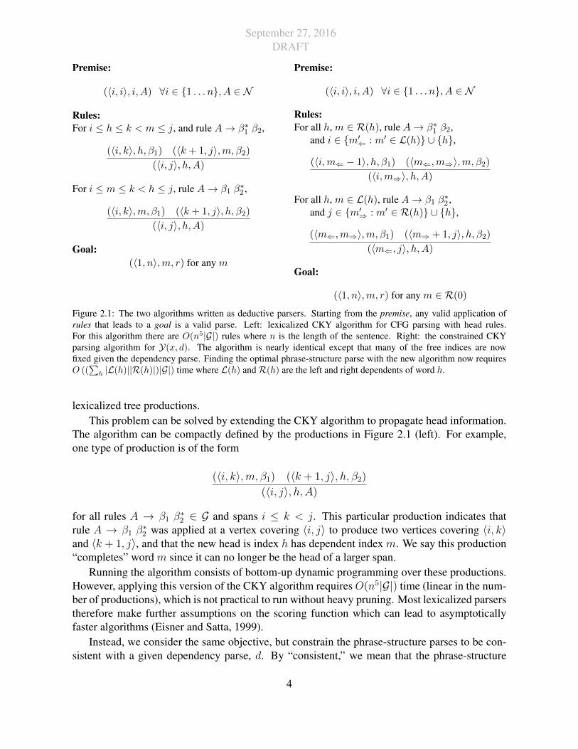
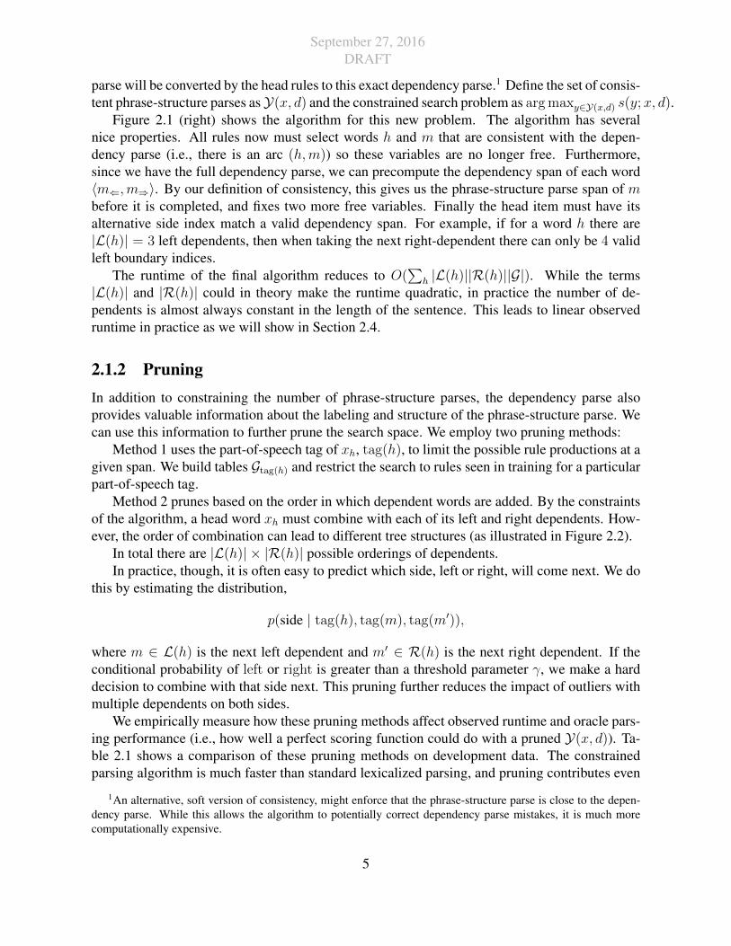
Figure 2.1: The two algorithms written as deductive parsers. Starting from the premise, any valid application ofrules that leads to a goal is a valid parse. Left: lexicalized CKY algorithm for CFG parsing with head rules.For this algorithm there are O(n5|G|) rules where n is the length of the sentence. Right: the constrained CKYparsing algorithm for Y(x, d). The algorithm is nearly identical except that many of the free indices are nowfixed given the dependency parse. Finding the optimal phrase-structure parse with the new algorithm now requiresO ((

∑h |L(h)||R(h)|)|G|) time where L(h) andR(h) are the left and right dependents of word h.

lexicalized tree productions.This problem can be solved by extending the CKY algorithm to propagate head information.

The algorithm can be compactly defined by the productions in Figure 2.1 (left). For example,one type of production is of the form

(〈i, k〉,m, β1) (〈k + 1, j〉, h, β2)(〈i, j〉, h, A)

for all rules A → β1 β∗2 ∈ G and spans i ≤ k < j. This particular production indicates that

rule A → β1 β∗2 was applied at a vertex covering 〈i, j〉 to produce two vertices covering 〈i, k〉

and 〈k + 1, j〉, and that the new head is index h has dependent index m. We say this production“completes” word m since it can no longer be the head of a larger span.

Running the algorithm consists of bottom-up dynamic programming over these productions.However, applying this version of the CKY algorithm requires O(n5|G|) time (linear in the num-ber of productions), which is not practical to run without heavy pruning. Most lexicalized parserstherefore make further assumptions on the scoring function which can lead to asymptoticallyfaster algorithms (Eisner and Satta, 1999).

Instead, we consider the same objective, but constrain the phrase-structure parses to be con-sistent with a given dependency parse, d. By “consistent,” we mean that the phrase-structure

4


parse will be converted by the head rules to this exact dependency parse.1 Define the set of consis-tent phrase-structure parses asY(x, d) and the constrained search problem as arg maxy∈Y(x,d) s(y;x, d).

Figure 2.1 (right) shows the algorithm for this new problem. The algorithm has severalnice properties. All rules now must select words h and m that are consistent with the depen-dency parse (i.e., there is an arc (h,m)) so these variables are no longer free. Furthermore,since we have the full dependency parse, we can precompute the dependency span of each word〈m⇐,m⇒〉. By our definition of consistency, this gives us the phrase-structure parse span of mbefore it is completed, and fixes two more free variables. Finally the head item must have itsalternative side index match a valid dependency span. For example, if for a word h there are|L(h)| = 3 left dependents, then when taking the next right-dependent there can only be 4 validleft boundary indices.

The runtime of the final algorithm reduces to O(∑

h |L(h)||R(h)||G|). While the terms|L(h)| and |R(h)| could in theory make the runtime quadratic, in practice the number of de-pendents is almost always constant in the length of the sentence. This leads to linear observedruntime in practice as we will show in Section 2.4.

2.1.2 PruningIn addition to constraining the number of phrase-structure parses, the dependency parse alsoprovides valuable information about the labeling and structure of the phrase-structure parse. Wecan use this information to further prune the search space. We employ two pruning methods:

Method 1 uses the part-of-speech tag of xh, tag(h), to limit the possible rule productions at agiven span. We build tables Gtag(h) and restrict the search to rules seen in training for a particularpart-of-speech tag.

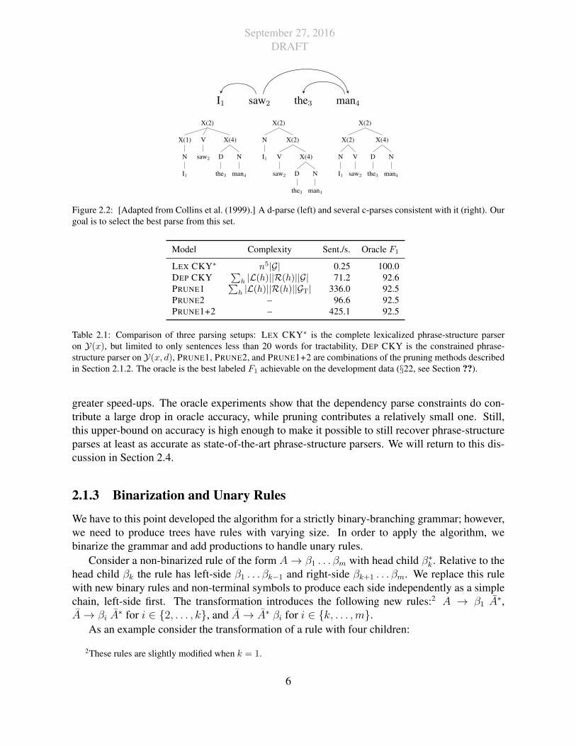
Method 2 prunes based on the order in which dependent words are added. By the constraintsof the algorithm, a head word xh must combine with each of its left and right dependents. How-ever, the order of combination can lead to different tree structures (as illustrated in Figure 2.2).

In total there are |L(h)| × |R(h)| possible orderings of dependents.In practice, though, it is often easy to predict which side, left or right, will come next. We do

this by estimating the distribution,

p(side | tag(h), tag(m), tag(m′)),

where m ∈ L(h) is the next left dependent and m′ ∈ R(h) is the next right dependent. If theconditional probability of left or right is greater than a threshold parameter γ, we make a harddecision to combine with that side next. This pruning further reduces the impact of outliers withmultiple dependents on both sides.

We empirically measure how these pruning methods affect observed runtime and oracle pars-ing performance (i.e., how well a perfect scoring function could do with a pruned Y(x, d)). Ta-ble 2.1 shows a comparison of these pruning methods on development data. The constrainedparsing algorithm is much faster than standard lexicalized parsing, and pruning contributes even

1An alternative, soft version of consistency, might enforce that the phrase-structure parse is close to the depen-dency parse. While this allows the algorithm to potentially correct dependency parse mistakes, it is much morecomputationally expensive.

5


I1 saw2 the3 man4

X(2)

X(4)

N

man4

D

the3

V

saw2

X(1)

N

I1

X(2)

X(2)

X(4)

N

man4

D

the3

V

saw2

N

I1

X(2)

X(4)

N

man4

D

the3

X(2)

V

saw2

N

I1

Figure 2.2: [Adapted from Collins et al. (1999).] A d-parse (left) and several c-parses consistent with it (right). Ourgoal is to select the best parse from this set.

Model Complexity Sent./s. Oracle F1

LEX CKY∗ n5|G| 0.25 100.0DEP CKY

∑h |L(h)||R(h)||G| 71.2 92.6

PRUNE1∑h |L(h)||R(h)||GT| 336.0 92.5

PRUNE2 – 96.6 92.5PRUNE1+2 – 425.1 92.5

Table 2.1: Comparison of three parsing setups: LEX CKY∗ is the complete lexicalized phrase-structure parseron Y(x), but limited to only sentences less than 20 words for tractability, DEP CKY is the constrained phrase-structure parser on Y(x, d), PRUNE1, PRUNE2, and PRUNE1+2 are combinations of the pruning methods describedin Section 2.1.2. The oracle is the best labeled F1 achievable on the development data (§22, see Section ??).

greater speed-ups. The oracle experiments show that the dependency parse constraints do con-tribute a large drop in oracle accuracy, while pruning contributes a relatively small one. Still,this upper-bound on accuracy is high enough to make it possible to still recover phrase-structureparses at least as accurate as state-of-the-art phrase-structure parsers. We will return to this dis-cussion in Section 2.4.

2.1.3 Binarization and Unary Rules

We have to this point developed the algorithm for a strictly binary-branching grammar; however,we need to produce trees have rules with varying size. In order to apply the algorithm, webinarize the grammar and add productions to handle unary rules.

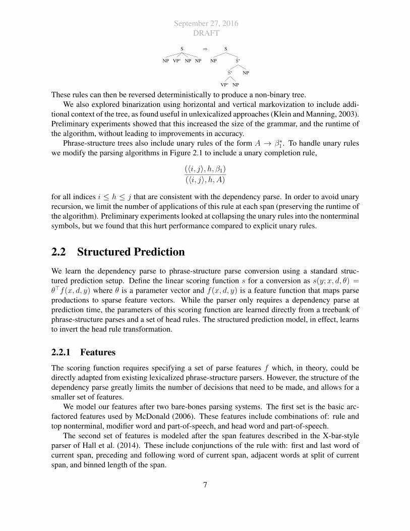
Consider a non-binarized rule of the form A→ β1 . . . βm with head child β∗k . Relative to thehead child βk the rule has left-side β1 . . . βk−1 and right-side βk+1 . . . βm. We replace this rulewith new binary rules and non-terminal symbols to produce each side independently as a simplechain, left-side first. The transformation introduces the following new rules:2 A → β1 A

∗,A→ βi A

∗ for i ∈ {2, . . . , k}, and A→ A∗ βi for i ∈ {k, . . . ,m}.As an example consider the transformation of a rule with four children:

2These rules are slightly modified when k = 1.

6


S

NPNPVP∗NP

⇒ S

S∗

NPS∗

NPVP∗

NP

These rules can then be reversed deterministically to produce a non-binary tree.We also explored binarization using horizontal and vertical markovization to include addi-

tional context of the tree, as found useful in unlexicalized approaches (Klein and Manning, 2003).Preliminary experiments showed that this increased the size of the grammar, and the runtime ofthe algorithm, without leading to improvements in accuracy.

Phrase-structure trees also include unary rules of the form A → β∗1 . To handle unary ruleswe modify the parsing algorithms in Figure 2.1 to include a unary completion rule,

(〈i, j〉, h, β1)(〈i, j〉, h, A)

for all indices i ≤ h ≤ j that are consistent with the dependency parse. In order to avoid unaryrecursion, we limit the number of applications of this rule at each span (preserving the runtime ofthe algorithm). Preliminary experiments looked at collapsing the unary rules into the nonterminalsymbols, but we found that this hurt performance compared to explicit unary rules.

2.2 Structured PredictionWe learn the dependency parse to phrase-structure parse conversion using a standard struc-tured prediction setup. Define the linear scoring function s for a conversion as s(y;x, d, θ) =θ>f(x, d, y) where θ is a parameter vector and f(x, d, y) is a feature function that maps parseproductions to sparse feature vectors. While the parser only requires a dependency parse atprediction time, the parameters of this scoring function are learned directly from a treebank ofphrase-structure parses and a set of head rules. The structured prediction model, in effect, learnsto invert the head rule transformation.

2.2.1 FeaturesThe scoring function requires specifying a set of parse features f which, in theory, could bedirectly adapted from existing lexicalized phrase-structure parsers. However, the structure of thedependency parse greatly limits the number of decisions that need to be made, and allows for asmaller set of features.

We model our features after two bare-bones parsing systems. The first set is the basic arc-factored features used by McDonald (2006). These features include combinations of: rule andtop nonterminal, modifier word and part-of-speech, and head word and part-of-speech.

The second set of features is modeled after the span features described in the X-bar-styleparser of Hall et al. (2014). These include conjunctions of the rule with: first and last word ofcurrent span, preceding and following word of current span, adjacent words at split of currentspan, and binned length of the span.

7


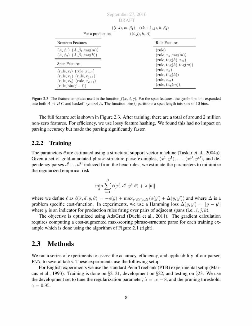
For a production(〈i, k〉,m, β1) (〈k + 1, j〉, h, β2)

(〈i, j〉, h, A)

Nonterm Features

(A, β1) (A, β1, tag(m))(A, β2) (A, β2, tag(h))

Span Features

(rule, xi) (rule, xi−1)(rule, xj) (rule, xj+1)(rule, xk) (rule, xk+1)(rule,bin(j − i))

Rule Features

(rule)(rule, xh, tag(m))(rule, tag(h), xm)(rule, tag(h), tag(m))(rule, xh)(rule, tag(h))(rule, xm)(rule, tag(m))

Figure 2.3: The feature templates used in the function f(x, d, y). For the span features, the symbol rule is expandedinto both A→ B C and backoff symbol A. The function bin(i) partitions a span length into one of 10 bins.

The full feature set is shown in Figure 2.3. After training, there are a total of around 2 millionnon-zero features. For efficiency, we use lossy feature hashing. We found this had no impact onparsing accuracy but made the parsing significantly faster.

2.2.2 TrainingThe parameters θ are estimated using a structural support vector machine (Taskar et al., 2004a).Given a set of gold-annotated phrase-structure parse examples, (x1, y1), . . . , (xD, yD), and de-pendency parses d1 . . . dD induced from the head rules, we estimate the parameters to minimizethe regularized empirical risk

minθ

D∑

i=1

`(xi, di, yi, θ) + λ||θ||1

where we define ` as `(x, d, y, θ) = −s(y) + maxy′∈Y(x,d) (s(y′) + ∆(y, y′)) and where ∆ is aproblem specific cost-function. In experiments, we use a Hamming loss ∆(y, y′) = |y − y′|where y is an indicator for production rules firing over pairs of adjacent spans (i.e., i, j, k).

The objective is optimized using AdaGrad (Duchi et al., 2011). The gradient calculationrequires computing a cost-augmented max-scoring phrase-structure parse for each training ex-ample which is done using the algorithm of Figure 2.1 (right).

2.3 MethodsWe ran a series of experiments to assess the accuracy, efficiency, and applicability of our parser,PAD, to several tasks. These experiments use the following setup.

For English experiments we use the standard Penn Treebank (PTB) experimental setup (Mar-cus et al., 1993). Training is done on §2–21, development on §22, and testing on §23. We usethe development set to tune the regularization parameter, λ = 1e− 8, and the pruning threshold,γ = 0.95.

8


For Chinese experiments, we use version 5.1 of the Penn Chinese Treebank 5.1 (CTB) (Xueet al., 2005). We followed previous work and used articles 001–270 and 440–1151 for training,301–325 for development, and 271–300 for test. We also use the development set to tune theregularization parameter, λ = 1e− 3.

Part-of-speech tagging is performed for all models using TurboTagger (Martins et al., 2013).Prior to training the dependency parser, the training sections are automatically processed using10-fold jackknifing (Collins and Koo, 2005) for both dependency and phrase structure trees. Zhuet al. (2013) found this simple technique gives an improvement to dependency accuracy of 0.4%on English and 2.0% on Chinese in their system.

During training, we use the dependency parses induced by the head rules from the goldphrase-structure parses as constraints. There is a slight mismatch here with test, since thesedependency parses are guaranteed to be consistent with the target phrase-structure parse. Wealso experimented with using 10-fold jacknifing of the dependency parser during training toproduce more realistic parses; however, we found that this hurt performance of the parser.

Unless otherwise noted, in English the test dependency parsing is done using the RedShiftimplementation3 of the parser of Zhang and Nivre (2011), trained to follow the conventions ofCollins head rules (Collins, 2003). This parser is a transition-based beam search parser, and thesize of the beam k controls a speed/accuracy trade-off. By default we use a beam of k = 16.We found that dependency labels have a significant impact on the performance of the RedShiftparser, but not on English dependency conversion. We therefore train a labeled parser, but discardthe labels.

For Chinese, we use the head rules compiled by Ding and Palmer (2005)4. For this data-setwe trained the dependency parser using the YaraParser implementation5 of the parser of Zhangand Nivre (2011), because it has a better Chinese implementation. We use a beam of k = 64. Inexperiments, we found that Chinese labels were quite helpful, and added four additional featurestemplates conjoining the label with the non-terminals of a rule.

Evaluation for phrase-structure parses is performed using the evalb6 script with the standardsetup. We report labeled F1 scores as well as recall and precision. For dependency parsing, wereport unlabeled accuracy score (UAS).

We implemented the grammar binarization, head rules, and pruning tables in Python, andthe parser, features, and training in C++. Experiments are performed on a Lenovo ThinkCentredesktop computer with 32GB of memory and Core i7-3770 3.4GHz 8M cache CPU.

2.4 Experiments

We ran experiments to assess the accuracy of the method, its runtime efficiency, the effect ofdependency parsing accuracy, and the effect of the amount of annotated phrase-structure data.

3https://github.com/syllog1sm/redshift4http://stp.lingfil.uu.se/˜nivre/research/chn_headrules.txt5https://github.com/yahoo/YaraParser6http://nlp.cs.nyu.edu/evalb

9

https://github.com/syllog1sm/redshift

http://stp.lingfil.uu.se/~nivre/research/chn_headrules.txt

https://github.com/yahoo/YaraParser

http://nlp.cs.nyu.edu/evalb


PTB §23Model F1 Sent./s.

Charniak (2000) 89.5 –Stanford PCFG (2003) 85.5 5.3Petrov (2007) 90.1 8.6Zhu (2013) 90.3 39.0Carreras (2008) 91.1 –

CJ Reranking (2005) 91.5 4.3Stanford RNN (2013) 90.0 2.8

PAD 90.4 34.3PAD (Pruned) 90.3 58.6

CTBModel F1

Charniak (2000) 80.8Bikel (2004) 80.6Petrov (2007) 83.3Zhu (2013) 83.2

PAD 82.4

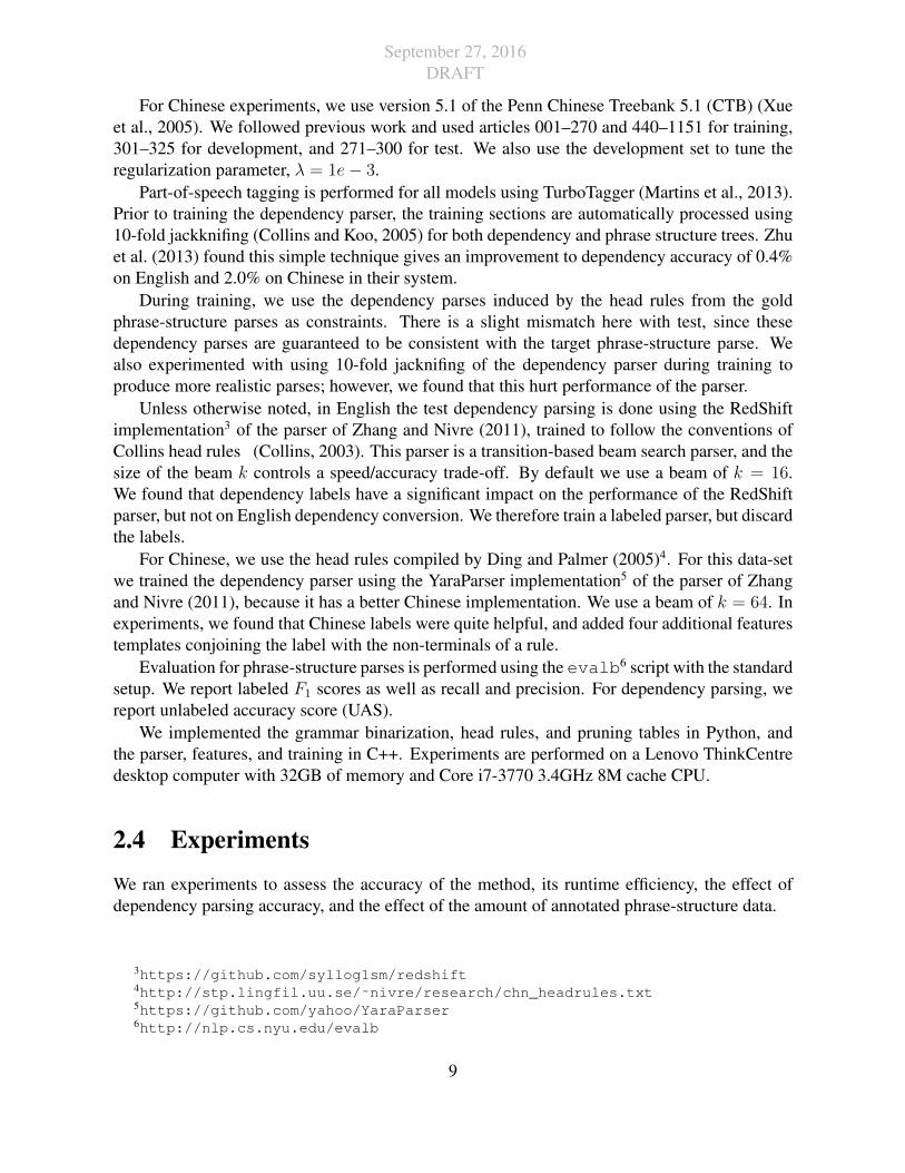
Table 2.2: Accuracy and speed on PTB §23 and CTB 5.1 test split. Comparisons are to state-of-the-art non-rerankingsupervised phrase-structure parsers (Charniak, 2000; Klein and Manning, 2003; Petrov and Klein, 2007; Carreraset al., 2008; Zhu et al., 2013; Bikel, 2004), and semi-supervised and reranking parsers (Charniak and Johnson, 2005;Socher et al., 2013).

Model UAS F1 Sent./s. Oracle

MALTPARSER 89.7 85.5 240.7 87.8RS-K1 90.1 86.6 233.9 87.6RS-K4 92.5 90.1 151.3 91.5RS-K16 93.1 90.6 58.6 92.5YARA-K1 89.7 85.3 1265.8 86.7YARA-K16 92.9 89.8 157.5 91.7YARA-K32 93.1 90.4 48.3 92.0YARA-K64 93.1 90.5 47.3 92.2TP-BASIC 92.8 88.9 132.8 90.8TP-STANDARD 93.3 90.9 27.2 92.6TP-FULL 93.5 90.8 13.2 92.9

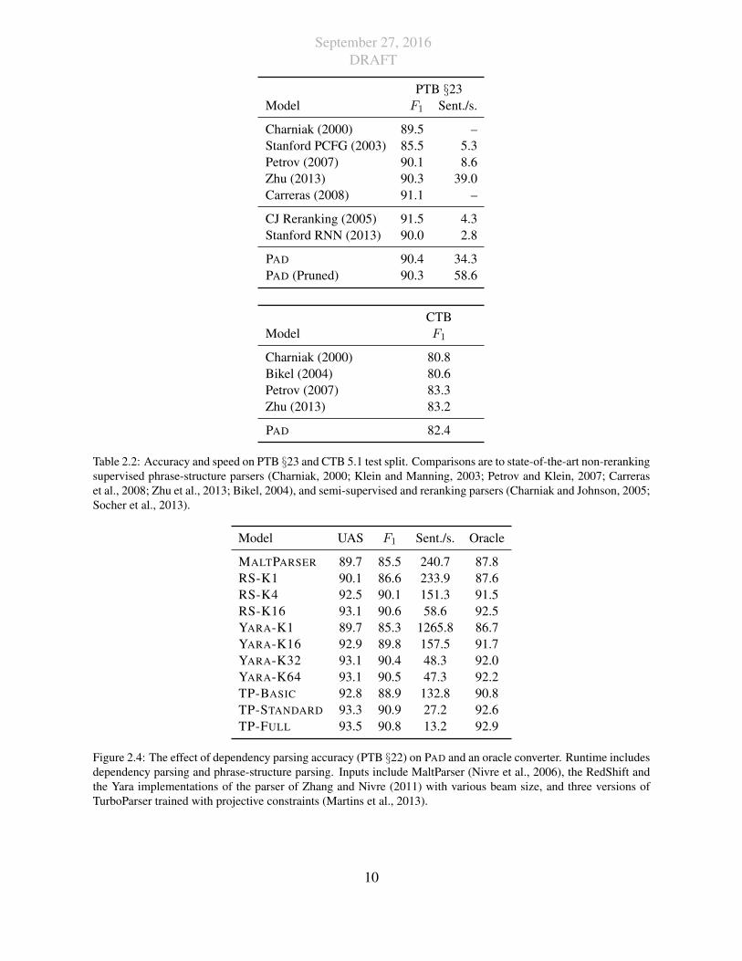
Figure 2.4: The effect of dependency parsing accuracy (PTB §22) on PAD and an oracle converter. Runtime includesdependency parsing and phrase-structure parsing. Inputs include MaltParser (Nivre et al., 2006), the RedShift andthe Yara implementations of the parser of Zhang and Nivre (2011) with various beam size, and three versions ofTurboParser trained with projective constraints (Martins et al., 2013).

10


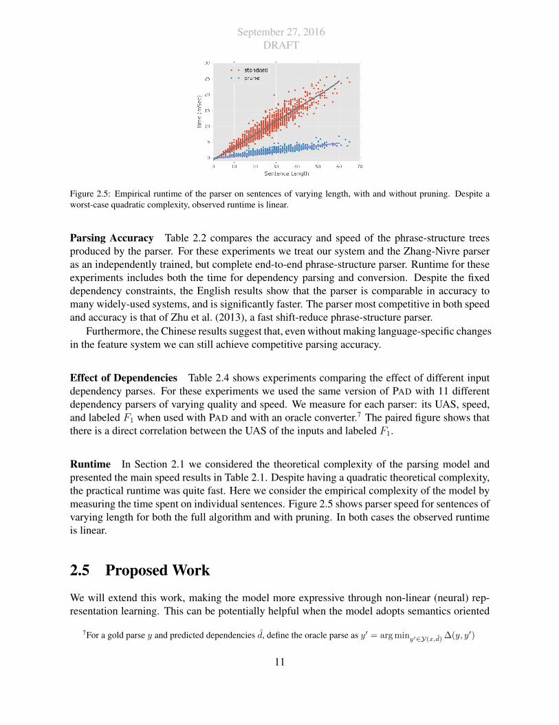
Figure 2.5: Empirical runtime of the parser on sentences of varying length, with and without pruning. Despite aworst-case quadratic complexity, observed runtime is linear.

Parsing Accuracy Table 2.2 compares the accuracy and speed of the phrase-structure treesproduced by the parser. For these experiments we treat our system and the Zhang-Nivre parseras an independently trained, but complete end-to-end phrase-structure parser. Runtime for theseexperiments includes both the time for dependency parsing and conversion. Despite the fixeddependency constraints, the English results show that the parser is comparable in accuracy tomany widely-used systems, and is significantly faster. The parser most competitive in both speedand accuracy is that of Zhu et al. (2013), a fast shift-reduce phrase-structure parser.

Furthermore, the Chinese results suggest that, even without making language-specific changesin the feature system we can still achieve competitive parsing accuracy.

Effect of Dependencies Table 2.4 shows experiments comparing the effect of different inputdependency parses. For these experiments we used the same version of PAD with 11 differentdependency parsers of varying quality and speed. We measure for each parser: its UAS, speed,and labeled F1 when used with PAD and with an oracle converter.7 The paired figure shows thatthere is a direct correlation between the UAS of the inputs and labeled F1.

Runtime In Section 2.1 we considered the theoretical complexity of the parsing model andpresented the main speed results in Table 2.1. Despite having a quadratic theoretical complexity,the practical runtime was quite fast. Here we consider the empirical complexity of the model bymeasuring the time spent on individual sentences. Figure 2.5 shows parser speed for sentences ofvarying length for both the full algorithm and with pruning. In both cases the observed runtimeis linear.

2.5 Proposed Work

We will extend this work, making the model more expressive through non-linear (neural) rep-resentation learning. This can be potentially helpful when the model adopts semantics oriented

7For a gold parse y and predicted dependencies d, define the oracle parse as y′ = arg miny′∈Y(x,d) ∆(y, y′)

11


head-rules (e.g. Stanford head rules (De Marneffe and Manning, 2008)) where the context be-comes more non-local.

Soft structural constraints in the model can be understood as a regularizer of learned repre-sentations (Zhang and Weiss, 2016). We will extend the previous work by exploring this generalapproach to incorporating the structural information in neural models.

12


Chapter 3

Segmental Recurrent Neural Networks

Our prior work (Kong et al., 2015a; Lu et al., 2016) introduces segmental recurrent neuralnetworks (SRNNs) which define, given an input sequence, a joint probability distribution oversegmentations of the input and labelings of the segments. Representations of the input segments(i.e., contiguous subsequences of the input) are computed by encoding their constituent tokensusing bidirectional recurrent neural nets, and these “segment embeddings” are used to definecompatibility scores with output labels. These local compatibility scores are integrated using aglobal semi-Markov conditional random field. Both fully supervised training—in which segmentboundaries and labels are observed—as well as partially supervised training—in which segmentboundaries are latent—are straightforward. Experiments show that, compared to models thatdo not explicitly represent segments such as BIO tagging schemes and connectionist temporalclassification (CTC), SRNNs obtain substantially higher accuracies.

3.1 Model

Given a sequence of input observations x = 〈x1, x2, . . . , x|x|〉 with length |x|, a segmentalrecurrent neural network (SRNN) defines a joint distribution p(y, z | x) over a sequence oflabeled segments each of which is characterized by a duration (zi ∈ Z+) and label (yi ∈ Y ).The segment durations constrained such that

∑|z|i=1 zi = |x|. The length of the output sequence

|y| = |z| is a random variable, and |y| ≤ |x| with probability 1. We write the starting time ofsegment i as si = 1 +

∑j<i zj .

To motivate our model form, we state several desiderata. First, we are interested in thefollowing prediction problem,

y∗ = arg maxy

p(y | x) = arg maxy

∑

z

p(y, z | x) ≈ arg maxy

maxz

p(y, z | x). (3.1)

Note the use of joint maximization over y and z as a computationally tractable substitute formarginalizing out z; this is commonly done in natural language processing.

Second, for problems where the explicit durations observations are unavailable at trainingtime and are inferred as a latent variable, we must be able to use a marginal likelihood training

13


criterion,

L = − log p(y | x) = − log∑

z

p(y, z | x). (3.2)

In Eqs. 3.1 and 3.2, the conditional probability of the labeled segment sequence is (assuming kthorder dependencies on y):

p(y, z | x) =1

Z(x)

|y|∏

i=1

exp f(yi−k:i, zi, x) (3.3)

where Z(x) is an appropriate normalization function. To ensure the expressiveness of f and thecomputational efficiency of the maximization and marginalization problems in Eqs. 3.1 and 3.2,we use the following definition of f ,

f(yi−k:i, zi, xsi:si+zi−1) = w>φ(V[gy(yi−k); . . . ; gy(yi); gz(zi);−−→RNN(csi:si+zi−1);

←−−RNN(csi:si+zi−1)] + a) + b

(3.4)

where−−→RNN(csi:si+zi−1) is a recurrent neural network that computes the forward segment em-

bedding by “encoding” the zi-length subsequence of x starting at index si,1 and←−−RNN computes

the reverse segment embedding (i.e., traversing the sequence in reverse order), and gy and gzare functions which map the label candidate y and segmentation duration z into a vector repre-sentation. The notation [a;b; c] denotes vector concatenation. Finally, the concatenated segmentduration, label candidates and segment embedding are passed through a affine transformationlayer parameterized by V and a and a nonlinear activation function φ (e.g., tanh), and a dotproduct with a vector w and addition by scalar b computes the log potential for the clique. Ourproposed model is equivalent to a semi-Markov conditional random field with local featurescomputed using neural networks. Figure 3.1 shows the model graphically.

We chose bidirectional LSTMs (Graves and Schmidhuber, 2005) as the implementation ofthe RNNs in Eq. 3.4. LSTMs (Hochreiter and Schmidhuber, 1997) are a popular variant ofRNNs which have been seen successful in many representation learning problems (Graves andJaitly, 2014; Karpathy and Fei-Fei, 2015). Bidirectional LSTMs enable effective computation forembedings in both directions and are known to be good at preserving long distance dependencies,and hence are well-suited for our task.

3.2 Inference with Dynamic ProgrammingWe are interested in three inference problems: (i) finding the most probable segmentation/labelingfor a model given a sequence x; (ii) evaluating the partition function Z(x); and (iii) computingthe posterior marginal Z(x,y), which sums over all segmentations compatible with a reference

1Rather than directly reading the xi’s, each token is represented as the concatenation, ci, of a forward andbackward over the sequence of raw inputs. This permits tokens to be sensitive to the contexts they occur in, and thisis standardly used with neural net sequence labeling models (Graves et al., 2006b).

14


x1 x2 x3 x4 x5 x6

(

(

Enco

der B

iRN

NSe

gmen

tatio

n/La

belin

g M

odel

x1 x2x1 x2x1 x2x1 x2x1x1 x2x1

c1 c2 c3 c4 c5 c6

z1 z2 z3

y1 y2 y3

x1 x2 x3 x4 x5 x6

�!h 1,3

�!h 4,5

�!h 6,6

�h 6,6

�h 4,5

�h 1,3

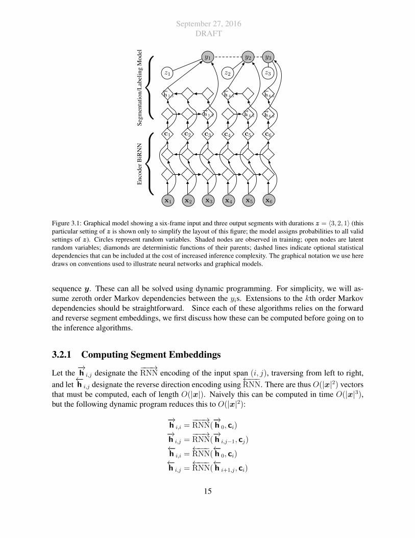
Figure 3.1: Graphical model showing a six-frame input and three output segments with durations z = 〈3, 2, 1〉 (thisparticular setting of z is shown only to simplify the layout of this figure; the model assigns probabilities to all validsettings of z). Circles represent random variables. Shaded nodes are observed in training; open nodes are latentrandom variables; diamonds are deterministic functions of their parents; dashed lines indicate optional statisticaldependencies that can be included at the cost of increased inference complexity. The graphical notation we use heredraws on conventions used to illustrate neural networks and graphical models.

sequence y. These can all be solved using dynamic programming. For simplicity, we will as-sume zeroth order Markov dependencies between the yis. Extensions to the kth order Markovdependencies should be straightforward. Since each of these algorithms relies on the forwardand reverse segment embeddings, we first discuss how these can be computed before going on tothe inference algorithms.

3.2.1 Computing Segment Embeddings

Let the−→h i,j designate the

−−−→RNN encoding of the input span (i, j), traversing from left to right,

and let←−h i,j designate the reverse direction encoding using

←−−−RNN. There are thus O(|x|2) vectors

that must be computed, each of length O(|x|). Naively this can be computed in time O(|x|3),but the following dynamic program reduces this to O(|x|2):

−→h i,i =

−−−→RNN(

−→h 0, ci)

−→h i,j =

−−−→RNN(

−→h i,j−1, cj)

←−h i,i =

←−−−RNN(

←−h 0, ci)

←−h i,j =

←−−−RNN(

←−h i+1,j, ci)

15


The algorithm is executed by initializing in the values on the diagonal (representing segmentsof length 1) and then inductively filling out the rest of the matrix. In practice, we often canput a upper bound for the length of a eligible segment thus reducing the complexity of runtimeto O(|x|). This savings can be substantial for very long sequences (e.g., those encountered inspeech recognition).

3.2.2 Computing the most probable segmentation/labeling and Z(x)

For the input sequence x, there are 2|x|−1 possible segmentations and O(|Y ||x|) different la-belings of these segments, making exhaustive computation entirely infeasible. Fortunately, thepartition function Z(x) may be computed in polynomial time with the following dynamic pro-gram:

α0 = 1

αj =∑

i<j

αi ×∑

y∈Y

(expw>φ(V[gy(y); gz(zi);

−−→RNN(csi:si+zi−1);


).

After computing these values, Z(x) = α|x|. By changing the summations to a max operators(and storing the corresponding arg max values), the maximal a posteriori segmentation/labelingcan be computed.

Both the partition function evaluation and the search for the MAP outputs run in timeO(|x|2 ·|Y |) with this dynamic program. Adding nth order Markov dependencies between the yis addsrequires additional information in each state and increases the time and space requirements by afactor of O(|Y |n). However, this may be tractable for small |Y | and n.

Avoiding overflow. Since this dynamic program sums over exponentially many segmentationsand labelings, the values in the αi chart can become very large. Thus, to avoid issues withoverflow, computations of the αi’s must be carried out in log space.2

3.2.3 Computing Z(x,y)

To compute the posterior marginal Z(x,y), it is necessary to sum over all segmentations that arecompatible with a label sequence y given an input sequence x. To do so requires only a minormodification of the previous dynamic program to track how much of the reference label sequencey has been consumed. We introduce the variable m as the index into y for this purpose. The

2An alternative strategy for avoiding overflow in similar dynamic programs is to rescale the forward summationsat each time step (Rabiner, 1989; Graves et al., 2006b). Unfortunately, in a semi-Markov architecture each term inαi sums over different segmentations (e.g., the summation for α2 will have contain some terms that include α1 andsome terms that include only α0), which means there are no common factors, making this strategy inapplicable.

16


modified recurrences are:

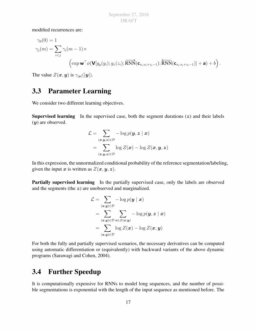
γ0(0) = 1

γj(m) =∑

i<j

γi(m− 1)×(

expw>φ(V[gy(yi); gz(zi);−−→RNN(csi:si+zi−1);


).

The value Z(x,y) is γ|x|(|y|).

3.3 Parameter LearningWe consider two different learning objectives.

Supervised learning In the supervised case, both the segment durations (z) and their labels(y) are observed.

L =∑

(x,y,z)∈D

− log p(y, z | x)

=∑

(x,y,z)∈D

logZ(x)− logZ(x,y, z)

In this expression, the unnormalized conditional probability of the reference segmentation/labeling,given the input x is written as Z(x,y, z).

Partially supervised learning In the partially supervised case, only the labels are observedand the segments (the z) are unobserved and marginalized.

L =∑

(x,y)∈D

− log p(y | x)

=∑

(x,y)∈D

∑

z∈Z(x,y)

− log p(y, z | x)

=∑

(x,y)∈D

logZ(x)− logZ(x,y)

For both the fully and partially supervised scenarios, the necessary derivatives can be computedusing automatic differentiation or (equivalently) with backward variants of the above dynamicprograms (Sarawagi and Cohen, 2004).

3.4 Further SpeedupIt is computationally expensive for RNNs to model long sequences, and the number of possi-ble segmentations is exponential with the length of the input sequence as mentioned before. The

17


x1 x2 x3 x4· · ·

x1 x2 x3 x4· · ·

a) concatenate / add

b) skip

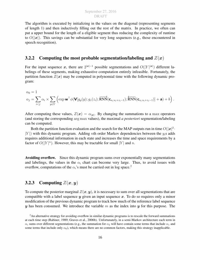
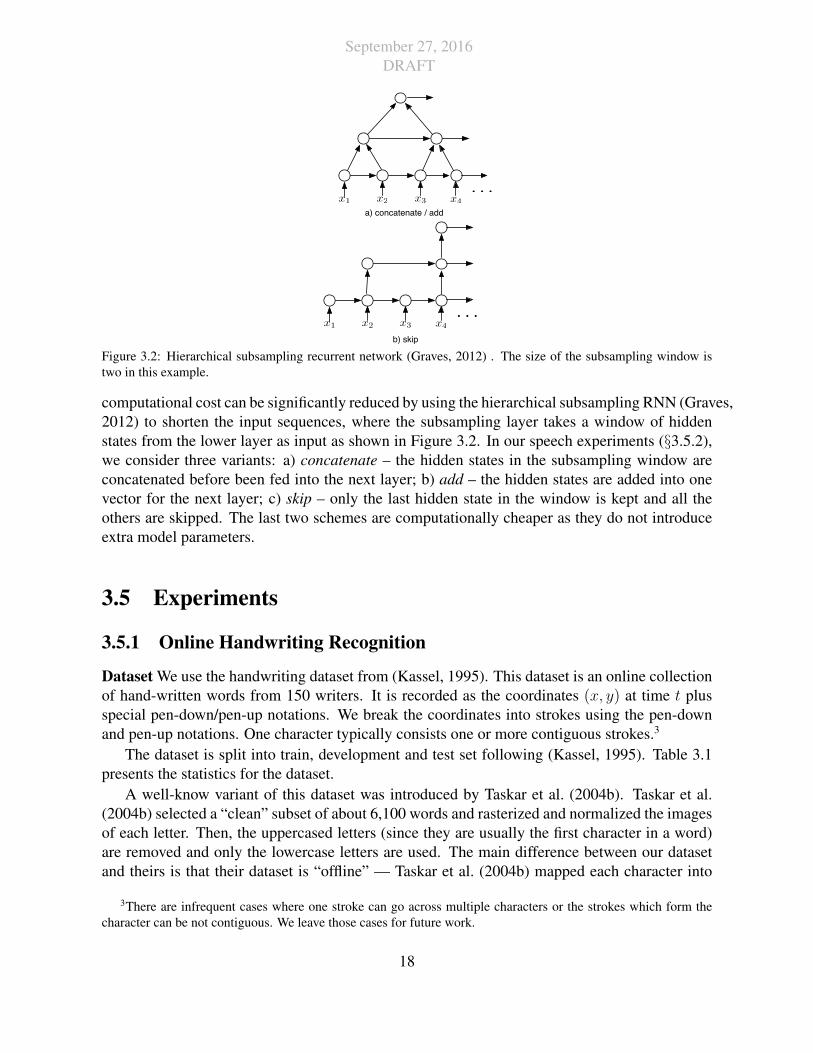
Figure 3.2: Hierarchical subsampling recurrent network (Graves, 2012) . The size of the subsampling window istwo in this example.

computational cost can be significantly reduced by using the hierarchical subsampling RNN (Graves,2012) to shorten the input sequences, where the subsampling layer takes a window of hiddenstates from the lower layer as input as shown in Figure 3.2. In our speech experiments (§3.5.2),we consider three variants: a) concatenate – the hidden states in the subsampling window areconcatenated before been fed into the next layer; b) add – the hidden states are added into onevector for the next layer; c) skip – only the last hidden state in the window is kept and all theothers are skipped. The last two schemes are computationally cheaper as they do not introduceextra model parameters.

3.5 Experiments

3.5.1 Online Handwriting Recognition

Dataset We use the handwriting dataset from (Kassel, 1995). This dataset is an online collectionof hand-written words from 150 writers. It is recorded as the coordinates (x, y) at time t plusspecial pen-down/pen-up notations. We break the coordinates into strokes using the pen-downand pen-up notations. One character typically consists one or more contiguous strokes.3

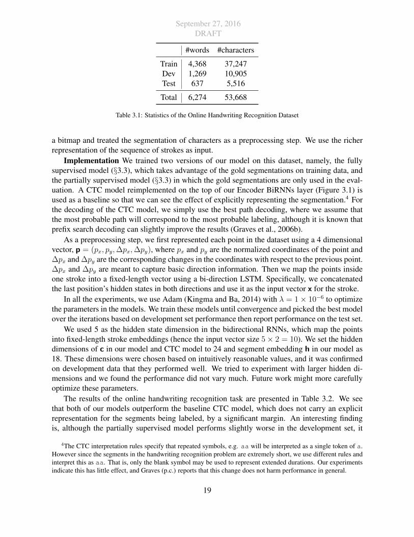
The dataset is split into train, development and test set following (Kassel, 1995). Table 3.1presents the statistics for the dataset.

A well-know variant of this dataset was introduced by Taskar et al. (2004b). Taskar et al.(2004b) selected a “clean” subset of about 6,100 words and rasterized and normalized the imagesof each letter. Then, the uppercased letters (since they are usually the first character in a word)are removed and only the lowercase letters are used. The main difference between our datasetand theirs is that their dataset is “offline” — Taskar et al. (2004b) mapped each character into

3There are infrequent cases where one stroke can go across multiple characters or the strokes which form thecharacter can be not contiguous. We leave those cases for future work.

18


#words #characters

Train 4,368 37,247Dev 1,269 10,905Test 637 5,516

Total 6,274 53,668

Table 3.1: Statistics of the Online Handwriting Recognition Dataset

a bitmap and treated the segmentation of characters as a preprocessing step. We use the richerrepresentation of the sequence of strokes as input.

Implementation We trained two versions of our model on this dataset, namely, the fullysupervised model (§3.3), which takes advantage of the gold segmentations on training data, andthe partially supervised model (§3.3) in which the gold segmentations are only used in the eval-uation. A CTC model reimplemented on the top of our Encoder BiRNNs layer (Figure 3.1) isused as a baseline so that we can see the effect of explicitly representing the segmentation.4 Forthe decoding of the CTC model, we simply use the best path decoding, where we assume thatthe most probable path will correspond to the most probable labeling, although it is known thatprefix search decoding can slightly improve the results (Graves et al., 2006b).

As a preprocessing step, we first represented each point in the dataset using a 4 dimensionalvector, p = (px, py,∆px,∆py), where px and py are the normalized coordinates of the point and∆px and ∆py are the corresponding changes in the coordinates with respect to the previous point.∆px and ∆py are meant to capture basic direction information. Then we map the points insideone stroke into a fixed-length vector using a bi-direction LSTM. Specifically, we concatenatedthe last position’s hidden states in both directions and use it as the input vector x for the stroke.

In all the experiments, we use Adam (Kingma and Ba, 2014) with λ = 1× 10−6 to optimizethe parameters in the models. We train these models until convergence and picked the best modelover the iterations based on development set performance then report performance on the test set.

We used 5 as the hidden state dimension in the bidirectional RNNs, which map the pointsinto fixed-length stroke embeddings (hence the input vector size 5× 2 = 10). We set the hiddendimensions of c in our model and CTC model to 24 and segment embedding h in our model as18. These dimensions were chosen based on intuitively reasonable values, and it was confirmedon development data that they performed well. We tried to experiment with larger hidden di-mensions and we found the performance did not vary much. Future work might more carefullyoptimize these parameters.

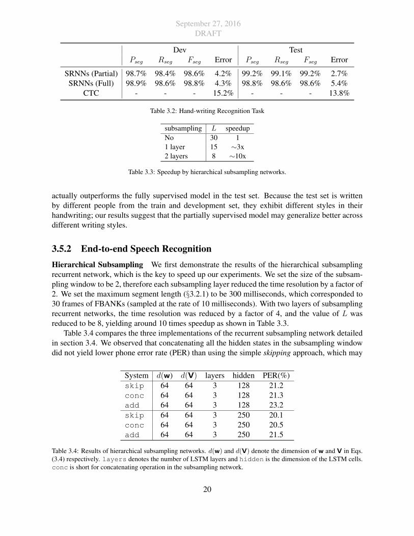
The results of the online handwriting recognition task are presented in Table 3.2. We seethat both of our models outperform the baseline CTC model, which does not carry an explicitrepresentation for the segments being labeled, by a significant margin. An interesting findingis, although the partially supervised model performs slightly worse in the development set, it

4The CTC interpretation rules specify that repeated symbols, e.g. aa will be interpreted as a single token of a.However since the segments in the handwriting recognition problem are extremely short, we use different rules andinterpret this as aa. That is, only the blank symbol may be used to represent extended durations. Our experimentsindicate this has little effect, and Graves (p.c.) reports that this change does not harm performance in general.

19


Dev TestPseg Rseg Fseg Error Pseg Rseg Fseg Error

SRNNs (Partial) 98.7% 98.4% 98.6% 4.2% 99.2% 99.1% 99.2% 2.7%SRNNs (Full) 98.9% 98.6% 98.8% 4.3% 98.8% 98.6% 98.6% 5.4%

CTC - - - 15.2% - - - 13.8%

Table 3.2: Hand-writing Recognition Task

subsampling L speedupNo 30 11 layer 15 ∼3x2 layers 8 ∼10x

Table 3.3: Speedup by hierarchical subsampling networks.

actually outperforms the fully supervised model in the test set. Because the test set is writtenby different people from the train and development set, they exhibit different styles in theirhandwriting; our results suggest that the partially supervised model may generalize better acrossdifferent writing styles.

3.5.2 End-to-end Speech RecognitionHierarchical Subsampling We first demonstrate the results of the hierarchical subsamplingrecurrent network, which is the key to speed up our experiments. We set the size of the subsam-pling window to be 2, therefore each subsampling layer reduced the time resolution by a factor of2. We set the maximum segment length (§3.2.1) to be 300 milliseconds, which corresponded to30 frames of FBANKs (sampled at the rate of 10 milliseconds). With two layers of subsamplingrecurrent networks, the time resolution was reduced by a factor of 4, and the value of L wasreduced to be 8, yielding around 10 times speedup as shown in Table 3.3.

Table 3.4 compares the three implementations of the recurrent subsampling network detailedin section 3.4. We observed that concatenating all the hidden states in the subsampling windowdid not yield lower phone error rate (PER) than using the simple skipping approach, which may

System d(w) d(V) layers hidden PER(%)skip 64 64 3 128 21.2conc 64 64 3 128 21.3add 64 64 3 128 23.2skip 64 64 3 250 20.1conc 64 64 3 250 20.5add 64 64 3 250 21.5

Table 3.4: Results of hierarchical subsampling networks. d(w) and d(V) denote the dimension of w and V in Eqs.(3.4) respectively. layers denotes the number of LSTM layers and hidden is the dimension of the LSTM cells.conc is short for concatenating operation in the subsampling network.

20


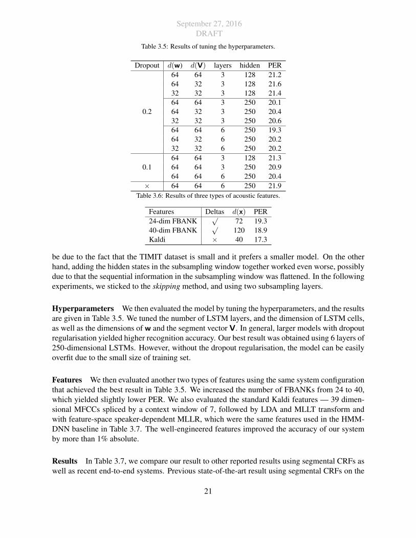
Table 3.5: Results of tuning the hyperparameters.

Dropout d(w) d(V) layers hidden PER64 64 3 128 21.264 32 3 128 21.632 32 3 128 21.464 64 3 250 20.1

0.2 64 32 3 250 20.432 32 3 250 20.664 64 6 250 19.364 32 6 250 20.232 32 6 250 20.264 64 3 128 21.3

0.1 64 64 3 250 20.964 64 6 250 20.4

× 64 64 6 250 21.9Table 3.6: Results of three types of acoustic features.

Features Deltas d(x) PER24-dim FBANK

√72 19.3

40-dim FBANK√

120 18.9Kaldi × 40 17.3

be due to the fact that the TIMIT dataset is small and it prefers a smaller model. On the otherhand, adding the hidden states in the subsampling window together worked even worse, possiblydue to that the sequential information in the subsampling window was flattened. In the followingexperiments, we sticked to the skipping method, and using two subsampling layers.

Hyperparameters We then evaluated the model by tuning the hyperparameters, and the resultsare given in Table 3.5. We tuned the number of LSTM layers, and the dimension of LSTM cells,as well as the dimensions of w and the segment vector V. In general, larger models with dropoutregularisation yielded higher recognition accuracy. Our best result was obtained using 6 layers of250-dimensional LSTMs. However, without the dropout regularisation, the model can be easilyoverfit due to the small size of training set.

Features We then evaluated another two types of features using the same system configurationthat achieved the best result in Table 3.5. We increased the number of FBANKs from 24 to 40,which yielded slightly lower PER. We also evaluated the standard Kaldi features — 39 dimen-sional MFCCs spliced by a context window of 7, followed by LDA and MLLT transform andwith feature-space speaker-dependent MLLR, which were the same features used in the HMM-DNN baseline in Table 3.7. The well-engineered features improved the accuracy of our systemby more than 1% absolute.

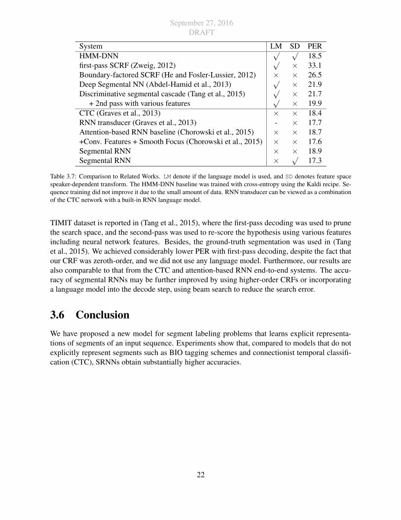
Results In Table 3.7, we compare our result to other reported results using segmental CRFs aswell as recent end-to-end systems. Previous state-of-the-art result using segmental CRFs on the

21


System LM SD PERHMM-DNN

√ √18.5

first-pass SCRF (Zweig, 2012)√ × 33.1

Boundary-factored SCRF (He and Fosler-Lussier, 2012) × × 26.5Deep Segmental NN (Abdel-Hamid et al., 2013)

√ × 21.9Discriminative segmental cascade (Tang et al., 2015)

√ × 21.7+ 2nd pass with various features

√ × 19.9CTC (Graves et al., 2013) × × 18.4RNN transducer (Graves et al., 2013) - × 17.7Attention-based RNN baseline (Chorowski et al., 2015) × × 18.7+Conv. Features + Smooth Focus (Chorowski et al., 2015) × × 17.6Segmental RNN × × 18.9Segmental RNN × √

17.3

Table 3.7: Comparison to Related Works. LM denote if the language model is used, and SD denotes feature spacespeaker-dependent transform. The HMM-DNN baseline was trained with cross-entropy using the Kaldi recipe. Se-quence training did not improve it due to the small amount of data. RNN transducer can be viewed as a combinationof the CTC network with a built-in RNN language model.

TIMIT dataset is reported in (Tang et al., 2015), where the first-pass decoding was used to prunethe search space, and the second-pass was used to re-score the hypothesis using various featuresincluding neural network features. Besides, the ground-truth segmentation was used in (Tanget al., 2015). We achieved considerably lower PER with first-pass decoding, despite the fact thatour CRF was zeroth-order, and we did not use any language model. Furthermore, our results arealso comparable to that from the CTC and attention-based RNN end-to-end systems. The accu-racy of segmental RNNs may be further improved by using higher-order CRFs or incorporatinga language model into the decode step, using beam search to reduce the search error.

3.6 ConclusionWe have proposed a new model for segment labeling problems that learns explicit representa-tions of segments of an input sequence. Experiments show that, compared to models that do notexplicitly represent segments such as BIO tagging schemes and connectionist temporal classifi-cation (CTC), SRNNs obtain substantially higher accuracies.

22


Chapter 4

Modeling the Compositionality in CCGSupertagging

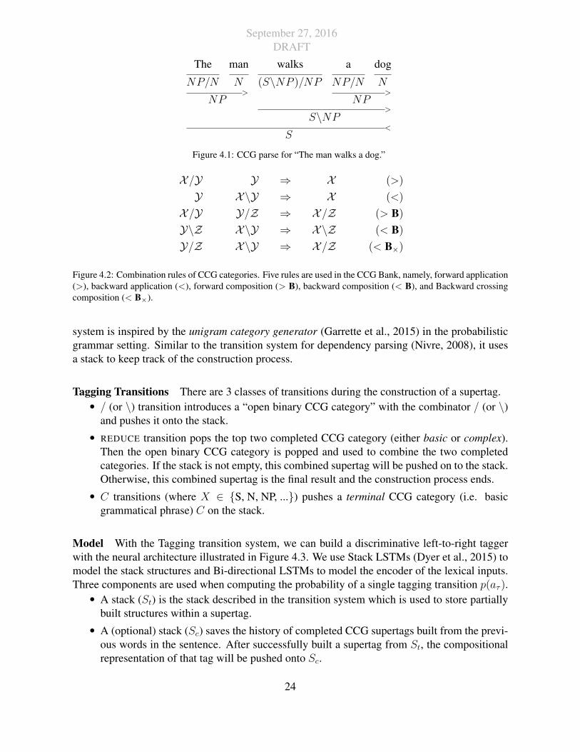
Combinatory categorical grammar (CCG) is widely used in semantic parsing, and parsing with itis very fast, especially if a good (probabilistic) tagger is available (Lewis and Steedman, 2014a;Lee et al., 2016). An example of a parse tree of CCG is shown in Figure 4.1 Each lexical tokenis associated with a structured category (i.e., supertag) in CCG. The number of lexical categoriesis unbounded in theory. In practice, previous work (Lewis and Steedman, 2014a; Xu et al.,2015b; Lewis and Steedman, 2014b, inter alia) use over 400 supertags and treat them as discretecategories, while Penn Treebank (Marcus et al., 1993) only has 50 predefined POS tags.

We propose to model the compositionality (§4.1) both inside these tags (intra-) and betweenthese tags (inter-). Previous works suggests that explicit modeling of such information can leadsto better accuracy (Srikumar and Manning, 2014) and less supervision (Garrette et al., 2015).

4.1 CCG and SupertaggingA CCG category (C) follows the recursive definition:

C → {S, N, NP, ...}C → {C/C, C\C}

It can either be an atomic category representing basic grammatical phrase (e.g. S, N, NP) ora complex category formed from the combination of two categories by one of the two slashoperators (i.e. / and \).

CCG supertags can be combined recursively to form a parse of a sentence. There are onlyfive rules used for combining the CCG supertags (Figure 4.2) in the CCGBank (Hockenmaierand Steedman, 2007).

4.2 Supertagging Transition SystemWe first introduce a novel supertagging transition system, which constructs a supertag in a top-down manner, following the recursive definition of the CCG categories (§4.1). This transition

23


The man walks a dog

NP/N N (S\NP )/NP NP/N N> >

NP NP>

S\NP<

S

Figure 4.1: CCG parse for “The man walks a dog.”

X/Y Y ⇒ X (>)

Y X\Y ⇒ X (<)

X/Y Y/Z ⇒ X/Z (> B)

Y\Z X\Y ⇒ X\Z (< B)

Y/Z X\Y ⇒ X/Z (< B×)

Figure 4.2: Combination rules of CCG categories. Five rules are used in the CCG Bank, namely, forward application(>), backward application (<), forward composition (> B), backward composition (< B), and Backward crossingcomposition (< B×).

system is inspired by the unigram category generator (Garrette et al., 2015) in the probabilisticgrammar setting. Similar to the transition system for dependency parsing (Nivre, 2008), it usesa stack to keep track of the construction process.

Tagging Transitions There are 3 classes of transitions during the construction of a supertag.• / (or \) transition introduces a “open binary CCG category” with the combinator / (or \)

and pushes it onto the stack.• REDUCE transition pops the top two completed CCG category (either basic or complex).

Then the open binary CCG category is popped and used to combine the two completedcategories. If the stack is not empty, this combined supertag will be pushed on to the stack.Otherwise, this combined supertag is the final result and the construction process ends.

• C transitions (where X ∈ {S, N, NP, ...}) pushes a terminal CCG category (i.e. basicgrammatical phrase) C on the stack.

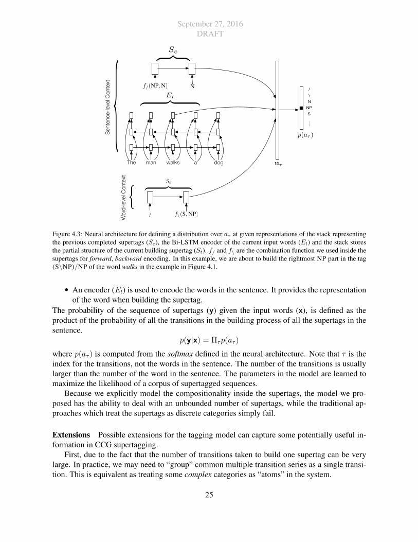
Model With the Tagging transition system, we can build a discriminative left-to-right taggerwith the neural architecture illustrated in Figure 4.3. We use Stack LSTMs (Dyer et al., 2015) tomodel the stack structures and Bi-directional LSTMs to model the encoder of the lexical inputs.Three components are used when computing the probability of a single tagging transition p(aτ ).• A stack (St) is the stack described in the transition system which is used to store partially

built structures within a supertag.• A (optional) stack (Sc) saves the history of completed CCG supertags built from the previ-

ous words in the sentence. After successfully built a supertag from St, the compositionalrepresentation of that tag will be pushed onto Sc.

24


Scz }| {

man walksThe a dog

/

Stz }| {

f/(NP, N) N

f\(S, NP)

NP

\/

N

S……

p(a⌧ )

u⌧

Elz }| {{S

ente

nce-leve

l Conte

xt

Word

-leve

l Conte

xt

{Figure 4.3: Neural architecture for defining a distribution over aτ at given representations of the stack representingthe previous completed supertags (Sc), the Bi-LSTM encoder of the current input words (El) and the stack storesthe partial structure of the current building supertag (St). f/ and f\ are the combination function we used inside thesupertags for forward, backward encoding. In this example, we are about to build the rightmost NP part in the tag(S\NP)/NP of the word walks in the example in Figure 4.1.

• An encoder (El) is used to encode the words in the sentence. It provides the representationof the word when building the supertag.

The probability of the sequence of supertags (y) given the input words (x), is defined as theproduct of the probability of all the transitions in the building process of all the supertags in thesentence.

p(y|x) = Πτp(aτ )

where p(aτ ) is computed from the softmax defined in the neural architecture. Note that τ is theindex for the transitions, not the words in the sentence. The number of the transitions is usuallylarger than the number of the word in the sentence. The parameters in the model are learned tomaximize the likelihood of a corpus of supertagged sequences.

Because we explicitly model the compositionality inside the supertags, the model we pro-posed has the ability to deal with an unbounded number of supertags, while the traditional ap-proaches which treat the supertags as discrete categories simply fail.

Extensions Possible extensions for the tagging model can capture some potentially useful in-formation in CCG supertagging.

First, due to the fact that the number of transitions taken to build one supertag can be verylarge. In practice, we may need to “group” common multiple transition series as a single transi-tion. This is equivalent as treating some complex categories as “atoms” in the system.

25


Second, it is known that modifiers are more likely to appear in the CCG supertag sequences(Garrette et al., 2015). For example, (S\NP)/(S/NP) is more likely than (S\NP)/(NP\NP).To model this effect, one possible solution is to add a new transition COPY which basicallycopies the completed category on the top of the stack and push it onto the stack. This createsa “short-cut” for the model to remember the previous generated categories since originally thiswill involve a series of transitions.

Third, tag combinability is an important attribute in CCG. Its implication is that partial su-pertag structures will often recur during the construction process. To capture this intuition, weplan to introduce a cache of built partial categories (and possible other categories by applying thecombination rules). Every time we predict a transition, we pull information from this cache usingthe attention mechanism (Xu et al., 2015a). This may help the model to build more combinabletags and avoiding invalid supertag sequences.

Another way to capture the tag combinability is to use a variant of the tagging transitionsystem which consider a pair of adjacent tags together. In this variant, we mainly have twoadditional classes of transitions.• RULE(R) where R ∈ {>,<,> B, < B, < B×} indicts which rule in Figure 4.2 is used

combine the two adjacent supertags (in practice, the oracle can be generated in a left-to-right greedy manner). Following this action, the system constructs two supertags us-ing the same transitions in the original tagging system but when a combinator or part ispre-determined by the applied rule, it simple uses the corresponding embedding withoutreconstructing them.

• NEW makes the system to construct a supertag as usual. This rule is used when we buildtags that can’t be combined with the previous one.

4.2.1 CCG Parsing Transition System

Bottom-up Transition System Zhang and Clark (2011) propose a bottom-up approach forCCG parsing. They introduce two classes of transitions operated between supertags1. The algo-rithm initializes the buffer with the supertag sequence of the sentence.• COMBINE(X) pops out the top two supertags on the stack, combines them using rule X

and pushes it back. X is one of the five operators combining the supertags (Figure 4.2).• SHIFT pops the current supertag on the buffer and push it on to the stack.With the existence of the previous tag history stack (Ec) in the tagging model, building a

joint-parsing and supertagging model is easy if we use the bottom-up CCG parsing transitions.The model just alternate between parsing and tagging transitions where the SHIFT action in theparsing transitions lets the tagging transition to construct a new supertag and push it to the stack2.

Top-down Transition System Hockenmaier and Steedman (2002) presents a generative modelof CCG derivations, based on various techniques from the statistical parsing literature (Collins,2003; Charniak, 1997; Goodman, 2000). Inspired by these work, we propose a novel transition

1In this section, we do not consider unary rules in the CCG, but extending them into the model is straight-forward.2The parsing process may fail during the decoding time but tagging accuracy is still evaluable in that case.

26


system that builds the tree in a top-down manner. It can condition on all the previously generatedstructure with the use of neural models.• CATEGORY(X ) introduces an “open CCG category” X on top of the stack.• REDUCE closes the open CCG category on the stack. It pops out its derivations from the

stack and pushes the category symbol back onto the stack.• RULE(R) where R ∈ {>,<,> B, < B, < B×} indicts which rule in Figure 4.2 should be

used to break down the category on top of the stack. It picks the Y category for the rule andthen pushes the first open category onto the stack. It has to wait until a “reduce” transitionfinishes the building of the first category and pushes the second category onto the stack.

With all these transition systems, the generative model for CCG supertagging and parsing canbe easily derived. The main difference is every time the model completely generates a supertag,it needs to generate the word associated with it from the tag embedding. Dyer et al. (2016)observe, as hypothesized in Henderson (2004), that larger, unstructured, conditioning contextsare harder to learn from, and provide opportunities to overfit. However, the generative modelwith access to relatively fewer information may perform better. We plan to use this frameworkin our work to see whether that improves the final performance.

4.3 ConclusionWe propose to model the compositionality both inside and between the CCG supertags. In theory,our model has the ability to handle an unbounded number of supertags where structurally naivemodels simply fail. Previous works also suggests that explicit modeling of such informationcan leads to better accuracy (Srikumar and Manning, 2014) and less supervision (Garrette et al.,2015).

27


28


Chapter 5

Conclusion

The work presented in this thesis describes several instances of how assumptions about struc-ture can be integrated naturally into neural representation learners for NLP problems, withoutsacrificing computational efficiency.

We stress the importance of explicitly representing structure in neural models. We argue that,when comparing with structurally naive models, models that reason about the internal linguisticstructure of the data demonstrate better generalization performance.

The techniques proposed in thesis automatically learn the structurally informed representa-tions of the inputs. These representations and components in the models can be better integratedwith other end-to-end deep learning systems within and beyond NLP (Cho et al., 2014; Graveset al., 2013, inter alia).

We propose to shed light on the interpretability of neural models by further investigation ofhow the model understands more complex things from composing the small parts and takingadvantage of the composition functions governed by linguistically sound assumptions on struc-tures.

29


30


Chapter 6

Timeline

The timeline for this thesis will be organized around paper submission deadlines, and the overallgoal is to complete this thesis within a year (defending in October 2017).• Winter 2016: Work on extending the model in §2, Target: ACL 2017.• Spring 2017: Work on modeling the compositionality in CCG supertagging in §4. Target:

EMNLP 2017.• Summer 2017: Write dissertation.• October 2017: Thesis defense.

31


32


Bibliography

Ossama Abdel-Hamid, Li Deng, Dong Yu, and Hui Jiang. Deep segmental neural networks forspeech recognition. In Proc. INTERSPEECH, pages 1849–1853, 2013. ??

Daniel Andor, Chris Alberti, David Weiss, Aliaksei Severyn, Alessandro Presta, KuzmanGanchev, Slav Petrov, and Michael Collins. Globally normalized transition-based neural net-works. Proc. ACL, 2016. 1

Dzmitry Bahdanau, Kyunghyun Cho, and Yoshua Bengio. Neural machine translation by jointlylearning to align and translate. In Proc. ICLR, 2015. 1

Daniel M Bikel. On the parameter space of generative lexicalized statistical parsing models.PhD thesis, University of Pennsylvania, 2004. 2.2

Xavier Carreras, Michael Collins, and Terry Koo. Tag, dynamic programming, and the percep-tron for efficient, feature-rich parsing. In Proceedings of the Twelfth Conference on Compu-tational Natural Language Learning, pages 9–16. Association for Computational Linguistics,2008. 2.2

Eugene Charniak. Statistical parsing with a context-free grammar and word statistics. AAAI/IAAI,2005(598-603):18, 1997. 4.2.1

Eugene Charniak. A maximum-entropy-inspired parser. In Proceedings of the 1st North Amer-ican chapter of the Association for Computational Linguistics conference, pages 132–139.Association for Computational Linguistics, 2000. 2.2

Eugene Charniak and Mark Johnson. Coarse-to-fine n-best parsing and maxent discriminativereranking. In Proceedings of the 43rd Annual Meeting on Association for ComputationalLinguistics, pages 173–180. Association for Computational Linguistics, 2005. 2, 2.2

Danqi Chen and Christopher D Manning. A fast and accurate dependency parser using neuralnetworks. In Proc. EMNLP, 2014. 1

Kyunghyun Cho, Bart van Merrienboer, Caglar Gulcehre, Fethi Bougares, Holger Schwenk, andYoshua Bengio. Learning phrase representations using RNN encoder-decoder for statisticalmachine translation. Pro. EMNLP, 2014. 5

Jan K Chorowski, Dzmitry Bahdanau, Dmitriy Serdyuk, Kyunghyun Cho, and Yoshua Bengio.Attention-based models for speech recognition. In Advances in Neural Information ProcessingSystems, pages 577–585, 2015. ??, ??

Michael Collins. Head-driven statistical models for natural language parsing. Computationallinguistics, 29(4):589–637, 2003. 2.3, 4.2.1

33


Michael Collins and Terry Koo. Discriminative reranking for natural language parsing. Compu-tational Linguistics, 31(1):25–70, 2005. 2.3

Michael Collins, Lance Ramshaw, Jan Hajic, and Christoph Tillmann. A statistical parser forczech. In Proceedings of the 37th annual meeting of the Association for Computational Lin-guistics on Computational Linguistics, pages 505–512. Association for Computational Lin-guistics, 1999. 2.2

Marie-Catherine De Marneffe and Christopher D Manning. The stanford typed dependenciesrepresentation. In Coling 2008: Proceedings of the workshop on Cross-Framework and Cross-Domain Parser Evaluation, pages 1–8. Association for Computational Linguistics, 2008. 2.5

Yuan Ding and Martha Palmer. Machine translation using probabilistic synchronous dependencyinsertion grammars. In Proceedings of the 43rd Annual Meeting on Association for Computa-tional Linguistics, pages 541–548. Association for Computational Linguistics, 2005. 2.3

John Duchi, Elad Hazan, and Yoram Singer. Adaptive subgradient methods for online learningand stochastic optimization. The Journal of Machine Learning Research, 12:2121–2159, 2011.2.2.2

Chris Dyer, Miguel Ballesteros, Wang Ling, Austin Matthews, and Noah A Smith. Transition-based dependency parsing with stack long short-term memory. In Proc. ACL, 2015. 1, 4.2

Chris Dyer, Adhiguna Kuncoro, Miguel Ballesteros, and Noah A Smith. Recurrent neural net-work grammars. Proc. NAACL, 2016. 1, 4.2.1

Jason Eisner and Giorgio Satta. Efficient parsing for bilexical context-free grammars and headautomaton grammars. In Proceedings of the 37th annual meeting of the Association for Com-putational Linguistics on Computational Linguistics, pages 457–464. Association for Compu-tational Linguistics, 1999. 2.1.1

Dan Garrette, Chris Dyer, Jason Baldridge, and Noah A Smith. Weakly-supervised grammar-informed bayesian ccg parser learning. In AAAI, pages 2246–2252, 2015. 1, 4, 4.2, 4.2, 4.3

Joshua Goodman. Probabilistic feature grammars. In Advances in Probabilistic and Other Pars-ing Technologies, pages 63–84. Springer, 2000. 4.2.1

Alex Graves. Hierarchical subsampling networks. In Supervised Sequence Labelling with Re-current Neural Networks, pages 109–131. Springer, 2012. 3.2, 3.4

Alex Graves and Navdeep Jaitly. Towards end-to-end speech recognition with recurrent neuralnetworks. In Proc. ICML, 2014. 3.1

Alex Graves and Jurgen Schmidhuber. Framewise phoneme classification with bidirectionalLSTM and other neural network architectures. Neural Networks, 18(5):602–610, 2005. 3.1

Alex Graves, Santiago Fernandez, Faustino Gomez, and Jurgen Schmidhuber. Connectionisttemporal classification: labelling unsegmented sequence data with recurrent neural networks.In Proc. ICML, 2006a. 1

Alex Graves, Santiago Fernandez, Faustino Gomez, and Jurgen Schmidhuber. Connectionisttemporal classification: Labelling unsegmented sequence data with recurrent neural networks.In Proc. ICML, 2006b. 1, 2, 3.5.1

34


Alex Graves, A-R Mohamed, and Geoffrey Hinton. Speech recognition with deep recurrentneural networks. In Proc. ICASSP, pages 6645–6649. IEEE, 2013. 1, ??, ??, 5

David Hall, Greg Durrett, and Dan Klein. Less grammar, more features. In ACL, 2014. 2.2.1

Yanzhang He and Eric Fosler-Lussier. Efficient segmental conditional random fields for phonerecognition. In Proc. INTERSPEECH, pages 1898–1901, 2012. ??

James Henderson. Discriminative training of a neural network statistical parser. In Proceedingsof the 42nd Annual Meeting on Association for Computational Linguistics, page 95. Associa-tion for Computational Linguistics, 2004. 4.2.1

Sepp Hochreiter and Jurgen Schmidhuber. Long short-term memory. Neural computation, 9(8):1735–1780, 1997. 3.1

Julia Hockenmaier and Mark Steedman. Generative models for statistical parsing with combi-natory categorial grammar. In Proceedings of the 40th Annual Meeting on Association forComputational Linguistics, pages 335–342. Association for Computational Linguistics, 2002.4.2.1

Julia Hockenmaier and Mark Steedman. Ccgbank: a corpus of ccg derivations and dependencystructures extracted from the penn treebank. Computational Linguistics, 33(3):355–396, 2007.4.1

Andrej Karpathy and Li Fei-Fei. Deep visual-semantic alignments for generating image descrip-tions. In Proc. CVPR, 2015. 3.1

Robert H. Kassel. A comparison of approaches to on-line handwritten character recognition.PhD thesis, Massachusetts Institute of Technology, 1995. 3.5.1

Diederik Kingma and Jimmy Ba. Adam: A method for stochastic optimization. arXiv preprintarXiv:1412.6980, 2014. 3.5.1

Dan Klein and Christopher D Manning. Accurate unlexicalized parsing. In Proceedings of the41st Annual Meeting on Association for Computational Linguistics-Volume 1, pages 423–430.Association for Computational Linguistics, 2003. 2.1.3, 2.2

Lingpeng Kong, Chris Dyer, and Noah A Smith. Segmental recurrent neural networks. Proc.ICLR, 2015a. 1, 3

Lingpeng Kong, Alexander M Rush, and Noah A Smith. Transforming dependencies into phrasestructures. In Proc. NAACL, 2015b. 1, 2

Kenton Lee, Mike Lewis, and Luke Zettlemoyer. Global neural ccg parsing with optimalityguarantees. arXiv preprint arXiv:1607.01432, 2016. 1, 4

Mike Lewis and Mark Steedman. A* ccg parsing with a supertag-factored model. In EMNLP,pages 990–1000, 2014a. 1, 4

Mike Lewis and Mark Steedman. Improved ccg parsing with semi-supervised supertagging.Transactions of the Association for Computational Linguistics, 2:327–338, 2014b. 1, 4

Liang Lu, Lingpeng Kong, Chris Dyer, Noah A Smith, and Steve Renals. Segmental recurrentneural networks for end-to-end speech recognition. Proc. Interspeech, 2016. 1, 3

Christopher D Manning. Computational linguistics and deep learning. Computational Linguis-

35


tics, 2016. 1

Mitchell P Marcus, Mary Ann Marcinkiewicz, and Beatrice Santorini. Building a large annotatedcorpus of english: The penn treebank. Computational linguistics, 19(2):313–330, 1993. 1, 2.3,4

Andre FT Martins, Miguel Almeida, and Noah A Smith. Turning on the turbo: Fast third-ordernon-projective turbo parsers. In ACL (2), pages 617–622, 2013. 2.3, 2.4

Ryan McDonald. Discriminative learning and spanning tree algorithms for dependency parsing.PhD thesis, University of Pennsylvania, 2006. 2.2.1

Tom M Mitchell. The need for biases in learning generalizations. Department of ComputerScience, Laboratory for Computer Science Research, Rutgers Univ. New Jersey, 1980. 1

Joakim Nivre. Algorithms for deterministic incremental dependency parsing. ComputationalLinguistics, 34(4):513–553, 2008. 4.2

Joakim Nivre, Johan Hall, and Jens Nilsson. Maltparser: A data-driven parser-generator fordependency parsing. In Proceedings of LREC, volume 6, pages 2216–2219, 2006. 2.4

Slav Petrov and Dan Klein. Improved inference for unlexicalized parsing. In HLT-NAACL, pages404–411. Citeseer, 2007. 2, 2.2

Lawrence R. Rabiner. A tutorion on hidden Markov models and selected applications in speechrecognition. Proc. IEEE, 77(2), 1989. 2

Sunita Sarawagi and William W. Cohen. Semi-Markov conditional random fields for informationextraction. In Proc. NIPS, 2004. 3.3

Richard Socher, John Bauer, Christopher D Manning, and Andrew Y Ng. Parsing with compo-sitional vector grammars. In Proc. ACL, pages 455–465, 2013. 2.2

Vivek Srikumar and Christopher D Manning. Learning distributed representations for structuredoutput prediction. In Advances in Neural Information Processing Systems, pages 3266–3274,2014. 1, 4, 4.3

Mark Steedman. The syntactic process, volume 24. MIT Press, 2000. 1

Hao Tang, Weiran Wang, Kevin Gimpel, and Karen Livescu. Discriminative segmental cascadesfor feature-rich phone recognition. In Proc. ASRU, 2015. ??, 3.5.2

Ben Taskar, Carlos Guestrin, and Daphne Koller. Max-margin Markov networks. In Advancesin Neural Information Processing Systems 16, 2004a. 2.2.2

Ben Taskar, Carlos Guestrin, and Daphne Koller. Max-margin Markov networks. NIPS, 16:25,2004b. 3.5.1

Fei Xia and Martha Palmer. Converting dependency structures to phrase structures. In Proceed-ings of the first international conference on Human language technology research, pages 1–5.Association for Computational Linguistics, 2001. 2

Fei Xia, Owen Rambow, Rajesh Bhatt, Martha Palmer, and Dipti Misra Sharma. Towards a multi-representational treebank. In The 7th International Workshop on Treebanks and LinguisticTheories. Groningen, Netherlands, 2009. 2

Kelvin Xu, Jimmy Ba, Ryan Kiros, Kyunghyun Cho, Aaron Courville, Ruslan Salakhutdinov,

36


Richard S Zemel, and Yoshua Bengio. Show, attend and tell: Neural image caption generationwith visual attention. arXiv preprint arXiv:1502.03044, 2015a. 4.2

Wenduan Xu, Michael Auli, and Stephen Clark. Ccg supertagging with a recurrent neural net-work. In Proceedings of the 53rd Annual Meeting of the Association for Computational Lin-guistics and the 7th International Joint Conference on Natural Language Processing, vol-ume 2, pages 250–255, 2015b. 1, 4

Naiwen Xue, Fei Xia, Fu-Dong Chiou, and Martha Palmer. The Penn Chinese TreeBank: Phrasestructure annotation of a large corpus. Natural Language Engineering, 11(2):207–238, 2005.2.3

Yuan Zhang and David Weiss. Stack-propagation: Improved representation learning for syntax.arXiv preprint arXiv:1603.06598, 2016. 2.5

Yue Zhang and Stephen Clark. Shift-reduce ccg parsing. In Proceedings of the 49th AnnualMeeting of the Association for Computational Linguistics: Human Language Technologies-Volume 1, pages 683–692. Association for Computational Linguistics, 2011. 4.2.1

Muhua Zhu, Yue Zhang, Wenliang Chen, Min Zhang, and Jingbo Zhu. Fast and accurate shift-reduce constituent parsing. In ACL (1), pages 434–443, 2013. 2.3, 2.2, 2.4

Geoffrey Zweig. Classification and recognition with direct segment models. In Proc. ICASSP,pages 4161–4164. IEEE, 2012. ??

37

Neural Representation Learning in Linguistic Structured ...

Documents