Oligotrophication of Lake Tegel and Schlachtensee, Berlin · Oligotrophication of Lake Tegel and Schlachtensee, Berlin . Analysis of system components, causalities and response thresholds

Oligotrophication of Lake Tegel and Schlachtensee, Berlin Analysis of system components, causalities and response thresholds compared to responses of other waterbodies

TEXTE

45/2011

Oligotrophication of Lake Tegel and Schlachtensee, Berlin

Analysis of system components, causalities and response thresholds compared to responses of other waterbodies

by

Dr. Ingrid Chorus Inke Schauser

Umweltbundesamt

and guest authors

UMWELTBUNDESAMT

| TEXTE | 45/2011

This publication is only available online. It can be downloaded from http://www.uba.de/uba-info-medien-e/4144.html.

The comprehensive scientific evaluation presented in this booklet was developed in the project OLIGO, funded by Veolia Water and Berliner Wasserbetriebe through the Kompetenzzentrum Wasser Berlin.

ISSN 1862-4804

Study performed by: Federal Environment Agency (Umweltbundesamt) Wörlitzer Platz 1

06844 Dessau-Roßlau (Germany)

Study completed in: June 2011

Publisher: Federal Environment Agency (Umweltbundesamt) Wörlitzer Platz 1 06844 Dessau-Roßlau Germany Phone: +49-340-2103-0 Fax: +49-340-2103-0 Email: [email protected] Internet: http://www.umweltbundesamt.de

http://fuer-mensch-und-umwelt.de/

Edited by: Section II 3 Drinking and Swimming Pool Water Hygiene Dr. Ingrid Chorus, Inke Schauser

Dessau-Roßlau, July 2011

http://www.uba.de/uba-info-medien-e/4144.html�

http://www.umweltbundesamt.de/�

http://fuer-mensch-und-umwelt.de/�

I

Abstract (English) Lake Tegel and Schlachtensee in Berlin show a uniquely pronounced trophic recovery in response to an abrupt and drastic (40- to 100-fold) reduction of their external phosphorus (P) load through P-stripping at their main inflow which exchanges the lake water volume about 5 times per year for Lake Tegel and about 1.5 times for Schlachtensee. In response, annual mean concentrations of total phosphorus (TP) declined exponentially from 600-800 µg L-1 before restoration to meanwhile 30 µg L-1 in Lake Tegel and 18 µg L-1 in Schlachtensee. Phytoplankton biomass started responding only after TP concentrations had declined to less than 100 µg L-1, and TP clearly determines biomass levels only below a TP threshold of ~50 µg L-1. Below this, annual mean concentrations of chlorophyll-a (as quantitative measure for phytoplankton biomass) declined from previously 40-60 µg L-1 to meanwhile 6-11 µg L-1.

OLIGO conducted a comprehensive analysis of lake recovery data available for 20 years for Lake Tegel and 25 years from Schlachtensee. Targets were to elucidate causal relationships, i.e. the mechanisms and processes of lake recovery, to develop lake specific numerical models that support management and to discern non-continuous or threshold patterns of restoration response, as such switches may generally be crucial for successful lake therapy. OLIGO further compared these results to data gleaned from many other lake and reservoir data. Key results are the following:

The lake-specific numerical models developed in OLIGO clarified

for Lake Tegel that

:

1. the main remaining phosphorus (P) source is inflow of P-rich water from the River Havel. The most important management target therefore is to keep as much pf the P-rich River Havel water out of the lake as possible by maintaining a minimum throughflow of low-P water from the phosphorus stripping plant of 2.5 m³ per second as annual mean and by optimising time patterns of throughflow to maximise summer throughflow at the expense of that in winter;

2. on an annual basis the sediments functioned as a sink for P in most years, but they remain a relevant short-term seasonal source of P. P from the lake’s sediments largely originates from the mineralisation of recently sedimented material. Therefore it is likely to decline rapidly in response to external load reduction, but it can increase if hypolimnion temperatures increase, e.g. through (artificial) mixing. Redox-sensitive adsorption to iron proved to play a subordinate role which can be enhanced by using iron as preferred flocculant for P stripping at the inflow;

3. an increase of storm frequency would increase P concentrations.

for Schlachtensee that

4. redox sensitive P desorption from the sediments is the more relevant remaining source for the accumulation of P in the water layers above the sediments. However, this process has less impact on trophic state of the lake than in Lake Tegel, because throughout the summer very stable thermal stratification largely keeps the desorbed P in the deep layers where it is poorly accessible for phytoplankton growth;

II

5. a 1.5 – 3-fold increase of throughflow of low-P water (as is currently under planning) would reduce in-lake TP-concentrations from from currently 20-25 µg L-1 to 12-15 µg L-1 i.e. scarcely more than the P-stripping plant discharge concentrations of ~8 µg L-1.

For both lakes the lake-specific numerical models showed the impact of internal measures (aeration in Lake Tegel and hypolimnion withdrawal from Schlachtensee) to be minor in relation to the pronounced external load reduction. To maintain their current trophic status, phosporus stripping at their main inflow will continue to be necessary until the River Havel reaches TP-concentrations similar to those of the lakes.

Phytoplankton biomass responses to declining TP concentrations

6. Resource use efficiencies of the phytoplankton, expressed as the ratio of the concen-trations of chlorophyll-a to TP, were maximal at low or intermediate levels of TP;

commonly show some non-linearity but can nonetheless be roughly predicted from TP concentrations:

7. Only 7 of the 19 lakes analysed showed TP thresholds for the response of phytoplankton biomass – at concentrations influenced by the depth of the epilimnion. For the majority of these lakes, no TP threshold became evident, in part because TP-reductions were not sufficiently pronounced and/or because other factors, particularly biotic interactions, exerted a stronger impact;

8. The extremely pronounced TP-threshold of ~50 µg L-1 for Lake Tegel as well as for Schlachtensee is explicable by a switch from light to P imitation and by resilience of dominance of cyanobacterial species;

9. In spite of some non-linear restoration response patterns the Vollenweider regression remains a useful tool for predicting the response of phytoplankton biomass to the reduction of TP-concentrations, though with a wide range of uncertainty. Reducing this uncertainty requires including prediction of shifts in the biota;

10. A closer prediction of phytoplankton biomass (in terms of chlorophyll-a-concen-trations) is possible for Lake Tegel by including not only TP but also daily global irradiation (fit of r = 0.71 for 1986-2004). This did not apply to Schlachtensee, where hydrophysical conditions and zooplankton grazing have more impact on phyto-plankton growth and loss rates. There, even the more complex model PROTECH proved only partially successful: it did not perform well in predicting biomass and major taxonomic groups for early spring at low light intensity and temperature.

The response of phytoplankton species composition to restoration

11. for Cyanobacteria a very clear TP-dependency of biomass and dominance: in the two Berlin lakes they became subdominant (biovolume <3 mm³ L-1) or insignificant once summer TP concentration remained below 25 µg L-1. The statistical results from 3000

was analysed in detail for the two Berlin lakes, supplemented by a statistical model begun in earlier projects and further elaborated by OLIGO: Using the data of 1500-3000 samples from 20-210 water-bodies this model describes the habitats of 18 common phytoplankton taxa in relation to 8 variables that impact on growth and capacity for biomass, thus allowing an assessment of their likelihood to occur under a given condition. Key results include

III

samples and 210 water-bodies show that cyanobacterial biovolumes of >0.1 mm³ L-1 are highly unlikely in meso- or oligotrophic water-bodies at TP <25 µg L-1;

12. for Chrysophyta also a very clear – though indirect – TP-dependency of occurrence: in the two Berlin lakes they were absent during the hypertrophic phases, during which high rates of photosynthesis caused summer pH of 8.5 – 9.5. They appeared once pH remained <8.7 due to lower overall phytoplankton biomass levels and thus lower rates of photosynthesis.;

13. for the diatoms a slight shift from Diatoma spp. and Fragilaria spp. in eutrophic water-bodies to Asterionella formosa under less eutrophic conditions;

14. for the two Dinophyte taxa analysed statistically, Ceratium spp. and Peridinium spp., an enhanced likelihood to attain significant populations under mesotrophic conditions, although the impact of stratification on their occurrence was more relevant than that of TP concentrations;

15. for most other taxa less clear restoration responses – some formed sizable popula-tions only for a few years in sequence. This indicates the relevance of the “phyto-plankton memory” of a lake, i.e. inocula of taxa which attained substantial biomass seeding next year’s population. For Lake Tegel’s short period of re-eutrophication (i.e. increased TP-levels from 1998-2001), this mechanism probably buffered a corre-sponding increase of phyoplankton biomass and a return of cyanobacterial blooms.

Gross primary production, determined as oxygen production through photosynthesis during a few years (including years with a pronounced oligotrophication response of phytoplankton only for Schlachtensee) shows

16. a close relationship of depth-integrated rates (i.e. per m² of lake surface) both to euphotic phytoplankton biomass concentratins and to global irradiation, confirming that gross primary production integrals can be predicted from data for these key variables;

17. a very pronounced reduction of maximal rates per m³ in response to reduced biomass densities, but a substantially increased depth of the euphotic zone, resulting in a reduction of depth-integrated rates only by about 25% by the late 1980s;

18. a more rapid recovery of Schlachtensee’s oxygen budget than would be expected from depth-integrated gross primary production: the duration and spatial extention of oxygen depletion decreased shortly after phytoplankton densities had dropped, even though gross primary production integrals were still high. This suggests that mineralisation processes depend not only on the absolute amount of carbon fixed per m² of a lake’s surface, but also on its spatial distribution.

The trophic recovery process has cascaded from reduced TP-concentrations down the trophic levels in both Berlin Lakes. In Schlachtensee, it has progressed farther towards a new equilibrium than in Lake Tegel, which still has higher levels of TP and phytoplankton. Much of Schlachtensee ‘s lake bottom is now covered by aquatic macrophytes, and the reed belt is re-growing. Protecting the shorelines and their vegetation belts from damage through erosion and wave action is important for both lakes in order to stabilise the aquatic macrophytes, as these bind P and thus exert positive feed back on the lakes’ P budgets.

IV

General lessons for trophic recovery are that

19. while generic models such as the Vollenweider regressions do allow useful rough predictions of restoration responses, the uncertainty of their results is necessarily substantial due to the individually specific combinations of conditions in a given waterbody. Lake-specific numerical models (provided sufficient data are available) proved to be powerful tools for more detailed analysis and differentiated predictions of responses to management measures;

20. where the speed of trophic recovery in response to external load reduction is uncertain, it is worthwhile to allow for some years of observation before implementing supporting internal measures, particularly if TP-concentrations are declining without phytoplankton (yet) declining correspondingly;

21. public communication should include such uncertainties of the time horizon for visible improvement to avoid disappointment and undue pressure for further action;

22. in highly eutrophic urban and peri-urban settings reducing the external P-load sufficiently to control phytoplankton biomass and cyanobacterial blooms may be a managerial and technical challenge. The success at Lake Tegel and Schlachtensee shows that effective technology is available to tackle this challenge, but this may require some investment and sustained long-term operation of the technology.

Key questions for future restoration research include

i. an in-depth analyses of the now available longer-term data series of restoration responses across the globe in order to identify generic response patterns more clearly, particularly of thresholds of P limitation, of biotic interactions that cause resilience, and of TP levels that can crack such resilience;

ii. further development of the statistical phytoplankton model with a broader data base and interlinking of the growth conditions in order to make it a prognostic tool;

iii. testing the hypothesis that a key cause for resilience to trophic change is the determination of next year’s phytoplankton populations by overwintering inocula;

iv. specifically for the Berlin Lakes the determination of phosphorus loads from precipi-tation, because as other external loads decline the contribution of precipitation to the P budget is increasingly important.

V

Abstract (German) Der Tegeler See und der Schlachtensee in Berlin zeigten eine einmalig stark ausgeprägte Verbesserung ihres trophischen Zustandes in Reaktion auf eine abrupte und drastische Reduktion der externen Zufuhr an Phosphor (P) durch P-Elimination im Hauptzufluss, der das Wasservolumen des Tegeler Sees rechnerisch 5-mal pro Jahr und das des Schlachtensees 1,5-mal pro Jahr austauscht. Dadurch gingen die Konzentrationen an Gesamtphosphor (TP) exponentiell zurück – im Jahresmittel von 600-800 µg L-1 vor der Sanierung auf mittlerweile 30 und 18 µg L-1. Die Phytoplanktonbiomasse begann erst zu reagieren, als die TP-Konzentrationen 100 µg L-1 unterschritten hatten, und sie zeigt eine eindeutige TP-Abhängigkeit erst unterhalb einer TP Schwellenkonzentration von ~50 µg L-1. Darunter ging die Chlorophyll-a-Konzentration (als quantitatives Maß der Phytoplankton-biomasse) zurück – im Jahresmittel von ehemals 40-60 µg L-1 auf nunmehr 6-11 µg L-1.

OLIGO führte eine umfassende Analyse der Datenreihen zu diesem Erholungsprozess, die für den Tegeler See 20 und für den Schlachtensee 25 Jahre umfassen. Ziele waren die Klärung kausaler Zusammenhänge, d.h. der Mechanismen und Prozesse dieser Erholung, und die Entwicklung von Gewässer-spezifischen numerischen Modellen zur Unterstützung ihrer Bewirtschaftung sowie das Erkennen nicht-linearer Reaktionsmuster, insb. solcher mit einer Wirkschwelle, da solche „Schaltstellen“ für Sanierungsmaßnahmen erfolgskritisch sein können. Ferner hat OLIGO diese Ergebnisse mit Daten aus zahlreichen anderen Seen und Talsperren abgeglichen. Im Ergebnis stehen folgende Erkenntnisse:

Die in OLIGO entwickelten Seen-spezifischen Modelle klärten:

für den Tegeler See dass 1. die wesentliche verbleibende P-Quelle ist der Zufluss an P-reichem Havelwasser.

Das wichtigste Bewirtschaftungsziel ist daher, seinem Zustrom durch einen Mindestzufluss an P-armem Wasser aus der Eliminierungsanlage zu begegnen – im Jahresmittel sollte er nicht unter 2,5 m³ pro Sekunde liegen, bei Optimierung der jahreszeitlichen Verteilung durch höheren Zufluss im Sommer auf Kosten des Zuflusses im Winter;

2. im Jahresmittel fungiert das Sediment in den meisten Jahren als P-Falle, aber sie sind weiterhin eine relevante kurzzeitige saisonale P-Quelle. P aus dem Sediment stammt vorwiegend aus der Mineralisation von erst kürzlich sedimentiertem organischen Material. Daher reagiert sie wahrscheinlich rasch auf eine Reduktion der externen P-Fracht, kann aber durch höhere Temperaturen ansteigen, z.B. infolge von (künstlicher) Durchmischung. Die Bedeutung der redox-sensitiven Adsorption an Eisen erwies sich als nachranging. Allerdings kann diese gefördert werden, indem die Aufbereitungsanlage Eisen als bevorzugtes Fällmittel einsetzt;

3. eine Erhöhung der Häufigkeit von Stürmen würde die P-Konzentrationen erhöhen.

für den Schlachtensee dass 4. die redox-sensitive P-Desorption von den Sedimenten die wichtigere verbleibende

Quelle der P-Akkumulation in der Wasserschicht über dem Sediment ist. Allerdings

VI

hat dieser Prozess weniger Einfluss auf den trophischen Zustand als im Tegeler See da infolge der sehr stabilen thermischen Schichtung der desorbierte Phosphor während des Sommers weitgehend in tiefen Schichten verbleibt, so dass er für Phytoplanktonwachstum kaum verfügbar wird;

5. eine 1,5 – 3-fache Erhöhung der Durchströmung mit P-armem Wasser (wie derzeit geplant) würde die TP-Konzentrationen im See von derzeit 20-25 µg L-1 auf 12-15 µg L-1 reduzieren – damit lägen sie kaum über den ~8 µg L-1 im Ablauf der Eliminierungs-anlage.

Für beide Seen zeigten die numerischen Modelle, dass der Einfluss der internen Restaurierungsmaßnahmen (Belüftung im Tegeler See und Hypolimnion-Entzug im Schlachtensee) gering war in Relation zu der ausgeprägten Reduktion der externen P-Fracht. Um den derzeitigen trophischen Zustand beider Seen zu erhalten, wird die P-Elimination an ihren Zuflüssen solange weiterhin erforderlich bleiben, bis die TP-Konzen-tration der Havel ähnlich niedrige Werte erreicht hat.

Die Reaktion der Phytoplankton-Biomasse auf abnehmende TP-Konzentrationen ist häufig nicht linear, aber dennoch anhand der TP-Konzentrationen ungefähr prognostizierbar:

6. Die Ressourceneffizienz des Phytoplanktons, ausgedrückt als Relation der Konzen-trationen von Chlorophyll-a zu TP, war am höchsten bei geringen oder intermediären TP-Konzentrationen;

7. Eine TP-Schwelle für die Reaktion der Phytoplankton-Biomasse zeigten nur 7 der 19 untersuchten Gewässer, wobei die TP-Schwellenkonzentration von der Mächtigkeit des Epilimnions beeinflusst ist. In der Mehrzahl der Gewässer war keine TP-Schwelle erkennbar, z. T. aufgrund eines noch zu geringen TP-Rückgangs und/oder durch einen stärkeren Einfluss anderer Faktoren, insb. biotischer Interaktionen.

8. Die extrem stark ausgeprägte TP-Schwelle von ~50 µg L-1 für den Tegeler See und den Schlachtensee kann durch ein „Umschalten“ von Lichtlimitation auf P-Limitation erklärt werden; hinzu kam ein Beharrungsvermögen dominanter Cyanobakterienarten („resilience“);

9. Trotz mancher nicht-linearen Reaktionsmuster bleibt die Vollenweider Regression ein wertvolles Prognoseinstrument für die Reaktion der Phytoplankton-Biomasse auf die Reduktion der TP-Konzentration, wenngleich mit einer ausgeprägten Unsicherheits-marge. Diese zu reduzieren erfordert die Einbeziehung von Artenverschiebungen;

10. Eine engere Prognose der Phytoplankton-Biomasse (als Chlorophyll-a-Konzen-tration) ist für den Tegeler See möglich, indem nicht nur TP sondern auch die Globalstrahlung zugrunde gelegt wird (dies erreicht ein Fit von r = 0,71 für 1986-2004). Für den Schlachtensee trifft dies nicht zu, da hydrophysikalische Bedingungen und Fraßverluste durch Zooplankton einen stärkeren Einfluss auf die Wachstums- und Verlustraten des Phytoplanktons ausüben. Für diesen See erwies sich auch das komplexere Modell PROTECH nur teilweise als erfolgreich – für das frühe Frühjahr bei geringer Lichtintensität und Temperatur konnte es Biomasse und Hauptgruppen im Phytoplankton nicht prognostizieren.

VII

Die Reaktion der Artenzusammensetzung des Phytoplanktons auf die Restaurierung wurde im Detail für die 2 Berliner Seen analysiert, ergänzt durch ein statistisches Modell, dessen Entwicklung im Rahmen früherer Projekte begonnen und in OLIGO weitergeführt wurde: Auf der Grundlage von Daten von 1500-3000 Proben aus 20-210 Gewässern beschreibt dieses Modell die Habitate von 18 häufigen Phytoplanktonarten in Relation zu 8 Variablen, von denen Wachstumsraten und die Kapazität für Biomasse abhängen. Somit ermöglicht es eine Bewertung ihrer Auftrittswahrscheinlchkeit unter einer gegebenen Bedingung. Zu den wesentlichen Ergebnissen zählen

11. für die Cyanobakterien eine sehr deutliche TP-Abhängigkeit ihrer Biomasse und Dominanz: in den zwei Berliner Seen wurden sie subdominant (Biovolumen <3 mm³ L-1) oder unbedeutend als die TP-Konzentrationen im Sommer unterhalb von 25 µg L-1 blieben. Die statistischen Ergebnisse aus 3000 Proben und 210 Gewässern zeigen, dass Cyanobakterienbiovolumina >0,1 mm³ L-1 in meso- oder oligotrophen Gewässern mit TP <25 µg L-1 äußerst unwahrscheinlich sind;

12. für die Chrysophyceen ebenfalls eine sehr deutliche indirekte TP-Abhängigkeit ihres Vorkommens: in den zwei Berliner Seen fehlten sie während ihrer hypertrophen Phase, während der hohe Photosyntheseraten zu pH-Werten von 8,5-9,5 führten;

13. für die Diatomeen eine gering ausgeprägte Verschiebung von Diatoma spp. und Fragilaria spp. in eutrophen Gewässern zu Asterionella formosa unter weniger eutrophen Bedingungen;

14. für die zwei statistisch analysierten Dinophyta, Ceratium spp. und Peridinium spp., eine erhöhte Wahrscheinlichkeit für größere Populationen unter mesotrophen Bedingungen, wobei die Schichtungsstabilität für ihr Vorkommen noch relevanter war als die TP-Konzentration;

15. für die meisten anderen Arten eine weniger deutliche Reaktionen auf die Restaurierung – manche bildeten nur in einigen aufeinanderfolgenden Jahren quantifizierbare Populationen aus. Dies weist auf die Bedeutung des „Phytoplankton Gedächtnisses“ eines Gewässers, d.h. Inocula von Taxa mit substantieller Biomasse als Grundlage für das Populationswachstum im Folgejahr. Für die kurze Phase der Re-Eutrophierung des Tegeler Sees (d.h. wieder ansteigende TP-Konzentrationen von 1998-2001) hat dieser Mechanismus wahrscheinlich einen entsprechenden Anstieg der Phytoplankton-Biomasse und insb. die Rückkehr der Cyanobakterien-blüten abgepuffert.

Die Brutto-Primärproduktion

16. einen engen Zusammenhang der tiefenintegrierten Raten (d.h. pro m² Seeober-fläche) sowohl zu den Biomassekonzentrationen in der euphotischen Tiefe als auch zur Globalstrahlung, der bestätigt, dass Primärproduktionsintegrale gut aus Daten zu diesen zwei Schlüsselvariablen prognostiziert werden können;

, während einiger Jahre als Sauerstoffproduktion durch die Photosynthese gemessen (nur für den Schlachtensee einschließlich einiger Jahre mit ausgeprägter Oligotrophierungsreaktion des Phytoplanktons) zeigt

17. einen sehr ausgeprägten Rückgang der maximalen Raten pro m³ in Reaktion auf die geringere Biomassedichte, jedoch eine erhebliche Zunahme der Tiefe der

VIII

euphotischen Zone, mit dem Ergebnis eines Rückgangs der tiefeninegrierten Raten um nur etwa 25% bis Ende der 1980er Jahre;

18. eine deutlich raschere Erhohlung der Sauerstoffbilanz des Schlachtensees als aufgrund der Tiefenintegrale der Bruttoprimärproduktion erwartet: Die zeitliche und räumliche Ausdehnung von Sauerstoffmangel ging schon kurz nach dem Rückgang der Phytoplanktonbiomassedichte zurück, als Primärproduktionsintegrale noch hoch waren. Dies weist darauf hin, dass Mineralisationsprozesse nicht nur von der absoluten Menge des pro m² Seeoberfläche fixierten Kohlenstoffs abhängen, sondern auch von ihrer räumlichen Verteilung.

Der trophische Erholungsprozess ist in beiden Berliner Seen kaskadenartig von den reduzierten TP-Konzentrationen durch alle Trophie-Ebenen verlaufen. Im Schlachtensee ist er dichter an einem neuen Gleichgewicht angekommen als im Tegeler See, der noch auf einem höheren TP- und Phytoplanktonniveau liegt. Große Bereiche der Schlachtensee-Sedimente sind nunmehr mit aquatischen Makrophyten bedeckt, und der Schilfgürtel nimmt zu. Der Schutz der Ufer und seiner Pflanzengürtel vor Zerstörung durch Erosion und Wellen ist für beide Seen zur Stabilisierung der aquatischen Vegetation wichtig, denn diese bindet Phosphor und üben somit eine für die P-Budgets der Seen günstige Rückwirkung aus.

Allgemeine Lehren für die trophische Erholung

19. generische Modelle wie die Vollenweider Regressionen durchaus nützliche grobe Prognosen der Reaktion auf Restaurierung ermöglichen, die Ungewissheiten ihrer Ergebnisse jedoch notwendigerweise erheblich sind – infolge der individuell spezifischen Kombinationen von Bedingungen in einem Gewässer. Seen-spezifische numerische Modelle erweisen sich (sofern eine ausreichende Datenbasis vorhanden ist) als sehr aussagekräftige Werkzeuge für eine detailliertere Analyse und differenziertere Prognose der Reaktion auf Bewirtschaftungsmaßnahmen;

sind dass

20. wenn unklar ist, wie rasch ein Gewässer auf die Reduktion der externen P-Fracht reagiert, es sich lohnt, einige Jahre abwartend zu beobachten, bevor interne Sanierungsmaßnahmen ergriffen werden, insbesondere wenn die TP-Konzen-trationen weiterhin zurückgehen und das Phytoplankton (noch) keine entsprechende Reaktion zeigt;

21. die Öffentlichkeitsarbeit von Anbeginn die Ungewissheit über den Zeithorizont der Gewässerreaktion beinhalten sollte, um Endtäuschungen und unangebrachten Druck für weitere Maßnahmen zu vermeiden;

22. für stark eutrophierte urbane und peri-urbane Gewässer die ausreichende Reduktion der externen P-Fracht, um die Phytoplankton-Biomasse und Cyanobakterien-Massenentwicklungen wirksam einzudämmen, eine große Herausforderung ist – technisch wie auch für die Gewässerbewirtschaftung. Der Erfolg am Tegeler See und am Schlachtensee verdeutlicht, dass hierfür wirksame Techniken verfügbar sind, dass diese aber einige Investitionen in Anlagen und die nachhaltige Sicherung ihres längerfristigen Betriebs erfordern.

IX

Schlüsselfragen für künftige Restaurierungsforschung

i. eine vertiefte Analyse der inzwischen aus verschiedenen Erdteilen vorhandenen längeren Datenreihen zur Reaktion auf Restaurierung, um verallgemeinerbare Muster klarer herauszuarbeiten, insb. zu Schwellenwerten der P-Limitierung, zu reaktionsverzögernden biotischen Interaktionen sowie zu TP-Konzentrationen, mit denen solche Systemwiderstände durchbrochen werden können;

umfassen

ii. eine Weiterentwicklung des statistischen Phytoplankton-Modells zu einem Prognosewerkzeug mit einer breiteren Datenbasis und durch Verknüpfung von Wachstumsbedingungen;

iii. die Prüfung der Hypothese, dass überwinternde Inocula die Phytoplankton-populationen des Folgejahres prägen und somit einen wesentlichen Mechanismus für Systemwiderstände gegen trophische Veränderung darstellen;

iv. spezifisch für die Berliner Seen die Ermittlung der Phosphorfrachten durch Niederschlag, da deren relative Bedeutung im Zuge des Rückgangs anderer externer Frachten steigt.

X

Foreword and Acknowledgements for 25 years of Restoration Research

Lake Recovery in response to restoration may take decades – even after extremely pronounced load reduction, and ensuring long-term funding to study the response all the way to a new equilibrium is a challenge. For two Berlin lakes, Schlachtensee and Lake Tegel, restoration began in autumn of 1981 and 1985, respectively, with the operation of phosphorus elimination plants (PEPs) at the lakes’ inflows. Their construction was financed by the Berlin government, and they are operated (and meanwhile owned) by the Utility Berlin Water (“Berliner Wasserbetriebe”; BWB). For scientific supervision and for monitoring the lakes’ responses, during the 1980s and part of the 1990s the Berlin State Government provided funding to the Institute for Water, Soil and Air Hygiene (meanwhile part of the Federal Environment Agency – ”Umweltbundesamt”, UBA), and since then basic monitoring of Lake Tegel is performed by the city government’s laboratory. More detailed monthly sampling and analysis of both lakes was upheld at UBA by dedicated technicians – particularly Hans-Ulrich Wolf, Elke Pawlitzky, Katrina Laskus, Christa Kopplin and Ingrid Klinkmüller. The data thus generated were substantially enriched through diploma and PhD-theses as well as through a range of research projects, some of which targeted a more in-depth understanding of the restoration response while others focussed on secondary metabolites of phytoplankton.

Externally funded research projects at UBA contributing to the understanding of the restoration response of these lakes or generating data useful for this purpose include:

• 1982-1983 the Berlin government funded Programme “Berlin Research for young scientists” with the project: Restoration of Schlachtensee

• 1987-1991: Behaviour of Contaminants in the Underground during Infiltration of Surface Water (Deutsche Forschungsgemeinschaft grant no. KL 546/1-3)

• 1995-1997: Cyanotoxins – Occurrence, Causes, Consequences (German Federal Ministry for Education, Science, Resarch and Technology, BMBF grant no. 0339547)

• 2001-2004: PEPCY (PEPtides in CYanobacteria, EU grant no. QLRT-2001-02634)

• 2004-2007: OLIGO (Oligotrophicaiton of Lake Tegel and Schlachtensee, Berlin: Analysis of system components, causalities and response thresholds; Veolia Water and Berliner Wasserbetriebe through the KompetenzZentrum Wasser Berlin)

Diploma theses in collaboration with UBA supporting this research include:

• Hötzel, Gertraud (1981): Assessment of in situ fluorescence as method for determining algal biomass (Free University Berlin)

• Wassmann, Hartmut (1986): Phosphorus loads to Lake Tegel from Precipitation and Stormwater Drainage and their Impact on Restoration.

• Gervais, Frank (1989): The Phytoplankton of Schlachtensee in the Year 1987, 6-7 Years after the Beginning of Restoration Measures (Free University Berlin)

• Fastner, Jutta (1994): Algal and cyanobacterial taste-and-odour compounds (Technical University München)

XI

• Pawlitzky, Elke (1995): Mobility of phosphorus in the Sediments of Lake Tegel (Free University Berlin)

• Danowski, Andrea (2001): Microcystins in Brandenburg Water Samples (Free University Berlin)

• Löhr, Andreas (2000): Growth and loss factors for diatoms in Lake Tegel (Humboldt University Berlin)

PhD-theses supporting this research include:

• Gervais, Frank (1993): Ecology of Crytpomonads from the Chlorophyll Maximum in the Chemocline of Schlachtensee (Free University Berlin)

• Fastner, Jutta (1999): Microcystins (Cyanobacterial Hepatotoxins) in German Fresh Waters (Free University Berlin)

Further research projects at the Berlin Universities (Technical University; Free University) as well as at the Leibniz Institute for Limnology and Inland Fisheries addressed issues such as the water budget, lake mixing and phosphorus release from the sediments.

This research produced a wealth of 2-3 decades of data worth comprehensive analysis, which UBA performed in the context of the OLIGO project with the Kompetenzzentrum Wasser Berlin, funded from 2003 – 2007 by Veolia Water and Berliner Wasserbetriebe.

For contextualisation of the restoration response of the two Berlin Lakes, OLIGO collaborated with external partners who substantially enriched the data set: for trophic recovery with data from 17 other lakes in Sweden the Netherlands, Germany, Austria, Hungary, Switzerland, Italy and the USA, and for statistical modelling of phytoplankton species occurrence, with data from more than 3000 samples from 210 lakes and reservoirs from 6 countries in Europe. Their authorship on some of the chapters of this report reflects this cooperation. We gratefully acknowledge helpful conceptual discussions with Phillip Ford (CSIRO Canberra, Australia).

An important element for the success of restoration management was the annual round table with all parties involved, i.e. the Berliner Wasserbetriebe who operate the phosphorus stripping plants, the city agencies involved in monitoring the lakes and their catchments, scientists from a range of institutions, including UBA, conducting research on either of the two lakes. This exchange was crucial for understanding the restoration response, fine-tuning further management measures accordingly and developing questions for further clarification.

Following 20-25 years of restoration response scientifically within this Berlin network was a hugely rewarding opportunity. We owe sincere thanks to all those who thus contributed to getting these two lakes clear! We especially thank to those who gave key impulses: in our agency to Prof. Dr. Ulrich Hässelbarth who had the idea of applying a water treatment technique to a lake inflow, to Prof. Dr. Günter Klein as well as to Prof. Dr. Andreas Grohmann who designed much of the project and the surveillance programme – and in the Berlin government to the decision makers Dr. Rudolf Kloos and Dr. Dietrich Jahn: together they had the stamina to promote the idea, to make it materialise and to keep both restoration projects on track, including through some rough rides for further financing.

XII

Content Abstract (English) ................................................................................................................... I

Abstract (German) ................................................................................................................. V

Foreword and Acknowledgements for 25 years of Restoration Research ............................. X

Content ............................................................................................................................. XII

List of Figures ..................................................................................................................... XIV

List of Tables ..................................................................................................................... XVII

1. Introduction ....................................................................................................................... 1

2. Lakes and Restoration Approaches ................................................................................... 3

3. Data compilation ................................................................................................................ 6

4. Long term time series analysis .......................................................................................... 8

4.1 Restoration responses of the phosphorus budgets ...................................................... 8

4.1.1 Magnitude of external load reduction and assessment of inlake P response ......... 8

4.1.2 Assessment of internal measures .........................................................................13

4.1.3 Causes and thresholds for P release from the sediment ..........................................17

4.2 Restoration responses of the biota ..............................................................................22

4.2.1 Phytoplankton species response to oligotrophication ............................................22

4.2.2 Response of gross primary production to oligotrophication ...................................59

4.2.3 Further ecosystem responses ..............................................................................69

5. Management Models ........................................................................................................73

5.1 Models for the water budgets of both lakes .................................................................74

5.2 Models for the P budgets of both lakes .......................................................................74

6. Management Support by Scenario Analysis .....................................................................77

6.1 Scenarios for Lake Tegel and Schlachtensee .............................................................77

6.2 Drivers for re-eutrophication (1997-2001) in Lake Tegel .............................................80

7. Models for Phytoplankton Response ................................................................................82

7.1 Thresholds for the chlorophyll-a responses to reduced total phosphorus

concentrations in the two Berlin lakes ...............................................................................82

7.2 Restoration responses of 19 lakes: are TP thresholds common? ...............................84

7.3 Mechanistic Phytoplankton Model for Schlachtensee ................................................ 103

7.4 Steps towards a statistical model to predict phytoplankton responses to changes in

trophic state .................................................................................................................... 106

XIII

8. Summary and Conclusions ............................................................................................. 140

8.1 Response of in-lake TP concentrations to pronounced load reductions .................... 140

8.2 Response of phytoplankton to pronounced reductions of in-lake TP-concentrations 141

8.3 Cascade of trophic responses .................................................................................. 144

8.4 Predicting responses to restoration by reducing P-loading ....................................... 146

8.5 Conclusion for the management of Lake Tegel ......................................................... 148

8.6 Conclusion for the management of Schlachtensee ................................................... 149

8.7 Conclusions for Restoration Research ...................................................................... 151

9. Publications and presentations ....................................................................................... 153

10. References .................................................................................................................. 155

XIV

List of Figures Figure 1. Map of water bodies, water works and treatment plants in the Berlin region Figure 2. Flowchart of the effects of the external and internal measures at Lake Tegel and

Schlachtensee Figure 3. Restoration history (curriculum vitae) for the different measures at Lake Tegel

(1984-2006) and Schlachtensee (1980-2006) compared to the total phosphorus (TP) content in the upper and lower volume of the lakes

Figure 4. PEP Tegel (Berlin): Scheme of the surface water treatment process Figure 5. Development of the external P load to Schlachtensee and Lake Tegel in

comparison to the critical external loads for Schlachtensee and as dashed lines for Lake Tegel as calculated by the One-Box and the Vollenweider model

Figure 6. External P load to Lake Tegel from Nordgraben/Tegeler Fließ and River Havel Figure 7. Total phosphorus concentrations and biomass of phytoplankton (algae + cyano-

bacteria, quantified in terms of chlorophyll-a concentrations) in Lake Tegel (1984-2006)

Figure 8. Theoretical concentration of total P in Lake Tegel if the concentration in the lake would follow a dilution curve (red curve), only considering PEP inflow as external source, compared to data actually measured in the lake

Figure 9. Total phosphorus concentrations and biomass of phytoplankton (algae + cyanobacteria, quantified in terms of chlorophyll-a concentrations) in Schlachtensee (1980–2006; data gap for the first half of 2003) (modified from Schauser et al. 2006a)

Figure 10. Theoretical concentration of total P in Schlachtensee if the concentration in the lake would follow a dilution curve after external load reduction compared to data actually measured in the lake

Figure 11. Map of Lake Tegel with locations of the Phosphorus Elimination Plant (PEP) and of the aerators

Figure 12. Mean total P concentration in the upper (0-8 m lake depth) and lower (8–15 m lake depth) compartment of Lake Tegel, compared with the times and intensities of aeration (1989–2004)

Figure 13. Net sedimentation factor [yr-1], annual mean temperature difference between 1m and 14 m lake depth [°C] and days of aeration per year [d yr-1] in Lake Tegel. Negative values for the net sedimentation factor indicate sediments to be a source for P, positive values indicate them to be a sink for P

Figure 14. Map of Schlachtensee with position of PEP and of hypolimnetic withdrawal Figure 15. P content [kg], external P load [kg yr-1] and P withdrawn from the hypolimnion,

[kg yr-1] of Schlachtensee Figure 16. Effect of temperature and oxygen on the P release from sediments (+ meaning

increasing influence, - meaning reducing influence) Figure 17. Temperature, nitrate and phosphorus in 7.5 m depth in Lake Schlachtensee

(upper panels) and in 15 m depth in Lake Tegel (lower panels) Figure 18. Depth profile of P fractions in the upper 10 cm of the sediment of Lake Tegel (A)

and Schlachtensee (B), including the anaerobic sorption capacity for labile P and the release potential in 1996

Figure 19. Hydrophysical and chemical growth conditions for phytoplankton

XV

Figure 20. Schlachtensee – Response of phytoplankton biomass and transparency to restoration

Figure 21. Lake Tegel – Response of phytoplankton biomass and transparency to restoration

Figure 22. Biovolume of cyanobacteria and concentrations of cyanotoxins (microcystins) in relation to concentrations of total phosphorus (TP) and Soluble Reactive Phos-phorus (SRP) in Schlachtensee (upper panels) and in Lake Tegel (lower panels)

Figure 23. Biovolume of cyanobacteria in relation to concentrations of total phosphorus. Figure 24. Cyanobacterial populations in Schlachtensee in relation to abiotic conditions Figure 25. Cyanobacterial populations in Lake Tegel in relation to abiotic conditions Figure 26. Conceptual diagram of positive feed-back loop stabilising favourable conditions

for Planktothrix agardhii / Limnothrix spp. in Schlachtensee (left-hand scheme) until it is cracked by P-limitation of phytoplankton biomass (right-hand scheme)

Figure 27. Dinophyta populations in Schlachtensee in relation to abiotic conditions Figure 28. Dinophyta populations in Lake Tegel in relation to abiotic conditions Figure 29. Ceratium versus Microcystis in Lake Tegel Figure 30. Chrysophyta populations in Schlachtensee in relation to abiotic conditions Figure 31. Chrysophyta populations in Lake Tegel in relation to abiotic conditions Figure 32. Frequency of occurrence and biovolumes of Chrysophytes in relation to pH Figure 33. Bacillariophyta populations in Schlachtensee in relation to abiotic conditions Figure 34. Bacillariophyta populations in Lake Tegel in relation to abiotic conditions Figure 35. Cryptophyta populations in Schlachtensee in relation to abiotic conditions Figure 36. Cryptophyta populations in Lake Tegel in relation to abiotic conditions Figure 37. Chlorophyta populations in Schlachtensee in relation to abiotic conditions Figure 38. Chlorophyta populations in Lake Tegel in relation to abiotic conditions Figure 39. Conjugatophyta pulations in Schlachtensee (above) and in Lake Tegel (below)

in relation to abiotic conditions Figure 40. Development of Chysochromulina parvum in Schlachtensee in relation to abiotic

conditions Figure 41. Trade-off between epilimnion and deep-layer phytoplankton in the course of

Schlachtensee’s trophic recovery, reflected by the decline of concentrations of chlorophyll-a in the epilimion (0-4 m) and their increase in the hypolimnion (6-7.5 m)

Figure 42. Selected profiles of gross primary production [g O2 L-1 h-1] over depth (vertical axes) as means of exposure times (4-5 hours during noontime)

Figure 43. Mean depth of photosynthesis profiles (A/amax) Figure 44. Integrals of gross primary production Figure 45. Light exploitation efficiency (A/Io) in relation to euphotic biovolume (BVeu) Figure 46. Photosynthetic capacity (amax) in relation to Chl.a at the depth of amax Figure 47. Regression analyses of integral gross primary production Figure 48. Oxygen deficiency index for Schlachtensee, i.e. the fraction of the lake’s volume

and days of the year with oxygen concentrations <1 mg/L in relation to Chlorophyll-a-concentrations at 1 m

Figure 49. P sources and net sedimentation in Lake Tegel (1986-2006) Figure 50. P sources and net sedimentation in Schlachtensee (1985-2006)

XVI

Figure 51. Technically feasible management scenarios for Lake Tegel (explanations see text)

Figure 52. Scenarios of climate change for Lake Tegel Figure 53. PEP discharge increase scenarios for Lake Schlachtensee Figure 54. Re-eutrophication scenarios for Lake Tegel (explanations see text) Figure 55. Phytoplankton response to restoration– annual means of Chl.a and TP Figure 56. Chlorophyll-a and Total Phosphorus Figure 57. Chl.a/TP ratios against TP concentrations (seasonal means of surface or

epilimnion connected chronologically for each lake); see Figure 1 for the colour code to identify lakes

Figure 58. Lake Constance, Lake Geneva and Lago Maggiore Figure 59. Lake Mälaren (Ekoln basin; green) and Lake Washington (brown) Figure 60. Wahnbach reservoir (green) and Mondsee (turquoise) Figure 61. Lake Vättern Figure 62. Arancio Reservoir (red), Schlachtensee (white). Lake Tegel (black) and

Scharmützelsee (green) Figure 63. Shallow lakes; means of Chl.a (Y-axis) and TP (X-axis) in µg/L for May-Oct. as

epilimnion means or from 1 m Figure 64. Comparison between observed and simulated total chlorophyll in Schlachtensee

1998. Figure 65. Comparison between observed and simulated community taxa composition in

Schlachtensee 1998 Figure 66. Example demonstrating the statistical evaluation of the likelihood of a species to

occur in a given category of a given parameter Figure 67. Distribution of samples across the categories of the 8 parameters analysed Figure 68. Dinophyta: Relative frequency of occurrence in relation to trophic state (left-

hand column) and to total phosphorus (right-hand column), Figure 69. Chrysophyta: Relative frequency of occurrence in relation to trophic state (left-hand

column) and to total phosphorus concentrations (right-hand column), based on data from 22 water-bodies

Figure 70. Bacillariophyta: Relative frequency of occurrence in relation to total trophic state (left-hand column) and to phosphorus concentrations (right-hand column), based on data from 22 water-bodies

Figure 71. Cryptophyta: Relative frequency of occurrence in relation to total trophic state (left-hand column) and to phosphorus concentrations (right-hand column), based on data from 22 water-bodies

Figure 72. Ankyra spp.: Relative frequency of occurrence in relation to total phosphorus concentrations and trophic state

Figure 73. Chrysochromulina parva: Relative frequency of occurrence in relation to to total phosphorus concentrations and trophic state

Figure 74. Decline of phytoplankton biomass (measured in terms of chlorophyll-a concentration) in relation to the decline of total phosphorus concentrations.

Figure 75. Conceptual diagram of the cascade of trophic recovery interactions observed in Schlachtensee from 1982 to 2006

XVII

List of Tables Table 1. Morphometric and hydrological characteristics of Lake Tegel and Schlachtensee Table 2. Annual gross primary production per m² lake surface in g O2 m-2 d-1 Table 3. Lakes and reservoirs included in the study Table 4. Total phosphorus (TP)-thresholds for a phytoplankton response, estimated from

plots of seasonal means (epilimnion or surface) for Chlorophyll-a against those for TP

Table 5. Water-bodies in the Cyanobacteria Data Set (including those in the Phytoplankton Data Set) and no. of samples per water-body

Table 6. Occurrence of Cyanobacteria in the Cyanobacteria Data Set Table 7. Occurrence of Ceratium spp. and Peridinium spp. in the Phytoplankton Data Set Table 8. Occurrence of Chrysophyta in the Phytoplankton Data Set Table 9. Occurrence of Bacillariophyta in the Phytoplankton Data Set Table 10. Occurrence of Cryptomonas spp. and Rhodomonas minuta in the Phytoplankton

Data Set Table 11. Occurrence of Ankyra spp. in the Phytoplankton Data Set Table 12. Occurrence Chrysochromulina parva in the Phytoplankton Data Set Table 13. Summary of habitat characteristics for occurrence at elevated biovolume

XVII

1

1. Introduction Ingrid Chorus and Inke Schauser

Water bodies in densely populated areas typically are intensively used for different purposes, particularly as recipients for treated sewage, storm water from separate sewer systems and overflow of combined sewer systems, as well as for recreation and water supply. These uses are conflicting, as wastewater recipients tend to have high nutrient loads leading to eutrophication, and this compromises the use for recreation and water supply. Therefore, many efforts have been undertaken in the past decades to reduce the external loads (Sas 1989, Marsden 1989), sometimes in combination with internal measures to suppress the internal nutrient cycle (Cooke et al. 1993).

The external phosphorus loads to two hypertrophic Berlin Lakes, Schlachtensee and Lake Tegel, were dramatically reduced by installation and operation of phosphorus elimination plants (PEPs) at their main inflows – in 1981 and 1985 respectively. At Lake Tegel, the external load was reduced by a factor of 40 and at Schlachtensee by a factor of 100, both within less than a year. This drastic reduction without reduction of hydraulic load renders both lakes valuable models to study the impact of load reduction on water bodies. Such drastic reductions are unique world-wide, and both systems are still in the process of recovery towards new equilibria, with Schlachtensee close to approaching it. Their restorations are flagship projects for successful management of drinking-water resources.

The OLIGO project provided the opportunity for comprehensive analyses of 20-25 years of lake recovery data, the target of which was to elucidate causal relationships explaining the mechanisms and processes of lake recovery. In particular, OLIGO investigated these data for identifcation of processes that show non-continuous or threshold patterns of restoration response, as understanding such switches is particularly crucial for defining targets for successful lake therapy.

Following the concept of Sas (1989) this analysis differentiates two subsystems – (i) the response of in-lake phosphorus concentrations to the drastic load reduction and (ii) the response of phytoplankton to the reduction of in-lake phosphorus concentrations. Under-standing the former had challenged restoration management in Berlin for many years because of the lack of a tool for differentiation between external input and internal phosphorus loading from the sediments. The project addressed this by modelling water and phosphorus budgets. The outcomes were presented and discussed at the workshop on “Perspectives of Lake Modelling Towards Predicting Reactions to Trophic Change” organised by the project in November 2007 (Schauser 2008), and most results have been published in scientific journals. Therefore, for subsystem (i), here we report a summarising overview.

For subsystem (ii), i.e. the response of phytoplankton and primary production to the reduction of in-lake phosphorus concentrations, results have only partially been published previously. Here we therefore present a comprehensive analysis of the responses both for bulk biomass parameters, for the key taxa as well as for primary production.

2

OLIGO further targeted the understanding of the restoration responses of these two lakes within the broader context of restoration responses observed elsewhere, particularly addressing the phytoplankton reaction to reduced concentrations of total phosphorus in the waterbody. Questions were (i) whether non-linear responses as observed in the two Berlin lakes are common, and if so, whether they show discontinuous lag-phase or threshold patterns and (ii) whether phytoplankton species occurrence can be predicted using a statistical model derived from the analysis of their occurrence in relation to a range of environmental variables. The latter includes an assessment of whether cyanobacterial biomass can be reliably kept at levels sufficiently low to prevent toxicity problems by phosphorus limitation.

OLIGO also aimed to provide lake-specific models that now are available for further management decisions and to assess the potential impact of climate change on the phosphorus budget of the lakes and on their phytoplankton populations. Lastly, a target of OLIGO was to make this 20-25-year data base available for further studies on the long-term development of these lakes – e.g. in response to climate change – and / or for further research on restoration responses and time spans necessary for reaching new equilibria.

3

Schlachtensee

2. Lakes and Restoration Approaches Inke Schauser and Ingrid Chorus

Lake Tegel (Table 1), situated in a densely populated area of northwest Berlin, is surrounded by a partially forested watershed with urban land uses that include industrial sites. The lake is connected to the River Havel along the lake’s south-western end (Fig. 1 and Fig. 11); much of the river flow bypasses the lake, but both mixing of the river water with the lake water and discharge from the lake to the river occur. Major tributaries to Lake Tegel are the Nordgraben and the Tegeler Fließ, which enter at the lake’s northeastern shore. Prior to 1985 both the Nordgraben and the Tegeler Fließ were fed by runoff from sewage farms (“Rieselfelder”), areas that treat sewage by soil filtration. Because for decades these farms were overloaded several-fold above their capacity, the Nordgraben carried scarcely treated sewage with a high organic and phosphorus (P) load to Lake Tegel. This caused extreme eutrophication in the lake, resulting in severe oxygen depletion. At times, anoxia extended from the bottom to 3 m below the lake surface. Turbidity was pronounced, with Secchi disc readings during summer usually in the range of 0.5 m or less.

Figure 1. Map of water bodies, water works and treatment plants in the Berlin region

Lake Tegel is an outstanding example for the intensive multiple usage of an urban lake: as a waterway for shipping, as a recreational area, as recipient of wastewater, but also as one of the city’s major reservoirs for drinking water. The Tegel water works - one of largest in the city of Berlin - are located nearby the surface water system of Lake Tegel. The production wells are drilled in a short distance around this lake to abstract water as a mixture of bank filtrate and groundwater, with the former being lake water filtered through several weeks of travel time in the underground before it reaches the well. In spite of eutrophication, it has been possible to maintain the supply without further treatment except aeration and rapid

4

sand filtration, and microbiological quality is so good that no disinfection of the drinking water is required.

Schlachtensee (Table 1) is located in southwest Berlin and is part of the Grunewald lake chain (Fig. 1 and 14). In the early 20th century, lake levels declined by several meters in consequence of increased groundwater abstraction for the growing city, and since 1905 they have been maintained by water pumped from the River Havel at a site near the Waterworks Beelitzhof (20 km downstream of Lake Tegel). The direct watershed of Schlachtensee is much smaller than that of Lake Tegel and also includes forests and suburban areas, but no industrial sites. Schlachtensee has experienced high nutrient loadings from the River Havel since 1913 when the pumping first began. However, Schlachtensee was never directly impacted by treated sewage, although it further receives storm water flows and overflows from the combined sewer system. They constituted a relevant share of Schlachtensee’s P load because the volume of this lake is relatively small. Therefore in 1995 the largest stormwater overflow was relocated away from Schlachtensee.

Schlachtensee was used as a source for bank-filtrate in the south-west of the city until 1995, when demand declined due to reduced per capita water usage. It remains a major recreational area, very popular because of its clear water as a result of successful restoration and because of easy access via a suburban train.

Table 1. Morphometric and hydrological characteristics of Lake Tegel and Schlachtensee

Parameter [unit] Lake Tegel Schlachtensee Surface area [km2] 3.06 0.42

Lake volume [106 m3] 23.15 1.97

Maximum lake depth [m] 16 9

Mean lake depth [m] 7.6 4.7

Water retention time [d] 75 210

However, in the 1970’s, heavy eutrophication was perceived a threat to the usage of Lake Tegel and Schlachtensee as important drinking water resources. Concerns particularly included the potential break-through of organic metabolites from the heavy phytoplankton (algae + cyanobacteria) blooms, e.g. taste and odour substances and substrate for bacterial re-growth. To maintain this close-to-natural water treatment without a need for disinfection, a concept for the restoration of these lakes was developed aiming at a drastic and quick reduction of the external P loads. The Vollenweider (1976) model for loading by area provided the basis for calculation of the acceptable input to reach mesotrophic lake conditions with a mean P concentration in the lake of around 30 µg L-1. Assuming a water retention time of around 80 days in Lake Tegel and 200 days in Schlachtensee (Klein 1990), the Vollenweider model indicated that a P load per area of 1.5 g m-2 yr-1 and 0.45 g m-2 yr-1,

respectively, should not be exceeded, which corresponds to a total load of 4.6 t P yr-1 for Lake Tegel and 200 kg P yr-1 for Schlachtensee (Schauser & Chorus 2004). In contrast, in the late 1970s the P loads amounted to 100 - 200 t yr-1 for Lake Tegel and to 1 - 3 t P yr-1 for Schlachtensee.

5

After a wastewater treatment plant with simultaneous precipitation had gone in operation in Schönerlinde in 1985 (Fig. 1), loading to Lake Tegel declined down to values around 50 t P yr-1. However, in face of the target of roughly 1 t yr-1, this was still 1 to 2 orders of magnitude too high. Thus, in order to achieve sufficient reduction of the external P loads both from the sewage treatment plant and from non-point sources in the catchment, Phosphorus Elimination Plants (PEPs) were constructed to treat the inlets immediately before their inflow into the lakes. A similar technology had already been installed successfully at Wahnbach-talsperre in 1977 (Sas 1989). Different to simultaneous precipitation in sewage treatment plants, the PEPs include a filtration step which removes fine flocs and thus achieves total P outlet concentrations of 8 – 20 µg L-1.

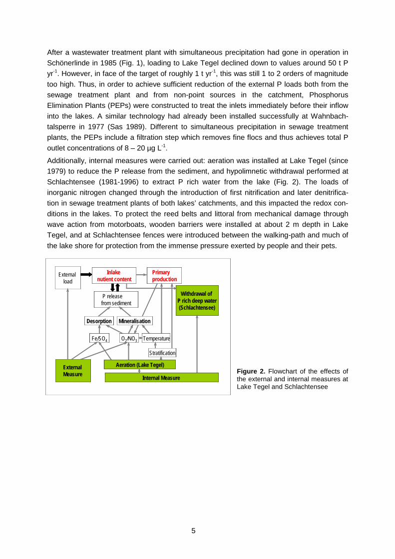
Additionally, internal measures were carried out: aeration was installed at Lake Tegel (since 1979) to reduce the P release from the sediment, and hypolimnetic withdrawal performed at Schlachtensee (1981-1996) to extract P rich water from the lake (Fig. 2). The loads of inorganic nitrogen changed through the introduction of first nitrification and later denitrifica-tion in sewage treatment plants of both lakes’ catchments, and this impacted the redox con-ditions in the lakes. To protect the reed belts and littoral from mechanical damage through wave action from motorboats, wooden barriers were installed at about 2 m depth in Lake Tegel, and at Schlachtensee fences were introduced between the walking-path and much of the lake shore for protection from the immense pressure exerted by people and their pets.

Figure 2. Flowchart of the effects of the external and internal measures at Lake Tegel and Schlachtensee

Ableitung von

(Schlachtensee)

produktionim See

dem Sediment

Desorption Mineralisation

Temperatur

Schichtung

Fe/SO4 O2/NO3

Belüftung (Tegeler See)Sanierung

Restaurierung

Withdrawal of P rich deep water(Schlachtensee)

External load

Primary production

Inlake nutient content

P release from sediment


Temperature

Stratification

Fe/SO4 O2/NO3

Aeration (Lake Tegel)External Measure Internal Measure

Ableitung von

(Schlachtensee)

produktionim See

dem Sediment


Temperatur

Schichtung

Fe/SO4 O2/NO3

Belüftung (Tegeler See)Sanierung

Restaurierung

Withdrawal of P rich deep water(Schlachtensee)

External load

Primary production

Inlake nutient content

P release from sediment


Temperature

Stratification

Fe/SO4 O2/NO3

Aeration (Lake Tegel)External Measure Internal Measure

6

3. Data compilation Inke Schauser and Ingrid Chorus

In addition to the data of the Umweltbundesamt, available for Schlachtensee since 1980 and for Lake Tegel since 1984, sampling was conducted as part of the OLIGO project from 2003-2006 at least at monthly intervals at both lakes for data on Secchi depth, vertical profiles of temperature, pH-, redox conditions, the concentrations of oxygen, total and soluble reactive phosphorus, nitrate, ammonia, chlorophyll-a, as well as an integrated epilimnetic sample for determining phytoplankton species composition and their biomass. At Schlachtensee, during some years this was intensified during summer stratification to obtain vertical profiles of temperature and oxygen concentrations at fortnightly intervals.

All data were made readily accessible for evaluation in a data base. Towards the end of OLIGO other projects such as Aquashift (funded by DFG) and CLIME (funded by EU) indicated the value of continuing this meanwhile long-term data set, so that this data base is likely to be valuable for future work. For Lake Tegel, the collaboration in OLIGO with the routine sampling program conducted by the Berliner Senatsverwaltung resulted in a decision to include vertical profiles with a similar resolution as in OLIGO in order to continue the data base after the end of OLIGO.

Methods for physico-chemical analyses are described in in Chorus and Schlag (1993) and in Lindenschmidt and Chorus (1998); for phytoplankton analyis see chapter 4.2.2.

Figure 3. Restoration history (curriculum vitae) for the different measures at Lake Tegel (1984-2006) and Schlachtensee (1980-2006) compared to the total phosphorus (TP) content in the upper and lower volume of the lakes.

1980 1982 1984 1986 1988 1990 1992 1994 1996 1998 2000 2002 2004 20060,0

0,2

0,4

0,6

0,8

1,01984 1986 1988 1990 1992 1994 1996 1998 2000 2002 2004 2006

Upper volume0-8 m Lake Tegel0-5 m Schlachtensee

0

4

8

12

16

20

Lower volume8-16 m Lake Tegel5-9 m Schlachtensee

Lake Tegel

Schlachtensee

TP in 1000 kg

PEP start

PEP startReduced PEP discharge

Temporal hypolimnion aerationPermanent aeration Temporal aeration

WTP without N treatment WTP denitrificationWTP nitrification

Storm water diversion

Makrophyte and reed planting

Fish kill Fish exstraction

Hypolimnetic withdrawal (HWD) HWD

WTP = Waste watertreatment plant

Slight reed increase

1980 1982 1984 1986 1988 1990 1992 1994 1996 1998 2000 2002 2004 20060,0

0,2

0,4

0,6

0,8

1,0

0,0

0,2

0,4

0,6

0,8

1,01984 1986 1988 1990 1992 1994 1996 1998 2000 2002 2004 2006

Upper volume0-8 m Lake Tegel0-5 m Schlachtensee

0

4

8

12

16

20

0

4

8

12

16

20

Lower volume8-16 m Lake Tegel5-9 m Schlachtensee

Lake Tegel

Schlachtensee

TP in 1000 kg

PEP start

PEP startReduced PEP dischargeReduced PEP discharge

Temporal hypolimnion aerationPermanent aeration Temporal aeration Temporal hypolimnion aerationPermanent aeration Temporal aeration

WTP without N treatment WTP denitrificationWTP nitrificationWTP without N treatment WTP denitrificationWTP nitrification

Storm water diversionStorm water diversion

Makrophyte and reed plantingMakrophyte and reed planting

Fish kill Fish exstractionFish kill Fish exstraction

Hypolimnetic withdrawal (HWD) HWD Hypolimnetic withdrawal (HWD) HWD

WTP = Waste watertreatment plant

Slight reed increaseSlight reed increase

7

Additionally, data were obtained from the Berliner Senatsverwaltung, Berliner Wasserbetriebe (PEP Tegel, PEP Beelitzhof, Wasserwerk Tegel), the Meteorological Institute of the Free University of Berlin, and extracted from literature. External data were particularly important for tributary flows, water extraction and for ions to use as markers to model the water budget. Meteorological data were obtained to model the hydrophysics and to test a current model predicting the phytoplankton development of the lakes. All available pertinent data were collated in a data base for further evaluation. Since the data were in different temporal and spatial scales, including data gaps, much work was invested to harmonise their format into monthly mean values for the total, the upper and lower volume of the lakes. Furthermore, for each lake, a curriculum vitae was established to compile the information on all of the management measures undertaken (Fig. 3).

8

4. Long term time series analysis

4.1 Restoration responses of the phosphorus budgets

4.1.1 Magnitude of external load reduction and assessment of inlake P response Inke Schauser and Bernd Heinzmann

The Phosphorus Elimination Plant (PEP) Beelitzhof was designed to treat the entire volume of water (up to 0.35 m3 s-1) pumped from the River Havel into lake Schlachtensee (Heinzmann and Sarfert 1990). This PEP began operation in autumn 1981, and in principle it works the same way as the PEP at Lake Tegel.

The PEP for Lake Tegel was built 1985 at the confluence of the 2 inflows, Nordgraben and Tegeler Fließ, shortly upstream of Lake Tegel. The PEP has the capacity to treat the complete volume (up to 6 m³ s-1) of this inflow under normal-to-moderate conditions, while storm water flows (up to 2.4 m³ s-1) that exceed this capacity can be bypassed through a pipe directly to the River Havel to avoid untreated water entering the lake (Heinzmann et al. 1991). The PEPs apply a four step process: precipitation/coagulation/flocculation sedi-mentation post precipitation filtration. The PEPs reduce the total P concentration at the lakes’ inlets by 1-2 orders of magnitude from up to 5 mg L-1 down to 8 - 20 µg P L-1.

1 course screen 7 backwash water tank 11 dissolution- and dosing equipment 2 fine screen 8 outflow for liquid coagulants 3 distribution tower 9 dissolution- and dosing 12 inlet basin 4 sedimentation tank equipment for coagulation 13 sand traps 5 filter 10 dissolution- and dosing 14 weir 6 filtrate- and flushing equipment for granulated water tank coagulants

Figure 4. PEP Tegel (Berlin): Scheme of the surface water treatment process (Heinzmann et al. 1991)

The scheme of the surface water treatment process is shown in Figure 4 for the PEP at Lake Tegel. The mechanical pre-purification comprises coarse screening (25 mm mesh size) and sedimentation of sand and larger particles in the inlet basin. Further, the water flows through

9

a fine screen (8 mm mesh size) to the raw water pumps. From here it is pumped to the distribution tower. The coagulants are directly dosed into the two pipes (pipe flocculation). To support rapid and complete mixing, the coagulants are dosed through nozzles at 4 points at which the two pipes are narrowed from 1 m to 0.7 m and then again extended to 1 m. On the way to the distribution tower micro flocks build up. After the distribution of the water to 6 pipes (diameter 1.2 m) a coagulant aid is added to support the macro flocculation process. Two pipes lead to each of the three sedimentation tanks in which the macro flocks settle. The sludge is removed into sludge traps by scrapers. The treated water flows down to 6 filters, which are situated under the sedimentation tanks. Additionally, there is the possibility for a second dosage step (post precipitation) in the clear water outflow tank before the filters. In the filters, the particles and flocks are removed in a double layer system with a filtration velocity of approximately 6 m h-1. The upper layer consists of 600 mm pumice gravel with a diameter of 2.5 - 3.1 mm. Under this layer a 1300 mm sand layer (diameter 0.71 -1.25 mm) is arranged. Approximately every 24 hours the filters have to be backwashed. The treatment costs including capital cost at both PEPs are approximately 0.09 – 0.18 € per m3 treated surface water (Heinzmann et al. 1991, Heinzmann & Sarfert 1990).

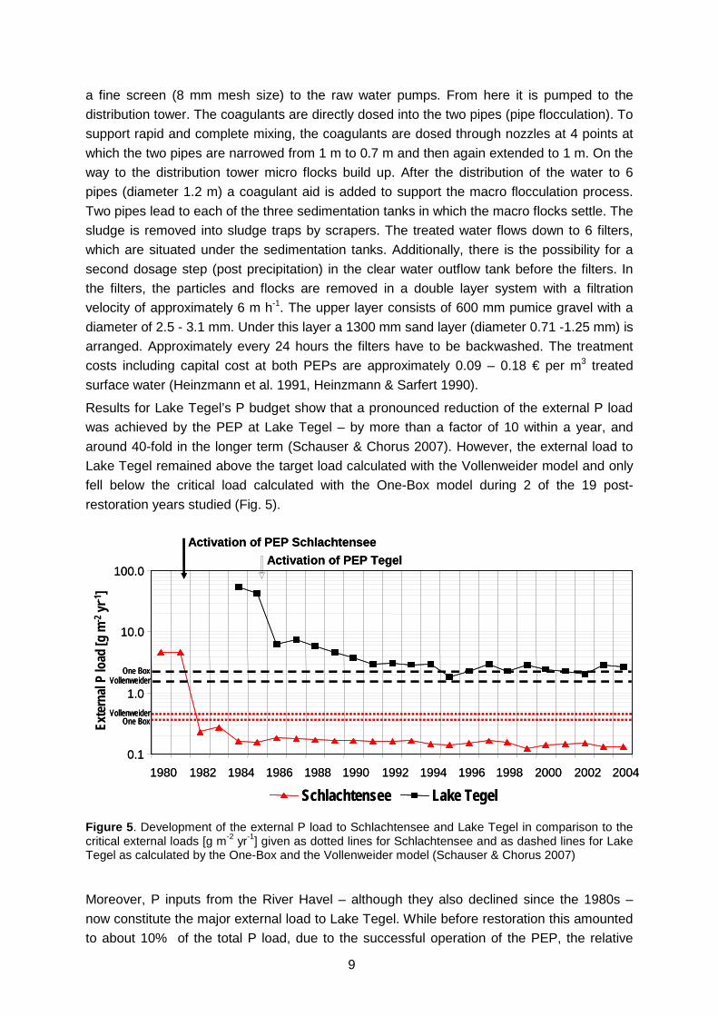
Results for Lake Tegel’s P budget show that a pronounced reduction of the external P load was achieved by the PEP at Lake Tegel – by more than a factor of 10 within a year, and around 40-fold in the longer term (Schauser & Chorus 2007). However, the external load to Lake Tegel remained above the target load calculated with the Vollenweider model and only fell below the critical load calculated with the One-Box model during 2 of the 19 post-restoration years studied (Fig. 5).

Figure 5. Development of the external P load to Schlachtensee and Lake Tegel in comparison to the critical external loads [g m-2 yr-1] given as dotted lines for Schlachtensee and as dashed lines for Lake Tegel as calculated by the One-Box and the Vollenweider model (Schauser & Chorus 2007)

Moreover, P inputs from the River Havel – although they also declined since the 1980s – now constitute the major external load to Lake Tegel. While before restoration this amounted to about 10% of the total P load, due to the successful operation of the PEP, the relative

0.1

1.0

10.0

100.0

1980 1982 1984 1986 1988 1990 1992 1994 1996 1998 2000 2002 2004

Schlachtensee Lake Tegel

Exte

rnal

P lo

ad[g

m-2

yr-1

]

Activation of PEP TegelActivation of PEP Schlachtensee

Vollenweider

VollenweiderOne Box

One Box

0.1

1.0

10.0

100.0

1980 1982 1984 1986 1988 1990 1992 1994 1996 1998 2000 2002 2004

Schlachtensee Lake Tegel

Exte

rnal

P lo

ad[g

m-2

yr-1

]

Activation of PEP TegelActivation of PEP Schlachtensee

Vollenweider

VollenweiderOne Box

One BoxVollenweider

VollenweiderOne Box

One Box

10

share of the external load originating from P transported into the lake by the River Havel has shifted to currently around 80% (2000–2004; Fig. 6).

Figure 6. External P load to Lake Tegel from Nordgraben/Tegeler Fließ and River Havel [t yr-1]

As described in Schauser et al. (2006a), Lake Tegel responded to the pronounced reduction in external P loading with an immediate and nearly exponential decline in total P concentrations in the water column during the first years (Fig. 7, upper panel). This recovery started to level out at P concentrations around 100 µg L-1, i.e. at a level just low enough to slightly reduce the biomass of algae and cyanobacteria (quantified in terms of Chl-a concentration). Only in 1993, 8 years after the reduction measures started, did total P concentrations decline further, along with a pronounced decline in Chl-a concentrations (Fig. 7, lower panel). Since then, P concentrations in the lake have ranged between 23 and 224 µg L–1 and concentrations of chlorophyll-a were well below 20 µg L-1 for most of the year, with spring or summer maxima sometimes approaching 50 µg L-1 as compared to 100-200 µg L-1 in earlier years. In consequence, transparency increased strongly, Secchi disc readings of less than 1 m are no longer recorded, and usually they are well above 2 m.

Figure 7. Total phosphorus concentrations and biomass of phytoplankton (algae + cyanobacteria, quantified in terms of chlorophyll-a concentrations) in Lake Tegel in µg L-1 in 1 m depth, monthly means (modified from Schauser et al. 2006a)

0

40

80

120

160

1984 1986 1988 1990 1992 1994 1996 1998 2000 2002 2004

0

40

80

120

160

1984 1986 1988 1990 1992 1994 1996 1998 2000 2002 2004

Nordgraben/Tegeler Fließ River HavelNordgraben/Tegeler Fließ River Havel

Exter

nalP

load

[t yr

-1]

Activation of PEP TegelActivation of PEP Tegel

0

200

400

600

800

1000

1984 1986 1988 1990 1992 1994 1996 1998 2000 2002 2004 20060

50

100

150

200

250

TP [µ

g L-1

]

Chl

-a[µ

g L-1

]

Activation of PEP Tegel Lake Tegel, 1 m

0

200

400

600

800

1000

1984 1986 1988 1990 1992 1994 1996 1998 2000 2002 2004 20060

50

100

150

200

250

0

200

400

600

800

1000

1984 1986 1988 1990 1992 1994 1996 1998 2000 2002 2004 20060

50

100

150

200

250

TP [µ

g L-1

]

Chl

-a[µ

g L-1

]


TP [µ

g L-1

]

Chl

-a[µ

g L-1

]


11

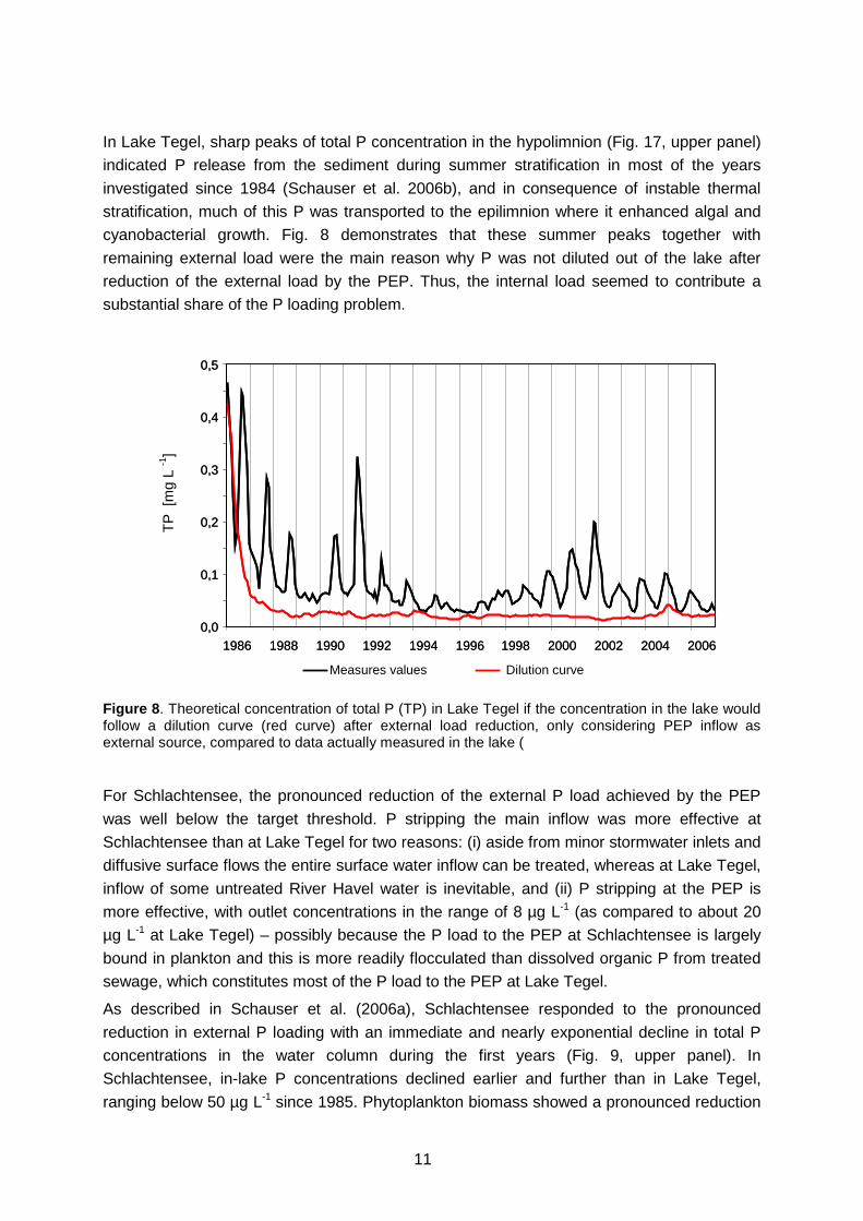
In Lake Tegel, sharp peaks of total P concentration in the hypolimnion (Fig. 17, upper panel) indicated P release from the sediment during summer stratification in most of the years investigated since 1984 (Schauser et al. 2006b), and in consequence of instable thermal stratification, much of this P was transported to the epilimnion where it enhanced algal and cyanobacterial growth. Fig. 8 demonstrates that these summer peaks together with remaining external load were the main reason why P was not diluted out of the lake after reduction of the external load by the PEP. Thus, the internal load seemed to contribute a substantial share of the P loading problem.

Figure 8. Theoretical concentration of total P (TP) in Lake Tegel if the concentration in the lake would follow a dilution curve (red curve) after external load reduction, only considering PEP inflow as external source, compared to data actually measured in the lake (

For Schlachtensee, the pronounced reduction of the external P load achieved by the PEP was well below the target threshold. P stripping the main inflow was more effective at Schlachtensee than at Lake Tegel for two reasons: (i) aside from minor stormwater inlets and diffusive surface flows the entire surface water inflow can be treated, whereas at Lake Tegel, inflow of some untreated River Havel water is inevitable, and (ii) P stripping at the PEP is more effective, with outlet concentrations in the range of 8 µg L-1 (as compared to about 20 µg L-1 at Lake Tegel) – possibly because the P load to the PEP at Schlachtensee is largely bound in plankton and this is more readily flocculated than dissolved organic P from treated sewage, which constitutes most of the P load to the PEP at Lake Tegel.

As described in Schauser et al. (2006a), Schlachtensee responded to the pronounced reduction in external P loading with an immediate and nearly exponential decline in total P concentrations in the water column during the first years (Fig. 9, upper panel). In Schlachtensee, in-lake P concentrations declined earlier and further than in Lake Tegel, ranging below 50 µg L-1 since 1985. Phytoplankton biomass showed a pronounced reduction

0,0

0,1

0,2

0,3

0,4

0,5

1986 1988 1990 1992 1994 1996 1998 2000 2002 2004 2006

Measures values Dilution curve

In-la

keP

[mg/

L]

0,0

0,1

0,2

0,3

0,4

0,5

1986 1988 1990 1992 1994 1996 1998 2000 2002 2004 2006

Measures values Dilution curve

In-la

keP

[mg/

L]

TP [

mg

L -1

]

12

for the first time in 1985, just 4 years after restoration started (Fig. 9, lower panel) and since 1993, no Chl-a maxima >20 µg L-1 were observed in the lake’s epilimnion.

Figure 9. Total phosphorus concentrations and biomass of phytoplankton (algae + cyanobacteria, quantified in terms of chlorophyll-a concentrations) in Schlachtensee in µg L-1 in 1 m depth, monthly means; shaded bar indicates data gap for the first half of 2003 (modified from Schauser et al. 2006a)

As in Lake Tegel, in Schlachtensee the patterns of P concentration in the hypolimnion indicated both accumulation of total P from sinking plankton organisms and detritus, as well as P release from the sediment at the end of the summer stratification (Schauser et al. 2006b); thus, the internal load seemed to be part of the P loading problem. However, total P concentrations in the lake developed much closer to the theoretical dilution curve (Fig. 10) than in Lake Tegel, indicating internal loading to be less of a problem.

Figure 10. Theoretical concentration of total P (TP) in Schlachtensee if the concentration in the lake would follow a dilution curve (red curve) after external load reduction compared to data actually measured in the lake; the shaded bar indicates data gap for the first half of 2003

0

200

400

600

800

1000

1980 1982 1984 1986 1988 1990 1992 1994 1996 1998 2000 2002 2004 20060

50

100

150

200

250Schlachtensee, 1 mActivation of PEP Beelitzhof

TP [µ

g L-1

]

Chl

-a[µ

g L-1

]

0

200

400

600

800

1000

1980 1982 1984 1986 1988 1990 1992 1994 1996 1998 2000 2002 2004 20060

50

100

150

200

250

0

200

400

600

800

1000

1980 1982 1984 1986 1988 1990 1992 1994 1996 1998 2000 2002 2004 20060

50

100

150

200

250Schlachtensee, 1 mActivation of PEP Beelitzhof

TP [µ

g L-1

]

Chl

-a[µ

g L-1

]

Schlachtensee, 1 mActivation of PEP Beelitzhof

TP [µ

g L-1

]

Chl

-a[µ

g L-1

]

0

0,1

0,2

0,3

0,4

1982 1984 1986 1988 1990 1992 1994 1996 1998 2000 2002 2004

Measured values Dilution curve

In-la

keP

[mg/

L]

0

0,1

0,2

0,3

0,4

1982 1984 1986 1988 1990 1992 1994 1996 1998 2000 2002 2004

Measured values Dilution curve

In-la

keP

[mg/

L]

TP [

mg

L -1

]

13

PEP Tegel

4.1.2 Assessment of internal measures Inke Schauser

Aeration at Lake Tegel As internal measure, 15 aerators were installed throughout the main basin in 1979 in Lake Tegel (Fig. 11), originally to counteract dramatic oxygen depleation which climbed up to 4 m depth during summer. Later they continued to be used as internal measure to support trophic recovery, with the aim to oxygenate the hypolimnion and the sediment surface in order to keep phosphorus (P) locked in the sediment and thus to reduce internal loading. This measure was based on the assumption that anoxic desorption of P is a potentially relevant source of internal P loading.

Figure 11. Map of Lake Tegel with locations of the Phosphorus Elimination Plant (PEP) and of the aerators (shaded areas: islands)

The periods and intensity of aeration were different over the years. Until 1989, it is not known how many aerators were in use at which point in time or whether the large, the small, or both compressors were in operation, although in principle, aeration was intended to be continuous. Because the aerators strongly affected the stability of the lake’s thermal stratification (Lindenschmidt & Chorus 1997), their operation in subsequent years was restricted to periods when oxygen depletion in the hypolimnion emerged. In 1991, very unusual weather conditions prevented stratification of the lake. From 1992 to 1998, aeration was almost completely avoided. Furthermore, beginning in 1996 the aerators were modified to oxidise only the hypolimnion without disturbing stratification. On this basis, their operation was increased again starting 1999.

Comparing the development of hypolimnetic P concentration with periods of aeration operation does not indicate a relationship (Fig. 12). Here, only the years since 1989 are shown because before that year, the aerators were in operation throughout the stagnation period. In most years the P concentration in the hypolimnion also increased during aeration. Results of sediment analysis show a ratio of iron to phosphorus of around 1 to 5 (Schauser et al. 2006b), whereas since the work of Jensen et al. (1992) it is clear that effective aerobic adsorption of P to iron requires a ratio above the range of 15. Thus, sediments in Lake Tegel

14

appear to have only a weak potential for adsorptive binding of iron. Rather, aerobic mineralisation of organic material (enhanced by elevated temperatures) is probably the main source for P release from the sediments (see Chapter 4.1.3).

Figure 12. Mean total P concentration in the upper (0-8 m lake depth) and lower (8–15 m lake depth) compartment of Lake Tegel, compared with the times and intensities of aeration (1989–2004) (Schauser & Chorus 2007)

An indicator of whether sediments act as source or sink of P is the annual net sedimentation factor (Fig. 13). A positive value indicates that the sediment is acting as a P sink, a negative value indicates that on an annual basis the sediment is a P source. For Lake Tegel, the net sedimentation factor changed considerably after 1984 from above 5 (1984 and 1985, but also in 1989 and 1996) to less than -1 (1986, 1987, 1990) or even below -4 (1991). The development of the net sedimentation factor and the length of the annual aeration periods do not show a strong relationship, although data for the years after 1991 even suggest some inverse pattern, i.e. more P release with more days of aeration.

To test whether stratification stability impacts on P release from the sediments, we used the temperature difference between 1 and 14 m as an indicator for stratification stability and compared it to the net sedimentation factor (Fig. 13). The annual mean temperature difference between the surface and bottom waters proved to be closely related to the aeration activity, in Lake Tegel, and after 1992, it was always greater than 3 °C. However, it showed little relationship to the net sedimentation factor, which was apparently largely controlled by other factors.

15

Activation of PEP Tegel

-6

-4

-2

0

2

4

6

1984 1986 1988 1990 1992 1994 1996 1998 2000 2002 20040

50

100

150

200

250

300

350

400Ne

t sed

imen

tatio

n fa

ctor

[yr-1

]Te

mpe

ratu

re d

iffer

ence

1-14

m [°

C]

Days of aeration[d yr -1]

Temperature differenceNet sedimentation coefficent Days of aeration

Activation of PEP TegelActivation of PEP Tegel

-6

-4

-2

0

2

4

6

1984 1986 1988 1990 1992 1994 1996 1998 2000 2002 20040

50

100

150

200

250

300

350

400Ne

t sed

imen

tatio

n fa

ctor

[yr-1

]Te

mpe

ratu

re d

iffer

ence

1-14

m [°

C]

Days of aeration[d yr -1]

Temperature differenceNet sedimentation coefficent Days of aerationNet sedimentation factor

Figure 13. Net sedimentation factor [yr-1], annual mean temperature difference between 1m and 14 m lake depth [°C] and days of aeration per year [d yr-1] in Lake Tegel. Negative values for the net sedimentation factor indicate sediments to be a source for P, positive values indicate them to be a sink for P

As hypolimnetic aeration did not show any positive impact on the P budget, aerator operation now chiefly targets maintaining oxygen at levels which are sufficient for fish fry and benthic organisms in sediment-near water-layers. Also, this measure enhances biodegradation of sedimented organic material.

Hypolimnetic Withdrawal at Schlachtensee To accelerate Schlachtensee’s response to external load reduction, from 1981 to 1996 hypolimnetic water was pumped out of the deepest basin of the lake near its deepest point for a period of several weeks toward the end of summer stratification (Fig. 14). This measure was easily implemented, using the pipe already installed from the PEP to the lake and merely running it in reverse direction for a few weeks. The water was pumped into Wannsee, which is part of the River Havel System. There it caused no impact because of its comparatively small volume.

However, the hypolimnion of Schlachtensee is rather small, amounting to only around 20% of the volume of the whole lake and 10% of the annual water outflow. While the depth of the withdrawal pipe was not precisely defined, we assume that withdrawal took place in the hypolimnion below a depth of 6 m. Estimates of the amount of P withdrawn are hampered by the steep P concentration gradient at the mouth of the pipe and a poor understanding of the precise water-layer extracted. Nonetheless, even if we assume an error of 100% caused by this uncertainty, results are clear: Especially in the first 2-3 years of restoration, the hypolimnetic withdrawal increased the P outflow factor considerably, although due to the small volume of the hypolimnion, the withdrawal pipe could be operated only a few weeks a year. In 1981, the withdrawal exported around 200 kg P of the lake’s ~1300 kg P content. However, the comparison between the P content in the lake, the external P load, and the P withdrawn from the hypolimnion (Fig. 15) shows in later years that the hypolimnetic

16

withdrawal had only a minor effect on the total P budget of the lake. Both the absolute amounts of P exported and their relative share of the P content rapidly decreased to 78 kg P in 1982, 18 kg P in 1983, and 10 kg P in 1984, and in 1996 only 2 kg of the lake’s ~40 kg total P content. This amounted to little more than 3% of the lake’s P content, and in comparison, the annual external load reduction after 1981 was around 1900 kg.

Figure 14. Map of Schlachtensee with bathy-metric lines, the position of PEP and that of hypo-limnetic withdrawal (Schauser & Chorus 2007)

Figure 15. P content [kg], external P load [kg yr-1] and P withdrawn from the hypolimnion, [kg yr-1] of Schlachtensee (error bars indication withdrawal in either 6 or 7.5 m depth; Note the logarithmic scale) (Schauser & Chorus 2007)

0

1

10

100

1000

10000

1980 1982 1984 1986 1988 1990 1992 1994 1996 1998 2000 2002 2004

P in the lake [kg] external P load [kg a-1] P withdrawn [kg a-1]

0

1

10

100

1000

10000

1980 1982 1984 1986 1988 1990 1992 1994 1996 1998 2000 2002 2004

P in the lake [kg] external P load [kg a-1] P withdrawn [kg a-1]

17

4.1.3 Causes and thresholds for P release from the sediment Inke Schauser

The most important phosphorus (P) mobilization processes in sediments are mineralization of organically bound P and desorption/dissolution of redox-sensitively bound P (Fig. 16). Mobilization is followed by diffusive or advective transport of the dissolved P out of the sediment. While mineralization is a temperature-controlled process, desorption/dissolution of redox-sensitively bound P is mainly redox-controlled. Mineralization is accompanied by reduction of – in this sequence – oxygen, nitrate, manganese oxide, iron(III), sulphate, and lastly a production of methane. As phosphate is adsorbed to iron(III), its reduction to iron(II) leads to desorption. Sulphate affects desorption because it gets reduced to sulphide which bounds iron under anaerobic conditions permanently as iron-sulphide. Therefore, the use of sulphate salts to precipitate phosphate in the PEP can enhance P desorption from the sediment. Thus, mineralization results both in direct P mobilization, and further in an indirect mobilization in consequence of increased desorption due to the decreased redox potential.

Figure 16. Effect of temperature and oxygen on the P release from sedi-ments (+ indicates increasing influence, - indicates decreasing influence)

To improve the understanding of the sediment processes, in summer 2004 in situ porewater investigations and sediment core analyses of both lakes were performed by Leibniz-Institut of Freshwater Ecology and Inland Fisheries (IGB) in the context of a subcontract. In late summer of 2006, additional sediment columns were taken from Lake Tegel and were investigated experimentally in the laboratory by IGB (subcontract to Dr. Hupfer) for P release under the influence of artificial aeration.

Both lakes reacted differently to the external load reduction (Schauser et al. 2006b). In Schlachtensee the presence of nitrate above the sediment suppressed P release quite regularly. This is in line with the chemical composition of the sediment, since the Fe/P ratio is sufficiently high to provide enough aerobic sorption capacity in Schlachtensee. Here, sediment P release is dominated by desorption due to FeS precipitation (Fig. 17, upper panel). Furthermore, the observations at Schlachtensee confirm a threshold for nitrate-N suppressing P release to be in the range of 0.5 mg/L.

Organically bound P P sorbed at Fe

P-Release

Mineralisation Desorption

+

Temperature

+ ++

Temperature

++

Oxygen

+ -

Oxygen

++ --

---

18

Schlachtensee

Lake Tegel

Figure 17. Temperature, nitrate and phosphorus in 7.5 m depth in Lake Schlachtensee (upper panels) and in 15 m depth in Lake Tegel (lower panels). Periods of maximum P concentrations are marked red. Dotted horizontal lines mark nitrate-N threshold values for P release, and gray shading for Schlachtensee marks a 6-month data gap (Schauser et al 2006b, modified). Note the differences between both lakes in scales of the axes for nitrate and TP

00.5

11.5

22.5

3

1990 1991 1992 1993 1994 1995 1996 1997 1998 1999 2000 2001 2002 2003 2004

mg

P L-1

TP3.5

0

2

4

6

8

10

NO3-N

mg

L-1N

0

5

10

15

20

25

Temperatur

°C

00.5

11.5

22.5

3

1990 1991 1992 1993 1994 1995 1996 1997 1998 1999 2000 2001 2002 2003 2004

mg

P L-1

TP3.5

00.5

11.5

22.5

3

1990 1991 1992 1993 1994 1995 1996 1997 1998 1999 2000 2001 2002 2003 20041990 1991 1992 1993 1994 1995 1996 1997 1998 1999 2000 2001 2002 2003 2004

mg

P L-1

TP3.5

0

2

4

6

8

10

NO3-N

mg

L-1N

0

2

4

6

8

10

0

2

4

6

8

10

NO3-N

mg

L-1N

0

5

10

15

20

25

Temperatur

°C

0

5

10

15

20

25

Temperatur

°C

T

P

Tem

pera

ture

NO

3–N

[m

g L-1

]

[°C

]

[m

g L-1

]

m

g P

L-1

TP

mg

L-1N

0

0.5

1

1.5

2

2.5

NO3-N

0

0.05

0.1

0.15

0.2

0.25

1990 1991 1992 1993 1994 1995 1996 1997 1998 1999 2000 2001 2002 2003 2004

0

5

10

15

20

Temperatur

°Cm

g P

L-1

TP

mg

L-1N

0

0.5

1

1.5

2

2.5

NO3-N

0

0.05

0.1

0.15

0.2

0.25

1990 1991 1992 1993 1994 1995 1996 1997 1998 1999 2000 2001 2002 2003 2004

0

5

10

15

20

Temperatur

°Cm

g P

L-1

TP

mg

L-1N

0

0.5

1

1.5

2

2.5

NO3-N

mg

L-1N

0

0.5

1

1.5

2

2.5

NO3-N

0

0.05

0.1

0.15

0.2

0.25

1990 1991 1992 1993 1994 1995 1996 1997 1998 1999 2000 2001 2002 2003 20040

0.05

0.1

0.15

0.2

0.25

1990 1991 1992 1993 1994 1995 1996 1997 1998 1999 2000 2001 2002 2003 20041990 1991 1992 1993 1994 1995 1996 1997 1998 1999 2000 2001 2002 2003 2004

0

5

10

15

20

Temperatur

°C

0

5

10

15

20

0

5

10

15

20

Temperatur

°C

Temperatur

°C

Temperatur

°C

T

P

Tem

pera

ture

NO

3–N

[m

g L-1

]

[°C

]

[mg

L-1]

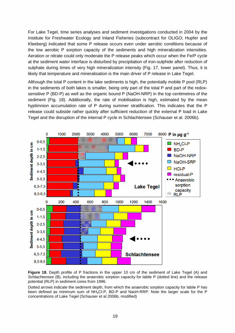
19

For Lake Tegel, time series analyses and sediment investigations conducted in 2004 by the Institute for Freshwater Ecology and Inland Fisheries (subcontract for OLIGO; Hupfer and Kleeberg) indicated that some P release occurs even under aerobic conditions because of the low aerobic P sorption capacity of the sediments and high mineralization intensities. Aeration or nitrate could only moderate the P release peaks which occur when the Fe/P cycle at the sediment water interface is disturbed by precipitation of iron-sulphide after reduction of sulphate during times of very high mineralization intensity (Fig. 17, lower panel). Thus, it is likely that temperature and mineralisation is the main driver of P release in Lake Tegel.

Although the total P content in the lake sediments is high, the potentially mobile P pool (RLP) in the sediments of both lakes is smaller, being only part of the total P and part of the redox-sensitive P (BD-P) as well as the organic bound P (NaOH-NRP) in the top centimetres of the sediment (Fig. 18). Additionally, the rate of mobilisation is high, estimated by the mean hyplimnion accumulation rate of P during summer stratification. This indicates that the P release could subside rather quickly after sufficient reduction of the external P load in Lake Tegel and the disruption of the internal P cycle in Schlachtensee (Schauser et al. 2006b).

Figure 18. Depth profile of P fractions in the upper 10 cm of the sediment of Lake Tegel (A) and Schlachtensee (B), including the anaerobic sorption capacity for labile P (dotted line) and the release potential (RLP) in sediment cores from 1996. Dotted arrows indicate the sediment depth, from which the anaerobic sorption capacity for labile P has been defined as minimum sum of NH4Cl-P, BD-P and NaoH-RRP. Note the larger scale for the P concentrations of Lake Tegel (Schauser et al 2006b, modified)

20

For Lake Tegel the results gleaned from the analysis of the field data time series and P binding forms were supplemented with laboratory experiments conducted with sediment columns by the Institute for Freshwater Ecology and Inland Fisheries (subcontract for OLIGO; Hupfer and Kleeberg) in 2006. These addressed the effects of oxygen and sulphate availability on the P release. While taking sediment cores into the laboratory changes some conditions (such as pressure and sediment-water interaction) such experiments allow more detailed insights into mechanisms influencing P-binding and –release. The results show:

1. Temperature controls the mineralisation intensity of organic material.

Although the overall oxygen consumption is independent of temperature, thus only controlled by oxygen supply, the depth of oxygen penetration depends on temperature. No conclusion can be drawn in which way oxygen availability influences the mineralisation intensity.

2. The sediment theoretically contains enough iron to prevent P release and support further uptake of P under aerobic conditions.

The total P sorption capacity of Lake Tegel sediment was determined to be high. However, this is only valid under laboratory conditions, i.e. where oxygen supply is sufficient to oxidise the top sediment layer and external P supply for the sediment is unlimited, with P concentrations in the water in the range of 2 mg L-1. Under in-situ conditions, P supply is limited by the P concentration of the lake water, varying between 30 and 700 µg L-1, and the oxygen supply is limited by the aerator capacities and transport processes in the water. These experiments did not show how much oxygen is needed to keep sediment aerobic. They cannot answer the question whether under anaerobic conditions the accumulated iron will be reduced and the P taken up will be released. Other experiments at lower P concentrations up to 500 µg L-1 in the water showed P release also under aerobic conditions.

3. Aeration is not likely to prevent P release, however it can reduce it.

In the laboratory, P release under anaerobic conditions was around 3 times higher than under aerobic conditions. Under aerobic conditions, some release occurs since the actual sorption capacity of the sediment is not high enough to prevent it: phosphorus and iron accumulate in the top layer as redox sensitive bound P and Fe, leaching out of the lower layers and moving upwards, whereas under anaerobic conditions iron precipitates in the lower layers as FeSx. Surprisingly, the iron mobility from deeper horizons towards the top layer was rather high in Lake Tegel sediments.

4. Higher sulphate concentrations increase sulphate reduction and P release rates.

The results of further experiments indicate that the sulphate penetration depth as well as the overall sulphate consumption depends on the sulphate supply. A higher sulphate reduction rate is coupled to an increase of Fe fixation and P mobility. In Lake Tegel sediments, sulphate reduction in lower sediment layers is not limited by availability of organic matter. In contrast, it is more likely that mineralisation is sulphate limited in deeper sediment layers. Aerobic conditions do not reduce the overall sulphate reduction rate, they only shift the sulphate reduction horizon into deeper layers, thus increasing the overall mineralisation rate. This has to be kept in mind, since the Phosphate Elimination Plant is discharging sulphate into Lake Tegel. Aeration will not be able to prevent increased sulphate reduction rates, since the organic material supply to Lake Tegel

21

sediments is too high. Aeration might still be able to counteract increased P release due to iron accumulation in the top sediment layer.

In conclusion for P-release from the sediment, for Schlachtensee the results confirm the assumed threshold of 0.5 mg/L NO3-N. For Lake Tegel the pool of redox-sensitive binding-partners for P – i.e. iron – and the amount of sulphate competing with P for Fe determine P release. In particular, they show that elevated temperatures may strongly enhance mineralisation, and mixing that increases hypolimnion temperatures is therefore best avoided (see also Chapter 6.1).

22

4.2 Restoration responses of the biota

4.2.1 Phytoplankton species response to oligotrophication Ingrid Chorus and Verena Niesel

The central target of the restoration of Schlachtensee and Lake Tegel was to reduce overall phytoplankton biomass, but in particular that of the most noxious taxa, the cyanobacteria. One aim of OLIGO was to analyse how phytoplankton responded to the pronounced decline of phosphorus concentrations, checking in particular which taxa followed non-linear and threshold patterns, as such information is of high relevance for planning restoration projects.

Methods Phytoplankton was sampled at the deepest site of each lake, both as grab sample for enumeration and with a plankton net of 10 µm mesh size. Grab samples either integrated the epilimnion (most cases) or were from 2 m depth to represent the epilimnion. These are pooled for the analysis shown in the following (as depth profiles of chlorophyll-a indicate that differences in vertical distribution within the epilimion were very pronounced in most situations; data not shown).

Species were identified with the help of the standard literature (chiefly Huber-Pestalozzi and Ettl) as well as in discussions with colleagues, particularly at IAP1

Enumeration was performed after sedimentation of 2–25 ml (depending on organism density) using an inverse microscope, usually at 400-fold magnification, counting at least 2 chamber bottom transects – and more if results between transects differed by >20% (Utermöhl 1958; Lawton et al. 1999). Enumeration attempted to achieve around 200 counts for each of the most frequent taxa or size categories, and categories with less than 20 counts were not included in the quantitative evaluation. For biovolume determination, in each sample 10-20 cells of each species were measured, until 2002 using an ocular micrometer and since then on the computer screen by mouse-clicking the image of a video camera. Prior to enumera-

meetings. Frequently species identification was uncertain, and we then quanitifed by genus (for some, differentiating by size categories to obtain more precise biovolume data). This was typically the case for Cryptophyta, of which many cells in a given sample can be identified, but the morphology of many others appears intermediate between two species. Likewise, some Microcystis colonies in a sample could be identified, but others remained unclear. Furthermore, for counting the cells colonies were disintegrated (see below) and thus cells could no longer be allocated to a species. For enumeration, we grouped all single-celled centric diatoms in 3 categories differentiated by size (diameters of > 15 µm, 8-15 µm and < 8 µm). Reynolds (1997) demonstrated that the surface/volume ratio and thus cell morphometry is a key determinant of nutrient uptake and light harvesting, and thus of growth rate. For an ecological assessment of the response of taxa of otherwise similar morphometry to changes in environmental conditions such as trophic state, turbidity or water-body mixing, size classes therefore are likely to provide an adequate differentiation.

1 IAP = International Association of Phytoplanktologists

23

tion, colonies of Microcystis and Anabaena were disintegrated by ultrasonication to enable counting of individual cells. For filamentous forms, rather than counting filaments we measured the full length of the fraction of each filament within the delineation of the transect.

Enumeration and biovolume determination were conducted in most, but not in all of the years sampled, in the context of a range of projects by different workers, with periodic comparison of counting results between workers. For 1984-1985 we include literature data by Ripl et al. (1990), and data for 1995/1996 are from Fastner (1999 and pers. com.).

For both lakes Katrina Laskus continuously evaluated plankton net samples until December 2003, starting in 1980 for Schlachtensee and in 1984 for Lake Tegel (with exception of a gap for Schlachtensee which was not sampled at all during the first half of 2002). These net samples integrated equal volumes of sample from each meter sampled (0 – 4 m for Schlach-tensee and 0 – 8 m for Lake Tegel), fixed with formaldehyde and sedimented in test tubes with a tapered end. Analysis for semi-quantitative comparison of occurrence differentiated between “single event” and 3 categories of relative frequency of observation, ranging from “occasional”, “frequent”, to “massive”.

While biovolume data are a more meaningful basis for assessing the restoration response of taxa, in the following we include the net plankton sample data particularly as indicator for the development of taxa in the years for which no biovolume data are available. For this purpose, we assigned an order of magnitude to each of the 3 frequency categories, using 0.01 (occasional) / 0.1 (frequent) and 1 (dominant) for most taxa; for large-celled (Ceratium; large centric diatoms; cyanobacteria) or bloom-forming taxa we assigned 0.1 / 1 / 10 to these relative frequencies.

For Schlachtensee, the figures in this chapter include all three categories, while for Lake Tegel we focused our analysis on the frequent and massive occurrences and used the net plankton data for occasional occurrence only to fill gaps where quantitative data are missing.

Conditions determining phytoplankton growth Fig. 19 gives an overview of the development of key conditions for phytoplankton growth in both lakes: the macronutrients nitrogen (as nitrate-N) and phosphorus (both as total and as soluble reactive P) as well as Secchi depths which indicate transparency and thus light availability. The bottom chart summarises growth conditions during summer: the darker the shading, the more of the resource is available, and the higher the stability of summer thermal stratification. Rather than reflecting calculated means over the summer period, these 4 categories of shading represent estimates gleaned from the curves over to roughly characterise the overall summer situation.

As proxy for stratification stability versus turbulence within the epilimnion, we used the tem-perature difference (Δ T) between the surface and a deeper layer (approximately the late summer metalimnion of each lake, i.e. 4 m for Schlachtensee and 8 m for Lake Tegel): large values for Δ T indicate pronounced thermal gradients within the epilimnion or even a shallow thermocline located above the mean thermocline depth for the respective lake – in both cases stable thermal stratification. Turbulence is relevant to phytoplankton in three ways: (i) It keeps species with high specific density – particularly diatoms – suspended, thus reducing their sedimentation loss rates. (ii) It entrains cells and colonies through light gradients, with

24

Figure 19. Hydrophysical and chemical growth conditions for phytoplankton

Years on X-axis indicate January 1st. Vertical hatched bars: data gaps. Panels give: Light availability as indicated by Secchi disk readings for tranparency Total and soluble reactive phosphorus (TP/SRP) as epilimnion means (Schlachtensee: 0-4 m: Lake Tegel: 0-8 m); concentrations >100 µg/L not shown. Total areas: TP, grey shading: SRP Nitrate-N as epilimnion means (Schlachtensee: 0-4 m: Lake Tegel: 0-8 m) Temperature gradients within the epilimnion (ΔT) as measure of stagnation versus turbulence Summary charts of growth conditions during summer: the darker the shading, the more of the resource is available, i.e. the higher the stability of summer thermal stratification

Lake Tegel

Schlachtensee

0

50

100

ΔT

0-8

m

NO

3-N

T

P/SR

P

Secc

hi[°

C]

[mg/

L]

[µ

g/L]

[m

]

0

4

8

-4048

12

84 85 86 87 88 89 90 91 92 93 94 95 96 97 98 99 00 01 02 03 04 05 06

0

2

4

84 85 86 87 88 89 90 91 92 93 94 95 96 97 98 99 00 01 02 03 04 05 06

NO3-N TPSRPSecchiΔT 0-8 m

0

50

100

0

1

2

ΔT

0-8

m

NO

3-N

T

P/SR

P

Secc

hi[°

C]

[mg/

L]

[µ

g/L]

[m

]0

2

4

80 81 82 83 84 85 86 87 88 89 90 91 92 93 94 95 96 97 98 99 00 01 02 03 04 05 06

NO3-NTPSRPSecchiΔT 0-4 m

-4048

80 81 82 83 84 85 86 87 88 89 90 91 92 93 94 95 96 97 98 99 00 01 02 03 04 05 06

Lake Tegel

Schlachtensee

0

50

100

ΔT

0-8

m

NO

3-N

T

P/SR

P

Secc

hi[°

C]

[mg/

L]

[µ

g/L]

[m

]

0

4

8

-4048

12

84 85 86 87 88 89 90 91 92 93 94 95 96 97 98 99 00 01 02 03 04 05 06

0

2

4

84 85 86 87 88 89 90 91 92 93 94 95 96 97 98 99 00 01 02 03 04 05 06


0

50

100

0

50

100

ΔT

0-8

m

NO

3-N

T

P/SR

P

Secc

hi[°

C]

[mg/

L]

[µ

g/L]

[m

]

0

4

8

0

4

8

-4048

12

84 85 86 87 88 89 90 91 92 93 94 95 96 97 98 99 00 01 02 03 04 05 06

0

2

4

84 85 86 87 88 89 90 91 92 93 94 95 96 97 98 99 00 01 02 03 04 05 06


0

50

100

0

50

100

0

1

2

0

1

2

ΔT

0-8

m

NO

3-N

T

P/SR

P

Secc

hi[°

C]

[mg/

L]

[µ

g/L]

[m

]0

2

4

80 81 82 83 84 85 86 87 88 89 90 91 92 93 94 95 96 97 98 99 00 01 02 03 04 05 060

2

4

80 81 82 83 84 85 86 87 88 89 90 91 92 93 94 95 96 97 98 99 00 01 02 03 04 05 06


-4048

80 81 82 83 84 85 86 87 88 89 90 91 92 93 94 95 96 97 98 99 00 01 02 03 04 05 06

25

deeper mixing implying more time spent in darker layers. (iii) Switches between phases of more turbulence and phases of quiescence may cause shifts in phytoplankton species dominance and biomass (Chorus and Schlag 1993).

Nitrogen: Lake Tegel receives nitrogen from sewage treatment in the catchment. Up to the autumn of 1985 this was largely from sewage irrigation fields, with some denitrification likely there and along the stream. Thus in Lake Tegel during summer epilimnion concentrations of nitrate-N dropped below 1 mg/L, as low as 0.08 mg /L in July of 1985 (Fig. 19). Nonetheless, concentrations of total inorganic N were never below 1 mg/L and usually above 2 mg/L (data not shown). After the sewage irrigation fields were replaced with a sewage treatment not yet including denitrification in late 1985, nitrate-N concentrations remained above 1 mg/L. Although denitrification was introduced in the late 1990’s, no potentially growth-limiting levels (below 0.15 mg/L) were observed since. Therefore, after 1985 we may consider nitrogen as irrelevant factor for phytoplankton growth limitation in Lake Tegel, as indicated by the black horizontal bar for nitrate in the summary chart (Fig. 19, bottom panel).

In Schlachtensee, up to 1983 summer concentrations of nitrate-N dropped to below the limit of detection (0.01 mg/L; Fig. 19). In 1984, they were below 0.15 mg/L only very briefly, and from 1985 to 1999, they always ranged well above 0.15 and usually above 0.4 mg/L. This increase reflects decreasing phytoplankton biomass, with more dissolved N being “left over” (indicated by black horizontal bars in the summary chart in Fig. 19). Since the end of the 1990s, nitrate concentrations decreased due to the introduction of sewage denitrification in the catchment, and potentially limiting concentrations below 0.15 mg/L occurred again, though only briefly and late in the growing season. Thus, the impact of N-limitation on seasonal succession of phytoplankton species in Schlachtensee was relevant largely before 1984.

Phosphorus: While the concentrations at which soluble reactive phosphorus (SRP) can limit P-uptake rates vary between species, generally concentrations above 10 µg/L are not likely to limit uptake rates. Thus, 5-10 µg/L have been used as threshold for P-limitation, however, with two caveats: one is the very rapid recycling of P already in the epilimnion: molecules liberated from degrading biomass are almost immediately taken up by phytoplankton cells. The other caveat is the capability of many phytoplankton species – particularly cyanobateria – to store phosphorus for up to 4 cell divisions. Thus, the most important information to be gleaned from the detection of SRP is that it is being “left over” by phytoplankton, this indicates P is not limiting. Prolonged phases of low SRP concentrations indicate that P may be limiting phytoplankton growth, but this remains uncertain. Therefore, total P (TP) is the relevant parameter for assessing how much biomass can be attained, and as discussed in chapter 8.3, both lakes show a threshold for TP-limitation of phytoplankton biomass below 50 µg/L TP.

In Lake Tegel, P concentrations first approached levels with some potential for impact on phytoplankton in 1989: SRP concentrations had already dropped below 10 µg/L briefly in 1986 -1988 (light-gray shading in Fig. 19), they were below 2 µg/L an extended summer phase in 1989, and TP briefly declined below 50 µg/L. Although concentrations increased again in winter, summer SRP has remained well below 2 µg/L for extended periods since 1988, sometimes interrupted by brief P pulses, and TP gradually declined to 25-30 µg/L in

26

1996. Exceptions are 1990 and 1991, when low stratification stability enhanced P-transport from the hypolimnion to the epilimnion, as well as some years during the phase of re-eutrophication when external P loads were higher, i.e. 1997 – 2001. During these periods, SRP was low (< 2 µg/L) only very briefly, and although summer TP remained below 30 µg/L, these phases became shorter from 1997 to 2001, until in 2002 the management regime was improved to reduce the external load again.

Thus, in Lake Tegel, some indication of P-limitation first became visible in 1988 (SRP-bars shaded grey in the summary chart for Lake Tegel in Fig. 19), and P was clearly limiting from 1993 to 1996. The set-back from 1997 to 2001 reduced phases with substantial P-limitation to short time spans in summer, while after 2002 these time spans increased again, with SRP < 2 µg/L at times possibly limiting uptake rates and TP < 30 µg/L clearly limiting carrying capacity for phytoplankton biomass.

In Schlachtensee, SRP first very briefly declined below 10 µg/L in 1982 and below 2 µg/L in 1983 and 1984. TP concentratios fell below 50 µg/L briefly in 1984. The decisive change occurred in 1985, with summer SRP below 4 µg/L and TP declining below 30 µg/L. Since 1988, summer SRP concentrations usually ranged from 1 to 2 µg/L and summer TP around 20 µg/L. Winter peaks declined substantially after 1997, and phases of summer TP in the range of 15 µg/L are becoming more prolonged since 2004. Thus, in Schlachtensee phos-phorus concentrations quite abruptly switched to substantial limitation in 1985 and have been very gradually decreasing further ever since, and the summary chart in Fig. 19 indicates pro-nounced P-limitation by the white horizontal bars for SRP since 1984 and for TP since 1986.

Light availability, i.e. water transparency (determined by Secchi disc readings) responded to decreased biomass in both lakes, more strongly in Schlachtensee than in Lake Tegel, reflecting the former’s more pronounced decline of phytoplankton biovolume. While Schlachtensee’s summer Secchi readings were ~ 0.5 m until 1985, they abruptly increased to > 1 m in 1985 and stayed > 2 m since 2000. This means that – assuming the euphotic depth to be 2.5 times the Secchi depth – that light penetrated down to the bottom of most of the water-body for most of the time (horizontal bars for “Secchi” in the summary charts in Fig. 19 accordingly switch from white – indicating little light availability for phytoplankton – before 1984 to black – indicating high light availability – after 1986).

In Lake Tegel, transparency was particularly low from 1984 to 1986 (before quantitative phytoplankton data are available; Fig. 19). During most of the lake’s hypertrophic phase, summer Secchi readings ranged from 0.5 to 1 m, with up to 2 m during the spring clearwater phase and sometimes in winter. Starting in 1994 with the decline of summer TP to ~ 30 µg/L, they were rarely less than 1 m, and readings of 2-4 m became characteristic for the clear-water phase as well as during winter. During the re-eutrophication phase (1997 – 2001), situations with less than 2 m Secchi-depth became more frequent again, and only by 2006 did summer Secchi depths remain above 2 m (with lower levels in spring).

Turbulence: For Schlachtensee, ΔT merely reflects differences in weather conditions between years, while in many years for Lake Tegel, it also reflects aerator operation (see Lindenschmidt and Chorus 1997); therefore years with more or less stability do not coincide for these two lakes.

27

Data for Schlachtensee show a phase with pronounced summer gradients from 1980-1987 and a phase of less stability from 1987-1995. After 1996, pronounced thermal gradients occur again in some years, but usually in spring rather than in summer. Lake Tegel’s ΔT pattern shows a more mixed epilimnion from 1984-1991, which up to 1990 is largely due to artificial destabilisation of thermal stratification through aeration (see Lindenschmidt and Chorus 1997 and for modelling results to differentiate between aeration and wind-driven mixing Lindenschmidt and Chorus 1998). 1991 had much stormy weather in spring, allowing less thermal stratification to develop in both lakes. Since 1992, aerator management in Lake Tegel minimised disruption of stratifycation, and indeed patterns for ΔT became more similar in both lakes. Years with less stable thermal gradients were 1999, 2001 and 2005. However, as Lake Tegel is much larger and wind-exposed than Schlachtensee, its epilimnion is generally the more turbulent of these two environments (a difference that the rather crude parameter ΔT does not clearly reflect).

Bulk restoration response of phytoplankton biomass

Phytoplankton biomass maxima during the hypertrophic phase were similar in both lakes, with Chlorophyll-a concentrations occasionally exceeding 100 µg/L and biovolume maxima exceeding 40 mm³/L (outside of scum areas). As already briefly described in chapter 4.1.1, the planktonic algae and cyanobacteria (i.e. the phytoplankton) responded to the decrease of the concenrations of total phosphorus (TP) with pronounced reductions of biomass levels once TP-concentrations were no longer sufficient to sustain the previous blooms, i.e. below 50 µg/L (Fig. 20 and 21). This response was more pronounced in Schlachtensee, in line with its stronger, more rapid and continuous TP-reduction. Also, the phase of increased TP-con-centrations in Lake Tegel from 1998 to 2002 induced a phytoplankton response of increased biomass (seen both in terms of Chlorophyll-a concentrations and in terms of biovolume), and resumed TP-reduction after 2002 was followed by reduced phytoplankton biomass.

Both measures of phytoplankton biomass – Chlorophyll-a concentrations and biovolumes – show similar patterns over time, confirming their adequacy as indicators of phytoplankton biomass. In both lakes, water transparency is strongly determined by phytoplankton particle density: this is reflected by inverse restoration responses of Secchi disc readings, as shown in relation to Chlorophyll-a in Figures 20 and 21). In Schlachtensee, no Secchi disc readings below 2 m have been recorded since 1993. In Lake Tegel such events have become brief and usually occur in consequence of this lake’s pronounced spring phytoplankton maximum. Increased transparency greatly improved the amenity value of both lakes for the Berlin population seeking recreation there. Also, it substantially changes growth conditions for the lakes’ biota, as light no longer is the primary factor limiting phytoplankton growth. In consequence, species composition changed as water became clearer: more rapidly growing species now successfully win competition against the cyanobacterial blooms that dominated Schlachtensee until late 1984 and Lake Tegel in many years up to the mid 1990s.

28

Figure 20. Schlachtensee: Response of phytoplankton biomass and transparency to restoration

Upper panel: Phytoplankton biomass in terms of the concentration of chlorophyll-a and transparency

Lower panel: Phytoplankton biomass in terms of biovolumes of for the major taxonomic groups shown cumulatively: the upper limit delineates the total amount, i.e. the sum of the biomass of all species.

Note: shaded areas denote major data gaps; years on X-axis are marked for Jan. 1st.

hypertrophic eutrophic eutrophic mesotrophic mesotrophic TP: 900 – 40 µg/L TP: 20 – 50 µg/L TP: 20 – 40 µg / L TP: 15 – 25 µg/L

0

25

50

75

100

80 81 82 83 84 85 86 87 88 89 90 91 92 93 94 95 96 97 98 99 00 01 02 03 04 05 06

Chlo

roph

yll-a

[µg

/L] 0

2

4

6

8

80 81 82 83 84 85 86 87 88 89 90 91 92 93 94 95 96 97 98 99 00 01 02 03 04 05 06

Tran

spar

ency

(Sec

chi)

[m]

no d

ata

no d

ata

no d

ata

0

10

20

30

82 83 84 85 86 87 88 89 90 91 92 93 94 95 96 97 98 99 00 01 02 03 04 05 06

Biov

olum

e [

mm

³/L]

Cryptophyta Bacillariophyta Chlorophyta Dinophyta Cyanobacteria Chrysophyta others

0

25

50

75

100

80 81 82 83 84 85 86 87 88 89 90 91 92 93 94 95 96 97 98 99 00 01 02 03 04 05 06

Chlo

roph

yll-a

[µg

/L] 0

2

4

6

8

80 81 82 83 84 85 86 87 88 89 90 91 92 93 94 95 96 97 98 99 00 01 02 03 04 05 06

Tran

spar

ency

(Sec

chi)

[m]

0

25

50

75

100

80 81 82 83 84 85 86 87 88 89 90 91 92 93 94 95 96 97 98 99 00 01 02 03 04 05 06

Chlo

roph

yll-a

[µg

/L] 0

2

4

6

8

80 81 82 83 84 85 86 87 88 89 90 91 92 93 94 95 96 97 98 99 00 01 02 03 04 05 06

Tran

spar

ency

(Sec

chi)

[m]

0

25

50

75

100

80 81 82 83 84 85 86 87 88 89 90 91 92 93 94 95 96 97 98 99 00 01 02 03 04 05 06

Chlo

roph

yll-a

[µg

/L] 0

2

4

6

8

80 81 82 83 84 85 86 87 88 89 90 91 92 93 94 95 96 97 98 99 00 01 02 03 04 05 06

Tran

spar

ency

(Sec

chi)

[m]

no d

ata

no d

ata

no d

ata

0

10

20

30

82 83 84 85 86 87 88 89 90 91 92 93 94 95 96 97 98 99 00 01 02 03 04 05 06

Biov

olum

e [

mm

³/L]


no d

ata

no d

ata

no d

ata

0

10

20

30

82 83 84 85 86 87 88 89 90 91 92 93 94 95 96 97 98 99 00 01 02 03 04 05 06

Biov

olum

e [

mm

³/L]


29

hypertrophic eutrophic eu- mesotrophic meso- eutrophic eutrophic mesotrophic TP : 900 – 40 µg/L TP : 25 – 70 µg/L TP : 30 – 200 µg/L TP : 100 – 20 µg/L

Figure 21. Lake Tegel: Response of phytoplankton biomass and transparency to restoration

Upper panel: Phytoplankton biomass in terms of the concentration of chlorophyll-a and transparency

Lower panel: Phytoplankton biomass in terms of biovolumes of for the major taxonomic groups shown cumulatively: the upper limit delineates the total amount, i.e. the sum of the biomass of all species.

Note: shaded areas denote major data gaps; years on X-axis are marked for Jan. 1st.

0

2

4

6

8

84 85 86 87 88 89 90 91 92 93 94 95 96 97 98 99 00 01 02 03 04 05 06

Secc

hi

[m]

0

25

50

75

100

84 85 86 87 88 89 90 91 92 93 94 95 96 97 98 99 00 01 02 03 04 05 06

Chl

orop

hyll-

a [µ

g / L

]0

2

4

6

8 Tran

spar

ency

(Sec

chi)

[m]

100

75

50

25

0

Chl

orop

hyll-

a[µ

g/L]

no d

ata

0

10

20

30

87 88 89 90 91 92 93 94 95 96 97 98 99 00 01 02 03 04 05 06

Biov

olum

e [m

m³/L

] Cryptophyta Bacillariophyta Chlorophyta Dinophyta

Cyanobacteria Desmidiaceae Chrysophyta others

0

2

4

6

8

84 85 86 87 88 89 90 91 92 93 94 95 96 97 98 99 00 01 02 03 04 05 06

Secc

hi

[m]

0

25

50

75

100

84 85 86 87 88 89 90 91 92 93 94 95 96 97 98 99 00 01 02 03 04 05 06

Chl

orop

hyll-

a [µ

g / L

]0

2

4

6

8 Tran

spar

ency

(Sec

chi)

[m]

100

75

50

25

0

Chl

orop

hyll-

a[µ

g/L]

no d

ata

0

2

4

6

8

84 85 86 87 88 89 90 91 92 93 94 95 96 97 98 99 00 01 02 03 04 05 06

Secc

hi

[m]

0

25

50

75

100

84 85 86 87 88 89 90 91 92 93 94 95 96 97 98 99 00 01 02 03 04 05 06

Chl

orop

hyll-

a [µ

g / L

]0

2

4

6

8 Tran

spar

ency

(Sec

chi)

[m]

0

2

4

6

8

84 85 86 87 88 89 90 91 92 93 94 95 96 97 98 99 00 01 02 03 04 05 06

Secc

hi

[m]

0

25

50

75

100

84 85 86 87 88 89 90 91 92 93 94 95 96 97 98 99 00 01 02 03 04 05 06

Chl

orop

hyll-

a [µ

g / L

]0

2

4

6

8 Tran

spar

ency

(Sec

chi)

[m]

0

2

4

6

8

84 85 86 87 88 89 90 91 92 93 94 95 96 97 98 99 00 01 02 03 04 05 06

Secc

hi

[m]

0

25

50

75

100

84 85 86 87 88 89 90 91 92 93 94 95 96 97 98 99 00 01 02 03 04 05 06

Chl

orop

hyll-

a [µ

g / L

]0

2

4

6

8

84 85 86 87 88 89 90 91 92 93 94 95 96 97 98 99 00 01 02 03 04 05 06

Secc

hi

[m]

0

25

50

75

100

84 85 86 87 88 89 90 91 92 93 94 95 96 97 98 99 00 01 02 03 04 05 06

Chl

orop

hyll-

a [µ

g / L

]0

2

4

6

8 Tran

spar

ency

(Sec

chi)

[m]

0

2

4

6

8 Tran

spar

ency

(Sec

chi)

[m]

100

75

50

25

0

Chl

orop

hyll-

a[µ

g/L]

no d

ata

no d

ata

0

10

20

30

87 88 89 90 91 92 93 94 95 96 97 98 99 00 01 02 03 04 05 06

Biov

olum

e [m

m³/L

] Cryptophyta Bacillariophyta Chlorophyta Dinophyta

Cyanobacteria Desmidiaceae Chrysophyta others

30

While cyanobacteria dominated in both lakes during their hypertrophic phase, in Lake Tegel other subdominant taxa were more relevant, i.e. Bacillariophyta (diatoms) during the summers with more pronounced epilimnetic mixing and Dinoflagellates during the summers with more stable stratification. A further difference between both lakes is that Lake Tegel shows a more regular seasonal pattern of phytoplankton biomass and species composition: while the spring maximum is pronounced in both lakes, in Lake Tegel this is regularly followed by an equally pronounced clearwater phase in late May and then by a summer maximum which is rarely interrupted by major biomass minima. In contrast, patterns in Schlachtensee are more variable, with the clearwater phase lacking in some years, the timing of the spring maximum differing and in particular, with more variable summer phytoplankton populations. We attribute these differences to hydrophysical conditions: Schlachtensee has 1/10 the area of Lake Tegel and half its depth, and with its elongated trough-shape it is more protected against wind-driven mixing. During sunny periods with little wind, the epilimion becomes very stable. In comparison, in relation to its size Lake Tegel is rather shallow and more wind-exposed, and thus consistently is a more turbulent environment for phytoplankton.

Restoration response of key phytoplankton taxa

Biovomume data and data for relative frequencies gleaned from the net samples show similar trends in restoration responses for most taxa. Exceptions are very small or motile species typically not captured in the net (i.e. al Cryptophytes and Chrysochromulina) and vice versa an over-representation of both large-celled (e.g. Ceratium) and very conspicuous taxa (e.g. Scenedesmus) which are readily seen when evaluating the net samples – even if in the samples for enumeration they were so dilute as compared to the dominant taxa that they were not counted.

Cyanobacteria

In both lakes, cyanobacteria are a typical component of summer phytoplankton. Of all groups of phytoplankton, they showed the most pronounced response to restoration, and the decrease of cyanobacterial biovolume was more pronounced in Schlachtensee than in Lake Tegel, reflecting the former’s more stringend P-limitation (Fig. 22). During the hypertrophic phases of both lakes, cyanobacteria reached biovolume maxima in the range of 40 mm³/L (in samples taken outside of scum areas, i.e. in sub-surface pelagial samples). Their biomass declined substantially whenever summer total phosphorus (TP) concentrations amounted to less than 25-30 µg/L – in Lake Tegel first in 1994 (Fig. 22). However, maxima were already curtailed in the TP-concentration range between 30 and 90 µg/L: biovolumes >20 mm³/L occurred only if TP was >90 µg/L (Fig. 23).

For Schlachtensee 1985 was the first year with continuously less than 5 mm³/L cyanobacterial biovolume, but the cyanobacterial response to restoration began already during the summer of 1984: directly following the TP decline from >50 µg/L in early summer to 25 µg/L in late summer (Fig. 22), cyanobacterial biovolume dropped from around 30 mm³/L in June to around 10 mm³/L in July and further to 5 mm³/L in August. In recent years in both lakes, phases of low summer TP (10-15 µg/L in Schlachtensee and 25-30 µg/L in Lake Tegel) last longer, and cyanobacterial biovolume has declined yet further: in Schlachtensee maxima have not exceeded 0.7 mm³/L since 2004, and in Lake Tegel they remained below 2 mm³/L since 2000.

31

Figure 22. Biovolume of cyanobacteria and concentrations of cyanotoxins (microcystins) in relation to concentrations of total phosphorus (TP) and Soluble Reactive Phosphorus (SRP); shaded areas: data gaps

Figure 23. Biovolume of cyanobacteria in relation to concentrations of total phosphorus (epilimnetic means) Note: on a linear scale for the TP-axis the hand-sketched envelope curve would be linear up to TP-concentrations in the range of 12-80 µg/L.

0

10

20

30

40

50

60

10 100 1000

Total phosphorus [µg/L]

Cya

noba

cter

ial b

iovo

lum

e [m

m³/L

]

Lake Tegel '87-'04 Schlachtensee '81-'02

0

50

100

0

50

100

TP/SRP [µg/L]

Biovolume cyanobacteria µmm³/L]

0

10

20

30

40

82 83 84 85 86 87 88 89 90 91 92 93 94 95 96 97 98 99 00 01 02 03 04 05 06

0

5

95 96 96 98 99 00 01 02 03 04 05 06Sum Microcystins [µg/L]

Biovolume cyanobacteria [mm³/L]

010203040

87 88 89 90 91 92 93 94 95 96 97 98 99 00 01 02 03 04 05 06

TP/SRP [µg/L]

Biovolume Cyanobacteria [mm³/L]

0

5

95 96 96 98 99 00 01 02 03 04 05 06Sum Microcystins (µg/L)

0

50

100

0

50

100

0

50

100

TP/SRP [µg/L]


0

10

20

30

40

82 83 84 85 86 87 88 89 90 91 92 93 94 95 96 97 98 99 00 01 02 03 04 05 06

0

5



010203040

87 88 89 90 91 92 93 94 95 96 97 98 99 00 01 02 03 04 05 06

TP/SRP [µg/L]


0

5


0

50

100

0

50

100

TP/SRP [µg/L]


0

10

20

30

40

82 83 84 85 86 87 88 89 90 91 92 93 94 95 96 97 98 99 00 01 02 03 04 05 06


0

10

20

30

40

82 83 84 85 86 87 88 89 90 91 92 93 94 95 96 97 98 99 00 01 02 03 04 05 06

0

5



010203040

87 88 89 90 91 92 93 94 95 96 97 98 99 00 01 02 03 04 05 06

TP/SRP [µg/L]


0

5


010203040

87 88 89 90 91 92 93 94 95 96 97 98 99 00 01 02 03 04 05 06

TP/SRP [µg/L]


0

5


Schlachtensee

Lake Tegel

32

Figure 24. Cyanobacterial populations in Schlachtensee in relation to abiotic conditions

Shaded areas: no quantitative data. Panels as follows: Abiotic conditons: See legend to Fig. 19 for details. The darker a bar, the more of the resource is available – for ΔT 0-4 m the more stable the epilimnion Cumulative biovolume in mm³/L – linear scale (levels >20 mm³/L not shown); years are marked for January. Data for 1984/85 from Ripl et al. (1990) and for 1995/96 from Fastner (1999). Relative biovolumes of the 6 key cyanobacterial taxa in % of total cyanobacterial biovolume Biovolumes of each taxon quantified at least on 4 occasions as diamonds; note log scale;

small dots indicate detection in net plankton samples (data only up to 2003) as “occasional” (~0.01 mm³/L for Limnothrix and Pseudanabaena, ~0.1 mm³/L for the others), “frequent” (~0.1 mm³/L for Limnothrix and Pseudanabaena; ~1 mm³/L for the others) or “massive” (~1 mm³/L for Limnothrix and Pseudanabaena; ~10 mm³/L for the others)

Microcystis spp.

0,0010,010,1

110

100

Aphanizomenon f los-aquae

0,0010,010,1

110

100

Planktothrix agardhii

0,0010,010,1

110

100

Limnothrix spp.

0,0010,010,1

110

100

Anabaena spp.

0,0010,010,1

110

100

Pseudanabaena spp.

0,0010,010,1

110

100

80 81 82 83 84 85 86 87 88 89 90 91 92 93 94 95 96 97 98 99 00 01 02 03 04 05 06


0

5

10

Bio

volu

me

[mm

³/L]

Aphanizomenon Anabaena PseudanabaenaLimnothrix Planktothrix Microcystis

0%20%40%60%80%

100%

82 83 84 85 86 87 88 89 90 91 92 93 94 95 96 97 98 99 00 01 02 03 04 05 06

Microcystis spp.

0,0010,010,1

110

100


0,0010,010,1

110

100


0,0010,010,1

110

100

Limnothrix spp.

0,0010,010,1

110

100

Anabaena spp.

0,0010,010,1

110

100

Pseudanabaena spp.

0,0010,010,1

110

100

80 81 82 83 84 85 86 87 88 89 90 91 92 93 94 95 96 97 98 99 00 01 02 03 04 05 06

Microcystis spp.

0,0010,010,1

110

100


0,0010,010,1

110

100


0,0010,010,1

110

100

Limnothrix spp.

0,0010,010,1

110

100

Anabaena spp.

0,0010,010,1

110

100

Pseudanabaena spp.

0,0010,010,1

110

100

80 81 82 83 84 85 86 87 88 89 90 91 92 93 94 95 96 97 98 99 00 01 02 03 04 05 06


0

5

10

Bio

volu

me

[mm

³/L]


0

5

10

Bio

volu

me

[mm

³/L]


0%20%40%60%80%

100%

82 83 84 85 86 87 88 89 90 91 92 93 94 95 96 97 98 99 00 01 02 03 04 05 06

Aphanizomenon spp.

33

Figure 25. Cyanobacterial populations in Lake Tegel in relation to abiotic conditions Shaded areas: no quantitative data. Panels as follows: Abiotic conditons: See legend to Fig. 19 for details. The darker a bar, the more of the resource is available – for ΔT 0-8 m the more stable the epilimnion Cumulative biovolume in mm³/L – linear scale (levels >20 mm³/L not shown); years are marked for January. Data for 1995/96 from Fastner (1999). Relative biovolumes of the 6 key cyanobacterial taxa in per cent of total cyanobacterial biovolume Biovolumes of each taxon quantified at least on 4 occasions as diamonds; note log scale;

small dots indicate detection in net plankton samples (data only up to 2003) as “occasional” (~0.01 mm³/L for Limnothrix and Pseudanabaena, ~0.1 mm³/L for the others), “frequent” (~0.1 mm³/L for Limnothrix and Pseudanabaena; ~1 mm³/L for the others) or “massive” (~1 mm³/L for Limnothrix and Pseudanabaena; ~10 mm³/L for the others)

Microcystis spp.

0,0010,010,1

110

100

Aphanizomenon spp.

0,0010,010,1

110

100


0,0010,010,1

110

100

Limnothrix spp.

0,0010,010,1

110

100

Anabaena spp.

0,0010,010,1

110

100

Pseudanabaena spp.

0,0010,010,1

110

100

84 85 86 87 88 89 90 91 92 93 94 95 96 97 98 99 00 01 02 03 04 05 06


0

5

10

Bio

volu

me

[mm

³/L]

Anabaena Pseudanabaena LimnothrixPlanktothrix Aphanizomenon Microcystis

0%20%40%60%80%

100%

87 88 89 90 91 92 93 94 95 96 97 98 99 00 01 02 03 04 05 06Microcystis spp.

0,0010,010,1

110

100

Aphanizomenon spp.

0,0010,010,1

110

100


0,0010,010,1

110

100

Limnothrix spp.

0,0010,010,1

110

100

Anabaena spp.

0,0010,010,1

110

100

Pseudanabaena spp.

0,0010,010,1

110

100

84 85 86 87 88 89 90 91 92 93 94 95 96 97 98 99 00 01 02 03 04 05 06

Microcystis spp.

0,0010,010,1

110

100

Aphanizomenon spp.

0,0010,010,1

110

100


0,0010,010,1

110

100

Limnothrix spp.

0,0010,010,1

110

100

Anabaena spp.

0,0010,010,1

110

100

Pseudanabaena spp.

0,0010,010,1

110

100

84 85 86 87 88 89 90 91 92 93 94 95 96 97 98 99 00 01 02 03 04 05 06


0

5

10

Bio

volu

me

[mm

³/L]


0

5

10

Bio

volu

me

[mm

³/L]


0%20%40%60%80%

100%

87 88 89 90 91 92 93 94 95 96 97 98 99 00 01 02 03 04 05 06

34

A key result of this substantial reduction of the biomass of cyanobacteria for the amenity value of both lakes is low cyanotoxin concentrations: since 1995, i.e. since summer TP is <30 µg/L, microcystins have rarely occured in concentrations above 1 µg/L (Fig. 22; earlier data are not available). This effective control of cyanobacterial toxins through nutrient limitation of their biomass proves stable as long as summer concentrations of TP are in the range of 25-30 µg/L or less, thus keeping phytoplankton biomass low (<10 µg/L Chlorophyll-a) and transparency high (Figures 24 and 25).

Taxonomic differentiation for enumeration was possible down to the species level only for Planktothrix agardhii, while the other taxa were differentiated at the genus level. For the analysis of population changes during the course of trophic recovery of each lake, we include the qualitative data gleaned from the phytoplankton samples collected with the plankton net to fill the gaps in years without quantitative data (i.e. particularly the first years of the study).

Schlachtensee (Fig. 24):

• For the extremely hypertrophic years before restoration (1980-81) phytoplankton data from the plankton net samples show that Limnothrix redekei / L. amphigranulata and Aphanizomenon spp. dominated, with frequent occurrence of Planktothrix agardhii and Anabaena spp., while Microcystis spp. were recorded only in minor amounts (Fig. 24). From 1982 to 1985, while summer TP-levels were usually still well above 50 µg/L and thermal stratification was particularly pronounced and stable (Fig. 19), Planktothrix agardhii dominated almost perennially, preceeded by spring dominance of Limnothrix spp. (Fig. 24). Subdominant populations of other phytoplankton largely consisted of Cryptophyta and diatoms. With their tolerance to highly light deficient conditions these cyanobacteria are typical representatives of taxa favoured by the habitat labelled “S1” and described as “turbid mixed layers” by Reynolds et al. (2002).

In 1983, the biovolume of this consortium was particularly high already in spring, in consequence of a very mild winter 1982/1983 (indicated by lack of inverse temperature differences which reflect the ice cover in other years; Fig. 19). Without ice and snow, more light is available under water, and this enabled 1982’s autumn population of Plankothrix / Limnothrix to survive throughout the winter at biovolumes of 2 mm³/L, and then to inoculate the spring phytoplankton.

• In contrast, during the winter 1984/85 light limitation under snow-covered ice strongly reduced these populations, phosphorus limitation became more pronounced in summer (concentrations were down to 30 µg/L), and the consortium of Plankothrix / Limnothrix did not re-establish a population (the biovolume of P. agardhii remained <1 mm³/L and Limnothrix spp. scarcely exceeded 0.1 mm³/L). As mechanism we assume a positive feed-back effect: as phytoplankton biomass declined, the lake became clearer, i.e. summer Secchi disk readings increased from 0.5-1 m before 1985 to at least 1-2 m since 1985 (Fig. 19). In consequence, the Plankothrix/Limnothrix consortium lost its competitive advantage of relatively high growth rates under turbid, low-light conditions. Cyanobacterial biomass remained low after 1985 and only sporadically readhed more than 2 mm³/L. Many of the algal taxa that then took over dominance are more readily edible by zooplankton than these filamentous or colony-forming cyanobacteria, and thus grazing reduced their biomass more

35

effectively. This positive feed-back mechanism additionally contributed to overall phytoplankton biomass reduction, thus further increasing transparency (Fig. 26).

Figure 26. Conceptual diagram of positive feed-back loop stabilising favourable conditions for Planktothrix agardhii / Limnothrix spp. in Schlachtensee (left-hand scheme) until it is cracked by P-limitation of phytoplankton biomass (right-hand scheme)

• In 1985 – the first “clear year” (with summer Secchi disc transparency >1 m), cyanobacteria scarcely occurred, and in 1986, they were chiefly represented by a small population of Anabaena spp.

• During the second half of the 1980’s species composition of the much lower phytoplankton biomass was very variable, and so was that of the cyanobacteria: It included Plankothrix / Limnothrix, but also Aphanizomenon spp., Anabaena spp. and Microcystis spp., all with low biovolumes. Microcystis spp., which had previously occurred in low amounts (recorded as “occasional” in the net samples) first became quantitatively relevant in 1987 and then established a summer population, though rarely as dominant phytoplankton component. It appears that after P. agardhii became irrelevant, physical conditions are key in determining when Microcystis spp. can dominate: 1988 was the first of the series of 9 years during which the temperature difference between 0 and 4 m never amounted to more than 4 °C (Fig. 19), indicating more turbulence in the epilimnion and deeper thermoclines, which Microcystis tolerates also in Lake Tegel (see below). 1998, the year with Schlachtensee’s maximum Microcystis biovolume of 5 mm³/L, also had relatively turbulent conditions in the epilmnion, as indicated by the very low thermal gradient between 0 and 4m in late summer.

• During the 1990s cyanobacterial species composition stabilised: Microcystis spp. was the most important taxon among the cyanobacteria, together with minor populations of Pseudanabaena spp. and very occasional occurrence of Anabaena spp.. While Aphanizomenon spp. were recorded in the net phytoplankton in most years, they did not attain numbers high enough for enumeration. Levels of Planktothrix agardhii were rarely sufficient for enumeration, and records in the net samples were usually on the level of “occasional” occurrence, with Limnothrix spp. recorded yet less frequently.

Massdevelopment

Planktothrixagardhii grows faster

than other taxa

High turbidity

Losses to sedimentation

Losses to grazing

TP > 30-50 µg/L

lowerbiomass

clear

Low biomass

Very clear

Other taxa growfaster than



Losses to grazing

TP < 30-50 µg/L

Massdevelopment


than other taxa

High turbidity


Losses to grazing

TP > 30-50 µg/L

Massdevelopment


than other taxa

High turbidity


Losses to grazing

TP > 30-50 µg/L

lowerbiomass

clear

Low biomass

Very clear




Losses to grazing

TP < 30-50 µg/L

lowerbiomass

clear

Low biomass

Very clear




Losses to grazing

TP < 30-50 µg/L

36

Lake Tegel (Fig. 25)

• During the lake’s hypertrophic phase with TP-concentrations in the range of several 100 µg/L, net plankton records indicate a pronounced dominance of Microcystis spp., and quantitative data for 1987-1990 show co-dominance of Microcystis spp. with Aphanizo-menon spp., with the latter often dominating later in the season. During these years, both species sometimes formed conspicuous large colonies well discernible with the naked eye, and Microcystis spp. sometimes agglomerated to fragile, tennis-ball sized globules. The formation of very large colonies may be a response to the pronounced turbulence induced by aeration during these years (indicated by the weakly developed temperature gradients between 0 and 8 m depth; Fig. 26, upper panel, and Fig. 19 for details).

• Maximum biovolumes of Aphanizomenon spp. declined already in the first half of the 1990’s, earlier than those of Microcystis spp., and since the mid 1990’s the former were recorded only very sporadically.

• Planktothrix agardhii appeared in populations large enough for enumeration in Lake Tegel in 1992 and continued to occur regularly until 1996, with biovolume maxima of 2-8 mm³/L. We presume this to be linked to the change in the aerator regime which allowed more stable stratification in the early 1990’s (as indicated by a much higher temperature difference between 0 and 8 m; Fig. 19), while TP-levels were still usually above 40-50 µg/L, thus still allowing high phytoplankton densities and in conesquence high turbidity. This is in line with the characterisation by Schreurs (1992) of P. agardhii as typical either for shallow water-bodies or for shallow epilimnia of deeper eutrophic ones. In Lake Tegel, this transient Planktotrhix agardhii population rarely outcompeted Microcystis spp. – mostly, both co-occurred. Simultaneously, Limnothrix spp. started to occur as spring population. While Planktothrix agardhii was scarcely observed in Lake Tegel since the year 2000, Limnothrix spp. continued to appear in the spring plankton almost every year to date.

• In 1996, summer TP dropped below 30-40 µg/L, and the epilimnion became clearer (summer Secchi disc transparencies > 2 m; Fig. 19); subsequently P. agardhii became quantitatively irrelevant, as in Schlachtensee after 1991.

• A conspicuous feature in Lake Tegel is that during the years of re-eutrophication 1997–2002, Microcystis biovolumes increased again (maxima 6-8 mm³/L) but not all the way back to pre-restoration levels which were well above 15 mm³/L. This is because TP-maxima above 50 µg/L (which could have sustained such high levels) largely occurred in winter, while since 1999 summer TP minima were back to 30 µg/L. Possibly, also lower inocula surviving from previous years on the sediments provided some resilience against a rapid response to the higher TP-levels.

• Similarly to Schlachtensee, Anabaena spp. were observed in many, but not in all years, and Pseudanabaena spp. were first recorded in 1995 and occurred in most of the last 10 years.

Comparison of both lakes for conclusions of cyanobacterial responses to restoration In both lakes, the biovolume of cyanobacteria tightly followed the decline of total phosphorus (TP) concentrations once these had dropped below 90 µg/L, and at TP <25 µg/L, cyanobacterial

37

biovolumes remained <3 mm³/L in both lakes. This is particularly evident for Microcystis spp., whose maxima declined further during the 2000’s as TP concentrations decreased further in both lakes. In Lake Tegel both the TP-concentrations and the Microcystis biovolumes are still higher than in Schlachtensee.

In both lakes, the colony-forming Microcystis spp. (chiefly M. aeruginosa and M. ichtioblabe) are the quantitatively most relevant taxa when regarding the entire study period. In Schlachtensee the several-year Planktothrix agardhii / Limnothrix spp. phase seems to be an exception caused by particularly stable stratification, rather than the rule. The light-related threshold mechanism shown in Fig. 24 that kept this population going would have probably been less relevant, had the TP-decline occurred in a hydrophysically different situation, as Microcystis colonies do not render a water-body as turbid as does the same biomass of Planktothrix/Limnothrix trichomes.

However, the TP-related threshold mechanism holds for both lakes: carrying capacity in terms of TP needed to be reduced below the carrying capacity in terms of light before phytoplankton responded, and for the low-light adapted cyanobacterial taxa, this effect is particularly pronounced.

The occurrence of Limnothrix spp. appears to reflect this particularly: in Schlachtensee this taxon was closely linked to the occurrence of P. agardhii: Limnothrix spp. preceded the summer populations of P. agardhii and sometimes co-occurred with these during summer and autumn, and during the lake’s trophic recovery, the occurrence of both groups declined together. In the still more eutrophic Lake Tegel, while P. agardhii largely disappeared around the year 2000, Limnothrix spp. continued to occur, sometimes with biovolumes of up to 1 mm³/L.

Dinoflagellates

In both lakes, the quantitatively relevant Dinophyta were Ceratium spp. (mostly C. hirundinella) and Peridinium spp., with Ceratium as the dominant genus among the dinoflagellates and Peridinium occurring less regularly and usually with lower biovolumes. In Schlachtensee, dinoflagellates were regularly found in the net phytoplankton (Fig. 27), while in Lake Tegel, they were scarcely observed between 1980 and 1990. Also, in Lake Tegel, dinoflagellates dominated the summer phytoplankton in 1990, 1992, 1994, in part of 1995 and in 2000-2002 (Fig. 28), and in some years maxima of Ceratium spp. reached 30-46 mm³/L (Fig. 28). This is more than tenfold higher than the dinoflagellate maxima in Schlachtensee (1.5 - 3 mm³; Fig. 27), where they were rarely the dominant group in the phytoplankton (only in late summer 1987, though with major sub-dominant populations in 1985-1990; Fig. 20).

Both Ceratium spp. and Peridinium spp. typically reached population maxima in late summer, though the time window for Peridinium spp. was wider than that for Ceratium spp., which occurred only in summer and autumn (Fig. 27 and 28).

Notably, in both lakes dinoflagellates were not quantitatively relevant during their hypertrophic phase. Rather, they started becoming relevant early in the trophic transition phase – i.e. in summers during which TP-concentrations briefly dropped below 50 µg/L (1984 in Schlachtensee and 1990 in Lake Tegel). Ceratium spp. biovolumes over time reflects P-concentrations:

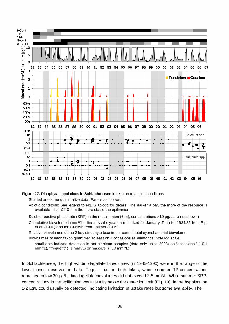
38

Figure 27. Dinophyta populations in Schlachtensee in relation to abiotic conditions Shaded areas: no quantitative data. Panels as follows: Abiotic conditons: See legend to Fig. S abiotic for details. The darker a bar, the more of the resource is

available – for ΔT 0-4 m the more stable the epilimnion

Soluble reactive phosphate (SRP) in the metalimnion (6 m); concentrations >10 µg/L are not shown) Cumulative biovolume in mm³/L – linear scale; years are marked for January. Data for 1984/85 from Ripl

et al. (1990) and for 1995/96 from Fastner (1999). Relative biovolumes of the 2 key dinophyte taxa in per cent of total cyanobacterial biovolume Biovolumes of each taxon quantified at least on 4 occasions as diamonds; note log scale; small dots indicate detection in net plankton samples (data only up to 2003) as “occasional” (~0.1

mm³/L), “frequent” (~1 mm³/L) or“massive” (~10 mm³/L)

In Schlachtensee, the highest dinoflagellate biovolumes (in 1985-1990) were in the range of the lowest ones observed in Lake Tegel – i.e. in both lakes, when summer TP-concentrations remained below 30 µg/L, dinoflagellate biovolumes did not exceed 3-5 mm³/L. While summer SRP-concentrations in the epilimnion were usually below the detection limit (Fig. 19), in the hypolimnion 1-2 µg/L could usually be detected, indicating limitation of uptake rates but some availablity. The

NO3-NTPSRPSecchi ΔT 0-4 m

Ceratium spp.

0,0010,01

0,11

10100

Peridinium spp.

0,0010,01

0,11

10100

82 83 84 85 86 87 88 89 90 91 92 93 94 95 96 97 98 99 00 01 02 03 04 05 06

0%20%40%60%80%

100%

82 83 84 85 86 87 88 89 90 91 92 93 94 95 96 97 98 99 00 01 02 03 04 05 06

0

1

2

3

Bio

volu

me

[mm

³/L]

Peridinium Ceratium

0

5

10

82 83 84 85 86 87 88 89 90 91 92 93 94 95 96 97 98 99 00 01 02 03 04 05 06 07SRP

6m [µ

g/L]


Ceratium spp.

0,0010,01

0,11

10100

Peridinium spp.

0,0010,01

0,11

10100

82 83 84 85 86 87 88 89 90 91 92 93 94 95 96 97 98 99 00 01 02 03 04 05 06

Ceratium spp.

0,0010,01

0,11

10100

Peridinium spp.

0,0010,01

0,11

10100

82 83 84 85 86 87 88 89 90 91 92 93 94 95 96 97 98 99 00 01 02 03 04 05 06

Ceratium spp.

0,0010,01

0,11

10100

Ceratium spp.

0,0010,01

0,11

10100

Peridinium spp.

0,0010,01

0,11

10100

82 83 84 85 86 87 88 89 90 91 92 93 94 95 96 97 98 99 00 01 02 03 04 05 06

0%20%40%60%80%

100%

82 83 84 85 86 87 88 89 90 91 92 93 94 95 96 97 98 99 00 01 02 03 04 05 06

0

1

2

3

Bio

volu

me

[mm

³/L]

Peridinium Ceratium

0%20%40%60%80%

100%

82 83 84 85 86 87 88 89 90 91 92 93 94 95 96 97 98 99 00 01 02 03 04 05 06

0

1

2

3

Bio

volu

me

[mm

³/L]

Peridinium Ceratium

0%20%40%60%80%

100%

82 83 84 85 86 87 88 89 90 91 92 93 94 95 96 97 98 99 00 01 02 03 04 05 060%

20%40%60%80%

100%

82 83 84 85 86 87 88 89 90 91 92 93 94 95 96 97 98 99 00 01 02 03 04 05 06

0

1

2

3

Bio

volu

me

[mm

³/L]

Peridinium Ceratium

0

5

10

82 83 84 85 86 87 88 89 90 91 92 93 94 95 96 97 98 99 00 01 02 03 04 05 06 07SRP

6m [µ

g/L]

39

Figure 28. Dinophyta populations in Lake Tegel in relation to abiotic conditions Shaded areas: no quantitative data. Panels as follows: Abiotic conditons: See legend to Fig. T abiotic for details. The darker a bar, the more of the resource is


Soluble reactive phosphate (SRP) in the metalimnion (11 m); concentrations >10 µg/L are not shown) Cumulative biovolume in mm³/L – linear scale (levels >20 mm³/L not shown); years are marked for

January. Data for 1995/96 from Fastner (1999) Relative biovolumes of the 6 key dinophyte taxa in per cent of total dinophyte biovolume Biovolumes of each taxon quantified at least on 4 occasions as diamonds; note log scale; small dots indicate detection in net plankton samples (data only up to 2003) as “occasional” (~0.1

mm³/L), “frequent” (~1 mm³/L) or“massive” (~10 mm³/L)

dinoflagellate maximum in September 1987 coincided with an SRP peak of 43 µg/L in the hypolimnion (Fig. 27).

In Lake Tegel biovolumes were highest while epilimnion TP-concentrations were still mostly above 50 µg/L, i.e. in the early 1990s and again during re-eutrophication in the late 1990’s until 2003 (Fig. 28 and Fig. 19). Ceratium biovolumes also reflect the concentrations of soluble reactive phosphorus (SRP) in the meta- and hypolimnion (shown for 11 m in Fig. 28): their pronounced decline in 1994 coincided with the summer hypolimnetic minimum of <5 µg/L.


Ceratium spp.

0,0010,010,1

110

100

Peridinium spp.

0,0010,01

0,11

10100

84 85 86 87 88 89 90 91 92 93 94 95 96 97 98 99 00 01 02 03 04 05 06

0%20%40%60%80%

100%

87 88 89 90 91 92 93 94 95 96 97 98 99 00 01 02 03 04 05 06

0

5

10

15

20

Bio

volu

me

[mm

³/L]

39 31 46

0

5

10

84 85 86 87 88 89 90 91 92 93 94 95 96 97 98 99 00 01 02 03 04 05 06SRP

11m

[µg/

L]


Ceratium spp.

0,0010,010,1

110

100

Peridinium spp.

0,0010,01

0,11

10100

84 85 86 87 88 89 90 91 92 93 94 95 96 97 98 99 00 01 02 03 04 05 06

0%20%40%60%80%

100%

87 88 89 90 91 92 93 94 95 96 97 98 99 00 01 02 03 04 05 06

0

5

10

15

20

Bio

volu

me

[mm

³/L]

39 31 46

Ceratium spp.

0,0010,010,1

110

100

Peridinium spp.

0,0010,01

0,11

10100

84 85 86 87 88 89 90 91 92 93 94 95 96 97 98 99 00 01 02 03 04 05 06

Ceratium spp.

0,0010,010,1

110

100

Peridinium spp.

0,0010,01

0,11

10100

84 85 86 87 88 89 90 91 92 93 94 95 96 97 98 99 00 01 02 03 04 05 06

0%20%40%60%80%

100%

87 88 89 90 91 92 93 94 95 96 97 98 99 00 01 02 03 04 05 06

0

5

10

15

20

Bio

volu

me

[mm

³/L]

39 31 46

0%20%40%60%80%

100%

87 88 89 90 91 92 93 94 95 96 97 98 99 00 01 02 03 04 05 06

0

5

10

15

20

Bio

volu

me

[mm

³/L]

0%20%40%60%80%

100%

87 88 89 90 91 92 93 94 95 96 97 98 99 00 01 02 03 04 05 060%

20%40%60%80%

100%

87 88 89 90 91 92 93 94 95 96 97 98 99 00 01 02 03 04 05 06

0

5

10

15

20

Bio

volu

me

[mm

³/L]

39 31 46

0

5

10

84 85 86 87 88 89 90 91 92 93 94 95 96 97 98 99 00 01 02 03 04 05 06SRP

11m

[µg/

L]

40

0

3

6

9

12

frequ

ency

bio

volu

me

Cer

>Mic

Cer / Mic>1Cer / Mic>2

0

4

8

12

16

0-<1 1-<3 3-<6 6-<8 8-<9 9-<10 10->11

11-<12

>=12

Δ T 0-11 m [°C]

frequ

ency

Mic > 1 mm³/LCer > 1 mm³/L

0

5

10

15

20

14/15 13/12 11 10 9 8 7 6/5

depth of thermocline [m]

frequ

ency


0

3

6

9

12

frequ

ency

bio

volu

me

Cer

>Mic


0

3

6

9

12

frequ

ency

bio

volu

me

Cer

>Mic


0

4

8

12

16

0-<1 1-<3 3-<6 6-<8 8-<9 9-<10 10->11

11-<12

>=12

Δ T 0-11 m [°C]

frequ

ency


0

5

10

15

20

14/15 13/12 11 10 9 8 7 6/5

depth of thermocline [m]

frequ

ency


Figure 29. Ceratium versus Microcystis in Lake Tegel in relation to the temperature gradient between 0 and 11 m depth and the depth of the thermocline

Panels: 1. Ceratium / Microcystis biovolume ratios > 1 or > 2 (see legend) 2. Frequencies of each taxon in relation to vertical temperature gradients 3. Frequencies of each taxon in relation to the depth of the thermocline

These patterns indicate that SRP in the hypolimnion may support dinoflagellate popu-lation growth if thermal stratification is sufficiently stable so that they can efficiently access it through vertical migration. Gene-rally, vertical migration was not investigated, but biovolume data with vertical resolution available for one year from Lake Tegel show pronounced gradients of Ceratium spp. over depth on days with stable thermal gradients (Löhr, pers. com.), reflecting Ceratium’s active vertical positioning. How-ever, the analysis of Ceratium biovolumes in relation to stratification stability in Lake Tegel reveals a competitive ad-vantage for Ceratium at times of stable stratification: Relative shares of summer phytoplankton biovolumes shifted from cyanobacterial dominance to dinoflagellate (i.e. Ceratium) dominance a year after aerator-induced mixing was reduced, so that the lake developed a much more stable stratification (reflected by pronounced vertical temperature gra-

dients; Fig. 19). While Reynolds et al. (2002) assign Ceratium spp. and Microcystis spp. to the same habitat, the data from Lake Tegel indicate that in a more turbulent environment Microcystis spp. have a competitive advantage over Ceratium spp.: We used the temperature difference be-tween 0 and 11 m as an indicator for the turbulence that Ceratium would need to overcome when migrating to the hypolimnion for uptake of dissolved phosphorus. The results show that Ceratium outcompeted Microcystis (as defined by volume ratio of >1) when thermal stratification was usually very stable, with ΔT 0-11 m of at least 6 °C or more (Fig. 29 upper panel), and for 18 of the 19

41

samples with very high biovolume ratios of Ceratium to Microcysts (i.e. Cer/Mic >10) ΔT 0-11 m was higher than 5 °C. Also, Microcystis spp. occurred more frequently at biovolumes > 1 mm³/L if vertical temperature gradients amounted to <6 °C, while Ceratium frequencies peaked at gradients of 6-10 °C (Fig. 29, middle panel). Both species rarely reached biovolumes >1 mm³/L at the very high end of the ΔT range because this condition usually occurred in early summer, before either species had enough time to build up a large population. Their frequency of occurrence across categories of the depth of the thermocline show a similar pattern (Fig. 29, lower panel): Ceratium spp. reached biovolumes >1 mm³/L most often if the thermocline was at 8-10 m and rarely if it was deeper, while Microcystis spp. more often maintained a population of >1 mm³/L even at almost total overturn (mixing depths of 14-15 m).

In summary, in both lakes phosphorus concentrations determined the population levels of dinoflagellates, with their largest populations observed in the transition phase from hypertrophic to eutrophic, when they were able to outcompete cyanobacteria in some years. In Lake Tegel, the stability of thermal stratification – strongly affected by aerator management – is a further factor affecting dinoflagellate growth, particularly that of Ceratium in competition against Microcystis.

Chrysophyta Chrysophyta responded strongly to restoration: both lakes did not harbour Chrysophyta in numbers sufficiently high for enumeration during their hypertrophic phase, though some species occurred occasionally in the seston sampled with the plankton net. Among the taxa recorded in net samples and enumerated, only Dinobryon spp. continued to occur regularly in both lakes, once they had appeared (Fig. 30 and 31). In Schlachtensee, they constituted the dominant early summer phytoplankton in 1987, 1995 and 2002, while in Lake Tegel their share of total phytoplankton biomass was marginal throughout the study period (1994-2005; see Fig. 20 and 21).

• In Schlachtensee, Chrysophyta first became quantitatively relevant with Dinobryon spp. in summer 1984, the first year in which pH remained below 8.5. It was followed by Mallomonas spp. as species with winter maximum in early 1986 and by Uroglena spp. as summer species in 1987. Uroglena spp. often – but not always – co-occurred with Dinobryon spp.. Only three samples (summer 1992 and 1995) contained Synura spp. with a frequency sufficient for quantification, attaining biovolumes between 0.1 and 1 mm³/L (Fig 30).

• In Lake Tegel, Dinobryon spp. were recorded in spring and early summer amounts sufficient for quantification, but their biovolume never exceeded 1 mm³/L (Fig. 31). They first appeared in 1994, at pH below 8.5. Mallomonas spp. were never observed in samples from Lake Tegel, Synura spp. were recorded once in the net plankton at levels classified as “frequent” and Uroglena spp. were recorded once in July in net plankton as “massive”. Thus the only Chrysophyta of repeated quantitative relevance in Lake Tegel was Dinobryon spp.

In both lakes, Chrysophyte biovolumes show little direct response to patterns of the concentrations of nutrients, turbulence or Secchi-Disc readings. However, none of the quantitative records for Chrysophytes are from the eutrophic years while pH still ranged up to 10.5 in Schlachtensee (before 1982; data not shown) and up to 9 in Lake Tegel. Thus, the data from both lakes confirm the general understanding of hydrogen ion concentration (pH) as a key abiotic parameter determining Chrysophyte species occurrence. In both lakes reduced pH is a consequence of re-

42

Figure 30. Chrysophyta populations in Schlachtensee in relation to abiotic conditions Shaded areas: no quantitative data. Panels as follows: Abiotic conditons: See legend to Fig. S abiotic for details. The darker a bar, the more of the resource is


Mean pH in the epilimnion (0-4 m) Cumulative biovolume in mm³/L – linear scale (levels >1.5 mm³/L not shown); years are marked for

January. Data for 1984/85 from Ripl et al. (1990) and for 1995/96 from Fastner (1999). Relative biovolumes of the 6 key chryosphyte taxa in per cent of total chrysophyte biovolume Biovolumes of each taxon quantified at least on 4 occasions (diamonds; note log scale; small dots indicate detection in net plankton samples (data only up to 2003) as “occasional” (0.01

mm³/L), “frequent” (0.1 mm³/L) or“massive” (1 mm³/L)

Uroglena spp.

0,0010,010,1

110

100

Dinobryon spp.

0,0010,010,1

110

100

Synura spp.

0,0010,010,1

110

100

Mallomonas spp.

0,0010,010,1

110

100

82 83 84 85 86 87 88 89 90 91 92 93 94 95 96 97 98 99 00 01 02 03 04 05 06

6,57,58,59,5

pHNO3-NTPSRPSecchi ΔT 0-4 m

0

0,5

1

1,5

Biov

olum

e [m

m³/L

]

MallomonasSynuraUroglenaDinobryon

0%

20%

40%

60%

80%

100%

82 83 84 85 86 87 88 89 90 91 92 93 94 95 96 97 98 99 00 01 02 03 04 05 06

Uroglena spp.

0,0010,010,1

110

100

Dinobryon spp.

0,0010,010,1

110

100

Synura spp.

0,0010,010,1

110

100

Mallomonas spp.

0,0010,010,1

110

100

82 83 84 85 86 87 88 89 90 91 92 93 94 95 96 97 98 99 00 01 02 03 04 05 06

Uroglena spp.

0,0010,010,1

110

100

Dinobryon spp.

0,0010,010,1

110

100

Synura spp.

0,0010,010,1

110

100

Mallomonas spp.

0,0010,010,1

110

100

82 83 84 85 86 87 88 89 90 91 92 93 94 95 96 97 98 99 00 01 02 03 04 05 06

6,57,58,59,5

pH

6,57,58,59,5

pHNO3-NTPSRPSecchi ΔT 0-4 m

0

0,5

1

1,5

Biov

olum

e [m

m³/L

]


0%

20%

40%

60%

80%

100%

82 83 84 85 86 87 88 89 90 91 92 93 94 95 96 97 98 99 00 01 02 03 04 05 06

0

0,5

1

1,5

Biov

olum

e [m

m³/L

]


0%

20%

40%

60%

80%

100%

82 83 84 85 86 87 88 89 90 91 92 93 94 95 96 97 98 99 00 01 02 03 04 05 06

0

0,5

1

1,5

Biov

olum

e [m

m³/L

]


0%

20%

40%

60%

80%

100%

82 83 84 85 86 87 88 89 90 91 92 93 94 95 96 97 98 99 00 01 02 03 04 05 06

0

0,5

1

1,5

Biov

olum

e [m

m³/L

]


0

0,5

1

1,5

Biov

olum

e [m

m³/L

]


0%

20%

40%

60%

80%

100%

82 83 84 85 86 87 88 89 90 91 92 93 94 95 96 97 98 99 00 01 02 03 04 05 06

43

Figure 31. Chrysophyta populations in Lake Tegel in relation to abiotic conditions Shaded areas: no quantitative data. Panels as follows: Abiotic conditons: See legend to Fig. S abiotic for details. The darker a bar, the more of the resource is


Mean pH in the epilimnion (0-8 m) Cumulative biovolume in mm³/L – linear scale; years are marked for January. Data for 1995/96 from

Fastner (1999). Relative biovolumes of the 6 key chryosphyte taxa in per cent of total cyanobacterial biovolume Biovolumes of each taxon quantified at least on 4 occasions (diamonds; note log scale; small dots indicate detection in net plankton samples (data only up to 2003) as “occasional” (0.01

mm³/L), “frequent” (0.1 mm³/L) or“massive” (1 mm³/L)

duced primary production through oligotrophication. Furthermore, the data indicate a gradient in pH-ranges favouring the three species, with Uroglena spp. being most tolerant of higher pH, followed first by Dinobryon spp. and then by Mallomonas spp. (Fig. 32).

Uroglena spp. occurred in Schlachtensee chiefly during the initial phase of pronounced trophic recovery between 1987 and 1997, when pH-levels were frequently still well above 8 (Fig. 32, lower panel). While their highest biovolumes (up to 15 mm³/L at pH 8.45 in 1988) were registered at pH >8, Uroglena spp. occurred most frequently at pH 7.5 – 7.7. During their maximum population size in 1987, Uroglena spp. were the likely cause of a pronounced odour event attributed to 2-4-heptadienal and 2-4 decadienals found in high concentrations (Chorus et al. 1992).

Dinobryon spp. show a similar response to pH in both lakes, with biomass maxima in the pH range of 7.5 – 8.3 and still frequent occurrence, though at lower levels, at pH up to 8.3 in Lake Tegel and pH 8.7 in Schlachtensee (Fig. 32, lower panel).

Mallomonas spp. occurred in Schlachtensee most frequently at lower pH, i.e. between 7 and 7.7 (Fig. 30), but the causality for this remains unclear, as pH is also generally lower in winter when photosynthetic activity is low, and this taxon typically developed its maxima in winter or late autumn.


6,57,58,5

84 84 85 87 88 89 90 91 92 93 94 95 96 97 98 99 00 01 02 03 04 05 06

pH

Dinobryon spp.

0,0010,01

0,11

10100

84 85 86 87 88 89 90 91 92 93 94 95 96 97 98 99 00 01 02 03 04 05 06

0

0,5

1B

iovo

lum

e [m

m³/L

]

Dinobryon spp.


6,57,58,5

84 84 85 87 88 89 90 91 92 93 94 95 96 97 98 99 00 01 02 03 04 05 06

pHNO3-N TPSRPSecchiΔT 0-8 m

6,57,58,5

84 84 85 87 88 89 90 91 92 93 94 95 96 97 98 99 00 01 02 03 04 05 06

pH

6,57,58,5

84 84 85 87 88 89 90 91 92 93 94 95 96 97 98 99 00 01 02 03 04 05 06

pH

Dinobryon spp.

0,0010,01

0,11

10100

84 85 86 87 88 89 90 91 92 93 94 95 96 97 98 99 00 01 02 03 04 05 06

0

0,5

1B

iovo

lum

e [m

m³/L

]

Dinobryon spp.

Dinobryon spp.

0,0010,01

0,11

10100

84 85 86 87 88 89 90 91 92 93 94 95 96 97 98 99 00 01 02 03 04 05 06

0

0,5

1B

iovo

lum

e [m

m³/L

]

Dinobryon spp.

44

Figure 32. Frequency of occur-rence and biovolumes of Chry-sophytes in relation to pH Upper panel: Frequency of occurrence in Schlachtensee

Lower panel: Biovolumes in Schlachtensee and Lake Tegel

Bacillariophyta (diatoms)

The total diatom biovolume of both lakes reflects TP-concentrations only slightly – clearly less than observed for most of the other phytoplankton groups:

• For Schlachtensee, the clearest reflection of oligotrophication is that no diatom maxima of more than 5 mm³/L biovolume have been recorded since 1995 (Fig. 33). However, diatom maxima were highest in spring of the late 1980’s, when TP-concentrations had already dropped to usually 30 µg/L or less, even during winter overturn (Fig. 19). Also, while the TP maxima of 50 µg/L in spring 1987 and January 1990 coincide with diatom maxima, a similar TP-peak in early 1996 does not.

• For Lake Tegel, the oligotrophication response of the diatoms is yet weaker: somewhat lower summer maxima were recorded in the years with summer TP levels below 30 µg/L, i.e. 1994 – 1996 and 2003 – 2006 (Fig. 34). However, during winter overturn and spring the

024

68

1012

1416

< 7.5 7.5 -<7.7

7.7 -<7.9

7.9 -<8.1

8.1 -<8.3

8.8 -<8.5

8.5 -<8,7

pH categories

Fre

quen

cy o

f occ

urre

nce Dinobryon

MallomonasUroglena

0

1

2

3

4

5

6,50 7,00 7,50 8,00 8,50 9,00pH

Bio

volu

me

[mm

³/L]

Dinobryon Lake TDinobryon Lake SMallomonas Lake SUroglena Lake S

8.45/15

6.5 7.0 7.5 8.0 8.5 pH

7.5 pH

45

TP concentrations in Lake Tegel are still much higher (>100 µg/L; Fig. 19) than in Schlachtensee, and thus spring diatom blooms are not P-limited.

Silicate limitation could be key to determining diatom biomass, and published experimental data show that concentrations of dissolved silicate would start limiting uptake rates only if they drop well below 0.5 mg/L of Si. This derives from half-saturation constants for the uptake of silicate (Si) which are in the range of 0.05 for many diatoms (Asterionella formosa, Fragilaria crotonensis and Diatoma elongatum; Tilman et al. 1981) to 0.122 (Synedra ulna; Tilman et al. 1981). Data for silicate are available for 1994-1999 for Lake Tegel and from 1996-1999 for Schlachtensee. In both lakes, concentrations of dissolved and total Si (data not shown) were well above 1 mg/L for most of the year, thus well above limiting levels. In Lake Tegel, summer minima of dissolved silicate did not drop below 0.5 mg/L Si and rarely below 1 mg/L during the five years monitored, indicating that silicate is unlikely to limit diatom growth. In Schlachtensee, minima of 0.07 – 0.22 mg/L dissolved Si recorded in late spring of 1998 indicate that at times of diatom biovolume maxima, silicate concentratons may start limiting uptake rates, but do not exert severe control of population sizes. As we can also exclude nitrogen limitation as important factor for phytoplankton growth in both lakes, mixing and stratification remain as likely candidates determining diatom growth. The very variable taxonomic composition of diatom populations in both lakes supports this assumption:

Asteriionella formosa was the most frequently occurring diatom species in both lakes, sometimes dominant, particularly in early spring or winter. This is in line with the restoration response of the species in both Berlin lakes: Overall, A. formosa shows a slight tendency of population maxima decline as oligotrophication proceeds, although this does not clearly relate to phosphorus levels (Fig. 33 and 34).

In Schlachtensee, summer populations of A. formosa were rare and almost always minor. Time patterns in relation to those for the temperature difference between 0 and 4 m depth (ΔT 0-4 m) show that the populations decline usually well before ΔT 0-4 m starts becoming pronounced (Fig. 33). In a few summers (1986, 1987, 1998, 2002), A. formosa could reach or maintain populations of 0.1 – 1 mm³/L biovolume even in situations with some epilimnetic temperature gradient, but the populations declined as ΔT 0-4 m increased or immediately after its peak.

In Lake Tegel, A. formosa was more frequent but shows a similar time pattern in relation to seasonal temperature gradients (ΔT 0-8 m; Fig. 34). Lake Tegel also supported some small and brief early summer populations of A. formosa, e.g. in June 1996, May 2001 and early July 2006. These tend to reflect phases of reduced stratifycation stability which are typical for this larger, more wind-exposed lake, and once ΔT 0-8 m increased, A. formosa rapidly declined. Apparently, although the star-shaped colonies of this species provide some form resistance against losses through sedimentation, this is not enough once the water-body becomes very stable.

Fragilaria spp. (i.e. colony-forming species, often chiefly F. crotonensis) were the other very frequent group in both lakes. They typically occurred in mid- to late summer, usually during phases with low epilimnetic temperature gradients. This is particularly conspicuous in the Schlachtensee data: “Fragilaria-summers” were typically those in which ΔT 0-4 m remained low, rarely exceeding < 4 °C (Fig. 33). In Lake Tegel, in years with more pronounced

46

epilimnetic temperature gradients, Fragilaria spp. populations reached surprisingly high maxima. Although maxima coincided tightly with peaks of ΔT 0-8 m above 5°C, they then declined steeply (1992-1996 and 1998; Fig. 34). These patterns indicate that Fragilaria spp. populations can grow in spite of little turbulence to keep them in suspension. Their cells join to form ribbon-like combs which render them both more readily entrainable by turbulence and more resistant against sinking than individual cells (see discussion in Reynolds 1997).

Interestingly, Fragilaria spp. started becoming relevant in Schlachtensee only in 1986, when the lake was already close to mesotrophic.

Fragilaria acus (formerly Synedra acus) was common in both lakes during most years. In Schlachtensee, it formed early spring maxima in a number of years (Fig. 33) and in Lake Tegel in every year for which quantitative data are available (Fig. 34). These maxima always declined sharply when thermal gradients began to appear in the epilimnion, although small numbers were still collected in the plankton net, indicating that an inoculum remained present that could quickly seed population growth if conditions turned favourable. In fact, the only significant mid-summer population recorded in Schlachtensee (15th July 1998) coincided with a short phase of unusually pronounced summer epilimnetic mixing, indicated by equal temperatures at 0 and 4 m depth. This species occurs as single cells, not joined to form ribbon-like combs, thus needing more turbulence to remain in suspension than the colony-forming species of the genus Fragilaria.

In Schlachtensee, Fragilaria acus was not recorded since 1999, not even in the samples enriched with the plankton net (collected regularly until 2003), while in Lake Tegel, it continued to form populations until the end of the study in 2006. Whether or not its disappearance from Schlachtensee reflects this lake’s more pronounced trophic recovery remains unclear.

Tabellaria fenestrata, a further large pennate diatom with cells joining to star-shaped colonies (similar to Asterionella formosa, though with larger, stronger cells), surprisingly occurred only in Schlachtensee, and there only from 1987 to 1994. It formed substantial and extended populations in 1988 and 1990, with a sharp maximum in early September 1988 reflecting increased epilimnetic mixing. The population abruptly disappeared later in September when the epilimnion regained stability (with temperature differences between 0 and 4 m back up to almost 3 °C; Fig. 33).

Diatoma spp. (often primarily D. elongatum) – a pennate diatom joining to zig-zag shaped bands – occurred in both lakes almost in all years, at least in numbers sufficient for recording in plankton net samples (Fig. 33 and 34). Numbers sufficient for enumeration occurred periodically in both lakes – in Schlachtensee particularly in the hypertrophic phase and again in the late 1980’s. In both lakes, populations became quantitatively significant when epilimnetic temperature gradients were absent or weak – in Schlachtensee during spring, and in Lake Tegel also during some summers, but clearly restricted to phases of low or declining ΔT 0-8 m (e.g. 1996, 1997, 2004).

Interestingly, in Lake Tegel, Diatoma spp. became quantitatively relevant only in 1992. This does not reflect trophic recovery, as TP-concentrations were still well above 50 µg/L for almost all of that year. Maxima were not limited to spring, but also occurred in mid- and late

47

summer, i.e. in 1993-1995, 1997-199, 2001, 2004-2005 (Fig. 34). Almost all of these coincide with pronounced thermal gradients in the epilimnion. This is in line with the change in aerator management towards inducing less artificial mixing – 1992 was the first year in which thermal stratification was substantially more stable. This suggests Diatoma’s colony morphology to function as effective form resitance against sedimentation in Lake Tegel.

Nitzschia spp. (often including N. acicularis, N. actinastroides) – a small, single-celled needle-shaped pennate diatom, was frequent in Lake Tegel, forming populations sufficiently large for enumeration in most years of the study (Fig. 34), while in Schlachtensee, net plankton samples always contained some Nitzschia cells, but sizable populations were recorded only occasionally – chiefly in 1982 and 1983 while the lake was still hypertrophic (Fig. 33). Maxima typically occurred in spring, and the few low-level late summer populations in Lake Tegel coincided with epilimnetic mixing.

Centric diatoms were recorded and quantified as bulk group differentiated not taxonomically, but rather by three size classes, i.e. with cell diameters of < 8 µm, 8-15 µm and > 15 µm, however excluding the filamentous genus Aulacoseira. These Centrales also chiefly occurred when the lakes or their epilimnions were well mixed.

Exceptions in Schlachtensee with populations of Centrales while ΔT > 4 °C were recorded in May 1984 and 1985 (data by Wesseler; no differentiation by size groups available), as well as in May and July of 2004 and 2006 (consisting only of Centrales in the size groups <8 and 8-15 µm; Fig. 33).

Exceptions in Lake Tegel are June 1997, where the Centrales peaked during stable conditions with a temperature gradient of 4 °C between 0 and 8 m depth. These were either medium-sized or small; i.e. the size group 8-15 µm contributed a biovolume of 7 mm³/L and those < 8 µm reached 6 mm³/L. Small cells have a lower sinking velocity than large ones, which were not recorded on this sampling occasion. Substantial populations of large Centrales (diameter > 15 µm) were scarcely recorded while the epilimnion was very stable (Δ T > 5-6 °C), e.g. in May 2001, followed by a population decline (Fig. 34).

Aulacoseira spp. (formerly Melosira spp.; often including major shares of A. granulata) occurred very regularly in both lakes, though in Schlachtensee never in numbers sufficient for quantification, and in plankton-net enriched samples they were rarely detected more than occasionally (Fig. 33). In contrast, in the more turbulent Lake Tegel, these large filaments formed quite substantial populations in every year, usually with maxima in late summer and autumn, and sometimes also in spring. Aulacoseira populations typically increased steeply as soon as thermal gradients within the epilimnion started to decrease (Fig. 34). Even transient spurts of mid-summer population growth of Aulacoseira spp. coincide with brief phases of epilimnetic mixing, e.g. in 1990, 1994-1995. Thus it appears that Lake Tegel’s more turbulent water body was more favourable for Aulacoseira spp. to outcompete other diatoms than was Schlachtensee’s less turbulent environment.

48

Figure 33. Bacillariophyta populations in Schlachtensee in relation to abiotic conditions Shaded areas: no quantitative data. Panels as follows: Abiotic conditons: See legend to Fig. 19 for details. The darker a bar, the more of the resource is available – for ΔT

0-4 m the more stable the epilimnion Cumulative biovolume in mm³/L – linear scale (levels >5 mm³/L not shown); years are marked for Jan. Data

1984/1985 from Ripl et al. (1990; for 1985 summer pennales maximum is not shown due to lack of further taxonomic resolution); data for 1995/96 from Fastner (1999).

Relative biovolumes of the 7 key taxa and of the Centrales (sum of all size groups) in per cent of total diatom biovolume

Biovolumes of each taxon quantified at least on 4 occasions (diamonds; note log scale; shaded areas: no quantitative data); small dots indicate detection in net plankton samples (data only up to 2003) as “occasional” (0.01 mm³/L), “frequent” (0.1 mm³/L) or“massive” (1 mm³/L); red curves show ΔT 0-4 m


Diatoma spp.

0,0010,010,1

110

100

Fragilaria spp.

0,0010,010,1

110

100

Nitzschia spp.

0,0010,010,1

110

100

Aulacoseira spp.

0,0010,010,1

110

100

Fragilaria acus / syn. Synedra acus

0,0010,010,1

110

100

Centrales (all sizes, non-filamentous)

0,0010,010,1

110

100

80 81 82 83 84 85 86 87 88 89 90 91 92 93 94 95 96 97 98 99 00 01 02 03 04 05 06

Tabellaria fenestrata

0,0010,010,1

110

100

Asterionella formosa

0,0010,010,1

110

100

0%20%40%60%80%

100%

82 83 84 85 86 87 88 89 90 91 92 93 94 95 96 97 98 99 00 01 02 03 04 05 06

0

1

2

3

4

5

Biov

olum

e [m

m³/L

] Nitzschia AsterionellaFragilaria spp. Synedra/Fragilaria acusDiatoma TabellariaCentrales Pennales (1984-86)


Diatoma spp.

0,0010,010,1

110

100

Fragilaria spp.

0,0010,010,1

110

100

Nitzschia spp.

0,0010,010,1

110

100

Aulacoseira spp.

0,0010,010,1

110

100Aulacoseira spp.

0,0010,010,1

110

100

Fragilaria acus / syn. Synedra acus

0,0010,010,1

110

100


0,0010,010,1

110

100

80 81 82 83 84 85 86 87 88 89 90 91 92 93 94 95 96 97 98 99 00 01 02 03 04 05 06

Tabellaria fenestrata

0,0010,010,1

110

100


0,0010,010,1

110

100

0%20%40%60%80%

100%

82 83 84 85 86 87 88 89 90 91 92 93 94 95 96 97 98 99 00 01 02 03 04 05 06

0

1

2

3

4

5

Biov

olum

e [m

m³/L

] Nitzschia AsterionellaFragilaria spp. Synedra/Fragilaria acusDiatoma TabellariaCentrales Pennales (1984-86)

49

Figure 34. Bacillariophyta populations in Lake Tegel in relation to abiotic conditions Shaded areas: no quantitative data. Panels as follows: Abiotic conditons: See legend to Fig. 19 for details. The darker a bar, the more of the resource is

available – for ΔT 0-8 m the more stable the epilimnion Cumulative biovolume in mm³/L – linear scale (levels >5 mm³/L not shown); years are marked for

January. Data for 1995/96 are from Fastner (1999). Relative biovolumes of the 7 key taxa and of the Centrales (sum of all size groups) in per cent of total

diatom biovolume Biovolumes of each taxon quantified at least on 4 occasions (diamonds; note log scale; shaded areas:

no quantitative data); small dots indicate detection in net plankton samples (data only up to 2003) as “occasional” (0.01 mm³/L), “frequent” (0.1 mm³/L) or“massive” (1 mm³/L); red curves show ΔT 0-8 m

0

5

10

15B

iovo

lum

e [m

m³L

] Nitschia Asterionella Fragilaria spp.Synedra/Fragilaria acus Diatoma Aulacoseiracentric diatoms

0%20%40%60%80%

100%

87 88 89 90 91 92 93 94 95 96 97 98 99 00 01 02 03 04 05 06

NO 3-N TPSRPSecchi?T 0-8 m


0,0010,010,1

110

100

84 85 86 87 88 89 90 91 92 93 94 95 96 97 98 99 00 01 02 03 04 05 06

Fragilaria spp.0,0010,010,1

110

100

Diatoma spp.

0,0010,010,1

110

100


0,0010,010,1

110

100

Fragilaria acus/ syn. Synedra acus0,0010,010,1

110

100

Nitzschia spp.

0,0010,010,1

110

100

Aulacoseira spp.

0,0010,010,1

110

100

0

5

10

15B

iovo

lum

e [m

m³L


0%20%40%60%80%

100%

87 88 89 90 91 92 93 94 95 96 97 98 99 00 01 02 03 04 05 06

0

5

10

15B

iovo

lum

e [m

m³L


0

5

10

15B

iovo

lum

e [m

m³L


0%20%40%60%80%

100%

87 88 89 90 91 92 93 94 95 96 97 98 99 00 01 02 03 04 05 06

NO 3-N TPSRPSecchi?T 0-8 m


0,0010,010,1

110

100

84 85 86 87 88 89 90 91 92 93 94 95 96 97 98 99 00 01 02 03 04 05 06


0,0010,010,1

110

100

84 85 86 87 88 89 90 91 92 93 94 95 96 97 98 99 00 01 02 03 04 05 06

Fragilaria spp.0,0010,010,1

110

100

Diatoma spp.

0,0010,010,1

110

100


0,0010,010,1

110

100Asterionella formosa

0,0010,010,1

110

100

Fragilaria acus/ syn. Synedra acus0,0010,010,1

110

100

Nitzschia spp.

0,0010,010,1

110

100Nitzschia spp.

0,0010,010,1

110

100

Aulacoseira spp.

0,0010,010,1

110

100Aulacoseira spp.

0,0010,010,1

110

100

50

In summary, for both lakes some overall decline of diatom biovolume can be attributed to trophic recovery. Both the changes over time in the occurrence of taxa and the differences of diatom species composition between both lakes, however, largely reflect the intensity of mixing within the epilimnion or the whole water-body: the time patterns of occurrence of most diatom taxa correspond to time patterns of temperature gradients between the surface and the bottom of the epilimnion (ΔT 0-4 m for Schlachtensee and ΔT 0-8 m for Lake Tegel.), with some taxa or size groups responding to a lack of turbulence more sensitively than others. While this also applies to Tabellaria spp., we found no hypothesis to explain their appearance for a 7-year period from1987-1994 only in Schlachtensee.

Cryptophyta The Cryptophyta identified to the species level included the large Cryptomonas rostratiformis and Cryptomonas ovata, the rather small Chroomonas nordstedtii, and the minute Rhodomonas lens. Additionally, Gervais (1991) identified Cryptomonas phaseolus as species growing exclusively in the metalimnetic layer with oxygen concentrations <1 mg/L. Several further Cryptomonas morphotypes were apparent in the samples. However, species characteristics of these flagellates were not sufficiently stable for distinction during enumeration, so the Cryptophytes were counted by size categories, the biovolume calculated for each category and the total sum of their biovolumes shown as Cryptomonas spp., distinguishing only Rhodomonas lens from the rest (Fig. 35 and 36). Furthermore, Cryptophyta are very poorly captured with phytoplankton nets, so Fig. 35 and 36 show no net plankton data. In both lakes, Cryptophyta occurred in almost every sample. Their epilimnetic biovolume maxima reached 4 mm³/L in Lake Tegel and 5 mm³/L in Schlachtensee. Also, in each lake, time patterns of occurrence were roughly similar for Rhodomonas lens and the other Cryptophyta, and a Spearman rank correlation between the biovolumes of both groups is significant on the 0.05 level for Schlachtensee and on the 0.01 level for Lake Tegel. Nonetheless, the relative biomass share of R. lens varies substantially in relation to the other Cryptophyta (Fig. 35 and 36), and this ratio shows no seasonal patterns or a relationship to trophic change.

Seasonality of Cryptophyta occurrence shows regular patterns in Lake Tegel, i.e. a spring maxi-mum followed by a pronounced minimum during the clearwater phase in late spring (very likely due to grazing by zooplankton; A. Köhler, pers. comm.) and a second summer maximum. Winter concentrations are low, although Cryptophyta are almost always present in sufficiently high numbers for quantification. In Schlachtensee, Cryptophyta show a similar pattern in some years, but more erratic maxima particularly in late winter and very early spring which show no relationship to the development of epilimnetic temperature gradients. This less regular pattern of occurrence is in line with the weaker correlation between Rhodomonas lens and Cryptomonas spp.

51

Figure 35. Cryptophyta populations in Schlachtensee in relation to abiotic conditions Shaded areas: no quantitative data. Panels as follows: Abiotic conditons: See legend to Fig. 19 for details. The darker a bar, the more of the resource is

available – for ΔT 0-4 m the more stable the epilimnion Cumulative biovolume in mm³/L – linear scale (levels >3 mm³/L not shown); years are marked for Jan.

Data 1984/1985 from Ripl et al. (1990; for 1985 summer pennales maximum is not shown due to lack of further taxonomic resolution); data for 1995/96 from Fastner (1999).

Relative biovolumes of Crytomonas spp. (sum of all size groups) and Rhodomonas lens in per cent of total Cryptophyte biovolume

Biovolumes of each taxon quantified at least on 4 occasions (diamonds; note log scale; shaded areas: no quantitative data)

Total Cryptophyta biomass shows a response to trophic change: In Schlachtensee, epilimnetic maxima started declining in 1986, when total P first reached concentrations consistently less than 50 µg/L. In the first year of substantially reduced phytoplankton biomass, 1985, they attained lasting and high biovolumes and constituted a high share of total phytoplankton biomass (Fig. 20 and 21). During the phase of trophic transition up to 1991, they still reached 2 mm³/L (Fig. 35). Since 1992, under mesotrophic conditions, their biovolume in the epilimnion remained well below 1 mm³/L, and as observed for the cyanobacteria, some further decline appears to be occurring since 2004. However, additionally a large population now thrived in layers below the metalimnion (see below). In Lake Tegel, their maxima were below 1.5 mm³/L during phases with summer TP < 50 µg/L. Like the Dinophyta and Cyanobacteria, their biovolumes increased again during this Lake’s phase of re-eutrophication in the late 1990’s and early 2000’s (Fig. 36).


Cryptomonas spp.

0,001

0,01

0,1

1

10

Rhodomonas lens

0,001

0,01

0,1

1

10

82 83 84 85 86 87 88 89 90 91 92 93 94 95 96 97 98 99 00 01 02 03 04 05 06

0

1

2

3

Bio

volu

me

[mm

³/L]

Rhodomonas lens Cryptomonas spp.

0%20%40%60%80%

100%

82 83 84 85 86 87 88 89 90 91 92 93 94 95 96 97 98 99 00 01 02 03 04 05 06


Cryptomonas spp.

0,001

0,01

0,1

1

10

Rhodomonas lens

0,001

0,01

0,1

1

10

82 83 84 85 86 87 88 89 90 91 92 93 94 95 96 97 98 99 00 01 02 03 04 05 06

Cryptomonas spp.

0,001

0,01

0,1

1

10Cryptomonas spp.

0,001

0,01

0,1

1

10Cryptomonas spp.

0,001

0,01

0,1

1

10

Rhodomonas lens

0,001

0,01

0,1

1

10

82 83 84 85 86 87 88 89 90 91 92 93 94 95 96 97 98 99 00 01 02 03 04 05 06

0

1

2

3

Bio

volu

me

[mm

³/L]


0

1

2

3

Bio

volu

me

[mm

³/L]


0

1

2

3

Bio

volu

me

[mm

³/L]


0%20%40%60%80%

100%

82 83 84 85 86 87 88 89 90 91 92 93 94 95 96 97 98 99 00 01 02 03 04 05 06

52

Figure 36. Cryptophyta populations in Lake Tegel in relation to abiotic conditions Shaded areas: no quantitative data. Panels as follows: Abiotic conditons: See legend to Fig. 19 for details. The darker a bar, the more of the resource is

available – for ΔT 0-8 m the more stable the epilimnion Cumulative biovolume in mm³/L – linear scale (levels >3 mm³/L not shown); years are marked for Jan.

Data for 1995/96 from Fastner (1999). Relative biovolumes of Crytomonas spp. (sum of all size groups) and Rhodomonas lens in per cent of

total Cryptophye biovolume Biovolumes of each taxon quantified at least on 4 occasions (diamonds; note log scale)

If waterbody mixing influenced the Cryptophyta in Schlachtensee, this effect was minor in relation to P limitation. In Lake Tegel, the influence of mixing appears to be stronger: biovolumes were usually low during 1987/1988, while the lake was still hypertrophic but stratification was weak (Fig 36). During this phase, maxima were short-lived and coincided with phases of more pronounced temperature gradients within the epilimnion (Fig 19). Biovolumes of Cryptophyta in Lake Tegel increased during the first years of more stable stratification, i.e. in 1992-1994, when aerator operation was reduced and altered to avoid mixing. Biovolumes were highest, particularly of Cryptomonas spp., during 1999-2003, possibly reflecting the combination of TP increase during re-eutrophication and moderately stable stratification. Maxima declined again in 2004-2006 when summer TP concentrations dropped back to 20-30 µg/L.

In summary, the epilimnetic populations of Cryptophyta in these two lakes responded to restoration with a biovolume decline once TP declined below 50 µg/L. However, as studied in depth by Gervais (1997), as Schlachtensee became clearer, marked deep-layer maxima of Chlorophyll-a became conspicuous, and these are largely due to the increased occupation of this niche by specific populations of Cryptophyta in high densities (see above).

Cryptomonas spp.0,0010,010,1

110

Rhodomonas lens0,0010,010,1

110

87 88 89 90 91 92 93 94 95 96 97 98 99 00 01 02 03 04 05 06


0

1

2

3

Bio

volu

me

[mm

³/L] Cryptomonas spp.

Rhodomonas lens

0%20%40%60%80%

100%

87 88 89 90 91 92 93 94 95 96 97 98 99 00 01 02 03 04 05 06


110


110

87 88 89 90 91 92 93 94 95 96 97 98 99 00 01 02 03 04 05 06


110


110

87 88 89 90 91 92 93 94 95 96 97 98 99 00 01 02 03 04 05 06


110


110


110


110

87 88 89 90 91 92 93 94 95 96 97 98 99 00 01 02 03 04 05 06


0

1

2

3

Bio

volu

me

[mm


Rhodomonas lens

0%20%40%60%80%

100%

87 88 89 90 91 92 93 94 95 96 97 98 99 00 01 02 03 04 05 06

0

1

2

3

Bio

volu

me

[mm


Rhodomonas lens

0%20%40%60%80%

100%

87 88 89 90 91 92 93 94 95 96 97 98 99 00 01 02 03 04 05 06

53

Chlorophyta

In both lakes, Chlorophyta were a regular component of the summer phytoplankton, though usually with low biovolumes (Fig. 37 and 38). Maxima well above 2 mm³/L were recorded only during their hyper- or eutrophic phases, during which TP concentrations were still above 50 µg/L (Fig. 20 and 21), the only exception being a short-lived peak of Volvox spp. (16.9 mm³/L) in Schlachtensee in the summer of 1986 – causing rare situation of Chlorophyte dominance. Maxima were typically observed in early summer, shortly after the clear-water phase. Chlorophyte taxa occurrence was very variable:

The only taxon that occurred regularly in both lakes (although not in all years) is Ankyra sp., in many years together with Chlamydocapsa sp. (Fig. 37 and 38). In Schlachtensee, both were rarely recorded before 1986, when the lake had shifted to meso-eutrophic, and populations remained very minor until 1998. However, in Lake Tegel their development does not relate to trophic state.

In both lakes, Ankyra spp. are the only Chlorophyta that occurred regularly throughout much of the period studied. In Schlachtensee, Ankyra spp. first became quantitatively sufficiently relevant for enumeration in 1987, when trophic state had already substantially declined, while in Lake Tegel, they occurred during hypertrophic conditions, though tightly limited to the clear-water phase in late spring and early summer. In the much clearer Schlachtensee low levels were also observed later in the season of some years (e.g. 1987, 1999 and 2002), when thermal gradients in the epiliminion indicate stratification was still stable (Fig. 37 and 38; Fig. 19).

In Schlachtensee, the most important Chlorophytes during the lake’s hypertrophic phase were Chlamydomonas, Coelastrum, Eudorina and Scenedesmus (Fig. 37). In the mid 1980s these largely give way to a several-year phases with quantitative relevance of Chlamydocapsa, with others (Chlamydomonas, Carteria, Katablepharis, Koliella, Monoraphidium and Oocystis) sporadically occurring at biovolumes sufficiently high for quantification. Samples enriched with a phytoplankton net show that Coelastrum spp and Scenedesmus spp. continued to occur quite regularly, though at very low levels, in some years together with Oocystis spp. as well as Eudorina spp. In summer 2003 Coelastrum spp. dominated phytoplankton biomass, and since then it regularly became quantitatively relevant.

In Lake Tegel, time patterns of occurrence of many Chlorophyta show more distinct clusters: Eudorina spp. chiefly occurred while the lake was still highly eutrophic (as in Schlachtensee), together with Pediastrum spp. In contrast, Coelastrum spp. and Oocysts spp. cluster around the late 1980s and early 1990s, followed during the 1990s by Chrysococcus spp., Koliella spp. and Monoraphidium spp. (Fig. 38). Katablepharis spp. were not recorded before the lake had switched to lower TP-levels in 1996, and they disappeared from 1999-2001 during the lake’s brief re-eutrophication phase. None of these clusters of occurrence appear to relate to the stability of thermal stratification, and only the patterns of Katablepharis spp. suggest some relationship to transparency (see row for “Secchi” in Fig. 38).

In summary, the occurrence of Chlorophyta in both lakes shows some relationship to trophic state: the more gradual course of trophic recovery of Lake Tegel was reflected by a more gradual shift of taxa, in contrast to the more abrupt switch of trophic state of Schlachtensee, which is reflected by a more abrupt switch in Chlorophyte taxonomic composition.

54

Figure 37. Chlorophyta populations in Schlachtensee in relation to abiotic conditions Shaded areas: no quantitative data. Panels as follows: Abiotic conditons: See legend to Fig. 19 for details. The darker a bar, the more of the resource is available – for ΔT

0-4 m the more stable the epilimnion Biovolume in mm³/L – linear scale (levels >4 mm³/L not shown); years are marked for Jan. Data for 1995/96 from

Fastner (1999). Biovolumes of each taxon quantified at least on 4 occasions as diamonds; note log scale; small dots indicate detec-

tion in net plankton samples (data only up to 2003) as “occasional” (~0.01), “frequent” (~0.1) or“massive” (~1)

Ankyra sp.

0,0010,01

0,11

10100


Carteria sp.

0,0010,010,1

110

100

Chlamydocapsa sp.

0,0010,010,1

110

100

Chlamydomonas sp.

0,0010,010,1

110

100

Coelastrum sphaericum

0,0010,010,1

110

100

Eudorona elegans

0,0010,010,1

110

100

Katablepharis

0,0010,010,1

110

100

Kolliela

0,0010,010,1

110

100

Monoraphidium spp.

0,0010,01

0,11

10100

Oocystis spp.

0,0010,01

0,11

10100

Scenedesmus spp.

0,0010,01

0,11

10100

80 81 82 83 84 85 86 87 88 89 90 91 92 93 94 95 96 97 98 99 00 01 02 03 04 05 06

0

2

4

82 83 84 85 86 87 88 89 90 91 92 93 94 95 96 97 98 99 00 01 02 03 04 05 06

Bio

volu

me

[mm

³/L]

max: 17 mm³/LVolvox sp.

Ankyra sp.

0,0010,01

0,11

10100

Ankyra sp.

0,0010,01

0,11

10100

Ankyra sp.

0,0010,01

0,11

10100


Carteria sp.

0,0010,010,1

110

100

Chlamydocapsa sp.

0,0010,010,1

110

100

Chlamydomonas sp.

0,0010,010,1

110

100


0,0010,010,1

110

100

Eudorona elegans

0,0010,010,1

110

100

Katablepharis

0,0010,010,1

110

100

Kolliela

0,0010,010,1

110

100

Monoraphidium spp.

0,0010,01

0,11

10100

Oocystis spp.

0,0010,01

0,11

10100

Scenedesmus spp.

0,0010,01

0,11

10100

80 81 82 83 84 85 86 87 88 89 90 91 92 93 94 95 96 97 98 99 00 01 02 03 04 05 06

Carteria sp.

0,0010,010,1

110

100

Chlamydocapsa sp.

0,0010,010,1

110

100

Chlamydomonas sp.

0,0010,010,1

110

100


0,0010,010,1

110

100

Eudorona elegans

0,0010,010,1

110

100

Katablepharis

0,0010,010,1

110

100

Kolliela

0,0010,010,1

110

100

Monoraphidium spp.

0,0010,01

0,11

10100

Oocystis spp.

0,0010,01

0,11

10100

Scenedesmus spp.

0,0010,01

0,11

10100

80 81 82 83 84 85 86 87 88 89 90 91 92 93 94 95 96 97 98 99 00 01 02 03 04 05 06

Carteria sp.

0,0010,010,1

110

100

Chlamydocapsa sp.

0,0010,010,1

110

100

Chlamydomonas sp.

0,0010,010,1

110

100Chlamydomonas sp.

0,0010,010,1

110

100


0,0010,010,1

110

100

Eudorona elegans

0,0010,010,1

110

100

Katablepharis

0,0010,010,1

110

100

Kolliela

0,0010,010,1

110

100

Monoraphidium spp.

0,0010,01

0,11

10100

Monoraphidium spp.

0,0010,01

0,11

10100

Oocystis spp.

0,0010,01

0,11

10100

Scenedesmus spp.

0,0010,01

0,11

10100

80 81 82 83 84 85 86 87 88 89 90 91 92 93 94 95 96 97 98 99 00 01 02 03 04 05 06

0

2

4

82 83 84 85 86 87 88 89 90 91 92 93 94 95 96 97 98 99 00 01 02 03 04 05 06

Bio

volu

me

[mm

³/L]


0

2

4

82 83 84 85 86 87 88 89 90 91 92 93 94 95 96 97 98 99 00 01 02 03 04 05 06

Bio

volu

me

[mm

³/L]


0

2

4

82 83 84 85 86 87 88 89 90 91 92 93 94 95 96 97 98 99 00 01 02 03 04 05 06

Bio

volu

me

[mm

³/L]


55

Figure 38. Chlorophyta populations in Lake Tegel in relation to abiotic conditions Shaded areas: no quantitative data. Panels as follows: Abiotic conditons: See legend to Fig. 19 for details. The darker a bar, the more of the resource is available – for ΔT

0-8 m the more stable the epilimnion Biovolume in mm³/L – linear scale (levels >4 mm³/L not shown); years are marked for Jan. Data for 1995/96 from

Fastner (1999). Biovolumes of each taxon quantified at least on 4 occasions as diamonds; note log scale; small dots indicate detec-

tion in net plankton samples (data only up to 2003) as “occasional” (~0.01), “frequent” ~ (0.1) or“massive” (~1)

0

2

4

87 88 89 90 91 92 93 94 95 96 97 98 99 00 01 02 03 04 05 06Bi

ovol

ume

[mm

³/L]


Ankyra

0,0010,010,1

110

100

Carteria spp.

0,0010,010,1

110

100

Chlamydocapsa spp.

0,0010,010,1

110

100

Chrysococcus spp.

0,0010,010,1

110

100

Chlamydomonas spp.

0,0010,010,1

110

100

Coelastrum spp.

0,0010,010,1

110

100

Eudorina spp.

0,0010,010,1

110

100

Katablepharis spp.

0,0010,010,1

110

100

Koliella spp.

0,0010,010,1

110

100

Monoraphidium spp.

0,0010,010,1

110

100

Oocystis spp.

0,0010,010,1

110

100

Pediastrum spp.

0,0010,010,1

110

100

Scenedesmus spp.

0,0010,010,1

110

100

84 85 86 87 88 89 90 91 92 93 94 95 96 97 98 99 00 01 02 03 04 05 06

0

2

4

87 88 89 90 91 92 93 94 95 96 97 98 99 00 01 02 03 04 05 06Bi

ovol

ume

[mm

³/L]


Ankyra

0,0010,010,1

110

100

Carteria spp.

0,0010,010,1

110

100

Chlamydocapsa spp.

0,0010,010,1

110

100

Chrysococcus spp.

0,0010,010,1

110

100

Chlamydomonas spp.

0,0010,010,1

110

100

Coelastrum spp.

0,0010,010,1

110

100

Eudorina spp.

0,0010,010,1

110

100

Katablepharis spp.

0,0010,010,1

110

100

Koliella spp.

0,0010,010,1

110

100

Monoraphidium spp.

0,0010,010,1

110

100

Oocystis spp.

0,0010,010,1

110

100

Pediastrum spp.

0,0010,010,1

110

100

Scenedesmus spp.

0,0010,010,1

110

100

84 85 86 87 88 89 90 91 92 93 94 95 96 97 98 99 00 01 02 03 04 05 06

Ankyra

0,0010,010,1

110

100

Carteria spp.

0,0010,010,1

110

100

Chlamydocapsa spp.

0,0010,010,1

110

100

Chrysococcus spp.

0,0010,010,1

110

100

Chlamydomonas spp.

0,0010,010,1

110

100Chlamydomonas spp.

0,0010,010,1

110

100

Coelastrum spp.

0,0010,010,1

110

100

Eudorina spp.

0,0010,010,1

110

100

Katablepharis spp.

0,0010,010,1

110

100

Koliella spp.

0,0010,010,1

110

100

Monoraphidium spp.

0,0010,010,1

110

100

Oocystis spp.

0,0010,010,1

110

100

Pediastrum spp.

0,0010,010,1

110

100

Scenedesmus spp.

0,0010,010,1

110

100

84 85 86 87 88 89 90 91 92 93 94 95 96 97 98 99 00 01 02 03 04 05 06

56

Conjugatophyta

Conjugatophyta (desmids) were a minor phytoplankton component in both lakes (Fig. 39). In Schlachtensee, Closterium spp. were the only regularly occurring group. Plankton net samples show that they already occurred before trophic recovery (i.e. in 1982), but not during heavy cyanobacterial blooms, i.e. during mid-summer 1982 and in 1983-1985, possibly in response to frequently elevated pH (>8) caused by the very high photosynthetic activity during this phase. In later years, Closterium spp. frequently occurred from mid-summer to winter, though with maximum biovolumes of less than 1 mm³/L. The other desmid more often found in Schlachtensee was Staurastrum spp., although only during mid-summer of 1988 in quantities sufficient for enumeration.

Fig. 39. Conjugatophyta pulations in Schlachtensee and in Lake Tegel in relation to abiotic conditions

Shaded areas: no quantitative data. Panels as follows: Abiotic conditons: See legend to Fig. 19 for details. The darker a bar, the more of the resource is available – for ΔT

0-4 m i.e. ΔT 0-8 m the more stable the epilimnion

Mean pH in the epilimnion (0 – 4 m i.e. 0-8 m) Biovolumes of each taxon quantified at least on 4 occasions as diamonds; note log scale; small dots indicate

detection in net plankton samples (data only up to 2003) as “occasional” (~0.01 mm³/L; ~0.1 mm³/L for Mougeotia), “frequent” (~0.1; ~1 for Mougeotia) or“massive” (~1 mm³/L; ~10 mm³/L for Mougeotia)

Closterium spp.

0,0010,010,1

110

100

Staurastrum spp.

0,0010,010,1

110

100

82 83 84 85 86 87 88 89 90 91 92 93 94 95 96 97 98 99 00 01 02 03 04 05 06


6,57,58,59,5

pH

Closterium spp.

0,0010,010,1

110

100

Staurastrum spp.

0,0010,010,1

110

100

82 83 84 85 86 87 88 89 90 91 92 93 94 95 96 97 98 99 00 01 02 03 04 05 06

Closterium spp.

0,0010,010,1

110

100

Staurastrum spp.

0,0010,010,1

110

100

82 83 84 85 86 87 88 89 90 91 92 93 94 95 96 97 98 99 00 01 02 03 04 05 06


6,57,58,59,5

pH

6,57,58,59,5

pH

Schlachtensee

6,57,58,5

84 84 85 87 88 89 90 91 92 93 94 95 96 97 98 99 00 01 02 03 04 05 06

pH


Mougeotia spp.

0,0010,010,1

110

100

84 85 86 87 88 89 90 91 92 93 94 95 96 97 98 99 00 01 02 03 04 05 06

6,57,58,5

84 84 85 87 88 89 90 91 92 93 94 95 96 97 98 99 00 01 02 03 04 05 06

pH

6,57,58,5

84 84 85 87 88 89 90 91 92 93 94 95 96 97 98 99 00 01 02 03 04 05 06

pH


Mougeotia spp.

0,0010,010,1

110

100

84 85 86 87 88 89 90 91 92 93 94 95 96 97 98 99 00 01 02 03 04 05 06

Mougeotia spp.

0,0010,010,1

110

100

84 85 86 87 88 89 90 91 92 93 94 95 96 97 98 99 00 01 02 03 04 05 06

Lake Tegel

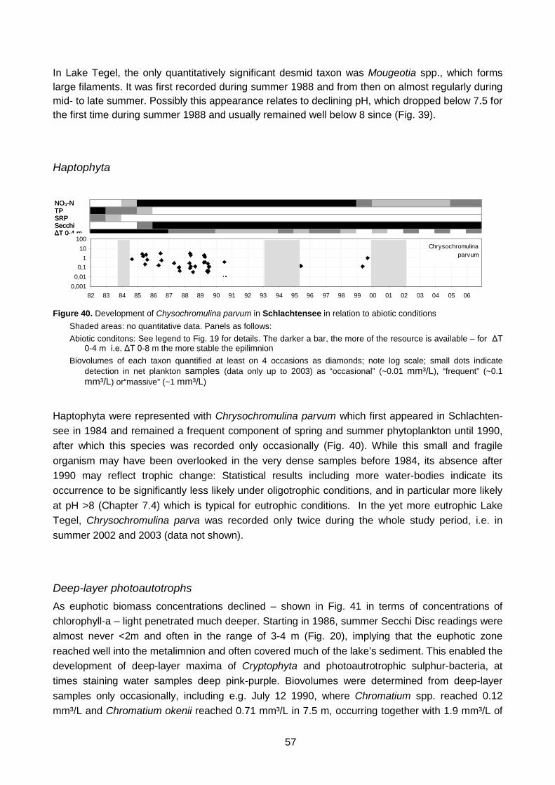
57

In Lake Tegel, the only quantitatively significant desmid taxon was Mougeotia spp., which forms large filaments. It was first recorded during summer 1988 and from then on almost regularly during mid- to late summer. Possibly this appearance relates to declining pH, which dropped below 7.5 for the first time during summer 1988 and usually remained well below 8 since (Fig. 39).

Haptophyta

Figure 40. Development of Chysochromulina parvum in Schlachtensee in relation to abiotic conditions Shaded areas: no quantitative data. Panels as follows: Abiotic conditons: See legend to Fig. 19 for details. The darker a bar, the more of the resource is available – for ΔT

0-4 m i.e. ΔT 0-8 m the more stable the epilimnion Biovolumes of each taxon quantified at least on 4 occasions as diamonds; note log scale; small dots indicate

detection in net plankton samples (data only up to 2003) as “occasional” (~0.01 mm³/L), “frequent” (~0.1 mm³/L) or“massive” (~1 mm³/L)

Haptophyta were represented with Chrysochromulina parvum which first appeared in Schlachten-see in 1984 and remained a frequent component of spring and summer phytoplankton until 1990, after which this species was recorded only occasionally (Fig. 40). While this small and fragile organism may have been overlooked in the very dense samples before 1984, its absence after 1990 may reflect trophic change: Statistical results including more water-bodies indicate its occurrence to be significantly less likely under oligotrophic conditions, and in particular more likely at pH >8 (Chapter 7.4) which is typical for eutrophic conditions. In the yet more eutrophic Lake Tegel, Chrysochromulina parva was recorded only twice during the whole study period, i.e. in summer 2002 and 2003 (data not shown).

Deep-layer photoautotrophs As euphotic biomass concentrations declined – shown in Fig. 41 in terms of concentrations of chlorophyll-a – light penetrated much deeper. Starting in 1986, summer Secchi Disc readings were almost never <2m and often in the range of 3-4 m (Fig. 20), implying that the euphotic zone reached well into the metalimnion and often covered much of the lake’s sediment. This enabled the development of deep-layer maxima of Cryptophyta and photoautrotrophic sulphur-bacteria, at times staining water samples deep pink-purple. Biovolumes were determined from deep-layer samples only occasionally, including e.g. July 12 1990, where Chromatium spp. reached 0.12 mm³/L and Chromatium okenii reached 0.71 mm³/L in 7.5 m, occurring together with 1.9 mm³/L of


Chrysochromulina parvum

0,0010,010,1

110

100

82 83 84 85 86 87 88 89 90 91 92 93 94 95 96 97 98 99 00 01 02 03 04 05 06


Chrysochromulina parvum

0,0010,010,1

110

100

82 83 84 85 86 87 88 89 90 91 92 93 94 95 96 97 98 99 00 01 02 03 04 05 06

58

Crytpmonas spp. Chlorophyll-a concentrations reflect this deep-layer photoautotrophic biomass (Fig. 41), with maxima sometimes in 6 and usually in 7.5 m depth. Studies of the deep-layer populations are available from Gervais (1997).

Figure 41. Trade-off between epilimnion and deep-layer phytoplankton in the course of Schlachtensee’s

trophic recovery, reflected by the decline of concentrations of chlorophyll-a in the epilimion (0-4 m) and their increase in the hypolimnion (6-7.5 m)

0

100

200

300

400

80 81 82 83 84 85 86 87 88 89 90 91 92 93 94 95 96 97 98 99 00 01 02 03 04 05

Chl

orop

hyll-

a [µ

g/L]

0 m 1 m 4 m5 m 6 m 7,5 m

59

4.2.2 Response of gross primary production to oligotrophication Ingrid Chorus and Gertrud Schlag

Trophic state has been defined as intensity of autotrophic production of organic matter (Elster 1961, 1962), and primary production rates of phytoplankton reflect this. Trophic change does not only affect plankton biomass levels in terms of “standing crop”, but also its process rates, i.e. production and loss rates. These may respond differently to trophic change, thus shifting the overall metabolism of a waterbody, either increasing or decreasing turnover rates. ‘For describing a lake’s trophic recovery in response to restoration, a measure of primary production therefore seemed desirable, and rates of photosynthesis were studied in early years of the restoration of Schlachtensee (1982/83) by Chorus (1989) as well as in 1986 by Wesseler (see Chorus & Wesseler 1988), i.e. in the second year after phytoplankton had shifted to substantially lower levels of biomass. Project funding for June 1987 to December 1990 provided an opportunity to continue these measurements in Schlachtensee for 2 further years and to conduct them in Lake Tegel for 1987-1990. Here, we show the results for primary production in both lakes and discuss the overall value of primary production analyses in lake restoration studies. Method The method applied was the measurement of oxygen production during 4-5 hour exposures of light and dark glass bottles submerged in distinct depths at intervals of 0.5-1 meters. Oxygen concen-trations were determined directly in the Winkler bottles used for exposure by titration following DIN 38412, part 13. This “oxygen method” gives rates for gross primary production (i.e. it includes respiration loss rates of the phytoplankton). Daily integral gross primary production was calculated by linear extrapolation from global irradiation during the hours of exposure in relation to total irradiaton for the respective day, using data supplied by the Meteorological Institute of the Free University of Berlin. For 1986, Wesseler extrapolated using light division hours as described by Talling (1957), and the linear extrapolation used during the other years may lead to underesti-mations particularly of photosynthesis maxima by up to 20% (see Talling 1957). A further source of potential underestimation of some maxima is supersaturation by 150-210% in surface-near layers during hypertrophic conditions, which occurred during hypertrophic conditions on a few occasions with particularly high insolation; this may result in losses by degassing upon opening the bottles. Depth profiles of gross primary production As shown in previous chapters, the most pronounced response to trophic change occurred in Schlachtensee between 1983 and 1986 due to the substantial decline of biomass concentrations, with water becoming much clearer. Depth profiles of oxygen production strongly reflect his: on most measuring occasions in 1986-1989, photosynthesis occurred down to depths of 4-5 m or more with rates measurable even with the rather insensitive oxygen method, while during 1982-83 rates were below the detection level already at 2-3 m depth. Fig. 42 illustrates depth profiles of photosynthesis for Schlachtensee using selected data in 1982 and 1988 (see Chorus and Wesseler 1987 for more depth profiles). In response to restoration the depth of the euphotic zone (i.e. that in which photosynthesis takes place) increased from rarely more than 2-3m in 1982-1983 to usually at least 4 m and sometimes more than 6 m in 1986.

60

Schlachtensee 1982

Schlachtensee 1988

Lake Tegel 1988

Figure 42. Selected profiles of gross primary production in g O2 l-1 h-1 (horizontal axes) over depth (in m; vertical axes) as means of exposure times (4-5 hours during noontime)

Data for 1982/1983 from Chorus (1989) and Chorus and Wesseler (1987)

25.04.

0,0 0,20

1

2

3

4

5

602.05.

0,0 0,2 0,40

1

2

3

4

5

609.05.

0,0 0,2 0,40

1

2

3

4

5

617.05.

0,0 0,2 0,40

1

2

3

4

5

625.05.88

0,0 0,2 0,4 0,60

1

2

3

4

5

630.05.

0,0 0,2 0,40

1

2

3

4

5

6

06.06.

0,0 0,20

1

2

3

4

5

613.06.

0,0 0,2 0,40

1

2

3

4

5

6

21.06.

0,0 0,20

1

2

3

4

5

6

27.06.

0,0 0,20

1

2

3

4

5

6

03.08.

0,0 0,20

1

2

3

4

5

6

16.08.88

0,0 0,2 0,40

1

2

3

4

5

6

08.09.88

0,0 0,2 0,40

1

2

3

4

5

6

20.09.

0,0 0,20

1

2

3

4

5

6

18.10.

0,0 0,20

1

2

3

4

5

6

02.11.

0,0 0,20

1

2

3

4

5

604.07.

0,0 0,20

1

2

3

4

5

6

20.07.

0,0 0,20

1

2

3

4

5

625.04.

0,0 0,20

1

2

3

4

5

602.05.

0,0 0,2 0,40

1

2

3

4

5

609.05.

0,0 0,2 0,40

1

2

3

4

5

617.05.

0,0 0,2 0,40

1

2

3

4

5

625.05.88

0,0 0,2 0,4 0,60

1

2

3

4

5

630.05.

0,0 0,2 0,40

1

2

3

4

5

6

06.06.

0,0 0,20

1

2

3

4

5

613.06.

0,0 0,2 0,40

1

2

3

4

5

6

21.06.

0,0 0,20

1

2

3

4

5

6

27.06.

0,0 0,20

1

2

3

4

5

6

03.08.

0,0 0,20

1

2

3

4

5

6

16.08.88

0,0 0,2 0,40

1

2

3

4

5

6

08.09.88

0,0 0,2 0,40

1

2

3

4

5

6

20.09.

0,0 0,20

1

2

3

4

5

6

18.10.

0,0 0,20

1

2

3

4

5

6

02.11.

0,0 0,20

1

2

3

4

5

604.07.

0,0 0,20

1

2

3

4

5

6

20.07.

0,0 0,20

1

2

3

4

5

6

24.03.82

0 0,2 0,4 0,60

1

2

3

4

5

6

26.04.82

0 0,2 0,4 0,60

1

2

3

4

5

6

10.05.82

0 0,2 0,4 0,6 0,8 1 1,2 1,40

1

2

3

4

5

6

24.05.

0 0,20

1

2

3

4

5

6

07.06.82

0 0,2 0,4 0,6 0,80

1

2

3

4

5

6

21.06.82

0 0,2 0,40

1

2

3

4

5

6

02.07.82

0 0,2 0,4 0,60

1

2

3

4

5

6

19.07.82

0 0,2 0,4 0,6 0,80

1

2

3

4

5

6

09.08.82

0 0,2 0,4 0,6 0,80

1

2

3

4

5

6

06.09.82

0 0,2 0,4 0,6 0,80

1

2

3

4

5

6

20.09.82

0 0,2 0,4 0,60

1

2

3

4

5

6

11.10.82

0 0,2 0,4 0,60

1

2

3

4

5

6

01.11.82

0 0,2 0,40

1

2

3

4

5

6

22.11.

0 0,20

1

2

3

4

5

6

24.03.82

0 0,2 0,4 0,60

1

2

3

4

5

6

26.04.82

0 0,2 0,4 0,60

1

2

3

4

5

6

10.05.82

0 0,2 0,4 0,6 0,8 1 1,2 1,40

1

2

3

4

5

6

24.05.

0 0,20

1

2

3

4

5

6

07.06.82

0 0,2 0,4 0,6 0,80

1

2

3

4

5

6

21.06.82

0 0,2 0,40

1

2

3

4

5

6

02.07.82

0 0,2 0,4 0,60

1

2

3

4

5

6

19.07.82

0 0,2 0,4 0,6 0,80

1

2

3

4

5

6

09.08.82

0 0,2 0,4 0,6 0,80

1

2

3

4

5

6

06.09.82

0 0,2 0,4 0,6 0,80

1

2

3

4

5

6

20.09.82

0 0,2 0,4 0,60

1

2

3

4

5

6

11.10.82

0 0,2 0,4 0,60

1

2

3

4

5

6

01.11.82

0 0,2 0,40

1

2

3

4

5

6

22.11.

0 0,20

1

2

3

4

5

6

13.04.88

0,0 0,2 0,4 0,60

1

2

3

4

5

610.05

0,0 0,20

1

2

3

4

5

6

24.05.

0,0 0,20

1

2

3

4

5

6

14.06.

0,0 0,20

1

2

3

4

5

6

28.06.88

0,0 0,2 0,40

1

2

3

4

5

626.07.88

0,0 0,2 0,4 0,6 0,80

1

2

3

4

5

612.07.88

0,0 0,2 0,4 0,60

1

2

3

4

5

623.08.88

0,0 0,2 0,4 0,6 0,80

1

2

3

4

5

6

27.09.

0,0 0,20

1

2

3

4

5

6

13.09.88

0,0 0,2 0,4 0,60

1

2

3

4

5

6

17.11.

0,0 0,20

1

2

3

4

5

611.10.88

0,0 0,2 0,4 0,60

1

2

3

4

5

625.10.88

0,0 0,2 0,4 0,60

1

2

3

4

5

613.04.88

0,0 0,2 0,4 0,60

1

2

3

4

5

610.05

0,0 0,20

1

2

3

4

5

6

24.05.

0,0 0,20

1

2

3

4

5

6

14.06.

0,0 0,20

1

2

3

4

5

6

28.06.88

0,0 0,2 0,40

1

2

3

4

5

626.07.88

0,0 0,2 0,4 0,6 0,80

1

2

3

4

5

612.07.88

0,0 0,2 0,4 0,60

1

2

3

4

5

623.08.88

0,0 0,2 0,4 0,6 0,80

1

2

3

4

5

6

27.09.

0,0 0,20

1

2

3

4

5

6

13.09.88

0,0 0,2 0,4 0,60

1

2

3

4

5

6

17.11.

0,0 0,20

1

2

3

4

5

611.10.88

0,0 0,2 0,4 0,60

1

2

3

4

5

625.10.88

0,0 0,2 0,4 0,60

1

2

3

4

5

613.04.88

0,0 0,2 0,4 0,60

1

2

3

4

5

610.05

0,0 0,20

1

2

3

4

5

6

24.05.

0,0 0,20

1

2

3

4

5

6

14.06.

0,0 0,20

1

2

3

4

5

6

28.06.88

0,0 0,2 0,40

1

2

3

4

5

626.07.88

0,0 0,2 0,4 0,6 0,80

1

2

3

4

5

612.07.88

0,0 0,2 0,4 0,60

1

2

3

4

5

623.08.88

0,0 0,2 0,4 0,6 0,80

1

2

3

4

5

6

27.09.

0,0 0,20

1

2

3

4

5

6

13.09.88

0,0 0,2 0,4 0,60

1

2

3

4

5

6

17.11.

0,0 0,20

1

2

3

4

5

611.10.88

0,0 0,2 0,4 0,60

1

2

3

4

5

625.10.88

0,0 0,2 0,4 0,60

1

2

3

4

5

613.04.88

0,0 0,2 0,4 0,60

1

2

3

4

5

610.05

0,0 0,20

1

2

3

4

5

6

24.05.

0,0 0,20

1

2

3

4

5

6

14.06.

0,0 0,20

1

2

3

4

5

6

28.06.88

0,0 0,2 0,40

1

2

3

4

5

626.07.88

0,0 0,2 0,4 0,6 0,80

1

2

3

4

5

612.07.88

0,0 0,2 0,4 0,60

1

2

3

4

5

623.08.88

0,0 0,2 0,4 0,6 0,80

1

2

3

4

5

6

27.09.

0,0 0,20

1

2

3

4

5

6

13.09.88

0,0 0,2 0,4 0,60

1

2

3

4

5

6

17.11.

0,0 0,20

1

2

3

4

5

611.10.88

0,0 0,2 0,4 0,60

1

2

3

4

5

625.10.88

0,0 0,2 0,4 0,60

1

2

3

4

5

6

61

However, lower phytoplankton density also resulted in substantially lower maximal production rates (amax) in surface-near layers, i.e. depth profiles changed shape (Fig. 42). A further change is that under hypertrophic conditions with poor light penetration, maximal primary production rates were observed directly under the surface, while in clearer water, until late September they occurred at depths of up to 0.5 – 2 m (Fig. 42).

The larger Lake Tegel has a deeper epilimnion, and in consequence, during hypertrophic conditions (which still characterised the lake in 1987-1990) its phytoplankton density did not quite attain the high levels of Schlachtensee (see Chapter 4.2.2); thus until autumn photosynthesis was possible down to 4-5 m (Fig. 42). This may be due to the larger phytoplankton organisms (colonial Microcystis and Aphanizomenon instead of finely dispersed Planktothrix filaments; see chapter 4.2.2) as these allow more light to penetrate at the same biomass levels. Correspondingly, maximal primary production rates in Lake Tegel’s surface-near layers were not as high as in Schlachtensee, and they were observed at 0-0.5 m, but not deeper.

A good overall descriptor of primary production depth profiles is A/amax, the mean depth of photosynthesis profiles, i.e. the integral over depth (A) divided by the maximal rate (regardless of the depth at which it occurs (amax). Fig. 43 shows that A/amax was strikingly similar in both lakes during their hypertrophic phases and increased substantially in Schlachtensee in consequence of trophic recovery. An inverse relation of the mean depth of photosynthesis profiles to trophic state was already described by Ahlgren (1970). The annual patterns reflect low global irradiation with low A/amax in early spring and late autumn, and in some years also during the spring clearwater phase, which was pronounced in some years in both lakes even under hypertrophic conditions.

Figure 43. Mean depth of photosynthesis profiles (A/amax)

data gaps in some months due to technical issues; data for 1982/1983 from Chorus (1989) and Chorus and Wesseler (1987)

01234567

87 88 89 90

A /

a m

ax [

d/m

.h] Lake Tegel

01234567

82 83

A /

amax

[d

/ m. h]

86 87 88 89

Schlachtensee

A / a

max

[m]

A / a

max

[m]

01234567

87 88 89 90

A /

a m

ax [

d/m

.h] Lake Tegel

01234567

82 83

A /

amax

[d

/ m. h]

86 87 88 89

Schlachtensee

A / a

max

[m]

A / a

max

[m]

01234567

87 88 89 90

A /

a m

ax [

d/m

.h] Lake Tegel

01234567

87 88 89 90

A /

a m

ax [

d/m

.h] Lake Tegel

01234567

82 83

A /

amax

[d

/ m. h]

86 87 88 89

Schlachtensee

01234567

82 83

A /

amax

[d

/ m. h]

86 87 88 89

Schlachtensee

A / a

max

[m]

A / a

max

[m]

62

Integrals of gross primary production The amount of primary production possible under a square meter of lake surface, i.e. integral photosynthesis (A) largely depends on two other integrals – those of the amount of biomass to produce it and of the amount of light penetrating into the water providing energy (Fig. 44).

Figure 44. Integrals of gross primary production (A; black curves) in Schlachtensee and Lake Tegel in relation to

• integrals of euphotic biovolume (BVeu; areas shaded green); • turnover rates (A / BVeu; bold red curves in areas shaded green), i.e. carbon assimilated

divided by carbon in the euphotic biovolume; • global irradiation at the day of sampling (Io; areas shaded yellow; sampling dates differ

between lakes); • light exploitation efficiency (I / Io; thin red cures in areas shaded yellow) i.e. amount of oxygen

produced divided by light energy impinging on the lake surface; note: depths of primary production and biovolume integrals vary between sampling dates; years are marked for January

The integrals of phytoplankton biovolume over the euphotic depth (BVeu) were calculated by identifying the lowest depth in which photosynthesis still occurred (from the data shown in

/ J ] / J ] / J ]

86 87 88 890

30

60

90

120

BV

eu [c

m³/m

²]

0

4

8

12

16

82 83

A /

d [g

O2

/ m². d

]

turn

ove

r ra

te [d

]

0

4

8

12

16

82 83

A /

d [g

O2

/ m². d

]

turn

ove

r ra

te [d

] Schlachtensee

AA

/ BV

eu

BVeu

I o[k

J / c

m²d

-1]

4

3

2

1

0

I o

A / I

o

A

0

5

10

15

20

82 83

A /

dA

/ Io

0

10

20

30

40

86 87 88 890

10

20

30

40

biovolumeA / d

turnover rate

A [gO2 / m² d-1]

BVeu [cm³ / m²]

A / BVeu [d-1]

Io [kJ / cm² d-1]

A / Io [gO2 / kJ / cm²]

Legend:

Lake Tegel

I o[k

J / c

m²d

-1]4

3

2

1

0

I o

BVeu

0

4

8

12

16

87 88 89 90

A /

d [g

O2

/ m².d

] tu

rnov

er ra

te [d

]

0

100

200

300

400

BV

eu [c

m³/m

²]

AA

/ BV

eu

0

5

10

15

20

87 88 89 90

A /

d

0

10

20

30

40

A /

Io

A

A / I

o

120

90

60

30

BVeu

86 87 88 890

30

60

90

120

BV

eu [c

m³/m

²]

86 87 88 890

30

60

90

120

BV

eu [c

m³/m

²]

86 87 88 890

30

60

90

120

BV

eu [c

m³/m

²]

0

4

8

12

16

82 83

A /

d [g

O2

/ m². d

]

turn

ove

r ra

te [d

]

0

4

8

12

16

82 83

A /

d [g

O2

/ m². d

]

turn

ove

r ra

te [d

]

0

4

8

12

16

82 83

A /

d [g

O2

/ m². d

]

turn

ove

r ra

te [d

]

0

4

8

12

16

82 83

A /

d [g

O2

/ m². d

]

turn

ove

r ra

te [d

] Schlachtensee

AA

/ BV

eu

BVeu

I o[k

J / c

m²d

-1]

4

3

2

1

0

I oI o

[kJ

/ cm

²d-1

]

4

3

2

1

0

I o

A / I

o

A

0

5

10

15

20

82 83

A /

dA

/ Io

0

10

20

30

40

86 87 88 890

10

20

30

40

biovolumeA / d

turnover rate

A [gO2 / m² d-1]

BVeu [cm³ / m²]

A / BVeu [d-1]

Io [kJ / cm² d-1]

A / Io [gO2 / kJ / cm²]

Legend:

Lake Tegel

I o[k

J / c

m²d

-1]4

3

2

1

0

I o

BVeu

0

4

8

12

16

87 88 89 90

A /

d [g

O2

/ m².d

] tu

rnov

er ra

te [d

]

0

100

200

300

400

BV

eu [c

m³/m

²]

AA

/ BV

eu

0

5

10

15

20

87 88 89 90

A /

d

0

10

20

30

40

A /

Io

A

A / I

o

120

90

60

30

BVeu

biovolumeA / d

turnover rate

A [gO2 / m² d-1]

BVeu [cm³ / m²]

A / BVeu [d-1]

Io [kJ / cm² d-1]

A / Io [gO2 / kJ / cm²]

Legend:

Lake Tegel

I o[k

J / c

m²d

-1]4

3

2

1

0

I o

BVeu

0

4

8

12

16

87 88 89 90

A /

d [g

O2

/ m².d

] tu

rnov

er ra

te [d

]

0

100

200

300

400

BV

eu [c

m³/m

²]

AA

/ BV

eu

0

5

10

15

20

87 88 89 90

A /

d

0

10

20

30

40

A /

Io

A

A / I

o

120

90

60

30

biovolumeA / d

turnover rate

A [gO2 / m² d-1]

BVeu [cm³ / m²]

A / BVeu [d-1]

Io [kJ / cm² d-1]

A / Io [gO2 / kJ / cm²]

Legend:

Lake Tegel

I o[k

J / c

m²d

-1]4

3

2

1

0

I o

BVeu

0

4

8

12

16

87 88 89 90

A /

d [g

O2

/ m².d

] tu

rnov

er ra

te [d

]

0

100

200

300

400

BV

eu [c

m³/m

²]

AA

/ BV

eu

0

5

10

15

20

87 88 89 90

A /

d

0

10

20

30

40

A /

Io

A

A / I

o

biovolumeA / d

turnover rate

biovolumeA / d

turnover rate

biovolumeA / d

turnover rate

A [gO2 / m² d-1]

BVeu [cm³ / m²]

A / BVeu [d-1]

Io [kJ / cm² d-1]

A / Io [gO2 / kJ / cm²]

Legend:

Lake Tegel

I o[k

J / c

m²d

-1]4

3

2

1

0

I oI o

[kJ

/ cm

²d-1

]4

3

2

1

0

I o

BVeu

0

4

8

12

16

87 88 89 90

A /

d [g

O2

/ m².d

] tu

rnov

er ra

te [d

]

0

100

200

300

400

BV

eu [c

m³/m

²]

0

4

8

12

16

87 88 89 90

A /

d [g

O2

/ m².d

] tu

rnov

er ra

te [d

]

0

100

200

300

400

BV

eu [c

m³/m

²]

AA

/ BV

eu

0

5

10

15

20

87 88 89 90

A /

d

0

10

20

30

40

A /

Io

0

5

10

15

20

87 88 89 90

A /

d

0

10

20

30

40

A /

Io

0

5

10

15

20

87 88 89 90

A /

d

0

10

20

30

40

A /

Io

0

5

10

15

20

87 88 89 90

A /

d

0

10

20

30

40

A /

Io

0

5

10

15

20

87 88 89 90

A /

d

0

10

20

30

40

A /

Io

A

A / I

o

A

A / I

o

120

90

60

30

BVeu

A

I o

A / I

o

I o

A / I

o

[g / J ]

63

Fig. 42) and integrating the biovolume from 0 m down to that depth. However, we could not determine integrals of photon flux density due to lacking light extinction data and therefore used the global irradiation impinging on the lake surfaces (Io) as an indicator of light availability. Fig. 44 shows primary production integrals (black curves) in relation to integrals of euphotic biovolume (areas shaded green) and to global irradiation (areas shaded yellow). It includes turnover rates (A/BVeu; red curves), i.e. production in terms of C assimilated per carbon content of biomass (assuming that 1 g O2 = 0.32 g C and 1 cm³ biovolume = 0.1 g C) as well as the ratio of primary production integrals to global irradiation (A/Io in g O2/J).

The most striking result is the overall similarity of the annual course of integral gross primary production (A) for all years and both lakes. In 1982/83 the euphotic zone of Schlachtensee reached only down to 2-3 meters depth whereas in later years, photosynthesis reached down to 4-6 meters. That deeper euphotic zone largely compensates the lower biomass near the surface. In other words: in the clearer water, the phytoplankton population that circulates in the epilimnion can contribute much more primary production even while being entrained into the lower part of the epilimnion, while previously substantially less light reached depths of 3-5 meters. Thus, a differently distributed phytoplankton biomass continues to produce almost as much oxygen – indicating that it assimilates almost as much carbon as during hypertrophic times, and the pronounced changes in depth distribution of primary production in response to the dramatic trophic changes in Schlachtensee between 1982/83 and 1986 caused only a rather minor reduction of integral primary production (Fig. 44).

For Lake Tegel, we did not expect much change because up to 1990 phytoplankton had not yet shown much response to restoration. Integral euphotic biovolume was lower during spring and summer of 1989, in part due to the onset of phosphorus limitation and due to a change of hydrophysical conditions allowing more stratification (see chapter 4.2.2). Also, global irradiation during summer was lower on a larger number of sampling days than in the other years, and these factors together resulted in fewer days with integral photosynthesis >10 g O2 / m² (Fig. 44).

Table 2. Annual gross primary production per m² lake surface in g O2 m-2 d-1

Note: these annual sums are estimated for March to November, but rates in winter are so low they would hardly increase these (n.d. = no data); multiply by 0.32 to obtain g carbon

1982 1986 1988 1989 1990

Schlachtensee 1255 ~1200 with estimate for Oct.-Nov.; 1026 without

1042 (1.5.88-30.4.89)

n.d. n.d.

Lake Tegel n.d. n.d. 1648 1250 1572

The lack of a substantial reduction of gross integral primary production is evident in the total annual sums (Tab. 2) estimated from the 2-4 measuring dates per month from March to November (winter rates were too low to measure with the oxygen production method, and we missed the early spring rates in some years due to an instable ice cover): For Schlachtensee after 1982, data are not available for one complete calendar year, but the time span from May 1988 to April 1989 amounts to a full year. Also, from the data for other years we can

64

roughly estimate the missing data for Oct.-Nov. 1986 to amount to 100-150 g O2 m-2 d-1, and if we add this, the annual sum for 1986 would amount to roughly 1200 g O2 m-2 d-1. Thus, annual sums decreased somewhat in 1986 and 1988/89 as compared to 1982, but only by about 25%. In Lake Tegel, annual integrals were slightly higher than in Schlachtensee (Tab. 2), possibly reflecting the slightly deeper euphotic zone even during hypertrophic times.

With 1 g O2 produced corresponding to 0.32 g C, annual gross production in Schlachtensee in 1982/82 as well as in Lake Tegel from 1987-1990 corresponded to 400-500 g C assimilated per m² and year. This is in the range classified as “polluted eutrophic” by Rodhe (1958) and in the upper range of 47 lakes described by LeCren and Lowe-McConnell (1980). Schlachtensee in 1988 with ~330 g C /m².a would still classies as eutrophic in the scheme proposed by Rodhe and barely eutrophic in the scheme given by Wetzel 1988 (the latter gives “eutrophic” is given as > 1000 mg C/m² and day, corresponding to 365 g/m² and year). However, these schemes give net primary production, while our data are for gross primary production, with uncertain loss rates through respiration.

Seasonal patterns of primary production in relation to light and phytoplankton biomass

Seasonal patterns of gross primary production integrals show maxima of 8-12 g O2 m-2d-1 in spring and summer, with minima occurring during the spring clearwater phase and in autumn (Fig. 44). Summer levels often followed global irradiation impinging on the lake surface (Io), if biovolume integrals were high. This is particularly conspicuous in Schlachtensee during summer 1982 and spring 1983, when phytoplankton had a rather stable species composition dominated by filamentous Osciallatoriales (see chapter 4.2.2), but also in Lake Tegel during the summers of 1987, 1988 and 1990. The extremely high biovolume integral maximum in Lake Tegel in 1990 traces back to a substantial Microcystis bloom consisting of large colonies co-occurring with high amounts of the large motile dinoflagellate Ceratium spp.. Large flagellates and large colonies create high biovolumes which cause less turbidity than would be caused the same biovolume of small-celled plankton. This enabled photosynthesis down to 4-5 m depth and thus a high integral at a low turnover rate (i.e. A/BVeu). In contrast, during the spring clearwater phase (which was more regularly and conspicuously pronounced in Lake Tegel than in Schlachtensee), phytoplankton biomass was too low to translate global irradiation into much primary production.

Primary production integrals declined in autumn, reflecting the decline of biomass and global irradiation. However in relation to global irradiation, light exploitation for photosynthesis was conspicuously high in autumn in both lakes (no data are available for Schlachtensee for autumn of 1986, 1987 and 1989; Fig. 44). This is partially due to declining, but yet relatively high levels of biovolume using the available light very effectively for photosynthesis. However, at the rather low levels of both A and Io, the relatively greater errors may also cause very high quotients of both parameters.

Chorus (1989) discussed that the data for the early years show no correlation between light exploitation efficiency (A/Io) and euphotic biomass integrals (BVeu) in Schlachtensee, contrary to observations from some other lakes, and interpreted this as being due to the very high

65

levels of euphotic biomass at most sampling and measuring occasions. This implies that photosynthesis integrals were rarely limited by biomass, but rather by light availability. This should change in response to restoration: Light exploitation efficiency should be lower, i.e. limited by BVeu, more often once euphotic biomass levels have decreased. Indeed the data for Schlachtensee 1986-1989 show summer quotients for A/Io to be lower more often than before (Fig. 45).

Analyses for the association between the light exploitation efficiency A/Io and euphotic bio-volume integrals BVeu in Schlachtensee for the data set from 1982 to 1989 show that BVeu can explain 30% of the variability of light exploitation in most cases, i.e. excluding the 3 extreme maxima of A/Io>19 g O2/kJ due to very low Io in autumn 1982, 1989 and spring 1983 (Fig. 44). In contrast, in Lake Tegel from 1987 to 1990, levels for A/Io were higher, similar to those in Schlachtensee in 1982/83 before the response to restoration. Also, just like Schlachtensee when taking only the data before restoration response, regression analyses shows more scatter and can explain only 17% of the variability of A/Io in relation to BVeu (even when excluding the 4 extreme autumn maxima; Fig. 45).

Figure 45. Light exploitation efficiency (A/Io) in relation to euphotic biovolume (BVeu)

Schlachtensee: A/Io = 0.79 ln BVeu + 1.8; R²=0.30, excluding 3 extreme maxima >19 g O2/kJ; Lake Tegel: A/Io = 1.43 ln BVeu + 0.85; R²=0.17, excluding 4 extreme maxima >19 g O2/kJ

Turnover rates – i.e. photosynthesis per unit biomass – were inverse to the euphotic biovolume integrals (Fig 44), as has been described in many studies. It is also well established that small-celled species of phytoplankton (as tend to dominate during spring clearwater phases and in less eutrophic waterbodies) usually have higher turnover rates than large ones (Wetzel 1983). The seasonal patterns observed in both lakes (Fig. 44) correspond to this expectation. So does the restoration response of turnover rates in Schlachtensee: they were very low (<1 d-1) in 1982 during a massive and persisting bloom of Planktothrix agardhii, with the exception of one sampling occasion in August 1982 the day after a rain storm hat perturbed this bloom, leading to low biovolume, but with phytoplankton showing high rates of photosynthesis. In contrast, summer turnover rates available for 1986, 1987 and 1988 were largely > 1 d-1. In the still eutrophic Lake Tegel, they were low in all four years (1987-1990), declining steadily as summer phytoplankton populations (dominated by large

Schlachtensee

0

4

8

12

16

0 50 100 150

BV eu [cm³ / m²]

A /

Io [

g O

2 / k

J]

Lake Tegel

0

4

8

12

16

0 50 100 150 200 250 300 350

BV eu [cm³ / m²]

A /

Io

[g O

2 / k

J]

Schlachtensee

0

4

8

12

16

0 50 100 150

BV eu [cm³ / m²]

A /

Io [

g O

2 / k

J]

Lake Tegel

0

4

8

12

16

0 50 100 150 200 250 300 350

BV eu [cm³ / m²]

A /

Io

[g O

2 / k

J]

66

colony-forming cyanobacteria) increased, with minor peaks in late summer or early autumn of some years.

Figure 46. Photosynthetic capacity (amax) in relation to Chl.a at the depth of amax: Schlachtensee: amax = 0.0044 Chl.a + 0,13; R²=0.49 excluding 2 extremely high values of 0.9 and 1.54 in spring 1982 (open diamonds) R²=0.73

Lake Tegel: amax = 0.0059 Chl.a + 0.16; R²=0.59

A specific case of turnover is the photosynthetic capacity, i.e. the ratio of the maximal photo-synthesis determined in each depth profile, i.e. amax, to the phytoplankton biomass at that depth, quantified in terms of concentrations of chlorophyll-a. Where maximal rates of photosynthesis do not occur directly at the lake surface, but in 0.5 m depth or more, we may assume them to be light saturated. Fig. 46 shows that amax closely followed the concentrations of chlorophyll-a measured at the depth of amax in both lakes and at almost all occasions. For Lake Tegel, regression analysis shows a quite linear relationship; chlorophyll-a measured at the depth of amax can explain 59% of the variability of amax. For Schlachtensee, this correlation is not as tight (R²= 0.49) because of two extremely high values of 0.9 and 1.54 in spring 1982 (without these, R² is 0.73). Furthermore, in 1982/83 during the pronounced dominance of Oscillatoriales, amax was somewhat lower in relation to concentrations of chlorophyll-a. A further determinant of amax is temperature: this determines

Lake Tegel

0,0

0,4

0,8

1,2

1,6

0 50 100 150 200Chl.a at depth of amax [µg/L]

amax

[m

g / L

. h]

Schlachtensee

0,0

0,4

0,8

1,2

1,6

0 50 100Chl.a at depth of amax [µg/L]

amax

[m

g / L

. h]

Lake Tegel

0,0

0,4

0,8

1,2

1,6

0 50 100 150 200Chl.a at depth of amax [µg/L]

amax

[m

g / L

. h]

Schlachtensee

0,0

0,4

0,8

1,2

1,6

0 50 100Chl.a at depth of amax [µg/L]

amax

[m

g / L

. h]a m

ax [m

g O

2 L-1 h

-1]

0,0

0,5

1,0

1,5

2,0

82 83

a m

ax [m

g O

2 / L

. h]

86 87 88 890

0,5

1

1,5

2

Chl.-a

a max

200

150

100

50

0

Chl

.-aat

am

ax[µ

g/L]

Schlachtensee

87 88 89 90

200

150

100

50

0

Chl

.-aat

am

ax[µ

g/L]

Lake Tegel2,0

1,5

1,0

0,5

0

am

ax[m

g O

2/ L

. h]

283

0,0

0,5

1,0

1,5

2,0

82 83

a m

ax [m

g O

2 / L

. h]

86 87 88 890

0,5

1

1,5

2

0,0

0,5

1,0

1,5

2,0

82 83

a m

ax [m

g O

2 / L

. h]

86 87 88 890

0,5

1

1,5

2

Chl.-a

a max

200

150

100

50

0

Chl

.-aat

am

ax[µ

g/L]

Schlachtensee

87 88 89 90

200

150

100

50

0

Chl

.-aat

am

ax[µ

g/L]

Lake Tegel2,0

1,5

1,0

0,5

0

am

ax[m

g O

2/ L

. h]

283Chl.-a

a max

200

150

100

50

0

Chl

.-aat

am

ax[µ

g/L]

Schlachtensee

87 88 89 90

200

150

100

50

0

Chl

.-aat

am

ax[µ

g/L]

Lake Tegel2,0

1,5

1,0

0,5

0

am

ax[m

g O

2/ L

. h]

Chl.-a

a max

Chl.-a

a max

200

150

100

50

0

Chl

.-aat

am

ax[µ

g/L]

Schlachtensee

87 88 89 90

200

150

100

50

0

Chl

.-aat

am

ax[µ

g/L]

200

150

100

50

0

Chl

.-aat

am

ax[µ

g/L]

Lake Tegel2,0

1,5

1,0

0,5

0

am

ax[m

g O

2/ L

. h]

283

67

rates of photosynthesis only in the depth at light saturation, while below, light limits rates of photosynthesis, and Chorus (1989) shows an increase of photosynthetic capacity with temperature for Schlachtensee in 1982/83. However, temperature dependence has rather little relevance for restoration response, as it affects only part of the integral gross photosynthesis under a m² of lake surface.

Predicting gross primary production For Schlachtensee, the relationship between Io and A is statistically significant, with Io explaining 36% of the variability of A (R²=0.36), while for Lake Tegel (R²=0.08), there is more scatter due to the high fraction of data collected during the clearwater phase. In contrast, for Lake Tegel, the euphotic biovolume integrals explain 42% of the variability of A, while for Schlachtensee this R² amounts to only 0.12 (Fig. 47).

Figure 47. Regression analyses of integral gross primary production in relation to

Io: Schlachtensee: A= 0.96 Io + 2,5, R²=0.36; Tegel: A= 1.2 Io + 4.0, R²=0.08

ln BVeu: Schlachtensee: A= 2.4 ln BVeu + 1.9, R²=0.12; Tegel: A= 2.1 ln BVeu – 1.1, R²=0.52

Multivariate regression analysis showed that Io and BVeu together explain 42% - 55% of the variation of integral gross primary production in Schlachtensee and Lake Tegel, respectively:

Schlachtensee: A = 2.2 Io + 0.87 ln (BVeu) -0.34; R²=0.42

Lake Tegel: A = 1.6 Io + 2.3 ln (BVeu) -3.6; R²=0.55

Furthermore, although these regression equations result in somewhat different factors for the data of each lake, joint analysis of the data for both lakes give an R² of 0.45 and shows that the “factor lake” does not improve the explanatory power of the model describing the association between gross integral primary production and the two variables determining it,

Integrals of gross primary production (A) against global irradiation (Io) Schlachtensee Lake Tegel

0

4

8

12

16

0,0 1,0 2,0 3,0 4,0Global Irradiation (Io) [kJ / cm² d -1]

Prim

ary

Pro

duct

ion

(A)

[g /

m² d

-1]

0

4

8

12

16

0 100 200 300Euphotic Biovolume (Bveu) [cm³ / m²]

Prim

ary

Pro

duct

ion

(A)

[g /

m² d

-1]

0

4

8

12

16

0,0 0,5 1,0 1,5 2,0 2,5 3,0 3,5

Global Irradiation (Io) [kJ / cm² d -1]

Prim

ary

Prod

uctio

n (A

) [g

/ m

² d -1

]

0

4

8

12

16

0 20 40 60 80 100Euphotic Biovolume (BVeu) [cm³ / m²]

Prim

ary

Prod

uctio

n (A

) [g

/ m

² d -1

]

Integrals of gross primary production (A) against integral euphotic biovolume (ln BVeu)

68

i.e. global irradiation and integral euphotic biovolume. This implies that the relationship between both factors and A exists irrespectively of the lake:

Data of both lakes : A = 1.7 Io + 1.7 ln (BVeu) -2.0; R²=0.45

A tighter association with light availability is likely when using better information for photon flux density in the euphotic zone, i.e. with data on light extinction coefficients and calculations of integrals or means of photon flux density (rather than using global irradiation indicator).

For lake restoration studies, this result implies that from phytoplankton biovolume and light availability, it is possible to predict annual integral gross primary production of the phytoplankton, though with some uncertainty. Fig. 44 shows that during summer, particularly under conditions with rather stable phytoplankton populations as in Lake Tegel in 1987, 1988 and 1990, A follows both Io and BVeu quite closely, suggesting that a more detailed model that depicts seasonal patterns would further reduce the uncertainty of such predictions.

Value of primary production data for understanding trophic recovery The most interesting result of the primary production measurements for the overall metabolism of the lakes – i.e. production versus degradation of organic matter – is the rather minor restoration response of depth-integrated gross photosynthesis observed in Schlachtensee up to 1989: the pronounced reduction of biomass densities and rates of photosynthesis per liter was largely compensated by an increased depth of the euphotic zone. This means that during the late 1980’s photosysnthesis produced almost as much organic carbon as in 1982/1983, and this undergoes mineralisation, consuming oxygen through the respiration of zooplankton and microbial communities. This implies a delay in the recovery of the lake’s oxygen budget (see below, Fig. 48).

While no primary production data are available for the 1990’s and the 2000’s, in face of the further decline of phytoplankton biomass particularly after 2000 (Fig. 20) a more pronounced reduction of integral gross primary production (i.e. per m² lake surface) is likely for two reasons: (i) there is little room for further compensation through an increasingly deep euphotic zone: with ~5 m by the end of the 1980s it had already reached the sediment in much of the lake; (ii) while the restoration response decreases turbidity from planktonic particles, light adsorption by the water itself remains constant, setting a further limit to the compensation by increased vertical extension of photosynthesis.

No data are available for rates of photosynthesis after 1989, but photosynthesis integrals could be modelled from integrals of biovolume or chlorophyll-a per m² lake surface and from integrals of photon flux which can be inferred from Secchi disk data, drawing on data for photon flux intensity which are available for some years in the 2000’s (not shown here). This would be a worthwhile future work package for a better understanding of the restoration response of the lake’s metabolism, and for its non-linear response mechanisms.

69

4.2.3 Further ecosystem responses Ingrid Chorus The pronounced reduction of phytoplankton biomass concentratins in Schlachtensee induced a cascade of consequences for other ecosystem components, briefly outlined as follows:

Zooplankton Zooplankton populations are expected to respond to lake restoration because of (i) the pronounced changes in their food, i.e. phytoplankton biomass and species composition, (ii) of the deeper extension of their habitat as the anoxic zone becomes smaller, and (iii) increasing opportunities for grazing protection as macrophyte stands recover. For Schlachtensee, zooplankton data are available for the lake’s hypertrophic phase (1982-1983), for parts of the years 1985 (i.e. the year of the steepest decrease of phytoplankton biomass) and 1986, and continuously for two years under mesotrophic conditiones, i.e. from May 1987 to June 1989 (Ewald 1991).

For strongly eutrophic lakes, the PEG model (Sommer et al. 1986) describes steep vernal maxima, minima in early summer and some minor maxima in late summer, and in 1982/83 Schlachtensee’s zooplankton matched this model: Spring maxima were extremely steep, with around 1600 individuals per liter, strongly dominated by small cladocerans (mostly Bosmina longirostris) whose high abundance indicates a food chain based on detritus, with zooplankton exerting less grazing pressure on phytoplankton. For oligotrophic stratifying lakes, the PEG model describes a slower increase throughout spring and early summer to one summer maximum (Sommer et al. 1986). For the Schlachtensee data 1986-1989, Ewald (1991) discusses an “in between” state, with slight spring maxima (400-600 individuals per liter) and higher summer populations, due to an increase of the populations of Daphnia spp. and Diaphanozoma mongolianum (their maxima were 2-4 fold higher than during 1982/83). Also, zooplankton shifted to a higher share of cladocerans filtering coarser particles as compared to the fine-filtering Bosmina in 1982/83, and to larger individuals. Zooplankton growth was supported by a reduction of the planktivorous fish stock through a fish kill of adult Abramis brama in 1982/83 and in the following years by fishery measures to reduce the stock of cyprinid fish.

Thus, key features of the zooplankton response to restoration in Schlachtensee were the smoother seasonal pattern (particularly with less pronounced spring maxima) and the reduction of fine-filtering cladocerans.

For Lake Tegel, data on zooplankton biomass and species composition were studied by Köhler (Köhler & Chorus 2010) for 1993-2003, i.e. including the phase of the lake’s most pronounced oligotrophication response in 1995-1996. However, oligotrophication had not yet reached the low levels of Schlachtensee, and seasonal patterns still show the pronounced spring and late summer maxima described as typical for eutrophic lakes by Sommer et al (1986), with clear-water phases (Secchi depths of up to 4 m) in May largely due to grazing pressure. Copepod maxima in March and April were followed by larger numbers of cladocera, mainly Daphnia galeata but also smaller species like Bosmina longirostris and

70

Eubosmina coregoni thersites in later spring. In autumn, the zooplankton was dominated by calanoid copepods (Eudiaptomus gracilis) and rotifers (Polyarthra spp., Synchaeta spp.).

Towards the end of the 1990s, both the absolute zooplankton amounts and species composition stabilised, with maxima less pronounced. Local fishermen attribute pronounced reductioins of their catches to the reduced phytoplankton biomass since 1994: among the cyprinid fish the 0+ age group declided and pike perch migrated from Lake Tegel to the more turbid waters of the adjacent River Havel. Grazing pressure on zooplankton partially shifted from fish to the carnivorous cladoceran predator Leptodora sp. and this favoured larger species e.g. of Daphnia (with the mean body mass of D. galeata increasing 2-fold) better able to escape predation by Leptodora. While the increase of Microcystis spp. in 1997–2002 can be explained by re-eutrophication, the higher grazing pressure by large Daphnia on edible phytoplankton will have contributed to dominance of these poorly edible colonial cyanobactiera (Köhler & Chorus 2010).

Overall, in Lake Tegel as in Schlachtensee, phytoplankton was largely controlled “bottom-up”, i.e. by resource availability, whereas “top-down” control by grazing was relevant chiefly in spring. In both lakes, population changes in zooplankton were not as pronounced as those observed for the phytoplankton, i.e. phytoplankton changes did not directly translate 1:1 to zooplankton changes, and this likely due to the influence of feeding pressure from planktovorous fish.

Schlachtensee’s oxygen budget In addition to direct oxygen exchange with the atmosphere, production through photosynthesis and consumption through the mineralisation of organic matter strongly shape a lake’s oxygen budget. Provided trophic recovery reduces primary production – not only in terms of rates per m³ of water, but also as integrals per m² lake surface – it should become manifest in a lake’s oxygen budget.

During their hypertrophic phase, both lakes had shown pronounced hypolimnetic anoxia during summer, with a strong smell of hydrogren sulphide in deepwater samples from Schlachtensee. While the oxygen budget of Lake Tegel was influenced by artificial aeration, in Schlachtensee, changes over time directly reflect oligotrohication: In 1980-1985 conditions with <1 mg/L O2 climbed up to 4 m depth; from 1987-1990 <1 mg/L O2 were observed only up to 5 m depth, and from 1991-1995 only up to 6 m depth. 1986 was an exception with more than 1 mg/L O2 in 6 m throughout the summer (albeit at only monthly sampling). In the years since 1995, oxygen depletion below 1 mg/L was usually observed only in 7 m depth, with depletion in 6 m occurring sporadically and briefly. Likewise time spans with <1 mg/L became shorter: in the first half of the 1980s they ranged from mid-May until autumn overturn, while since 2000 in 7.5 m depth levels <1 mg/L were never observed before July.

To depict responses of the oxygen budget to restoration, similarly to the anoxic factor used by Nürnberg (1995) we calculate an oxygen deficiency index from the fraction of the lake’s water volume containing <1 mg/L O2 multiplied by the fraction of the 365 days of the year during which each layer is in this condidion (Fig. 48). The accuracy of this index is influenced by the number of measuring dates available (which varied between monthly to weekly); therefore in Fig. 48 we give the minimum index calculated from the minimum time span that

71

the respecttive lake volume contained <1 mg/L O2 (i.e. counting only the number of days with data showing <1 mg/L), the corresponding maximimum time span (i.e. assuming O2 had dropped to <1 mg/L already the day after the last sampling occasion with concentrations >1mg/L and had stayed below 1 mg/L up to the first sampling date with >1 mg/L), as well as the mean between these two extremes.

The oxygen deficiency index shows a pronounced decline (Fig. 48), first in the second half of the 1980s (although not as strongly as the concentration of Chlorophyll-a) with levels still between 0.02 and 0.03 in the first half of the 1990s and below 0.02 only since 2001. Some time lag is to be expected, as the oxygen-consuming mineralisation of organic material on the sediment surface and in its upper layers will continue for some time after the amounts sedimenting to the sediment have decreased. A pronounced change from black sapropelic mud smelling strongly of H2O in the 1980’s to a grey sandy texture by the late 1990s is evident, although no visual records are available to allocate a time line to these observations.

Figure 48. Oxygen deficiency index for Schlachtensee (black curves), i.e. the fraction of the lake’s volume and days of the year with oxygen concentrations <1 mg/L on the background of the concentrations of Chlorophyll-a at 1 m depth.

Note: the three curves show temporal integration between sampling dates for the shortest (min), the longest (max) and the mean time interval conceivable at which a water layer contained <1 mg/L O2.

The quite pronounced decrease of the oxygen deficiency index in the late 1980s is surprising in face of the rather minor decrease of depth-integrated primary production by only by about 25% (see Fig. 43). The latter implies that a large amount of organic substance was still being produced per m² lake surface, which would keep the oxygen demand for mineralisation rather high. A possible explanation is a shift of biodegradation from the sediment surface to the water column. A number of mechanisms may play a role in this, including that

1. overall lower concentrations of biomass consume less oxygen through respiration and biodegradation;

2. the switch of phytoplankton species composition to taxa which are more amenable to grazing (Chapter 4.2.2) and the increase of zooplankton (see above) causes more of the organic carbon from primary production to be eaten by zooplankton. Part of this will be mineralised by zooplankton respiration, and part be excreted as faecal pellets. While it is uncertain whether these are mineralised more rapidly than dying

0

25

50

75

100

Chl

orop

hyll-

a at

1 m

[µg

/L]

0,00

0,02

0,04

0,06

0,08

0,10

1980

1982

1984

1986

1988

1990

1992

1994

1996

1998

2000

2002

2004

2006% o

f day

s an

d la

ke v

olum

e at

<1

mg/

L

minmeanmax

0

25

50

75

100

Chl

orop

hyll-

a at

1 m

[µg

/L]

0,00

0,02

0,04

0,06

0,08

0,10

1980

1982

1984

1986

1988

1990

1992

1994

1996

1998

2000

2002

2004

2006% o

f day

s an

d la

ke v

olum

e at

<1

mg/

L

minmeanmax

0.10

0,08

0.06

0.04

0.02

0.00

0

25

50

75

100

Chl

orop

hyll-

a at

1 m

[µg

/L]

0,00

0,02

0,04

0,06

0,08

0,10

1980

1982

1984

1986

1988

1990

1992

1994

1996

1998

2000

2002

2004

2006% o

f day

s an

d la

ke v

olum

e at

<1

mg/

L

minmeanmax

0

25

50

75

100

Chl

orop

hyll-

a at

1 m

[µg

/L]

0,00

0,02

0,04

0,06

0,08

0,10

1980

1982

1984

1986

1988

1990

1992

1994

1996

1998

2000

2002

2004

2006% o

f day

s an

d la

ke v

olum

e at

<1

mg/

L

minmeanmax

0.10

0,08

0.06

0.04

0.02

0.00

72

cyanobacteria or diatoms, the process as such occurs to a larger extend during summer in warmer water with higher mineralisation rates.

A hypothesis warranting further testing is that the trophic recovery of the oxygen budget is only partially due to lower productivity, but also due to more effective mineralisation of organic matter in particles already on their way to the lake sediment, i.e. the shift in the phytoplankton community enhances mineralisation and thus drives the recovery of the oxygen budget more strongly than the overall reduction in primary production.

This change in lake metabolism leads to a further positive feed-back mechanism, as oxygenated sediments have a substantially different structure and provide a better habitat for colonisation by aquatic macrophytes and larger animals. Aquatic macrophyte beds, in turn, compete against phytoplankton for phosphorus, thus further reducing phosphorus availability for phytoplankton growth.

Macrophytes During the hypertrophic phase, submerged macrophytes were absent in both lakes and their reed belts had strongly declined. Indeed their sapropelic sediments were unsuitable for macrophyte growth even after the light climate had improved, and 5-6 years after Schlachtensee had abruptly become clearer, Machatzi and Steif (1991) still found almost no macrophytes. To protect reed belts and littoral areas from boats and waves, barriers were introduced in the 1990s, and at Schlachtensee fences were also introduced between the walking path and much of the lake shore to protect the macrophytes from the immense pressure by people and pets. Macrophytes were mapped in 2005 in Schlachtensee and in 2007 in Lake Tegel. The results at this time show almost complete coverage of the sediment down to 2.7 m depth (i.e. 20% of the lake area) in Schlachtensee, with species including Najas marina subsp. intermedia (holly-leaved pondweed), tall Myriophyllum spicatum (Eurasian water-milfoil), low-growing Chara contraria (opposite stonewort), as well as small, low growing forms of Potamogeton pectinatus (sago pondweed) and P. berchtoldii (slender-leaved pondweed) (Hilt et al. 2010). In Lake Tegel, the depth of coverage varied between 1.0 and 3.7 m, with large P. pectinatus and M. spicatum dominating and N. marina subsp. intermedia and C. demersum also abundant.

As discussed by Hilt et al. (2010), macrophytes stabilise clear conditions not only in shallow lakes, but also in stratified ones, directly by binding nutrients and indirectly through their effects on the food chain: they provide shelter for zooplankton as well as a structural habitat for piscivorous fish such as pike, which in turn reduce planktivorous fish, thus increasing population growth for zooplankton which in turn graze on phytoplankton. While the recolonisation of both lakes with macrophytes marks trophic recovery, Hilt et al. also point out that a return to the Characean communities present in the 19th century is not likely due to a lack of seed banks throughout the Berlin area.

Thus, the return of macrophyte coverage marks a late stage of trophic recovery, and a return to the species composition natural to these lakes will require oligotrophication also of their tributaries. Like fish, macrophytes have a pronounced link to the catchment and will hardly recover back to the original state in a lake physically isolated from its tributaries by a treatment plant.

73

5. Management Models Inke Schauser

The management models developed for Lake Tegel and Schlachtensee are empirical and lake specific. Common lake models are either mechanistic-dynamical and calibrated for a specific lake, e.g. Janse & Van Liere (1995), Reynolds et al. (2001), or statistical-empirical and lake unspecific, e.g. Vollenweider (1976), Vollenweider and Kerekes (1982), Jensen et al. (2006). Lake specific, empirical models combine the advantage of both approaches. They need less parameters than mechanistic models, since they do not describe the processes in detail, and they can model seasonal changes in a stratified lake with a multi-box model. The model uncertainty is less than that of statistical-empirical models since they are calibrated for the lake in question. Empirical-lake specific models can help to understand the causalities of the water and phosphorus balances better than statistical-empirical models can. Thus, it is possible to run scenarios to estimate the effects of future lake management measures and to assess the effects of former measures by data analysis. However, lake specific, empirical models have limits. They are not transferable to other lakes such as mechanistic or statistical models. Like all lake specific models their adaptation depends on good data sets in adequate temporal scale. The longer the time record for a lake, the more accurate the evaluation of unknown parameters, natural variability and the effects of former measures of the lake management. Additionally, because these management models are empirical models, the model results are not always explicable in terms of biogeochemical relationships. The significance of a variable for – e.g. the lake P concentration – and for the individual fluxes can change from one model calibration to the other. The applicability of these management models to conditions beyond those within the calibration and validation ranges is therefore limited; i.e. results of calculations beyond these ranges have a high uncertainty.

We developed and used management models for Lake Tegel and Schlachtensee to establish complete water and phosphorus balances over the past 20-25 years. The phosphorus models are 3-box models for an upper and lower water compartment as well as a sediment compartment. Processes integrated in the model are: sedimentation of P from the upper into the lower water compartment and into the sediment, mixing between the water compart-ments, and P release from the sediment into the lower water compartment.

Unknown variables were described as functions of known variables and unknown parameters. These parameter values were determined in an iterative process of calibration, optimisation and sensitivity analysis and checked for plausibility. Unknown variables of the water balance of Lake Tegel were the inflow from River Havel and the proportion of bank infiltration, for which as a first approximation we used a literature value of 80 % (Fritz et al. 2002). For Schlachtensee the unknown variables were the inflow from the storm water overflows and the surface water inflow from the direct watershed. The surface water inflow might be an important carrier of the unexplained (though in absolute terms small) P load. The unknowns of the phosphorus balance were, after the external load could be quantified by a validated water balance, mixing of the water column, as well as sedimentation and release of P from the sediment. These processes are very difficult to measure in-situ.

74

5.1 Models for the water budgets of both lakes A key issue and ongoing problem for local management of Lake Tegel had been the distinction between the inflows from the River Havel and from the Phosphorus Elimination Plant (PEP). Two different models for the inflow from the River Havel to Lake Tegel were developed and both showed good agreement and confirmed earlier estimates. Their result is that the River Havel inflow constitutes about 40 % of the total water inflow into Lake Tegel, and that water residence time is ~ 75 d. The numerical model uses the chloride balance to estimate the water balance, assuming chloride to be a perfect tracer. The calculated chloride concentration of Lake Tegel shows a very good fit with the measured values for calibration (1991-2002, r = 0.86), validation (1986-1990, r = 0.81) and for the complete data set (1986-2002, r = 0.88). The considerable inter-annual and inter-seasonal variation of the River Havel inflow to Lake Tegel can be satisfactorily predicted from River Havel discharge, PEP discharge, and water extraction (bank infiltration and recharge) by the Berlin Water Utility (Schauser & Chorus 2009).

For Schlachtensee, the water balance model also shows very good results during calibration (1995-2002, r = 0.94), validation (1987-1994, r = 0.92) and for the complete data set (1987-2002, r = 0.93). With this, the water balance can be calculated from PEP inflow, precipitation and storm water discharges as well as hypolimnion withdrawal and other outflows. Storm water discharges are of less importance for the water balance of Schlachtensee. Hydrogeologists of the Berlin Water Utility, the Free University of Berlin and the Federal Environment Agency assume only an intermittent groundwater inflow, i.e. only during winter, and then mostly as surface or subsurface flow. The water retention time was calculated to be around 220 days (Schauser & Chorus 2009).

5.2 Models for the P budgets of both lakes The P balance for both lakes was modelled on the basis of the water balance. A central aspect was the differentiation between external and internal loads and to clarify whether redox conditions (i.e. desorption) or temperature (i.e. mineralisation) are key drivers for P release from the sediments.

The P balance of Lake Tegel could be modelled very well during calibration (1990-2002, r = 0.87), validation (1985-1989, r = 0.85; 2003-2006, r = 0.32) and overall (1985-2006, r = 0.89). The fit for the P concentration when separately modelling the upper and lower water column was even better. The lake P budget of Lake Tegel is characterised by high inter-annual and seasonal differences (Fig. 12), which indicate that the lake reacts quickly to changes in the external and internal load. The mixing coefficient is rather high (kmix = 212), indicating a low stratification stability. The phosphorus model of Lake Tegel proved P sedimentation to depend mainly on the River Havel load, which overall is the most important component in the P balance of Lake Tegel, followed by the PEP discharge and the water works extractions. Internal P release was satisfactorily modelled as a function of the temperature above the sediment, stratification stability, and iron content of the sediment, with a slightly better fit being achieved if the nitrate concentration at the lake bottom is included. This iron content is a function of the iron discharge of the PEP Tegel. These results support the conclusions drawn from the time series analysis that the P release is mainly controlled by mineralisation (see chapter 4.1.3), especially in years with low iron content in the sediments. The annual

75

net sedimentation of P was calculated as difference between sedimentation and release. On an annual basis, the sediment has acted as a P sink in most years (1989, 1992-1999, 2003-2006). In years in which the sediment was a P source, the modelled internal P load is 2-4 folds larger than the annual load from the PEP, but only 0.25-1 fold of the annual River Havel load, indicating the sediments to be a relevant short-term source of P (Fig. 49). It is likely that sediment P “recharge” by the high external load is a rather short-term process, i.e. that the P released from the sediment largely is P that only recently reached the lake’s sediments from the load carried into the lake by the River Havel. In consequence, external load reduction is likely to be rapidly followed by a reduction of the internal load. 80% of the external load during recent years has originated from the River Havel, 16.5 % from the PEP Tegel, and 3.5 % from precipitation (Schauser & Chorus 2009).

Figure 49. P sources and net sedimentation in Lake Tegel (1986-2006) (Schauser & Chorus 2009)

For Lake Schlachtensee, the long-term development of the P concentration is dominated by the reduced external load from the PEP Beelitzhof. The epilimnion exerts a dominant effect on the P dynamics. Stratification stability is rather high, indicated by a low mixing coefficient (kmix = 10). Sedimentation is a function of precipitation, PEP discharge and hypolimnetic oxygen concentration, reflecting the importance of iron-phosphorus precipitation at the onset of circulation. P release can be calculated best as function of temperature above the sediment and stratification stability. In the hypolimnion, a regular accumulation of P occurs, which can be very well depicted by the model. However, the P release from the sediment has only a small influence on the overall P budget of the lake, because of the small hypolimnion volume and the stable stratification. The accumulated P settles down during winter. However, the phosphorus model produced comparatively poor results for calibration (1990-2002, r = 0.58) and validation (1985-1989, r = 0.66; 2003-2006, r = 0.24). The overall fit was better (1985-2006, r = 0.75). The same is true for the fit for the upper and lower water column. The years from 1988 to 1997 are particularly problematic, as their P concentration is characterized by late autumn and winter peaks mainly in the upper water column, which do not occur in the chloride concentration. They indicate an unknown external P source. One possible source could be dog excrements and/or leaves, particularly during October- January. Being a glacial trough, the lake has rather steep shores with pronounced erosion traces from heavy use by people and their pets. An estimation of plausibility showed that

-10

-5

0

5

10

15

20

1986 1987 1988 1989 1990 1991 1992 1993 1994 1995 1996 1997 1998 1999 2000 2001 2002 2003 2004 2005 2006

P by Havel inflow P from PEPProcesswater WW P precipitationNet sedimentation Residues

Sink

P [ t

/a ]

So

urce

-10

-5

0

5

10

15

20

1986 1987 1988 1989 1990 1991 1992 1993 1994 1995 1996 1997 1998 1999 2000 2001 2002 2003 2004 2005 2006



Sink

P [ t

/a ]

So

urce

76

these could potentially explain the load quantitatively, but no data are available on the extent to which erosion from the immediate catchment carries them into the lake. However, since 1997 these unexplained peaks of P in Schlachtensee have been low in relation to the peaks in earlier years – possibly a success of the fences introduced in the 1990s between the path and the lake. Also, overall these maxima induce a fairly low P-load in relation to the temporal resolution of the model, and more detailed data resolution would be required for this target. Another problem is the potentially pronounced influence of precipitation on the P balance identified by the model. No data exist for the P concentrations in precipitation over the last 25 years and for their seasonal distribution in the Berlin area. All we could use for the model was a single value, taken from literature (Klein & Wassmann 1986), so this source constitutes a substantial uncertainty of the model.

Model results show that Schlachtensee’s sediments were a source for P until 1991, but since 1992, they have acted as a sink for P, with three minor exceptions of slight release in 1993, 1996 and 2006 (Fig. 50). The model indicates the external load in recent years to originate to 42 % from the PEP Beelitzhof, to 38 % from precipitation, to 16 % from the unknown source and to 3% from storm water. The lake is close to having reached a new post-restoration steady state (Schauser & Chorus 2009).

Figure 50. P sources and net sedimentation in Schlachtensee (1985-2006) (Schauser & Chorus 2009)

The conclusion of the development of these models is that using empirical, lake specific models were helpful for completing the water and P balance for Lake Tegel, because only one major hydrological inflow was missing with known chloride and P concentrations. There, the results were good enough to use scenarios to explain patterns of lake P development in the past and to estimate effects of different management options. In contrast, Schlachtensee is affected by many small inflows with unknown patterns, and unknown chloride and P concentrations. An inflow with only a small effect on the chloride balance (which is dominated by the PEP discharge) might cause a major effect on the P mass balance, because its P concentration is high in relation to its chloride concentration and/or because of the low P concentration in the lake. Therefore, for scenario analyses, the Schlachtensee model can only be used as indicator for possible effects of changes in the water and phosphorus mass balance.

-20

-10

0

10

20

30

40

50

1985 1986 1987 1988 1989 1990 1991 1992 1993 1994 1995 1996 1997 1998 1999 2000 2001 2002 2003 2004 2005 2006

P from PEP P unknown sources P precipitationP from storm water P-Net sedimentation Residuen

Sink

P [ k

g/a

] s

ourc

es

-20

-10

0

10

20

30

40

50

1985 1986 1987 1988 1989 1990 1991 1992 1993 1994 1995 1996 1997 1998 1999 2000 2001 2002 2003 2004 2005 2006

P from PEP P unknown sources P precipitationP from storm water P-Net sedimentation ResiduenP from PEP P unknown sources P precipitationP from storm water P-Net sedimentation Residuen

Sink

P [ k

g/a

] s

ourc

es

77

6. Management Support by Scenario Analysis Inke Schauser

6.1 Scenarios for Lake Tegel and Schlachtensee The validated management model of Lake Tegel was used to run different scenarios for the years 1990-2006. The management model of Schlachtensee was used only for one scenario. These scenarios give an indication of the effectiveness of management measures or of the impact of events. For each scenario run one or a few input variables (time series) were changed, e.g. we tested the impact of the Havel P concentration if it had been only half of what it was during the past 17 years. The effect of a change in one variable was evaluated by comparing the difference between the mean P concentrations in the lake calculated in the original run and in the scenario run over the whole time span. Thus, the scenarios indicate the influence of a variable on the P concentration in the lake over a long time span within the boundaries of the model. Factors which were not sensitive in the past (e.g. oxygen concentration above the lake bottom in Lake Tegel) or were not included in the model (e.g. fish population) can not be examined this way. A drastic change in one ecosystem component might in reality cause other components to react in a way which is not covered in the model (e.g. increase of oxygen or nitrate could increase P sorption capacity of the sediment through iron accumulation). Furthermore, some changes are more likely or achievable than others. The scenarios are not valid as forecasts about the future, since circumstances may have changed in a way not covered by the model, but they are useful management tools to assess an individual lake’s potential for change.

Management Scenarios for 1990-2006, Lake Tegel Assuming a target P in-lake concentration of 30 µg L-1 for Lake Tegel (i.e. a reduction by nearly 50 % the concentrations observed), single scenarios were run to investigate how this could have been achieved. We tested the impact of changes in the

• River Havel P concentration,

• PEP discharge, its P and its iron (Fe) concentration,

• extraction by the Berlin Water Utility (for groundwater enrichment and raw water),

• nitrate concentration above the sediment surface.

The result indicate for the years 1990-2006 that

1. even a reduction of the P concentration of the PEP discharge down to zero would have decreased the in-lake concentration only by 11 %.

2. In contrast, a 3-fold increase of the PEP discharge from 2.35 m³ s-1 to 7.1 m³ s-1 with a mean P concentration of 20 µg L-1 would have resulted in a P concentration reduction of 51 %. Although such a throughput is technically and economically not feasible, the result does highlight the importance of maintaining a high throughflow of low-P water from the PEP to keep out the River Havel water with its high P concentrations.

3. A theoretical reduction of the River Havel P concentration to only 1/5 (to a mean of 25 µg L-1) of its current concentration (mean:124 µ L-1) would have reduced Lake Tegel’s

78

P concentration during those years by 43 % only, i.e. from a mean of 64 to a mean of 36 µg L-1.

4. An increase of the PEP water discharge implies a concomitant increase of Fe dis-charge. Investigating the single effect of an increase in the Fe concentration of the inflow from the PEP indicates that an increase by only a factor of 3, i.e. from 0.22 to 0.66 mg L-1 Fe, would have reduced the in-lake P concentration by 30 %.

5. Assuming a complete termination of the abstraction of the water works (mean = 1.07 m³ s-1) for groundwater enrichment and bank filtrate (again a purely theoretical scenario not advocated for implementation) would have lead to a P decrease of 38 % (as the inflow of P rich River Havel water is influenced by this abstraction).

6. A nitrate concentration increase to a minimum of 2 mg L-1 NO3-N would have reduced the P in-lake concentration reduction only by 3 %.

Thus, none of these measures alone would have had the power to reach the target concentration during the investigated years.

Figure 51. Technically feasible management scenarios for Lake Tegel (explanations see text; the horizontal green line at 0,04 m L-1 gives the model result for the 17-year mean in-lake P-concentration if all 4 measures would have been implemented).

Additionally, a more feasible combined management scenario was developed (Fig. 51) which integrates all measures, using technically feasible magnitudes for each. Since the River Havel’s P concentration cannot readily be reduced, the measures must aim at reducing the River Havel inflow into Lake Tegel. Therefore, this scenario assumes that

1. the water works would not extract for groundwater enrichment during summer (May-November), thus reducing the annual mean extraction from 0.44 m³ s-1 to 0.14 m³ s-1;

2. the water works would reduce raw water extraction from 0.63 m³ s-1 down to a minimum level of 0.44 m³ s-1 (i.e. the amount extracted in 1997);

3. the PEP discharge would be increased from Mai-November maintain a minimum of 4 m³ s-1 and be reduced in December-April to a maximum of 2 m³ s-1, thus the annual mean would be increased from 2.35 m³ s-1 to 2.7 m³ s-1;

0

0.05

0.1

0.15

0.2

0.25

0.3

1990 1992 1994 1996 1998 2000 2002 2004 2006Best Model GWE= 0.14 m³/s

<> 0.44 m³/s Qrw= 0.44 m³/s<> 0.63 m³/s

PEP-Q>=4;=<22.7 <> 2.35 m³/s

PEP-Fe>=0.2750.32 <> 0.22 mg/L

- 10 %

- 19 %

- 25 %

- 36 %

TP c

once

ntra

ton

[mg

L-1]

79

4. the Fe concentration in the PEP discharge would be increased to a minimum of 0.275 mg L-1, which was the mean iron concentration in 2004, thus the overall mean would be increased from 0.22 to 0.32 mg L-1 Fe.

The effects of these 4 measures have been added up in the scenarios. The reduction of the groundwater extraction would lead to a 10 % in-lake P concentration reduction; together with the raw water extraction reduction this would result in 19% reduction; combined with the increase of the PEP discharge it would lead to a 25 % P reduction; plus the increase of the iron concentration would result in an overall 36 % reduction in the P in-lake concentration. Thus, all four measures together would have led to mean P in-lake concentration of 40 µg L-1.

Climate Scenarios for 1990-2006, Lake Tegel Secondly, climate scenarios were run for the years 1990-2006. There, we used two outstanding years as model cases: 1996 and 2003, with very warm summers, stabile stratification, and partly low temperature at the lake bottom (1996) as well as the “freak year” 1991 with very windy spring and summer conditions which prevented a stabile stratification and led instead to warm temperatures above the lake bottom (Fig. 52).

Figure 52. Scenarios of climate change for Lake Tegel. The “best model” was calculated with current conditions. Mean temperatures are given for 15 m lake depth as mean temperature over the 17 years.

If temperature and stratification stability conditions such as 1996 or 2003 would have occurred throughout the 17 years form 1990-2006, the mean P in-lake concentration would have been only little different from that modelled with the best fitting model (Fig. 52). Thus, a future increase in summer air temperature and stratification stability might not have much effect on Lake Tegel. However, if conditions like 1991 with a stormy spring precluding stable stratification would have occurred regularly during these years, the in-lake P concentration would have increased drastically by 26 %. This result is important as it indicates that

0

0.05

0.1

0.15

0.2

0.25

0.3

0.35

0.4

1990 1992 1994 1996 1998 2000 2002 2004 2006Best ModelMean = 8.1 °C

Climate 1996Mean = 7.8 °C



+ 1 %

+ 26 %

- 2 %

TP c

once

ntra

ton

[mg

L-1]

80

changes in the wind conditions are the most important parameter to forecast in order to predict the impact of climate change on water quality.

Management Scenario for 1985-2006, Schlachtensee As single scenario for Schlachtensee the effect of an increase in the discharge of the PEP Beelitzhof by factors of 1.5 – 3 (with 3 being the technically conceivable maximum) was investigated during the years 1985-2006. Such an increase would have led to a nearly linear decrease of the P in-lake concentration (Fig. 53), and assuming the maximally possible 3-fold increase, the summer concentration in the lake would scarcely be higher than that of the PEP discharge of about 8 µg L-1.

Figure 53. PEP discharge increase scenarios for Lake Schlachtensee

6.2 Drivers for re-eutrophication (1997-2001) in Lake Tegel The management model was used to explore the causes of the P increase observed in Lake Tegel in the phase of re-eutrophication from 1997-2001. During these years, the PEP discharge had been reduced, in part because the lake pipe needed reconstruction and also to save energy costs. In parallel, the nitrate concentration in the lake had decreased because a denitrification step was introduced at the waste water treatment plant Schönerlinde, and the aerators were reconstructed to only mix the hypolimnion, but were used only for short periods of time usually in late summer.

0

0.01

0.02

0.03

0.04

0.05

1985 1987 1989 1991 1993 1995 1997 1999 2001 2003 2005Best ModelMean = 0.10 m3/s

OWA-Q*1.5Mean = 0.15 m3/s

OWA-Q*2Mean = 0.20 m³/s

OWA-Q*3Mean = 0.30 m³/s

In-la

keP

conc

entr

atio

n[m

g/L] - 15 %

- 23 %

- 32 %

81

Figure 54. Re-eutrophication scenarios for Lake Tegel (explanations see text; OWA = PEP)

Scenario analyses with the management model suggest that even if the PEP discharge would have been the same as it had been 1996, the lake P concentration would have increased in the years 1998 to 2001– less than it did in reality, but still considerably (Fig. 54). Assuming a PEP discharge 1997 – 2001 equal to the outflow in 1996 (including P and Fe concentrations as in 1996), the in-lake P concentration would have been 34% lower during these years, but still higher than in 1996. If additionally the nitrate concentration at the lake bottom would have been equal to that in 1997 (a year with high nitrate concentrations, always above 1 mg L-1), the in-lake P peak would have been reduced only in 2001, whereas for the other years this would have made no difference. Only if the PEP discharge as well as the temperature and stratification stability 1997-2001 had been on the level of 1996 the P levels in 1997-2001 come close to those in 1996. In that case, the in-lake P concentration would have been reduced by 51% and – except in 2001 – the lake P concentration would have been always below 55 µg L-1. Adding the effect of increased nitrate concentrations would have led to an additional reduction in 2001 below 50 µg L-1. The low temperature in 1996 was mainly due to the long ice cover of the lake, which was followed by a quick and stable stratification during a spring and summer with low maximum wind speeds, without any disturbance by aeration. Thus, we conclude that the re-eutrophication phase 1997-2001 was partly due to lake management, e.g. the reduction of the PEP discharge, but also strongly influenced by the climate and probably by further factors not integrated into the model. We also conclude that modelling such scenarios is the only way to disentangle complex cause-effect relationships in order to glean an indication of the parameters which are decisive for the reaction of the lake.

0,00

0,05

0,10

0,15

0,20

0,25

1995 1996 1997 1998 1999 2000 2001 2002Measured Values OWA + NitrateOWA + TemperatureOWA OWA + Temperature + NitrateBest Model

In-la

keP

conc

entr

atio

n[m

g/L]

- 34 %

- 51 %

- 37 %

- 52 %

TP c

once

ntra

tion

[mg

L-1]

82

7. Models for Phytoplankton Response

7.1 Thresholds for the chlorophyll-a responses to reduced total phosphorus concentrations in the two Berlin lakes

Inke Schauser

For the management models, a simple relation was needed to describe the monthly mean or maximal phytoplankton biomass – represented by chlorophyll-a concentrations (Chl-a) – as a function of total phosphorous (TP) concentration and other variables, e.g. temperature, light availability, stratification stability. For our data on a monthly basis, for Lake Tegel the simplest and most satisfying relation was found between mean monthly values of TP in the lake, global irradiation and chlorophyll-a:

[1] Chl-a [µg L-1] = TPlake [mg L-1] * Daily Global Irradiation [mWh cm-²]

This function, although very simple, is able to describe the mean monthly and annual behaviour of chlorophyll-a, and merely depends on the main nutrient and the energy at the lake surface in Lake Tegel. When including the data starting 1986 (i.e. omitting the most extreme, certainly not limiting TP concentrations) it produces a fit of r = 0.71 for Lake Tegel 1986-2004. This shows that in the years after 1986 the phytoplankton biomass was either limited by P or by light. In the years before 1986 it was very likely only light limited. The function is not able to describe the clear water phase in spring, because this is a result of zooplankton grazing and/or sedimentation losses which particularly affect the spring diatom populations once thermal stratification sets in. However, this is a short period of about a month. Thus, the overall outcome of this model points to phytoplankton in Lake Tegel being largely “bottom-up” controlled, i.e. by resource availability, with “top-down” control by grazing relevant chiefly in spring. For Schlachtensee, the result of this equation was only poor and could not substantially be improved by adding some parameters which were calibrated. For example integrating the temperature at the lake surface improved the fit only to r = 0.45. This poorer fit is attributable to three differences between both lakes: (i) In Schlachtensee the highest chlorophyll-a concentrations were observed in many years during winter/early spring, mostly in February, during the time of the year with the lowest irradiation. (ii) The phytoplankton species composition in Schlachtensee includes a higher share of taxa which are prone to grazing losses, and these are not captured in this model. (iii) Physical disturbances through changes in weather conditions have a stronger impact on thermal stratification (e.g. allowing for the formation of a secondary thermocline for a few days), and this affects the wax and wane of phytoplankton populations and as they shift from one species assemblage to another, it will also impact on overall phytoplankton biomass. In contrast, hydrophysical conditions in the much larger Lake Tegel are always more turbulent and thus probably less sensitive to weather impacts (see discussion in Chorus and Schlag 1993).

83

The model given by equation [1] for Lake Tegel can be used to predict phytoplankton biomass expressed in terms chlorophyll-a concentration. Its chief value lies in demonstrating that in this lake, the growth-limiting resources light and phosphorus are the key determinants of phytoplankton biomass.

The most widely known model linking TP and chlorophyll-a as annual mean values is that of Vollenweider and Kerekes (1982). This function is based on 77 values from different lakes and has a Pearson correlation coefficient of r = 0.88 (Fig. 55). Overall restoration response for individual lakes may also be depicted in Vollenweider-type diagrams showing phytoplankton biomass against total phosphorus concentrations. Fig. 55 shows annual means of Chlorophyll-a in 1 m (Chl-a) against those for TP plotted directly into the Vollen-weider diagram (left-hand panel) and separately for the two lakes, connecting annual data chronologically (right-hand panel). During their hypertrophic phase, the two Berlin lakes ranged at the extreme high end of the TP range of the Vollenweider regression, and their annual mean Chl-a concentration was low in relation to the annual mean TP concentration – well below the regression line and for Schlachtensee even outside the lower 95% confidence interval. For both lakes, the response of phytoplankton biomass to restoration followed a threshold pattern, with biomass not limited by TP at concentrations above 60-100 µg/L. Once TP-levels became lower and started to limit phytoplankton biomass, however, in relation to the 77 Lakes in the Vollenweider study their annual means of Chl.a are close to those in the regression.

Figure 55. Phytoplankton response to restoration– annual means of Chl.a and TP

Left-hand panel: The Vollenweider and Kerekes (1982) regression including the data for Schlachtensee (red) and Lake Tegel (blue) before and after restoration;

Right-hand panel: annual means for the 2 Berlin lakes connected chronologically; pink shaded area shows TP concentration range below the threshold at wich TP starts to limit Chl.a

Furthermore, in Lake Tegel Chl-a means in relation to those for TP were always lower than in Schlachtensee. This reflects the deeper mixing of Lake Tegel’s epilimnion: the more strongly light is limiting, the more it matters whether a phytoplankton cell is entrained down to 6-8 m

100

10

30

1

3

10

1980

1984

2006

100 100030030

2006

Pл (1 m) in mg/m³

Chl

(1 m

) in

mg/

m³

Schlachtensee ('80 – 06')Lake Tegel ('84 -'06)

100

10

30

1

3

10

1980

1984

2006

100 100030030

20062006

Pл (1 m) in mg/m³Pл (1 m) in mg/m³

Chl

(1 m

) in

mg/

m³

Chl

(1 m

) in

mg/

m³



19801984

2006

2006

100

10

30

1

3

10

1980

1984

2006

100 100030030

2006

Pл (1 m) in mg/m³

Chl

(1 m

) in

mg/

m³


100

10

30

1

3

10

1980

1984

2006

100 100030030

20062006


Chl

(1 m

) in

mg/

m³

Chl

(1 m

) in

mg/

m³



19801984

100

10

30

1

3

10

1980

1984

2006

100 100030030

2006

Pл (1 m) in mg/m³

Chl

(1 m

) in

mg/

m³


100

10

30

1

3

10

1980

1984

2006

100 100030030

20062006


Chl

(1 m

) in

mg/

m³

Chl

(1 m

) in

mg/

m³



100

10

30

1

3

10

1980

1984

2006

100 100030030

2006

Pл (1 m) in mg/m³

Chl

(1 m

) in

mg/

m³


100

10

30

1

3

10

1980

1984

2006

100 100030030

20062006


Chl

(1 m

) in

mg/

m³

Chl

(1 m

) in

mg/

m³



1980198419801984

2006

2006

2006

2006

30

Not included in the regression

84

or only down to 3-4 m: the deeper it is entrained, the more time it spends in the dark. This effect becomes less as phytoplankton biomass declines in response to increasing P-limi-tation: with less particles rendering the water turbid, light penetrates more deeply, and thus light limits growth only in a smaller layer of the epilimnion. The Vollenweider regression pools lakes of different morphometry and size, and such effects are likely the cause of some of the scatter between the data points.

The results for Lake Tegel and Schlachtensee show that a more accurate prediction of the phytoplankton response to a reduction of TP-concentrations would require a model that takes the depth of the epilimnion (or, if shallow and not stratified, of the whole lake) into account. In particular, it shows a clear-cut threshold TP-concentration of ~50 µg/L as annual mean which needs to be underpassed for a substantial reduction of phytoplankton biomass.

7.2 Restoration responses of 19 lakes: are TP thresholds common?

I. Chorus, M. Dokulil, E. Lammens, M. Manca, L. Naselli-Flores, B. Nixdorf, G. Persson, D. Schindler, D. Straile, I. Tátrai, R. Tadonléké, E. Willén2

As shown in chapter 7.1, phytoplankton biomass and community structure in both Schlach-tensee and Lake Tegel responded to restoration with a remarkably clear threshold for total phosphorus concentrations (TP) below which the lakes switched to lower phytoplankton levels – with a major decline occurring from one year to the next. As key cause of this threshold we postulate a switch from light limitation to TP limitation, following Reynolds (1992) in his paper on "What Vollenweider couldn't tell us", and that this threshold response was further enhanced through a positive feed-back mechanism: As declining TP concentra-tions finally forced cyanobacteria-dominated phytoplankton biomass down to lower levels and the water became clearer, community structure also changed: in the clearer systems other species could win competition. Some of these tend to have higher loss rates, and their losses exacerbated the reduction of phytoplankton biomass. In these two Berlin lakes, resilience was very pronounced: the switch occurred at TP concentrations of ~50 µg/L, while the decrease of TP from 700 µg/L down to 100 µg/L showed no impact on phytoplankton.

The reason why “Vollenweider couldn’t tell us” about resilience of responses and potential TP thresholds was that Vollenweider and Kerekes (1982) integrated a set of data with one annual mean of TP and Chl.a for each of the 77 individual lakes in their regression – and not the response of a time series of means of an individual lakes to trophic change. The same applies to the compilation of data from the re-oligotrophication of 22 shallow lakes by

2 With data for Wahnbach Reservoir kindly provided in 1998 by J. Clasen; we further thank Henno Rossknecht, Insitut für Seenforschung/Langenargen for providing phosphorus data for Lake Constance and the many others who supported these work-intensive long-term data collection programmes for the other lakes.

85

Jeppesen et al. (2007a) who show summer (May-Oct.) mean concentrations of Chlorophyll a (as measure of phytoplankton biomass) against mean concentrations of TP. Their compound curve for these 22 lakes starts to level out at TP-concentrations above 100 µg/L, a range in which light is increasingly limiting. Interestingly, these authors emphasise that in the shallow lakes, resilience of responses requiring some additional “push” of the ecosystems’ biota in order to achieve restoration success was less pronounced and frequent than previously assumed.

Individual lake responses were addressed by Sas (1989) in a project with 23 scientists providing their restoration data from 18 western-European lakes, though at a time when most of the data available for the study were from lakes that had been under restoration only since 10-15 years (or less). While in-lake TP-concentrations of these lakes were declining, in many of them, particularly the deep ones, this decline was not yet very substantial and the phytoplankton response patterns had not yet clearly emerged. Nonetheless, regressions described their response curves best when (i) disregarding data from years in which nutrients were not limiting the carrying capacity for biomass (defined as summer means for dissolved P above 10 µg/L and/or those for nitrogen below 100 µg/L), and (ii) when separating data into two groups – deep stratified lakes and shallow ones. Sas (1989) proposed the calculation of TP thresholds by fitting separate curves to the data for non-P-limited years and the P-limited ones and then identifying their intersection. Enough data for such a relation were available only for 2 lakes, Veluvemeer and Schlachtensee, and – not surprisingly in face of the differences between the lakes – the real data for latter showed a much lower threshold than this model. The Sas (1989) report also discusses the relevance of euphotic depths (Zeu) in relation to mixing depths (Zmix) in determining light limitation but refrained from including these parameters in their models because of (i) the difficulty of defining Zmix in some of the lakes (particularly the 3 deep pre-alpine ones) and (ii) adaptive responses of phytoplankton to changes in Zeu that reduce this parameter’s predictive power. Towards finding biotic mechanisms of resilience to reduced TP-levels, they further analysed data for TP-levels at which cyanobacteria disappeared and found these to be much lower in deep stratified lakes than in shallow ones. While Cooke et al. (1993) recommend TP target concentrations of 30-50 µg/L for the abatement of cyanobacteria, bloom management would benefit from more detailed models, differentiating between lake types.

In summary, the team of Sas (1989) showed that the Vollenweider curves are roughly appli-cable for predicting the restoration response range, but that models with a much narrower uncertainty range are possible if gleaned from individual lake response data. While the team pioneered an approach to the statistical modelling of restoration responses from field data, the data available by the mid 1980s were insufficient for deriving restoration response models that can predict responses more precisely, e.g. with slopes of Chl.a-TP curves in relation to lake characteristics, TP thresholds and resilience patterns caused by hysteresis of the biota.

Reynolds (1997) provides an ecophysiological concept for such an approach, based on an understanding of the environmental conditions that favour specific phytoplankton functional groups and on estimating a given waterbody’s carrying capacity for phytoplankton biomass from its nutrient concentrations, the depth of its mixed epilimnion and its underwater light climate. In shallow waterbodies, the average phytoplankton cell will be entrained through

86

layers with sufficient light for growth even if the system is highly turbid, while in deep waterbodies with the same turbidity, the average cell would spend most of its time in the dark. Mixing depth thus has two consequences – it determines both the TP-level at which phytoplankton response thresholds are to be expected and the maximum biomass levels that may be attained during the eutrophic, non-P-limited phase while light limitation prevails3

The current state of knowledge for lake restoration science can be characterised as follows:

.

1. An excitingly large amount of longer-term data from lakes and reservoirs under restoration is emerging, and these are likely to allow more detailed statistical modelling of responses, including non-linear and threshold responses.

2. Ecophysiological studies have generated a better mechanistic understanding of the drivers of phytoplankton species dominance and biomass as well as data on growth responses of individual taxa to environmental conditions.

3. Ecological lake modelling based on mechanistic approaches is developing towards achieving better predicting phytoplankton biomass and dominance of key groups (as evaluated in the OLIGO modelling workshop summarised by Schauser and Strube, eds., 2008).

In face of these new opportunities, a renewed effort to compile and analyse the recovery data for a wider range of lakes, i.e. including stratified and deep ones, is timely and promising. This should target deriving models with less uncertainty in predicting individual lake and reservoir responses to declining TP-concentrations, particularly for defining target TP levels and identifying whether or not biotic resilience is to be expected and additional measures are needed to give the system a “push” (sensu Jeppesen et al. 2007a). While such an undertaking will require a major collaborative effort well beyond the range of the OLIGO project, here we give the results of a feasibility study for such a larger effort, addressing the following questions:

1. How common are non-linear responses of phytoplankton-biomass to declining TP concentrations in practice?

2. If non-linear responses occur, are they continuous, or do they show discontinuous, i.e. threshold-type patterns?

3. Do real restoration data confirm theoretical expectations of levels for TP thresholds and maximum phytoplankton biomass?

For this purpose, 11 research groups contributed time series data from 19 water-bodies: 8 large and stratified, 4 smaller and stratified and 7 shallow lakes, all but one of them from the temperate zone of the northern hemisphere (Table 3; Arancio Reservoir is from a region with a Mediterranean climate), for each waterbody spanning between 15 and 50 years of their restoration (and in a few cases also including their eutrophication). Here we present a first analysis of the data for seasonal (May – autumn) means of Chlorophyll-a in relation to TP for non-linear and potentially threshold responses of phytoplankton biomass to declining TP concentrations.

3 Our data are in line with this expectation: Lake Tegel with its deeper epilimnion (5-8 m) never

attained as high phytoplankton biomass levels as Schlachtensee which mixes only down to 3-5m (see Chapter 7.1 and Fig. 55)

87

Approach: Based on the assumption that during summer, carrying capacity is likely to be limited by TP or by light, we focus this analysis on the “bottom-up” control of phytoplankton biomass by phosphorus, assuming nitrogen (N)-limitation to be of little relevance for the following reasons: for lakes in the temperate northern-hemisphere settings, Schindler (1977) identified phosphorus (P) as the key limiting nutrient. This much debated result of early research is now supported by the outcome of water management efforts in many countries which have achieved a markedly stronger reduction of loads and concentrations of P than of N. Significant N-limitation can occur in situations with (i) non-limiting TP-concentrations, (ii) N:P-ratios below 7 and (iii) dissolved inorganic N depleted to less than 100-150 µg/L (i.e. below a concentration that limits N-uptake by phytoplankton; see Reynolds 1997). Likely scenarios for such situations are lakes before restoration if they are not light limited and in particular shallow lakes during summer when denitrification rates are high (see Jeppesen et al. 2007a). However, in their shallow lakes study, Jeppesen et al. (2007a) show that in ¾ of 22 lakes, ratios of dissolved N/P actually increased during the course of re-oligotropication, thus supporting the assumption that direct N-limitation effects are less likely to be relevant. Sas (1989) reports N-limitation as relevant in only 3 of the 18 water-bodies studied. Table 3. Lakes and reservoirs included in the study

Lakes studied by: Zmix

(m) Zmax

(m) Zmean

(m) area

(km²) Large stratifying lakes

Lake Constance, Germany Straile 5-20 252 100 475 Lake Geneva, Switzerland Tadonléké 5-10 310 172 503 Lago Maggiore, Italy Manca 5-20 370 176 212 Lake Washington, USA Schindler 10-17 65 33 88 Wahnbach Reservoir, Germany Clasen 5-15 421 16 1.3 Mondsee, Austria Dokulil 10.6 68.3 36 14.2 Lake Vättern, Sweden Willén / Persson 11-18 128 40 1856 Lake Mälaren (Ekoln Basin), Sweden Willén / Persson 8-12 50 15 30

Smaller stratifying lakes Arancio Reservoir, Sicily Naselli-Flores 4-10 29 9 3.2 Schlachtensee, Germany this study 4-5 9 4.7 0.42 Lake Tegel, Germany this study 5-8 16 7.6 3.06 Scharmützelsee, Germany Nixdorf & Rücker 4-6 31.3 9.8 12

Shallow lakes Veluvemeer, Netherlands Lammens 1.3 7 1.3 32 Balaton (Basin 1) , Hungary Tátrai 2.4 3.1 2.4 16 Langer See, Germany Nixdorf & Rücker 1.9 3.8 1.9 1.5 Petersdorfer See, Germany Nixdorf & Rücker 1.9 3.8 1.9 0.23 Melangsee, Germany Nixdorf & Rücker 1.7 2.8 1.7 0.14 Neusiedler See, Austria Dokulil 1.8 1.8 1.2 320 Lake Mälaren (Galten basin), Sweden Willén / Persson 4-8 19 3.4 61

88

Response patterns to “bottom-up” control may be less pronounced where “top-down” effects strongly impact on phytoplankton, i.e. changes at the top end of the food chain which cascade down from the predator populations (fish, large zooplankton) to their prey (Daphnia and smaller zooplankton) which in turn acts as “grazers” that impact phytoplankton popu-lations. Grazing can reduce levels of phytoplankton populations well below those determined by the carrying capacity at a given TP concentration and thus shift restoration response curves. In lakes under restoration by pronounced reduction of phosphorus loading, change is strongly driven by the declining TP-concentrations, and changes in the higher trophic levels are therefore likely to lag behind the changes in TP and phytoplankton, potentially causing resilience or even hysteresis patterns. In two Berlin lakes, once the higher trophic levels did respond, they re-inforced rather than masked the pattern that was already emerging (see chapter 4.2.3). Thus, while the data we use here cannot disentangle the impact of biotic interactions from that of TP-thresholds, we would nonetheless expect to see such thresholds in the data if they are pronounced.

For our analysis, we use Chlorophyll-a (Chl.a) as proxy for phytoplankton biomass: following Sterner and Elser (2002), the biomass (fresh weight) of a cell rich in Chl.a would contain around 1% Chl.a and typical C:Chl.a ratios range from 40-200 by mass. The Redfield ratio for C:P in cells growing at P saturation is 42:1, and therefore we may expect maxima of Chl.a:TP in the range of 1:1 by mass – with the conceivable extreme reaching 5:1 (if the C:Chl.a ratio is 200:1 and all of the TP is bound in phytoplankton). This theoretical consideration matches the field data reported by Vollenweider & Kerekes (1982) for maxi-mum Chl.a concentrations, which are in the 1:1 range, with the upper 95% confidence interval at 2:1 and single extremes at up to 4:1.

Statistical analysis of the data would have required an effort of all partners who provided data beyond that possible in the context of OLIGO in order to ascertain that the data and approaches are congruent, in particular to solve the problem of appropriate descriptors for light limitation (see above for the problems related to using Zeu and Zmix). Furthermore, while an approach to modelling today might begin with “Sas reloaded” (with longer time series from more lakes), the challenge and opportunity would be to go beyond that, interfacing statistical analysis with lake modelling. Therefore, for the feasibility study presented here, we limit our analysis to the comparison of the lake data and the description of their response patterns. Outcomes For each of the three types of lakes, the pooled data cover at least two orders of magnitude both for seasonal means of TP and of Chl.a. For some of the large stratified lakes, these means range lower than for the smaller or shallow ones. The most conspicuous result of this data analysis is that on a large scale, the reduction of phytoplankton biomass (in terms of annual mean Chl.a) follows the reduction of total phos-phorus (TP) concentrations (Fig. 56) quite closely. In contrast to the result of the Sas (1989) analysis, the restoration response curves for deep stratified lakes tend to be steeper and to scatter less than those for the shallow ones. This is likely due to the meanwhile much longer time series available particularly for the deep lakes.

89

Figure 56. Chlorophyll-a and Total Phosphorus Seasonal means (May – Oct. or Sept.) of epilimnion or surface in µg/L, connected chronologically for each lake. The white line shows the 1:1 relationship of Chl.a to TP

Shallow lakes

0,1

1

10

100

1000

1 10 100 1000 10000seasonal mean TP [µg/L]

Large stratifying lakes

0

1

10

100

1000

1 10 100 1000 10000

seasonal mean Chl.a [µg/L]

Smaller stratifying lakes

0,1

1

10

100

1000

1 10 100 1000 10000

Lake Mälaren, Ekoln Basin Lake Washington Mondsee Wahnbach Reser-

voir Lake Constance Lake Geneva Lago Maggiore Lake Vättern

Arancio Reservoir Schlachtensee Lake Tegel Scharmützelsee

Veluvemeer Langer See Melangsee Petersdorfer See Lake Mälaren,

Galten Basin Balaton Basin 1 Neusiedler See

90

Shallow lakes

0,0

0,4

0,8

1,2

1,6

2,0

0 100 200 300 400 500 600TP [µg/L]

Smaller stratifying lakes

0,0

0,4

0,8

1,2

0 100 200 300 400 500 600

Large stratifying lakes

0,0

0,4

0,8

1,2

0 20 40 60 80 100 120 140 160

0,0

0,4

0,8

1,2

0 20 40

Chl.a/TP

Figure 57. Chl.a/TP-ratios against TP concentrations (seasonal means of surface or epilimnion connected chronologically for each lake); see Figure 56 for the colour code to identify lakes

Right-hand insert: Mondsee and Wahnbach Reservoir

Viewing all lakes within each of the three types in conjunction, the data show some non-linear relationships of seasonal means of Chl.a to TP: at the highest and lowest ends of the range, the means for Chl.a tend to be lower in relation to those for TP, while in the intermediate range, some lakes hit a 1:1 relationship; a few smaller stratified or shallow lakes reach Chl.a means about two-fold above those for /TP (Fig. 56).

This non-linearity of restoration responses is more visible when plotting the Chl.a/TP ratios (“resource use efficiencies” sensu Ptacnik et al. 2008 and Nixdorf et al. 2009) against mean TP concentrations (Fig. 57): For the majority of the lakes, seasonal mean Chl.a/TP ratios in-creased as TP means declined to lower levels, reaching values of up to 2 in some shallow lakes. This decline holds regardless of the lake’s position on the TP-axis, e.g. for Langer See’s decline from 130 to 70 µg/L TP just as much as for Lago Maggiore’s decline from 30 to 10 µg/L TP (Fig. 57). Additionally, in several of the deep stratified lakes as well as in Schlachtensee, Lake Tegel and Scharmützelsee, the ratios of Chla/TP declined again as TP dropped yet further – and this resulted in maximum Chl.a per µg TP at the intermediate TP levels.

91

Only a few of the water-bodies show no clear pattern of Chl.a/TP ratios in relation to the decline of seasonal mean TP concentrations: i.e. the large stratifiying Wahnbach Reservoir and Mondsee, the smaller stratifying lakes Scharmützelsee and Arancio Reservoir, and some of the shallow non-stratifying lakes, i.e. Veluwemeer and the Galten Basin of Lake Mälaren (see below).

These widespread non-linear response patterns to declining concentrations imply that increasing P-limitation does not simply reduce phytoplankton biomass, but also induces shifts in biotic interactions, or that such biotic shifts were induced externally. Therefore, explaining the lakes’ non-linear patterns requires an in-depth understanding of each lake’s ecosystem. As mentioned above, for Schlachtensee and Lake Tegel, we attribute the pronounced threshold response pattern first to a decrease of P cell quotas as P started to become limiting, thus increasing Chl.a/TP-ratios. Their abrupt drop as TP decreased yet further coincided with the shift from cyanobacterial dominance to more heterogeneous phytoplankton populations, which occurred from one year to the next. Among these, the potentially higher loss rates of some species (particularly through grazing) imply that a smaller share of the TP is bound in phytoplankton and more is allocated to other biota. Other mechanisms, such as switches in top-down control, are likely to be important in other lakes (ranging from deep pre-alpine Lago Maggiore; see Manca & Ruggiu (1998), to shallow Veluvemeer; see below).

At high TP concentrations, lower Chl.a/TP ratios are most likely due to a shift from limitation of biomass by TP to limitation by light, as discussed for Schlachtensee and Lake Tegel in Chapter 4.2.2. While this played some role in most of the stratified lakes, a pronounced threshold response pattern to decreasing TP-concentrations is evident only for some of the lakes (5 of the stratified and 2 shallow ones), and it is most pronounced for Schlachtensee and Lake Tegel. One reason for this is that few other lakes moved through such a wide TP-gradient, covering a factor of 40-100. In the following, we discuss which of the lakes show indication of threshold responses to TP reduction. Large stratifying water-bodies None of the large stratifying water-bodies reached seasonal mean TP-concentrations above 100 µg/L, and most of them show a discontinuous or threshold response to P-reduction in the TP-range >20 µg/L:

This is most prominent for Lake Constance: From 1980 to 1987, seasonal means for Chl.a remained unchanged in the range of 9-10 µg/L, even though means for TP declined from 44 µg/L to 22 µg/L (Fig. 58, blue curve). As TP declined further, i.e. to 6 µg/L, seasonal mean Chl.a-concentrations followed quite linearly. This pronounced threshold response is in line with seasonal mean concentrations of dissolved inorganic P (DIP): With 10-20 µg/L DIP-concentrations were rather high, confirming that P-limitation was unlikely until 1985. Once TP started declining below 20 µg/L, DIP in Lake Constance also started to decline, and this continued up to the most recent years when TP and DIP levelled of at concentrations of 7, respectively 3 µg/L (IGKB 2009; data not shown here).

92

0

5

10

0 10 20 30 40 50

Figure 58. Lake Constance (blue), Lake Geneva (pink) and Lago Maggiore (red). Chl.a (Y-axis) and TP (X-axis) in µg/L as means or May-Oct.; seasonal means connected chronologically; TP for Lago Maggiore only from winter mixing

Data for Lake Geneva cluster closely around those for Lake Constance and show a similar pattern, though without the clear threshold shape of Lake Constance’s response curve, more scatter of the data, and encompassing a smaller range of TP-concentrations with TP not yet as low (Fig. 58, pink curve). Also, while in Lake Constance, TP declined gradually, in Lake Geneva it shifted quite abruptly from means in the range of 30-40 µg/L between 1974 and 1983 to 14-20 µg/L after 1984: the data actually cluster in two trophic phases – one with TP >30 µg/L and one with TP <20 µg/L and only 2 years between these. Inorganic P (DIP; data not shown) was scarcely limiting in the first phase, while seasonal means (0-20 m) were below the limiting

range of 10 µg P/L for all but one of the years in the second phase. The response of Chl.a during this second phase is in line with that of Lake Constance and Lago Maggiore in many years, but in as many others, the seasonal mean Chl.a-concentrations were clearly higher. Tadonléké (2009) discuss several reasons for this weak restoration response: (i) the share of large-celled phytoplankton (diatoms and filamentous genera such as Planktothrix and Mougeotia) increased, possibly in response to increased water-column stability evident since 2000; (ii) meteorological data show an increase in global radiation since the mid 1990s; (iii) abundances of Daphnia and other herbivourous cladoceran grazers decreased. Also, for the lake’s eutrophic phase at TP levels >30 µg/L, nitrogen limitation may explain part of the scatter of the data.

Both deep, pre-alpine lakes share some similar features, though situated at different ends of the Alps, which might lead to different patterns of wind exposure. Whether or not patterns of epilimnetic mixing are sufficiently different to account for the differences in restoration response requires in-depth evaluation. If this reveals that often the epilimnion in Lake Geneva is shallower or thermal stratification is more stable, this would allow higher phytoplankton density, i.e. higher Chl.a-concentrations. If both lakes prove quite similar in morphometry, mixing and biota, Chl.a-concentrations in Lake Geneva should decline similarly steeply once TP-concentrations drop well below 13-15 µg/L.

For the third deep pre-alpine lake in the data set – Lago Maggiore – TP-data are from winter mixing (not seasonal means; Fig. 58, red curve). Taking these to represent the seasonal means, data for this lake also cluster closely around those for the other two. TP-concentrations at winter mixing in Lago Maggiore have dropped from 20-24 µg/L in the early 1980s to meanwhile 6-7 µg/L. Dissolved P (data not shown) followed the TP-decline closely, dropping from 20 to < 10 µg/L since the mid 1990s) to 7-11 µg/L in the late 1990s. While TP declined down to 15 µg/L by 1988, Chl.a-means remained in the range of 5-7 µg/L and then showed a rather sudden response in 1989, once TP had dropped to 11 µg/L. Since then, Chl.a means range between 3 and 5 µg/L. In the lower TP concentration range, Chl.a concentrations were somewhat higher in relation to TP than in Lake Constance. This is not readily explained by differences in light climate, as the mixing depth of the epilimnion in Lago

93

Maggiore is similarly variable. A more likely cause is low grazing pressure, as Daphnia populations declined strongly in the 1990s due a ten-fold increase in the population density of the predatory Bythotrephes longimanus (the spiny water flea) (Manca et al. 2007a and b; Manca & DeMott, 2009). These authors show that this pronounced increase of B. longimanus relates to changes in the thermal stratification structure of the lake – i.e. earlier warming and deeper mixing – which occurred in consequence of warming: the lake now provides a larger and longer-lasting refuge for B. longimanus, and in the mid 1980’s this predator switched its occurrence pattern to an over-wintering of parthenogenetic females – a remarkable trait not seen earlier in the lake and not known from other northern populations of the species.

Lake Washington and the Ekoln Basin of Lake Mälaren are the two large and stratified lakes in this data set which reached the highest seasonal means of TP and Chl.a (Fig. 56). Data from Lake Washington span the most pronounced decline of mean TP-concentrations: from 64 to 8 µg/L, while in the deep Ekoln Basin of Lake Mälaren they dropped from 110 to 30 µg/L (Fig. 59). Mean Chl.a-concentrations in Lake Washington follow the TP-decline almost linearly, and Chl.a/TP-ratios show the less frequently observed pattern of declining again once the lake reaches very low TP concentrations (Fig. 57). Lake Mälaren’s Ekoln Basin shows indication of a TP-threshold for the phytoplankton response to TP-reduction in the range of 40-50 µg/L: during the highly eutrophic late 1960s with TP-concentrations between 75 and 100 µg/L, summer means of Chl.a in the Ekoln Basin were in the range of 20-25 µg/L, i.e. scarcely higher than they were in some summers with TP-concentrations of 42-50 µg/L. The extremely high summer mean of > 60 µg/L in 1969 is an exception, attributable to an unusually pronounced cyanobacterial bloom. The pronounced scatter of the data is due to the variability of phytoplankton populations: in years with dominance of small-celled filaments such as Limnothrix spp. and Planktothrix prolifica (as in the mid 1970s) the chlorophyll content of the biomass was lower than in years with dominance of Anabaena spp. and

Microcystis spp.. Restoration led to a phase of Planktothrix spp. and other filamentous algae, more recently followed by Microcystis, Anabaena and a mixture of diatoms and flagellates, with filamentous cyanobacteria dominating in windy summers and Microcystis during during calmer conditions. Though not strongly reflected by the summer means for Chl.a, the pronounced extremes of cyanobacterial biomass observed before restoration no longer occur and in particular, mass developments no longer last from June till September, but rather – if they occur at all – they tend to be restricted to August (see Willén 2001 for more detail).

The differences in response of both lakes is not surprising: although both are very large, with areas >1000 km², Lake Mälaren has a more hetero-geneous structure, with its deep basin connected to shallow areas. Also, its deep Ekoln Basin is

0

20

40

60

0 20 40 60 80 100

Figure 59. Lake Mälaren (Ekoln basin; green) and Lake Washington (brown)

Means of Chl.a (Y-axis) and TP (X-axis) in µg/L for Lake Washington from May-Sept. in 5 m; for Lake Mälaren from May-Oct. in 0.5 m; seasonal means connected chrono-logically Bright-green point at 62 µg/L Chl.-a: year with cyanobacterial bloom in Lake Mälaren

94

shallower than Lake Washington (see Tab. 3) and it shows somewhat shallower epilimnetic mixing, i.e. 4-8 m as compared to Lake Washington’s 10-17 m.

Wahnbach Reservoir (Fig. 60, bright green) and Mondsee (Fig. 60, turquoise) were both dominated by Planktothrix rubescens during their slightly eutrophic phase. Both show a pro-nounced decline of seasonal mean TP concentrations. In Mondsee they dropped from 25 µg/L in 1981 to 9 µg/L in 1982, and Chl.a responded quite linearly, with a shift away from P. rubescens (which previously amounted to 80-90% of the biomass). Since then, seasonal means have been oscillating between 7 and 12 µg/L TP and 2-6 µg/L Chl.a (Fig. 60).

Wahnbach Reservoir shows a restoration response roughly similar to that of Mondsee, but with some resilience: at mean TP-concentrations between 20 and 35 µg/L, Chl.a means

varied widely, i.e. between 3 and 25 µg/L. This is attributed to the replacement of the formerly dominant P. rubescens by the chrysophyte species Synura uvella, which has high Chl.a-levels per cell (Sas 1989). Chl.a means showed little directed response as the lake moved from mean seasonal TP of 30 down to 7-11 µg/L, oscillating between 6 and 14 µg/L for 6 years. Then, at TP-concentrations still around 10 µg/L, they quite abruptly declined to 2 µg/L, and since TP means have remained below 6-7 µg/L this situation has stabilised. At these low TP- and Chl.a-levels, as cause for this discontinu-ous response pattern biotic interactions are more likely than light limitation effects. Furthermore, both lakes show similar patterns of Chl.a/TP-ratios which differ from most of the other lakes by generally decreasing in the lower TP-range (Fig. 57).

Interestingly, the geomorphologically different and oligotrophic Lake Vättern (Fig. 61) also shows pattern of pronounced resilience, although in a very low range of seasonal means of TP: Lake Vättern’s TP concentrations were never high – the highest summer mean was 11

µg/L in 1970. Until 1995, summer TP means oscillated between 5 and 8 µg/L, but then dropped to 3-4 µg/l after 1997. Phytoplankton biomass in terms of summer mean Chl.a showed only a slight response to this decline: At TP >5 µg/L, in some years Chl.a means reached 1.5-1.6 µg/L, while at summer mean TP <5 µg/L they remained below 1.3 µg/L. This very slight response is nonetheless reflected by an increase in transparency: after 1995, at mean TP <6µg/L, Secchi disc readings were always well above 10-11 meters, while at mean TP > 6-10 µg/L, they dropped to 9-10 meters in some years (data not shown). Lake Vättern, Sweden’s second-largest lake, has an area of 1856 km², but in relation to this it is

Figure 61. Lake Vättern Means of Chl.a (Y-axis) and TP (X-axis) in µg/L from May-Oct. in 0.5 m; seasonal means connected chronologically

0

1

2

0 4 8 12

Figure 60. Wahnbach reservoir (green) and Mondsee (turquoise) Means of Chl.a (Y-axis) and TP (X-axis) in µg/L from May-Oct. for Mondsee in 0.5 m and for Wahnbach reservoir in 10 m; sea-sonal means are connected chronologically.

0

10

20

0 10 20 30

95

not very deep (mean depth of 40 m), and it thus develops substantial internal seiches (Kvarnäs 2001). Thermal stratification is not very stable, and on sampling days with little turbulence, mixing may reach only down to 10-15 meters while on other days, gradients decline almost linearly to 30 or even 40 m. Therefore, at these low levels of TP it is possible that variations of the entrainment of phytoplankton cells – depending on the depth of vertical mixing – are a more pronounced driver of biomass and species composition than are differences in TP-concentration (see also Wilander & Persson 2001). Smaller stratifying water-bodies Three of the four smaller stratifying water-bodies analysed here spanned very large range of seasonal mean concentrations of TP and Chl.a. Nonetheless, the data for all 4 water-bodies show rather little scatter (Fig. 62).

Among them, in Scharmützelsee mean seasonal TP-concentrations declined from 54 to 15 µg/L, and Chl. a means followed with an abrupt decline from levels around 30 µg/L to 7-12 µg/L once TP had dropped below 33 µg/L in 2000 (Fig. 62, green curve). Interestingly, in 2001 and 2002 at transiently only slightly higher TP means of 38 and 41 µg/L, Chl.a-means soared back up to >25 µg/L. In 2003 at a TP mean of 34 µg/L they declined again to 7 µg/L, and in the following years at TP means <25 µg/L, Chl.a means remained low (7-12 µg/L). This strong phytoplankton response to renewed elevation of TP in 2001

and 2002 appears to confirm a TP threshold of ~35 µg/L for Scharmützelsee. This lake’s response is unique in comparison to the responses of the other lakes in its particularly low resource use efficiency at the transitional TP-levels: in 2000 and 2003 at seasonal mean TP concentrations of 33-34 µg/L, the Chl.a/TP-ratios amounted to only 0.2-0.3 while for the other years they ranged between 0.4 and 0.7 (see Fig. 57). The abiotic (internal P release) and biotic (cyanobacterial biomass, changes of phytoplankton composition and macrophyte colonization of the litoral) interactions potentially causing this response pattern are discussed in more detail in Grüneberg et al. (2008) and Hilt et al. (2010).

In the low TP-range the other three water-bodies showed a similar response of Chl.a- to TP-concentrations (Fig. 62, insert). In this TP-range a roughly linear relationship between the seasonal means of Chl.a and TP is not surprising, as the systems are likely to be P-limited most of the season.

Figure 62. Arancio Reservoir (red), Schlachtensee (white). Lake Tegel (black) and Scharmützelsee (green) Means of Chl.a (Y-axis) and TP (X-axis) in µg/L from May-Oct.; for Arancio Reservoir they are from March to Nov., inte-grated for the euphotic or mixing depth; seasonal means con-nected chronologically. Insert: magnification of lower range.

0

100

200

300

400

0 100 200 300 400 500 600 700

0

10

20

30

40

0 20 40 60

96

However, in contrast to Scharmützelsee the other three water-bodies reached seasonal mean TP-concentrations up to 400-600 µg/L (Fig. 62). In this high range of TP-concentrations (i.e. > 50 µg/L), the response of the seasonal means of Chl.-a in Arancio Reservoir (red curve) to TP was strikingly different from that of the Schlachtensee (white curve) and Lake Tegel (black curve): While seasonal means for Schlachtensee and Lake Tegel show TP-thresholds above which there was no Chl.a response over a wide range of TP changes, Arancio Reservoir’s Chl.a/TP-relationship remained linear across the entire span of seasonal means of 50-400 µg/L TP all the way up to a Chl.a-mean of almost 400 µg/L, reflecting the fact that in this reservoir, almost all P is bound in phytoplankton (there is very little zooplankton, and dissolved P concentrations amounted to usually less than 10% of TP). This implies that in situations with high TP-concentrations, in this reservoir phytoplankton is able to use this with a 1:1 ratio of Chl.a/TP without hitting light limitation.

The reason for Arancio Reservoir’s pronounced inter-annual TP-fluctuations, ranging from 50-100 µg/L in some years and 300-400 µg/L in others, is not restoration but rather a direct consequence of heavy nutrient loading in conjunction with heavy water abstraction, augmented durning the cyclic drought periods characteristics of the Mediterranean climate: High water demands during drought caused Arancio Reservoir to experience several-year periods of low water level alternating with periods of high water level. During high water level periods the reservoir develops stable thermal stratification, and larger amounts of water dilute its nutrient loading. In contrast, during periods of low water level, its volume may be reduced by as much as 87% and its depth by as much as 11 m (at Zmax of 29 m and Zmean of 9 m; eventually up to 2 km², i.e. 60 % of the sediments may no longer be covered by water). As the water level sinks, new sediment areas are re-exposed to the epilimnion, releasing nutrients to this upper layer (Naselli-Flores 2003). In such situations P is not depleted in spite of the massive phytoplankton development. Thus, in drought years Arancio Reservoir shifts from being stratified in early summer towards functioning like a “shallow lake” later on in the season with high amounts of nutrients from the hypolimnion reaching the euphotic zone as the summer progresses and the water level declines (Naselli-Flores 2003).

Phytoplankton biomass is able to use this carrying capacity with a linear 1:1 Chl.a/TP relationship up to the range of almost 400 µg/L similarly as another shallow lake in this data set, i.e. Veluvemeer (see below and Fig. 56), though in relation to TP, Chl.a means in Arancio Reservoir are higher. This is because it is subject to high Mediterranean levels of insolation and water temperature which enable higher phytoplankton growth rates. Insolation also often causes it to develop weak daytime thermoclines in about 1 m depth (which disappear during nocturnal surface cooling, a phenomenon termed atelomixis, typical for subtropical and tropical water-bodies), and this stability proved ideal for the proliferation of buoyancy regulating cyanobacteria, in particular Microcystis spp., which formed heavy blooms and dominated perennially. A further aspect is that at very high biomass levels, the euphotic depth may decrease to 0.15 m. The depth of vertical sampling integration was defined as the euphotic depth (while in most of the other water-bodies discussed here it was defined as the mixing depth) and in such situations, the data are strongly influenced by the Microcystis surface scum (see Naselli-Flores and Barone, 2007, for more information on phytoplankton species composition).

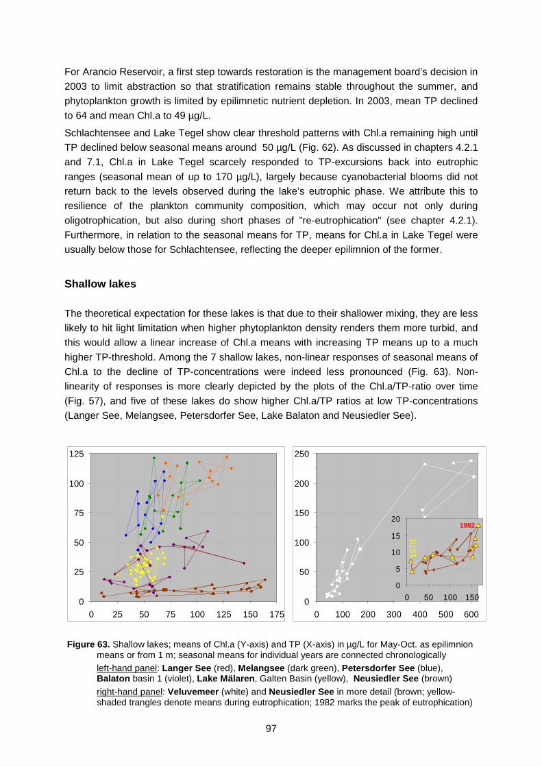
97

For Arancio Reservoir, a first step towards restoration is the management board’s decision in 2003 to limit abstraction so that stratification remains stable throughout the summer, and phytoplankton growth is limited by epilimnetic nutrient depletion. In 2003, mean TP declined to 64 and mean Chl.a to 49 µg/L.

Schlachtensee and Lake Tegel show clear threshold patterns with Chl.a remaining high until TP declined below seasonal means around 50 µg/L (Fig. 62). As discussed in chapters 4.2.1 and 7.1, Chl.a in Lake Tegel scarcely responded to TP-excursions back into eutrophic ranges (seasonal mean of up to 170 µg/L), largely because cyanobacterial blooms did not return back to the levels observed during the lake’s eutrophic phase. We attribute this to resilience of the plankton community composition, which may occur not only during oligotrophication, but also during short phases of "re-eutrophication" (see chapter 4.2.1). Furthermore, in relation to the seasonal means for TP, means for Chl.a in Lake Tegel were usually below those for Schlachtensee, reflecting the deeper epilimnion of the former.

Shallow lakes

The theoretical expectation for these lakes is that due to their shallower mixing, they are less likely to hit light limitation when higher phytoplankton density renders them more turbid, and this would allow a linear increase of Chl.a means with increasing TP means up to a much higher TP-threshold. Among the 7 shallow lakes, non-linear responses of seasonal means of Chl.a to the decline of TP-concentrations were indeed less pronounced (Fig. 63). Non-linearity of responses is more clearly depicted by the plots of the Chl.a/TP-ratio over time (Fig. 57), and five of these lakes do show higher Chl.a/TP ratios at low TP-concentrations (Langer See, Melangsee, Petersdorfer See, Lake Balaton and Neusiedler See).

Figure 63. Shallow lakes; means of Chl.a (Y-axis) and TP (X-axis) in µg/L for May-Oct. as epilimnion

means or from 1 m; seasonal means for individual years are connected chronologically left-hand panel: Langer See (red), Melangsee (dark green), Petersdorfer See (blue), Balaton basin 1 (violet), Lake Mälaren, Galten Basin (yellow), Neusiedler See (brown) right-hand panel: Veluvemeer (white) and Neusiedler See in more detail (brown; yellow-shaded trangles denote means during eutrophication; 1982 marks the peak of eutrophication)

0

25

50

75

100

125

0 25 50 75 100 125 150 1750

50

100

150

200

250

0 100 200 300 400 500 600

0

5

10

15

20

0 50 100 150

1982

1970

0

5

10

15

20

0 50 100 150

1970

1982

98

Veluvemeer covered the widest range of TP-concentrations and showed the most pronounced response of phytoplankton (white curve in Fig. 63): TP-means dropped from 600 µg/L in the early 1980s, first to levels around 100 µg/L by the mid-1990s. While TP-means ranged between 400 and 600 µg/L, seasonal means of Chl.a scattered widely in the range between 150 and 230 µg/L, but below 400 µg/L they followed seasonal means of TP almost linearly. A further decline to seasonal TP means to levels of 40-90 µg/L occurred in the mid 1990s through a “top-down” effect, when – without change of the external load – levels of chlorophyll-a suddenly dropped to around 10 µg/L. This is attributed to a reduction of the bream population (a commercial bream fishery started in the beginning of the 1990s). This allowed zebramussels to return, which reduced the phytoplankton density by their high filtration activity – a “top-down” food-chain effect of grazing (Lammens et al. 2004).

The three lakes in Brandenburg, Germany – i.e. Langer See (red curve) Melangsee (green curve) and Petersdorfer See (blue curve) – have similar depths (Zmax 3.3-4.0 m; Tab. 3) and are part of an interconnected system of lakes. Their seasonal means for Chl.a and TP cluster and overlap, though in different parts of the TP-range: Langer See just scarcely reached TP-concentrations low enough to potentially limit phytoplankton biomass; the smallest of the three – Melangsee – showed more scatter than response; and envelope curves envisaged around the data for Petersdorfer See would show a rather steep relationship between means of TP and Chl.a. At TP >90 µg/L the 8 data points suggest the beginning of a plateau: six means for Langer See and one mean for Melangsee are below a 1:1 ratio (Fig. 63). Compared to the other lakes, their Chl.a means are very high in relation to their TP means, i.e. they use the resource P extremely efficiently: at TP means of 90-30 µg/L their Chl.a/TP-ratios are rarely much below 1 and many are well above 1 (Fig. 57). Nixdorf et al. (2009) explain this high resource use efficiency with species composition: These shallow lakes are dominated by filamentous cyanobacteria, during their eutrophic phase chiefly by Planktothrix agardhii, with a shift to more delicate Oscillatoriales and to Nostocales as TP-levels declined. These taxa use TP very effectively and stabilise high levels of plankton biomass, so far keeping the systems resilient against a switch to macrophyte dominance.

The TP decline in the Galten Basin of Lake Mälaren (yellow curve in Fig. 63) was in a similar range as for Petersdorfer See, and while in both lakes seasonal mean Chl.a-concentrations show a similar slight decline, they were at much lower levels in Lake Mälaren, probably reflecting its deeper mixing.

The Chl.a response to declining seasonal means of TP-concentrations Lake Balaton (violet, Fig. 63) is also not linear, i.e. at TP-means above 100 µg/L the curve flattens out, with seasonal means both for Chl.a and for TP varying widely. Once TP-means were clearly below 40 µg/L, seasonal means for Chl.a remained below 25 µg/L (Tátrai et al., 2008). Light limitation is pronounced in this very shallow, large and wind-exposed lake: it is strongly influenced by its high mineral turbidity: even low wind speeds in the range of 2-3 m/s resuspend the loose uppermost sediment layer. The development of the phytoplankton community therefore is highly dependent on time patterns (frequency and duration) of calm conditions. If – in addition to the mineral turbidity – phytoplankton biomass in the range above 30 µg/L Chl.a adds substantial further shading, light limitation is likely. Interestingly, a TP-increase back up to 75 µg/L did not induce a Chl.a-response back up to previous levels –

99

a phenomenon similar to the observations from Lake Tegel and explicable only by a more detailed analysis, particularly of phytoplankton species composition for signs of resilience (i.e. inter-annual stability of communities), but also of hydrophyisical patterns.

Light limitation due to suspended sediment is yet more pronounced in Neusiedler See, and seasonal means of Chl.a therefore are extremely low in relation to TP (Fig. 63, brown, right-hand curve; see also Dokulil 1994). Dokulil et al. (2006) propose a critical ratio of 3:1 for TP:Chl.a for lakes with high turbidity and/or macrophyte dominance, and both characteristics apply to Neusiedler See. In the course of this large shallow lake’s eutrophication during the late 1970s, TP concentrations increased dramatically (Fig. 63, right-hand panel, yellow triangles), from a seasonal mean of 10 µg/L in 1970 to a mean of 164 µg/L by 1982. Chl.a means first showed little response to eutrophication and appeared to hit an upper limit around 10 µg/L, but then increased further – up to 18 µg/L by 1982. Thus, while resilience has primarily been postulated for lake restoration, Neusiedler See appears to show this phenomenon during eutrophication rather than during oligotrophication. In contrast to this resilience pattern during eutrophication, in the course of re-oligotrophication the means for Chl.a scattered more widely around the TP decline: in some years they were well below those of the eutrophication phase and in other years, they were higher. Again, for an explanation the analysis of phytoplankton community composition in relation to other biota and to the hydrophysical conditions would be necessary.

Summary and conclusions for future studies A key outcome of this 19-lake analysis is that non-linear responses of phytoplankton biomass to declining TP concentrations are indeed common: 12 lakes showed pronounced non-linear responses, and among these, 5 stratified and 2 shallow lakes showed clear TP thresholds above which TP did not control seasonal means of Chl.a concentrations (Table 4). Others showed resilience against Chl.a-reduction in spite of a significant range of TP-reduction – e.g. Wahnbach Reservoir in the range of mean TP-concentrations declining from 35 to 20 µg/L and Lake Geneva as TP declined from 45 to 25 µg/L. Yet others have not moved through a sufficiently large span of TP-concentrations to show such thresholds (e.g. Lago Maggiore, Petersdorfer See, Melangsee and the Galten Basin of Lake Mälaren). Furthermore, some non-linear response patterns are also due to other factors such as changes in grazing pressure, both in deep stratifying lakes (e.g. in Lago Maggiore, Lake Geneva) and in shallow lakes (e.g. Veluvemeer).

For the shallow lakes the plateaus of Chl.a over TP during their highly eutrophic phases are not as pronounced – rather, in the range of high TP concentrations their seasonal means of Chl.a against TP zig-zag or spiral between higher and somewhat reduced levels, with Chl.a following TP only in some years. As their mean TP-concentrations declined further through the lower concentration range, means of Chl.a follow TP more closely. Contrary to the early results published by Sas (1989), for deeper stratified lakes the longer time series now available show markedly less variability than those for the shallow lakes, both when comparing responses between lakes and when analysing time series for individual lakes.

100

Table 4. Total phosphorus (TP)-thresholds for a phytoplankton response, estimated from plots of seasonal means (epilimnion or surface) for Chlorophyll-a against those for TP

Lake Mixing depth

TP threshold (seasonal means)

Maximum seasonal mean

Chl.a in the eutrophic phase

m µg/L µg/L

Lake Constance 5-20 ~ 20 10

Lake Mälaren (Ekoln Basin) 8-10 ~ 50 27*

Lake Tegel 5-8 ~ 50 62

Scharmützelsee 4-6 ~ 35 34

Schlachtensee 3-5 ~ 35 98

Lake Balaton 2.4 ~ 30 59

Veluvemeer 1.3 ~ 400 240 * 60 µg/L in an exceptional year with a cyanobacterial bloom

A hypothesis to test with the data showing TP-thresholds for the Chl.a- response was that in water-bodies with deeper mixing (of the epilimnion or in the case of shallow lakes of the whole lake) TP-thresholds would be lower than in shallow water-bodies or such with a shallow epilimnium. The thresholds that were identifiable in the 7 lake plots show some confirmation of this hypothesis: in the often deeply mixed epilimnion of Lake Constance, the TP threshold for the restoration response was lowest. Lake Mälaren (Ekoln Basin), Lake Tegel, Scharmützelsee or Schlachtensee which have shallower epilimnia showed a higher TP-threshold and attained higher maximal seasonal means of Chl.a (Tab. 4). At the other end of the scale, the very shallow Veluvemeer showed an extremely high TP threshold and an extgremely high maximum seasonal mean for Chl.a. The low TP-threshold of Lake Balaton does not fit into the picture, probably because its high mineral turbidity prevents higher phytoplankton density even when TP-levels would offer a higher carrying capacity. The data from most of the water-bodies for which we cannot discern any threshold patterns do fit into the overall picture of Chl.a means in relation to TP means. Extremes such as Arancio Reservoir or Neusiedler See highlight the importance of factors such as reservoir draw-down or mineral turbidity.

All in all, the results confirm that valuable data sets are now available for modelling approaches to quantify TP thresholds in relation to hydrophysical parameters that determine mixing characteristics and thus light limitation. This would require modelling the carrying capacity in terms of available under-water photon flux in relation to that in terms of nutrients. The former would need to include the impact not only of turbidity due to particles and dissolved substances, but also the impact of patterns of wind-induced mixing. Such a model could define a corridor of response, within which biotic interactions further define phytoplankton levels.

101

A striking response phytoplankton biomass yields or efficiency of use of P as resource to the decline of TP-concentrations is that for most of the 19 water-bodies, Chl.a/TP-ratios increased as TP declined, reaching maxima in the TP-range of 30-60 µg/L, with some lakes switching to lower Chl.a/TP-ratios again once TP-concentrations become very low (Fig. 57). This non-linearity may be caused by several mechanisms, e.g. shifts of TP allocation between phytoplankton and other suspended particles, species shifts within the phytoplankton towards those which produce more Chl.a per unit biomass or persistence of Oscillatoriales and Nostocales. Additionally, the depths at which large shares of phytoplankton populations are located may shift as lakes get clearer, and in consequence the epilimnion samples behind these data may no longer fully represent the phytoplankton population. For biotic resilience against change – both in eutrophication and in oligotrophication – the stability of plankton and predator communities may be important. Also, in shallow lakes P-partitioning between phytoplankton and macrophytes may stabilise responses (see Scheffer’s (1993) alternative state hypothesis which proposes sudden shifts from plankton-dominance to macrophyte dominance). Early lake restoration research postulated biotic resilience against responses to declining TP concentrations to be an important impediment against restoration success (Sas 1989). Hysteresis effects would imply that during oligotrophication, in relation to a given TP concentration, phytoplankton biomass will linger at higher levels than during eutrophication.

In our data set, two lakes show the opposite of hysteresis, i.e. pronounced resilience also during eutrophication – Neusiedler See in the mid 1970s and Lake Tegel during a transient several-year re-eutrophication phase from 1998 to 20034

The identification of such patterns would have substantial management implications. An example is the need for further measures (such as fish stock management) in order to accelerate the biological response to reduced TP-concentrations – an option that may push a lake over a decisive TP-threshold: For shallow lakes, Jeppesen et al. (2007b) report that the widely discussed alternative states actually are not often observed in practice, probably because each state is less stable than originally assumed. Rather, these authors emphasise that northern temperate lakes often shift gradually, with the reduction of Chl.a concentrations following that of TP-concentrations quite directly. In consequence, a few years of patience may be more adequate than additional measures to push the biotic system towards a faster response. For such decisions, lake restoration planning would benefit from a systematic evaluation of restoration data that identifies situations causing resilience phenomena, their

. The data for both lakes suggest that resilience may last for 3-4 years, but then give way with a sudden shift to abruptly higher or lower Chl.a means at only slightly changed TP concentrations. It may be worthwhile to scrutinize such data sets for identifying resilience mechanisms and factors that trigger change of previously stabilising biotic interactions. In the context of a renewed restoration response evaluation, in-depth analysis of the biotic interactions would be important in order to identify the key drivers behind their specific non-linear or threshold response patterns.

4 As discussed in chapter 5, for Lake Tegel we postulate that the reason why Microcystis blooms did

not re-appear during the re-eutrophication years is that smaller summer populations lead to fewer colonies overwintering on the sediment and thus to lower inocula for the next vegetation period. This would imply that the build-up of hypertrophic bloom levels may require a few years – a hypothesis that remains to be validated by studies of sediment population sizes.

102

magnitude and stability, towards developing planning tools to assess the added value of additional measures.

A further cause for delayed or erratic responses to declining TP may be an occasional role for N-limitation at high TP-levels (e.g. in Lake Geneva; see also Sas 1989 for examples): Complementary to the above-discussed evidence that nitrogen is rarely more important than phosphorus for direct limitation of phytoplankton biomass, indirect effects have been proposed. One – particularly relevant in clear lakes with sufficient light for substantial nitrogen fixation – is the impact of nitrogen limitation on species composition by favouring nitrogen fixing cyanobacteria, as this may strongly influence the community structure responses to trophic change. Another is the detrimental impact of excess nitrogen observed on aquatic macrophytes: Jeppesen et al. (2007b) show that the growth of submerged aquatic plants diminishes at moderately high TP-concentrations if nitrogen concentrations are above 1-2 mg/L, thus suppressing the supporting effect of macrophyte growth for trophic recovery of shallow lakes. In consequence, although the authors emphasise that phytoplankton proliferation is best controlled by reducing P-concentrations, they propose the role of N to be more significant than commonly assumed. An in-depth evaluation of lake restoration data should therefore include nitrogen concentrations.

In summary, our attempt in OLIGO to describe and categorise restoration response patterns shows the following outcomes: Response patterns are very clear for many lakes, particularly deep stratified ones, that they differ between lake types, and that data series now are sufficiently long for the analysis of phases of resilience, as they now include phases following resilience. Many Chl.a responses tightly follow TP changes for the lower part of the TP range. Models predicting the phytoplankton response to the decline of TP could now be built with more differentiation between lake types, in particular by including mixing depth as key determinant of underwater light availability, but also including modules for other biota and for effects of nitrogen on species composition. Such models have the potential to achieve a substantially lower uncertainty than the Vollenweider regression.

In conjunction with the progress in phytoplankton ecology and lake ecosystem modelling, a new project targeting the development of models to predict restoration responses has very good success chances. Such a project can draw on the concept outlined by Sas et al. (1989) and should include the identification of TP threshold mechanisms as well as the threshold levels for different lake types. For this aim, it needs to take the above-mentioned diversity of potential mechanisms for non-linear responses to reduced TP-levels into account, i.e. teasing out patterns that may be generalised requires an in-depth understanding of each lake and data set. A project “Sas Reloaded” would benefit from co-ordination by a limnologist with modelling experience and from intensive collaboration with the scientists familiar with their lake data.

103

7.3 Mechanistic Phytoplankton Model for Schlachtensee Inke Schauser Alex Elliott, Stephen Thackeray

During late 2005 and 2006, OLIGO collaborated with Dr. Alex Eliot from the Centre for Ecology & Hydrology, Lancaster, U.K. to attempt to run their lake phytoplankton community computer model PROTECH (Phytoplankton RespOnses To Environmental CHange) with selected years of Schlachtensee data to understand the relationships between the nutrient cycle and the phytoplankton biomass better and to explain the succession pattern in the phytoplankton composition.

We chose PROTECH as, among the few mechanistic, i.e. process-driven phytoplankton models currently available, it is the most advanced, as it includes many species, whereas others depict only few species or groups (see outcomes of the workshop on Perspectives of Lake Modelling Towards Predicting Reactions to Trophic Change”; Schauser et al. 2008). Furthermore, a focus of work in 2005 and 2006 was collaboration with the EU project CLIME, particularly the Swedish Meteorological and Hydrological Institute in Nörrköping, Sweden. This provided the opportunity to understand and apply the hydrodynamic model PROBE (Svensson, 1998; Sahlberg, 2003) at Schlachtensee to model temperature regimes, vertical stratification and ice formation on a daily scale. Whilst PROTECH also simulates the physical structure of the lake, it makes no allowance for the formation of ice. Thus, PROBE was used to provide the complete physical structure. This link between the two models has been successfully made before (Elliott et al. 2007).

PROTECH predicts the daily growth of select phytoplankton species using morphologically dependent growth rates. The fundamental core of the biological component of PROTECH is the basic state variable equation determining the daily change in the Chlorophyll-a concentration (X) of each algal species:

[2] ∆X/∆t = (r’ – S – G –D).X mg m-3 d-1

where r’ is the growth rate defined as a proportional increase over 24 hours, S is the losses due to settling out of the water column, G is the loss due to grazing (species > 50 µm are not grazed) and D is the loss due to dilution. The growth rate (r’) is further defined by:

[3] r’ = min{r’(θ,I), r’P, r’N, r’Si} d-1

where r’(θ,I) is the growth rate due to temperature and daily photoperiod and r’P, r’N, r’Si are the growth rates determined by phosphorous, nitrogen and silicon concentrations.

Simulating Schlachtensee 1988

We chose the data set from Schlachtensee 1988 for the trial run because of the high sampling frequency in that year, i.e. good temporal resolution of the phytoplankton data. PROBE accurately simulated the annual temperature and stratification regime and was used to drive the PROTECH biological simulation. This simulation matched the observed general

104

seasonal changes in total chlorophyll very well in 1998, with the exception of early spring (Fig. 64) but was less accurate at reproducing the exact timing of the observed taxonomical changes (Fig. 65). It did, however, reflect the observed successional pattern of dominance of diatoms others diatoms + cyanobacteria.

Figure 64. Comparison between observed (X) and simulated (red line) for total chlorophyll (mg m-3) in Schlachtensee 1988.

However, an important modifi-cation was necessary to pro-duce this simulation, namely the model was run with phosphorus “added” to the hypolimnion (i.e. water-body deeper than 4.5 m) between 9th June and 28th August. This allowed for the observed increase of the in-lake phosphorus concentration due to suspected internal release of phosphorus from the sediments during this period, which is a process not yet simulated in PROTECH, but indeed ob-served in Schlachtensee, where hypolimnetic P concentrations increase from around 20 µg L-1 before thermal stratification to around 100 µg L-1 during the summer due to release from the sediments (see chapter 4.2.1). Figure 65. Comparison between observed and simulated

community taxa composition in Schlachtensee 1988 X-axis: days of the year

0%

20%

40%

60%

80%

100%

55 83 118 139 154 167 195 209 223 237 258 272 300

OthersCyanobacteriaDiatoms

0%

20%

40%

60%

80%

100%

55 83 118 139 154 167 195 209 223 237 258 272 300

OthersCyanobacteriaDiatoms

PROTECH

Observed

0

2

4

6

8

10

12

14

16

18

20

0 50 100 150 200 250 300

Day

Chl

orop

hyll

(m

g/

105

The results show that PROTECH is capable of simulating the general pattern of chlorophyll change in the lake throughout most of the year (Fig. 64). An approximate simulation of the observed successional sequence of taxa dominance by major groups, as achieved in this study, is the least that any phytoplankton model should achieve. The differences in taxo-nomic composition between the observed data and the result of the PROTECH simulation was expected, particularly for timing (Fig. 65), as replicating precise species dynamics is very challenging.

However, the poor match between observed data for chlorophyll-a and the simulation in high winter/early spring just after the ice covered period shows that PROTECH cannot yet simulate large amounts of biomass under these relatively light poor and cold conditions. Further work is warranted to understand how phytoplankton can produce such large amounts of net growth under these very limiting conditions.

106

7.4 Steps towards a statistical model to predict phytoplankton responses to changes in trophic state Ingrid Chorus and Verena Niesel,

with data provided by Kirsten Christoffersen, Jutta Fastner, Eberhard Hoehn, Liisa Lepistö, Svantje Koch, Antje Köhler, Rainer Koschel, Rainer Kurmayer, Ernst Nusch, Helmut Rönicke, Petra Visser, Norbert Walz and Hartmut Willmitzer

The model PROTECH used for the simulation described in Chapter 7.3 is based on growth rate data for a range of species and conditions, interlinking them with mechanistic functions (Reynolds et al. 2001). The ecological concept behind this modelling approach (described in Reynolds 1997) is to characterise specific habitats and their typical representatives with patterns of growth rates in relation to environmental variables. Additionally, Reynolds et al. (2002) published a widely used allocation of characteristic phytoplankton taxa to a range of “functional associations” or habitats. This “functional associations concept” serves as verbal model to describe which species to expect under which conditions. Padisák et al. (2009) assessed the widespread – in fact global – application of this verbal model for the characterisation of phytoplankton associations, resulting in a tightening of habitat descriptions and taxa allocations, as well as in the description of further habitats and some of their typical inhabitants.

Reynolds et al. (2002) explicitly invite users to develop the functional associations or habitat templates further, emphasing the need to ground such development on a robust data basis. While growth rates are the most immediate response to a combination of environmental variables, their outcome – i.e. the size of the standing stock – will also reflect this response unless the environmental variables substantially change faster than the population can respond. Therefore, field data on the occurrence and biovolumes of taxa which are characteristic of habitats should provide a basis for further developing the concept of phytoplankton functional associations. Complementary to growth rate data from the laboratory, they can capture the combination of conditions impacting on phytoplankton population sizes in natural situations. A statistical evaluation of the occurrence of taxa in relation to environmental variables should therefore contribute to developing and validating the habitat descriptions currently so widely used. In the short term, a model predicting the likelihood of taxa to occur – potentially differentiating by categories of biomass levels – on a statistical basis may be an alternative in face of the limitations of current mechanistic or functional modelling of phytoplankton populations discussed in Chapter 7.3 and at the OLIGO modelling workshop “Perspectives of Lake Modelling Towards Predicting Reactions to Trophic Change” (Schauser, ed. 2008). In the longer term, these complementary approaches might be fruitfully merged.

To these aims, we pursued a statistical approach to modelling species occurrence. This was first developed with data from reservoirs in middle-range mountain areas of Germany (Niesel et al. 2007). Here, we use this “Phytoplankton Data Base”, expanding the approach towards a semi-quantitative analysis of the likelihood of phytoplankton taxa to occur, and we compare the results to changes in patterns of occurrence in Schlachtensee and Lake Tegel in the

107

course of restoration. Additionally, for analysing the likelihood of cyanobacterial occurrence, we built a larger “Cyanobacteria Data Base” by combining the Phytoplankton Data Base with data bases from two other projects5

Our statistical approach first defines categories for each parameter to be studied (e.g. five for total phosphorus, ranging from < 10 to > 90 µg/L, Fig. 66) and assesses the frequency distribution of all samples in the data base across these categories. To this it then compares the frequency distribution of samples containing a given taxon across the same categories. With a Chi² test it assesses whether the likelihood of the taxon to occur in the category of the parameter is significantly enhanced or reduced, or whether the relative frequency of the taxon’s occurrence in that category is not significantly different from that of all samples.

(which contain biovolume data for total phytoplankton and cyanobacteria, but do not detail the other phytoplankton taxa). We gratefully acknowledge those who originally had provided these data in the contexts of all three earlier projects (see Tab. 5 below) for their permission to re-use them here.

Figure 66. Example of frequency ratios for a given taxon (here Aphanizomenon spp. at biovolumes

>0.5 mm³/L) in different categories of a given parameter (here TP) calculated as: % samples with the taxon in the category % of all samples in the data base in the category

Legend for significance of frequency ratio according to Chi² test results <: none or extremely rare -: significantly reduced n: no significant difference +: significanty elevated

The example given in Fig. 66 illustrates this approach: data for TP and phytoplankton were available for 1928 samples. These spread across the 5 categories of TP-concentrations as shown by the grey solid bars. 491 of these 1928 samples contained Microcystis spp., and the hatched bars show their distribution across the 5 categories of TP-concentrations. Differences in the frequency of occurrence of both sample sets are significant for the TP-categories < 10 µg/L (underrepresentation) as well as for the categories >25-50, >50-90 and

5 Peptides in Cyanobacteria (PEPCY) and Toxic Cyanobacteria in German Water-Bodies.

0

20

40

60

80

100

< 10 10 - 25 > 25-50 > 50-90 > 90

TP concentration categories [µg/L]

% s

ampl

es in

TP

cat

egor

y

0

1

2

3

4

5

f

ti

% of all samples (n = 1928)% with Aphanizomenon > 0.5 mm³/L (n=87)frequency ratio

% s

ampl

esin

TP

cate

gory

< - n n +

frequ

ency

ratio

0

20

40

60

80

100

< 10 10 - 25 > 25-50 > 50-90 > 90

TP concentration categories [µg/L]

% s

ampl

es in

TP

cat

egor

y

0

1

2

3

4

5

f

ti

% of all samples (n = 1928)% with Aphanizomenon > 0.5 mm³/L (n=87)frequency ratio

% s

ampl

esin

TP

cate

gory

< - n n +

frequ

ency

ratio

% s

ampl

esin

TP

cate

gory

< - n n +

frequ

ency

ratio

108

>90 µg/L (overrepresentation), indicating water bodies with TP-concentrations above 25 µg/L to be a favourable habitat for Microcystis spp. while their likelihood to occur is reduced at TP < 10 µg/L.

We then repeat this analysis for different biovolume subsets of the samples containing the taxon, i.e. with all samples containing elevated (>0.1 mm³/L) and all samples containing high (>0.5 mm³/L) Microcystis-biovolumes. The outcome focuses more tightly on the conditions under which populations of the taxon are likely to proliferate. Tab. 6 (below) summarises such results for 6 cyanobacterial taxa at 3 levels of biovolume, in relation to 3 general water-body characteristics as well as to the status of 5 environmental variables at the time of sampling.

For a quantitative measure of under- and over-representation of a given taxon in a category of a parameter, we used the ratio of the percentage of samples with the taxon to the percentage of all samples of the data base in that category and termed this the “frequency ratio”. In the example shown in Fig. 66, only 6 % of all samples with Microcystis spp. occurred at TP concentrations < 10 µg/L, while 26% of all samples in the data base were in this category. Therefore, the frequency ratio for this taxon to occur at TP < 10 µg/L is only about 0.2 (i.e, 20%; solid pink bar), while it is almost 2-fold enhanced at TP > 90 µg/L (solid green bars). Ratios close to 1 show that the taxon occurs in the given category at a rate similar to the occurrence of all phytoplankton. Ratios quite different from 1 usually prove significant according to the Chi² test (with the number of samples in the category determining the threshold for significance). This approach is similar to evaluating election results across age groups: e.g. if 30% of the citicens of Germany vote for party X, with 40% of the age group of 18-30 year old citizens and only 20% of the age group of 60-70 year old citicens vote for this party, the frequency ratio of young people to vote for party X would amount to 40/30, i.e. 1.33, while that of the old people would amount to 20/30, i.e. 0.66. (Also, we may conclude the likelihood for support from the young voters to be twice as high as from the old ones).

However, the quantitative characterisation of occurrence frequencies with ratios of percentages is highly sensitive to the sample selection in the data-base. The larger the sample numbers in each category, the more meaningful this quantification. Our rather small data bases currently allow only a preliminary sketch of such results. We see their current value primarily in comparing the sensitivity of taxa to specific environmental conditions, while they do not (yet) serve to predict the likelihood of a taxon to occur. Therefore, here we report this quantitative comparison only for the parameters trophic state and TP concentrations, as the impact of these parameters on species occurrence is a focal question of OLIGO. The aim is to test whether this approach to quantification of likelihoods of occurrence is worth pursuing in a future project.

The samples in the data bases are not evenly spread across geographic regions, time, water-body types, environmental parameters or their categories. A specific feature of this statistical approach is maximum exploitation of such unevenly distributed data, as the case-by-case evaluation for each parameter and each taxon does not require homogeneous distributions. Our criterion for choosing the taxa to analyse was their occurrence with suffi-cient frequency in the data bases and in at least one of the two lakes of the OLIGO project.

109

Data bases for the analysis: The Cyanobacteria Data Base includes water bodies in Fin-land, Germany, Austria, Denmark, the Netherlands and Italy whereas the Phytoplankton Data Base is smaller and includes water bodies only from Germany. Tab. 5 (below) gives an overview of the water bodies included in both data bases. Both contain data on the bio-volumes of the taxa analysed as well as on abiotic parameters characterising phytoplankton habitats. Here we analyse them with respect to 8 parameters, some of which are interrelated, i.e. seasonality, temperature, mean depth, thermal stratification, concentrations of total phosphorus (TP), trophic state (as characterised by the data providers), transparency and pH. Fig. 67 shows these parameters together with the categories analysed for each parameter, the total number of samples with data on the parameter and their frequency distribution of the samples across its categories.

The Phytoplankton Data Base contains 1519 samples obtained between 1993 and 2000 from 20 middle-range (140-780 m altitude) mountain reservoirs in Saxonia, Thuringia and south-ern Germany. Besides data for Schlachtensee and Lake Tegel, it includes data from 18 water-bodies first analysed in the project: “Statistical modelling of phytoplankton occurrence in German middle-range mountain reservoirs” (BMBF Grant Number 02 WT 9852/7; Niesel et al. 2007). These were contributed by H. Willmitzer (Thüringer Fernwasserversorgung), R. Sudbrack (Landestalsperrenverwaltung des Freistaates Sachsen) and the Water Supply Kleine Kinzig in collaboration with the Limnology Laboratory of E. Hoehn. They are well harmonised through regular meetings of the laboratories involved for comparing methods of determination and quantification.

Of these 20 water-bodies, 5 were classified as ‘oligotrophic’ by the sample providers, while 7 ranged as ‘mesotrophic’ and 8 as ‘eutrophic’ (including hyper- or polytrophic). As sample numbers vary between water-bodies, this distribution of water-bodies is only partially reflec-ted by the distribution of samples over trophic states: more than half of the samples originate from mesotrophic water-bodies, including a fair share of samples with TP-concentrations below 10 µg/L at the time of sampling (TP is <10 µg/L in 44% of all samples; Fig. 7.2). Less than ¼ of all samples contained more than 25 µg/L TP, and this is reflected by sample distri-bution in relation to water transparency: only ¼ of all samples were from conditions with Secchi disc readings of less than 2 m. 18 of the water-bodies developed thermal stratification during summer, while 2 are shallow and polymictic. 2 are acidic, 18 are not. The samples are distributed fairly evenly across all four seasons, with a slightly lower share taken in winter and few taken at water temperatures >16°C (Fig. 7.2).

The Cyanobacteria Data Base includes 3231 samples obtained between 1993 and 2004 from 210 water-bodies (Tab. 5). It is about twice as large as the Phytoplankton Data Base because it includes those data as well as data from two further projects: 542 samples from Germany collected in the project “Cyanotoxins – Occurrence, Causes Consequences” (BMBF, Grant Number 0339547, Wiedner et al. 2001), 743 samples from the Netherlands, Denmark, Austria, Germany and Italy collected in the project ‘”PEPtides in CYanobacteria” (PEPCY 2007, EU Contract Number QLK4-CT-2002-02634) as well as 427 further samples6

6 without an additional 227 samples from these 2 lakes in the BMBF and PEPCY project data bases

from Lake Tegel and Schlachtensee studied in OLIGO. Some water-bodies were sampled

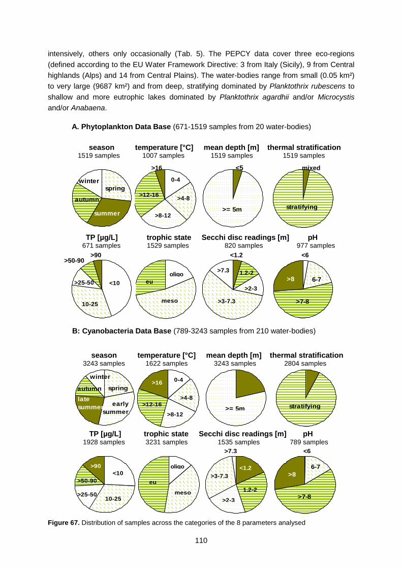
110

intensively, others only occasionally (Tab. 5). The PEPCY data cover three eco-regions (defined according to the EU Water Framework Directive: 3 from Italy (Sicily), 9 from Central highlands (Alps) and 14 from Central Plains). The water-bodies range from small (0.05 km²) to very large (9687 km²) and from deep, stratifying dominated by Planktothrix rubescens to shallow and more eutrophic lakes dominated by Planktothrix agardhii and/or Microcystis and/or Anabaena.

A. Phytoplankton Data Base (671-1519 samples from 20 water-bodies)

B: Cyanobacteria Data Base (789-3243 samples from 210 water-bodies)

Figure 67. Distribution of samples across the categories of the 8 parameters analysed

TP [µg/L] trophic state Secchi disc readings [m] pH 671 samples 1529 samples 820 samples 977 samples

spring

early summer

winter

autumnlate summer >= 5m

6-7

>7-8

>8

>4-8

>16

>8-12

0-4

>12-16 stratifying

<10

10-25>25-50

>50-90

>90 oligo

meso

eu

>2-3

>3-7.3

1.2-2

<1.2

spring

summer

winter

autumn>= 5m

6-76 7

>7-8

>8<10

10-25

>25-50oligo

meso

eu

>4-8

>8-12

0-4

>12-16

stratifying

>2-3

>7.3

>3-7.3

1.2-2

>50-90 >90 <1.2 <6

mixed >16 <5

season temperature [°C] mean depth [m] thermal stratification 1519 samples 1007 samples 1519 samples 1519 samples

season temperature [°C] mean depth [m] thermal stratification 3243 samples 1622 samples 3243 samples 2804 samples

<6 >7.3

TP [µg/L] trophic state Secchi disc readings [m] pH 1928 samples 3231 samples 1535 samples 789 samples

111

The distribution of samples across the categories of the abiotic parameters is not fundamentally different between both data bases: While for the parameter ‘season’ it is not directly comparible due to further differentiation between ‚early summer’ and ‚late summer’ in the Cyanobacterial Data Base, the share of samples from winter and spring is only slightly lower than in the Phytoplankton Data Base. For sample distribution across categories of temperature the main difference between both data bases is a larger share of samples collected at temperatures above 16°C in the Cyanobacteria Data Base. We attribute this only partially to a stronger focus of sampling on the summer season in the context of cyanobacterial research: in particular, the data base contains a higher share of samples from shallower lakes situated at lower altitudes which therefore become warmer during summer (Fig. 7.2 B). Further, the Cyanobacteria Data Base contains a somewhat higher share of samples with TP-concentrations above 25 µg/L and from water-bodies classified as eutrophic by the data providers. This is reflected by a higher share of samples from turbid conditions with Secchi-Disc readings < 3 m and of samples with pH > 8 (Fig. 7.2 B).

These differences between both data bases in sample distributions across the categories of parameters should have no impact on the outcome of the statistical analysis of the occurrence of individual taxa because (as discussed above) the assessment is based on case-by-case comparisons of the distribution of samples containing a specific taxon to that of all samples across the categories of each parameter.

Table 5. Water-bodies in the Cyanobacteria Data Set (including those in the Phytoplankton Data Set) and no. of samples per water-body

Legend: eu=eutrophic; me=mesotrophic; ol=oligotrophic; mix=polymictic; stra=stratifying (mono- or dimictic)

Phytoplankton Data Base:

Data from*: no Zmean

m Zmax m

A km²

Droeda G LTV 114 me stra 11.6 38.3 1.3 Bautzen G LTV 46 eu stra 7.1 16.8 Eibenstock G LTV 64 ol stra 20.8 52 3.7 Erletor G TFW 61 me stra 8.6 30.9 0.05 Gottleuba G LTV 96 me stra 17.6 43.6 0.7

Kleine Kinzig G WKK / LBH 238 me stra 22.2 57.3 0.6

Klingenberg G LTV 99 me stra 13.5 32 1.2 Loessau G TFW 72 eu mix 3.2 15.1 0.3 Ohra G TFW 49 ol stra 30 58.5 0.8 Pirk G LTV 25 eu stra 13 13.5 1.5 Poehl G LTV 40 eu stra 15.4 41.5 3.9 Radeburg Reservoir 2 G LTV 5 eu mix 2.3 6.42 2.8

Saidenbach G LTV a 138 me stra 15.8 46.8 1.4 Scheibe G TFW 51 ol stra 8.2 23 0.3 Schmalwasser G TFW 66 me stra 26.9 80.7 0.8 Schwarza G TFW 68 eu stra 14.6 42.5 0.2 Schoenbrunn G TFW 71 ol stra 23.4 66.7 1 Tambach G TFW 43 ol stra 8.9 26.5 5.6

Cyanobacteria Data Base = Phytoplankton Data Base plus:

Data from: no Zmean

m Zmax

M A

km² Arendsee G UfZ 65 eu stra 28.6 48.7 5.1 Biggetalsperre G Ru Vb 1 me stra 20.3 49.5 895 Breiter Luzin G IGB N 32 me stra 25.2 58.5 2.7 Grimnitzsee G IBG B 22 eu mix 3.8 9 7.7 Haussee G IGB N 34 eu stra 6.3 12 1.3 Roetha G LTV 4 mix 1.7 3.9 0.7 Rudower See G UfZ 29 eu mix 4 5 2.1 Schlachtensee G UBA 288 eu mix 4.7 8.5 0.4 Schmaler Luzin G IGB N 34 me stra 14.7 38 1.4 Tegeler See G UBA 366 eu stra 6.6 15.9 4 Tollensesee G IGB N 22 eu stra 17.2 33.2 17.4 Wannsee G UBA 72 eu stra 5.5 10 2.7 Weida G TFW 90 eu stra 10.3 32.5 0.9 Zeulenroda G TFW 83 eu stra 11.7 40.9 2.3 Zeuthener See G ITOX 40 eu mix 1.5 3

Alte Donau A AAS 5 me mix 2.5 6.8 Heustadlwasser A AAS 1 eu mix 1.7 3.3 4.7 Holzöstersee A AAS 8 eu mix 2.3 4.7 0.1 Irrsee A AAS 20 me stra 15 32 3.5

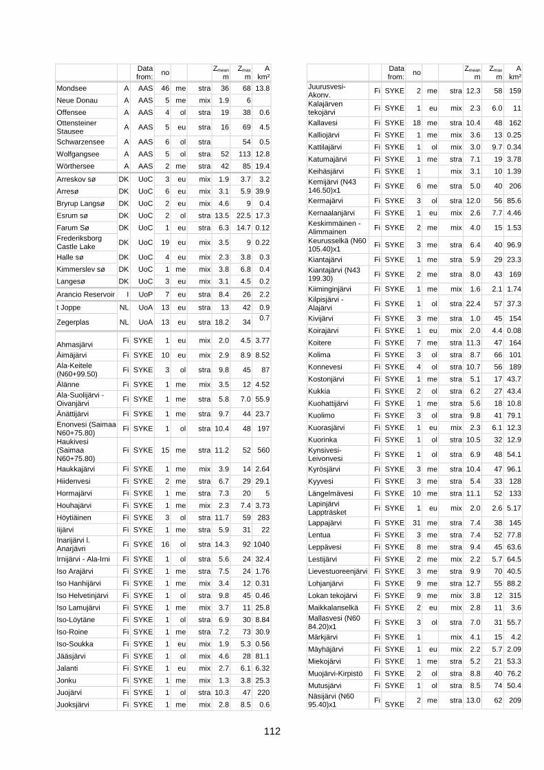
112

Data from: no Zmean

m Zmax

m A

km² Mondsee A AAS 46 me stra 36 68 13.8 Neue Donau A AAS 5 me mix 1.9 6 Offensee A AAS 4 ol stra 19 38 0.6 Ottensteiner Stausee A AAS 5 eu stra 16 69 4.5

Schwarzensee A AAS 6 ol stra 54 0.5 Wolfgangsee A AAS 5 ol stra 52 113 12.8 Wörthersee A AAS 2 me stra 42 85 19.4

Arreskov sø DK UoC 3 eu mix 1.9 3.7 3.2 Arresø DK UoC 6 eu mix 3.1 5.9 39.9 Bryrup Langsø DK UoC 2 eu mix 4.6 9 0.4 Esrum sø DK UoC 2 ol stra 13.5 22.5 17.3 Farum Sø DK UoC 1 eu stra 6.3 14.7 0.12 Frederiksborg Castle Lake DK UoC 19 eu mix 3.5 9 0.22

Halle sø DK UoC 4 eu mix 2.3 3.8 0.3 Kimmerslev sø DK UoC 1 me mix 3.8 6.8 0.4 Langesø DK UoC 3 eu mix 3.1 4.5 0.2

Arancio Reservoir I UoP 7 eu stra 8.4 26 2.2

t Joppe NL UoA 13 eu stra 13 42 0.9

Zegerplas NL UoA 13 eu stra 18.2 34 0.7

Ahmasjärvi Fi SYKE 1 eu mix 2.0 4.5 3.77

Äimäjärvi Fi SYKE 10 eu mix 2.9 8.9 8.52 Ala-Keitele (N60+99.50) Fi SYKE 3 ol stra 9.8 45 87

Älänne Fi SYKE 1 me mix 3.5 12 4.52 Ala-Suolijärvi - Oivanjärvi Fi SYKE 1 me stra 5.8 7.0 55.9

Änättijärvi Fi SYKE 1 me stra 9.7 44 23.7 Enonvesi (Saimaa N60+75.80) Fi SYKE 1 ol stra 10.4 48 197

Haukivesi (Saimaa N60+75.80)

Fi SYKE 15 me stra 11.2 52 560

Haukkajärvi Fi SYKE 1 me mix 3.9 14 2.64 Hiidenvesi Fi SYKE 2 me stra 6.7 29 29.1 Hormajärvi Fi SYKE 1 me stra 7.3 20 5 Houhajärvi Fi SYKE 1 me mix 2.3 7.4 3.73 Höytiäinen Fi SYKE 3 ol stra 11.7 59 283 Iijärvi Fi SYKE 1 me stra 5.9 31 22 Inarijärvi l. Anarjävri Fi SYKE 16 ol stra 14.3 92 1040

Irnijärvi - Ala-Irni Fi SYKE 1 ol stra 5.6 24 32.4 Iso Arajärvi Fi SYKE 1 me stra 7.5 24 1.76 Iso Hanhijärvi Fi SYKE 1 me mix 3.4 12 0.31 Iso Helvetinjärvi Fi SYKE 1 ol stra 9.8 45 0.46 Iso Lamujärvi Fi SYKE 1 me mix 3.7 11 25.8 Iso-Löytäne Fi SYKE 1 ol stra 6.9 30 8.84 Iso-Roine Fi SYKE 1 me stra 7.2 73 30.9 Iso-Soukka Fi SYKE 1 eu mix 1.9 5.3 0.56 Jääsjärvi Fi SYKE 1 ol mix 4.6 28 81.1 Jalanti Fi SYKE 1 eu mix 2.7 6.1 6.32 Jonku Fi SYKE 1 me mix 1.3 3.8 25.3 Juojärvi Fi SYKE 1 ol stra 10.3 47 220 Juoksjärvi Fi SYKE 1 me mix 2.8 8.5 0.6

Data from: no Zmean

m Zmax

m A

km² Juurusvesi-Akonv. Fi SYKE 2 me stra 12.3 58 159

Kalajärven tekojärvi Fi SYKE 1 eu mix 2.3 6.0 11

Kallavesi Fi SYKE 18 me stra 10.4 48 162 Kalliojärvi Fi SYKE 1 me mix 3.6 13 0.25 Kattilajärvi Fi SYKE 1 ol mix 3.0 9.7 0.34 Katumajärvi Fi SYKE 1 me stra 7.1 19 3.78 Keihäsjärvi Fi SYKE 1 mix 3.1 10 1.39 Kemijärvi (N43 146.50)x1 Fi SYKE 6 me stra 5.0 40 206

Kermajärvi Fi SYKE 3 ol stra 12.0 56 85.6 Kernaalanjärvi Fi SYKE 1 eu mix 2.6 7.7 4.46 Keskimmäinen - Alimmainen Fi SYKE 2 me mix 4.0 15 1.53

Keurusselkä (N60 105.40)x1 Fi SYKE 3 me stra 6.4 40 96.9

Kiantajärvi Fi SYKE 1 me stra 5.9 29 23.3 Kiantajärvi (N43 199.30) Fi SYKE 2 me stra 8.0 43 169

Kiiminginjärvi Fi SYKE 1 me mix 1.6 2.1 1.74 Kilpisjärvi - Alajärvi Fi SYKE 1 ol stra 22.4 57 37.3

Kivijärvi Fi SYKE 3 me stra 1.0 45 154 Koirajärvi Fi SYKE 1 eu mix 2.0 4.4 0.08 Koitere Fi SYKE 7 me stra 11.3 47 164 Kolima Fi SYKE 3 ol stra 8.7 66 101 Konnevesi Fi SYKE 4 ol stra 10.7 56 189 Kostonjärvi Fi SYKE 1 me stra 5.1 17 43.7 Kukkia Fi SYKE 2 ol stra 6.2 27 43.4 Kuohattijärvi Fi SYKE 1 me stra 5.6 18 10.8 Kuolimo Fi SYKE 3 ol stra 9.8 41 79.1 Kuorasjärvi Fi SYKE 1 eu mix 2.3 6.1 12.3 Kuorinka Fi SYKE 1 ol stra 10.5 32 12.9 Kynsivesi-Leivonvesi Fi SYKE 1 ol stra 6.9 48 54.1

Kyrösjärvi Fi SYKE 3 me stra 10.4 47 96.1 Kyyvesi Fi SYKE 3 me stra 5.4 33 128 Längelmävesi Fi SYKE 10 me stra 11.1 52 133 Lapinjärvi Lappträsket Fi SYKE 1 eu mix 2.0 2.6 5.17

Lappajärvi Fi SYKE 31 me stra 7.4 38 145 Lentua Fi SYKE 3 me stra 7.4 52 77.8 Leppävesi Fi SYKE 8 me stra 9.4 45 63.6 Lestijärvi Fi SYKE 2 me mix 2.2 5.7 64.5 Lievestuoreenjärvi Fi SYKE 3 me stra 9.9 70 40.5 Lohjanjärvi Fi SYKE 9 me stra 12.7 55 88.2 Lokan tekojärvi Fi SYKE 9 me mix 3.8 12 315 Maikkalanselkä Fi SYKE 2 eu mix 2.8 11 3.6 Mallasvesi (N60 84.20)x1 Fi SYKE 3 ol stra 7.0 31 55.7

Märkjärvi Fi SYKE 1 mix 4.1 15 4.2 Mäyhäjärvi Fi SYKE 1 eu mix 2.2 5.7 2.09 Miekojärvi Fi SYKE 1 me stra 5.2 21 53.3 Muojärvi-Kirpistö Fi SYKE 2 ol stra 8.8 40 76.2 Mutusjärvi Fi SYKE 1 ol stra 8.5 74 50.4 Näsijärvi (N60 95.40)x1 Fi

SYKE 2 me stra 13.0 62 209

113

Data from: no Zmean

m Zmax

m A

km² Näskäjärvi Fi SYKE 1 me mix 2.7 7.9 5.48

Niettaanselkä Fi SYKE 1 me mix 4.2 16 6.04 Nilakka Fi SYKE 2 me stra 5.0 20 169 Onkivesi Fi SYKE 2 eu mix 3.9 15 114 Ontojärvi-Nurmesjärvi Fi SYKE 1 stra 6.7 29 105

Orivesi (Saimaa N60+75.80) Fi SYKE 3 ol stra 14.8 71 601

Oulujärvi (N43 122.20)x1 Fi SYKE 16 me stra 5.6 23 329

Ounasjärvi Fi SYKE 1 me stra 6.6 30 6.93 Pääjärvi Fi SYKE 17 me stra 14.8 85 13.4 Päijänne (kesk. N60+78.10) Fi SYKE 16 me stra 17.4 85 863

Pesiöjärvi Fi SYKE 1 me mix 3.9 15 12.8 Petosenlampi Fi SYKE 1 me mix 3.6 13 0.2 Pielavesi Fi SYKE 2 me stra 6.7 29 110 Pielinen Fi SYKE 13 ol stra 12.6 60 894 Pieni Kuivajärvi Fi SYKE 1 me mix 2.4 6.3 0.36 Pihlajavesi Fi SYKE 3 me stra 5.2 20 20.1 Pihlajavesi (Saimaa) Fi SYKE 1 ol stra 14.2 68 713

Piispajärvi Fi SYKE 1 me mix 3.6 13 12.9 Porttipahdan tekojärvi Fi SYKE 21 me mix 4.4 30 149

Puhosjärvi Fi SYKE 1 me mix 3.0 12 23.7 Punelia Fi SYKE 1 ol stra 5.7 24 8.19 Puruvesi (Saimaa) Fi SYKE 5 ol stra 12.7 60 416

Pusulanjärvi eli Jäämäjärvi Fi SYKE 1 eu mix 4.9 11 2.07

Puujärvi Fi SYKE 1 ol stra 8.3 22 6.45 Puula Fi SYKE 3 ol stra 12.0 60 331 Pyhäjärvi Fi SYKE 10 me stra 5.4 26 155 Pyhäjärvi (N60 77.20) Fi SYKE 1 eu stra 9.1 41 122

Pyhäselkä (Saimaa N60+75.80)

Fi SYKE 3 me stra 13.7 66 361

Rapojärvi-Haukkajärvi Fi SYKE 1 stra 5.8 24 13.2

Rehja-Nuasjärvi Fi SYKE 1 me stra 8.5 42 96.4 Rehtijärvi Fi SYKE 1 eu stra 5.8 24 0.39 Roine (N60 84.20)x3 Fi SYKE 1 me stra 7.4 32 40.4

Sääksjärvi Fi SYKE 1 ol mix 2.8 8.5 2.6 Saimaa Fi SYKE 16 ol stra 16.9 82 1377 Salmijärvi Fi SYKE 1 me mix 4.3 18 3.48 Säyhtee Fi SYKE 1 mix 3.4 12 2.06 Sierramjavri Fi SYKE 1 ol mix 4.7 19 1.08 Siikajärvi Fi SYKE 1 ol stra 5.5 23 0.9 Simijärvi eli Iso-Simi Fi SYKE 1 ol stra 20 43 2.06

Simojärvi (N43 176.00)x2 Fi SYKE 2 ol stra 5.0 27 54.6

Sotkamojärvi Fi SYKE 1 eu mix 4.4 17 2.11 Suininki Fi SYKE 1 me stra 5.8 24 21.7 Suolijärvi Fi SYKE 1 me mix 2.0 12 10.9 Suontee (N60 94.10) Fi SYKE 3 ol stra 8.8 44 88.5

Data from: no Zmean

m Zmax

m A

km² Suuri-Vahvanen Fi SYKE 1 ol stra 5.8 22 1.32 Suvasvesi (N60 81.70) Fi SYKE 2 ol stra 18.2 89 234

Sylkky Fi SYKE 1 mix 4.2 16 1.06 Syysjärvi Fi SYKE 1 mix 3.2 11 1.75 Takkajärvi Fi SYKE 1 me stra 5.4 23 1.13 Tarjanne Fi SYKE 1 me stra 13.4 64 54.9 Tiiläänjärvi Fi SYKE 1 eu mix 4.4 10 2.13 Toisvesi Fi SYKE 1 me stra 19.5 85 29.4 Tuusulanjärvi Fi SYKE 104 eu mix 3.2 10 5.92 Tyräjärvi Fi SYKE 1 me mix 4.0 16 23.9 Ukonvesi (Saimaa) Fi SYKE 1 stra 6.8 29 24.2

Unari Fi SYKE 1 me stra 5.8 24 28.8 Unnukka Fi SYKE 1 me stra 6.6 36 80.5 Urajärvi Fi SYKE 1 me mix 4.4 16 14.1 Vanajavesi (N60 79.40)x2 Fi SYKE 4 me stra 5.5 23 103

Vatianjärvi Fi SYKE 1 me mix 4.1 28 6.12 Veckjärvi Fi SYKE 1 me mix 3.0 9.5 1.89 Vesijärvi Fi SYKE 8 me stra 6.6 40 108 Viinijärvi Fi SYKE 3 me stra 6.1 58 135 Vitträsk Fi SYKE 1 me stra 5.4 22 4.86 Vuohijärvi Fi SYKE 5 ol stra 16.3 76 86.2 Vuokkijärvi Fi SYKE 1 me stra 5.0 24 51.2 Vuosjärvi Fi SYKE 1 me mix 4.2 25 39.8 Ylä-Keitele (N60 99.50) Fi SYKE 1 me stra 12.7 60 79.2

Yli-Kitka Fi SYKE 15 ol mix 4.6 42 237

*Data from:

LTV: State Reservoir Administration of Saxony, R. Sudbrack and S. Koch

TFW: Thuringia Reservoir Supply, H. Willmitzer WKK/LBH: Water Supply Kleine Kinzig and Limnology

Laboratory Hoehn UFZ: Helmholtz Centre for Environmental Research

– UFZ, H. Rönicke RuVb: Ruhr River Basin Management Association, E.

Nusch IGB-N: Leibniz Inst. of Freshwater Ecology and Inland

Fisheries, R. Koschel IGB-B: Leibniz Inst. of Freshwater Ecology and Inland

Fisheries, N. Walz ITOX: Berlin Senate Administration of Health,

Environment & Consumer Protection, Dept. Water Research, Water Management and Geology, A. Köhler

UBA: Federal Environment Agency Germany, J. Fastner, G. Schlag, K. Laskus

AAS: Austrian Academy of Sciences, R. Kurmayer

UoC: University of Copenhagen, K. Christoffersen

UoP: University of Palermo, L. Naselli-Flores UoA: University of Amsterdam, P. M. Visser SYKE: Finnish Environmental Institute, L. Lepistö

114

Table 6. Occurrence of Cyanobacteria in the Cyanobacteria Data Set Legend: + significantly elevated occurrence; – significantly reduced occurrence; < occurrence with < 5% of total number of recordings; n = difference to all samples not significant. Note: for Limnothrix spp., data on pH were available for very few samples only, so no statistical evaluation was possible

in total data set

with Micr.

Chi² result

with Micr.

Chi² result

with Micr.

Chi² result

with Aph.

Chi² result

with Aph.

Chi² result

with Aph.

Chi² result

with Pla.

Chi² result

with Pla.

Chi² result

with Pla.

Chi² result

with Lim.

Chi² result

with Lim.

Chi² result

with Lim.

Chi² result

with Ana.

Chi² result

with Ana.

Chi² result

with Ana.

Chi² result

with Pla.

Chi² result

< 5 m 693 248 + 113 + 76 + 185 + 58 + 43 + 114 + 51 + 40 + 81 + 47 + 35 + 256 - 68 + 44 + 104 +>= 5 m 2550 484 - 183 - 143 - 433 - 80 - 48 - 197 - 50 - 41 - 138 - 46 - 32 - 60 + 26 - 17 - 235 -

stratified 2592 545 n 238 n 169 n 298 - 87 - 56 - 179 n 85 n 69 n 160 - 59 - 44 - 222 + 52 - 30 n 300 nmixed 212 78 + 38 + 32 + 65 + 34 + 27 + 7 n 5 n 4 n 56 + 34 + 23 + 394 - 24 + 14 + 19 n

eu 1544 617 + 295 + 218 + 358 + 126 + 84 + 189 + 101 + 81 + 215 + 93 + 67 + 299 n 86 + 56 + 251 +meso 1264 101 - 0 < 0 < 188 - 12 - 7 - 101 n 0 < 0 < 4 < 0 < 0 < 216 n 4 < 2 < 65 -

oligo 423 11 < 0 < 0 < 68 n 0 < 0 < 19 - 0 < 0 < 0 < 0 < 0 < 92 n 1 < 1 < 22 -

spring 704 37 - 1 < 0 < 35 - 9 - 7 n 35 - 14 n 11 n 74 + 36 + 23 n 21 < 4 < 2 < 47 -early summer 1029 264 n 82 n 54 n 329 + 53 n 31 n 147 + 22 n 17 n 57 n 24 n 21 n 370 + 37 n 25 n 102 nlate summer 736 325 + 190 + 151 + 207 + 70 + 48 + 92 n 48 + 40 + 36 n 18 n 12 n 199 + 51 + 32 + 121 +autumn 412 97 n 23 n 14 n 39 - 6 n 5 n 25 n 14 n 11 n 20 n 10 n 8 n 23 - 2 < 2 < 39 nwinter 362 9 < 0 < 0 < 8 - 0 - 0 < 12 < 3 < 2 < 32 n 5 n 3 < 3 < 0 < 0 < 30 n

< 10 501 28 - 12 - 8 - 72 - 0 < 0 < 29 - 0 < 0 < 2 < 0 < 0 < 100 - 1 < 0 < 26 - 10 - 25 623 129 n 15 - 5 - 164 n 5 - 4 - 91 n 4 - 4 n 7 < 1 < 1 < 186 n 4 - 2 < 43 n> 25-50 302 102 + 30 n 21 n 64 n 12 n 3 n 27 n 7 n 6 n 25 n 10 n 5 n 71 n 8 n 5 n 30 n> 50-90 246 107 + 40 + 24 n 79 n 17 n 9 n 17 n 8 n 7 n 46 + 19 + 14 + 64 n 20 + 13 n 45 +> 90 256 125 + 95 + 84 + 98 + 53 + 38 + 52 + 34 + 24 + 62 + 34 + 26 + 86 n 41 + 30 + 45 +

< 1.2 272 204 + 139 + 118 + 155 + 65 + 45 + 57 n 34 + 28 + 31 n 16 n 12 n 140 + 59 + 42 + 84 +>1.2 - 2 424 182 n 77 n 57 n 150 n 32 n 17 n 95 + 30 n 26 n 53 + 15 n 10 n 129 n 17 n 12 n 40 n>2 - 3 336 99 n 36 n 17 - 92 n 5 - 3 < 50 n 3 < 1 < 29 n 9 n 8 n 111 n 7 n 3 < 30 n>3 - 7.3 470 88 - 12 - 5 < 103 - 0 < 0 < 35 - 1 < 1 < 12 - 2 < 2 < 131 n 0 < 0 < 25 -> 7.3 33 1 < 0 < 0 < 0 < 0 < 0 < 0 < 0 < 0 < 0 < 0 < 0 < 6 n 0 < 0 < 0 <

0 - 4 216 3 < 0 < 0 < 4 < 0 < 0 < 9 n 0 < 0 < 19 n 4 n 3 n 0 < 0 < 0 < 10 n> 4 - 8 322 5 < 2 < 1 < 7 - 2 < 1 < 5 n 2 < 2 < 28 n n 7 n 2 < 0 < 0 < 17 n> 8 - 12 363 38 - 5 - 4 --- 14 n 3 --- 1 --- 10 n 3 --- 1 --- 23 n 12 n 9 n 9 n 2 < 2 < 23 n> 12 - 16 439 68 n 26 n 16 n 29 n 10 n 6 n 18 n 13 n 10 n 15 n 8 n 8 n 19 n 3 < 2 < 31 n> 16 322 171 + 98 + 75 + 68 + 26 + 12 + 46 + 28 + 26 + 22 n 4 n 3 n 62 + 22 + 15 + 32 n

< 6 3 1 < 0 < 0 < 1 < 0 < 0 < 0 < 0 < 0 < 1 < 0 < 0 < 0 < 6- 7 121 19 - 4 < 4 < 71 + 6 n 3 n 39 n 2 < 0 < 72 + 0 < 0 < 7 n> 7 - 8 447 197 n 58 n 39 n 166 n 19 n 12 n 87 n 18 n 18 n 180 n 18 n 10 n 61 n> 8 218 106 n 66 + 50 + 44 - 16 n 12 n 43 n 19 n 11 n 63 - 32 + 24 + 34 n

pH

TP [µg L-1]

Secchi Depth [m]

Tempera-ture [°C]

> 1 > 0

Mean Depth

Mixing

> 0.1 > 0.5Biovolume category [mm³/L]: > 0 > 0 > 0.5 > 1 > 0 > 0 > 0,1

Anabaena spp.

> 0 > 0.5 > 1

Trophic State

Season

Pseudana-baena spp.

Microcystis spp. Aphanizomenon spp. Planktothrix agardhii

> 0,5

number of samples:

> 0.5

Limnothrix spp.

Insufficient data

115

Cyanobacteria (Tab. 6; Fig. 67)

Features shared by all six taxa evaluated both in OLIGO and from the Cyanobacteria Data Base is a statistically significantly elevated frequency of occurrence in shallow eutrophic water bodies with high TP concentrations (Tab. 6). At TP concentrations >90 µg/L the relative frequency of occurrence of five of the six taxa at elevated and at high biovolumes was 4-5 fold enhanced as compared to all samples in the data base (Fig. 67). At TP concentrations <25 µg/L and in water-bodies classified as mesotrophic or oligotrophic by the data providers, all six taxa either were never registered at elevated biovolumes, or only very rarely.

Accordingly, most taxa (with the exception of Limnothrix spp.) occur significantly more frequently under turbid conditions with Secchi Disc transparencies <1.2 m. Also, with the exception of Limnothrix spp., their occurrence is more likely during summer at temperatures >16 °C and significantly less likely at temperatures below 12 or 8 °C, with Anabaena spp. rarely found at less than 16 °C. High biovolumes (> 0.5 mm³/L) of some taxa (Microcystis spp.; Anabaena spp.) are more likely at pH >8 while at pH <7 cyanobacteria scarcely occurred (exceptions are low levels of Aphanizomenon spp. and of Anabaena spp.)7

Microcystis spp. – like the other cyanobacterial taxa, was significantly overrepresented in shallow and mixed water bodies. However, the absolute numbers for Microcystis occurrence show that – though underrepresented – they also occurred quite frequently in deep and stratified water bodies (Tab. 6). Furthermore, Microcystis spp. proved clearly unlikely to occur in mesotrophic and particularly in oligotrophic water bodies – in fact, all of the 295 samples with > 0.1 mm³/L biovolume were from the water bodies classified as eutrophic by the data providers (Tab. 6; Fig. 67). Accordingly, in relation to TP-concentration, of all 491 samples with Microcystis for which we also have data on TP-concentrations, only 28 samples occurred at TP < 10 µg/L. Interestingly, in contrast to the other cyanobacteria, at low bio-volume levels Microcystis was slightly but significantly overrepresented already at rather low TP-levels of 25-50 µg/L (Fig. 67). This is in line with its occurrence in Schlachtensee and Lake Tegel, where Microcystis continued to form populations of sufficient size for enumera-tion at low TP concentrations, though with very low biovolumes and rarely as conspicuous part of the total phytoplankton association. For lake and reservoir restoration, this result confirms that Microcystis spp. are likely to remain part of the phytoplankton community unless TP-concentrations below 10 µg/L can be achieved. However, at TP <25-50 µg L-1 biovolumes will be low and thus usually will not compromise the amenity value of the water-body (with the possible exception of occasional and transient local scum concentrations).

.

Habitat characteristics for temperature further show that across all 3 biovolume categories, the frequency ratio of Microcystis spp. occurrence is significantly higher at temperatures above 16°C and significantly reduced at <12°C. They were scarcely found at <8°C. Accordingly, they were present in early summer samples, but their likelihood to occur was significantly elevated only in late summer samples – again across all 3 biovolume categories.

7 Note that this result does not indicate any direct causality: it does not mean that cyanobacteria need high pH, rather, the high primary production of mass developments of cyanobacteria tends to cause elevated pH.

116

Reynolds et al. (2002) propose two habitats for Microcystis spp. One is described as “dielly mixed layers of small eutrophic low latitude lakes”, sensitive to flushing and low total light (“codon M”). Padisák et al. (2009) rephrase this to “eutrophic to hypertrophic small- to medium-sized water bodies”, thus no longer restricting it to low latidudes. Microcystis occurrence in both Berlin lakes fits this habitat: while conditions were extremely turbid in Schlachtensee, it was outcompeted by Planktothrix (as expected due to its sensitivity to low total light), and in both lakes its population sizes strongly decreased as the lakes moved towards a mesotrophic state. Regarding lake size, Lake Tegel may qualify as being in the upper range of the criterion of “medium-sized”, and in fact here, Microcystis co-occurred with Ceratium if thermal stratification was sufficiently stable. Padisák et al. (2009) explicitly exclude co-occurrence of Microcystis with Ceratium in the habitat encoded with “M”; rather, this coexistence is encompassed by the habitat which Reynolds et al. (2002) characterise as “summer epilimnia in eutrophic lakes” (codon LM), sensitive to “mixing, poor stratifycation and light”.

The occurrence patterns of Microcystis in the two Berlin lakes thus fit both habitats described by Reynolds et al. (2002) and refined by Padisák et al. (2009). Furthermore, the occurrence pattern of Microcystis spp. in the Cyanobacteria Data Base confirms this habitat description.

In conclusion for restoration, Microcystis spp. are not likely to occur at elevated biovol-umes (i.e. more than 0.1 mm³/L) if TP is < 25 µg/L and Secchi disc transparency is > 3 m.

Aphanizomenon spp. largely co-occurred with Microcystis spp. in Lake Tegel but not in Schlachtensee, and the results gleaned from the data base show a range of differences between the habitat of Microcystis spp. and Aphanizomenon spp.: (i) a significantly reduced frequency ratio in stratified water bodies that is not seen for Microcystis; (ii) a higher frequency ratio under mesotrophic (sometimes even at high biovolumes) and under oligotrophic conditions (Fig. 67) and (iii) an earlier occurrence in the season, i.e. elevated frequency ratio at low biovolumes already in early summer. Correspondingly, in the temperature range of > 8-12 °C Aphanizomenon’s frequency of occurrence is not reduced as it is for Microcystis, but the taxon is less likely to occur in autumn (when regarding all bio-volumes). Interestingly, Aphanizomenon’s frequency ratio is also elevated at pH 6-7 (when regarding all biovolumes; Tab. 6). Possibly, agglomeration on the genus level lumps more than one ecotype, and separate evaluation for species (if they can be sufficiently clearly identified) would separate habitats between oligotrophic reservoirs with pH <7 and shallow eutrophic lakes. Overall, this statistical result agrees only partially with the habitat description of Reynolds et al. (2002) for Aphanizomenon as tolerant of low nitrogen and carbon, but sensitive to “mixing, poor light and low phosphorus” (habitat codon H1): in our data set, while Aphanizomenon’s frequency ratio was indeed strongly reduced at low TP levels, it was elevated, not reduced in mixed water-bodies with Secchi-Disc readings <1.2 m (Tab. 6).

In conclusion for restoration, more work is needed on the habitat of Aphanizomenon spp. – probably with higher taxonomic and ecophysiological resolution – before habitat descriptions allow predictions of occurrence and of restoration responses.

Planktothrix agardhii occurred half as frequently in this data set as Microcystis spp. or Aphanizomenon spp. As for Aphanizomenon spp., the frequency ratio of P. agardhii’s

117

occurrence is significantly elevated only at TP-concentrations >90 µg/L, regardless of biovolume level, while most other taxa show a lower TP-threshold for an elevated frequency ratio, i.e. 50 µg/L and Microcystis spp. at low biovolumes even 25 µg/L (Tab. 6, Fig. 67). At low biovolumes, like Aphanizomenon and Anabaena spp., P. agardhii is not disfavoured by mesotrophic, but only by oligotrophic conditions. With respect to light availability, like for Microcystis and Aphanizomenon, the occurrence of P. agardhii is less likely at Secchi disk transparencies >3m, but in contrast to the two other groups, its frequency ratio is already significantly enhanced at at <2 m, not just at <1.2 m (Tab. 6). P. agardhii was not found at pH <6, and elevated biovolumes (>0.5 mm³/L) were recorded only twice at pH < 7 (Tab. 6).

Like most of the other cyanobacteria Planktotrhix agardhii’s frequency ratio is significantly elevated at temperatures above 16 °C, but species appears more tolerant at low temperatures, albeit at low biovolumes (Tab. 6). Correspondingly, low biovolumes were sig-nificantly more frequently recorded in early summer, while biovolumes >0.5 mm³/L show a significantly elevated frequency ratio in late summer.

Figure 67. Cyanobacteria: Frequency ratios (% of samples with taxon / % of samples in data base) per category of trophic state (left-hand column) and TP (right-hand column), based on data from 201 water-bodies, for Microcystis spp. (Mic), Aphanizomenon spp. (Aph), Planktothrix agardhii (P.ag), Limnothrix spp. (Lim), Pseudanabaena spp. (Psd) and Anabaena spp. (Ana).

n: total number of samples data for the taxon

Legend: +: significanty elevated -: significantly reduced <: none or extremely rare n: no significant difference

Bars from left to right: all samples with the taxon biovolume >0.1 mm³/L biovolume > 0.5 mm³/L

TP 50-90 µg/L

0

1

2

TP < 25-50 µg/L

0

1

TP < 10 µg/L

0

1

Micn=491

Aphn=447

P.agn=216

Limn=142

Psdn=189

Anan=507

TP 10-25 µg/L

0

1

TP > 90 µg/L

0

1

2

3

4

5

all elevated high

+++ +++ +++ +++ + < < n ++

++n n n n n n n +++ +<< n + n

n - - n - - n - - <<< n << n -<

- - - - << -<< <<< -<< -<<

+n n n n n n n n n n n n < < n n n

eutrophic

0

0,5

1

1,5

2

2,5all elevated high

mesotrophic

0

0,5

1

oligotrophic

0

0,5

1

Micn=729

Aphn=614

P.agn=309

Limn=219

Psdn=338

Anan=607

+ + + + + + + + + + + + + < < < + +

- << - - - n << < < < - << n <<

<<< n < < - < < <<< - < < n < <

TP 50-90 µg/L

0

1

2

TP < 25-50 µg/L

0

1

TP < 10 µg/L

0

1

Micn=491

Aphn=447

P.agn=216

Limn=142

Psdn=189

Anan=507

TP 10-25 µg/L

0

1

TP > 90 µg/L

0

1

2

3

4

5

all elevated high

TP 50-90 µg/L

0

1

2

TP < 25-50 µg/L

0

1

TP < 10 µg/L

0

1

Micn=491

Aphn=447

P.agn=216

Limn=142

Psdn=189

Anan=507

TP 10-25 µg/L

0

1

TP > 90 µg/L

0

1

2

3

4

5

all elevated high

+++ +++ +++ +++ + < < n ++

++n n n n n n n +++ +<< n + n

n - - n - - n - - <<< n << n -<

- - - - << -<< <<< -<< -<<

+n n n n n n n n n n n n < < n n n

eutrophic

0

0,5

1

1,5

2


mesotrophic

0

0,5

1

oligotrophic

0

0,5

1

Micn=729

Aphn=614

P.agn=309

Limn=219

Psdn=338

Anan=607

+ + + + + + + + + + + + + < < < + +

- << - - - n << < < < - << n <<

<<< n < < - < < <<< - < < n < <

eutrophic

0

0,5

1

1,5

2


mesotrophic

0

0,5

1

oligotrophic

0

0,5

1

Micn=729

Aphn=614

P.agn=309

Limn=219

Psdn=338

Anan=607

eutrophic

0

0,5

1

1,5

2


mesotrophic

0

0,5

1

oligotrophic

0

0,5

1

Micn=729

Aphn=614

P.agn=309

Limn=219

Psdn=338

Anan=607

+ + + + + + + + + + + + + < < < + +

- << - - - n << < < < - << n <<

<<< n < < - < < <<< - < < n < <

+ + + + + + + + + + + + + < < < + +

- << - - - n << < < < - << n <<

<<< n < < - < < <<< - < < n < <

TP >90 µg/L

TP >50-90 µg/L

TP >25-50 µg/L

TP <10 µg/L

TP <10 µg/L

118

The findings of P. agardhii in the data base and in the two Berlin lakes are in line with the habitat description by Reynolds et al. (2002) for P. agardhii as “turbid mixed layers” tolerant of highly light-deficient conditions and sensitive in particular to flushing (codon S1), which Padisák et al. (2009) slightly expanded to “turbid mixed environments”, specifying that this codon includes only “shade-adapted cyanoprokaryotes”.

In conclusion for restoration, Planktothrix agardhii is not likely to occur at elevated biovolumes under mesotrophic conditions, i.e. if TP is <25 µg/L and Secchi disc readings are above 3 m, and the species very rarely occurs under oligotrophic conditions.

Limnothrix spp. is the other typical representative of this habitat, in fact often co-occurring with Planktothrix agardhii. However, the data base results show some conspicuous habitat differences for Limnothrix spp. as compared to most other cyanobacteria: Limnothrix spp. occur throughout the year, but with an elevated frequency ratio during spring. Accordingly, they are not favoured by any specific temperature regime. Also, they are not underrepresented at Secchi-Disc readings above 2 m, but only at readings >3 m, probably reflecting the higher springtime transparencies that occur even in eutrophic water bodies. They are, however, clearly characteristic of eu- to hypertrophic conditions: they were almost never found in meso- or oligotrophic water-bodies with TP <25 µg/L, and their likelihood to occur is elevated at TP >50 µg/L, regardless of population size (Fig. 67). In other words, even low biovolumes are only likely to be found under eutrophic conditions. This is well in line with their rare occurrence in Schlachtensee after 1990 at TP <30 µg/L, while in Lake Tegel TP-concentrations rarely reached this low level and Limnothrix continued to occur.

In conclusion for restoration; Limnothrix spp. are likely to disappear once conditions become mesotrophic, i.e. if TP < 25 µg/L and Secchi Disc transparency > 3 m, and this is yet more likely than for the other five taxa.

Anabaena spp. when regarding all biovolumes (i.e. including the many samples with low biovolumes) showed an elevated frequency ratio in deeper water-bodies (>=5 m). Their frequency was average in clear water, whereas the frequency ratios of the other five cyanobacterial taxa were significantly reduced at Secchi Depths >3 m. Accordingly, at low biovolume levels, Anabaena spp. proved equally likely to occur across all three categories of trophic state and in all TP-categories down to 10-25 µ/L; they were underrepresented only at TP < 10 µg/L. Only the elevated biovolumes (>0.5 mm³/L) were scarcely recorded in meso- or oligotrophic water-bodies with TP <25 µg/L. Also, like for Planktothrix agardhii, Anabaena’s frequency ratio was significantly elevated in early summer, while only elevated biovolumes (> 0.5 mm³/L) proved more likely in late summer. Furthermore, like Aphanizomenon spp., at low biovolume Anabaena spp. show an elevated frequency ratio at pH 6-7, while biovolumes >0.5 mm³/L were only found at pH >7.

While our statistical evaluation does not include nitrogen concentrations, the overall habitat characteristics we found for Anabaena spp. are in line with Reynolds et al.’s (2002) allocation of Anabaena lemmermannii to the habitat of “dinotrogen-fixing Nostocaleans of larger mesotrophic lakes” (codon H2) further specified by Padisák et al. (2009) as “eutrophic, both stratified and shallow lakes with low nitrogen content”. This allocation is supported by the fact that in Schlachtensee and Lake Tegel, which were almost never nitrogen-limited and thus did

119

not provide a competitive advantage for nitrogen fixers, we found Anabaena spp., but rarely at elevated biovolumes.

In consequence for restoration, we conclude that similarly to Aphanizomenon spp., the habitat of Anabaena spp. is not primarily eutrophic water-bodies: at low biovolume levels, the taxon is not underrepresented in meso- and even in oligotrophic water bodies. However, as TP concentrations limit biomass levels, elevated biovolumes of Anabaena spp. are largely restricted to eutrophic conditons.

Pseudanabaena spp. at elevated biovolumes are too rare in the data set for statistical evaluation. At low biovolumes they share the pattern of most of the 6 cyanobacterial taxa to occur with elevated frequency ratio in shallow eutrophic water-bodies (but without a bias towards mixed or stratified ones) in late summer (though without a bias towards higher temperatures), with occurrence less likely at Secchi depths >3 m and no findings at pH < 6. Both Reynolds et al. (2002) and Padisák et al. (2009) include species of Pseudanabaena in the habitat encoded as “S1” together with Planktothrix agardhii and Limnothrix spp..

Dinophyta (Tab. 7; Fig. 68)

The results of the statistical analysis show a higher sensitivity of Ceratium spp. to low pH than of Peridinium spp., with the latter in turn significantly underrepresented at pH >8 (Tab. 7). They also show a significantly higher frequency ratio for Ceratium spp. in summer at temperatures of 12-16 °C, a lower frequency in autumn, and rare occurrence in winter and spring. In contrast, Peridinium spp. show no seasonality and little sensitivity to temperature. Ceratium spp. appear insensitive to low light availability, while Peridinium spp. were significantly underrepresented if Secchi depths were < 2 m, regardless of biovolume levels, and they were significantly more frequent at Secchi depths > 7.3 m. This agrees well with their occurrence patterns in relation to mean depths and mixing: Ceratium spp. were almost never found in water-bodies shallower than 5 m and rarely in mixed ones, whereas Peridinium spp. proved insensitive to water-body depth, although they show a similar pattern in relation to mixing. This can be explained by Ceratium’s pronounced ability to migrate vertically, thus being able to harvest enough light even under turbid conditions while needing sufficiently stable thermal stratification for this migration.

The occurrence patterns of both taxa in relation to trophic state and TP-concentrations are conspicuously similar (Fig. 68). The differences in the statistical significance of the results at TP <10 µg/L are only due to the much lower sample numbers for Ceratium spp.. These cause very similar frequency ratio for each taxon be non-significant in the Chi²-test for Ceratium, while for the larger amount of data for Peridinium spp. they tested as significant Both taxa were significantly underrepresented in eutrophic water-bodies at TP-concentrations > 50 µg/L. Mesotrophic conditions and TP-concentrations of 10-25µg/L had little impact on their occurrence in relation to the occurrence of all phytoplankton taxa. Under oligotrophic conditions, their likelihood to occur was enhanced, and for Peridinium spp. at TP < 10 µg/L this even applies to high biovolumens.

120

This result is in line with the observations at the OLIGO lakes: in these, neither Ceratium spp. nor Peridinium spp. were quantitatively relevant while they were eutrophic, and the largest populations of Ceratium spp. occurred during the transition phase from eutrophic to eu-mesotrophic, during summer situations with 25-50 µg/L TP (particularly in Lake Tegel when hydrophysical conditions allowed Ceratium spp. to outcompete the cyanobacteria; see Chapter 4.2.2). In both OLIGO lakes, Ceratium spp. were by far the more frequent dinoflagellates, but interestingly, they became quantitatively irrele-vant as trophic state declined to the range of 10-25 µg/L while the results of our statistical evaluation of the Phytoplankton Data Set indicate a potential for enhanced occurrence of both Ceratium spp. and Peridinium spp. under olgigo-trophic conditions, albeit not at biovolumes >1 mm³/L.

For Ceratium, the habitat charac-terisation ensuing both from this statistical analysis and from the observations in OLIGO corres-ponds only partially to the allo-cation by Reynolds et al. (2002) of Ceratium to “summer epilimnia in

eutrophic lakes“ (codon LM). Rather, our results support the inclusion of Ceratium also in codon LO as described more broadly by Padisák et al. (2009) to accommodate “deep and shallow, oligo to eutrophic, medium to large lakes”, thus providing a further habitat template for Ceratium, in distinction from that for Microcystis. For Peridinium our results confirm these authors’ allocation to codon LO, i.e. “summer epilimnia in mesotrophic lakes” with sensitivity to prolonged or deep mixing.

Figure 68. Dinophyta: Frequency ratios per category of trophic state (left-hand column) and TP (right-hand column) for Ceratium spp. (Cer) and Peridinium spp. (Per; data from 22 water-bodies)

n=total no. of samples with taxon

Legend: +: sign. (Chi² test) elevated; -: sign. reduced frequency rate; <: none or extremely rare; n: no significant difference

Bars from left to right: all samples with the taxon biovol. >1 or 0.5 mm³/L biovol. > 5 or 1 mm³/L

TP > 90 µg/L

0

0,5

all elevated high

TP >50-90 µg/L

0

0,5

1

TP 10-25 µg/L

0

0,5

1

TP >25-50 µg/L

0

0,5

1

1,5

TP < 10 µg/L

0

0,5

1

1,5

Cern=94

Pern=262

eutrophic

0

0,5

all elevated high

mesotrophic

0

0,5

1

1,5

oligotrophic

0

0,5

1

1,5

Cern=210

Pern=685

TP > 90 µg/L

0

0,5

all elevated high

TP >50-90 µg/L

0

0,5

1

TP 10-25 µg/L

0

0,5

1

TP >25-50 µg/L

0

0,5

1

1,5

TP < 10 µg/L

0

0,5

1

1,5

Cern=94

Pern=262

TP > 90 µg/L

0

0,5

all elevated high

TP >50-90 µg/L

0

0,5

1

TP 10-25 µg/L

0

0,5

1

TP >25-50 µg/L

0

0,5

1

1,5

TP < 10 µg/L

0

0,5

1

1,5

Cern=94

Pern=262

eutrophic

0

0,5

all elevated high

mesotrophic

0

0,5

1

1,5

oligotrophic

0

0,5

1

1,5

Cern=210

Pern=685

eutrophic

0

0,5

all elevated high

mesotrophic

0

0,5

1

1,5

eutrophic

0

0,5

all elevated high

mesotrophic

0

0,5

1

1,5

oligotrophic

0

0,5

1

1,5

Cern=210

Pern=685

n n n + n +

n n n n n +

n n n n n n

- - n - - - n n n n n n

- - - - - -

- - - - - -

121

Table 7. Occurrence of Ceratium spp. and Peridinium spp. in the Phytoplankton Data Set

Ceratium [mm³/L] Peridinium [mm³/L] Biovolume category: > 0 > 1 > 5 > 0 > 0,5 > 1

number of samples: in total data set

with Cerat.

Chi² result

with Cerat.

Chi² result

with Cerat.

Chi² result

with Perid.

Chi² result

with Perid.

Chi² result

with Perid.

Chi² result

Mean Depth < 5 m 77 1 < 1 < 0 n 33 n 27 n 25 n >= 5 m 1442 209 n 150 N 68 n 652 n 460 n 380 n Mixing stratified 1468 204 n 146 n 64 n 685 n 487 n 405 n mixed 51 6 < 5 < 4 - 0 < 0 < 0 < Trophic State eu 429 36 - 22 - 12 n 158 - 97 - 74 - meso 812 117 n 97 n 50 n 358 n 285 n 252 + oligo 278 57 + 32 n 6 n 169 + 105 n 79 n Season spring 408 11 - 3 - 0 - 188 n 138 n 115 n summer 476 132 + 106 + 52 + 227 n 164 n 137 n autumn 391 65 n 40 n 15 n 155 n 106 n 88 n winter 244 2 < 2 < 1 < 115 n 79 n 65 n TP < 10 298 50 n 44 n 19 n 143 + 113 n 100 + [µg L-1.] 10 - 25 221 26 n 16 n 9 n 79 n 59 n 49 n > 25-50 68 12 n 9 n 4 n 30 n 20 n 14 n > 50-90 54 4 < 2 < 2 < 7 < 4 < 3 < > 90 30 2 < 2 < 1 < 3 < 3 < 3 < Secchi Depth < 1,2 39 2 n 2 n 1 n 7 < 4 < 4 < [m] 1,2 - 2 92 3 n 3 n 2 n 20 - 11 - 9 - >2 - 3 103 9 n 6 n 5 n 36 n 29 n 21 n >3 - 7,3 473 77 n 52 n 19 n 224 n 175 n 150 n > 7,3 113 20 n 15 n 7 n 72 + 57 + 46 n Temperature 0 - 4 154 1 < 1 < 0 < 66 n 53 n 44 n [°C] > 4 - 8 223 6 < 1 < 0 < 107 n 84 n 71 n > 8 - 12 272 44 n 28 n 11 n 120 n 96 n 83 n > 12 - 16 304 88 + 75 + 35 + 125 n 97 n 83 n > 16 54 10 n 8 n 5 n 8 - 7 n 6 n pH < 6 28 0 < 0 < 0 < 23 - 19 - 17 - 6- 7 182 14 n 11 n 3 < 94 n 75 n 64 n > 7 - 8 513 89 n 67 n 31 N 215 n 170 n 146 n > 8 254 37 n 31 n 17 N 77 - 56 - 45 - Legend: + significantly elevated occurrence; – significantly reduced occurrence; < occurrence with < 5% of total number of recordings, i.e. too rare for X² test; n = difference to all samples not significant

122

Chrysophyta (Tab. 8; Fig. 69)

Among the Chrysophyta, Dinobryon spp. and Mallomonas spp. occurred frequently in the Phytoplankton Data Set, whereas Uroglena spp. were recorded only in 102 samples, and among these we have information on TP-concentrations only for 52, of which 18 are from Schlachtensee (Fig. 69). This renders the results for Uroglena spp. more uncertain than those for the other two taxa.

As expected, all three taxa are significantly underrepresented at pH >8 (Tab. 8). While Uroglena spp. and Mallomonas spp. are also unlikely to occur at pH <6, this habitat characteristic favours the occurrence of Dinobryon spp. Elevated (>0.5 mm³/L) and high (>1 mm³/L) biovolumes of Mallomonas spp. were significantly more frequent at pH 6-7. This result is in line with the observation of increasing frequency of Mallomonas spp. in Schlach-tensee with decreasing pH (see Chapter 4.2.2). The data base analysis also confirms the observation from Schlachtensee of Uroglena spp. being the most tolerant of CO2-deficienty among the three taxa, with elevated biovolumes occurring particularly at pH 7-8 (see Chapter 4.2.2).

The data show little impact of season or temperature on the occurrence of Uroglena spp., even though in Schlachtensee we observed them almost exclusively during summer (Chapter 4.2.2). Mallomonas spp. proved most likely to occur in autumn and less so in summer, but showed no significant response to temperature (Tab. 8). Dinobryon spp. proved clearly disfavoured by temperatures below 4 °C and most likely to occur in spring and at low biovolumes also in winter (Tab. 8).

All three Chrysophytes occurred significantly more frequently in clear water with Secchi Disc readings >7.3 m. For Mallomonas spp. this also applies to elevated and high biovolumes, possibly reflecting their preferred occurrence in autumn when water is clearer. Uroglena spp. show the most pronounced response to high turbidity, with almost no findings at Secchi depths below 3 m (Tab. 8). This result indicates sensitivity to low light availability to be an important criterion defining their niche.

This finding is also in line with Uroglena’s strong response to trophic state and TP-concen-trations: Uroglena spp. proved most likely to occur – even at elevated biovolume – at TP < 10 µg/L and was almost never found at TP > 25 µg/L (Fig. 69). This finding appears to contrast to its disappearance from Schlachtensee after 1996 when summer TP was < 25 µg/L, an observation which underlines the conceptual emphasis that Reynolds et al. (2002) place on habitat conditions impacting primarily through species sensitivities: if Uroglena spp. are particularly sensitive to low light, they are particularly unlikely to occur in more eutrophic turbid water, but the consequence for clear water with low levels of TP is merely that they have good chances to grow and multiply – not that they will necessarily outcompete other taxa. In contrast to Uroglena spp., Dinobryon spp. were strongly underrepresented only if TP concentrations were > 50 µg/L, although high biovolumes were very rare if TP was > 25 µg/L (Tab. 8). Mallomonas spp. attained elevated or high biovolumes more frequently under mesotrophic conditons and scarcely occurred at TP > 50 µg/L (Tab.8; Fig. 69).

123

Table 8. Occurrence of Chrysophyta in the Phytoplankton Data Set

Legend: + significantly elevated occurrence; – significantly reduced occurrence; < occurs in <5% of total number of records; n = difference to all samples not signific. Dinobryon [mm³/L] Uroglena [mm³/L] Mallomonas [mm³/L]

Biovolume category: > 0 > 0.5 > 1 > 0.0 > 0,5 > 0.0 > 0,5 > 1.0


with Dinobr.

Chi² result

with Dinobr.

Chi² result

with Dinobr.

Chi² result

with Urogl.

Chi² result

with Urogl.

Chi² result

with Mallo.

Chi² result

with Mallo.

Chi² result

with Mallo.

Chi² result

Mean Depth < 5 m 77 22 n 10 n 7 n 1 < 0 < 36 + 25 + 22 + >= 5 m 1442 485 n 255 n 179 n 101 n 68 n 474 n 256 n 165 n Mixing stratified 1468 508 n 265 n 186 n 102 n 68 n 506 n 278 n 185 n mixed 51 0 < 0 < 0 < 0 < 0 < 4 < 3 < 2 < Trophic State eu 429 85 - 32 - 19 - 10 - 2 --- 127 n 53 - 36 n meso 812 262 n 176 + 127 + 65 n 49 n 284 n 184 + 135 + oligo 278 160 + 57 n 40 n 27 n 17 n 99 n 44 n 16 - Season spring 408 179 + 108 + 76 + 17 n 12 n 127 n 74 n 54 n summer 476 180 n 97 n 70 n 44 n 32 n 130 - 74 n 46 n autumn 391 116 n 48 n 35 n 32 n 22 n 170 + 95 + 66 n winter 244 32 + 12 - 5 - 9 n 2 n 83 n 38 n 21 n TP < 10 298 127 + 73 n 51 n 42 + 28 + 98 n 55 n 37 n [µg L-1] 10 - 25 221 62 n 39 n 29 n 9 n 7 n 64 n 37 n 25 n > 25-50 68 15 n 4 n 2 < 1 < 0 < 18 n 10 n 7 n > 50-90 54 2 < 1 < 1 < 0 < 0 < 7 n 3 < 2 < > 90 30 2 < 2 < 2 < 0 < 0 < 2 < 2 < 1 < Secchi Depth < 1,2 39 6 n 3 < 3 < 0 < 0 < 7 n 5 n 4 n [m] 1,2 - 2 92 12 - 4 - 1 - 2 --- 1 --- 15 n 6 n 5 n >2 - 3 103 24 n 13 n 12 n 1 < 1 < 20 n 13 n 11 n >3 - 7,3 473 177 n 104 n 72 n 33 n 24 n 147 n 81 n 56 n > 7,3 113 65 + 26 n 16 n 16 + 8 n 51 + 35 + 26 + Temperature 0 - 4 154 29 - 11 - 8 - 3 n 0 < 46 n 22 n 16 n [°C] > 4 - 8 223 82 n 56 n 36 n 16 n 11 n 57 n 30 n 23 n > 8 - 12 272 116 n 61 n 49 n 29 n 22 n 83 n 51 n 35 n > 12 - 16 304 112 n 66 n 47 n 28 n 24 n 93 n 56 n 36 n > 16 54 8 n 6 n 5 n 1 n 1 n 8 n 6 n 4 n pH < 6 28 21 + 9 n 7 n 0 < 0 < 1 < 1 < 0 < 6- 7 182 79 n 37 n 26 n 14 n 12 n 64 n 46 + 37 + > 7 - 8 513 186 n 123 n 90 n 58 + 43 n 174 + 88 n 56 n > 8 254 47 - 24 - 21 - 5 - 3 - 37 - 24 - 19 n

124

Reynolds et al. (2002) list both Dinobryon and Mallomonas as typical representatatives of the habitat encoded ”E” and described as ”usually small, oligotrophic, base poor lakes or heterotrophic ponds”, tolerant of low nutrient concentrations and sensitive to CO2-deficiency, while they allocate Uroglena spp. to the habitat simply described as “summer epilimnia” (codon U), characterised with the same tolerance and sensitivity. Our results suggest a habitat distinction between Dinobryon spp. and Mallomonas spp. particularly with respect to pH (i.e. sensitivity to CO2-deficiency), low light availability and seasonality, while both show similar responses to trophic state and TP-concentrations.

Figure 69. Chrysophyta: Frequency rations per category of trophic state (left-hand column) and TP (right-hand column), based on data from 22 water-bodies for Dinobryon spp.; Uroglena spp.; Mallomonas spp.

n = total no. of samples with data for the taxon

Legend: +: significantly elevated -: significantly reduced <: none or extremely rare

n: difference to all samples not sign.

Bars from left to right: all samples biovol. >1 / 0.5 mm³/L biovol. > 5 / > 1 mm³/L

mesotrophic

0

0,5

1

1,5

eutrophic

0

0,5

1all elevated high

oligotrophic

0

0,5

1

1,5

2

Dinn=507

Uron=102

Malln=510

TP > 90 µg/L

0

0,5

all elevated high

TP >50-90 µg/L

0

0,5

TP >25-50 µg/L

0

0,5

1

1,5

TP 10-25 µg/L

0

0,5

1

1,5

2

TP < 10 µg/L

0

0,5

1

1,5

2

Dinn=208

Uron=52

Malln=189

mesotrophic

0

0,5

1

1,5

eutrophic

0

0,5

1all elevated high

mesotrophic

0

0,5

1

1,5

eutrophic

0

0,5

1all elevated high

oligotrophic

0

0,5

1

1,5

2

Dinn=507

Uron=102

Malln=510

TP > 90 µg/L

0

0,5

all elevated high

TP >50-90 µg/L

0

0,5

TP >25-50 µg/L

0

0,5

1

1,5

TP 10-25 µg/L

0

0,5

1

1,5

2

TP < 10 µg/L

0

0,5

1

1,5

2

Dinn=208

Uron=52

Malln=189

oligotrophic

0

0,5

1

1,5

2

Dinn=507

Uron=102

Malln=510

TP > 90 µg/L

0

0,5

all elevated high

TP >50-90 µg/L

0

0,5

TP >25-50 µg/L

0

0,5

1

1,5

TP 10-25 µg/L

0

0,5

1

1,5

2

TP < 10 µg/L

0

0,5

1

1,5

2

Dinn=208

Uron=52

Malln=189

TP > 90 µg/L

0

0,5

all elevated high

TP >50-90 µg/L

0

0,5

TP >25-50 µg/L

0

0,5

1

1,5

TP 10-25 µg/L

0

0,5

1

1,5

2

TP < 10 µg/L

0

0,5

1

1,5

2

Dinn=208

Uron=52

Malln=189

+ n n n n < n n -

n + + n n < n + +

- - - - < < n - n

+ n n + + < n n n

n n n n n < n n n

n n < < < < n n n

< < < < < < < < <

< < < < < < n < <

125

Bacillariophyta (Tab. 9, Fig. 70)

Of the 7-8 groups of Bacillariophyta (diatoms) which were relevant in the two OLIGO lakes, four also occurred in the Phytoplankton Data Set in frequencies sufficient for statistical analysis: Asterionella formosa, Diatoma spp., Fragilaria spp. (colonial and solitary) and Nitzschia spp..

Legend:

+: significantly elevated -: significantly reduced <: in < 5% of total no. of records,

too rare for Х² test n: difference to all samples not

significant

Bars from left to right: all = all samples elevated = biov.>0.5 mm³/L high = biovolume > 1 mm³/L

TP >90 µg/L

0

0,5

1

1,5

2all elevated high

TP >50-90 µg/L

0

0,5

1

1,5

TP >25-50 µg/L

0

0,5

1

1,5

2

TP < 10 µg/L

0

0,5

1

Astn=403

Diatn=92

Fragn=304

Nitzn=136

TP 10-25 µg/L

0

0,5

1

1,5

2

oligotrophic

0

0,5

1

Astn=882

Diatn=252

Fragn=748

Nitzn=343

mesotrophic

0

0,5

1

1,5

eutrophic

0

0,5

1

1,5

2all elevated high

TP >90 µg/L

0

0,5

1

1,5

2all elevated high

TP >50-90 µg/L

0

0,5

1

1,5

TP >25-50 µg/L

0

0,5

1

1,5

2

TP < 10 µg/L

0

0,5

1

Astn=403

Diatn=92

Fragn=304

Nitzn=136

TP >90 µg/L

0

0,5

1

1,5

2all elevated high

TP >50-90 µg/L

0

0,5

1

1,5

TP >25-50 µg/L

0

0,5

1

1,5

2

TP < 10 µg/L

0

0,5

1

Astn=403

Diatn=92

Fragn=304

Nitzn=136

TP 10-25 µg/L

0

0,5

1

1,5

2

oligotrophic

0

0,5

1

Astn=882

Diatn=252

Fragn=748

Nitzn=343

mesotrophic

0

0,5

1

1,5

eutrophic

0

0,5

1

1,5

2all elevated high

TP 10-25 µg/L

0

0,5

1

1,5

2

oligotrophic

0

0,5

1

Astn=882

Diatn=252

Fragn=748

Nitzn=343

mesotrophic

0

0,5

1

1,5

eutrophic

0

0,5

1

1,5

2all elevated high

oligotrophic

0

0,5

1

Astn=882

Diatn=252

Fragn=748

Nitzn=343

mesotrophic

0

0,5

1

1,5

eutrophic

0

0,5

1

1,5

2all elevated high

n n n - - n - - - n n <

n n n n + + n n n n n <

n n n n n n n n n n n <

n n n n n n n n n n n <

n n n < < < n n n n n <

n n n + + n + + + + + n

+ + + n n n - n n n n n

- - - - - - n - - - - -

Figure 70. Bacillariophyta: Relative frequency of occurrence in relation to total trophic state (left-hand column) and to phosphorus concentrations (right-hand column), based on data from 22 water-bodies

Taxa: Asterionella formosa, Diatoma spp. Fragilaria spp. (colony-forming) and Nitzschia spp.

n=max. sample no. with taxon

Figure 70. Bacillariophyta: Frequency ratios per category of trophic state (left-hand column) and TP (right-hand column), based on data from 22 water-bodies, for Asterionella formosa, Diatoma spp., Fragilaria spp. (colony-forming) and Nitzschia spp.

n: total sample no. with data for the taxon

Legend: +: significantly elevated -: significantly reduced <: none or extremely rare n: no significant difference

Bars from left to right: all samples biovolume >0.5 mm³/L biovolume > 1 mm³/L

126

A feature that all four taxa share is a significantly reduced frequency of occurrence at pH < 7. However, while Asterionella formosa occurred with significantly higher frequently ratios at pH 7-8, irrespective of the biovolume levels analysed, for Diatoma spp. and Fragilaria spp. this was the case only if pH was above 8, and Nitzschia spp. do not show an elevated frequently ratio at elevated pH (Tab. 9). The pH patterns of these taxa largely reflect their occurrence patterns in relation to trophic state: only A. formosa occurred slightly but significantly more frequently in mesotrophic water-bodies, while the other three taxa were significantly more frequent in eutrophic8

Occurrence data in relation to temperature show a significantly reduced occurrence of all four taxa at temperatures above 12 °C, with A. formosa significantly more likely to occur – even at biovolumes above 0.5 mm³/L – in cold water (0-4 °C). For water transparency, the data show enhanced frequency ratios clustering around the intermediate to low Secchi depths, with Fragilaria spp. significantly more frequent at 2-3 m, whereas A. formosa and Diatoma spp. show elevated frequency ratios at 1.2 – 2 m. Nitzschia spp. show less clear responses other than high biovolumes being more likely to occur in fairly turbid conditions with < 1.2 m Secchi depth and at temperatures <12 °C.

ones (Fig. 70; Tab. 9). All four taxa were underrepresented in oligotrophic waterbodies. In face of this pronounced trophic gradient, their occurrence relates surprisingly weakly to TP-concentrations: While the significant underrepresentation of Diatoma spp., Fragilaria spp. and Nitzschia spp. at TP<10 µg/L corresponds well to their trophic pattern, most results in other TP-concentration ranges proved not significant. The reason for this poor agreement between the patterns for trophic state and for TP-concentrations is the relatively low numbers of TP-samples (92 to 406 samples, with numbers at elevated and particularly at high biovolumes yet lower; Tab. 9). Furthermore, seasonality shows a strongly enhanced frequency ratio for all four taxa in spring when, even in water-bodies classified as mesotrophic, TP-concentrations are often much higher than later in the season. Thus, for spring diatoms and for this data base with a fairly low sample number, overall trophic state may be a better predictor of diatom occurrence than TP-concentrations at the time of sampling.

For Asterionella formosa our results only partially support the allocation of this species in the habitat described as “eutrophic small- and medium-sized lakes with species sensitive to the onset of stratification” (codon C; Padisák et al., 2009): The taxon occurred in large numbers in the reservoirs deeper than 5 meters, many of which were more than “medium-sized”. In particular, it occurred slightly but significantly more frequently in mesotrophic water-bodies, in all 3 categories of biovolume. This indicates a need to re-allocate A. formosa to another habitat template.

For Diatoma spp., neither Reynolds et al. (2002) nor Padisák et al. (2009) give an allocation to a habitat. Padisák et al. (2009) allocate (colonial) Fragilaria crotonensis in the habitat described as “continuously or semi-continuously mixed layer of 2–3 meters in thickness … at higher trophic states”, with a phytoplankton association that “can be represented in shallow lakes where the mean depth is of this order or greater, as well as in the epilimnia of stratified lakes when the mixing criterion is satisfied” (codon P). The results of our statistical

8 Eutrophic water-bodies are usually more alkaline.

127

analysis do not reflect this habitat clearly. This may be due to our aggregation of both colonial and solitary Fragilaria spp. (i.e. including the former Synedra acus; see below).

The habitats described for Nitzschia spp. are typically shallow and lotic or strongly influenced by rivers. Padisák et al. (2009) allocate Nitzschia acicularis in codon D, i.e. “shallow turbid waters including rivers”. This reflects their occurrence in Schlachtensee and Lake Tegel during their eutrophc phases but is not reflected by the results of the statistical analysis of the Phytoplankton Data.

In conclusion, of all taxa analysed, the 4 diatom taxa reflect the published habitat allocations particularly poorly. This may have two reasons:

• Insufficient taxonomic resolution: Fragilaria is a genus including quite different morphotypes, i.e. colonial and non-colonial ones, which will have very different properties with respect to losses by sinking and in consequence respond differently to mixing and stratification. Nitzschia includes species more typical for benthic and lotic environments. Diatoma may also include a wider range of species differing in their ecopyhsiological properties. Morphologically similar diatom species show highly specific sensitivities to pH to the point where paleolimnology uses them as indicators for historic lake acidification. Thus, aggregating them on the genus level in the statistical analysis is likely to cloud occurrence patterns, and further statistical evaluation of occurrence for habitat descriptions would benefit from better resolution.

• A habitat quite predominant in our data set is missing from the published habitat descriptions, i.e. medium-sized to large, stratified, oligo- to mesotrophic lakes and middle-range mountain reservoirs. Based merely on the choice of wording, we could allocate them to the rather broad habitat LO, i.e. “deep and shallow, oligo to eutrophic, medium to large lakes” (Padisák et al., 2009), but not in terms of the typical associations described for this codon, as these focus on dinoflagellates and cyanobacteria.

For restoration, the results gleaned from the Phytoplankton Data Base indicate little sensitivity to trophic state: even where they are statistically significant, most differences in their frequencies of occurrence in the categories of trophic state and TP-concentrations oscillate around 1 in relation to the whole data set, thus showing that the observed impact of trophic state is not strong. The only clear pattern is a strongly reduced likelihood for Diatoma spp. and Fragilaria spp. to occur at elevated biovolumes in oligotrophic waterbodies at TP-concentrations < 10 µg/L.

128

Table 9. Occurrence of Bacillariophyta in the Phytoplankton Data Set

Legend: + significantly elevated occurrence; – significantly reduced occurrence; < occurrence with < 5% of total number of recordings; n: difference to all samples not sign.

Asterionella formosa [mm³/L]

Diatoma spp. [mm³/L]

Fragilaria spp. [mm³/L]

Nitzschia spp. [mm³/L]

Biovolume category: > 0 > 0.1 > 0.5 > 0 > 0.5 > 1 > 0.1 > 0.5 > 1 > 0.0 > 0,1 > 0,5 number of samples:

in total data set

with Aster. γ²

with Aster. γ²

with Aster. γ²

with Diat. γ²

with Diat. γ²

with Diat. γ²

with Frag. γ²

with Frag. γ²²

with Frag. γ²

with Nitz. γ²

with Nitz. γ²

with Nitz. γ²

Mean < 5 m 77 16 - 26 - 16 - 18 n 13 + 9 n 46 n 36 n 29 n 33 + 31 + 19 + Depth >= 5 m 1442 534 n 689 n 534 n 234 n 129 n 109 n 702 n 522 n 432 n 310 n 190 n 91 n Mixing stratified 1468 854 n 687 n 524 n 249 n 140 n 116 n 724 n 535 n 440 n 337 n 216 n 106 n mixed 51 28 n 28 n 26 + 3 < 2 < 2 < n 23 n 21 n 6 < 5 < 4 < Trophic eu 429 262 n 214 n 158 n 117 + 58 + 45 n 260 + 217 + 185 + 157 + 96 + 44 n State meso 812 521 + 463 + 376 + 110 n 81 n 70 n 364 - 267 n 226 n 172 n 122 n 65 n oligo 278 99 - 38 - 16 - 25 - 3 - 3 - 124 n 74 - 50 - 14 < 3 < 1 < Season spring 408 282 + 245 + 209 + 124 + 88 + 77 + 241 + 196 + 167 + 115 n 99 + 61 + summer 476 233 - 171 - 108 - 49 - 21 - 19 - 220 n 170 n 144 n 105 n 53 n 31 n autumn 391 207 n 166 n 124 n 39 - 14 - 12 - 163 - 105 - 86 - 77 n 45 n 13 - winter 244 160 + 133 n 109 n 40 + 19 n 10 n 124 + 87 n 64 n 46 n 24 n 5 - TP < 10 298 173 n 142 n 108 n 16 - 11 - 10 n 106 - 74 - 55 - 67 n 48 n 48 n [µg L-1] 10 - 25 221 146 n 128 n 109 n 46 n 36 + 32 + 122 n 99 n 79 n 38 n 27 n 27 n > 25-50 68 44 n 34 n 23 n 18 n 11 n 8 n 43 n 35 n 31 n 10 n 8 n 8 n > 50-90 54 27 n 25 n 19 n 8 n 5 n 3 n 22 n 20 n 19 n 13 n 8 n 8 n > 90 30 13 n 13 n 12 n 4 < 1 < 1 < 11 n 10 n 6 n 8 n 7 n 7 n Secchi < 1,2 39 14 n 13 n 9 n 9 n 3 < 2 < 16 n 14 n 9 n 14 n 12 n 9 + Depth 1,2 - 2 92 61 n 60 + 50 + 27 + 22 + 14 n 49 n 46 n 43 + 22 n 18 n 7 n [m] >2 - 3 103 64 n 59 n 52 n 28 n 19 n 16 N 71 + 61 + 56 + 24 n 18 n 9 n >3 - 7,3 473 289 n 237 n 182 n 63 n 35 n 28 n 224 n 154 n 118 n 89 n 54 n 31 n > 7,3 113 38 - 24 - 18 - 4 < 2 < 1 < 43 n 24 - 15 - 12 n 7 n 3 n Tempe- 0 - 4 154 110 n 97 n 83 + 33 n 24 n 20 n 77 n 58 n 46 n 32 n 25 n 10 n rature > 4 - 8 223 152 n 139 + 125 + 48 n 35 n 27 n 111 n 86 n 69 n 56 n 49 n 28 n [°C] > 8 - 12 272 177 n 153 n 106 n 49 n 35 n 28 n 140 n 109 n 87 n 78 n 53 n 29 n > 12 - 16 304 140 - 113 - 76 - 24 - 10 - 8 - 105 - 70 - 58 - 47 n 21 - 7 - > 16 54 18 - 16 n 13 n 5 n 2 < 2 < 24 n 20 n 19 n 8 n 5 < 4 < pH < 6 28 1 < 1 < 1 < 1 < 0 < 1 < 2 < 1 < 1 < 1 < 1 < 1 < 6- 7 182 69 - 55 - 35 - 6 - 0 - 75 n 53 - 23 - 13 - 17 - 10 - 10 - > 7 - 8 513 360 + 312 + 251 + 80 n 51 n 236 n 232 n 181 n 144 n 137 n 94 n 94 N > 8 254 162 n 146 n 112 n 69 + 54 + 151 + 155 + 131 + 116 + 66 n 48 n 48 N

129

Cryptophyta (Table 10, Fig. 71)

With more than 1100 samples for some parameters, the Cryptophyta are among the most frequently recorded taxa – occurring in 75-80% of all samples. The results of the statistical analysis clearly characterise both Cryptomonas spp. and Rhodomonas lens as taxa occur-ring significantly more frequently under eutrophic conditions (including at pH >8), with results for frequency ratios in relation to TP categories showing maxima for Cryptomonas spp. between 50-90 µg/L and for R. lens at 25-50 µg/L. In contrast, frequency ratios for R. lens particularly at higher biovolumes were below average (although not significantly; Fig. 71). At

very low TP concentratios (<10 µg/L) frequency ratios for both taxa were reduced, particularly at elevated biovolumes. Taken together, this information implies Cryptomonads to be charac-teristic particularly of mesotrophic to slightly eutrophic waterbodies, with the observations from the two Berlin lakes in OLIGO showing that hypertrophic con-ditions do not disfavour their occurrence.

Results for Lake Tegel also indi-cated some sensitivity to deeper mixing (see chapter 4.2.2). This is in agreement with results from the Phytoplankton Data Set which show elevated frequency ratios of Cryptophyte occurrence in shallow water-bodies (<5 m), although they also indicate little impact of mixing (Tab. 10).

Some literature describes deep-layer maxima and vertical migration of Cryptophytes in stratified water-bodies. However, deep-layer populations may consist of other Cryptomonas species (see Gervais 1997 for an overview and discussion). These would have typically been missed in the reservoir survey, as this in-cluded only epilimnetic samples.

Figure 71 – Cryptophyta: Frequency ratios per category of trophic state (left-hand column) and TP (right-hand column), based on data from 22 water-bodies, for Cryptomonas spp. and Rhodomonas acuta

eutrophic

0

0,5

1

1,5

all elevated high

mesotrophic

0

0,5

1

1,5

oligotrophic

0

0,5

1

Crypn=1165

Rhon=1211

TP > 90 µg/L

0

0,5

1

all elevated high

TP >50-90 µg/L

0

0,5

1

1,5

2

TP >25-50 µg/L

0

0,5

1

1,5

TP 10-25 µg/L

0

0,5

1

1,5

TP < 10 µg/L

0

0,5

1

Crypn=516

Rhon=501

eutrophic

0

0,5

1

1,5

all elevated high

mesotrophic

0

0,5

1

1,5

oligotrophic

0

0,5

1

Crypn=1165

Rhon=1211

eutrophic

0

0,5

1

1,5

all elevated high

mesotrophic

0

0,5

1

1,5

oligotrophic

0

0,5

1

Crypn=1165

Rhon=1211

TP > 90 µg/L

0

0,5

1

all elevated high

TP >50-90 µg/L

0

0,5

1

1,5

2

TP >25-50 µg/L

0

0,5

1

1,5

TP 10-25 µg/L

0

0,5

1

1,5

TP < 10 µg/L

0

0,5

1

Crypn=516

Rhon=501

TP > 90 µg/L

0

0,5

1

all elevated high

TP >50-90 µg/L

0

0,5

1

1,5

2

TP >25-50 µg/L

0

0,5

1

1,5

TP 10-25 µg/L

0

0,5

1

1,5

TP > 90 µg/L

0

0,5

1

all elevated high

TP >50-90 µg/L

0

0,5

1

1,5

2

TP >25-50 µg/L

0

0,5

1

1,5

TP 10-25 µg/L

0

0,5

1

1,5

TP < 10 µg/L

0

0,5

1

Crypn=516

Rhon=501

n: total sample no. with data for the taxon

Legend: +: significantly elevated -: significantly reduced <: none or extremely rare;

n: no significant difference Bars from left to right:

all samples biovolume >1 or 0.5 mm³/L biovolume >1 or 5 mm³/L

n - - - - - - - - n - -

n n n n n +

+ + + + + +

n n n n n n

n n + n n n

n n n + n n

n n n + + +

130

Cryptomonas [mm³/L] Rodomonas minuta [mm³/L]

Biovolume category: > 0 > 1 > 5 > 0 > 0.5 > 1


with Crypto.

Chi² result

with Crypto.

Chi² result

with Crypto.

Chi² result

with Rhodo

Chi² result

with Rhodo

Chi² result

with Rhodo

Chi² result

Mean Depth < 5 m 77 73 + 71 + 60 + 72 + 67 + 63 + >= 5 m 1442 1092 n 946 n 524 n 1139 n 807 n 652 n Mixing stratified 1468 1125 n 979 n 561 n 1175 n 847 n 696 n mixed 51 40 n 38 n 23 n 36 n 27 n 19 n Trophic State eu 429 376 + 356 + 243 + 374 + 297 + 245 + meso 812 628 n 562 n 331 n 631 n 500 n 443 + oligo 278 161 - 99 - 10 - 206 n 77 - 27 - Season spring 408 285 - 247 n 133 n 304 n 233 n 194 n summer 476 362 n 320 n 201 n 369 n 262 n 209 n autumn 391 332 + 289 + 170 n 327 n 217 n 178 n winter 244 186 n 161 n 80 n 211 n 162 n 134 n TP < 10 298 215 n 167 - 82 - 182 - 118 - 97 - [µg L-1.] 10 - 25 221 178 n 165 n 90 n 191 + 152 + 131 + > 25-50 68 52 n 44 n 25 n 65 + 50 n 41 n > 50-90 54 46 n 42 n 35 + 46 n 35 n 28 n > 90 30 25 n 24 n 14 n 17 n 10 n 6 n Secchi Depth < 1,2 39 30 n 30 n 22 n 28 n 21 n 18 n [m] 1,2 - 2 92 70 n 65 n 48 n 73 n 60 n 49 n >2 - 3 103 80 n 68 n 40 n 85 n 69 n 60 n >3 - 7,3 473 365 n 314 n 170 n 369 n 268 n 227 n > 7,3 113 88 n 74 n 50 n 87 n 63 n 51 n Temperature 0 - 4 154 105 n 85 n 38 n 114 n 88 n 77 n [°C] > 4 - 8 223 156 n 131 n 70 n 163 n 127 n 111 n > 8 - 12 272 209 n 173 n 99 n 204 n 142 n 125 n > 12 - 16 304 238 n 215 n 133 n 222 n 160 n 125 n > 16 54 41 n 40 n 32 + 40 n 35 n 32 n pH < 6 28 16 n 10 - 1 < 1 < 1 < 1 < 6- 7 182 145 n 123 n 67 n 134 n 95 n 75 n > 7 - 8 513 370 n 314 n 168 n 373 n 267 n 236 n > 8 254 201 n 188 + 131 + 210 + 177 + 151 +

Table 10. Occurrence of Cryptomonas spp. and Rhodomonas minuta in the Phytoplankton Data Set

Legend:

+ significantly elevated occurrence;

– significantly reduced occurrence;

< occurrence in < 5% of total no. of records, i.e. too rare for Х² test;

n = no significant difference

131

Furthermore, in the deep stratified reservoirs Cryptophyte species limited to the metalimnion probably have less chances of reaching the epilimnion as compared to the rather shallow Schlachtensee and Lake Tegel, in which the metalimnion often already starts at 4-5 m and more exchange between epi- and metalimnion is likely. A more informative statistical analysis of the sensitivity of Cryptomonas spp. and Rhodomonas lens to mixing depth requires expanding the data base to include the mixing conditions on the day of sampling and not just the overall classification of the water-body as mixed or stratifying.

With respect to temperature and water clarity, the data confirm the insensitivity of the Crypto-phytes to these conditions (Tab. 10). Cryptophyta are commonly considered the ubiquitous “undergrowth” associated with larger phytoplankton and quite insensitive to environmental conditions. Reynolds et al. (2002) allocate them to the habitat encoded with Y of “usually small enriched lakes”, commented by Padisák et al. (2009) as “covering a wide range of habitats, which reflect the ability of its representative species to live in almost all lentic ecosystems when grazing pressure is low”, and they also quote allocations to codon X2 described as “shallow, meso-eutrophic environments” which may also contain Rhodomonas minuta. This broad habitat characterisation is well in line with our result of rather weakly expressed responses of Cryptophyte occurrence to environmental parameters: Tab. 10 shows that in spite of the large number of samples with these taxa (which increases the likelihood for clear differences in frequency ratios between categories of a given parameter), few categories contain them significantly more or less frequently than other phytoplankton taxa.

Chlorophyta (Tab.11, Fig. 72)

Ankyra spp. is the only Chlorophyte that occurred both in the Phytoplankton Data Set in sufficient frequency for quantitative evaluation (45 recordings) and in the OLIGO Lakes in sufficient numbers for statistical analysis of occurrence patterns (up to 410 recordings, depending on the parameter investigated, Table 11). Reynolds et al. (2002) allocate Ankyra to codon X1, i.e. “shallow mixed layers in enriched conditions”, specified by Padisák et al. (2009) as “shallow, eu-hypertrophic environments”.

In contrast, our statistical analysis show elevated frequency ratios for Ankyra spp. to occur in mesotrophic water-bodies with pH 6-7 and in very clear water (Tab. 11). Higher biovolumes are underrepresented in the data set at Secchi Disc transparency <3 m. Ankyra spp. further proved underrepresented in shallow and mixed water-bodies. While the analysis for temperature shows no pattern, the analysis for seasonality shows that they are significantly less likely to occur in spring and in winter, although for larger biovolumes this pattern did not emerge (possibly due to the small number of samples with elevated biovolumes of Ankyra).

For total phosphorus (TP) the only statistically significant results are clearly reduced frequency ratios for Ankyra spp. at TP-concentrations > 90 µg/L (Tab. 11; Fig. 72). At inter-mediate TP-levels, their frequency ratios were not significantly different from the distribution of all samples across the TP-categories. At TP >10-25µg/L, Ankyra’s relative frequency of occurrence was more strongly elevated for higher biovolumes, reflecting their occurrence

132

pattern in mesotrophic water-bodies. At TP >10 µg/L Ankyra’s frequency ratio is <1 in rela-tion to all samples in the data set (Fig. 72). Although this result is not statistically significant, it is in line with their significantly reduced occurrence at biovolumes >0.1 mm³/L in oligotrophic water-bodies.

Table 11. Occurrence of Ankyra spp. in the Phytoplankton Data Set

Legend: + significantly elevated occurrence; – significantly reduced occurrence; < = occurrence with < 5% of total number of recordings; n = no significant difference

Biovolume Ankyra spp. [mm³/L] > 0 > 0.1 > 1.0

number of samples: total data set

with Ankyra

Chi² result

with Ankyra

Chi² result

with Ankyra

Chi² result

Mean Depth < 5 m 77 12 - 8 N 1 < >= 5 m 1442 398 n 232 n 57 n Mixing stratified 1468 408 n 238 n 58 n mixed 51 2 - 2 - 0 < Trophic State eu 429 86 - 40 - 2 - meso 812 232 n 180 + 55 + oligo 278 92 n 20 - 1 - Season spring 408 74 - 48 n 20 n summer 476 154 n 95 n 48 n autumn 391 123 n 63 n 21 n winter 244 59 - 34 n 14 n TP < 10 298 64 n 36 n 10 n [µg L-1] 10 - 25 221 59 n 39 n 16 n > 25-50 68 24 n 11 n 3 < > 50-90 54 13 n 9 n 4 < > 90 30 2 < 1 < 1 < Secchi Depth < 1,2 39 6 n 4 < 2 < [m] 1,2 - 2 92 12 - 7 n 2 < >2 - 3 103 22 n 14 n 5 < >3 - 7,3 473 151 n 92 n 37 n > 7,3 113 67 + 47 + 31 + Temperature 0 - 4 154 27 n 14 n 7 n [°C] > 4 - 8 223 60 n 39 n 15 n > 8 - 12 272 65 n 41 n 19 n > 12 - 16 304 99 n 66 n 30 n > 16 54 19 n 14 n 6 n pH < 6 28 1 < 0 < 0 < 6- 7 182 92 + 67 + 29 + > 7 - 8 513 105 n 65 n 31 n > 8 254 54 n 37 n 15 n

Time patterns in the two OLIGO lakes show that in Lake Tegel, Ankyra spp. regularly occur-red during the clear-water phase in late spring and early summer when thermal stratification was most pronounced, though – remarkably and in contrast to the statistical results of the Phytoplankton Data Set – also during hyper- and eutrophic conditions, while phosphorus was still clearly above levels limiting uptake rates or biomass. In the much clearer Schlachtensee low levels also occurred later in the season of years with stable thermal stratification (Chapter 4.2.1, Fig. 37).

133

Figure 72. Ankyra spp.: Frequency ratios per category of trophic state (left-hand column) and TP (right-hand column), based on data from 22 water-bodies n: total sample no. with data for the taxon Legend:

+: significantly elevated -: significantly reduced <: none or extremely rare n: no significant difference

Bars from left to right: all samples biovolume >0.5 mm³/L biovolume > 1 mm³/L

Taken together, these observations indicate sensitivity to the lack of light to be the most important determinant for population growth of these Chlorophytes, and thus their statistical underrepresentation in the eutrophic water-bodies is probably a secondary effect, ensuing from turbidity. This highlights the limitation of the statistical approach: although we can use the results to estimate a likelihood of Ankyra spp. to occur in relation to TP-concentrations or overall trophic state, they do not reflect the mechanisms favouring Ankyra spp. in competition against other taxa.

0

0,5

1

1,5

<10 µg/L 10-25µg/L

>25-50µg/L

>50-90µg/L

>90 µg/L

all elevated high

0

0,5

1

1,5

2

eu meso oligo

all elevated high

0

0,5

1

1,5

<10 µg/L 10-25µg/L

>25-50µg/L

>50-90µg/L

>90 µg/L

all elevated high

0

0,5

1

1,5

2

eu meso oligo

all elevated high

n n n n n n n n < n n < < < <

- - - n + + n - -

134

Haptophyta (Tab. 12, Fig. 73)

Chrysochromulina parva is the only Haptophyte that occurred both in the OLIGO Lakes in sufficient frequency for quantitative evaluation (and among these only in Schlachtensee and not in Lake Tegel) and in the Phytoplankton Data Set in sufficient numbers for statistical analysis of occurrence patterns.

Table 12. Occurrence Chrysochromulina parva in the Phytoplankton Data Set

Legend: + significantly elevated occurrence; – significantly reduced occurrence; < = occurrence in < 5% of total no. of records, i.e. too rare for Х² test;; n = no significant difference Biovol. Chrysochromulina [mm³/L] > 0 > 0,5

number of samples: total data set

with C. parvum

Chi² result

with C. parvum

Chi² result

Mean Depth < 5 m 77 0 < 0 < >= 5 m 1442 103 n 66 n

<

Mixing stratified 1468 94 n 61 n mixed 51 9 + 5 n

Trophic State eu 429 26 n 12 n meso 812 68 n 51 + oligo 278 9 n 3 <

Season spring 408 27 n 17 n summer 476 38 n 32 n autumn 391 24 n 11 n winter 244 14 n 6 n

TP < 10 298 13 n 11 n [µg L-1.] 10 - 25 221 29 n 18 n

> 25-50 68 5 n 2 < > 50-90 54 11 n 7 n > 90 30 4 n 1 <

Secci Depth < 1,2 39 6 n 2 < [m] 1,2 - 2 92 11 n 5 n >2 - 3 103 10 n 6 n >3 - 7,3 473 38 n 27 n > 7,3 113 1 < 1 <

Water temp. 0 - 4 154 7 N 2 < [°C] > 4 - 8 223 20 N 9 n

> 8 - 12 272 35 N 28 + > 12 - 16 304 15 n 11 n > 16 54 9 n 6 n

pH-value < 6 28 1 < 0 < 6- 7 182 4 - 2 < > 7 - 8 513 29 n 14 - > 8 254 52 + 40 +

135

This very small and fragile organism did not occur in shallow water-bodies (<5 m mean depth) and scarcely at less than 4 °C (Tab. 12). It is conspicuously overrepresented in samples with pH >8 and scarcely occurred at pH <7. Elevated biovolumes of C. parva showed significantly higher frequency ratios under mesotrophic conditions and lower ones both at TP-concentrations > 90 µg/L and under oligotrophic conditions. The highest frequencies of occurrence observed in the TP-range of 50-90 µg/L (Fig. 73) are not statistically significant, nor are they in line with the significantly elevated occurrence observed under mesotrophic conditions. We attribute this somewhat unclear response to TP to the low number of only 62 samples, diluted across 5 TP-categories (as opposed to 103 samples for trophic state, spread across only 3 categories). The results for TP are in line with the dis-appearance of C. parva in Schlachtensee after 1990 when trophic state had strongly declined to summer TP-concentrations often well below 20 µg/L, and with its absence in the yet more eutrophic Lake Tegel (Chapter 4.2.2). Overall the results match the allocation by Reynolds et al. (2002) to the habitat codon X2 of “shallow clear mixed layers in meso-eutrophic lakes” with respect to trophic state and clarity (though not with respect to mixing).

The combination of significantly elevated frequency of occurrence at pH >8 and under mesotrophic conditions is unusual and merits further investigation once sample numbers in the Phytoplankton Data Base increase. As preliminary result, we may expect C. parva to be more likely under meso-eutrophic conditions, though the mechanism favouring the organism’s growth under these is unclear.

Figure 73. Chrysochromulina parva: Frequency ratios per category of:

• total phosphorus concentrations (upper panel, 62 samples with C. parvum) and to

• trophic state (lower panel, 103 samples with C. parvum.)

based on data from 22 water-bodies

Legend:

+: significantly elevated -: significantly reduced

<: none or extremely rare n: no significant difference

Bars from left to right: all samples

samples with biovolume> 0.1 mm³/L

0

0,5

1

1,5

2

2,5

<10µg/L

10-25µg/L

>25-50µg/L

>50-90µg/L

>90µg/L

all elevated

0

0,5

1

1,5

eu meso oligo

0

0,5

1

1,5

2

2,5

<10µg/L

10-25µg/L

>25-50µg/L

>50-90µg/L

>90µg/L

all elevated

0

0,5

1

1,5

eu meso oligo

n n n + n <

n n n n n < n n n <

136

Summary: Trophic state, TP-thresholds and likelihood of the occurrence of taxa

Cyanobacteria: The most striking result of this statistical analysis is the clear TP threshold for the occurrence of the cyanobacterial taxa investigated: significantly (Chi² test) elevated biovolumes (i.e. >0.1 or >0.5 mm³/L, depending on taxon) occurred almost exclusively in the water-bodies classified as “eutrophic” by the data providers, very rarely in the mesotrophic ones and never in the oligotrophic ones (Tab. 6; Fig. 67). All 5 taxa for which the data base includes elevated biovolumes show a clear threshold of 50 or 90 µg/L TP, above which the frequency ratio of elevated or high biovolumes is significantly enhanced, by as much as a factor of 4-5 relative to all plankton samples in the data base (Tab. 13). Importantly, all five taxa show the same TP-threshold for significantly reduced frequency ratios for elevated biovolumes, i.e. 25 µg/L. At TP <10 µg/L, all of these taxa were found at low biovolumes in a few samples (depending on taxon in 2-100 of the total 501 samples with TP <10 µg/L), but the number of findings at elevated biovolume levels was only 0 -12.

In conclusion for restoration, the statistical analysis of the large Cyanobacteria Data Base (3243 samples, 201 water-bodies) strongly supports the restoration results gleaned from the response of Schlachtensee and Lake Tegel to P-reduction: Keeping TP-concentrations below 25 µg/L is a highly effective measure to control the occurrence of cyanobacteria – i.e. to keep their populations at levels too low to cause toxicity problems. Depending on the taxon, their likelihood to attain elevated biovolumes under mesotrophic conditions ranges from zero to 20% of that for other phytoplankton taxa in the Cyanobacteria Data Base.

Interestingly, four cyanobacterial taxa showed a significantly (and strongly) enhanced likelihood to reach elevated biovolumes at >16 °C in late summer. We emphasise that while this result may be used as basis for predicting their likely occurrence, it does not imply that enhanced growth rates at elevated temperature are the key mechanism leading to this pattern. Rather, this is probably the time it takes for these rather slowly growing organisms to build up larger populations as the season progress. An earlier onset of thermal stratification prolongs the season and gives cyanobacteria time to outcompete other taxa, a mechanism with a strong impact on aquatic habitats.

Dinophyta: For Ceratium spp. and Peridinium spp. the statistical analysis of the Phytoplank-ton Data Base shows significantly reduced occurrence under eutrophic conditions: at TP-concentrations >50 µg/L, their frequency ratios are less than half of those of all phyto-plankton taxa in the data base (Tab. 13). Vice versa, however, at lower trophic states and TP-concentrations their frequency ratios are not strongly elevated – i.e. only by a factor of 1.1-1.4, significant (Chi² test) only for Peridinium spp. Stratification is almost a prerequisite for the occurrence of both, with very few or no records from mixed conditions (Tab. 7).

In conclusion for restoration, the results gleaned from the Phytoplankton Data Base (1519 samples, 22 water-bodies) suggest restoration to a meso- or oligotrophic state increases the chances for population growth of both Dinophyte taxa to the average likelihood of a taxon to occur. Where management options affect mixing versus stratification, enabling stable stratification can be a strategy to favour their population development.

137

Table 13. Summary of habitat characteristics for occurrence at elevated biovolume1

1 ”elevated” is defined in relation to cell size of the taxon and ranges from 0.1 to 1 mm³/L; “?” indicates uncertainties requiring a larger data base for the taxon; see text 2 bold indicates those increased or decreased likelihoods which proved significant with the Chi² test; note that these likelihoods apply only to the specific data base used 3 as given by Padisák et al. (2009)

TP threshold for occurrence to be:

frequency ratio (“likelihood”) of elevated biovolume (occurrence of taxon / occurrence of all samples)2 Further significant conditions (possible sensitivities and tolerances);

ranges at which these impact on frequency of occurrence

Habitat codon3 signific.

more likely

signific. less likely

max. ratio, TP [µg/L]

min. ratio, TP [µg/L] eutrophic meso-

trophic oligo-trophic

Cyanobacteria Data Set: Microcystis spp. > 50 < 25 3.8, >90 0.2, <10 2.1 0 0 depth <5m, mixed, late summer, >16°C, Secchi <3m, pH >7 M, LM Aphanizomenon spp. > 90 < 25 4.6, >90 0, <10 1.9 0.2 0 depth <5m, mixed, not stratified, late summer, >16°C, Secchi <2m, pH >6 H1 Planktothrix agardhii > 90 < 25 4.8, >90 0, <10 2.1 0 0 depth <5m, late summer, >16°C, Secchi <2m, pH >6-7 S1 Limnothrix spp. > 50 < 25 4.0, >90 0, <10 2.1 0 0 depth <5m, mixed, not stratified, spring, Secchi >3m S1 Anabaena spp. > 50 < 25 4.2, >90 0.1, <10 2.0 0.1 0.1 depth <5m, mixed, late summer, >16°C, Secchi <3m, pH >7-8 H2

Phytoplankton Data Set: Dinophyta Ceratium spp. – > 50 1.4, <10 0.4, >50 0.5 1.2 1.1 depth >5m, stratified, summer, >12°C, pH >6-7 LO, LM Peridinium spp. < 10 > 50 1.3, <10 0.3, >50 0.7 1.1 1.2 stratified, Secchi >2-< 7, pH >6-<8 LO

Chrysophyta Dinobryon spp. – > 50 1.4, <10 0.1, >50-90 0.4 1.3 1.2 not mixed, spring; not winter, >4°C, Secchi >2m, pH <8 E? Uroglena spp. < 10 > 25 1.8, <10 0.1, >50 0.1 1.4 1.4 depth >=5m, not mixed, not <4°C, Secchi >3m, pH >6-<8 U Mallomonas spp. – > 50 1.2, <10 0.2, >90 0.7 1.2 0.8 depth < 5m, not mixed, autumn, Secchi >7m, pH >6-<8 E?

Bacillariophyta Asterionella formosa – – 1.1, 10-25 0.8, >90 1.0 1.2 0.6 depth >5m, spring; not summer, >4-8°C; not >12°C, Secchi 2-7m, pH >7 C? Diatoma spp. 10-25 <10;>90 1.7, 10-50 0.4, >90 1.5 1.1 0.5 not mixed, spring; not summer or autumn, <12°C, Secchi 2-7m, pH >7-8 ? Fragilaria spp. – <10 1.5, 25-50 0.7, <10 1.4 0.9 0.7 spring; not autumn, not >12°C, Secchi 2-3m; not >7m, pH >7-8 P? Nitzschia spp. – – 0.8, 10-50 n.d. n.d. n.d. depth <5m, not mixed, spring, not >12°C, pH >7 D?

Cryptophyta Cryptomonas spp. – < 10 1.1, 10-90 0.8, <10 1.2 1 0.7 depth <= 5m, autumn, pH >8; not <6 Y, X2 Rhodomonas acuta >10<25 < 10 1.3,>25-50 0.9, <10 1.2 1.1 0.9 depth <= 5m, pH >8; not <6 Y, X2

Chlorophyta Ankyra spp. – >90 1.2, 10-25 0.2, >90 0.6 1.4 0.5 depth >5, not mixed, Secchi >7m, pH 6-7; not <6 X1

Haptophyta Chrysochromulina parva – >25 2.3,>50-90 0.5, <10 0.6 1.4 0.2 depth >5m, >8-12°C, Secchi >1-<7 ? pH >8 not

given

138

Chrysophyta: While the three taxa analysed – Dinobryon spp., Uroglena spp. and Mallo-monas spp. – showed differences in details of their habitat with respect to pH and temperature, their responses to trophic state and TP-concentration proved similar: their frequency ratios of occurence at elevated biovolume levels proved greatest at TP <10 µg/L, elevated by a factor of 1.2 – 1.8 in relation to the other phytoplankton taxa in this specific data base (Tab. 13). In particular, at TP >90 µg/L, frequency ratios for their occurrence were reduced to 0.1-0.2, and all three Chrysophytes were significantly less likely to occur under eutrophic conditions (with a TP-threshold of 25 or 50 µg/L), while only Dinobryon and Mallomonas proved significantly more likely to occur under mesotrophic conditions. However, the pronounced results for the impact of pH on Chrysophyte occurrence show that the mechanism behind this impact of trophic state is indirect – acting through the availability of carbon dioxide.

In conclusion for restoration, the statistical analysis of the Phytoplankton Data Base (1519 samples, 22 water-bodies) shows that all three Chrysophyta are highly unlikely to occur under eutrophic conditions, particularly if TP is >50-90 µg/L. In mesotrophic water-bodies, their chances for population growth are 1.2- to 1.4-fold above the average probability of a taxon to occur in this specific data base.

Bacillariophyta: While Diatoma spp. and Fragilaria spp. showed a clear but not very pronounced pattern of significantly higher frequency ratios in eutrophic water-bodies and underrepresentation in oligotrophic ones (i.e. at TP <10 µg/L), Asterionella formosa showed a higher frequency ratio in mesotrophic water-bodies (Tab. 13). For Diatoma spp., the TP-thresholds are not in agreement with the results for trophic state, and we suspect this to be an artefact due to the rather low number of samples (<100) with data for this taxon and data for TP. For the other taxa, the poor reflection of the impact of trophic state in the TP-response may be due to the species’ marked occurrence in spring and winter, when TP-concentrations are often higher also in mesotrophic water-bodies, while these taxa are significantly underrepresented in summer and/or autumn (Tab. 13). In Schlachtensee and Lake Tegel, A. formosa prevailed until 2006, while Fragilaria and Diatoma occurred less frequently as the lakes became less eutrophic (Chapter 4.2.2).

In conclusion for restoration, the results indicate a slight likelihood for a shift from Diatoma spp. and Fragilaria spp. to Asterionella formosa as trophic state declines. However, the impact of other habitat features – particularly thermal stratification, season and temperature – on growth conditions for these diatom populations appears to override that of trophic state.

Cryptophyta: Both Cryptomonas spp. and Rhodomonas acuta occurred significantly more frequently in slightly eutrophic water-bodies (at elevated biovolume by a factor of 1.2 in relation to other taxa in the Phytoplankton Data Set) and significantly less frequently (with elevated biovolume by a factor of 0.5) in oligotrophic ones (Tab. 13). In relation to TP, both taxa showed a threshold for significantly reduced frequency ratios at <10 µg/L, and Rhodomonas acuta showed significantly elevated frequency ratios at TP concentrations in the range of 10-25 µg/L. However, the ratios of Cryptophyte occurrence to that of other

139

phytoplankton in the data base are close to 1, indicating trophic state and TP-levels to have a rather minor impact on their occurrence.

In conclusion for restoration, Cryptophytes are not likely to show substantial responses, other than a decline of their biovolume maxima in response to TP-limitation of carrying capacity of total biomass and somewhat reduced frequency of occurrence at extremely high TP-concentrations (i.e. >90 mg/L).

Chlorophyta: The only taxon analysed statistically, Ankyra spp., may be quite characteristic for other small, non-motile and non-colonial Chlorophytes. It showed a significantly elevated frequency ratio of occurrence (1.4-fold in relation to the Phytoplankton Data Base) in mesotrophic water-bodies and a reduced frequency ratio (0.6- and 0.5-fold) in eutrophic or oligotrophic ones (Tab. 13). Particularly, it reached high biovolumes most frequently in the TP-range of 10-25 µg/L (Fig. 72). We presume the mechanism behind this pattern to be a high light requirement, reflected by the taxon’s significantly more frequent occurrence in clear water (Tab. 11).

In conclusion for restoration, increased transparency in consequence of reduced phytoplankton density increases the likelihood for Ankyra spp. to attain elevated biovolumes, while at TP >90 µg/L, the relative likelihood for population growth of Ankyra spp. is low.

Haptophyta: Similarly to Ankyra spp., the only Haptophyte analysed, Chrysochromulina parva, showed a significantly elevated frequency ratio of occurrence (1.4-fold) in mesotrophic water-bodies and a reduced one (0.6- and 0.2-fold) in eutrophic or oligotrophic ones (Tab. 13). Its conspicuous nearly-disappearance from Schlachtensee after 1989, when trophic state declined yet further and summer TP-concentrations were often well below 20 µg/L, is in line with this pattern.

In conclusion for restoration, this species appears most likely to be found in meso-eutrophic water-bodies, with more data needed for a clearer picture of frequency ratios.

Method: At sufficiently large sample numbers our qualitative results on statistically significantly enhanced or reduced likelihoods of a given taxon to occur in a given category of an environmental parameter appear quite robust. Most of them confirm the habitat codons proposed by Reynolds et al. (2002), particularly as refined by Padisák et al. (2009). For quantification, the results of frequency ratio approach show that a large data base is essential: the outcomes from the Cyanobacterial Data Base with > 3000 samples from 210 water-bodies are much clearer than those from the Phytoplankton Data Base which contains only a bit more than 1500 samples from 20 water-bodies. We cannot exclude that this may simply be due to sharper habitat boundaries for the 5 cyanobacterial taxa assessed as compared to those for the other phytoplankton, and we tested the frequency ratio approach only for two of our 8 habitat features.

In conclusion for further research – on phytoplankton habitats as well as on restoration responses – testing the frequency ratio approach bears substantial opportunities. The next step after substantial enlargement of the data base (potentially including a wider range of ecoregions) would be to include links between interrelated habitat features such as Secchi Disc transparencies and pH, which change in response to trophic state.

140

8. Summary and Conclusions Ingrid Chorus and Inke Schauser

In his pioneering compilation and analysis of the first several-year restoration data from a larger number of lakes and reservoirs, Sas (1989) distinguished between

“subsystem I”, i.e. the response of total phosphorus (TP) concentrations in the water-body to reduced TP loading, and

“subsystem II”, i.e. the response of phytoplankton biomass to reduced TP concentrations in the water-body.

Non-linear, lag-phase or threshold response patterns have been proposed for both. A popular hypothesis in limnology is that of hysteresis, meaning that in the course of re-oligotrophication, the response of a lake will not follow the same curve in relation to TP as during eutrophication, i.e. that biomass will remain on a higher level in relation to TP for some time. Another one is resilience, meaning that mechanisms exist which render systems such as phytoplankton communities resistant to change and may thus delay restoration responses.

The central target of OLIGO was to analyse the response of ecosystem components in the two Berlin lakes for linear, non-linear lag phase or threshold patterns, to compare these to restoration responses observed elsewhere, and to identify potential causes of the patterns observed. A further, though not central objective was to check if the understanding gained can be used for better fine-tuning of the management of both lakes.

8.1 Response of in-lake TP concentrations to pronounced load reductions While the “subsystem II” response is readily observable, for “subsystem I” it is typically difficult to differentiate external and internal sources of the phosphorus (P) content in a waterbody. For the 2 Berlin Lakes, an understanding of the role of internal P loading from the sediments was lacking, but this is an important basis for their management, particularly for Lake Tegel. A major target of OLIGO therefore was to quantify the role of the sediments as source or sink for phosphorus in relation to external loading. The extent and speed of the sudden external P load reduction in these two Berlin lakes was was quite unique. Taking the Phosphorus Elimination Plants (PEPs) into operation meant that almost at once, sufficient water with very low P concentration (<10-20 µg/L) was available to exchange the volume of Lake Tegel about 5 times a year and that of Schlachtensee about 1.5 times per year. Both lakes responded to this combination of load reduction and substantial P export through water exchange with an immediate and exponential decrease in the concentrations of total phosphorus, although particularly at Lake Tegel, they remained well above the theoretical dilution curve calculated for the extreme assumption of no internal or external P-loads other than those from the PEP. Also, TP concentrations showed pronounced seasonal peaks (Figures 8 and 10). The lake-specific models developed for the P budget of the lakes and the results of analyses of P binding forms in the sediment revealed that

141

• for Lake Tegel, in contrast to earlier assumptions, P accumulating in the hypolimnion during summer does not primarily originate from anaerobic desorption of iron-bound P, but to a large extent from the mineralisation of rather freshly sedimented organic material – from both the sedimented plankton that grew in Lake Tegel and from the plankton and detritus imported with River Havel water. This points to the external load from the River Havel as the most important source of P to this lake. Anaerobic desorption of iron-bound P probably plays a subordinate role, enhancing release but not driving it. The model showed key drivers for the pronounced annual variations of TP-concentrations to be water throughflow (governed by the relation between inflow from the PEP discharge and water abstraction), iron loading from the PEP and stability of stratification. On an annual basis, during most years the sediment has acted as a sink for P;

• in Schlachtensee, on an annual basis, the sediments were a source for P during the first 10 years of restoration, but since 1993 they have acted as a sink for P with the exception of 3 years, in which net release was very slightly higher than net sedimentation. P-precipitation is influenced by oxygen concentrations in the hypolimnion, reflecting the role of redox-sensitive binding to iron. Internal P loading from the sediment is best described as a function of temperature and stratification stability, reflecting the low impact of P released to the hypolimnion on P in the epilimnion as there is little exchange between these two compartments during stable summer stratification.

The data analysis only partially confirmed the previously postulated nitrate threshold for P desorption of ~0.5 mg/L N: This mechanism is observed in both lakes, but in Lake Tegel only in some years and with a higher nitrate threshold of ~1 mg/L N. However, model results show that its quantitative role for the P-budgets of both lakes is much smaller than previously assumed, in part due to a rather small mobile fraction of total P in the sediments. This indicates that P release could subside rather quickly after the reduction of the external load and export of the P released from the sediment.

8.2 Response of phytoplankton to pronounced reductions of in-lake TP-concentrations The reductions of phosphorus concentrations induced pronounced reductions of phytoplankton biomass (i.e. “subsystem II” sensu Sas, 1989), within 4 years for Schlachten-see and within 8 years for Lake Tegel (Fig. 55 and Fig. 74). In both lakes this response showed a clear threshold pattern: annual means of total phosphorus (TP) had to decline below ~50 µg/L before the annual means of chlorophyll-a (Chl.a; as measure of phyto-plankton biomass) began to decline. The key mechanism for this threshold is a switch of the system from light limitation to P limitation. This is supported by the difference between the two lakes: at a given TP-concentration, the concomitant levels of Chl.a were always lower in Lake Tegel than in Schlachtensee, because the epilimnion of the larger Lake Tegel is deeper, usually extending down to 5-8 m, whereas in Schlachtensee it extends down to only 3-5 m (Fig. 55 and 74). Levels cannot be as high because at the same turbidity deeper

142

entrainment through mixing within a deeper epilimnion means that phytoplankton suffers more pronounced light limitation.

The mechanism of a shift between limitation by nutrients or by light at some threshold of phytoplankton density is likely to be generally relevant for eutrophic or hypertrophic water-bodies, and OLIGO aimed to test this by comparing the restoration response patterns observed in the two Berlin lakes to those of 17 other water-bodies, analysing seasonal means (usually May-Oct.) for the concentrations of Chl.a in relation to those for TP. On the large scale of taking all 19 water-bodies together, these seasonal means span 2-3 orders of magnitude, and Chl.a follows the TP-reduction quite closely (Fig. 56). When analysing each lake individually, however, resilience to responses proved to be a widespread phenomenon: the data for 12 of these water-bodies showed considerable scatter, including lower ratios of Chl.a/TP particularly at the high end of the TP-range where this is probably attributable to light limitation as discussed above. Response thresholds as observed for Schlachtensee and Lake Tegel were found only for 5 other water-bodies: clearly for Lake Constance and – when excluding one year with cyanobacterial surface blooms – for Lake Mälaren, while the data for Scharmützelsee, Veluwemeer and Balaton show some indication of a response threshold of Chl.a to TP-reduction, but pronounced scatter of the data render patterns less clear.

Figure 74. Decline of phytoplankton biomass (measured in terms of chlorophyll-a concentration) in relation to the decline of total phosphorus concentrations. Annual means are connected chronologically for each lake. Levels in the area shaded pink are in the range of a quite linear response of phytoplankton to P-limitation. The dotted oval for Lake Tegel marks a transient period of re-eutrophication; dotted ovals for Schlachtensee see text

100

10

30

1

3

10

1980

1984

2006

100 100030030

2006

TP (annual mean, 1 m) in mg/m³

Chl

-a(a

nnua

lmea

n, 1

m) i

n m

g/m

³


100

10

30

1

3

10

1980

1984

2006

100 100030030

2006


Chl

-a(a

nnua

lmea

n, 1

m) i

n m

g/m

³


100

10

30

1

3

10

1980

1984

2006

100 100030030

20062006


Chl

-a(a

nnua

lmea

n, 1

m) i

n m

g/m

³



143

In a number of water-bodies, the Chl.a-means were conspicuously low in relation to means of TP not only under highly eutrophic conditions, but also at low TP-concentrations. This is attributed to biotic interactions, particularly to an increase of grazing pressure and thus loss rates from the phytoplankton as systems become less eutrophic. Thus, a result is that resource use efficiencies of the phytoplankton, reflected in the ratio of Chl.a/TP, tend to be maximal at intermediate levels of TP.

A further mechanism for non-linear and threshold responses of Chl.a to the decline of TP is shifts in species composition, often related to the switch from limitation by light to P-limitation. For getting rid of the dominance of cyanobacteria, the observations at Schlachtensee and Lake Tegel confirmed the TP target already recommended by Cooke et al. (1993) of less than 30-50 µg/L. The statistical evaluation of 3243 phytoplankton samples from 201 water-bodies also confirmed this: in the TP-category of 10-25 µg/L or in the category “mesotrophic”, the likelihood of each of the 5 cyanobacterial taxa analysed to attain elevated biovolumes (i.e. 0.1-0.5 mm³/L) ranged between 0 and 20%. While in many of the samples with TP <10 µg/L and in many of the water-bodies classified as oligotrophic, cyanobacteria occurred in low numbers, only Anabaena spp. and Microcystis spp. showed a 10-15% chance of attaining elevated biovolumes.

The two Dinophyte taxa analysed, Ceratium spp. and Peridinium spp., surprisingly proved only half as likely to occur at high TP concentrations (i.e. > 90 µg/L) as compared to the average probability of a taxon to occur in this TP-category in the data base analysed, while mesotrophic conditions increased their chances to attain significant populations. However, other conditions, particularly stratification, showed a stronger impact on the occurrence of these Dinophyta.

Some taxa show indirect responses to TP-reduction through the mechanisms of either reduced pH (i.e. the Chrysophytes and Desmids, with pH-tresholds depending on taxa) or reduced turbidity (i.e. deep-layer maxima of photoautotrophic sulfurbacteria and Cryptomonas spp. in Schlachtensee). The data base results and/or the Schlachtensee timelines show some taxa to thrive best under mesotrophic conditions, while at yet lower TP-concentrations, they disappear or show low frequency ratios, i.e. Uroglena spp., Mallomonas spp. and Chrysochromulina parva.

The populations of most diatoms proved more strongly governed by season and by water-body mixing than by trophic state. Statistical analysis of 1519 samples from 22 water-bodies indicates a slightly higher likelihood for Asterionella formosa under less eutrophic conditions, while eutrophic conditions favour Diatoma spp. and Fragilaria spp. Cryptophyta tend to occur very widely. While TP-concentrations >90 µg/L disfavoured them in the data base, their biovolumes appear to respond quite directly to TP-concentrations.

An important mechanism for non-linear and threshold-response patterns is what we may term the “phytoplankton memory” of a lake, i.e. the tendency of taxa, once they have established sizable populations for some weeks of the year, to be dominant or subdominant again during the following years. The analysis of many years of data from the two Berlin Lakes show some taxa to appear, to form relevant populations for a number of years and then to be registered only sporadically or rarely, e.g. in Lake Tegel Planktothrix agardhii, Chlamydomonas spp. or Scenedesmus spp. and in Schlachtensee, Tabellaria fenestrata,

144

Fragilaria (syn. Synedra) acus and in both lakes Aphanizomenon flos-aquae. A likely mechanism is that once a species attains a sizable population, higher inocula survive to start next year’s population growth, while if inocula are low, other species will win competiton.

Resilience to changes in TP-concentration through species prevalence was illustrated by Lake Tegel between 1998 and 2001 during a short phase of re-eutrophication, when management allowed the inflow of more River Havel water carrying a higher P load and increasing the TP-concentration in the lake. However, this TP increase was scarcely followed by an increase in phytoplankton biomass (Fig. 74, dotted circle at 40-100 µg/L TP); in particular, no major cyanobacterial blooms developed. Presumably, if high TP levels had continued to occur for yet more years, their populations would have gradually re-established, leading to overwintering of higher cell numbers that then potentially inoculate next year’s populations at higher levels. The data for Schlachtensee show two similar phases of “spiralling”, though at lower TP-levels (20-30 µg/L; see dotted circles in Fig. 74). Although some oscillation of annual means per se is not surprising, the interesting phenomenon here is that at similar TP-levels Schlachtensee’s annual means for Chl.a in the late 1980’s were higher than those in the 1990’s – i.e. separating in two distinct clusters, reflecting the species shifts described in chapter 4.2.2 and thus indicating resilience to change. Similar spiralling patterns of the Chl.a- responses to TP were observed in a number of the other 17 water-bodies described in Chapter 7.1.

Some of the delays in responses to reduced TP-concentrations may also be due to changes in other conditions, and for long-term data sets, climate change may be a relevant factor: for Lago Maggiore, climate-induced earlier warming and deeper mixing is proposed as cause for the overwintering of a crurstacean predator (Bythotrephes longimanus) which started to occur in large populations, decimating filter-feeders, in the 1990’s. The consequence of reduced grazing pressure – by coincidence simultaneously to the pronounced reduction in TP-concentrations – was a less pronounced restoration response, i.e. less reduction in phytoplankton biomass in relation to TP.

The scope of OLIGO was limited to describing these phytoplankton response patterns and postulating mechanisms for observed resilience. Testing the hypothesis of overwintering inocula determining next year’s phytoplankton populations as cause for resilience requires further practical research studying presence and viability of organisms after their populations decline, e.g. on the sediment surface during winter.

A key message from the analysis of the longer-term data sets of all 19 water-bodies is, however, that resilience is a largely transient phenomenon: If TP-concentrations can be brought down far enough for effective biomass control, phytoplankton biomass will respond, either through lower levels of the prevailing species, or through a shift in species compostion.

8.3 Cascade of trophic responses While the focus of OLIGO was on phosphorus concentrations and phytoplankton, available information on other ecosystem components shows that both in Lake Tegel and Schlachtensee the reduction of the carrying capacity for phytoplankton biomass cascaded to other trophic levels and to the sediments in a sequence with some feed-back loops (Fig. 75).

145

Once total phosphorus concentrations forced phytoplankton biomass down to lower concentrations and water became clearer, other species were able to outcompete the previously dominant cyanobacteria for much of the season (see also Fig. 26). In Schlachtensee the chief change in levels of primary production was lower rates in the euphotic zone, with reduced turbidity now allowing photosynthesis at greater depths. Thus, up to 1989 per m² lake surface, primary production declined only modestly, i.e. by about 25%. Zooplankton thrived better, finding more edible phytoplankton and now being able to inhabit deeper layers (previously too poor in oxygen). More mineralisation occurred in the epilimnion, allowing the oxygen budget of the hypolimnion to gradually recover and the previously sapropelic sediment surface layers to be oxidised for longer phases of the summer and over increasing parts of the total sediment surface areas. Oxygenated sediments allowed recolonisation with submersed aquatic macrophytes and regrowth of the reed belts, which then provided habitats for predatory fish and their fry (see also Hilt et al. 2010). These potentially reduce planktivorous fish populations (at Schlachtensee supported by fisheries measures during the early years), allowing more zooplankton to survive and to graze on phytoplankton, which further reduce its biomass and thus turbidity. Macrophytes also compete against phytoplankton for phosphorus, thus further reducing phosphorus availability for phytoplankton growth. The return of macrophyte coverage marks the – so far – last stage of trophic recovery. A return of more of the native macrophyte species would require reconnection to their tributaries, and this would be appropriate only once these have attained similarly low levels of TP as now achieved in the lakes. With its extensive coverage with submersed macrophytes, Schlachtensee appears to be close to having reached a new equilibrium.

Figure 75. Conceptual diagram of the cascade of trophic recovery interactions observed in Schlachtensee from 1982 to 2006

TP limitation reduces phytoplankton biomass concentrations and water becomes clearer

other taxa win competition

against cyanobacteria

More filter-feeding

zooplankton during summer

Primary production decreases, particularly rates per m³, less so

rates per m² surface because profiles become deeper

Better mineralisation in the water column as particles settle to

the sediment

Recovery of the oxygen budget:

less deficit above the sediment

Return of aquatic macrophytes and

reed belt

Less P-release from the sediment

Oxidisation of previously anoxic

sapropelicsediments

Less planktivorous

fish

Habitat for piscivorous

fish

TP limitation reduces phytoplankton biomass concentrations and water becomes clearer

other taxa win competition

against cyanobacteria

More filter-feeding

zooplankton during summer

Primary production decreases, particularly rates per m³, less so

rates per m² surface because profiles become deeper

Better mineralisation in the water column as particles settle to

the sediment

Recovery of the oxygen budget:

less deficit above the sediment

Return of aquatic macrophytes and

reed belt

Less P-release from the sediment

Oxidisation of previously anoxic

sapropelicsediments

Less planktivorous

fish

Habitat for piscivorous

fish

146

This is not yet the case for Lake Tegel (see Chapter 8.5). Phytoplankton biomass has not declined as strongly, nor has the total biomass of the herbivorous zooplankton responded. Submersed aquatic macrophytes have returned, but are not yet fully covering the sufficiently shallow parts of the sediment.

The amount of data available differs between the two lakes as well as for the ecosystem components and process rates shown in Fig. 75: The only process rates (indicated by arrows) we know for the whole time span studied are those for P-release rates from the sediment, as we can infer these quite well using the OLIGO models, and for both lakes these established that their impact on the P budget was lower than expected. For primary production we have data for for some years – for Lake Tegel only for its eutrophic phase and for Schlachtensee only up to its meso-eutrophic phase up to summer 1989, and in both lakes the rates per m³ as well as integrals per m² lake surface are likely to have further decreased since. For other trophic levels we have data for “standing stock” (and this only for some years), but not for process rates. Standing stocks allow some estimation of rates of population growth, decline and impacts on other trophic levels.

For restoration research, better quantification of process rates would be highly interesting – particularly the changes in rates of primary production and losses as well as changes in their vertical distribuition. The question is how useful their better understanding would be for managing restoration. For Schlachtensee and Lake Tegel, in face of the very pronounced external impact of TP load reduction in these two lakes, the feed-back loops from the food chain were not the key drivers of restoration. For these cases the restoration response is indeed best described by a cascade, while in other restoration projects the “web component” may be far more relevant, and for these, understanding process rates e.g for grazing and/or for primary production in relation to mineralisation would be more important to inform management.

8.4 Predicting responses to restoration by reducing P-loading • The understanding of the P budget, i.e. a model to predict its reaction to load

reduction (from an understanding of P loads, P retention in the lake and sediment chemistry) is an important basis for cost-effective management decisions.

• The lake-specific numerical models proved a powerful tool for understanding their P budgets, particularly for estimating the role of internal P loading from the sediments.

• The assumption of a tighter relationship between Chl.a and TP for individual lakes as compared to data sets pooling many lakes such as that of Vollenweider and Kerekes (1982) or Jeppessen (2007a) proved true only for a few of the lakes. The Vollenweider regression remains a useful tool for a preliminary prediction of the response of phytoplankton biomass to the reduction of TP-concentrations, though with a wide range of uncertainty. Reducing this uncertainty would require tools for predicting shifts in the biotic interactions.

• In stratified lakes, TP-reductions to less than 30-50 µg/L are very likely to cause a reduction of phytoplankton biomass to Chl.a/TP-ratios <1. This response may show a threshold pattern, and for stratified waterbodies TP-thresholds are likely to be in the

147

range of 20-50 µg/L. They depend somewhat on the depth of the epilimnion, with deeper epilimnions generally sustaining lower phytoplankton densities because of more light limitation for cells entrained by deeper mixing.

• Cyanobacteria are highly unlikely to reach biovolumes high enough to cause toxicity problems if TP-concentrations are below 25 µg/L; this observation from the two Berlin Lakes is substantiated by data >3000 samples and 210 water-bodies.

• Further options for predicting responses of phytoplankton species composition remain very limited. The statistical results in chapter 7.4 can be used as rudimentary model for the small number of taxa they cover: for each of the 8 individual environmental conditions analysed for this model, users can check whether the likelihood of the taxon to occur is above average or below average. Also, for trophic state and TP-concentrations the model gives a factor by which the taxon is over- or underrepresented. The current limitations of this statistical model are (i) its validity strictly only for the water-bodies covered by the data – which in practice can be stretched to have some predictive power for similar types of water-bodies in the ecoregion covered by the data, (ii) low predictive power due to the low number of samples for many categories of environmental conditions and (iii) the as of yet lacking connection between conditions.

General Lessons learned from – or reinforced by – OLIGO for lake restoration are:

• Consistent restoration approaches require a comprehensive understanding of the system – at minimum an understanding of its P budget including the role of the sediments, preferably also of the biocoenotic interactions. Though apparently trivial, it remains worth emphasising that adequate pre-restoration investigation reduces the uncertainty of predictions and improves the cost-effectiveness of measures. In the worst case, undiscovered, underestimated or uncertain loads – both external and internal – can spoil the success of restoration measures. They may also lead to ineffective additional measures, such as too much aerator operation in Lake Tegel and too many years of hypolimnion withdrawal from Schlachtensee.

• The fact that internal restoration measures are rarely sustainable without substantial concomitant external load reduction was widely accepted already before these two Berlin restoration projects began. The response of the two Berlin lakes reinforces that external measures are far more effective in the medium- and longer term. In particular, the results of OLIGO show that the sediments were more of a sink than a source for phosphorus much earlier than assumed.

• Planning must therefore carefully consider whether it is best to simply wait a few more years for visible improvement after external load reduction, or whether it is worthwhile to invest in internal measures that support and accelerate the response of phytoplankton and water transparency.

• A quick improvement of a lake or reservoir after external load reduction requires sustained P fixation in the sediment or an export of the P content of the lake, including from its sediment. One opportunity is the “flushing” of the system with low-P water: the more flushing, the more rapid a reaction is likely to be achievable.

148

• In spite of a meanwhile substantially improved limnological understanding of restoration, including availability of powerful modelling tools, lakes and reservoirs remain “individuals”, and predictions will always have some remaining uncertainty. The outcomes of OLIGO highlighted that uncertainties for the response of TP-concentrations to reduced TP loading can effectively be reduced by modelling (if the key data are collected), while for the response of phytoplankton to reduced TP-concentrations they will remain greater. Monitoring the water-body response therefore remains important in order to adapt the restoration strategy (i.e. for its “fine-tuning”).

• In highly eutrophic peri-urban settings, a sufficient and sustained reduction of the external P-load is a managerial and technical challenge. The phosphorus eliminatin plants (PEPs) at Lake Tegel and Schlachtensee demonstrate that effective technology is available to tackle this challenge, though for achieving a rather quick reduction of TP concentrations by more than a factor of 10, this may require some investment.

• It is important to inform the public about the expected time horizon before recovery becomes visible, in order to avoid disappointment if substantial investments do not result in visible success (i.e. clearer water, less blooms) immediately.

8.5 Conclusion for the management of Lake Tegel For many years it remained unclear whether the summer P maxima that compromised a phytoplankton response were chiefly caused by inflow of the River Havel with its high P content, or whether they chiefly originate from sediment release under anoxic conditions. In consequence of this uncertainty, management decisions struggled with assessing whether aeration was beneficial through oxidising the sediment, or detrimental through increasing hypolimnion temperatures and enhancing P transport from the hypolimnion to the epilimnion. Likewise, they struggled with uncertainty about the role of nitrate for internal P loading and about the minimum amount of PEP discharge required to maintain low P concentrations.

The following management measures proved important:

• The load from the River Havel is the most important phosphorus source for the lake, and it can be most effectively minimised by maintaining a minimum throughflow of low-P water from the PEP (2.5 m³ per second as annual mean). Best results can be obtained by increasing throughflow in summer at the expense of that in winter.

• Water abstraction by the waterworks, particularly for groundwater recharge, might be further optimised to meet both the population’s and the lake’s water demand, i.e. towards reducing River Havel inflow into the lake.

• As model results indicate the mineralisation of recently sedimented organic material to be the most relevant internal source of P, the temperature at the lake bottom has to be kept as low as possible by avoiding any disruption of stable thermal stratification, i.e. minimising energy and heat input through aeration.

• As anaerobic desorption of iron-bound P plays a subordinate, but not totally irrelevant role, supporting P-binding by increasing the aerobic P sorption capacity of the

149

sediment with more oxidised iron (or with more aluminium, a further option not tested in OLIGO due to lack of data) can effectively contribute to reducing internal loading.

• Climate change can impact on P release through the destabilisation of stratification in consequence of more frequent stormy weather particularly in spring and early summer. As stable stratification substantially enhances the functioning of the sediments as a sink for P, this could have a major impact on the lake’s P budget, substantially more than the elevation of temperatures above the sediments by 1-2 °C.

• For the water quality and amenity value of the lake, the key response in phytoplankton species composition is that cyanobacteria switched from being the dominant summer phytoplankton to scarcely occurring or being subordinate to other taxa once a TP-threshold was underpassed. Overall, Lake Tegel shows fairly regular seasonal patterns phytoplankton species composition, dominated by species that are favoured by fairly turbulent conditions, as the epilimnion of this larger, more wind-exposed lake is generally well mixed and intermittend phases of very low mixing or even secondary stratification are rare.

• Protection of the littoral zone (i.e. the shallow shoreline areas) of this heavily used lake is important in order to stabilise its recolonisation with macrophytes (larger submerged plants) and a reed belt, as this contributes to reducing P levels and thus the carrying capacity for phytoplankton growth (see Fig. 74).

For the medium-term future, operation of the phosphorus elimination plant (PEP) Tegel needs to be maintained at the discharge of 2.5 m³/s which proved critical to control River Havel inflow. Once P concentratons in the River Havel have declined in the wake of implementation of the Water Framework Directive, the operation of the PEP can be accordingly reduced. The minmal PEP discharge then necessary can be calculated using the P budget model developed by OLIGO. Whether or not PEP operation can be terminated entirely without compromising restoration success will depend on the total P concentrations achieved in the River Havel as well as in the catchment of the PEP.

8.6 Conclusion for the management of Schlachtensee In Schlachtensee, it was possible to suppress the external load rapidly and sufficiently so that the lake could reach a new steady state at P concentrations around 20 µg L-1. The experience from the restoration project at Schlachtesee – in retrospect – showed even more clearly than that at Lake Tegel that:

• Hypolimnetic withdrawal slightly accelerated recovery during the first 3-4 years, but then the fraction of the lake’s P-content in the hypolimnion was too low for the impact to be substantial.

• Remaining irregularly occurring peaks of P are too small to be explained by OLIGO’s P budget model. Model results indicate the impact of an as of yet unidentified further external source. A candidate source is input from the direct watershed by surface runoff in consequence of erosion. Schlachtensee is very intensively used for recreation: it is highly attractive both in consequence of successful restoration (few Berlin water-boides are as clear and free of cyanobacterial blooms) and because it is

150

located within a Berlin suburb, easily accessible by the city trainline. The lake is surrounded by a walking-path close to a rather steep embankment with trees but little undergrowth and only one designated recreational area, so people regularly use much of the shoreline for picknicking, swimming and dog-walking (including a fair amount of hole-digging by dogs). In consequence, wherever the shoreline is not protected by a fence, erosion is a major issue, both from people and from their pets.

• Confirming this hypothesis for the unknown external P source or identifying other causes would require more detailed resolution of data over time and/or some further indicator of inflows in addition to the chloride balance used in OLIGO.

• As management scenario, we modelled the result of increasing the discharge of the phosphorus elimination plant (PEP) by a factor of 1.5, 2 or 3. This is of practical relevance in the context of management plans for upgrading water quality in the lake chain downstream of Schlachtensee which would benefit from flushing with low-P water. Model results show that such an increase of low-P throughflow in Schlachtensee would further reduce summer TP concentrations from currently 20-25 µg/L to 12-15 µg/L; concentrations in the lake would then be scarcely higher than the PEP discharge concentrations of ~8 µg/L.

• At the current rate of PEP discharge, Schlachtensee appears to be close to having reached a new trophic equilibrium: since about 2003, neither the concentrations of TP nor those of chlorophyll-a or phytoplankton biovolume have shown a further downward trend. Also, the hypolimnetic oxygen deficit since 2003 shows some variation, but no clear tendency towards total maintenance of aerobic conditions throughout the summer (i.e. the deepest part of the hypolimnion may well remain anaerobic for a few late-summer weeks). With much of the lake bottom covered by submersed macrophytes, the only further recovery to be anticipated is more regrowth of the reed belt and denser terrestrial vegetation along the shoreline which would protect from erosion. This may yet lead to some further reduction of P loads.

• Once cyanobacterial dominance had disappeard from Schlachtensee, inter-annual patterns of phytoplankton species composition became quite variable. The main driver for this variation appears to be weather-dependend changes between several-day phases of more turbulence in the epilimnion versus phases of quiescence.

• Although weather influences mixing within the epilimnion, until well into autumn due to its morphology Schlachtensee is scarcely susceptible to wind-driven destabilisation of thermal stratification (in contrast to Lake Tegel). Therefore, while a climate change driven increase of the frequency and intensity of stormy weather may impact on Schlachtensee’s phytoplankton species composition, in contrast to Lake Tegel it is not likely to affect the lake’s phosphorus budget.

In spite of the small inidentified phosphorus load discussed above, the trophic condition of Schlachtensee is excellent for its recreational use. A remaining health issue is that stormwater inflows occasionally lead to transient closure for bathing, not because of cyanobacteria, but because elevated levels of Esherichia coli indicate faecal contamination. This indicator cannot differentiate between human and animal sources of faecal contamination with the methodology currently used for E. coli determination, and in addition

151

to human excretion, the massive use of the paths along the shoreline for dog-walking may be a potential source. Further recovery of the terrestrial shoreline vegetation in the areas fenced in more recently may contribute to reducing this contamination.

The water level of Schlachtensee will continue to depend on pumping from Wannsee (which is a part of the River Havel) as long as groundwater is abstracted for drinking-water supply – a situation to which there is no alternative. To sustain the very low tropic level now attained in Schlachtensee, treatment of the River Havel water through the PEP Beelitzhof will need to continue, as the large-scale catchment situation is unlikely to reduce external loading to natural background levels.

8.7 Conclusions for Restoration Research Specifically for Schlachtensee and Lake Tegel, OLIGO consolidated the long-term data available and provided a basis for the understanding of these two lake ecosystems that now renders these data sets valuable for further research on the impact of changes, e.g. for the study of impacts of climate warming. A key knowledge gap to close for improving the lake models developed in OLIGO is the phosphorus concentration of precipitation: an understanding of its variation over time and space (within Berlin) would reduce the uncertainty of the model predictions. Also, a better understanding of the sediments would be useful, particularly experimental verification of the model result that the release of phosphorus (P) is chiefly from quite recently sedimented material, i.e. that “older” P largely remains in the sediments.

For restoration research, we propose an international multi-partner project following the approach outlined already in 1989 – i.e. “Sas Reloaded” in order to achieve an in-depth study of response patterns. Enough data are now available covering sufficiently long time spans for such a project to have great success chances. One focus would be biotic interactions that cause deviations from a continuous response pattern of Chl.a to TP, and steps would include:

1. to distinguish years with clearly no P-limitation from later years in which P could have started limiting, including an analysis of data for dissolved inorganic nitrogen (to check for nitrogen limitation) and dissolved inorganic phosphorus (to rule out P limitation, i.e. identify P-saturation);

2. to determine each lake’s threshold for switch to P-limitation by calculating Chl.a-TP regressions separately, only for P-limited years and for non-limited years and find their intersection;

3. to compare thresholds against hydromorphological lake characteristics;

4. to analyse “resilience years” for specifics of the biota, for which the exchange of experience between the experts for each lake would be highly promising.

This would best be combined with using the large joint field data set for testing the theoretical approach described by Reynolds (1997), i.e. to estimate carrying capacity both in terms of nutrients but also in terms of available underwater light, including the hydrophysical con-

152

ditions which strongly influence the amount of photons available to the average phytoplank-ton cell. The target would be an empirical model predicting mean and maximum phytoplankton biovolumes from the abiotic environmental conditions and a description of the uncertainty range when not including biotic interactions in the model.

The options for predicting phytoplankton species occurrence are still limited. Our statistical approach, begun in earlier projects and broadened in scope and data base in OLIGO, is promising but requires further work – both a broader data basis and the introduction of links between parameters – to become a tool for restoration planning. For better prediction of phytoplankton species occurrence, we therefore propose to further develop the statistical model described in chapter 7.2. The next steps would be to broaden the data base to include more samples per category of the key environmental variables and to interlink variables to depict their interactions in order to increase predictive power beyond the variable-by-variable niche description derived from the current data. Such a project should include the investigation of options of interfacing the statistical model with existing and currently emerging mechanistic models that attempt to address species dominance (e.g. Protech and Salmo).

Two research needs emerged from OLIGO for more data analysis and practical field work valuable to inform predictive phytoplankton modelling: (i) statistical time series analysis and field data to test the hypothesis of overwintering inocula determining next year’s phytoplankton populations as cause for resilience, e.g. studying the presence and viability of organisms outside of their season, e.g. on the sediment surface, and (ii) in-detail investigations of the responses to abrupt changes of hydrophysical conditions, particularly storms. For (i) methods are increasingly becoming available, including fluorescence to test viability and molecular genetics for identifying low numbers of organisms. For (ii) there is much incidental evidence in data series showing population shifts after storms, but no systematic evaluation of such data, and probably field work with better temporal resolution would be needed to better relate effects to causes.

However, this practical field work would target the fine-tuning of models that can now very well be derived from existing data, provided a project gets together the data owners and the experts who understand the waterbodies included.

153

9. Publications and presentations

Scientific publications

• Hilt, S., van de Weyer, K., Köhler, A., Chorus, I. (2010): Submerged macrophyte responses to reduced phosphorus concentrations in two periurban lakes. Restoration ecology, 18, 452–461

• Schauser, I.; Chorus, I (2009): Water and phosphorus mass balance of Lake Tegel and Schlachtensee - a modelling approach. Water Research, 43, 1788-1800 doi: 10.1016/j.watres.2009.01.007

• Schauser, I., Chorus, I. (2007): Assessment of the success of internal and external lake restoration measures in two Berlin lakes. Lake and Reservoir Management 23, 366-376.

• Schauser, I., Chorus, I. (2006): Effects of nitrate on Phosphorus release: comparison of two Berlin lakes, Acta hydrochimica et hydrobiologica 34, 325-332.

• Schauser, I., Chorus, I., Heinzmann, B. (2006): Strategy and Current Status of Combating Eutrophication in 2 Berlin Lakes for Safeguarding Drinking Water Resources, Water Science & Technology, Vol 54 No 11-12 pp 93-100.

• Schauser, I., Schlag., G., Hämmerling, R., Nixdorf, B., Chorus, I. (2006): Lake management and therapie in Germany. Information brochure for the EU-project „Lakepromo“, S. 33

• Schauser, I., Chorus, I., Heinzmann, B. (2004): A Strategy for Protection Drinking Water Resources and a R&D Project to Evaluate Threshold Values for the Oligotrophication Process of Lakes” , Proceedings of ASCE 2004.

Materials for public communication (by BWB and others)

• Tegeler See und Schlachtensee: Zwei Beispiele erfolgreichen Gewässer-managements (70 page information brochure for non-scientists, particularly for guided tours of the PEP, in prep.)

• Schauser, I., Heinzmann, B., Chorus, I. (2006): Bilanz nach über 20 Jahren Sanierung und Restaurierung des Tegeler Sees und Schlachtensees (poster and brochure)

• Schlag, I., Schauser, I., Chorus, I. (2006): LakePromo am Tegeler See und Schlachtensee (leaflet)

Presentations at conferences and workshops

• Progress reports at the annual Berlin Phosphorus Elimination meetings (2004-2007) with presentations of results of the OLIGO project:

- „Entwicklung des Tegeler Sees: Phosphorhaushalt und Bedeutung der Sedimente“, 28.9.2004

- „Trophische Entwicklung des Tegeler Sees und Schlachtensees“, 12.3.2005

154

- „Auswirkungen der Sanierung und Restaurierung des Tegeler Sees und Schlachtensees“, 14.3.2006

- „Schlachtensee und Tegeler See 2006“, 17.04.2007

• Co-authorship on a poster on “Responses of the planktonic lake food web to 90% P reduction” at the meeting of the International Society of Limnology in 2010

• Presentation at the annual meetings of the DGL (German Limnological Society) 2004, Potsdam: „Auswirkungen der Nitratkonzentration auf die P Rücklösung: Vergleich zweier Berliner Seen“, 28.9.2004

• Participation at the modelling workshop and the final meeting of the EU-Project CLIME (Climate and Lake Impacts for Europe, 18.-22.4.2005, Nov. 2005)

• Presentations on restoration of Schlachtensee and Lake Tegel at seminars and workshops of the EU Interreg project LakePromo in Kuopio, Finland (Nov. 2004), Bad Saarow, Germany (April, 2005), Brighton, Great Britain (Oktober 2005), Pyhäjärve, Estland (Mai 2006), Petrozavodsk, Russia (August 2006), Aalborg, Denmark (April 2007) and Budapest, Hungary (October 2007):

- “Water management strategies to combat harmful cyanobacteria in water” - “Threshold Values for Trophic Recovery - Analysis of System Components and

Causalities” - “Lake restoration by external and internal measures in Lake Tegel and

Schlachtensee” - “SIMPL: Decision support for selection of a technical in-lake measure” - „Collaboration with the local authority in Berlin and developing public

communication“ - “Lake Tegel and Schlachtensee: Past and Future”

• Presentations at the workshop celebrating the 25th anniversary of phosphate elimination at the inflow of Schlachtensee; 3 oral presentations (Sept. 2006):

- Schauser: „Wie hat der Phosphorhaushalt des Sees auf die Maßnahme reagiert und welche Quellen könnten Ursache der aktuell verbleibenden Belastungen sein?“

- Niesel: „Merken die Algen den Unterschied? Wie haben sich Menge und Zusammensetzung der Arten entwickelt?“

- Chorus: „Ergebnisse des Oligotrophierungsprojektes zum Sanierungsstand Tegeler See“

Organisation of meetings

• Lakepromo seminar and workshop (together with BTU Cottbus) in Bad Saarow (20.-22.4.2005) with a guided tour of the PEP at Schlachtensee and to the Lake

• Two workshops on ecosystem models in freshwaters (2.11.2005, 8.-9.11.2007) with 20 and 60 participants, respectively

155

10. References Ahlgren G (1970). Limnological studies of Lake Norrviken, a eutrophicated Swedisch lake. II. Phytoplankton and

its production. Schweiz. Z. Hydrol. 353 – 396 Chorus I; Wesseler E (1988). Plankton response to lake restoration in Lake Schlachtensee (Berlin-West). Verh.

Internat. Verein. Limnol. 23, 719 – 728 Chorus I (1989). Phytoplankton und Primärproduktion im Schlachtensee 1982/83, zu Beginn der Sanierung.

WaBoLu-Hefte 3/1989. 104 pp, 36 Figures, 13 Tables Chorus I, Klein G, Fastner J, Rotard W (1992). Off-Flavors in surface Waters – How efficient is Bank Filtration for

their Abatement in Drinking Water? Wat. Sci. Tech. 25 (2), 251 – 258 Chorus I, Schlag, G. (1993): Importance of intermediate disturbances for the species composition and diversity of

phytoplankton in two very different Berlin lakes. Hydrobiologia 249, 67 – 92 Cooke GD, Welch EB, Peterson SA, Newroth PR (Eds) (1993): Restoration and Management of Lakes and

Reservoirs. Second ed. Lewis Publishers, CRC Press Inc. Boca Raton, Fla., 548 pp. Cooke, GD., Welch, EB., Peterson, SA, Newroth PR (1993): Restoration and management of lakes and

reservoirs, Boca Raton, Lewis Publishers, pp 548 Dokulil, M (1994). Environmental control of phytoplankton productivity in turbulent turbid systems. Hydrobiologia

289: 65-72 Dokulil, M, Donabaum, K, Pall, K (2006): Alternative stable states in floodplain ecosystems. Ecotechnology &

Hydrobiology 6, 37-42 Elliott, JA, Persson, I, Thackeray, SJ. & Blenckner, T (2007): Phytoplankton modelling of Lake Erken, Sweden by

linking the models PROBE and PROTECH. Ecological Modelling, 202, 421-426 Ewald, S (1991): Long-term changes of crustacean plankton during successful restoration of Lake Schlachtensee

(BerlinWest). Verh. Internat. Verein. Limnol. 24, 866-872 Fastner, J. (1999). Microcystins (cyanobacterial hepatotoxins) in Berman fresh wters: Extraction, occurrence and

influence of environmental factors on microcystin production. PhD-Thesis at the Free University of Berlin, Faculty of Biology

Fritz, B, Sievers, J, Eichhorn, S, Pekdeger, A (2002): Geochemical and hydraulic investigations of river sediment s in abank filtration system. In: Management of Aquifer Recharge for Sustainability, edited by P. J. Dillon, Lisse:Swets & Zeitlinger, p. 95-100

Gervais F (1997): Diel migration of Cryptomonas and Chromatium in the deep chlorophyll maximum of a eutrophic lake. Journ. Plankton Res. 19, 533-550

Grüneberg B, Behrendt H, Rücker J, Nixdorf B (2008): Modelling of P-retention after load reduction and relevance of internal loading for trophic development of the dimictic lake Scharmützelsee (NE Germany). In: Schauser I, Strube T (eds.) Proceedings of the Workshop „Perspectives of Lake Modelling towards Predicting Reaction to Trophic Change“, Kompetenzzentrum Wasser Berlin Publications Series, Volume 9: 38-40. ISBN 978-3-00-9811684-3-3

Heinzmann, B and Sarfert, F (1990): Die Phosphateliminationsanlage Beelitzhof in Berlin (West). Gwf-Wasser/Abwasser 131(5):262–269

Heinzmann, B, Sarfert, F and Stengel, A (1991): Die Phosphateliminationsanlage Tegel in Berlin. Gwf-Wasser/Abwasser 132(12):674–685

Hilt S, Henschke I, Rücker J, Nixdorf B (2010): Can submerged macrophytes influence turbidity and trophic state in deep lakes? Suggestions from a case study. Journal of Environmental Quality 39: 725-733

Hilt S, van de Weyer K, Köhler A, Chorus I (2010): Submerged macrophyte responses to reduced phosphorus concentrations in two periurban lakes. Restoration ecology, 18, 452–461

IGKB (2009).Internationale Gewässerschutzkommission für den Bodensee. Limnologischer Zustand des Bodensees, Bericht Nr. 35

Janse, JH, L van Liere. PCLake (1995): A modelling tool for the evaluation of lake restoration scenarios. Wat.Sci.Technol. 31 (8):371-374

Jensen, HS, Kristensen, P, Jeppesen, E and Skytthe, A ( 1992): Iron: phosphorus ratio in surface sediment as an indicator of phosphate release from aerobic sediments in shallow lakes. Hydrobiologia 235/236:731–743

Jensen, JP, Pedersen, AR, Jeppesen, E, Søndergaard, M. (2006): An empirical model describing the seasonal dynamics of phosphorus in 16 shallow eutrophic lakes after external loading reduction. Limnol.Oceanogr. 51(1): 791-800

Jeppesen E, Søndergaard M, Jensen JP, Havens KE, Anneville O, Carvalho L, Coveney MF, Deneke R, Dokulil MT, Foy B, Gerdeaux D, Hampton SE, Hilt S, Kangur M, Miracle MR, Moss B, Noges P, Persson E, Phillips G, Portielje R, Romo S, Schelske CL, Straile D, Tatrai I, Willén E and Winder M (2005a). Lake responses to reduced nutrient loading: an analysis of contemporary longterm data from 35 case studies. Freshw. Biol. 50:1747-1771

156

Jeppesen E, Meerhoff M, Jacobsen BA, Hansen RS, Söndergaard M, Jensen JP, Lauridsen TL, Mazzeo N, Branco CW (2007a): Restoration of shallow lakes by nutrient control and biomanipulation – the successful strategy varies with lake size and climate. Hydrobiologia 581, 269-285

Jeppesen E, Söndergaard M, Meerhoff M, Lauridsen TL, Jensen JP, (2007b). Shallow lake restoration by nutrient loading reduction – some recent findings and challenges ahead. Hydrobiologia 584, 239-252

Klein, G, Wassmann, H (1986). Phosphoreinträge in den Tegeler See aus Niederschlag und Regenkanalisation und deren Einfluß auf die Sanierung. - WABoLu Hefte 2/86, 78 S.

Köhler, A, Chorus, I (2010). Responses of the planktonic lake food web to 90% P reduction. Poster at the SIL Conference, Johannisburg

Kvarnäs, H (2001). Morphometry and hydrology of the four large lakes of Sweden. Ambio 30(8): 467-474 Lammens EHRR, van Nes EH, Meijer M-L, van den Berg M (2004): Effects of commercial fishery on the bream

population and the expansion of Chara aspera in Lake Veluwe. Ecological Modelling 177, 233-244 Lawton, L.; Marsalek, B.; Padisák, J.; Chorus, I. (1999). Determination of Cyanobacteria in the laboratory. In:

Chorus & Bartram: Toxic Cyanobacteria in Water: a Guide to Public Health Significance, Monitoring and Management. Published on behalf of WHO by E & FN Spon /Chapman & Hall, London, 347 - 367

LeCren e.D. and Lowe-McConnel RH (1980). The functioning of freshwater ecosystems. Cambridge University Press. 588 pp.

Lindenschmidt KE, Chorus I (1997). The effect of aeration on stratification and phytoplankton populations in Lake Tegel, Berlin. Arch. Hydrobiol. 139, 317 - 346

Lindenschmidt, K. E. and Chorus, I. (1998): The Effect of Water Column Mixing on Phytoplankton Succession, Diversity and Similarity. Journal of Plankton Research, 20, 1927-1951

Machatzi B, Steif, K (1991). Pflege- und Entwicklungskonzept Große Grunewaldseenrinne. Senatsverwaltung für Stadtentwicklung und Umweltschutz.

Manca M, Ruggiu D (1998). Consequences of pelagic food-web changes during a long-term lake oligotrophication process. Limnol & Oceanogr. 43, 1368-1373

Manca M, Portogallo M, Brown,ME (2007b). Shifts in phenology of Bythotrephes longimanus and its modern success in Lake Maggiore as a result of changes in climate and trophy. Journal of Plankton Research, 29(6): 515-525

Manca M, Torretta B, Comoli P, Amsinck S, Jeppesen E (2007a). Major change in trophic dynamics in large, deep sub-alpine Lake Maggiore from 1940s to 2002: a high resolution comparative palaeo-neolimnological study. Freshwater biology , 52: 2256-2269

Manca M, DeMott WR (2009). Response of the invertebrate predator Bythotrephes to a climate-linked increase in the duration of a refuge from fish predation. Limnol. Oceanogr., 54(4), 2009, 000–000

Marsden MW (1989). Lake restoration by reducing external phosphorus loading: the influence of sediment phosphorus release. Freshw. Biol. 21, 139-162.

Naselli-Flores L (2003). Man-made lakes in Mediterranean semi-arid climate: the strange case of Dr Deep Lake and Mr Shallow Lake. Hydrobiologia 506–509: 13–21

Naselli-Flores L, Barone R (2007). Pluriannual morphological variability of phytoplankton in a highly productive Mediterranean reservoir (Lake Arancio, Southwestern Sicily). Hydrobiologia (2007) 578:87–95

Niesel V, Hoehn S, Sudbrack R, Willmitzer H, Chorus I (2007): The occurrence of the Dinophyte species Gymnodinium uberrimum and Peridinium willei in German reservoirs. J. Plankton Res. 29, 347-357

Nixdorf B, Vedder F, Poltz J, Mietz O, (2009). Ressourceneffizienz (Chla/TP) des Phytoplanktons und Lichtregime in Flachseen. Erweiterte Zusammenfassung der Jahrestagung der DGL 2008 in Konstanz. Eigenverlag der DGL: 236-241.

Nürnberg GK (1995). Quantifying anoxia in lakes. Limnol. Oceanogr. 40, 1100-1111 OECD (1982):. Eutrophication of Waters. Monitoring, assessment and control. Report. Paris:Organisation of

Economic Co-operation and Development. pp. 154. Padisák J, Borics G, Grigorszky, Soróczki-Pintér, E (2006): Use of phytoplankton assemblages for monitoring

ecological status of lakes within the Water Framework Directive: the assemblage index. Hydrobiologia, 1–14

Padisák J, Crossetti L, Naselli-Flores L (2009). Use and misuse in the application of the phytoplankton functional classification: a critical review with updates. Hydrobiologia 621: 1–19

PEPCY 2006: Toxic and Bioactive Peptides in Cyanobacteria – Final Report, EU Contract Number QLK4-CT-2002-02634

Ptacnik R, Solimini AG, Andersen T, Tamminen T, Brettum P, Lepisto L, Willén E, Rekolainen S (2008). Diversity predicts stability and resource use efficiency in natural phytoplankton communities, PNAS 105: 5134-5138.

Reynolds CS (1992). What Vollenweider couldn’t tell us. In Sutcliffe DW and Jones JG: Research and application to water supply. Frewhwater Biol. Ass.

Reynolds CS (1997). Vegetation Processes in the Pelagic: a Model for Ecosystem Theory. Ecology Inst. Oldendorf/Luhe, 371 pp.

157

Reynolds CS, Irish AE, Elliott JA (2001). The ecological basis for simulating phytoplankton responses to environmental change (PROTECH). Ecological Modelling 140 (2001) 271–291

Reynolds C, Huszar V, Kruk C, Naselli-Flores L, Melo S (2002). Towards a functional classification of the freshwater phytoplankton. J. Plankton Res. 24, 417-428

Ripl W, Motter M, Wessweler E, Fischer W (1990). Regional-ökologische Studien zum Planktn uznd Benthos Berliner Gewässer. (Regional-ecological studies on the Plankton and Benthos of Waters in the Berlin Area – in German). Limnologica 21 (1), 1-114

Rossknecht H (1998). Langjährige Entwicklung chemischer Parameter im Bodensee-Obersee. Ber. Int. Gewässerschutzkomm. Bodensee 48: 1–137

Sas H (1989). Lake Restoration by Reduction of Nutrient Loading: Expectations, Experiences, Extrapolations. Academia Vlg. Richarz, 479 pp.

Sas H. (Ed.) 1989. Lake restoration by reduction of nutrient loading. Expectations, Experiences, Extrapolations, Sankt Augustin:Academia Verl. Richarz.

Schauser I (ed.; 2008). Proceedings of the Workshop: Perspectives of Lake Modelling Towards Predicting Reactions to Trophic Change. Berlin, November, 8th and 9th, 2007. Kompetenzzentrum Wasser Berlin Publication Series, 87 pp.

Schauser I, Chorus I (2004).The phosphorus cycle of Lake Tegel and Schlachtensee. Progress report of the project: Threshold values for oligotrophication of Lake Tegel and Schlachtensee, Berlin: Analysis of System components and causalities, 50 pp.

Schauser I, Chorus I (2007). Assessment of the success of internal and external lake restoration measures in two Berlin lakes. Lake and Reservoir Management 23, 366-376.

Schauser I, Chorus I (2009). Water and phosphorus mass balance of Lake Tegel and Schlachtensee – a modelling approach. Wat. Res. 43, 6, 1788-1800. doi: 10.1016/j.watres.2009.01.007

Schauser I, Heinzmann B, Chorus I (2006a). Strategy and current status of combating eutrophication in lakes for safeguarding drinking water resources. Wat. Science. Techn., 54, 11-12, 93-100.

Schauser I, Chorus I, Lewandowski J (2006b). Effects of nitrate on phosphorus release: comparison of two Berlin lakes. Acta hydrochim. hydrobiol. 34, 325-332.

Schindler, DW (1977). Evolution of phosphorus limitation in lakes. Science 195, 260-262 Schreurs H (1992). Cyanobacterial Domance – Relations to Eutrophciation and Lake Morphology. Dissertation at

the Laboratory for Microbiology, University of Amsterdam, 198 pp. Sommer U, Gliwicz ZM, Lampert W, Duncan A. (1986). The PEG model of seasonal succession of plankton

events in freshwaters. Arch. Hydrobiol. 106, 433-471 Sterner RW and Elser JJ (2002). Ecological Stoichometry – the biology of elements from molecules to the

biosphere. Princeton, New Jersey, 349 pp. Svensson U (1998). PROBE Program for Boundary Layers in the Environmental. System description and

Manual, SMHI Report RO No. 24, SMHI, Norköping. Sahlberg J (2003). Physical modelling of the Akkajaure reservoir. Hydrol. Earth Syst. Sc., 7, 268-282. Tadonléké R, Lazzarotto J, Anneville O, Druart J-C (2009). Phytoplankton productivity increased in Lake Geneva

despite phosphorus loading reduction. J. Plankton Res. 31, 1179-1194 Tátrai I, Istvánovics V, Tóth LG, Kóbor I (2008). Management measures andlong-term water quality changes in

Lake Balaton (Hungary). FAL, 172: 1-11.Tadonléké DR, Lazzorotto J, Anneville O, Druart JC (2009). Phytoplankton productivity increased in Lake Geneva despite phosphorus loading reduction. J. Plankton Research 31: 1179-1194

Utermöhl, H (1958). Zur Vervollkommnung der quantitativen Phytoplankton-Methodik. Mit. Internat. Ver. Limnol. 9, 1-27

Vollenweider R, Kerekes J (1982). Eutrophication of Waters: Monitoring, Assessment, Control Organisation for Economic Cooperation and Development, Paris

Vollenweider, RA (1976). Advances in defining critical loading levels for phosphorus in lake eutrophication. Mem.Ist.ital.Idrobiol. 33:53-84, 1976

Wetzel, RG (1983). Limnology. 2nd edition, Saunders, Philadelphia, 762 pp. Wiedner C, Chorus I, Fastner J (2001). The Waterbodies Surveyed for Cyanotoxins in Germany. In Chorus (ed.):

Cyanotoxins – Occurrence, Causes, Consequences, Springer Berlin, pp. 6-21 Wilander A, Persson G (2001). Recovery from eutrophication: experiences of reduced phosphorus input to the

four largest lakes of Sweden. Ambio 30(8): 475-485 Willén E (2001). Phytoplankton and water quality characterization: experiences from the Swedish large lakes

Mälaren, Hjälmaren, Vättern and Vänern. Ambio 30(8): 529-537

http://plankt.oxfordjournals.org/search?author1=J%C3%A9r%C3%B4me+Lazzarotto&sortspec=date&submit=Submit�

http://plankt.oxfordjournals.org/search?author1=Jean-Claude+Druart&sortspec=date&submit=Submit�

Oligotrophication of Lake Tegel and Schlachtensee, Berlin · Oligotrophication of Lake Tegel and Schlachtensee, Berlin . Analysis of system components, causalities and response thresholds

Documents