Oil Price Shocks and Their Short and Long-Term Effects on the Chinese Economy

Electronic copy available at: http://ssrn.com/abstract=1396943

Electronic copy available at: http://ssrn.com/abstract=1396943

The East-West Center is an education and research organization established by the U.S. Congress in 1960 to strengthen relations and understanding among the peoples and nations of Asia, the Pacific, and the United States. The Center contributes to a peace-ful, prosperous, and just Asia Pacific community by serving as a vigorous hub for cooperative research, education, and dialogue on critical issues of common concern to the Asia Pacific region and the United States. Funding for the Center comes from the U.S. government, with additional support provided by private agencies, individuals, foundations, corpora-tions, and the governments of the region.

East-West Center Working Papers are circulated for comment and to inform interested colleagues about work in progress at the Center.

For more information about the Center or to order publications, contact:

Publication Sales OfficeEast-West Center1601 East-West RoadHonolulu, Hawai‘i 96848-1601

Telephone: 808.944.7145Facsimile: 808.944.7376Email: [email protected]: www.EastWestCenter.org

E A S T - W E S T C E N T E R W O R K I N G P A P E R SE A S T - W E S T C E N T E R W O R K I N G P A P E R SE A S T - W E S T C E N T E R W O R K I N G P A P E R SE A S T - W E S T C E N T E R W O R K I N G P A P E R SE A S T - W E S T C E N T E R W O R K I N G P A P E R S

Economics Ser iesEconomics Ser iesEconomics Ser iesEconomics Ser iesEconomics Ser ies

No. 102, April 2009

Weiqi Tang is a graduate student at the School ofEconomics, Fudan University, Shanghai, China.

Libo Wu is an associate professor at the School ofEconomics and Executive Deputy Director, Center forEnergy Economics and Strategy Studies, Fudan University,Shanghai, China.

ZhongXiang Zhang is a senior fellow at the East-WestCenter. Currently, he is a co-editor of InternationalJournal of Ecological Economics and Statistics, and serveson the editorial boards of seven leading internationaljournals and one Chinese journal.

East-West Center Working Papers: Economics Series is anunreviewed and unedited prepublication series reporting onresearch in progress. The views expressed are those of theauthor and not necessarily those of the Center. Please directorders and requests to the East-West Center's PublicationSales Office. The price for Working Papers is $3.00 each plusshipping and handling.

Oil Price Shocks and Their Short-and Long-Term Effects on theChinese Economy

Weiqi Tang, Libo Wu, and ZhongXiang Zhang

March 2009

Oil Price Shocks and Their Short- and Long-Term

Effects on the Chinese Economy

Weiqi Tang Libo Wu Depart of World Economy

School of Economics Fudan University

No. 600 Guoquan Road Shanghai 200433

China Tel.: +86-21-55665293 Fax: +86-21-65647719

Email: [email protected]

and

ZhongXiang Zhang Research Program East-West Center

1601 East-West Road Honolulu, HI 96848-1601

United States Tel: +1-808-944 7265 Fax: +1-808-944 7298

Email: [email protected]  

Abstract  

A considerable body of economic literature shows the adverse economic impacts of oil-price shocks for the developed economies. However, there has been a lack of empirical study of this kind on China and other developing countries. This paper attempts to fill this gap by answering how and to what extent oil-price shocks impact China’s economy, emphasizing on the price transmission mechanisms. To that end, we develop a structural vector auto-regressive model. Our results show that an oil-price increase negatively affects output and investment, but positively affects inflation rate and interest rate. However, with the differentiated price control policies for materials and intermediates on the one hand and final products on the other hand in China, the impact on real economy, represented by real output and real investment, lasts much longer than that to price/monetary variables. Our decomposition results also show that the short-term impact, namely output decrease induced by the cut of capacity-utilization rate, is greater in the first one to two years, but the portion of the long-term impact, defined as the impact realized through an investment change, increases steadily and exceeds that of short-term impact at the end of the second year. Afterwards, the long-term impact dominates, and maintains for quite some time. JEL classification: Q43; Q41; Q48; O13; O53; P22; E22; E23 Keywords: Structural vector auto-regressive model; Unit root test; Error-correction model; Oil-price shocks; Price transmission mechanisms; Investment; Output; Producer/consumer price index; Census X-12 approach; China

  2

1. Introduction

1.1. Oil prices and economic activities

The world has witnessed a continuous oil-price climb that lasts as long as astonishingly 5 years before a sharp downturn, leaving a historical record of US$147 per barrel in July 2008. The adverse impact of such oil-price shocks on the global economy has long been observed. Intuitively, rising oil prices preceded almost all of the recessions since 1965 (see the periods between dotted lines in Fig. 1). Analytically, Hamilton (1983) argued that oil-price increases were at least partially responsible for every post-World War II (WWII) U.S. recession except the one in 1960; Brown and Yucel (2002) pointed out that rising oil prices preceded eight of the nine post-WWII economic recessions.

Over the past three decades, a considerable body of economic studies has been devoted, following Hamilton’s seminal paper, to exploring the relationship between oil-price shocks and the aggregate economic performance of various nations (Burbridge and Harrison, 1984; Gisser and Goodwin, 1986; Mork and Olson, 1994; Lee and Ratti, 1995; Lee et al., 2001; Cologni and Manera, 2008). All of these studies can broadly be classified into the three categories. The first category includes those studies that have investigated the theoretical mechanisms and channels through which the oil-price increase may retard economic activity (Bruno and Sachs 1982; Hooker 1996; Hamilton, 1996; Brown and Yucel 2002). The second category of studies has focused mainly on the empirical investigation of the relationship between oil-price change and national aggregate economic activity. Either linear or non-linear, either symmetric or asymmetric, the mathematical relationship were verified for most of the developed countries over the 1970s to the 1990s (Ludos, 2004; Cunado and Gracia, 2003; Lee et al., 2001; Lee and Ni 2002; Lardic and Mignon 2006). The remaining studies in this field have targeted on the role of macroeconomic policies in dealing with the oil-price shock. They have examined the possibility of a weakening relationship between oil-price fluctuation and aggregate economic activity (Huang et al., 2005; Cologni and Manera, 2008). Given that the slowdown of total output and inflation are widely considered as the two inevitable impacts of oil-price fluctuations, the majority of studies are seeking to design appropriate monetary policies aimed at coping with the oil supply shock.

  3

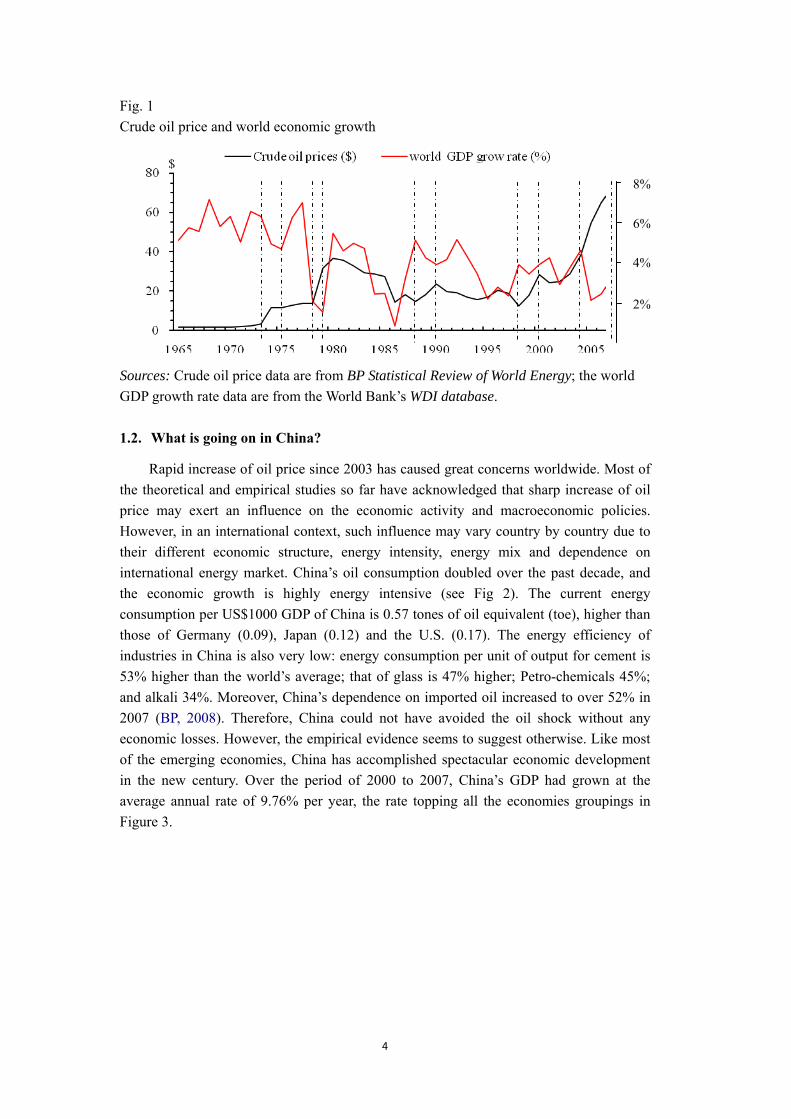
Fig. 1 Crude oil price and world economic growth

8%

6%

4%

2%

Sources: Crude oil price data are from BP Statistical Review of World Energy; the world GDP growth rate data are from the World Bank’s WDI database.

1.2. What is going on in China?

Rapid increase of oil price since 2003 has caused great concerns worldwide. Most of the theoretical and empirical studies so far have acknowledged that sharp increase of oil price may exert an influence on the economic activity and macroeconomic policies. However, in an international context, such influence may vary country by country due to their different economic structure, energy intensity, energy mix and dependence on international energy market. China’s oil consumption doubled over the past decade, and the economic growth is highly energy intensive (see Fig 2). The current energy consumption per US$1000 GDP of China is 0.57 tones of oil equivalent (toe), higher than those of Germany (0.09), Japan (0.12) and the U.S. (0.17). The energy efficiency of industries in China is also very low: energy consumption per unit of output for cement is 53% higher than the world’s average; that of glass is 47% higher; Petro-chemicals 45%; and alkali 34%. Moreover, China’s dependence on imported oil increased to over 52% in 2007 (BP, 2008). Therefore, China could not have avoided the oil shock without any economic losses. However, the empirical evidence seems to suggest otherwise. Like most of the emerging economies, China has accomplished spectacular economic development in the new century. Over the period of 2000 to 2007, China’s GDP had grown at the average annual rate of 9.76% per year, the rate topping all the economies groupings in Figure 3.

  4

Fig. 2 Cross-nation comparison of energy intensity and efficiency

Sources: energy consumption data are from BP Statistical Review of World Energy (2008); GDP data are from the World Bank’s WDI database; and energy efficiency data are from China Energy Statistical Yearbook, 2008. Fig. 3 Average annual GDP growth rates for the past five decades

GD

P growth rate (%

)

Source: The World Bank’s WDI database. Does that suggest that China is less vulnerable to oil shocks than other economies? If

not, is there any possibility for hysteresis in the impact of oil shock? Unfortunately, most of the empirical studies to date have been conducted for the developed nations, and there

  5

has been a lack of empirical evidences for developing countries. In this paper, we attempt to fill this gap by answering how and to what extent oil-price shocks impact China’s economy. The paper emphasizes on the investigation of the transmission mechanisms. Specifically, it will focus on the following two issues: 1) how are the conventional transmission mechanisms modified in the specific context of China; and 2) how do the adverse impact of oil-price shock and its robustness change in the long run in China?

The paper is organized as follows. Section 2 discusses the transmission channels through which oil-price changes affect the macroeconomic variables. Section 3 provides a partial equilibrium analysis of such transmission mechanisms and their effects on the macroeconomic indices of China. The overall impact of oil-price shock is analyzed in Section 4 using a structural vector auto-regressive model. On that base, we disentangle the long-term impact from the overall impact in Section 5. Section 6 presents key findings and conclusions.

2. The Transmission mechanisms

2.1. Transmission channels

From a theoretical perspective, oil-price changes affect the performances of macroeconomic variables through the following six transmission channels (Brown and Yucel, 2002):

• Supply-side shock effect: focusing on the direct impact on output due to the change in marginal producing costs caused by oil-price shock;

• Wealth transfer effect: emphasizing on the different marginal consumption rate of petrodollar and that of ordinary trade surplus;

• Inflation effect: analyzing relationship between domestic inflation and oil prices; • Real balance effect: investigating the change in money demand and monetary

policy; • Sector adjustment effect: estimating the adjustment cost of industrial structure,

which is mainly used to explain the asymmetry in oil-price shock impact; • Unexpected effect: focusing on the uncertainty about oil price and its impact. These channels have been proved to be valid in industrialized countries. However,

whether they still hold in China is an open question. Fig. 4 holds the main idea. Crude oil is one of the most fundamental and crucial raw materials for industrial

production, and the change in its price can affect the output directly. As Arrow ① in Figure 4 indicates, oil-price shocks can increase the marginal cost of production in many industries, and thus reduce the production. This is referred to as the supply-side shock effect. The reduction of output due to the cut of capacity utilization can recover quickly within the range of capacity. However, oil-price shocks also have long-term effect on output which is carried out through Price/Monetary Transmission Mechanism (Arrow ③).

Cost shocks in the upper stream industry can be transmitted from producers and sectors to end-users. A well developed industrial chain can transmit inflationary shock from upper stream to down stream, leaving the producers’ profit rate slightly affected.

  6

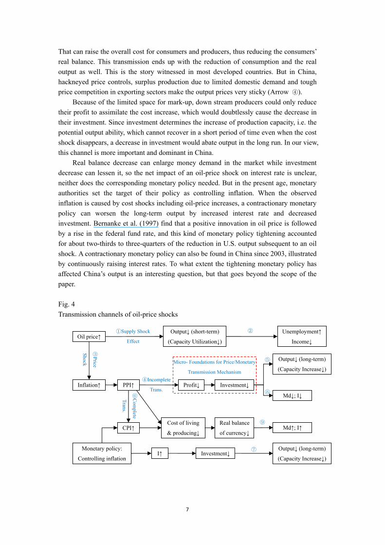
That can raise the overall cost for consumers and producers, thus reducing the consumers’ real balance. This transmission ends up with the reduction of consumption and the real output as well. This is the story witnessed in most developed countries. But in China, hackneyed price controls, surplus production due to limited domestic demand and tough price competition in exporting sectors make the output prices very sticky (Arrow ④).

Because of the limited space for mark-up, down stream producers could only reduce their profit to assimilate the cost increase, which would doubtlessly cause the decrease in their investment. Since investment determines the increase of production capacity, i.e. the potential output ability, which cannot recover in a short period of time even when the cost shock disappears, a decrease in investment would abate output in the long run. In our view, this channel is more important and dominant in China.

Real balance decrease can enlarge money demand in the market while investment decrease can lessen it, so the net impact of an oil-price shock on interest rate is unclear, neither does the corresponding monetary policy needed. But in the present age, monetary authorities set the target of their policy as controlling inflation. When the observed inflation is caused by cost shocks including oil-price increases, a contractionary monetary policy can worsen the long-term output by increased interest rate and decreased investment. Bernanke et al. (1997) find that a positive innovation in oil price is followed by a rise in the federal fund rate, and this kind of monetary policy tightening accounted for about two-thirds to three-quarters of the reduction in U.S. output subsequent to an oil shock. A contractionary monetary policy can also be found in China since 2003, illustrated by continuously raising interest rates. To what extent the tightening monetary policy has affected China’s output is an interesting question, but that goes beyond the scope of the paper.

Fig. 4 Transmission channels of oil-price shocks

⑥Com

plete

Trans.

Micro- Foundations for Price/Monetary

Transmission Mechanism ④Incomplete

Trans.

③Price

Shock

②

⑤

①Supply Shock

Effect Oil price↑ 

Output↓ (short-term)

(Capacity Utilization↓) 

Unemployment↑

Income↓ 

Inflation↑  PPI↑ 

CPI↑ 

Profit↓  Investment↓ 

Output↓ (long-term)

(Capacity Increase↓) 

Md↓; I↓ 

Cost of living

& producing↓ 

Real balance

of currency↓ Md↑; I↑ 

Monetary policy:

Controlling inflation I↑  Investment↓ 

⑧ 

⑨ 

⑦ (Capacity Increase↓) 

Output↓ (long-term)

  7

3. Partial equilibrium analysis of the transmission mechanisms

3.1. Data

In order to test the validity of transmission mechanisms, we employ some macroeconomic variables of China, denoted as follows:

• Real Oil-Price (RP) is the adjusted WTI spot crude price in 1995 Chinese Yuan. Aside from RP, we introduce Positive/Negative Difference of Oil-Price (PDP/NDP) and Net Oil-Price Increase (NPI), which were put forward by Hamilton (1985), to capture the asymmetry in the impact of oil-price shock on economy;

• Consumer/Producer Price Index (CPI/PPI) are in chain-indices; • Real Rate of Return for Industrial Companies (RRT) is the ratio of profit and

capital occupation of product, minus PPI; • Real Interest Rate (RI) is one year loan rate, minus CPI; • Real Investment toward Industry (INV) is in constant price (1995 Chinese Yuan); • Real Industrial Added Value (IAV) is employed to indicate aggregate output, also

in constant price (1995 Chinese Yuan). The sample period is from February 1998 to August 2008, including 127 original

observations. The oil prices data are taken from the U.S. Energy Information Administration (http://tonto.eia.doe.gov); the macro-economic variables of China are derived from the Wind Financial Database named WindDB (http://www.wind.com.cn/en/product/windDB.htm). Census X-12 approach is utilized to eliminate seasonal fluctuations from INV, IAV and RRT. There are no evidences for seasonal patterns in CPI, PPI and RP series (see Table 1).

The census X-12 approach is developed by the U.S. Census Bureau in the late 1990s, for decomposition/adjustment of seasonal time series. It is adapted from the Bureau’s well known X-11 procedure (Shiskin, Young and Musgrave, 1967).1 The core algorithm of Census X-12 approach is based on an Auto-Rregressive Integrated Moving Average (ARIMA) model. The multiplicative form of decomposition was used in this analysis:

tttt ISTCY ⋅⋅=

where Yt is the original series, TCt is the trend cycle, St is the seasonal factors, and It stands for irregular component. There are three more forms of decompositions:

• Additive: ; tttt ISTCY ++=

• Pseudo-additive: ; )1( −+= tttt ISTCY

• Log-additive: . tttt ISTCY lnlnlnln ++=

                                                              1 See Findley et al. (1998) and Ladiray and Quenneville (2001) for more detailed discussion on Census X-12 seasonal adjustment approach, and the U.S. Census Bureau’s website (www.census.gov/ srd/www/x12a) for up-to-date documentation of the X-12-ARIMA program and the program itself. 

  8

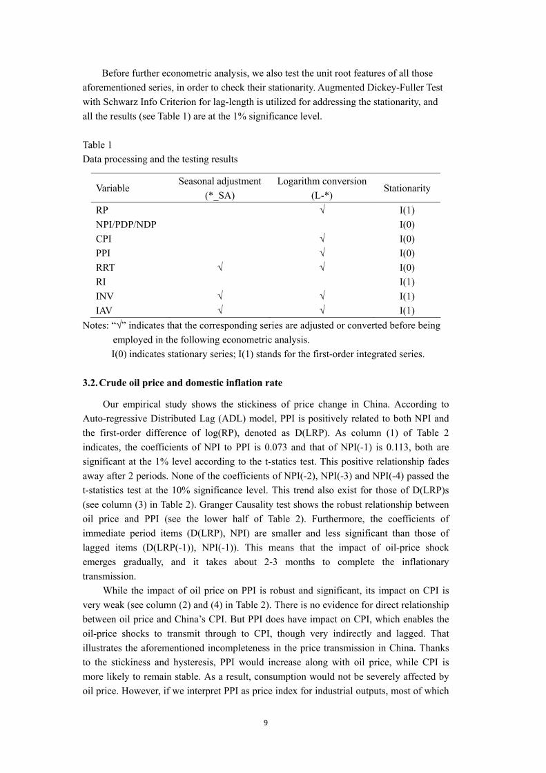
Before further econometric analysis, we also test the unit root features of all those aforementioned series, in order to check their stationarity. Augmented Dickey-Fuller Test with Schwarz Info Criterion for lag-length is utilized for addressing the stationarity, and all the results (see Table 1) are at the 1% significance level. Table 1 Data processing and the testing results

Variable Seasonal adjustment

(*_SA) Logarithm conversion

(L-*) Stationarity

RP √ I(1) NPI/PDP/NDP I(0) CPI √ I(0) PPI √ I(0) RRT √ √ I(0) RI I(1) INV √ √ I(1) IAV √ √ I(1)

Notes: “√” indicates that the corresponding series are adjusted or converted before being employed in the following econometric analysis. I(0) indicates stationary series; I(1) stands for the first-order integrated series.

3.2. Crude oil price and domestic inflation rate

Our empirical study shows the stickiness of price change in China. According to Auto-regressive Distributed Lag (ADL) model, PPI is positively related to both NPI and the first-order difference of log(RP), denoted as D(LRP). As column (1) of Table 2 indicates, the coefficients of NPI to PPI is 0.073 and that of NPI(-1) is 0.113, both are significant at the 1% level according to the t-statics test. This positive relationship fades away after 2 periods. None of the coefficients of NPI(-2), NPI(-3) and NPI(-4) passed the t-statistics test at the 10% significance level. This trend also exist for those of D(LRP)s (see column (3) in Table 2). Granger Causality test shows the robust relationship between oil price and PPI (see the lower half of Table 2). Furthermore, the coefficients of immediate period items (D(LRP), NPI) are smaller and less significant than those of lagged items (D(LRP(-1)), NPI(-1)). This means that the impact of oil-price shock emerges gradually, and it takes about 2-3 months to complete the inflationary transmission.

While the impact of oil price on PPI is robust and significant, its impact on CPI is very weak (see column (2) and (4) in Table 2). There is no evidence for direct relationship between oil price and China’s CPI. But PPI does have impact on CPI, which enables the oil-price shocks to transmit through to CPI, though very indirectly and lagged. That illustrates the aforementioned incompleteness in the price transmission in China. Thanks to the stickiness and hysteresis, PPI would increase along with oil price, while CPI is more likely to remain stable. As a result, consumption would not be severely affected by oil price. However, if we interpret PPI as price index for industrial outputs, most of which

  9

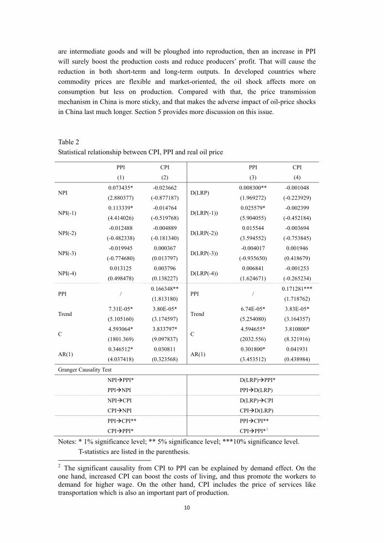
are intermediate goods and will be ploughed into reproduction, then an increase in PPI will surely boost the production costs and reduce producers’ profit. That will cause the reduction in both short-term and long-term outputs. In developed countries where commodity prices are flexible and market-oriented, the oil shock affects more on consumption but less on production. Compared with that, the price transmission mechanism in China is more sticky, and that makes the adverse impact of oil-price shocks in China last much longer. Section 5 provides more discussion on this issue. Table 2 Statistical relationship between CPI, PPI and real oil price

PPI

(1)

CPI

(2)

PPI

(3)

CPI

(4)

NPI 0.073435*

(2.880377)

-0.023662

(-0.877187) D(LRP)

0.008300**

(1.969272)

-0.001048

(-0.223929)

NPI(-1) 0.113339*

(4.414026)

-0.014764

(-0.519768) D(LRP(-1))

0.025579*

(5.904055)

-0.002399

(-0.452184)

NPI(-2) -0.012488

(-0.482338)

-0.004889

(-0.181340) D(LRP(-2))

0.015544

(3.594552)

-0.003694

(-0.753845)

NPI(-3) -0.019945

(-0.774680)

0.000367

(0.013797) D(LRP(-3))

-0.004017

(-0.935650)

0.001946

(0.418679)

NPI(-4) 0.013125

(0.498478)

0.003796

(0.138227) D(LRP(-4))

0.006841

(1.624671)

-0.001253

(-0.265234)

PPI / 0.166348**

(1.813180) PPI /

0.171281***

(1.718762)

Trend 7.31E-05*

(5.105160)

3.80E-05*

(3.174597) Trend

6.74E-05*

(5.254080)

3.83E-05*

(3.164357)

C 4.593064*

(1801.369)

3.833797*

(9.097837) C

4.594655*

(2032.556)

3.810800*

(8.321916)

AR(1) 0.346512*

(4.037418)

0.030811

(0.323568) AR(1)

0.301800*

(3.453512)

0.041931

(0.438984)

Granger Causality Test

NPI PPI* D(LRP) PPI*

PPI NPI PPI D(LRP)

NPI CPI D(LRP) CPI

CPI NPI CPI D(LRP)

PPI CPI** PPI CPI**

CPI PPI* CPI PPI*2

Notes: * 1% significance level; ** 5% significance level; ***10% significance level. T-statistics are listed in the parenthesis.

                                                              2 The significant causality from CPI to PPI can be explained by demand effect. On the one hand, increased CPI can boost the costs of living, and thus promote the workers to demand for higher wage. On the other hand, CPI includes the price of services like transportation which is also an important part of production.  

  10

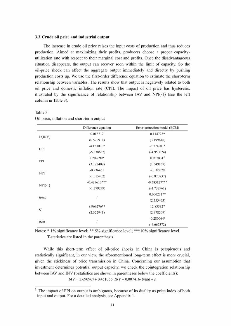
3.3. Crude oil price and industrial output

The increase in crude oil price raises the input costs of production and thus reduces production. Aimed at maximizing their profits, producers choose a proper capacity- utilization rate with respect to their marginal cost and profits. Once the disadvantageous situation disappears, the output can recover soon within the limit of capacity. So the oil-price shock can affect the aggregate output immediately and directly by pushing production costs up. We use the first-order difference equation to estimate the short-term relationship between variables. The results show that output is negatively related to both oil price and domestic inflation rate (CPI). The impact of oil price has hysteresis, illustrated by the significance of relationship between IAV and NPI(-1) (see the left column in Table 3).

Table 3 Oil price, inflation and short-term output

Difference equation Error-correction model (ECM)

D(INV) 0.018717

(0.570914)

0.114723*

(3.199646)

CPI -4.153096*

(-5.338682)

-3.774201*

(-4.950024)

PPI 2.209699*

(3.122402)

0.9828313

(1.349837)

NPI -0.236461

(-1.015402)

-0.185079

(-0.870837)

NPI(-1) -0.427610***

(-1.779239)

-0.383127***

(-1.732961)

trend / 0.000231**

(2.353463)

C 8.969276**

(2.322941)

12.83332*

(2.978209)

ecm / -0.280064*

(-4.667372)

Notes: * 1% significance level; ** 5% significance level; ***10% significance level. T-statistics are listed in the parenthesis.

While this short-term effect of oil-price shocks in China is perspicuous and

statistically significant, in our view, the aforementioned long-term effect is more crucial, given the stickiness of price transmission in China. Concerning our assumption that investment determines potential output capacity, we check the cointegration relationship between IAV and INV (t-statistics are shown in parentheses below the coefficients):

ε+⋅+⋅+= trendINVIAV 007416.0451055.0690967.3                                                               3 The impact of PPI on output is ambiguous, because of its duality as price index of both

input and output. For a detailed analysis, see Appendix 1. 

  11

(27.91022) (13.13232) (10.93728)

The stationarity of the residual series is checked using the ADF,4 PP and KPSS approaches, all indicating I(0) at the 1% significance level. That indicates the existence of cointegration relationship between investment and output. Taking the long-term relationship into account, we can establish an Error-Correction Model (ECM), and the results are more legible (listed on the right column in Table 3).

The cointegration relationship reinforces the argument that investment determines long term output. To separate the long-term effect from the overall effect of an oil price shock, a rigorous analysis is carried out using a structural vector auto-regressive model in section 4. But before that, we first investigate the determinants of investment, in both the short term and long term.

Aside from economic aggregates, interest rate and profit rate also determine investment by changing the costs and benefits of investment. Since profit rate (RRT) is trend stationary, we test the cointegration relationship among INV, IAV and RI (t-statistics are shown in parentheses below the coefficients):

ε+⋅−⋅−⋅+−= trendRIIAVINV 002206.0007105.0309048.1186414.3 (-5.997389) (13.10814) (-1.053999) (-1.272779)

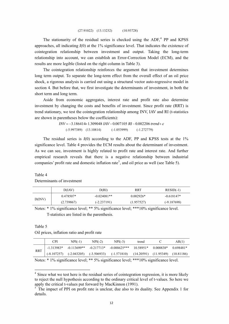
The residual series is I(0) according to the ADF, PP and KPSS tests at the 1% significance level. Table 4 provides the ECM results about the determinant of investment. As we can see, investment is highly related to profit rate and interest rate. And further empirical research reveals that there is a negative relationship between industrial companies’ profit rate and domestic inflation rate5, and oil price as well (see Table 5).

Table 4 Determinants of investment

D(IAV) D(RI) RRT RESID(-1)

D(INV) 0.478507*

(2.739867)

-0.024081**

(-2.237191)

0.002926*

(1.957527)

-0.618147*

(-9.187698)

Notes: * 1% significance level; ** 5% significance level; ***10% significance level. T-statistics are listed in the parenthesis.

Table 5 Oil prices, inflation ratio and profit rate

CPI NPI(-1) NPI(-2) NPI(-3) trend C AR(1)

RRT -1.313983*

(-8.107257)

-0.113699**

(-2.043205)

-0.217713*

(-3.506933)

-0.088625***

(-1.571810)

10.58951*

(14.20591)

0.000838*

(11.95349)

0.698481*

(10.81186)

Notes: * 1% significance level; ** 5% significance level; ***10% significance level.

                                                              4 Since what we test here is the residual series of cointegration regression, it is more likely to reject the null hypothesis according to the ordinary critical level of t-values. So here we apply the critical t-values put forward by MacKinnon (1991). 5 The impact of PPI on profit rate is unclear, due also to its duality. See Appendix 1 for details.  

  12

t-statistics are listed in the parenthesis. PPI and NPI are not included in the equation, because their coefficients fail to pass the significance test.

3.4. Brief summary of transmission mechanisms in China

An increase in crude oil price can affect the short term output of an economy by directly raising the marginal cost for industrial production and change the profit-maximizing capacity-utilizing rate. Once the disadvantageous situation disappears, the production can recover soon within the limit of capacity. But there are some effects of oil-price shock that cannot recover quickly. Change in production cost would affect profit rate of producers, which is the primary profit of investment. Given the fact that investment determines output in the long run, the long-term effect of oil shock is more important than the short-term effect.

Price controls, surplus production caused by limited domestic demand, excessive price competition in international trade make the CPI very sticky in China. The stickiness and hysteresis of the inflationary shock transmission cut the profit rate of producers which cause the reduction in both short-term and long-term outputs. Compared with developed countries, the baffled price transmission mechanism in China makes the adverse impact of inflationary shocks more serious and permanent.

4. General equilibrium analysis by the SVAR model

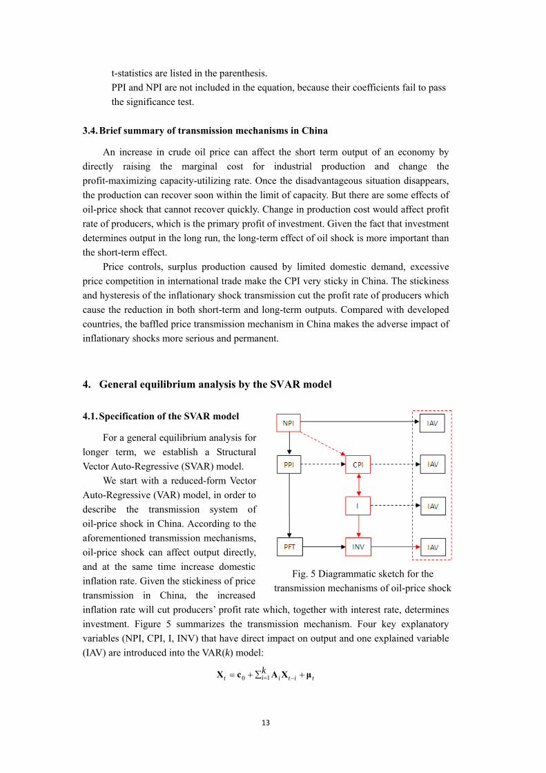
4.1. Specification of the SVAR model

For a general equilibrium analysis for longer term, we establish a Structural Vector Auto-Regressive (SVAR) model.

We start with a reduced-form Vector Auto-Regressive (VAR) model, in order to describe the transmission system of oil-price shock in China. According to the aforementioned transmission mechanisms, oil-price shock can affect output directly, and at the same time increase domestic inflation rate. Given the stickiness of price transmission in China, the increased inflation rate will cut producers’ profit rate which, together with interest rate, determines investment. Figure 5 summarizes the transmission mechanism. Four key explanatory variables (NPI, CPI, I, INV) that have direct impact on output and one explained variable (IAV) are introduced into the VAR(k) model:

Fig. 5 Diagrammatic sketch for the transmission mechanisms of oil-price shock

ti ititk μXAcX +∑+= = −10

  13

Xt is the vector of the five endogenous variables, { }NPICPIIINVIAV ,,,,= tttttt′X ;

μt is the vector of residuals, which are used to estimate the structural restrictions; c0 and Ai are vector/matrix for constants and coefficients which need to be estimated; k is the number of lagged terms. VAR estimations are very sensitive to lag structure

of variables. A sufficient lag length does help to reflect the long-term impact of variables on others, but adding lag length will cause collinearity problems, let alone lessen the degrees of freedom (DOF). For any k ≥11, the model will become divergent with at least one Auto-Regressive Roots greater than unit. According to sequential modified Likelihood Ratio test static (LR), lag order of 1-3 is the best for our model (k=3)6.

Since only the lagged terms are listed on the right-hand side of VAR equation, a reduced-form VAR model is unable to analyze the contemporanous relationship among variables, which causes cross-correlation among residual series, i.e. the covariance matrix

of residuals . Although it does not affect the unbiasness and efficiency of

the estimation, the contemporoneous relationship may affect the impulse response ramarkably. So we introduce the contemporaneous coefficients matrix B into the VAR model as structural restrictions:

IμμΣ ≠′= )( ttE

∑ ++= = −ki titit 100 εXBcXB

B0 is a k*k non-identity matrix (note that if B0 is an identity matrix, then the SVAR

model would retrogress into a reduced-form VAR model), εt is a k*1 vector of residuals

which satisfies the condition that , that is, the residuals are uncorrelated white

noise series. Rewrite a reduced-form VAR in lag operator:

Iεε =′ )( ttE

ttL μXA =)(

Assume that there is a invertible matrix Bk*k:

tttL εBμXBA ==)(

Since , and ∑ is already identified by μt, we have

actually applied k(k+1)/2 restrictions, and we need another k(k−1)/2 restrictions to identify the structural restriction matrix B.

IBBΣBμBμεε =′=′=′ )()( tttt EE

For the extra 10 restrictions, we turn to the economic theory. It is reasonable to                                                               6 The unit root test indicated that IAV, INV and I employed in the VAR model are I(1) series, but the nonstationary problem can be absorbed by introducing more lagged terms, so the theoretical stationarity assumption is not very strict. The 3 stage lag length is sufficient to absorb the nonstationarity, for the residual series of 5 VAR equations are all stationary. We also utilize the VEC module to estimate the mutual relationship among variables, and the result is very similar to the VAR estimation. See Appendix 2 for detailed analysis. 

  14

assume that oil price is exogenous (only) at the contemporaneous period (i.e. for t=0, b51, b52, b53, b54=0), and it can affect all the other four endogenous variables:

NPIbNPI ⋅= 55 .

The second restriction is that CPI is only determined by oil price and CPI itself, which means a change in interest rate, investment and output can only affect CPI in the subsequent periods (b41, b42, b43=0).

NPIbCPIbCPI ⋅+⋅= 4544 .

The third restriction specifies that interest rate does not respond to either IAV or INV, because of the time lag (b31, b32=0).

NPIbCPIbIbI ⋅+⋅+⋅= 353433 .

In the last restriction, we assume that output change does not affect investment immediately, but the investment change affect output instantly (b21=0).

NPIbCPIbIbINVbINV ⋅++⋅+⋅= 25242322 ;

NPIbCPIbIbINVbIAVbIAV ⋅++⋅+⋅+⋅= 1514131211 .

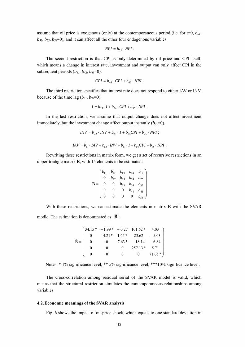
Rewriting these restrictions in matrix form, we get a set of recursive restrictions in an upper-triabgle matrix B, with 15 elements to be estimated:

⎟⎟⎟⎟⎟

⎠

⎞

⎜⎜⎜⎜⎜

⎝

⎛

=

55

4544

353433

25242322

1514131211

0000000

000

bbbbbbbbbbbbbbb

B

With these restrictions, we can estimate the elements in matrix B with the SVAR

modle. The estimation is denominated as : B̂

⎟⎟⎟⎟⎟

⎠

⎞

⎜⎜⎜⎜⎜

⎝

⎛

−−−

−−

=

*65.71000071.5*13.25700084.614.18*63.70003.562.23*65.1*21.140

03.4*62.10127.0*99.1*34.15

B̂

Notes: * 1% significance level; ** 5% significance level; ***10% significance level. The cross-correlation among residual serial of the SVAR model is valid, which

means that the structural restriction simulates the contemporaneous relationships among variables. 4.2. Economic meanings of the SVAR analysis

Fig. 6 shows the impact of oil-price shock, which equals to one standard deviation in

  15

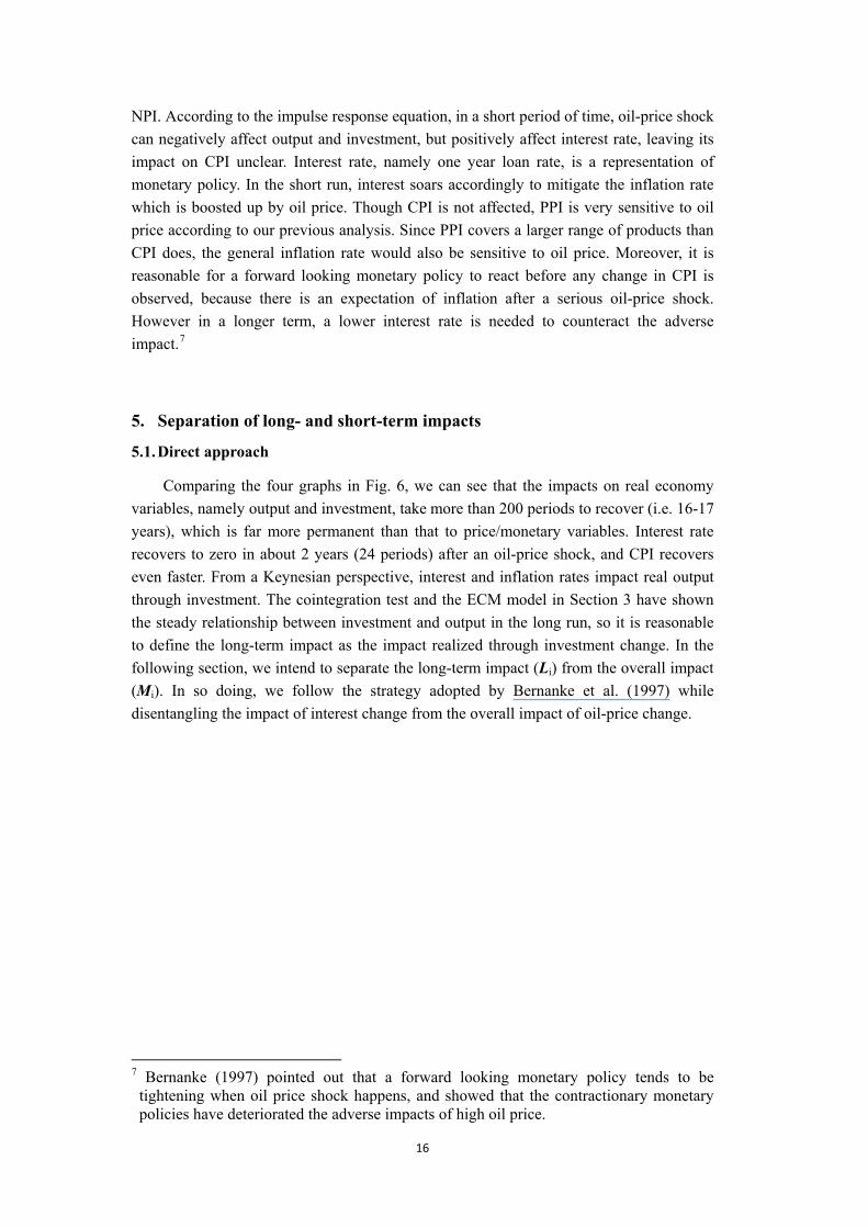
NPI. According to the impulse response equation, in a short period of time, oil-price shock can negatively affect output and investment, but positively affect interest rate, leaving its impact on CPI unclear. Interest rate, namely one year loan rate, is a representation of monetary policy. In the short run, interest soars accordingly to mitigate the inflation rate which is boosted up by oil price. Though CPI is not affected, PPI is very sensitive to oil price according to our previous analysis. Since PPI covers a larger range of products than CPI does, the general inflation rate would also be sensitive to oil price. Moreover, it is reasonable for a forward looking monetary policy to react before any change in CPI is observed, because there is an expectation of inflation after a serious oil-price shock. However in a longer term, a lower interest rate is needed to counteract the adverse impact.7

5. Separation of long- and short-term impacts

5.1. Direct approach

Comparing the four graphs in Fig. 6, we can see that the impacts on real economy variables, namely output and investment, take more than 200 periods to recover (i.e. 16-17 years), which is far more permanent than that to price/monetary variables. Interest rate recovers to zero in about 2 years (24 periods) after an oil-price shock, and CPI recovers even faster. From a Keynesian perspective, interest and inflation rates impact real output through investment. The cointegration test and the ECM model in Section 3 have shown the steady relationship between investment and output in the long run, so it is reasonable to define the long-term impact as the impact realized through investment change. In the following section, we intend to separate the long-term impact (Li) from the overall impact (Mi). In so doing, we follow the strategy adopted by Bernanke et al. (1997) while disentangling the impact of interest change from the overall impact of oil-price change.

                                                              7 Bernanke (1997) pointed out that a forward looking monetary policy tends to be tightening when oil price shock happens, and showed that the contractionary monetary policies have deteriorated the adverse impacts of high oil price. 

  16

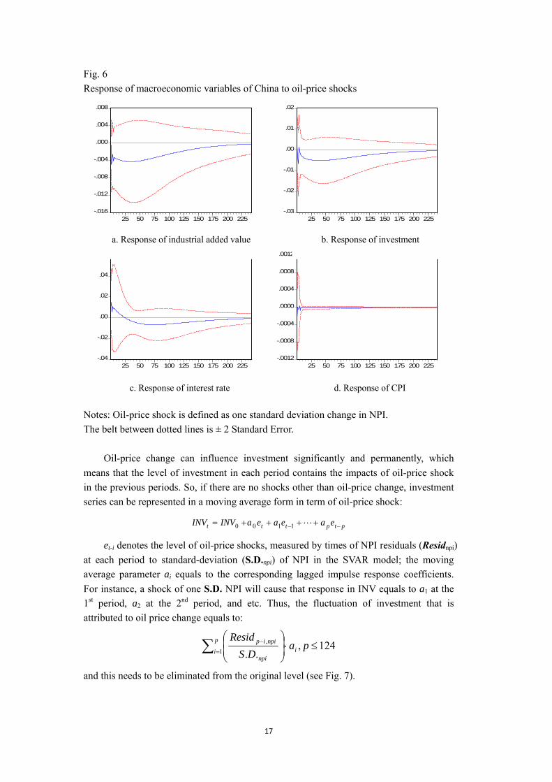
Fig. 6 Response of macroeconomic variables of China to oil-price shocks

-.016

-.012

-.008

-.004

.000

.004

.008

25 50 75 100 125 150 175 200 225-.03

-.02

-.01

.00

.01

.02

25 50 75 100 125 150 175 200 225

-.04

-.02

.00

.02

.04

.06

25 50 75 100 125 150 175 200 225

Response of I to Shock5

-.0012

-.0008

-.0004

.0000

.0004

.0008

.0012

25 50 75 100 125 150 175 200 225

Response of LOG(CPI2_SA) to Shock5

b. Response of investment a. Response of industrial added value  

c. Response of interest rate d. Response of CPI Notes: Oil-price shock is defined as one standard deviation change in NPI. The belt between dotted lines is ± 2 Standard Error.

Oil-price change can influence investment significantly and permanently, which means that the level of investment in each period contains the impacts of oil-price shock in the previous periods. So, if there are no shocks other than oil-price change, investment series can be represented in a moving average form in term of oil-price shock:

ptpttt eaeaeaINVINV −− ++++= L1100

et-i denotes the level of oil-price shocks, measured by times of NPI residuals (Residnpi) at each period to standard-deviation (S.D.npi) of NPI in the SVAR model; the moving average parameter ai equals to the corresponding lagged impulse response coefficients. For instance, a shock of one S.D. NPI will cause that response in INV equals to a1 at the 1st period, a2 at the 2nd period, and etc. Thus, the fluctuation of investment that is attributed to oil price change equals to:

124,..1

, ≤⋅⎟⎟⎠

⎞⎜⎜⎝

⎛∑ =

− paDS

Residi

p

inpi

npiip

and this needs to be eliminated from the original level (see Fig. 7).

  17

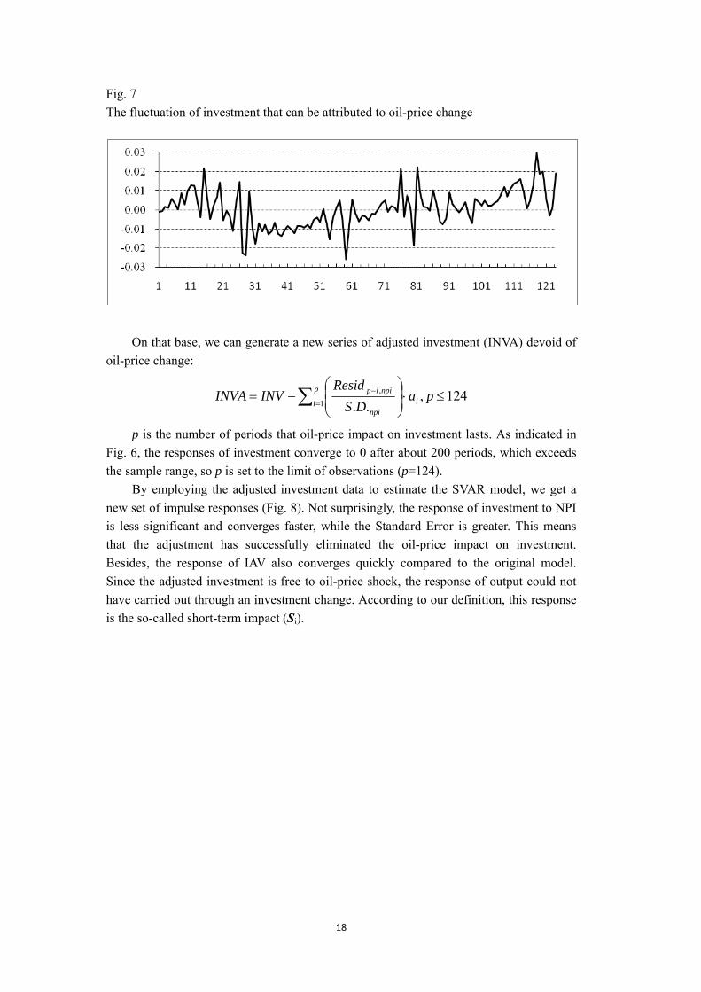
Fig. 7 The fluctuation of investment that can be attributed to oil-price change

On that base, we can generate a new series of adjusted investment (INVA) devoid of

oil-price change:

124,..1

, ≤⋅⎟⎟⎠

⎞⎜⎜⎝

⎛−= ∑ =

− paDS

ResidINVINVA i

p

inpi

npiip

p is the number of periods that oil-price impact on investment lasts. As indicated in Fig. 6, the responses of investment converge to 0 after about 200 periods, which exceeds the sample range, so p is set to the limit of observations (p=124).

By employing the adjusted investment data to estimate the SVAR model, we get a new set of impulse responses (Fig. 8). Not surprisingly, the response of investment to NPI is less significant and converges faster, while the Standard Error is greater. This means that the adjustment has successfully eliminated the oil-price impact on investment. Besides, the response of IAV also converges quickly compared to the original model. Since the adjusted investment is free to oil-price shock, the response of output could not have carried out through an investment change. According to our definition, this response is the so-called short-term impact (Si).

  18

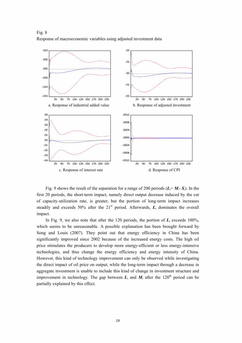
Fig. 8 Response of macroeconomic variables using adjusted investment data

-.015

-.010

-.005

.000

.005

.010

25 50 75 100 125 150 175 200 225-.02

-.01

.00

.01

.02

25 50 75 100 125 150 175 200 225

-.04

-.03

-.02

-.01

.00

.01

.02

.03

.04

.05

25 50 75 100 125 150 175 200 225

Response of I to Shock5

-.0012

-.0008

-.0004

.0000

.0004

.0008

.0012

25 50 75 100 125 150 175 200 225

Response of LOG(CPI2_SA) to Shock5

a. Response of industrial added value b. Response of adjusted investment  

c. Response of interest rate d. Response of CPI

Fig. 9 shows the result of the separation for a range of 200 periods (Li= Mi- Si). In the

first 20 periods, the short-term impact, namely direct output decrease induced by the cut of capacity-utilization rate, is greater, but the portion of long-term impact increases steadily and exceeds 50% after the 21st period. Afterwards, Li dominates the overall impact.

In Fig. 9, we also note that after the 120 periods, the portion of Li exceeds 100%, which seems to be unreasonable. A possible explanation has been brought forward by Song and Louis (2007). They point out that energy efficiency in China has been significantly improved since 2002 because of the increased energy costs. The high oil price stimulates the producers to develop more energy-efficient or less energy-intensive technologies, and thus change the energy efficiency and energy intensity of China. However, this kind of technology improvement can only be observed while investigating the direct impact of oil price on output, while the long-term impact through a decrease in aggregate investment is unable to include this kind of change in investment structure and improvement in technology. The gap between Li and Mi after the 120th period can be partially explained by this effect.

  19

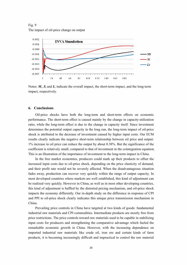
Fig. 9 The impact of oil-price change on output

Notes: Mi, Si and Li indicate the overall impact, the short-term impact, and the long-term impact, respectively.

6. Conclusions

Oil-price shocks have both the long-term and short-term effects on economic performance. The short-term effect is caused mainly by the change in capacity-utilization ratio, while the long-term effect is due to the change in capacity itself. Since investment determines the potential output capacity in the long run, the long-term impact of oil-price shock is attributed to the decrease of investment caused by higher input costs. Our ECM results clearly indicate the negative short-term relationship between oil price and output: 1% increase in oil price can reduce the output by about 0.38%. But the significance of the coefficient is relatively small, compared to that of investment in the cointegration equation. This is an illustration of the importance of investment to the long-term impact in China.

In the free market economies, producers could mark up their products to offset the increased input costs due to oil-price shock, depending on the price elasticity of demand, and their profit rate would not be severely affected. When the disadvantageous situation fades away, production can recover very quickly within the range of output capacity. In most developed countries where markets are well established, this kind of adjustment can be realized very quickly. However in China, as well as in most other developing countries, this kind of adjustment is baffled by the distorted pricing mechanism, and oil-price shock impacts the economy differently. Our in-depth study on the difference in response of CPI and PPI to oil-price shock clearly indicates this unique price transmission mechanism in China.

Prevailing price controls in China have targeted at two kinds of goods: fundamental industrial raw materials and CPI commodities. Intermediate products are mostly free from price restrictions. The price controls toward raw materials used to be capable in stabilizing input costs for producers and strengthening the comparative advantage which fueled the remarkable economic growth in China. However, with the increasing dependence on imported industrial raw materials like crude oil, iron ore and certain kinds of farm products, it is becoming increasingly difficult and impractical to control the raw material

  20

prices in China. Meanwhile, the oil pricing system on domestic market went through two revolutions from the late 1990s to the early 2000s: the first was in 1998, which pegged the prices of crude and petrochemical products to Singapore market; the second was in 2001, two more markets, Rotterdam and New York were brought into equation. We can see that the domestic oil prices are becoming increasingly related to the world market, and price controls are losing their effectiveness gradually. According to our partial equilibrium analysis, PPI is positively related to oil price: 100% increase in oil price can cause 7.34% increase in PPI in the same month, and 11.33% in the following month. On the other hand, CPI commodities are still under strict restriction. Our empirical research finds no evidences for a direct relationship between oil price and CPI. This structure of price control keeps the price of final output under restriction, and at the same time leaves input costs floating. For consumers, the baffled price transmission mechanism stabilizes commodity prices even when oil-price shock happens. This can somewhat mitigate the short-term effect. For producers, their aggregate profit rate is more sensitive to oil-price shocks because of limited space for them to mark up their products. This would doubtlessly cause the decrease in investment, and thus amplify the long-term impact.

Appendix 1 provides a detailed analysis of the impact of CPI and PPI in different sectors. The sectoral analysis shows that profit rates of upper-stream industries (including oil industry, nonferrous metals processing, steel-making & processing, chemical industry and chemical fiber industry) tend to be positively related to PPI but negatively to CPI; down-stream industries (including machinery manufacturing, plastic industry, food processing, medicine & pharmaceutical industry, textile industry and garment industry) tend to respond otherwise. But aggregate profit rate can be lessened by oil-price shock, so does investment (see Tables 4 and 5).

We establish a SVAR model to undertake a general equilibrium analysis of the impact of oil-price shock. According to the impulse response equation, oil-price increase can negatively affect output and investment, but positively affect inflation rate and interest rate. The impact on real economy, represented by real output and real investment, takes more longer to recover, which is far more permanent than that to price/monetary variables (CPI/PPI/I).

On the base of the SVAR model, the effect of oil-price shock is decomposed into the short-term and long-term impacts. Our decomposition results show that the short-term impact, namely output decrease induced by the cut of capacity-utilization rate, is greater in the first 1 or 2 years, but the portion of the long-term impact, defined as the impact realized through an investment change, increases steadily and exceeds 50% at the 20th period. After the 21 periods, the long-term impact dominates, and maintains for quite some time.

To mitigate the long-term impact of oil-price shocks in China, we like to highlight some measures that need to be taken. First, removing some unnecessary price restrictions can improve the market structure and price transmission mechanisms. Price adjustment can cushion cost increases to producers and prevent their profit rates, as well as investment, from sharp decrease. Second, measures expanding domestic and export demands are needed. The expanded demand can offset the cost increase caused by oil-price shock and stimulate output. Third, since investment determines the long-term

  21

effect of oil-price shock, lower interest rate is needed to stimulate investment and counteract the adverse impact. A contractionary monetary policy subsequent to an oil-price shock can worsen the long-term output, being responsible for about two-thirds to three-quarters of the reduction in U.S. output subsequent to an oil shock. In our view, however, this is the area where more rigorous studies in China are needed to draw any further conclusion about the proper monetary policy in China. Last but not least, improving energy efficiency is widely considered as the most effective and lowest cost means of cutting energy use in responding to high energy prices. Strengthening energy-saving efforts via both technology improvements and sectoral adjustments towards a less energy-intensive economic structure and scaling up the use of renewable energies will enable China to sustain its economic growth while preserving the environment. That would be a win-win situation for China and the planet.

  22

Appendix 1

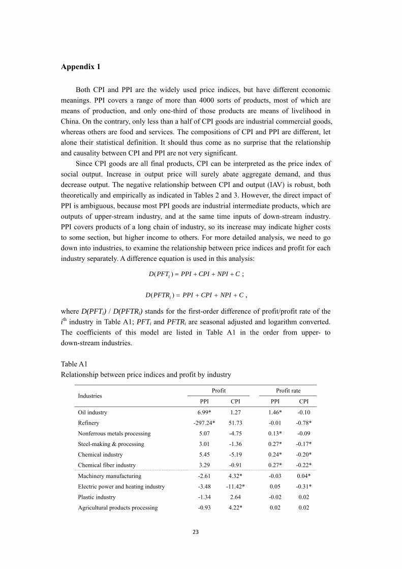
Both CPI and PPI are the widely used price indices, but have different economic meanings. PPI covers a range of more than 4000 sorts of products, most of which are means of production, and only one-third of those products are means of livelihood in China. On the contrary, only less than a half of CPI goods are industrial commercial goods, whereas others are food and services. The compositions of CPI and PPI are different, let alone their statistical definition. It should thus come as no surprise that the relationship and causality between CPI and PPI are not very significant.

Since CPI goods are all final products, CPI can be interpreted as the price index of social output. Increase in output price will surely abate aggregate demand, and thus decrease output. The negative relationship between CPI and output (IAV) is robust, both theoretically and empirically as indicated in Tables 2 and 3. However, the direct impact of PPI is ambiguous, because most PPI goods are industrial intermediate products, which are outputs of upper-stream industry, and at the same time inputs of down-stream industry. PPI covers products of a long chain of industry, so its increase may indicate higher costs to some section, but higher income to others. For more detailed analysis, we need to go down into industries, to examine the relationship between price indices and profit for each industry separately. A difference equation is used in this analysis:

CNPICPIPPIPFTD i +++=)( ;

CNPICPIPPIPFTRD i +++=)( ,

where D(PFTi) / D(PFTRi) stands for the first-order difference of profit/profit rate of the ith industry in Table A1; PFTi and PFTRi are seasonal adjusted and logarithm converted. The coefficients of this model are listed in Table A1 in the order from upper- to down-stream industries.

Table A1 Relationship between price indices and profit by industry

Profit Profit rate Industries

PPI CPI PPI CPI

Oil industry 6.99* 1.27 1.46* -0.10

Refinery -297.24* 51.73 -0.01 -0.78*

Nonferrous metals processing 5.07 -4.75 0.13* -0.09

Steel-making & processing 3.01 -1.36 0.27* -0.17*

Chemical industry 5.45 -5.19 0.24* -0.20*

Chemical fiber industry 3.29 -0.91 0.27* -0.22*

Machinery manufacturing -2.61 4.32* -0.03 0.04*

Electric power and heating industry -3.48 -11.42* 0.05 -0.31*

Plastic industry -1.34 2.64 -0.02 0.02

Agricultural products processing -0.93 4.22* 0.02 0.02

  23

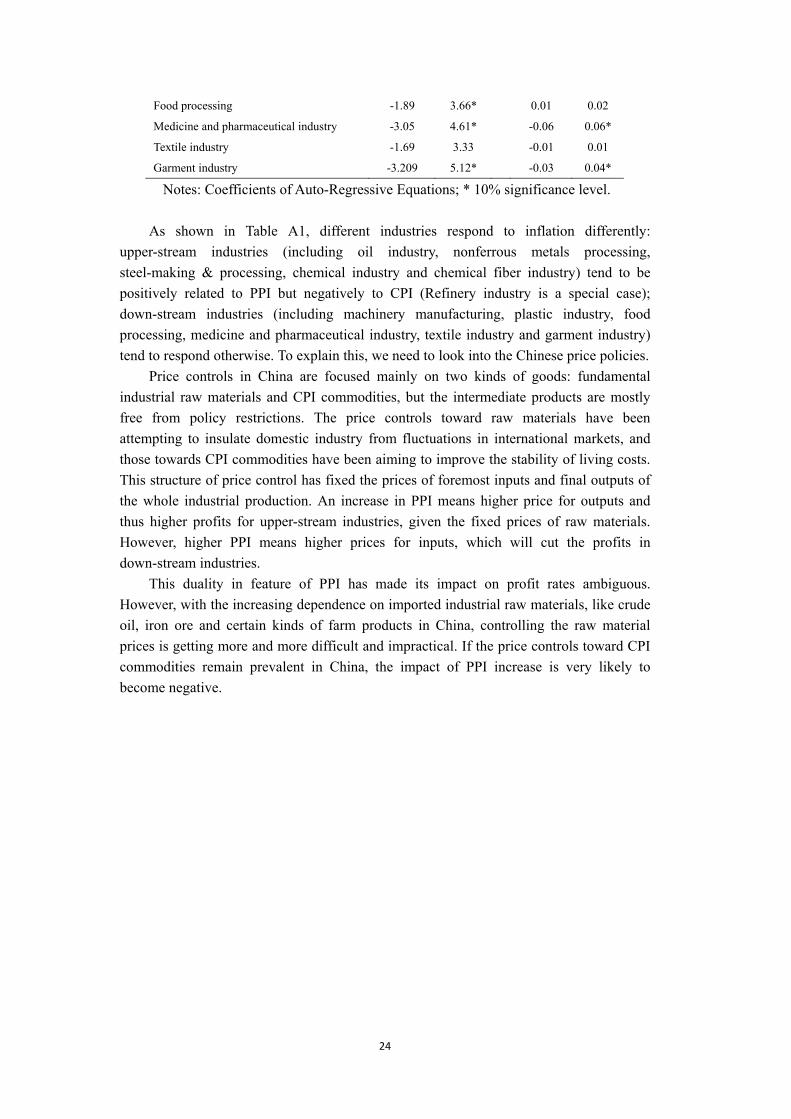
Food processing -1.89 3.66* 0.01 0.02

Medicine and pharmaceutical industry -3.05 4.61* -0.06 0.06*

Textile industry -1.69 3.33 -0.01 0.01

Garment industry -3.209 5.12* -0.03 0.04*

Notes: Coefficients of Auto-Regressive Equations; * 10% significance level. As shown in Table A1, different industries respond to inflation differently:

upper-stream industries (including oil industry, nonferrous metals processing, steel-making & processing, chemical industry and chemical fiber industry) tend to be positively related to PPI but negatively to CPI (Refinery industry is a special case); down-stream industries (including machinery manufacturing, plastic industry, food processing, medicine and pharmaceutical industry, textile industry and garment industry) tend to respond otherwise. To explain this, we need to look into the Chinese price policies.

Price controls in China are focused mainly on two kinds of goods: fundamental industrial raw materials and CPI commodities, but the intermediate products are mostly free from policy restrictions. The price controls toward raw materials have been attempting to insulate domestic industry from fluctuations in international markets, and those towards CPI commodities have been aiming to improve the stability of living costs. This structure of price control has fixed the prices of foremost inputs and final outputs of the whole industrial production. An increase in PPI means higher price for outputs and thus higher profits for upper-stream industries, given the fixed prices of raw materials. However, higher PPI means higher prices for inputs, which will cut the profits in down-stream industries.

This duality in feature of PPI has made its impact on profit rates ambiguous. However, with the increasing dependence on imported industrial raw materials, like crude oil, iron ore and certain kinds of farm products in China, controlling the raw material prices is getting more and more difficult and impractical. If the price controls toward CPI commodities remain prevalent in China, the impact of PPI increase is very likely to become negative.

  24

Appendix 2

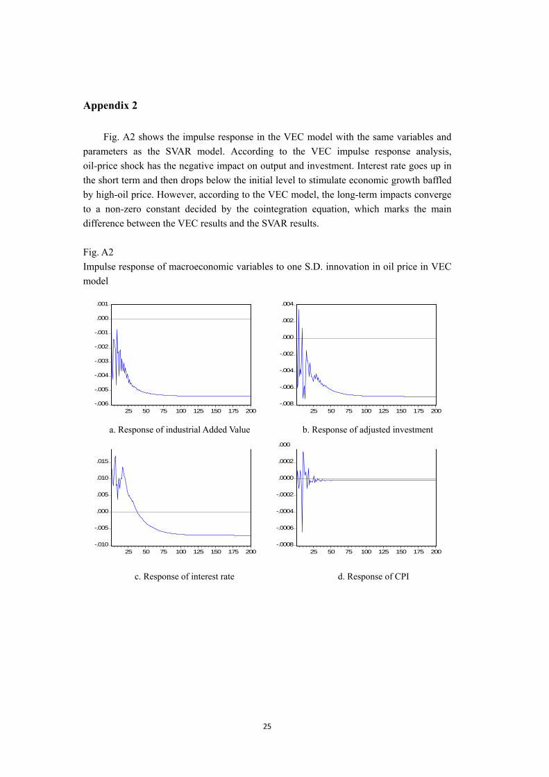
Fig. A2 shows the impulse response in the VEC model with the same variables and parameters as the SVAR model. According to the VEC impulse response analysis, oil-price shock has the negative impact on output and investment. Interest rate goes up in the short term and then drops below the initial level to stimulate economic growth baffled by high-oil price. However, according to the VEC model, the long-term impacts converge to a non-zero constant decided by the cointegration equation, which marks the main difference between the VEC results and the SVAR results. Fig. A2 Impulse response of macroeconomic variables to one S.D. innovation in oil price in VEC model

-.006

-.005

-.004

-.003

-.002

-.001

.000

.001

25 50 75 100 125 150 175 200-.008

-.006

-.004

-.002

.000

.002

.004

25 50 75 100 125 150 175 200

-.010

-.005

.000

.005

.010

.015

.020

25 50 75 100 125 150 175 200

Response of I to NPI

-.0008

-.0006

-.0004

-.0002

.0000

.0002

.0004

25 50 75 100 125 150 175 200

Response of LCPI2 to NPI

a. Response of industrial Added Value  

b. Response of adjusted investment

c. Response of interest rate d. Response of CPI

  25

Reference

Abel, A.B., Bernanke, B.S., 2001. Macroeconomics. Addison-Wesley Longman Inc.

Atkeson, A., Kehoe, P.J., 1999. Models of energy use: putty-putty vs. putty-clay. American Economic Review 89, 1028–1043.

Bacon, R.W., 1991. Rockets and feathers: the asymmetric speed of adjustment of U.K. retail gasoline prices to cost changes. Energy Economics 13, 211–218.

Balke, N.S., Fomby, T.B., 1997. Threshold cointegration. International Economic Review 38, 627–645.

Bernanke, B.S., Gertler, M., Watson, M., 1997. Systematic monetary policy and the effects of oil price shock. Brookings papers on Economic Activity 1, 91-142.

BP (2008), BP Statistical Review of World Energy, British Petroleum (BP), London.

Brown, S.P.A., Yu¨ cel, M.K., 1999. Oil prices and U.S. aggregate economic activity: A question of neutrality. Federal Reserve Bank of Dallas Economic and Financial Review, 16–53.

Brown, S.P.A., Yu¨ cel, M.K., 2002. Energy prices and aggregate economic activity: an interpretative survey. Quarterly Review of Economics and Finance 42, 193–208.

Bruno, M., Sachs, J., 1982. Input price shocks and the slowdown in economic growth: the case of UK manufacturing. Review of Economic Studies 51, 679-705

Burbidge, J., Harrison, A., 1984. Testing for the effects of oil-price rise using vector autoregressions. International Economic Review 25, 459–484.

Byung Rhae Lee, Kiseok Lee, Ronald A. Ratti, 2001. Monetary policy, oil price shocks, and the Japanese economy. Japan and the World Economy 13, 321-349.

Cologni, A.,Manera,M.,2008.Oil prices, inflation and interest rates in a structural cointegrated VAR model for the G-7 countries. Energy Economics 30 (3), 856-888.

Cunado, J., Perez de Gracia, F., 2003. Do oil price shocks matter? Evidence for some European Countries. Energy Economics 25 (2), 137–154.

Dohner, R.S., 1981. Energy prices, economic activity and inflation: survey of issues and results. In: Mork, K.A. (Ed.), Energy Prices, Inflation and Economic Activity. Ballinger, Cambridge, MA.

Findley, D. F., Monsell, B. C., Bell, W. R., Otto, M. C., and Chen, B. C., 1998. New Capabilities and Methods of the X-12-ARIMA Seasonal Adjustment Program. Journal of Business and Economic Statistics 16, 127--176.

Gisser, M., Goodwin, T.H., 1986. Crude oil and the macroeconomy: tests of some popular notions. Journal of Money, Credit and Banking 18, 95–103.

Hamilton, J.D., 1983. Oil and the macroeconomy since World War II. Journal of Political

  26

Economy 91, 228–248.

Hamilton, J.D., 1996. This is what happened to the oil price-macroeconomy relationship. Journal of Monetary Economics 38, 215–220.

Hamilton, J.D., Herrera, A.M., 2004. Oil shocks and aggregate macroeconomic behavior: the role of monetary policy. Journal of Money, Credit, and Banking 36, 265–286.

Hooker, M., 1996. What happened to the oil price-macroeconomy relationship? Journal of Monetary Economics 38, 195–213.

Huang, B.-N., Hwang, M.J., Peng, H.-P., 2005. The asymmetry of the impact of oil price shocks on economic activities: an application of the multivariate threshold model. Energy Economics 27, 455–476.

Kim. S., Kuijs, L., 2007. Raw material prices, wages and profitability in China’s industry — how was profitability maintained when input prices and wages increased so fast?. World Bank China Research Paper No. 8, Washington, DC.

Ladiray, D., Quenneville, B., 2001. Seasonal adjustment with the X-11 method. Springer-Verlag New York.

Lardic,S., Mignon.R. 2006. The impact of oil prices on GDP in European countries: An empirical investigation based on asymmetric cointegration, Energy Policy 34, 3910–3915.

Leduc, S., Sill, K., 2004. A quantitative analysis of oil price shocks, systematic monetary policy and economic downturns. Journal of Monetary Economics 51, 781–808.

Lee, B.R., Lee, K., Ratti, R.A., 2001. Monetary policy, oil price shocks, and the Japanese economy. Japan and the World Economy 13, 321–349.

Lee, K., Ni, S., 2002. On the dynamic effects of oil price shocks: a study using industry level data. Journal of Monetary Economics 49, 823–852.

Lee, K., Ni, S., Ratti, R.A., 1995. Oil shocks and the macroeconomy: the role of price volatility. Energy Journal 16, 39–56.

Lilien, D., 1982. Sectoral shifts and cyclical unemployment. Journal of Political Economy 90, 777–793.

Loungani, P., 1986. Oil price shocks and the dispersion hypothesis. Review of Economics and Statistics 58, 536–539.

Mackinnon, J. G., 1991. Critical values for cointegration tests. In: R.F. Engle and C.W. J. Granger (eds.), Long-run Economic Relationships: Readings in Cointegration. Oxford University Press.

Mork, K.A., 1989. Oil and the macroeconomy when prices go up and down: an extension of Hamilton’s results. Journal of Political Economy 97, 740–744.

Mork, K.A., 1994. Business cycles and the oil market. The Energy Journal 15, 15–38.

  27

  28

Mork, K.A., Olsen, O., Mysen, H.T., 1994. Macroeconomic responses to oil price increases and decreases in seven OECD countries. Energy Journal 15, 19–35.

Mory, J.F., 1993. Oil prices and economic activity: is the relationship symmetric?. The Energy Journal 14, 151–161.

Olsen, O., Mysen, H., 1994. Macroeconomic responses to oil price increases and decreases in seven OECD countries. Energy Journal 15, 19–35.

Pierce, J.L., Enzler, J.J., 1974. The effects of external inflationary shocks. Brookings Papers on Economic Activity 1, 13–61.

Shiskin, J., Young, A. H., and Musgrave, J. C., 1967. The X-11 variant of the Census method II seasonal adjustment program. Technical Paper 15, Bureau of the Census, U.S. Department of Commerce, Washington, DC.