OBTAINING MODE SHAPES THROUGH THE KARHUNEN-L EVE EXPANSION FOR DISTRIBUTED-PARAMETER LINEAR SYSTEMS

OBTAINING MODE SHAPES THROUGH THE

KARHUNEN-LOEVE EXPANSION FOR

DISTRIBUTED-PARAMETER LINEAR SYSTEMS

Claudio Wolter∗ Marcelo A. Trindade†

Rubens Sampaio‡

Dynamics and Vibration Laboratory, Pontifıcia Universidade Catolica do Rio de Janeiro,

rua Marques de Sao Vicente 225, Rio de Janeiro, RJ, 22453-900, Brazil.

Tel.:+55 21 3114-1178, Fax.: +55 21 3114-1165

Abstract

The Karhunen-Loeve expansion is a powerful spectral technique for the analysis and synthesis of dynamical systems.

It consists in decomposing a spatial correlation matrix, which can be obtained through numerical or physical experiments.

The decomposition produces orthogonal eigenfunctions or proper orthogonal modes, and eigenvalues that provide a

measurement of how much energy is contained in each mode. The relation between KL modes and mode shapes of linear

vibrating systems has already been derived and demonstrated for two and three dofs mass-spring-damper systems. The

purpose of this paper is to extend this investigation to more complex distributed-parameter linear systems. A plane truss

and a simply supported plate subjected to impulsive forces, commonly used in modal analysis are studied. The resulting

KL modes are compared to the analytical mode shapes. Damping and random noise effects in the procedure performance

are evaluated. Two methods for indirectly obtaining natural frequencies are also presented.

∗[email protected]†[email protected]‡[email protected]

1

1 Introduction

The Karhunen-Loeve (KL) expansion or decomposition initially appeared in the signal processing literature, where it is

customary called principal components analysis (PCA). It is a powerful statistical tool to perform data analysis and com-

pression. It soon found many useful applications such as voice and image recognition. In Mechanical Engineering, where

it is also known as the proper orthogonal decomposition (POD), it was firstly employed to uncover coherent structures in

turbulent flow fields [7]. Coherent structures can be defined as recurrent spatial forms that are energy dominant [4]. Since

then, it has been consistently developed and applied to many fluid dynamics problems [12, 13, 14].

Interestingly enough, only recently has the KL expansion attracted the attention of structural dynamicists seeking

an alternative approach to obtaining reduced-order models of linear and nonlinear dynamical systems [6, 8, 15]. The

objective of reducing a mathematical model is to obtain a simpler one that not only still has a good degree of predictive

capability but also is suitable for its intended application. This can be, for instance, the design of a real-time feedback

controller that is not too computationally intensive, or simply the performance of a parameter analysis.

The KL method is primarily a statistical procedure. One initially supposes that the observed system dynamics can be

modelled as a second-order ergodic stochastic process. The method consists then in constructing a spatial autocorrelation

tensor from data obtained through numerical or physical experiments and performing its spectral decomposition. Since

it deals only with data, there is no distinction between linear or nonlinear systems and it can even be implemented, in

the physically obtained data case, without any previous knowledge about the mechanical characteristics of the system.

The autocorrelation tensor is by definition Hermitian and positive semi-definite. Therefore, its decomposition provides

a set of orthogonal eigenfunctions (called proper orthogonal modes, POMs, or empirical eigenmodes) and nonnegative

real eigenvalues (or proper orthogonal values, POVs, or empirical eigenvalues). These POMs can then be used as a basis

for the dynamics projection and in the construction of a reduced-order model through the retention of a finite number of

them. An important property of the expansion is that the magnitude of a POV is a measure of the energy contained in the

respective POM. Furthermore, the expansion is in a sense optimal, meaning that no other linear decomposition can better

reproduce the particular dynamics which generated the POMs with the same number of modes. There are two ways of

constructing the expansion: the direct and the snapshot methods. Each one has its domain of application, as will be later

discussed. However, this paper deals only with the direct method.

The relation between KL modes and mode shapes for general vibrating structural systems described by second-order

ordinary differential equations has been derived in [2]. The purpose of this paper is to extend that discussion to more

complex linear distributed-parameter system. For this purpose, a plane truss and a simply supported plate have been

chosen as the objects of study. They have both been excited by means of impulsive forces as usually is done in modal

analysis. The POMs obtained were then compared to the intrinsic physical mode shapes and several important questions

addressed.

2

2 The Karhunen-Loeve decomposition

Let a dynamical system be governed by equations whose solutions give a flow, i.e., a function of time and space that

describes the evolution of a particular state. Let the flow be denoted by u(x, t) and defined on a spatial domain x ∈ D and

a time domain t ∈ [0,∞).

2.1 Main hypothesis

In order to define the autocorrelation tensor for the flow, one must model it as a second-order stochastic process. However,

it is desirable to avoid the mathematical description of the sample space, σ-algebra, and probability measure associated

with the flow. A great advantage of this methodology is that this description is unnecessary, though two additional

assumptions are needed: the flow is supposed to be strict-sense time-stationary and ergodic [10].

Let v(x, t) define the deviation from the mean flow, i.e.,

v(x, t) = u(x, t)−E [u(x, t)] . (1)

Hence, v(x, t) is a stochastic process with zero mean and consequently its autocorrelation tensor equals its autocovariance

tensor [11]. If v(x, t) is real, then the two-point spatial autocorrelation function is defined by the dyadic product

R(x,x′) = E[

v(x, t)⊗v(x′, t)]

. (2)

A final assumption regarding the flows u(x, t) and v(x, t) is that they are continuous in quadratic mean, implying the

continuity of the autocorrelation tensor R(x,x′) in its spatial domain [10].

2.2 Model reduction

In order to find a reduced-order flow model that still reveals the main features contained in the dynamics, one can search

for an expansion of the form

v(x, t) = ∑n

An(t)ψn(x), (3)

with

E [Ak(t)Al(t)] = λkδkl , (4)

i.e., the modes are uncorrelated, and

〈ψk,ψl〉 =

�D

N

∑j=1

ψk j (x)ψl j (x)dx = δkl , (5)

meaning that the set {ψn} is orthonormal and N = dimv. Inserting Eq. (3) into Eq. (2) and using the relation given by (4),

one obtains

R(x,x′) = ∑n

λnψn(x)⊗ψn(x′). (6)

3

Since by definition and according to our assumptions, R(x,x′) is positive, semi-definite, Hermitian and continuous on D,

Mercer’s Theorem [10] guarantees the existence and uniqueness of the spectral representation of R(x,x′) given by Eq.

(6), where the elements belonging to the orthonormal set {ψn} are the eigenfunctions of the integral operator with kernel

R(x,x′) and the set {λn} is formed by the corresponding real and nonnegative eigenvalues so that

�D

R(x,x′)ψn(x′)dx′ = λnψn(x). (7)

Then, the Karhunen-Loeve Theorem [10] states that a continuous second-order stochastic process with autocovariance

tensor K(x,x′) can be expanded in a series analogous to (3) where {ψn} are the eigenfunctions of the integral operator with

kernel K(x,x′) and {λn} are the corresponding eigenvalues. Since for v(x, t) the autocovariance equals its autocorrelation

function, we have thus proved that the expansion stated in Eq. (3) is realizable. The set {ψn} is formed by the POMs, also

called coherent structures.

The original flow u(x, t) can, therefore, be reconstructed with reduced dimension through the truncation of the series

(3) and addition of the mean flow:

u(x, t) =N

∑n=1

An(t)ψn(x)+E [u(x, t)] , (8)

where the temporal coefficients An are easily found by projecting the flow onto each POM ψn, i.e.,

An(t) = 〈v(x, t),ψn〉. (9)

Finally, the eigenvalue may be written, using the ergodic hypothesis, as

λn = 〈ψn,Rψn〉 = E[

|〈ψn,v〉|2]

= limT→∞

1T

� T

0|〈ψn,v〉|

2 dt, (10)

indicating that it is a measure of the mean energy contained in each mode. Besides, it can be shown that the total mean

energy equals the sum of all eigenvalues, that is, E = ∑n λn [12].

3 Pratical construction of POMs

As previously mentioned, there are two practical methods available for the construction of the KL expansion, namely

the original direct and the more recent snapshot methods. Both will be briefly presented and the respective advantages

discussed, so that later on it will be clear why the direct method constitutes itself in the best choice for this work.

4

3.1 Direct method

In this method, the displacements of a dynamical system are measured or calculated at N locations and labelled u1(t),u2(t), . . . ,uN(t).

Sampling these displacements M times, we can form the following M×N ensemble matrix:

U =

[

u1 u2 . . . uN

]

=

u1(t1) u2(t1) . . . uN(t1)

u1(t2) u2(t2) . . . uN(t2)...

.... . .

...

u1(tM) u2(tM) . . . uN(tM)

. (11)

Thus, using the time-stationarity and ergodicity hypothesis, the variation from the mean can be calculated as

V = U−1M

∑Mi=1 u1(ti) ∑M

i=1 u2(ti) . . . ∑Mi=1 uN(ti)

......

. . ....

∑Mi=1 u1(ti) ∑M

i=1 u2(ti) . . . ∑Mi=1 uN(ti)

(12)

and the spatial correlation matrix of dimension N ×N formed as

R =1M

VT V. (13)

The POMs are then given by the eigenvectors of R which are orthogonal due to its symmetry. Eigenvalues will provide

the POVs. Clearly, the matrix dimension is determined by the number of sampling points N. For a three-dimensional

flow, i.e. v(x, t) ∈ R3, the number of operations necessary for the diagonalization of R is O(N3) [1].

3.2 Snapshot method

This method was firstly introduced in [12]. It uses the fact that due to the assumed ergodicity, the spatial autocorrelation

tensor can be expressed as

R(x,x′) = limM→∞

1M

M

∑m=1

v(m)(x)⊗v(m)(x′), (14)

where v(m)(x) = v(x,mτ) is referred to as a snapshot and τ is the sampling time which should be greater than the corre-

lation time. However, in practice, one would have to deal with a finite number of snapshots. Hence, the kernel R(x,x′)

in Eq. (14) would become degenerate and, therefore, would have eigenfunctions which are a linear combination of the

snapshots [3, 12]:

ψk(x) =M

∑m=1

Akmv(m)(x), (15)

where the coefficients Akm are still to be determined. Introducing Eqs. (14) and (15) in Eq. (7) these coefficients would

present themselves as solutions to the eigenequation defined by

CAk = λkAk; Cmn =1M〈v(m),v(n)〉. (16)

5

In the above expression, 〈·, ·〉 defines an inner product on an Lp2(D) space, where p = dimv. Thus, the determination of

the POMs requires the spectral decomposition of a matrix whose dimension is determined by the number of snapshots M.

Actually, this procedure requires O(M3) operations [1]. The number of sampling points N would only indirectly enter the

calculation through the evaluation of the inner products.

It is thus clear that the direct method should be applied to experimentally gathered data where there is, in general, a

rich time history obtained in a relatively small number of locations or to numerically generated data with moderate spatial

resolution. Otherwise, in the case of multidimensional simulated flows with high spatial resolutions, the snapshot method

is to be preferred.

4 Relation between POMs and mode shapes

The first demonstration that the Karhunen-Loeve expansion could be used in order to obtain the eigenfunctions of linear

operators appeared in [1]. This would imply obtaining mode shapes of a distributed-parameter vibrating system since

these are the eigenfunctions of the spatial linear operator subjected to boundary conditions. A more straightforward

demonstration was presented in [2] for discrete systems and is briefly reviewed here.

Consider a discretized dynamical system described by Mw + Kw = 0. The motion for this system can be expressed

as

w(t) = a1 sin(ω1t +φ1)w1 + . . .+aN sin(ωNt +φN)wN = c1(t)w1 + . . .+ cN(t)wN , (17)

where the wi are the mass normalized mode shapes [5] and ai, φi are constants to be determined from initial conditions.

Since for an oscillatory system, the mean flow is zero, using the direct method, one can promptly form the ensemble

matrix:

V =

w(t1)...

w(tm)

=[

c1wT1 + . . .+ cNwT

N

]

, (18)

where ci are M×1 vectors of ci(t) sampled at M time instants. Hence, the spatial correlation matrix is

R =1M

VT V =1M

[

c1wT1 + . . .+ cNwT

N

]T [

c1wT1 + . . .+ cNwT

N

]

. (19)

Creating an adjusted autocorrelation matrix given by R = RM, it is possible to show that its eigenvectors converge to

the modal vectors:

Rwi =1M

[

c1wT1 + . . .+ cNwT

N

]T [

c1wT1 + . . .+ cNwT

N

]

Mwi. (20)

Using the orthogonality condition wTi Mw j = δi j, the above expression simplifies to

Rwi =1M

(

w1cT1 ci + . . .wNcT

Nci)

. (21)

Therefore, each term (1/M)wicTi c j will tend to zero as M → ∞, except for the term (1/M)wicT

i ci which is proportional to

6

wi. When damping is present, all functions ci(t)→ 0 as t → ∞. However, it would still be possible to apply this procedure

to structures with very small damping where a great number of oscillations would be observed [2]. The fact that the

convergence of the adjusted matrix eigenvectors to the mode shapes occurs when M → ∞ was determinant for the choice

of the direct method in the rest of this work. Another interesting point is that in many experimental cases, the mass matrix

may be unknown and it would be impossible to calculate the adjusted matrix. This issue will be addressed in the next

section.

5 Modal Analysis of a plane truss through the KL expansion

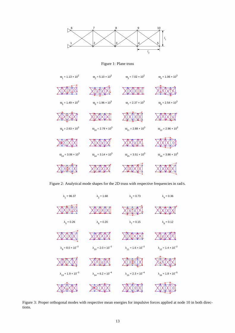
In order to explore the ideas expressed earlier, we have chosen to perform the KL expansion on a plane truss depicted in

Fig. 1.

5.1 Mode shapes determination

The truss was modelled by the finite element method using simple bar elements and an inconsistent mass matrix. The

vertical bar linking nodes 5 and 10 has l1 = 15 cm and the horizontal bar linking nodes 4 and 5 is l2 = 20 cm long. Cross-

sectional area for the elements is 1 cm2, mass density is 7860 kg/m3 and elastic modulus is 200 GPa. Since the truss

is clamped in its left extremity, implying that nodes 1 and 6 are fixed, we arrive at a 16 dof system, for other nodes are

capable of moving in both horizontal and vertical directions. Fig. 2 presents the truss together with its mass normalized

analytical mode shapes and respective natural frequencies.

The KL expansion was then performed for unitary impulsive forces acting on node 10 in both horizontal and vertical

directions. The response was measured at all 8 nodes in both directions. The time sampling rate was 0.1s which is slightly

greater than the first natural period for a reason that will be later explained, and the time span was from 0 to 100s, so

that 1000 time samples were available. Since the FEM discretization generated a system with a small number of degrees

of freedom, it is ideal for the application of the direct method. The eigenvalue problem was solved through the singular

value decomposition, for this is a robust technique that avoids numerical instabilities in the eigenvalue problem solution

that may appear due to the optimality property of the expansion. Fig. 3 presents the resulting POMs obtained from the

correlation matrix R as in Eq. (19), as well as the respective POVs expressed as a percentage of the total energy.

Since the global mass matrix of the discretized model is not proportional to the identity matrix, it is not possible to say

that the POMs are converging to the analytical mode shapes. However, it is clear that at least qualitatively, the POMs rep-

resent these mode shapes very well. Naturally, we could have multiplied the correlation matrix by the global mass matrix

in order to obtain the adjusted correlation matrix R and then calculate its eigenvectors. This was not performed because

one of the objectives here is to verify whether the POMs obtained directly from R can be taken as a good approximation

for the discretized model mode shapes. Moreover, the mode shapes for a physical structure are the eigenfunctions of an

Hermitian operator (the stiffness operator), and therefore are mutually orthogonal. Hence, the POMs from R are probably

a better representation for the real mode shapes than those calculated from the discretized model.

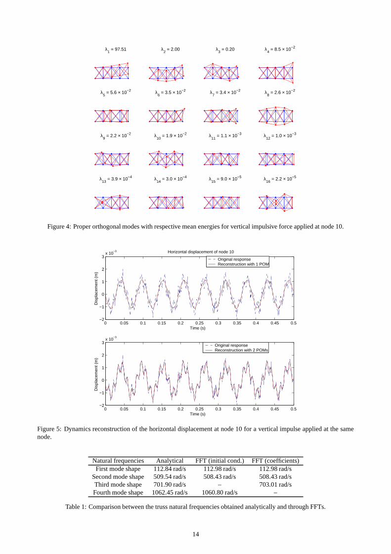
Fig. 4 presents the resulting POMs from a vertical impulse applied at the same node 10. In this case, there was an

increase in the energy contained in the first POM and in the remaining pure flexural modes such as the second, third, and

7

tenth POMs, when compared to the previous case. Furthermore, there were some difficulties in the representation of some

mode shapes. The ninth POM, for example, is a poor representation of the fourteenth mode shape and the fifth POM is

completely distinct from any of the mode shapes. This result is a consequence of the small excitation provided to some

modes due to the restriction of the excitation force to one single direction.

The optimality property of the KL expansion is clearly demonstrated in Fig. 5 where the reconstruction of the hori-

zontal displacement of node 10 is performed using the first one and the first two POMs presented in Fig. 4 which account

for 97.5% and 99.5%, respectively, of the total energy. One can observe that these first two modes suffice for a good

dynamics representation.

On the other hand, this same optimality property means that this is a noncausal procedure where the empirical modes

cannot be determined before the system response is known. Moreover, changing the impulse excitation direction will

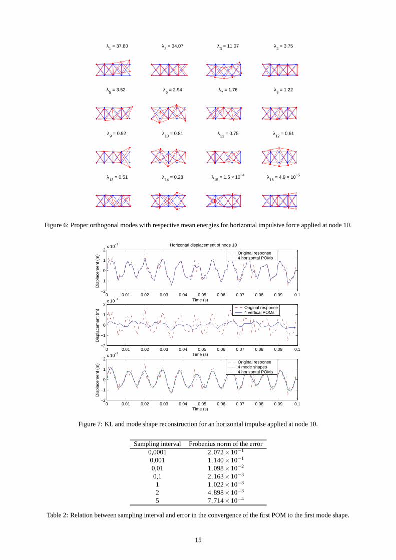
result in a completely different energy distribution among the POMs. Fig. 6 shows the POMs obtained for a horizontal

impulse applied at node 10.

In this case, we have a more homogeneous energy distribution where the first POM accounts for only 37.8% of it. This

results in a necessity of using a greater number of POMs to accomplish an accurate dynamics representation. The first

graph in Fig. 7 depicts the same horizontal displacement of node 10 used in the former case. One can note that even using 4

POMs, a good representation is not attained. This happens because for the dynamics resulting from the horizontal impulse

application, the first four POMs respond for only 87% of the energy, far from the 99% threshold usually recommended

[12]. The dynamics reconstruction is even worse if one attempts to use the first four POMs obtained from the vertical

impulse excitation (Fig. 4), as shown in the second graph. Although in that former case these four POMs accounted for

more than 99% of the energy, this is not true for the dynamics resulting from the horizontal impulse. Comparing Figs. 4

and 6, one notes that for the present case, those four POMs represent less than 50% of the energy and thus are unable to

accurately represent the horizontal displacement of node 10. Therefore, it is possible to conclude that the KL expansion

may not be robust enough to generate a reduced-order model when excitation conditions change dramatically.

The third graph also presents a modal reconstruction using the first four analytical mode shapes. The result is not

bad because the first three mode shapes correspond qualitatively to the first 3 POMs obtained for the horizontal impulse.

Another reconstruction was then performed in the same graph using POMs one, two, three and six which are related to

the first four mode shapes. One can observe that this representation is practically indistinguishable from the modal one.

However, the evaluation of the error norm error between both reconstructions and the original response yields 4,90×10−3

for the modal case and 4,61× 10−3 for these POMs. This is an interesting result and demonstrates once again how the

optimality property works in order to provide empirical modes that better represent the sampled dynamics.

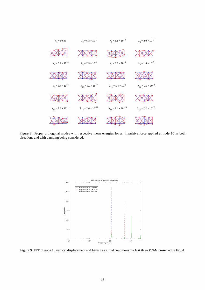
Finally, the effect of structural damping was investigated. Damping was introduced in the system of second-order

ODEs through a damping matrix which was proportional to the stiffness matrix, that is C = βK, where β = 1×10−4. This

proportional damping corresponds to modal damping factors ranging from ζ1 = 0.0057 to ζ16 = 0.1930 according to the

relation ζi = βωi/2. The truss was once again excited by means of impulsive forces acting on node 10 in both directions

and the same sampling conditions were observed. The POMs obtained with the KL expansion for this case are presented

in Fig. 8.

It is clear that the presence of proportional damping had the effect of concentrating the energy in the first POM

8

because the first mode shape has the smallest damping factor. Moreover, damping made it more difficult for some POMs

to approximate the respective mode shapes.

5.2 Natural frequencies determination

So far nothing has been mentioned about how to obtain the system natural frequencies from the KL expansion. At a

first glance, the expansion provides only the mode shapes, in the case of linear systems. However, this drawback can be

overcome by using the POMs as initial conditions and performing a Fast Fourier Transform of the resulting dynamical

response. Hence, the first three POMs depicted in Fig. 4 and that correspond to the first, second, and fourth mode shapes

were given as initial conditions to the truss in three distinct occasions. The vertical displacement of node 10 was then

sampled in 0.001s steps until 1s and the FFT of this signal performed. The result is presented in Fig. 9 where the natural

frequencies characteristic peaks for these mode shapes are clearly visible.

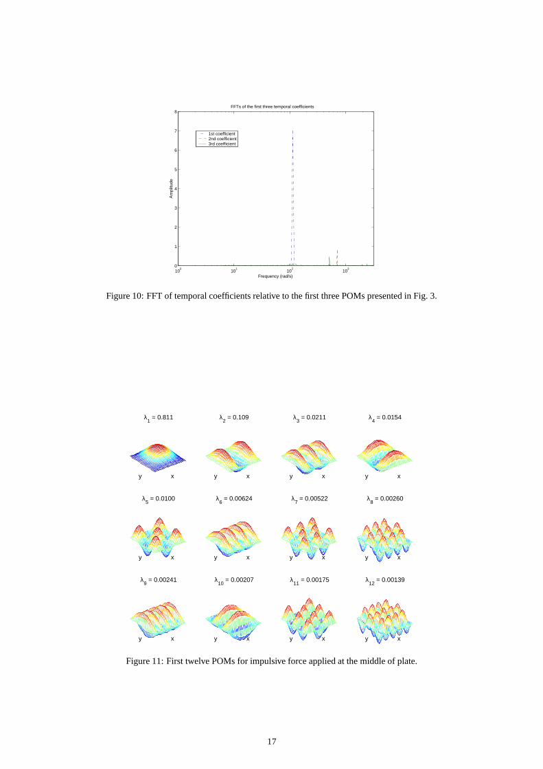
Nonetheless, in the real world, it is usually not realizable to give a certain spatial form to a structure. A more straight-

forward strategy for finding the natural frequencies is to perform a FFT of the temporal coefficients (also called principal

coordinates) of the expansion (8) as, in the linear case, they correspond to the modal amplitudes. Fig. 10 presents the

results of the FFT performed on the temporal coefficients calculated from the dynamics projection onto the first three

POMs, according to Eq. (9). These POMs appear in Fig. 3 and correspond to the first, third and second mode shapes.

Once again, the respective natural frequencies peaks are clearly visible. Table 1 compares the natural frequencies obtained

using the FFT through both methods with the analytical natural frequencies. An excellent agreement is observed.

6 Dynamics of a uniform rectangular simply supported plate

The equation of free motion for such a plate of dimensions a×b is [5]:

DE ∇4w(x, t)+ρ∂2w(x, t)

∂t2 = 0; DE =Eh3

12(1−ν2), (22)

where x = (x,y) and with the following mode shapes and natural frequencies:

wmn(x,y) =2

√

ρabsin

mπxa

sinnπy

b; ωmn = π2

√

DE

ρ

[

(ma

)2+

(nb

)2]

, (23)

satisfying the orthogonality condition

� a

0

� b

0ρwmn(x,y)wkl(x,y)dxdy = ρ

� a

0

� b

0wmn(x,y)wkl(x,y)dxdy = δmn,kl . (24)

Thus, the plate dynamics for zero initial conditions and an unitary impulsive force applied at x = f1 × a and y = f2 × b,

where f1 ∈ [0,1], f2 ∈ [0,1], is given by

w(x,y, t) =∞

∑m=1

∞

∑n=1

4ρab

sin( f1mπ)sin( f2nπ)

ωmnsin

mπxa

sinnπy

bsinωmnt. (25)

9

7 Application of the KL decomposition to the dynamics of a simply supported

plate

A distributed-parameter system such as this can be viewed as a natural extension of a discrete system with the number of

modes tending to infinity. Indeed, since the independent mode shapes for the plate are known, the orthogonality relation

Eq. (24) is equivalent to a discrete system with a mass matrix proportional to the identity matrix. Hence, it is expected that

the spatial correlation matrix eigenvectors found through the direct method will converge to the analytical mode shapes.

As an example, an impulsive force was applied to the middle ( f1 = f1 = 1/2) of a retangular (a = 1.9m, b = 1m)

steel plate 5mm thick. In order to compute the analytical response, 256 mode shapes were employed. These particular

dimensions assure us that there are no repeated natural frequencies. The spatial domain was discretized in a grid with

points spaced by 0.05m. The response was sampled using a 1s time interval (this will be later discussed) which is slightly

greater than the first mode oscillation period. The resulting POMs were computed and are shown in Fig. 11. One thousand

time samples were needed to attain these results. Notice also that the POVs are normalized, so that their sum is one.

Although the results are good, it is clear that no mode shape with m or n even was encountered. That is, naturally,

due to the position of the impulsive force. Mode shapes with a node in the middle of the plate would not be excited and,

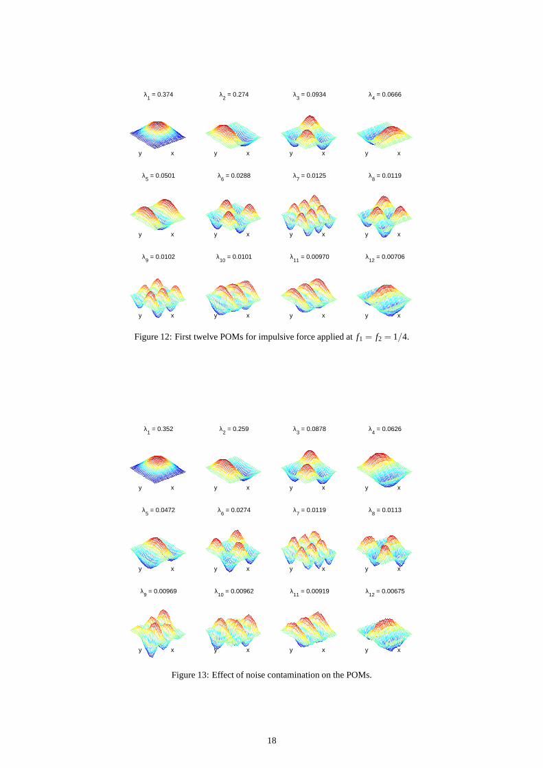
thus, do not appear in the statistically determined POMs. Shifting the force application point to f1 = f2 = 1/4 yields the

new POMs depicted in Fig. 12. It is possible to observe some new even mode shapes and the fact that the energy is less

concentrated in the first POM.

Shifting the force far away from the center affects negatively the results since the most excited mode shapes are high

frequency ones that are seldom of interest. Furthermore, the number of time samples to achieve convergence increases

a lot. Fortunately, in a physical experiment, the singularity present in the application of a numerical impulse would be

avoided and there should be no difficulty in obtaining low frequencies mode shapes through the use of an impact hammer

around the center of the plate.

The robustness of the procedure to noise was also investigated. The data were contaminated by addition of gaussian

white noise. The procedure consisted in summing the exact response to numeric generated gaussian white noise previously

to calculating the POMs. However, these proved to be quite insensitive to noise. Only when the signal to noise ratio was

of O(10) was there noticeable qualitative change in the POMs as shown in Fig. 13. Even then, the mode shapes are clearly

recognizable in the POMs. However, this level of noise is quite high and not to be expected in experimental setups. In

this example, the impulsive force was also applied at f1 = f2 = 1/4.

The time span of 1000s used so far is rather unrealistic since structural damping will always be present and because of

that, free plate vibrations will not be sustained for so long. As mentioned previously, if a structure is lightly damped, then

it should be possible to find its mode shapes through the KL decomposition. The presence of damping and consequent

decrease in available time span and the necessity of a great number of snapshots or time samples to attain convergence

would mean decreasing dramatically the sampling interval. On the other hand, the ergodicity assumption used so far

implies the use of uncorrelated snapshots. But we are actually dealing with a deterministic system, meaning that this

would, indeed, be impossible. Choosing the sampling time of 1s (above the first period) was a strategy to minimize this

problem. Results showed that increasing the sampling time above this threshold made no difference but decreasing it did.

10

Introducing a modal damping factor ζmn = 0.01 and sampling the plate dynamics in 0.001 steps until 1s (giving the same

1000 samples) produces the POMs depicted in Fig. 14. Table 2 also presents the Frobenius norm of the difference between

the first POM and the first plate mode shape for different sampling intervals and considering the undamped case. It is

clear that the error monotonically decreases when the interval is increased until past the first natural period. From then on,

there is no established pattern and the error seems to oscillate around the value associated with the first period. Therefore,

it is logical to conclude that decreasing sampling time to deal with damping is not a good strategy. Perhaps a better option,

specially in an experimental case, would be to apply another impulsive force after some time, thus increasing the available

time span for measurements.

Finally, the behavior of a square plate was investigated. This system has infinite pairs of equal frequencies. It was

excited by means of an unitary impulse applied to its center. The time span was 1000s sampled at every second. The

first four resulting POMs are presented in Fig. 15. It is interesting to note that the KL decomposition was unable to

differentiate between mode shapes having the same frequency. Because they are vibrating in phase, statistically they

cannot be distinguished and end up added by the procedure. One result, for instance, is the second POM which is, in

reality, the sum of mode shapes w13(x,y)+w31(x,y). And the fourth POM is the result of w15(x,y)+w51(x,y) (note that

the even modes do not appear due to the applied impulse position, as discussed earlier).

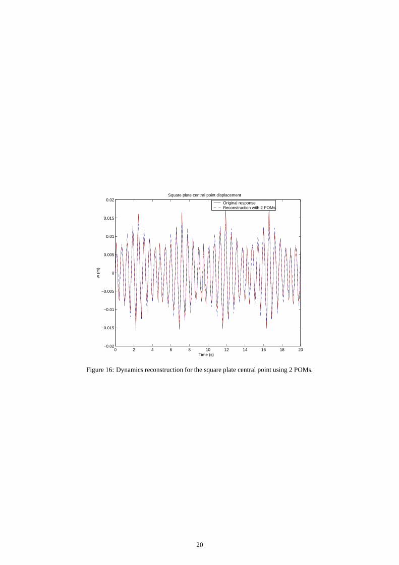
This is a great disadvantage for performing modal analysis in unknown systems via the KL decomposition. However,

if the objective is to construct a reduced-order model, the method continues to be optimal. Using only the first two POMs,

it is possible to practically reconstruct the original dynamics for the plate central point as can be seen in Fig. 16.

8 Conclusions

This worked discussed the use of the Karhunen-Loeve expansion as a tool to perform modal analysis of distributed-

parameter linear system. It was shown that the proper orthogonal modes obtained with the procedure are a good approx-

imation for the analytical mode shapes of a discretized model with diagonal global mass matrix. A great advantage of

using the KL expansion for modal analysis is that the proper orthogonal values provide the contribution of the associated

POMs in the global dynamics. Moreover, it was also demonstrated that the convergence capacity of the expansion is little

affected by the existence of gaussian noise.

Nevertheless, there are also some disadvantages in its application. First of all, the sampling time should be at least

close to the first oscillation period, what possibly will not be know a priori in an experimental case. And only lightly

damped structures can be the object of analysis by this method. Besides that, the expansion cannot differentiate mode

shapes with the same frequency which end up added. Finally, there is also the necessity of measuring the structure

dynamical response in a fairly large number of points.

Therefore, although it is possible that the Karhunen-Loeve expansion may replace traditional modal analysis in some

applications, it is for now more likely that it will be used as an additional tool, specially when choosing a modal basis for

a reduced order model, due to its optimality property.

11

9 Acknowledgment

The first author gratefully acknowledges the financial support provided by Brazilian “Fundacao Carlos Chagas Filho de

Amparo a Pesquisa do Estado do Rio de Janeiro” (FAPERJ) through a graduate scholarship, grant No. E-26/150.687/2000.

References

[1] Breuer, K.S. and Sirovich, L. The use of the Karhunen-Loeve procedure for the calculation of linear eigenfunctions.

Journal of Computational Physics, 96:277–296, 1991.

[2] Feeny, L. and Kappagantu, R. On the physical interpretation of proper orthogonal modes in vibrations. Journal of

Sound and Vibration, 211(4):607–616, 1998.

[3] Hochstadt, H. Integral equations. John Wiley & Sons, 1989.

[4] Holmes, P., Lumley, J.L., and Berkooz, G. Turbulence, coherent structures, dynamical systems and symmetry.

Cambridge University Press, 1996.

[5] Inman, D.J. Engineering vibration. Prentice-Hall, 1996.

[6] Kreuzer, E. and Kust, O. Analysis of long torsional strings by proper orthogonal decomposition. Archive of Applied

Mechanics, 67:68–80, 1996.

[7] Lumley, J.L. Stochastic tools in turbulence. Academic Press, 1971.

[8] Ma, X. and Vakakis, A.F. Karhunen-Loeve decomposition of the transient dynamics of a multibay truss. AIAA

Journal, 37(8):939–946, 1999.

[9] Meirovitch, L. Principles and techniques of vibrations. Prentice-Hall, 1997.

[10] Newman, A.J. Model reduction via the Karhunen-Loeve expansion part I: an exposition. Technical report 96-32,

Institute for Systems Research, 1996.

[11] Papoulis, A. Probablity, random variables, and stochastic processes. McGraw-Hill, 1991.

[12] Sirovich, L. Turbulence and the dynamics of coherent structures part I: coherent structures. Quarterly of Applied

Mathematics, 45(3):561–571, 1987.

[13] Sirovich, L. Turbulence and the dynamics of coherent structures part II: symmetries and transformations. Quarterly

of Applied Mathematics, 45(3):573–582, 1987.

[14] Sirovich, L. Turbulence and the dynamics of coherent structures part III: dynamics and scaling. Quarterly of

Applied Mathematics, 45(3):583–590, 1987.

[15] Steindl, A., Troger, H., and Zemann, J.V. Nonlinear Galerkin methods applied in the dimension reduction of vibrat-

ing fluid conveying tubes. In Paidoussis, M.P., Bajaj, A.K., Corke, T.C., Farabee, T.M., and Williams, F. Hara D.R.,

eds., ASME Symposium on Fluid-Structure Interaction, Aeroelasticity, Flow-Induced Vibration and Noise, ASME,

Dallas, EUA, vol. AD53-1, pp. 273–280, 1997.

12

1 2 3 4 5

6 7 8 9 10

l 1

l 2

Figure 1: Plane truss

ω1 = 1.13 × 102 ω

2 = 5.10 × 102 ω

3 = 7.02 × 102 ω

4 = 1.06 × 103

ω5 = 1.49 × 103 ω

6 = 1.96 × 103 ω

7 = 2.37 × 103 ω

8 = 2.54 × 103

ω9 = 2.63 × 103 ω

10 = 2.79 × 103 ω

11 = 2.88 × 103 ω

12 = 2.96 × 103

ω13

= 3.06 × 103 ω14

= 3.14 × 103 ω15

= 3.51 × 103 ω16

= 3.86 × 103

Figure 2: Analytical mode shapes for the 2D truss with respective frequencies in rad/s.

λ1 = 96.37 λ

2 = 1.68 λ

3 = 0.73 λ

4 = 0.36

λ5 = 0.26 λ

6 = 0.20 λ

7 = 0.15 λ

8 = 0.12

λ9 = 8.0 × 10−2 λ

10 = 2.0 × 10−2 λ

11 = 1.6 × 10−2 λ

12 = 1.4 × 10−2

λ13

= 1.9 × 10−3 λ14

= 6.2 × 10−4 λ15

= 2.3 × 10−4 λ16

= 1.8 × 10−5

Figure 3: Proper orthogonal modes with respective mean energies for impulsive forces applied at node 10 in both direc-tions.

13

λ1 = 97.51 λ

2 = 2.00 λ

3 = 0.20 λ

4 = 8.5 × 10−2

λ5 = 5.6 × 10−2 λ

6 = 3.5 × 10−2 λ

7 = 3.4 × 10−2 λ

8 = 2.6 × 10−2

λ9 = 2.2 × 10−2 λ

10 = 1.9 × 10−2 λ

11 = 1.1 × 10−3 λ

12 = 1.0 × 10−3

λ13

= 3.9 × 10−4 λ14

= 3.0 × 10−4 λ15

= 9.0 × 10−5 λ16

= 2.2 × 10−5

Figure 4: Proper orthogonal modes with respective mean energies for vertical impulsive force applied at node 10.

0 0.05 0.1 0.15 0.2 0.25 0.3 0.35 0.4 0.45 0.5−2

−1

0

1

2

3x 10

−3 Horizontal displacement of node 10

Time (s)

Dis

plac

emen

t (m

)

Original responseReconstruction with 1 POM

0 0.05 0.1 0.15 0.2 0.25 0.3 0.35 0.4 0.45 0.5−2

−1

0

1

2

3x 10

−3

Time (s)

Dis

plac

emen

t (m

)

Original responseReconstruction with 2 POMs

Figure 5: Dynamics reconstruction of the horizontal displacement at node 10 for a vertical impulse applied at the samenode.

Natural frequencies Analytical FFT (initial cond.) FFT (coefficients)First mode shape 112.84 rad/s 112.98 rad/s 112.98 rad/s

Second mode shape 509.54 rad/s 508.43 rad/s 508.43 rad/sThird mode shape 701.90 rad/s – 703.01 rad/sFourth mode shape 1062.45 rad/s 1060.80 rad/s –

Table 1: Comparison between the truss natural frequencies obtained analytically and through FFTs.

14

λ1 = 37.80 λ

2 = 34.07 λ

3 = 11.07 λ

4 = 3.75

λ5 = 3.52 λ

6 = 2.94 λ

7 = 1.76 λ

8 = 1.22

λ9 = 0.92 λ

10 = 0.81 λ

11 = 0.75 λ

12 = 0.61

λ13

= 0.51 λ14

= 0.28 λ15

= 1.5 × 10−4 λ16

= 4.9 × 10−5

Figure 6: Proper orthogonal modes with respective mean energies for horizontal impulsive force applied at node 10.

0 0.01 0.02 0.03 0.04 0.05 0.06 0.07 0.08 0.09 0.1−2

−1

0

1

2x 10

−3 Horizontal displacement of node 10

Time (s)

Dis

plac

emen

t (m

) Original response4 horizontal POMs

0 0.01 0.02 0.03 0.04 0.05 0.06 0.07 0.08 0.09 0.1−2

−1

0

1

2x 10

−3

Time (s)

Dis

plac

emen

t (m

) Original response4 vertical POMs

0 0.01 0.02 0.03 0.04 0.05 0.06 0.07 0.08 0.09 0.1−2

−1

0

1

2x 10

−3

Time (s)

Dis

plac

emen

t (m

) Original response4 mode shapes4 horizontal POMs

Figure 7: KL and mode shape reconstruction for an horizontal impulse applied at node 10.

Sampling interval Frobenius norm of the error0,0001 2,072×10−1

0,001 1,140×10−1

0,01 1,098×10−2

0,1 2,163×10−3

1 1,022×10−3

2 4,898×10−3

5 7,714×10−4

Table 2: Relation between sampling interval and error in the convergence of the first POM to the first mode shape.

15

λ1 = 99.88 λ

2 = 6.3 × 10−2 λ

3 = 5.1 × 10−2 λ

4 = 2.0 × 10−3

λ5 = 5.2 × 10−4 λ

6 = 2.3 × 10−4 λ

7 = 8.3 × 10−5 λ

8 = 1.6 × 10−5

λ9 = 6.7 × 10−6 λ

10 = 8.0 × 10−7 λ

11 = 5.4 × 10−8 λ

12 = 2.9 × 10−9

λ13

= 3.4 × 10−11 λ14

= 2.6 × 10−12 λ15

= 1.4 × 10−14 λ16

= 2.2 × 10−15

Figure 8: Proper orthogonal modes with respective mean energies for an impulsive force applied at node 10 in bothdirections and with damping being considered.

100

101

102

103

0

50

100

150

200

250

300

Frequency (rad/s)

Am

plitu

de

FFT of node 10 vertical displacement

Initial condition: 1st POMInitial condition: 2nd POMInitial condition: 3rd POM

Figure 9: FFT of node 10 vertical displacement and having as initial conditions the first three POMs presented in Fig. 4.

16

100

101

102

103

0

1

2

3

4

5

6

7

8

Frequency (rad/s)

Am

plitu

de

FFTs of the first three temporal coefficients

1st coefficient2nd coefficient3rd coefficient

Figure 10: FFT of temporal coefficients relative to the first three POMs presented in Fig. 3.

x

λ1 = 0.811

y x

λ2 = 0.109

y x

λ3 = 0.0211

y x

λ4 = 0.0154

y

x

λ5 = 0.0100

y x

λ6 = 0.00624

y x

λ7 = 0.00522

y x

λ8 = 0.00260

y

x

λ9 = 0.00241

y x

λ10

= 0.00207

y x

λ11

= 0.00175

y x

λ12

= 0.00139

y

Figure 11: First twelve POMs for impulsive force applied at the middle of plate.

17

x

λ1 = 0.374

y x

λ2 = 0.274

y x

λ3 = 0.0934

y x

λ4 = 0.0666

y

x

λ5 = 0.0501

y x

λ6 = 0.0288

y x

λ7 = 0.0125

y x

λ8 = 0.0119

y

x

λ9 = 0.0102

y x

λ10

= 0.0101

y x

λ11

= 0.00970

y x

λ12

= 0.00706

y

Figure 12: First twelve POMs for impulsive force applied at f1 = f2 = 1/4.

x

λ1 = 0.352

y x

λ2 = 0.259

y x

λ3 = 0.0878

y x

λ4 = 0.0626

y

x

λ5 = 0.0472

y x

λ6 = 0.0274

y x

λ7 = 0.0119

y x

λ8 = 0.0113

y

x

λ9 = 0.00969

y x

λ10

= 0.00962

y x

λ11

= 0.00919

y x

λ12

= 0.00675

y

Figure 13: Effect of noise contamination on the POMs.

18

x

λ1 = 0.425

y x

λ2 = 0.281

y x

λ3 = 0.0934

y x

λ4 = 0.0617

y

x

λ5 = 0.0478

y x

λ6 = 0.0249

y x

λ7 = 0.0150

y x

λ8 = 0.00904

y

x

λ9 = 0.00818

y x

λ10

= 0.00775

y x

λ11

= 0.00534

y x

λ12

= 0.00285

y

Figure 14: Effect of reducing sample time on POMs

λ1 = 0.887 λ

2 = 0.0707

λ3 = 0.0110 λ

4 = 0.0105

Figure 15: POMs for square plate. Impulsive force applied at the center.

19

0 2 4 6 8 10 12 14 16 18 20−0.02

−0.015

−0.01

−0.005

0

0.005

0.01

0.015

0.02

Time (s)

w (

m)

Square plate central point displacement

Original responseReconstruction with 2 POMs

Figure 16: Dynamics reconstruction for the square plate central point using 2 POMs.

20