KATHOLIEKE UNIVERSITEIT LEUVEN FACULTEIT INGENIEURSWETENSCHAPPEN DEPARTEMENT ELEKTROTECHNIEK Kasteelpark Arenberg 10, 3001 Leuven (Heverlee) THE APPLICATION OF PROPER ORTHOGONAL DECOMPOSITION TO THE CONTROL OF TUBULAR REACTORS Promotor : Prof. dr. ir. B. De Moor Co-Promotors : Prof. dr. ir. J. Espinosa Prof. dr. ir. J. Vandewalle Proefschrift voorgedragen tot het behalen van het doctoraat in de ingenieurswetenschappen door Oscar Mauricio AGUDELO November 2009

Welcome message from author
This document is posted to help you gain knowledge. Please leave a comment to let me know what you think about it! Share it to your friends and learn new things together.
Transcript
KATHOLIEKE UNIVERSITEIT LEUVEN
FACULTEIT INGENIEURSWETENSCHAPPEN
DEPARTEMENT ELEKTROTECHNIEK
Kasteelpark Arenberg 10, 3001 Leuven (Heverlee)
THE APPLICATION OF PROPER ORTHOGONAL
DECOMPOSITION TO THE CONTROL OF TUBULAR
REACTORS
Promotor :
Prof. dr. ir. B. De Moor
Co-Promotors :
Prof. dr. ir. J. Espinosa
Prof. dr. ir. J. Vandewalle
Proefschrift voorgedragen tot
het behalen van het doctoraat
in de ingenieurswetenschappen
door
Oscar Mauricio AGUDELO
November 2009

KATHOLIEKE UNIVERSITEIT LEUVEN
FACULTEIT INGENIEURSWETENSCHAPPEN
DEPARTEMENT ELEKTROTECHNIEK
Kasteelpark Arenberg 10, 3001 Leuven (Heverlee)
THE APPLICATION OF PROPER ORTHOGONAL
DECOMPOSITION TO THE CONTROL OF TUBULAR
REACTORS
Jury:
Prof. dr. ir. Y. Willems, voorzitter
Prof. dr. ir. B. De Moor, promotor
Prof. dr. ir. J. Espinosa, co-promotor (UNAL)
Prof. dr. ir. J. Vandewalle, co-promotor
Prof. dr. ir. J. Suykens
Prof. dr. ir. J. Van Impe
Prof. dr. ir. A.C.P.M. Backx (TU/e)
Prof. dr. ir. I. Smets
Proefschrift voorgedragen tot
het behalen van het doctoraat
in de ingenieurswetenschappen
door
Oscar Mauricio AGUDELO
November 2009

c©Katholieke Universiteit Leuven – Faculteit IngenieurswetenschappenArenbergkasteel, B-3001 Heverlee (Belgium)
Alle rechten voorbehouden. Niets uit deze uitgave mag vermenigvuldigden/of openbaar gemaakt worden door middel van druk, fotocopie, microfilm,elektronisch of op welke andere wijze ook zonder voorafgaande schriftelijketoestemming van de uitgever.
All rights reserved. No part of the publication may be reproduced in anyform by print, photoprint, microfilm or any other means without writtenpermission from the publisher.
ISBN 978-94-6018-133-7
D/2009/7515/116

To my mother Luz Marina, my greatest teacher


Foreword
This thesis is the product of my research activities during my doctoralstudies at the SCD/SISTA research division of the Electrical EngineeringDepartment of the Katholieke Universiteit Leuven. It has been an incrediblejourney of learning, full of challenges and nice experiences where I have notonly grown as researcher but also as human being.
I want to thank my promotor Prof. Bart De Moor for his continuous supportand guidance along my doctoral studies. I am also very grateful to my co-promotor Prof. Joos Vandewalle, who gave me the opportunity to join theresearch group as a predoctoral student. My gratitude goes as well to my co-promotor Prof. Jairo Espinosa, for his unconditional assistance, guidanceand constant feedback since I was finishing my master studies in Ibague,Colombia. I also want to thank Prof. Moritz Diehl and Dr. Michel Baes,for playing an important role during part of my research. I have to say thatworking together with them has been a very enriching experience for me.Many thanks to Prof. Johan Suykens, Prof. Jan Van Impe, Prof. Ton Backxand Prof. Ilse Smets for being part of the jury of this thesis. I would like toacknowledge the help that I received from the administrative staff, namelyIda Tassens and Ilse Pardon during all these years. I extend my gratitudeto all my colleagues and friends, who made this journey a memorable andenjoyable experience.
Furthermore, I want to express my gratitude to all the people that in one wayor another have made my stay in Belgium quite pleasant. Especially I wantto thank Jairo Espinosa and his nice family, for considering me as anotherfamily member and for making me feel like at home. From the deepestpart of my heart, Jairo, Claudia, Laurita, Jairito, Don Jairo and Dona alba,thank you to all of you. At the end of my second Ph.D year I had to undergoa knee surgery, and it was a quite tough moment for me. At that point I
i

ii
have to say that the moral support of my family from Colombia and thehelp of Don Jairo in Belgium allowed me to go through. Many thanks DonJairo for your unconditional support, hospitality and friendship.
Last but not least, I want to thank my mother Luz Marina, my father LuisOscar, my brother Jorge Ernesto and my sister Carolina, for accompanyingme from the distance in this journey, and for cheering me up in the mostdifficult times. Gracias madre, por ser la luz que Dios puso a mi lado parano extraviar el camino.
Oscar Mauricio Agudelo Manozca
Leuven, November 2009.

Abstract
This dissertation considers two main research topics. First, this thesisexplores the applicability of Proper Orthogonal Decomposition (POD) andGalerkin projection in the design of Model Predictive Control (MPC)schemes for tubular chemical reactors. These processes pose very interestingcontrol problems, since their behavior is modeled by highly nonlinear PartialDifferential Equations (PDEs), and they require the satisfaction of boththeir input (physical limitation of the actuators) and state constraints (e.g.,the temperature inside the reactor must be below a given value in order toavoid the formation of byproducts). In this study, POD is used together withGarlerkin projection for reducing the high-dimensionality of the discretizedsystems used to approximate the PDEs that model the reactors. Then,based on the resulting reduced-order models, Kalman filters and predictivecontrollers are designed. Although a significant model order reduction canbe obtained with POD and Galerkin projection, these techniques do notreduce the number of state constraints (linear inequality constraints) whichis typically very large. In this thesis we propose two methods to tackle thisproblem. In the first method we use univariate polynomials to approximatepart of the basis vectors derived with the POD technique, and then we applythe theory of positive polynomials to find good approximations of the stateconstraints by Linear Matrix Inequalities (LMIs). In the second method,we exploit the similarities between the coefficients of consecutive stateconstraints for developing a greedy algorithm that selects a small numberof constraints from the complete set. This algorithm reduces dramaticallythe number of state constraints, and consequently the memory needed forstoring them and the time required for solving the optimization problem.
The second main research subject of this thesis is related to speeding upthe evaluation of reduced-order models derived by POD from nonlinearhigh-dimensional systems. Unlike the Linear Time Invariant (LTI) case,
iii
iv
the model-order reduction by POD and Galerkin projection does notconduce to an important computational saving when the high-dimensionalmodels under consideration are nonlinear or Linear Time Variant (LTV).Therefore, this thesis introduces two methods for coping with this situation.The first method takes advantage of the input-output nonlinear mappingcapabilities, and the fast on-line evaluation of Multi-Layer Perceptrons(MLPs) for accelerating the evaluation of the POD models. The secondmethod exploits the polynomial nature of POD models derived from input-affine high-dimensional systems with polynomial nonlinearities, in order togenerate compact and efficient formulations that can be evaluated muchfaster. Moreover, in this study it is shown how the use of sequential featureselection algorithms can provide a significant boost in the computationalsaving. Although this method is not as general as the first one, it mightbe applied to models with non-polynomial nonlinearities, provided that thenonlinearities can be approximated by low degree polynomials. In addition,conditions for guaranteeing the local stability of these POD models withpolynomial nonlinearities are discussed.

Notation
Variables and Symbols
xT Transpose of the vector xAT Transpose of the matrix AAij or A(i, j),A ∈ R
m×n Element at the ith row and jth column of AA(i, :),A ∈ R
m×n ith row of AA(:, j),A ∈ R
m×n jth column of AAH Conjugate transpose of the matrix AIn Identity matrix of size n × nI Identity matrix‖x‖2, x ∈ R
n L2-norm or Euclidean norm of a vector :√
xTx‖x‖Q, x∈ R
n,Q∈ Rn×n Weighted norm:
√xTQx
〈x,y〉, x,y ∈ Rn Euclidean inner product between two vectors:
xTy = yTx[x; z],x, z ∈ R
n Stacked vectors : [xT , zT ]T ∈ R2n
{xi}pi=1 Data set with p elements : {x1,x2, . . . ,xp}
1 Vector where all components are equal to 1
v

vi
Acronyms
ARE Algebraic Riccati EquationBDS Bidirectional SearchBMI Bilinear Matrix InequalityCTR Continuous Tubular ReactorCSTR Continuous Stirred-Tank ReactorKLD Karhunen-Loeve DecompositionLMI Linear Matrix InequalityLTI Linear Time InvariantLTV Linear Time VariantLRS Plus-L Minus-R SelectionMEMS Micro-Electro-Mechanical SystemMLP Multi-Layer PerceptronMPC Model Predictive ControlMPE Missing Point EstimationMSE Mean Squared ErrorNSDP Nonlinear SemiDefinite Program or ProgrammingODE Ordinary Differential EquationPCA Principal Component AnalysisPDE Partial Differential EquationPFR Plug Flow ReactorPOD Proper Orthogonal DecompositionPOM Proper Orthogonal ModePOV Proper Orthogonal ValueP-POD Polynomial POD modelPRBNS Pseudo Random Binary Noise SignalsPRMNS Pseudo Random Multilevel Noise SignalsQP Quadratic Programming or ProgramRHC Receding Horizon ControlSBS Sequential Backward SelectionSDP SemiDefinite Program or ProgrammingSFS Sequential Forward SelectionSOS Sum Of SquaresSQP Sequential Quadratic ProgrammingSSE Sum Squared ErrorSVD Singular Value Decomposition

Contents
Foreword i
Abstract iii
Notation v
Contents vii
1 General Introduction 1
1.1 Introduction and motivation . . . . . . . . . . . . . . . . . . . 1
1.2 Objectives . . . . . . . . . . . . . . . . . . . . . . . . . . . . . 5
1.3 Chapter by chapter overview . . . . . . . . . . . . . . . . . . 5
1.4 Contribution of this thesis . . . . . . . . . . . . . . . . . . . . 9
2 Proper Orthogonal Decomposition and Predictive Control 13
2.1 Introduction . . . . . . . . . . . . . . . . . . . . . . . . . . . . 13
2.2 Proper orthogonal decomposition . . . . . . . . . . . . . . . . 14
2.2.1 General procedure . . . . . . . . . . . . . . . . . . . . 15
2.2.2 Model reduction . . . . . . . . . . . . . . . . . . . . . 18
2.3 Model predictive control . . . . . . . . . . . . . . . . . . . . . 21
vii

viii Contents
2.3.1 Predictive control principle . . . . . . . . . . . . . . . 22
2.3.2 Estimation of the states . . . . . . . . . . . . . . . . . 24
2.4 Example: Temperature control in a one–dimensional bar . . . 27
2.4.1 Heat transfer in a one-dimensional bar . . . . . . . . . 27
2.4.2 Discretization . . . . . . . . . . . . . . . . . . . . . . . 28
2.4.3 Model reduction using POD . . . . . . . . . . . . . . . 30
2.4.4 MPC control scheme without a disturbance model . . 33
2.4.5 MPC control scheme with a disturbance model . . . . 38
2.5 Conclusions . . . . . . . . . . . . . . . . . . . . . . . . . . . . 42
3 Control of a Non-isothermal Tubular Reactor 45
3.1 Introduction . . . . . . . . . . . . . . . . . . . . . . . . . . . . 45
3.2 Tubular chemical reactor . . . . . . . . . . . . . . . . . . . . . 46
3.2.1 Plug flow reactor model . . . . . . . . . . . . . . . . . 47
3.2.2 Operating profiles . . . . . . . . . . . . . . . . . . . . 49
3.2.3 Linear model . . . . . . . . . . . . . . . . . . . . . . . 53
3.3 Model reduction using POD . . . . . . . . . . . . . . . . . . . 58
3.4 Predictive control schemes . . . . . . . . . . . . . . . . . . . . 65
3.4.1 First MPC control scheme (MPC-NTC) - Formulationin terms of the POD coefficients . . . . . . . . . . . . 65
3.4.2 Second MPC control scheme (MPC-PV) - Formula-tion in terms of physical variables . . . . . . . . . . . 67
3.5 Simulation results . . . . . . . . . . . . . . . . . . . . . . . . 70
3.5.1 Tests on a reactor with axial dispersion . . . . . . . . 83
3.6 Conclusions . . . . . . . . . . . . . . . . . . . . . . . . . . . . 91

Contents ix
4 Constraint Handling 95
4.1 Introduction . . . . . . . . . . . . . . . . . . . . . . . . . . . . 95
4.2 POD-based MPC controller with temperature constraints . . 96
4.3 Positive polynomial approach . . . . . . . . . . . . . . . . . . 99
4.3.1 Fundamentals . . . . . . . . . . . . . . . . . . . . . . . 99
4.3.2 Approximation of the temperature constraints bymeans of positive polynomials . . . . . . . . . . . . . . 102
4.3.3 Semidefinite representability of positive polynomialson an interval . . . . . . . . . . . . . . . . . . . . . . . 104
4.3.4 Simulation results . . . . . . . . . . . . . . . . . . . . 108
4.4 Greedy selection algorithm . . . . . . . . . . . . . . . . . . . 117
4.4.1 Simulation results . . . . . . . . . . . . . . . . . . . . 123
4.5 Conclusions . . . . . . . . . . . . . . . . . . . . . . . . . . . . 128
5 Performance Improvement in Model Simulation 131
5.1 Introduction . . . . . . . . . . . . . . . . . . . . . . . . . . . . 131
5.2 Nonlinear heat transfer in a one-dimensional bar . . . . . . . 133
5.3 Nonlinear POD model of the system . . . . . . . . . . . . . . 135
5.4 Acceleration of POD models by using neural networks . . . . 139
5.5 Polynomial POD models . . . . . . . . . . . . . . . . . . . . . 145
5.5.1 Calculation of the coefficients of the polynomials . . . 147
5.5.2 Reduction of the number of monomials . . . . . . . . . 149
5.6 Polynomial POD models with stability guarantee . . . . . . . 152
5.6.1 Semidefinite problem formulation . . . . . . . . . . . . 153
5.6.2 Nonlinear semidefinite problem formulation . . . . . . 154
5.6.3 Numerical example . . . . . . . . . . . . . . . . . . . . 155
x Contents
5.7 Validation and simulation results . . . . . . . . . . . . . . . . 160
5.8 Conclusions . . . . . . . . . . . . . . . . . . . . . . . . . . . . 167
6 General Conclusions 169
6.1 Concluding remarks . . . . . . . . . . . . . . . . . . . . . . . 169
6.2 Future research . . . . . . . . . . . . . . . . . . . . . . . . . . 172
Bibliography 175
Curriculum Vitae 187
Publications by the author 189

Chapter 1
General Introduction
1.1 Introduction and motivation
This thesis explores the application of a technique known as ProperOrthogonal Decomposition (POD), in the design of Model PredictiveControl (MPC) strategies for tubular chemical reactors. Additionally,this dissertation develops new methods for improving the performance insimulation of models derived by POD from nonlinear high-dimensionalsystems.
Tubular chemical reactors are distributed parameter systems that typicallyare modeled by coupled nonlinear Partial Differential Equations (PDEs)which are derived from mass and energy balance principles. One way ofaddressing the control of these infinite-dimensional systems is by approx-imating the PDEs by a large number of Ordinary Differential Equations(ODEs). Afterwards, given the high-dimensionality of the resulting systems,reduced order models are derived to make possible the control design. Figure1.1 shows this general control design framework. In this dissertation, thereduced order models are found by means of POD and Galerkin projection.Proper orthogonal decomposition is a data driven technique where asuitable set of orthonormal basis vectors are computed from simulationor experimental data. These basis vectors, which are organized in orderof relevance, capture the spatial dynamics of the original systems. Thereduced order models are obtained by projecting (Galerkin Projection) thehigh-dimensional models on the space spanned by the most relevant basis
1

2 General Introduction
vectors. The advantage of using these two techniques is the incorporation ofsimulated or experimental data as well as the existing physical relationshipsfrom the original model [64].
Model predictive control is a popular control method for handling inputand state constraints within an optimal control setting. In MPC, thecontrol actions are obtained by solving continually, on-line, a finite-horizonconstrained open-loop optimal control problem. The popularity of thisapproach resides largely in its ability to handle, among other issues, mul-tivariable interactions, constraints on controls and states, and optimizationrequirements. The use of this control strategy in tubular reactors is ofspecial interest since this control methodology has demonstrated that it canpush the plants towards their limits of performance while satisfying boththe input (constraints in the actuators) and the state constraints (e.g., thetemperature inside the reactor must be within a predefined range).
Tubular reactors typically operate under steady state conditions in orderto efficiently produce high product volumes of a consistent quality. Nev-ertheless, transient operation regimes are also used to minimize the off-spec material during transitions, when reactors are employed for producingdifferent kind of products. In this dissertation, the POD-based MPCcontrollers have the goal of rejecting the disturbances that affect the nominaloperation of the reactors, under steady state regimes. For a completeliterature review about model based control and optimization of tubularreactors, readers are referred to [95, page 43].
From the studies presented in [33–36], a general and practical framework forrobust control synthesis for transport reaction process, which also encompasstubular reactors, has been established. However, the drawback of thisframework is that it does not include the input and output constraints ofthe process under consideration. Consequently, the research efforts havebeen recently focused on the use of model predictive control strategies,which are characterized by dealing with the input and state constraintsof a process in a very natural way. Thus, predictive controllers have beendevised in [46, 133] for hyperbolic systems (convection-reaction processes,e.g., a tubular reactor where a plug-flow behavior is assumed), and in [44–46]for parabolic systems (Diffusion-reaction processes, e.g., a tubular reactorwith axial diffusion/dispersion).
The well-known success of POD in many applications for deriving reduced-order models for simulation and control purposes, motivates its use in

1.1 Introduction and motivation 3
this thesis for the development of alternative predictive control strategies(POD-based predictive control systems) for tubular chemical reactors. Asit was mentioned before, these predictive control schemes should push thereactors to their limits of performance while satisfying the input and outputconstraints.
There is however, an important aspect of the POD-based predictivecontrollers that should be addressed at the moment of their implementation:the reduction of the number of state/output constraints which typically isvery large, since it is given by the number of discretization points multipliedby the prediction horizon of the controllers. This large set of constraintsconsumes a significant amount of memory due to the large size of thematrices storing it, which by the way are not sparse. Furthermore, this largeamount of constraints increase the computational time required for solvingthe optimization problem of the MPC. Clearly, methods that can cope withthe reduction of the number of state/output constraints are necessary inorder to generate more efficient POD-based predictive controllers.
Leaving aside the topic of POD-based predictive controllers for tubularreactors, another problem that motivates this thesis is the one relatedwith the performance improvement in simulation of nonlinear reduced-ordermodels derived by means of POD and Galerkin projection. Although alarge model-order reduction can be achieved with these techniques, suchreduction does not lead to a significant computational saving when nonlinearor Linear Time Variant (LTV) models are considered. This limitation isdue to the necessity of having the full spatial information from the originalhigh-dimensional systems, at the moment of evaluating the reduced-ordermodels. In [10–12] a general method known as Missing Point Estimation(MPE) is introduced for coping with this problem. The method achievesa computational saving by conducting the Galerkin projection on somepre-selected state variables or points of the spatial domain instead of thecomplete set. The remaining state variables are estimated from the PODbasis vectors. Although it has been reported that this technique can saveconsiderable computation effort, the speeding up of nonlinear POD modelsis still an open problem that might be addressed from a different angle.Methods that exploit the nature of the nonlinearities, although more specificthan the MPE, might provide more accurate reduced-order models that canbe evaluated much faster.

4 General Introduction
“Adv
ance
d M
odel
Pre
dict
ive
Con
trol
Stra
tegi
es (M
PC
)”M
PC
cont
rolle
r PCPL
C
Tubu
lar R
eact
or
0 rr
w(
)
E RT E RT
CC
vkCe
tz
TT
vGCe
HT
Tt
z
Par
tial D
iffer
entia
l Equ
atio
ns
Mod
eled
by
Hig
h O
rder
Mod
els
1000
, 10.
000
stat
es, e
tc
Dis
cret
izat
ion
Prop
er O
rthog
onal
D
ecom
posi
tion
and
G
aler
kin
Proj
ectio
n
Allo
w th
e
desi
gn o
f
Red
uced
-ord
erM
odel
s
Tubu
lar R
eact
ors
Fig
ure
1.1:
Con
trol
desi
gnfr
amew
ork.
1.2 Objectives 5
1.2 Objectives
The main objectives of this dissertation are summarized in the followinglines.
• To explore the applicability of proper orthogonal decomposition inthe design of model predictive control schemes for tubular chemicalreactors.
• To propose methods for reducing the number of state/output con-straints of POD-based model predictive controllers.
• To derive alternative techniques for speeding up the evaluation ofnonlinear or Linear Time Variant (LTV) POD models.
1.3 Chapter by chapter overview
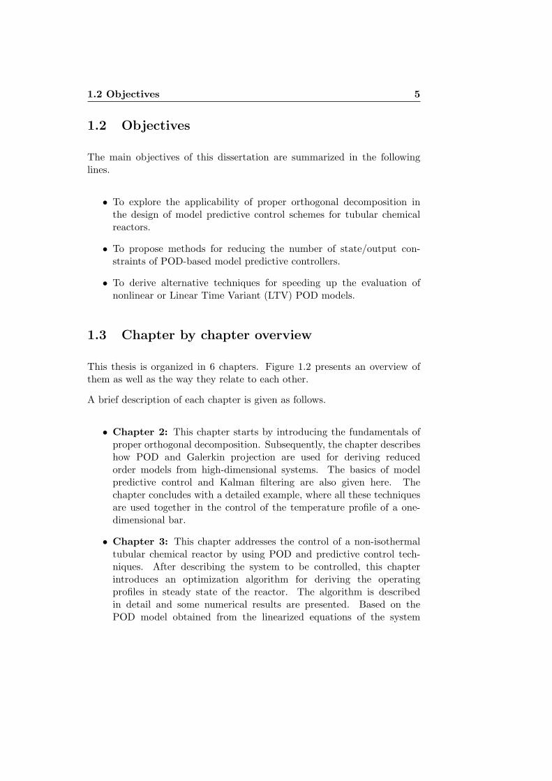
This thesis is organized in 6 chapters. Figure 1.2 presents an overview ofthem as well as the way they relate to each other.
A brief description of each chapter is given as follows.
• Chapter 2: This chapter starts by introducing the fundamentals ofproper orthogonal decomposition. Subsequently, the chapter describeshow POD and Galerkin projection are used for deriving reducedorder models from high-dimensional systems. The basics of modelpredictive control and Kalman filtering are also given here. Thechapter concludes with a detailed example, where all these techniquesare used together in the control of the temperature profile of a one-dimensional bar.
• Chapter 3: This chapter addresses the control of a non-isothermaltubular chemical reactor by using POD and predictive control tech-niques. After describing the system to be controlled, this chapterintroduces an optimization algorithm for deriving the operatingprofiles in steady state of the reactor. The algorithm is describedin detail and some numerical results are presented. Based on thePOD model obtained from the linearized equations of the system

6 General Introduction
around the operating profiles, two MPC control schemes are proposedfor the reactor. Their control goal is to keep the process at theoperating profiles despite the disturbances in the feed flow, whilemaintaining the temperature inside the reactor below a given valuein order to prevent undesirable side reactions. The basic differencebetween the MPC schemes is in their formulations. One of themis formulated in terms of the POD coefficients (MPC-NTC) and theother one in terms of physical variables (MPC-PV). In addition, thesecond one incorporates in its formulation the temperature constraintof the reactor and imposes it to some selected points of the spatialdomain. This scheme also incorporates a mechanism for handling thepossible infeasibilities that can arise. At the end of this chapter, somesimulation results are presented in addition to a detailed comparisonregarding the performance along several tests of the proposed controlschemes. The pros and cons of each control system are also discussed.
• Chapter 4: This chapter starts by presenting an extension of theMPC-NTC controller proposed in the previous chapter. The newcontroller incorporates in its formulation the temperature constraintof the reactor and uses a slack variable approach with �∞-norm andtime-dependent weights for dealing with the infeasibilities that mightemerge [68]. Since POD only reduces the number of states and notthe number of temperature constraints which is very large, the opti-mization algorithm within the MPC requires a considerable amountof memory and it also demands more computational effort for findingthe optimal solution. In this chapter, two methods for reducing thenumber of temperature constraints are proposed. In the first method,the large set of inequality constraints (temperature constraints) isapproximated by using the theory of positive polynomials [1]. Thisapproximation conduces to a reduction in the number of constraintsby replacing the large number of inequality constraints by a few linearmatrix inequalities and a small number of linear equalities. The basicsof this positive polynomials theory are also discussed very briefly.In the second method, a greedy algorithm is used for selecting areduced set of constraints from the full set [5]. The algorithm exploitsthe similarities between the coefficients of consecutive temperatureconstraints, which tend to be alike as consequence of the smoothnessof the most relevant basis vectors. Here it is shown that the greedyalgorithm can be used for finding a suitable set of points for theMPC-PV controller proposed in the previous chapter. In addition,
1.3 Chapter by chapter overview 7
Chapter 1
Proper Orthogonal Decomposition and Predictive Control
Linear POD Models
NonlinearPOD Models
General Introduction
Chapter 2
Control of a Non-isothermal Tubular Reactor
PODCoefficients
PhysicalVariables
MPC formulation based on:
Chapter 3
Performance Improvement in Model Simulation
Neural POD Models
Polynomial POD Models
Chapter 5
General Conclusions
Chapter 6
Constraint Handling
GreedySelectionAlgorithm
PositivePolynomial Approach
Chapter 4
Figure 1.2: Overview and connection between the different chapters in thisthesis. The arrows suggest the reading order of the chapters.

8 General Introduction
an improved formulation of this controller is discussed. Based onthe polynomial approximation of the temperature constraints, andbased on the reduced set of constraints found by the greedy algorithm,two new MPC controllers are presented in this chapter. The chapterincludes several simulation results of all the control schemes as wellas a discussion about their performance and the advantages anddisadvantages of the methods proposed for reducing the number ofconstraints.
• Chapter 5: This chapter presents two methods for speeding upthe evaluation of nonlinear POD models, which typically do notprovide a significant computational gain with respect to the high-dimensional systems from which they are derived. This limitationcomes from the fact that the vector function of the resulting PODmodels is still in terms of the high-dimensional vector function ofthe original models. In the first method proposed to tackle thisproblem, a multilayer perceptron is employed for approximating thenonlinear vector function of the reduced order models [7]. Providedthat the output of a trained multilayer perceptron can be computed ina very short time, a significant computational saving can be expected.The second method is mostly intended for accelerating nonlinearPOD models derived from input-affine high-dimensional systems withpolynomial nonlinearities. It is shown that by taking advantageof the polynomial nature of the resulting POD models, a compactand efficient representation of the nonlinear vector function can bebuilt, which significantly reduces the time required for evaluatingthe POD models. Given that the number of monomials of thesepolynomial representations can be very large and could compromisethe computational saving, in this chapter a sequential feature selectionalgorithm is employed for selecting the most relevant monomials(suboptimal solution) in order to boost the computational gain. Inorder to guarantee the local stability of POD models with polynomialnonlinearities, an eigenvalue constraint is derived from Lyapunov’stheory. Given that the inclusion of this constraint conduces to anon-smooth and non-convex optimization problem, in this chaptertwo approaches are proposed for dealing with this difficulty. In onemethod a semidefinite optimization problem has to be solved whereasin the second one the solution of a nonlinear semidefinite optimizationproblem must be found. The pros and cons of each of these approachesare discussed through a numerical example. In order to explain the

1.4 Contribution of this thesis 9
techniques introduced in this chapter for speeding up the evaluationof nonlinear POD models, the nonlinear heat transfer problem in aone-dimensional bar is used (it has nonlinearities of polynomial type).The last part of the chapter presents the simulation and validationresults of the different POD models developed for the bar as well asa detailed discussion about the advantages and disadvantages of thetechniques proposed. These techniques are also compared with anexisting method known as missing point estimation [11,12].
• Chapter 6: In this chapter the general conclusions of this dissertationare presented as well as some future research subjects.
1.4 Contribution of this thesis
The main contributions of this dissertation can be summarized as follows.
• In Chapter 2 by using a didactic and illustrative example, namely,the control of the temperature profile in a one-dimensional bar [2],we present a tutorial about the application of POD and Galerkinprojection in the derivation of reduced-order models, which are thebasis for developing predictive control schemes for high-dimensionalprocesses, like the ones resulting from the discretization of partialdifferential equations.
• In Section 3.2.2 we propose an optimization algorithm (a sort ofSequential Quadratic Programming solver) for deriving the steadystate operating profiles of a non-isothermal tubular reactor where aplug flow behavior is assumed [3]. The optimization problem solvedby the algorithm, considers both the input and state constraints ofthe process and its cost function takes into account both the squareddeviations of the concentration at the reactor outlet with respect tozero (terminal cost), and the squared deviations of the temperaturealong the reactor regarding the temperature of the feed flow (integralcost). To sum up, the proposed algorithm solves a multi-objectiveoptimization where two conflictive objectives, the terminal and integralcosts, are combined by a weighted sum in the cost function.
• Along Chapters 3 and 4, several POD-based predictive control schemesare developed for the tubular reactor considered in this dissertation.

10 General Introduction
A list of them is given as follows.
– MPC-NTC (see Section 3.4.1): MPC controller whose formula-tion is in terms of the POD coefficients and does not incorporatethe temperature constraint of the reactor in its formulation [3].
– MPC-PV (check Section 3.4.2): MPC controller whose formula-tion is in terms of physical variables. It imposes the temperatureconstraint of the system on some selected points of the spatialdomain [4].
– MPC-QP (see Section 4.2): This is an extension of the MPC-NTC controller where the temperature constraint of the reactoris taken into account. It is characterized for dealing with a verylarge number of linear inequality constraints [1].
– MPC-SDP (given by (4.10) in Section 4.3.3): This is a variation ofthe MPC-QP controller in which the large set of linear inequalityconstraints is replaced by few Linear Matrix Inequalities (LMIs)and equality constraints [1].
– MPC-QP-RS (defined by (4.13) in Section 4.4): This controller isalso an adaptation of the MPC-QP controller in which the largeset of linear inequality constraints is substituted by a reducedset of inequalities that has been found by the greedy selectionalgorithm introduced in Section 4.4 [5].
In addition, at the end of Section 4.4, we discuss an improvedformulation of the MPC-PV controller.
• In Chapter 4, we propose two techniques for reducing the number ofstate/output constraints of POD-based predictive controllers, whichtypically is quite large. In our first approach, we use the theory ofpositive polynomials for approximating the feasible region delimitedby the state/output constraints of the process [1]. This approximationleads to a reduction in the number of constraints by substitutingmany inequalities by a small number of LMIs and a few equalityconstraints. In our second approach, we exploit the fact that thecoefficients of consecutive constraints are similar in order to formulatea greedy algorithm which chooses a reduced set of constraints from thecomplete set [5]. These techniques are applied to some of the predictivecontrollers proposed for the reactor treated in this dissertation.
• In Chapter 5, we introduce two methods for accelerating the evaluationof nonlinear POD models, given that their computational gain is

1.4 Contribution of this thesis 11
compromised by the fact that they need the original full spatialinformation of the high-dimensional models from which they arecalculated. The first method takes advantage of the input-outputnonlinear mapping capabilities, and the fast on-line evaluation ofmultilayer perceptrons for speeding up the evaluation of the PODmodels. From the approaches proposed, this is the most generalone. Our second method is characterized by exploiting the polynomialnature of the POD models derived from input-affine high-dimensionalsystems with polynomial nonlinearities, in order to generate compactand efficient formulations that can be evaluated much faster. Althoughthis method is not as general as the first one, it might be appliedto models with non-polynomial nonlinearities, provided that thenonlinearities can be approximated by low degree polynomials.
• In Section 5.5.2, we show how to use the sequential feature selectiontheory for obtaining an extra boost in the computational gain of PODmodels with polynomial nonlinearities.
• Based on Lypaunov’s theory, in Section 5.6 we propose constrained op-timization problems that guarantee the local stability of the resultingpolynomial POD models.

12 General Introduction
Chapter 2
Proper OrthogonalDecompositionand Predictive Control
2.1 Introduction
This chapter is dedicated to introducing the reader to Proper OrthogonalDecomposition (POD), Galerkin projection, Model Predictive Control(MPC) and Kalman Filtering. We will use these techniques along this thesisto design control schemes for processes described by Partial DifferentialEquations (PDEs) like tubular chemical reactors, for example.
The general procedure is as follows; first we discretize the PDE or PDEsmodeling the process, usually this leads to a high-dimensional system thatis not adequate for control design. Therefore we use POD and Galerkinprojection for deriving a reduced order model that can be used in the designof MPC control schemes. Typically the state of the reduced order model isnot measured as well as the disturbances that affect the process, and thisinformation is required in the on-line implementation of the MPC algorithm.Hence, we use a Kalman filter (optimal estimation techniques) for estimatingthe unknown variables. This filter is also based on the reduced order modelof the high-dimensional system.
The chapter is structured as follows. Section 2.2 introduces the proper
13

14 Proper Orthogonal Decomposition and Predictive Control
orthogonal decomposition technique and shows how it can be used inconjunction with Galerkin Projection for deriving reduced order modelsof high-dimensional systems. In Section 2.3 the basis of model predictivecontrol are presented as well as the fundamentals of the Kalman filter.Finally we conclude this chapter with a very didactic and detailed examplewhere we apply all the techniques presented in previous sections to thecontrol of the temperature profile of a one-dimensional bar.
2.2 Proper orthogonal decomposition
Proper orthogonal decomposition and Galerkin projection are two well-known techniques that have been used together for deriving reduced ordermodels of high-dimensional systems. These high-dimensional systems aretypically obtained after discretizing in space the partial differential equationsthat model many processes. In this method an orthonormal basis for modaldecomposition is extracted from an ensemble of data (called snapshots)obtained in the course of experiments or numerical simulations [93, 134].The basis functions calculated with the POD technique are commonlycalled either empirical eigenfunctions, empirical basis functions, empiricalorthogonal functions, Proper Orthogonal Modes (POMs) or basis vectors[91]. The POD method not only provides an orthonormal basis, but also ameasure of the importance of each basis vector. This measure of importanceis sometimes referred to as Proper Orthogonal Value (POV) [93]. Now, ifwe select the most relevant basis vectors and project (Galerkin projection)the original high-dimensional model on the space spanned by this subset,then we can obtain a reduced order model of the process. The moststriking feature of the POD method is its optimality: it provides themost efficient way of capturing the dominant components of an infinite-dimensional process with only a finite number of “modes”, and oftensurprisingly few “modes” [66].
Depending on the field of application, POD is also known by other namessuch as Karhunen-Loeve Decomposition (KLD) or Expansion [94], PrincipalComponent Analysis (PCA) [74], and Singular Value Decomposition (SVD)[9, 32] among others. POD has been developed by several people [91].Lumley [98] traced the idea of POD back to independent investigationsby Kosambi (1943) [82], Loeve (1945), Karhunen (1946), Pougachev (1953)and Obukhov (1954). Nevertheless, if we consider the history of PCA and

2.2 Proper orthogonal decomposition 15
SVD, then we can not forget the work of Pearson who introduced PCA in1901 [118], and we have to mention the contributions of Beltrami (1873) [19],Jordan (1874) [75,76], Sylvester (1889) [141–143], Schmidt (1907) [130] andWeyl (1912) [154], who were responsible for establishing the existence ofthe singular value decomposition and developing its theory [139]. PODhas been applied successfully in many engineering fields. It has beenwidely used in studies of turbulence [22, 23, 31, 79, 97, 134, 136], and alsohas been used in vibration analysis [37, 51], data analysis or compressionas in characterization of human faces [80, 135], damage detection [129],signal analysis, map generation by robots [110], process identification,control in chemical engineering [1, 3–5, 78, 100, 146], model reduction ofmicroelectromechanical systems (MEMS) [92], etc. There have beenapplications of POD to both optimization [47, 99, 100, 146] and feedbackcontrol design [1–5,12,17,64,71,72,78,84,85]. Besides in [14,15], a method forreducing controllers for systems described by PDEs using POD is discussed.A list of additional examples regarding the application of POD can be foundin [23, 66]. Concerning the PDEs to which POD has been applied, we haveamong others: the incompressible/compressible Navier-Stokes equations[16, 59, 73, 121], the heat equation (Parabolic PDE) [2, 11, 26, 64, 156], theBurgers equation [31, 85], the wave equation (Hiperbolic PDE) [11], theBoussinesq equation [49], and the Helmholtz equation (Eliptic PDE) [151].
In general, POD can be interpreted or realized in three different ways,namely, Karhunen-Loeve Decomposition (KLD), Principal Component Anal-ysis (PCA) and Singular Value Decomposition (SVD) [91,93]. In this thesisthe POD technique will be interpreted as an application of SVD. The readeris referred to [91] for a detailed discussion about the equivalence of theSVD, PCA and KLD interpretations of POD as well as their particularcharacteristics.
2.2.1 General procedure
Let x(t) ∈ RN = [x1(t), x2(t), . . . , xN ]T be the state vector of a given
dynamical system, and let X ∈ RN×Nd with Nd ≥ N be the so-called
snapshot matrix
X = [x(t1),x(t2), . . . ,x(tNd)] =
⎡⎢⎢⎢⎣
x1(t1) x1(t2) · · · x1(tNd)
x2(t1) x2(t2) · · · x2(tNd)
......
. . ....
xN (t1) xN (t2) · · · xN (tNd)
⎤⎥⎥⎥⎦

16 Proper Orthogonal Decomposition and Predictive Control
containing a finite number of samples or snapshots of the evolution of x(t)at t = t1, t2, . . . , tNd
. In POD we start by observing that each snapshot canbe written as a linear combination of a set of ordered orthonormal basisvectors (POD basis vectors) ϕj ∈ R
N , ∀j = 1, 2, . . . , N :
x(ti) =N∑
j=1
aj(ti)ϕj , ∀i = 1, 2, . . . , Nd (2.1)
aj(ti) =⟨x(ti),ϕj
⟩= ϕT
j x(ti), ∀j = 1, 2, . . . , N,
where aj(ti) is the coordinate of x(ti) with respect to the basis vector ϕj (itis also called time-varying coefficient or POD coefficient) and 〈·, ·〉 denotesthe Euclidean inner product. Since the first n most relevant basis vectorscapture most of the energy in the data collected, we can construct an nthorder approximation of the snapshots by means of the following truncatedsequence
xn(ti) =n∑
j=1
aj(ti)ϕj , ∀i = 1, 2, . . . , Nd, n N. (2.2)
In POD, the orthonormal basis vectors are calculated in such a way that thereconstruction of the snapshots using the first n most relevant basis vectorsis optimal in the sense that the Sum Squared Error (SSE) En between x(ti)and xn(ti), ∀i = 1, . . . , Nd,
En =Nd∑i=1
‖x(ti) − xn(ti)‖22 (2.3)
is minimized. Herein ‖·‖2 denotes the L2-norm or Euclidean Norm. Inother words, the POD basis vectors are the ones that solve the followingconstrained optimization problem:
minϕ1,...,ϕn
Nd∑i=1
∥∥∥∥∥∥x(ti) −n∑
j=1
⟨x(ti),ϕj
⟩ϕj
∥∥∥∥∥∥2
2
(2.4)
subject to
ϕTi ϕj =
{1 if i = j0 otherwise.
The constraint in (2.4) imposes the orthonormality condition of the basisvectors. The orthonormal basis vectors that solve (2.4) can be found by

2.2 Proper orthogonal decomposition 17
calculating the singular value decomposition of the snapshot matrix X (see[85, 91] for details about the derivation of the solution). If we write (2.1)using a matrix formulation,
[x(t1), . . . ,x(tNd)]︸ ︷︷ ︸
X
= [ϕ1, . . . ,ϕN ]︸ ︷︷ ︸Φ∈RN×N
Γ∈RN×Nd︷ ︸︸ ︷⎡
⎢⎢⎢⎣a1(t1) · · · a1(tNd
)a2(t1) · · · a2(tNd
)...
. . ....
aN (t1) · · · aN (tNd)
⎤⎥⎥⎥⎦ (2.5)
X = ΦΓ, ΦTΦ = IN .
then we obtain the proper orthogonal decomposition of X [9]. The matricesΦ and Γ which contain the orthonormal basis vectors and the evolution ofthe POD coefficients respectively, are found from the SVD of the snapshotmatrix X that is given by
X = ΦΣΨT
where Φ = [ϕ1,ϕ2, . . . ,ϕN ] ∈ RN×N and Ψ = [ψ1,ψ2, . . . ,ψNd
] ∈ RNd×Nd
are unitary matrices, and Σ ∈ RN×Nd is a matrix which contains the singular
values σi,∀i = 1, 2, . . . , N of X in a decreasing order on its main diagonal.The matrix Γ containing the evolution of the POD coefficients is then equalto the matrix product between Σ and ΨT . The orthonormal POD basisvectors are just the left singular vectors of X. The minimum value of theSSE is given by the following summation,
En =N∑
j=n+1
σ2j . (2.6)
The singular values of X are positive real numbers that are ordered ina decreasing way, σ1 ≥ σ2 · · · ≥ σN ≥ 0. These values quantify theimportance of the basis vectors in capturing the information present in thedata. Therefore, the first POD basis vector is the most relevant one andlast POD basis vector is the least important element.
For the application of POD to concrete problems, the choice of the nmost relevant basis vectors is certainly of central importance. A criterioncommonly used for choosing n based on heuristic considerations is the so-called energy criterion [48]. In this criterion we check the ratio between themodeled energy and the total energy contained in X,

18 Proper Orthogonal Decomposition and Predictive Control
Pn =
n∑j=1
σ2j
N∑j=1
σ2j
, n = 1, . . . , N. (2.7)
The ratio Pn is used to determine the truncation degree of the selectedPOD basis vectors. The number of POD basis elements should be chosensuch that the fraction of the first singular values in (2.7) is large enoughto capture most of the information in the data [11]. An ad-hoc rule oftenapplied is that n has to be determined for Pn = 0.99 [66]. The closer Pn to1, or similarly the closer 1− Pn to 0, the better the approximation of X willbe.
Given that the POD basis vectors only reflect the information provided bythe snapshots, the generation of the snapshot matrix X is of vital importancein the model reduction process by using POD. We have to keep in mind thatthis technique attempts to capture the spatial dynamics (typically the statevector x(t) comes from the discretization in space of a PDE) of a systemvia the POD basis vectors and the temporal dynamics through the PODcoefficients. So, we must try to get representative data of the process aroundthe operating conditions on which we want to find its reduced order model.
2.2.2 Model reduction
For explaining the ideas and procedures in this section, we are going tosuppose that the dynamical behavior of the high-dimensional system fromwhich we want to find a reduced order model, is described by the followingnonlinear model in state space form,
x(t) = f (x(t),u(t)) (2.8)y(t) = g (x(t),u(t))
where x(t) ∈ RN is the state vector which acts as a memory containing all
the information about the past of the system that is necessary to predictthe future behavior, u(t) ∈ R
nu is the input vector, y(t) ∈ Rny is the
vector containing the outputs of the system, and f and g are vector-valuedfunctions or maps of appropriate dimensions. The order of (2.8) is given bythe number of state variables, that is, N .

2.2 Proper orthogonal decomposition 19
Model reduction aims to approximate (2.8) by a lower complexity model,that is, a model with less number of states and therefore less state equations.When POD is used for this purpose, we can basically distinguish two steps:
• The derivation and selection of the n most relevant basis vectors[ϕ1,ϕ2, . . . ,ϕn] from an ensemble of simulation or experimental data(time snapshots) of the process described by (2.8) and,
• The derivation of the dynamical model for the POD coefficientsaj(t),∀j = 1, 2, . . . , n associated to the selected basis vectors. ThePOD coefficients would be the states of the reduced order model.
It should be clear that the magnitude of the model-order reduction dependson the difference between the number of selected basis vectors and the orderof the high-dimensional process. As it was explained in the previous section,the derivation of the basis vectors is performed by calculating the SVD ofan ensemble of data called the snapshot matrix X and the selection of themost important basis vectors is carried out through the energy criterion.Notice that the reduced order model would exist in the low-dimensionalspace spanned by the selected POD basis vectors.
The derivation of the dynamical model for the POD coefficients can bedone in two ways, by using the Galerkin projection or by means of systemidentification techniques. For the system identification case, we have topostulate a model structure for the relation between the process inputsu(t) and the POD coefficients aj(t),∀j = 1, 2, . . . , n and determine theunknown parameters in this model based on the data sets {u(tk)}Nd
k=1 and{a1(tk), a2(tk), . . . , an(tk)}Nd
k=1. The data set {u(tk)}Ndk=1 contains the inputs
that were applied to the process in the generation of the snapshot matrixX. The data set of the POD coefficients is nothing else than the first n rowsof the matrix Γ = ΣΨT . Notice that this data set can also be generatedby using this relation: aj(ti) =
⟨x(ti),ϕj
⟩= ϕT
j x(ti), ∀j = 1, 2, . . . , n, and∀i = 1, 2, . . . , Nd. Once the unknown model parameters are estimated, areduced order model is available that can predict the time evolution of thePOD coefficients from a given time trajectory of the process input u(t).In [70–72] subspace identification techniques [113] are used together withPOD in the derivation of a reduced order model of an industrial glass feeder.
The Galerkin projection [11, 16, 24, 73, 90, 121] is the most common way ofderiving the dynamical model for the POD coefficients, and it will be the

20 Proper Orthogonal Decomposition and Predictive Control
method used in this thesis.
Let us define a residual function R(x,x) for Equation (2.8) as follows:
R(x,x) = x(t) − f (x(t),u(t)) , (2.9)
and let R(xn,xn) be the residual when the state vector x(t) is approximatedby its nth order approximation
xn(t) =n∑
j=1
aj(t)ϕj = Φna(t), n N
where Φn = [ϕ1,ϕ2, . . . ,ϕn] and a(t) = [a1(t), a2(t), . . . , an(t)]T . In theGalerkin projection, the projection of the residual R(xn,xn) on the spacespanned by the basis vectors Φn vanishes, that is,⟨
R(xn,xn),ϕj
⟩= 0, ∀j = 1, 2, . . . , n, (2.10)
where 〈·, ·〉 denotes the Euclidean inner product. This means that theresidual R(xn,xn) is not correlated to ϕj ,∀j = 1, 2, . . . , n at all. Moreover,the orthogonality of the residual to the span of the basis vectors impliesthat the residual is minimal [11]. Therefore, in order to find the modelfor the POD coefficients, we replace x(t) by its nth order approximationxn(t) = Φna(t) in the state equation of (2.8),
Φna(t) = f (Φna(t),u(t))
and then we apply the inner product criterion (2.10) as follows,⟨Φna(t),ϕj
⟩=⟨f (Φna(t),u(t)) ,ϕj
⟩, ∀j = 1, 2, . . . , n
ΦTnΦna(t) = ΦT
n f (Φna(t),u(t))
and given that ΦTnΦn = In because of the orthonormality of the basis
vectors, we have that the model for the POD coefficients reduces to
a(t) = ΦTn f (Φna(t),u(t)) .
Finally, the reduced order model of (2.10) with only n states has thefollowing form,
a(t) = ΦTn f (Φna(t),u(t)) (2.11)
y(t) = g (Φna(t),u(t)) .
We can use this reduced order model for control design purposes or forcarrying out faster simulations.

2.3 Model predictive control 21
2.3 Model predictive control
Model Predictive Control (MPC), also referred to as Receding HorizonControl (RHC) or moving horizon control, is a control strategy wherea finite horizon open-loop optimal control problem is solved on-line ateach sampling time using the current state of the plant as the initialstate, in order to get a sequence of future control actions from whichonly the first one is applied to the plant. The fact of solving on-linean optimization problem where commonly plant constraints are included,makes MPC different from conventional control which uses a pre-computedcontrol law [104]. MPC has been widely adopted by the industrial processcontrol community and implemented successfully in many applications.Several reasons are attributed to this success [145]. First of all, the MPCalgorithms can handle in a very natural way constraints on both processinputs (manipulated variables or control actions) and process outputs values(controlled variables), which often have a significant impact on the quality,effectiveness and safety of the production. Additionally, the MPC controllerscan take into account the internal interactions within the process, thanksto the multivariable models on which they are typically based. Thismake the MPC algorithms a quite suitable option for multivariable processcontrol. Another reason of the success of MPC is the fact that the principleof operation is comprehensible and relatively easy to explain to processoperators and engineers. This is an important aspect at the moment ofintroducing new techniques into industrial practice.
MPC was originally developed to meet the specialized control needs of powerplants and petroleum refineries, and its application was first reported inthe seventies [38, 125]. Nowadays, the MPC technology can be found ina wide variety of application areas including chemicals, food processing,automotive, and aerospace applications. A recent survey that provides anoverview of commercially available model predictive control technology canbe found in [120]. Several past reviews regarding theoretical and practicalaspects of MPC are offered in [56,89,103,104,107,109,123,126].
Linear MPC refers to a family of MPC schemes in which linear modelsare used to predict the system dynamics, even though the dynamics of theclosed-loop system are nonlinear due to the presence of constraints. Alongthis thesis we will deal with MPC controllers based on discrete-time LinearTime Invariant (LTI) models in state space form:
x(k + 1) = Ax(k) + Bu(k) (2.12)

22 Proper Orthogonal Decomposition and Predictive Control
y(k) = Cx(k)
where x(k) ∈ Rnx , u(k) ∈ R
nu and y(k) ∈ Rny are the state, input
and output vectors respectively and A ∈ Rnx×nx , B ∈ R
nx×nu andC ∈ R
ny×nxare the matrices defining the system dynamics.
In the next subsection we will present very briefly the principle of operationof an MPC controller and the formulation that will be used in this thesis.
2.3.1 Predictive control principle
The predictive control principle is as follows. Based on the measurement orestimation of the state x(k) of the process at time k, the controller predictsthe future dynamic behavior of the plant {x(k +1),x(k +2), . . . ,x(k +Np)}over a prediction horizon Np, and determines (over a control horizon Nc ≤Np) a sequence of future control actions {u(k),u(k + 1), . . . ,u(k + Nc −1)} such that a predetermined open-loop performance objective functionJ is optimized. Then only the first element of this sequence is appliedto the plant. At the next sampling time (k + 1) a new measurement orestimation of the state is obtained and the whole procedure is repeated, withthe prediction and control horizons of the same length Np and Nc but shiftedby one step forward. This is known as the principle of Receding HorizonControl (RHC) and it is depicted in Figure 2.1. It is important to remarkthat the future control actions are calculated assuming that u(k +Nc−1) =u(k + Nc) = · · · = u(k + Np − 1). Typically, the prediction horizon is set insuch a way that the difference between the prediction and control horizonsis at least equal to the largest settling time of the process. This criterion iscommonly used in industry for guaranteeing the stability of the closed-loopsystem when the process to be controlled is stable.
For tracking problems, an MPC controller typically tries to minimize thefollowing performance objective function J at each time instant k,
J =Np∑i=1
‖xref(k + i) − x(k + i)‖2Q +
Nc−1∑i=0
‖Δu(k + i)‖2R (2.13)
subject to the model (2.12) of the plant and the input and state constraintsof the process. Here Q ∈ R
nx×nx � 0 and R ∈ Rnu×nu 0 are positive
semidefinite and definite weighting matrices, ‖v‖2Q denotes vTQv, xref(k+i)
is the reference vector of x(k + i) and Δu(k + i) = u(k + i) − u(k + i − 1).

2.3 Model predictive control 23
ck N pk Nk
FuturePast
Samples (Time)
Optimization window at time k
Optimization window at time 1k
Control Action
Figure 2.1: The principle of Receding Horizon Control (RHC). At each timeinstant k an optimal control sequence is calculated after which only the firstelement of such a sequence is applied to the plant.
Notice that in the cost function J we use Δu(k) instead of u(k). This isnecessary for having an integral action in the controller that guarantees anoffset free tracking [128]. The optimization problem that is solved by theMPC controller at each sampling time k is then formally defined as follows:
minxNp ,ΔuNc
Np∑i=1
‖xref(k + i) − x(k + i)‖2Q +
Nc−1∑i=0
‖Δu(k + i)‖2R (2.14a)
subject to
x(k + i + 1) = Ax(k + i) + Bu(k + i), i = 0, . . . , Np − 1, (2.14b)u(k + i) = u(k + i − 1) + Δu(k + i), i = 0, . . . , Nc − 1, (2.14c)u(k + i) = u(k + i − 1), i = Nc, . . . , Np − 1, (2.14d)x(k + i) ∈ X , i = 1, . . . , Np, (2.14e)u(k + i) ∈ U , i = 0, . . . , Nc − 1, (2.14f)
with
xNp = [x(k + 1); x(k + 2); . . . ; x(k + Np)] (2.15)ΔuNc = [Δu(k); Δu(k + 1); . . . ; Δu(k + Nc − 1)] (2.16)

24 Proper Orthogonal Decomposition and Predictive Control
where (2.14e) and (2.14f) are the state and input constraints and X and Uare convex sets. Notice that by using (2.12), constraints on the outputs canalways be rewritten as state constraints Cx(k) ∈ Y,∀k, where Y is a convexset. A convex set is defined as follows [29]:
Definition 2.1. A set S ⊆ Rn is convex iff for any two points x1,x2 ∈ S
all convex combinations of these points also lie within the set S:
(1 − θ)x1 + θx2 ∈ S, ∀θ ∈ [0, 1],∀x1,x2 ∈ S.
That is, S is a convex set if the straight line segment connecting any twopoints in S lies entirely in S.
Particularly, if X and U are the feasible regions delimited by linear inequalityconstraints, and we express the cost function and the constraints of (2.14)in terms of ΔuNc (condensed form of the MPC), then problem (2.14) canbe written as a Quadratic Program (QP) in ΔuNc ∈ R
nu·Nc as follows:
minΔuNc
12
(ΔuNc)T H(ΔuNc) + fT
l ΔuNc (2.17)
subject to
AineqΔuNc ≤ bineq
where H ∈ R(nu·Nc)×(nu·Nc) 0 is the so-called Hessian matrix, fl ∈ R
nu·Nc
is the vector accompanying the linear term, m is the number of linearinequality constraints, Aineq ∈ R
m×(nu·Nc) is the matrix of the inequalityconstraint coefficients and bineq ∈ R
m is the right hand side vector ofthe inequality constraints. See [29] for more information on QuadraticProgramming and its history. By ensuring that Q and R in (2.14)are positive semi-definite and positive definite respectively, the positivedefiniteness of H is guaranteed, and therefore problem (2.17) is strictlyconvex. In (2.17) only the matrix H can be computed off-line. In contrast,the vector fl has to be calculated at each time instant k, since it depends onthe current measured/estimated state of the plant.
2.3.2 Estimation of the states
The MPC control algorithm described in the previous section requires havingthe current state of the plant for solving the optimization problem (2.17)

2.3 Model predictive control 25
Plant
KalmanFilter
MPCController
( )ku ( )ky
ˆ ( )kx
ref ( )kx
Figure 2.2: MPC control Scheme.
at each time instant k. However, in general, the entire state vector x(k) isnot available. Therefore the use of an observer or soft-sensor is necessary inorder to estimate the state vector of the plant from the process input valuesand the measured process outputs, on the basis of a mathematical model ofthe system. The estimation of the state vector x(k) will be denoted by x(k).Figure 2.2 shows a typical MPC control loop. For the design of an observerit is assumed that the discrepancies between the model predictions and themeasured process outputs are caused by errors in the initial values of thestate variables, disturbances on the process state variables and disturbanceson the measured process outputs. The equation of an observer (Luenbergerobserver [96]) includes the model of the plant (2.12) and an additional termthat uses the error between the predicted outputs and the measured outputsfor correcting the estimations of the state vector via a feedback gain matrix.This equation is given by
x(k + 1) = Ax(k) + Bu(k) + L (y(k) − y(k)) (2.18)y(k) = Cx(k)
where L ∈ Rnx×nu is the feedback gain matrix or observer gain. The
dynamics of the estimation error e(k) = x(k) − x(k) is modelled bye(k+1) = (A − LC) e(k) with e(0) = x(0)−x(0). From this last equation itis clear that the estimation error will converge to zero when k goes to infinity,and that the velocity of this convergence is influenced by the observer gainL. Here it was assumed that the observer gain has been chosen such thatthe observer is asymptotically stable, that is, the eigenvalues of A − LCare inside the unit circle. The observer gain L can be found by the poleplacement method [54] or by using optimal estimation theory. When Lis calculated by means of optimal estimation techniques, the observer is
26 Proper Orthogonal Decomposition and Predictive Control
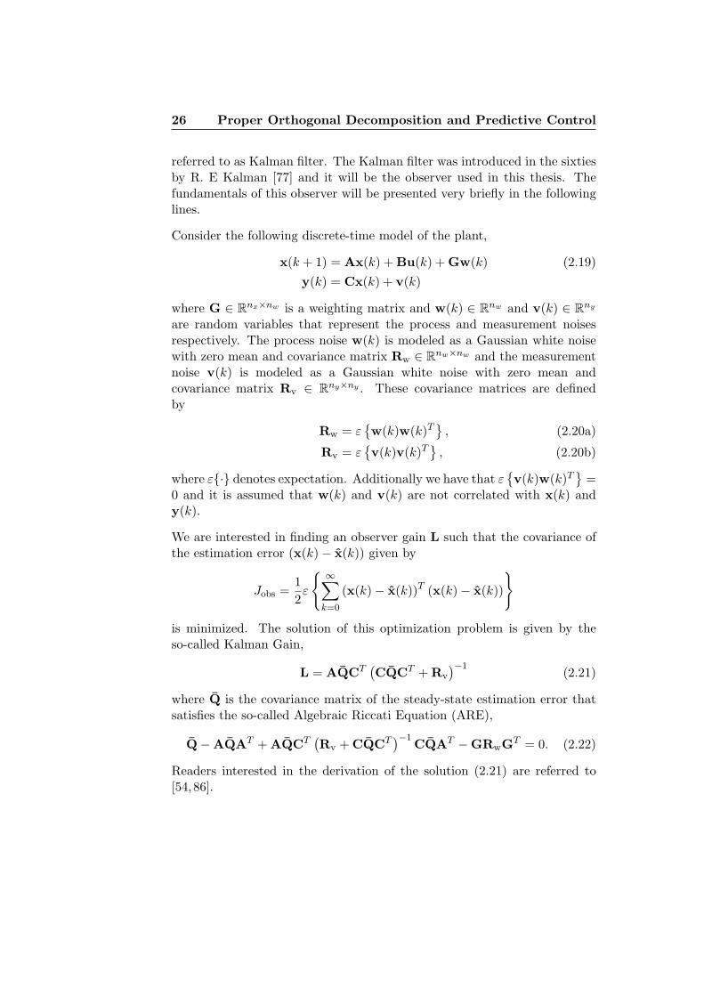
referred to as Kalman filter. The Kalman filter was introduced in the sixtiesby R. E Kalman [77] and it will be the observer used in this thesis. Thefundamentals of this observer will be presented very briefly in the followinglines.
Consider the following discrete-time model of the plant,
x(k + 1) = Ax(k) + Bu(k) + Gw(k) (2.19)y(k) = Cx(k) + v(k)
where G ∈ Rnx×nw is a weighting matrix and w(k) ∈ R
nw and v(k) ∈ Rny
are random variables that represent the process and measurement noisesrespectively. The process noise w(k) is modeled as a Gaussian white noisewith zero mean and covariance matrix Rw ∈ R
nw×nw and the measurementnoise v(k) is modeled as a Gaussian white noise with zero mean andcovariance matrix Rv ∈ R
ny×ny . These covariance matrices are definedby
Rw = ε{w(k)w(k)T
}, (2.20a)
Rv = ε{v(k)v(k)T
}, (2.20b)
where ε{·} denotes expectation. Additionally we have that ε{v(k)w(k)T
}=
0 and it is assumed that w(k) and v(k) are not correlated with x(k) andy(k).
We are interested in finding an observer gain L such that the covariance ofthe estimation error (x(k) − x(k)) given by
Jobs =12ε
{ ∞∑k=0
(x(k) − x(k))T (x(k) − x(k))
}
is minimized. The solution of this optimization problem is given by theso-called Kalman Gain,
L = AQCT(CQCT + Rv
)−1(2.21)
where Q is the covariance matrix of the steady-state estimation error thatsatisfies the so-called Algebraic Riccati Equation (ARE),
Q − AQAT + AQCT(Rv + CQCT
)−1CQAT − GRwGT = 0. (2.22)
Readers interested in the derivation of the solution (2.21) are referred to[54,86].
2.4 Example: Temperature control in a one–dimensional bar 27
Finally, we want to stress that for the control of high-dimensional systems,the MPC controller and the Kalman Filter in Figure 2.2 will be designedfrom the reduced order model of the process obtained by means of the PODand Galerkin projection techniques.
2.4 Example: Temperature control in a one–dimensional bar
For illustration purposes, in this section we present the application of PODand predictive control techniques to the control of the temperature profile ofa one-dimensional bar [2]. Initially an MPC controller without a disturbancemodel is designed. The control objective is to allow the bar to reach a desiredtemperature distribution in steady state as fast as possible, satisfying at thesame time the process constraints. Afterwards, an MPC with a disturbancemodel is implemented in order to reject the perturbations that affect thebar. Both MPCs are based on the reduced order model of the system foundby using POD and Galerkin projection.
2.4.1 Heat transfer in a one-dimensional bar
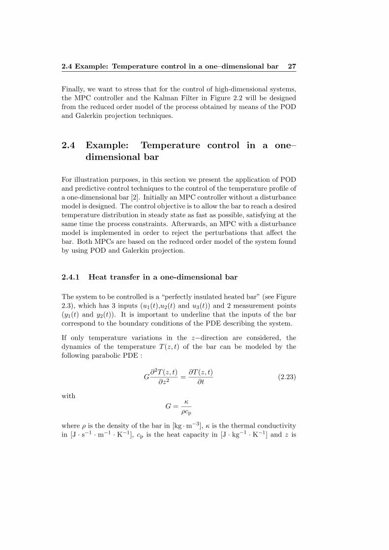
The system to be controlled is a “perfectly insulated heated bar” (see Figure2.3), which has 3 inputs (u1(t),u2(t) and u3(t)) and 2 measurement points(y1(t) and y2(t)). It is important to underline that the inputs of the barcorrespond to the boundary conditions of the PDE describing the system.
If only temperature variations in the z−direction are considered, thedynamics of the temperature T (z, t) of the bar can be modeled by thefollowing parabolic PDE :
G∂2T (z, t)
∂z2=
∂T (z, t)∂t
(2.23)
withG =
κ
ρcp
where ρ is the density of the bar in [kg ·m−3], κ is the thermal conductivityin [J · s−1 · m−1 · K−1], cp is the heat capacity in [J · kg−1 · K−1] and z is

28 Proper Orthogonal Decomposition and Predictive Control
1( )u t 2 ( )u t 3 ( )u t
1( )y t 2 ( )y t
L0z
Figure 2.3: Heated bar. The signals u1(t), u2(t) and u3(t) are the boundaryconditions at z = 0, z = L/2 and z = L. The measured outputs y1(t) andy2(t) are the temperatures of the bar at z = L/4 and z = 3L/4 respectively.
1( )u k 2 ( )u k 3 ( )u k
0z 1z 2z 3z Pz1Pz 1Pz Nz1Nz2Nz
z
Grid points
Figure 2.4: Spatial discretization of the bar.
the position in [m]. The initial and boundary conditions (Dirichlet type) of(2.23) are given by,
T (z, 0) = T0(z), (2.24a)
T (0, t) = u1(t), T (L/2, t) = u2(t), T (L, t) = u3(t). (2.24b)
The length of the bar is L = 0.1 m and the parameter G is equal to 10−5. Theinitial temperature distribution is set to T0(z) = 0◦C and the input signalsu1(t), u2(t) and u3(t) must be between 0◦C and 150◦C (input constraints).
2.4.2 Discretization
For design and simulation purposes, Equation (2.23) is discretized in space(see Figure 2.4) and time by means of the “Implicit Backward Euler method”(a finite difference method), which unlike the “Explicit Forward Eulermethod”, is unconditionally stable [155]. The stability condition of the

2.4 Example: Temperature control in a one–dimensional bar 29
explicit forward Euler algorithm turns out to be G ΔtΔz2 ≤ 1
2 . This impliesthat as we decrease the spatial interval Δz for better accuracy, we mustalso decrease the time step Δt at the cost of more computations in ordernot to lose the stability. In the backward Euler method, the second partialderivative with respect to z is replaced by a central difference approximation,and the time derivative by a backward difference approximation as follows:
G
(Ti+1(k) − 2Ti(k) + Ti−1(k)
Δz2
)=
Ti(k) − Ti(k − 1)Δt
(2.25)
for i = 1, 2, . . . , P − 1, P + 1, . . . , N − 1
for k = 1, 2, . . . , M
with
T0(k) = u1(k), TP (k) = u2(k), TN (k) = u3(k),
where N is the number of sections in which the bar is divided, Δz is thelength of each section, Δt is the sampling time, Ti(k) = T (zi, tk) is thetemperature in the grid point zi = iΔz at the time tk = kΔt, P is the gridpoint where u2(t) is located (z = L/2) and M is the number of time steps.
If we define T(k) ∈ RN−2 = [T1(k), . . . , TP−1(k), TP+1(k), . . . , TN−1(k)]T
as the vector containing the temperatures of the grid points zi,∀i =1, 2, . . . , P − 1, P + 1, . . . , N − 1 at each time step k, Equation (2.25) can becast into a recursive linear system of equations as follows:
AT(k + 1) = T(k) + Bu(k)
T(k + 1) = A−1T(k) + A−1Bu(k) (2.26)
where u(k) = [u1(k), u2(k), u3(k)]T is the vector of inputs, and A ∈R
(N−2)×(N−2) and B ∈ R(N−2)×3 are the matrices describing the system
defined as follows,
A =[
As 00 As
], B =
⎡⎣ r 0 · · · 0 0 0 0 · · · 0 0
0 0 · · · 0 r r 0 · · · 0 00 0 · · · 0 0 0 0 · · · 0 r
⎤⎦T
,

30 Proper Orthogonal Decomposition and Predictive Control
with
As ∈ R(P−1)×(P−1) =
⎡⎢⎢⎢⎢⎢⎢⎢⎣
1 + 2r −r 0 · · · 0
−r 1 + 2r. . . . . .
...
0 −r. . . −r 0
.... . . . . . 1 + 2r −r
0 · · · 0 −r 1 + 2r
⎤⎥⎥⎥⎥⎥⎥⎥⎦, r = G
Δt
Δz2.
In this example the sampling time is set to 1 s, and the spatial domain isdivided into N = 400 sections which means that Equation (2.26) has N − 2= 398 states. This large number of states makes the design of feedbackcontrollers for the bar difficult. Therefore, it is necessary to find a reducedorder model. Such a model is derived in the following subsection by usingPOD and Galerkin projection.
2.4.3 Model reduction using POD
For deriving a reduced order model of (2.26), the subsequent steps werefollowed:
1. Generation of the Snapshot Matrix. We have constructeda snapshot matrix Tsnap ∈ R
398×500 from the system responsewhen Pseudo Random Binary Noise Signals (PRBNS) were appliedsimultaneously to the inputs u1(k), u2(k), and u3(k) of the discretemodel of the bar (2.26),
Tsnap = [T(k = 1),T(k = 2), . . . ,T(k = 500)] . (2.27)
Along the simulations, a switching probability of 2% and an amplitudeof 100◦C were set to the PRBNS signals, and 500 samples werecollected using a sampling time of 1 s.
2. Derivation of the POD basis vectors. As it was explained inSection 2.2.1, the POD basis vectors are found by calculating the SVDof the snapshot matrix Tsnap,
Tsnap = ΦΣΨT
where Φ ∈ R398×398 and Ψ ∈ R
500×500 are unitary matrices, andΣ ∈ R
398×500 is a matrix containing the singular values of Tsnap in a

2.4 Example: Temperature control in a one–dimensional bar 31
0 10 20 30 40 5010
−16
10−14
10−12
10−10
10−8
10−6
10−4
10−2
100
n
1−
Pn
Figure 2.5: The logarithmic plot of 1 − Pn which is used to determine thetruncation degree of the POD basis vectors.
decreasing order on its main diagonal. The left singular vectors, thatis, the columns of the matrix Φ,
Φ = [ϕ1,ϕ2, . . . ,ϕ398]
are the POD basis vectors.
3. Selection of the most relevant POD basis vectors. The nmost relevant POD basis vectors are chosen using the energy criterionpresented in Section 2.2.1. The plot of 1 − Pn (see Equation (2.7))for the first 50 basis vectors is shown in Figure 2.5. In this case, weselected the first n = 10 POD basis vectors (they are shown in Figure2.6) based on their truncation degree 1− Pn = 2.454 · 10−5. Thus, the10th order approximation of T(k) is given by
Tn(k) =10∑
j=1
aj(k)ϕj = Φna(k) (2.28)
where Φn = [ϕ1,ϕ2, . . . ,ϕ10] and a(k) = [a1(k), a2(k), . . . , a10(k)]T .
4. Construction of the model for the first n=10 POD coeffi-cients. As it was explained in Section 2.2.2, the dynamic model for the

32 Proper Orthogonal Decomposition and Predictive Control
0 0.05 0.1−0.07
−0.05
−0.03
0 0.05 0.1−0.1
0.025
0.15
0 0.05 0.1−0.2
−0.075
0.05
0 0.05 0.1−0.1
0.025
0.15
0 0.05 0.1−0.2
−0.025
0.15
0 0.05 0.1−0.2
−0.025
0.15
0 0.05 0.1−0.25
−0.05
0.15
0 0.05 0.1−0.25
−0.075
0.1
0 0.05 0.1−0.2
0
0.2
0 0.05 0.1−0.2
0.025
0.25
ϕ1 ϕ2 ϕ3
ϕ4 ϕ5 ϕ6
ϕ7 ϕ8 ϕ9
ϕ10
z [m]
z [m]z [m]
Figure 2.6: Selected POD basis vectors.
POD coefficients can be derived by projecting (Galerkin projection)the model (2.26) on the space spanned by the selected POD basisvectors Φn = [ϕ1,ϕ2, . . . ,ϕ10]. If we replace T(k) by its nth orderapproximation Tn(k) = Φna(k) in Equation (2.26), and we apply theinner product criterion (Galerkin projection) to the resulting equation,we have that⟨
Φna(k + 1),ϕj
⟩=⟨A−1Φna(k) + A−1Bu(k),ϕj
⟩, (2.29)
∀j = 1, 2, . . . , n = 10.

2.4 Example: Temperature control in a one–dimensional bar 33
By evaluating the inner product in (2.29),
ΦTnΦna(k + 1) = ΦT
nA−1Φna(k) + ΦTnA−1Bu(k)
a(k + 1) = ΦTnA−1Φna(k) + ΦT
nA−1Bu(k) (2.30)
we obtain the model for the first n POD coefficients. The reducedorder model of the bar with only 10 states is then given by
a(k + 1) = Aa(k) + Bu(k) (2.31)Tn(k) = Φna(k)
where A ∈ R10×10 = ΦT
nA−1Φn and B ∈ R10×3 = ΦT
nA−1B.
For validating the reduced order model, constant inputs u1(k) = 0◦C,u2(k) = 100◦C and u3(k) = 50◦C were applied to the full order model andto the reduced order model, and afterwards their outputs were compared.Figure 2.7 shows the temperature profile of the bar at the time steps k = 1,k = 25, k = 50 and k = 250 for each model. It is really difficult to observedifferences between the responses of the models. Figure 2.8 presents the plotof the average of the absolute error which was calculated by means of thefollowing formula:
ET =1Ns
Ns∑k=1
|T(k) − Tn(k)|
where Ns = 250 is the number of simulation time steps. The maximum peakin Figure 2.8 is only 0.198◦C, which means that the reduced order modelwith only 10 states approximates very well the behavior of the full ordermodel (398 states).
2.4.4 MPC control scheme without a disturbance model
The control goal is to allow the bar to reach a desired temperaturedistribution in steady state as fast as possible. In addition, the controlactions must satisfy the input constraints of the process, that is, 0◦C ≤u1(k), u2(k), u3(k) ≤ 150◦C. In the top plot of Figure 2.10, the desired tem-perature profile Tref ∈ R
398 for the bar can be observed. This temperatureprofile corresponds to the steady state temperature distribution when thebar is heated from zero temperature by constant inputs u1(k) = 30◦C,u2(k) = 60◦C and u3(k) = 10◦C. The control of the temperature profile

34 Proper Orthogonal Decomposition and Predictive Control
0 0.05 0.1−20
0
20
40
60
80
100
0 0.05 0.1−20
0
20
40
60
80
100
0 0.05 0.10
20
40
60
80
100
0 0.05 0.10
20
40
60
80
100
Tem
per
atu
re[◦
C]
Tem
per
atu
re[◦
C]
Tem
per
atu
re[◦
C]
Tem
per
atu
re[◦
C] k = 1 k = 25
k = 50 k = 250
z [m]z [m]
z [m]z [m]
Figure 2.7: Temperature profile at different time steps. Solid line - Fullorder model (2.26). Dashed line - Reduced order model (2.31).
of the bar is achieved indirectly by controlling the POD coefficients. Thereferences (aref) of these POD coefficients can be calculated by
aref = ΦTnTref . (2.32)
For controlling the first n = 10 POD coefficients and consequently thetemperature profile of the bar, we initially implemented the MPC controlscheme shown in Figure 2.9. In this scheme the MPC controller uses thereduced order model given by (2.31) to predict the future behavior of theprocess. An observer, which in this case is a Kalman filter, is used forestimating the state of the reduced order model from the measurementsy(k) = [y1(k), y2(k)]T and the process inputs u(k) = [u1(k), u2(k), u3(k)]T .The observer equations are given by,
a(k + 1) = Aa(k) + Bu(k) + L (y(k) − y(k)) (2.33)
y(k) = CsTn(k) = CsΦna(k)

2.4 Example: Temperature control in a one–dimensional bar 35
0 0.02 0.04 0.06 0.08 0.10
0.02
0.04
0.06
0.08
0.1
0.12
0.14
0.16
0.18
0.2E
T[◦
C]
z [m]
Figure 2.8: Average of the absolute error between the full order model andthe reduced order model.
Full order Model of the Bar
KalmanFilter
MPCController
( )ku
( )ky
ˆ( )ka
ref ( )ka ( )kT
Temperature Profile
Measurement Points
Figure 2.9: MPC control scheme without a disturbance model.
where a(k) is the estimated vector of the POD coefficients, y(k) andTn(k) are the estimations of the output vector y(k) and the nth orderapproximation of the temperature profile Tn(k) respectively, L is theobserver gain (Kalman gain) and Cs is a selection matrix which selectsthe measured temperatures (y1(k) and y2(k)) from the vector Tn(k). TheKalman gain was calculated from the following covariance matrices: Rv =10−6 · I2, Rw = I10. Here, Rv is the covariance matrix of the measurementnoise (v(k)) and Rw is the covariance matrix of the process noise (w(k)).The diagonal of Rv contains the measured noise variance of each output
36 Proper Orthogonal Decomposition and Predictive Control
signal which are assumed to be uncorrelated. For this example thesevalues were assumed to be equal to 10−6. Physically, Rw tries to explainunknown disturbances, whether they are steps, white noise, or imperfectionsin the model of the plant. This parameter can be used to trade speed androbustness. In this case, Rw was chosen to be equal to the identity matrix.The simulations results confirmed that it was an appropriated choice forcalculating the observer gain.
The estimated state a(k) is used together with the reference vector aref
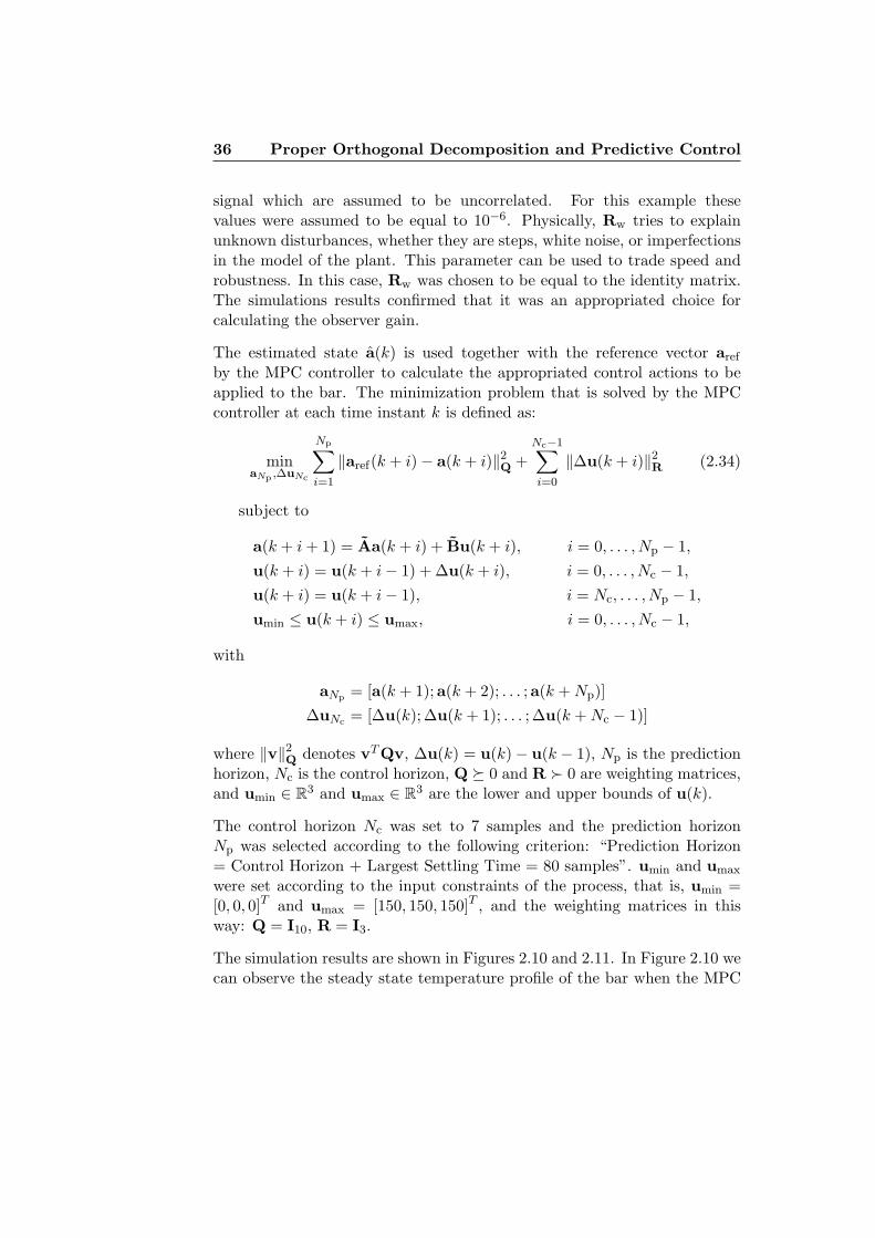
by the MPC controller to calculate the appropriated control actions to beapplied to the bar. The minimization problem that is solved by the MPCcontroller at each time instant k is defined as:
minaNp ,ΔuNc
Np∑i=1
‖aref(k + i) − a(k + i)‖2Q +
Nc−1∑i=0
‖Δu(k + i)‖2R (2.34)
subject to
a(k + i + 1) = Aa(k + i) + Bu(k + i), i = 0, . . . , Np − 1,
u(k + i) = u(k + i − 1) + Δu(k + i), i = 0, . . . , Nc − 1,
u(k + i) = u(k + i − 1), i = Nc, . . . , Np − 1,
umin ≤ u(k + i) ≤ umax, i = 0, . . . , Nc − 1,
with
aNp = [a(k + 1); a(k + 2); . . . ; a(k + Np)]ΔuNc = [Δu(k); Δu(k + 1); . . . ; Δu(k + Nc − 1)]
where ‖v‖2Q denotes vTQv, Δu(k) = u(k) − u(k − 1), Np is the prediction
horizon, Nc is the control horizon, Q � 0 and R 0 are weighting matrices,and umin ∈ R
3 and umax ∈ R3 are the lower and upper bounds of u(k).
The control horizon Nc was set to 7 samples and the prediction horizonNp was selected according to the following criterion: “Prediction Horizon= Control Horizon + Largest Settling Time = 80 samples”. umin and umax
were set according to the input constraints of the process, that is, umin =[0, 0, 0]T and umax = [150, 150, 150]T , and the weighting matrices in thisway: Q = I10, R = I3.
The simulation results are shown in Figures 2.10 and 2.11. In Figure 2.10 wecan observe the steady state temperature profile of the bar when the MPC
2.4 Example: Temperature control in a one–dimensional bar 37
0 0.02 0.04 0.06 0.08 0.10
20
40
60Temperature profile in steady state
0 0.02 0.04 0.06 0.08 0.10.02
0.03
0.04
0.05
0.06Absolute error
ReferenceClosed−loop
Tem
per
atu
re[◦
C]
Tem
per
atu
re[◦
C]
z [m]
z [m]
Figure 2.10: Steady-state temperature profile of the bar when the MPCcontroller (2.34) is used.
controller (2.34) is used. Also the absolute error between the reference andthe steady state response of the closed loop system is shown. The maximumdeviation in the temperature profile is only 0.055◦C. Figure 2.11 presentsthe evolution in time of the temperature at the measurement points and thecontrol actions of the MPC controller, which satisfy the input constraintsof the process. The closed-loop responses reach steady state faster thanthe open loop responses because the control system pushes the inputs tothe limits. In spite of the dramatic reduction of model order, on which thecontroller is based, the controller performs very well.
Now, we are going to suppose that the left edge of the bar is exposed to theambient temperature (20◦C) from a specific time instant. It implies thattemperature at the left edge would be given by the ambient temperatureplus u1(k). Figure 2.12 presents the steady state temperature profile of thebar in disturbed conditions with the MPC controller. It is clear that thebehavior of the control system in the presence of input disturbances is not

38 Proper Orthogonal Decomposition and Predictive Control
0 50 100 150 2000
10
20
30
40
50
0 50 100 150 2000
10
20
30
40
0 100 2000
26
52
78
104
130
0 100 20050
75
100
125
150
0 100 2000
20
40
60
80
y1(k
)-Tem
per
atu
re[◦
C]
y2(k
)-Tem
per
atu
re[◦
C]
u1(k
)-Tem
per
atu
re[◦
C]
u2(k
)-Tem
per
atu
re[◦
C]
u3(k
)-Tem
per
atu
re[◦
C]
samples - ksamples - ksamples - k
samples - ksamples - k
Figure 2.11: Temperature at the measurement points and control actions ofthe MPC controller (2.34). Solid line - Closed-loop response. Dashed line -Open loop response.
good. At the left edge of the bar there is a large temperature deviation of14.22◦C. This was an expected result, since the control scheme does notinclude a mechanism for rejecting such kind of disturbances. So, in order toovercome such limitation, an MPC controller with a disturbance model isdesigned and presented in the next subsection.
2.4.5 MPC control scheme with a disturbance model
The new MPC control scheme can be observed in Figure 2.13. Theformulation of the MPC controller with a disturbance model is given by
minaNp ,ΔuNc
Np∑i=1
‖aref(k + i) − a(k + i)‖2Q +
Nc−1∑i=0
‖Δu(k + i)‖2R (2.35a)
subject to
a(k + i + 1) = Aa(k + i) + Bu(k + i) + Fd(k + i), i = 0, . . . , Np − 1,

2.4 Example: Temperature control in a one–dimensional bar 39
d(k + i + 1) = d(k + i), i = 0, . . . , Np − 1,(2.35b)
u(k + i) = u(k + i − 1) + Δu(k + i), i = 0, . . . , Nc − 1,
u(k + i) = u(k + i − 1), i = Nc, . . . , Np − 1,
umin ≤ u(k + i) ≤ umax, i = 0, . . . , Nc − 1,
with
aNp = [a(k + 1); a(k + 2); . . . ; a(k + Np)]ΔuNc = [Δu(k); Δu(k + 1); . . . ; Δu(k + Nc − 1)]
where F is the disturbance model matrix, d(k) ∈ R is the disturbancesignal and Equation (2.35b) is the disturbance equation, which in this casecorresponds to a step. Since the disturbance d(k) and the state a(k) areunknown, they must be estimated by means of a new Kalman filter with thefollowing formulation:[
a(k + 1)d(k + 1)
]=[
A F0 1
] [a(k)d(k)
]+[
B0
]u(k)+ (2.36)
+[
La
Ld
](y(k) − y(k))
y(k) = CsTn(k) = CsΦna(k)
where a(k) is the estimated state, d(k) is the estimated disturbance vector,y(k) is the estimated output vector,
[LT
a ,LTd
]T is the Kalman gain and Cs
is a selection matrix which selects the measured temperatures (y1(k) andy2(k)) from the vector Tn(k).
The number of disturbance terms that can be estimated without losingobservability is equal to the number of sensors [114]. This means thatin this problem we might estimate at most 2 disturbance signals. In theMPC formulation (2.35) the disturbance model is defined by the matrix F.Since we are interested in rejecting the disturbance associated to the inputu1(k) (left edge of the bar), the matrix F is chosen in the following way:F = B(:, 1), where B(:, 1) denotes the first column of the matrix B.
The control and prediction horizon were set to 7 samples and 80 samplesrespectively, umin and umax were selected according to the input constraintsof the process and the weighting matrices in this way: Q = I10, R = I3.

40 Proper Orthogonal Decomposition and Predictive Control
0 0.02 0.04 0.06 0.08 0.10
20
40
60Temperature profile in steady state
0 0.02 0.04 0.06 0.08 0.10
5
10
15Absolute error
ReferenceClosed−loop
Tem
per
atu
re[◦
C]
Tem
per
atu
re[◦
C]
z [m]
z [m]
Figure 2.12: Steady-state temperature profile of the bar in disturbedconditions with the MPC controller (2.34).
Full order Model of the Bar
KalmanFilter
MPCController
( )ku
( )ky
ˆ( )ka
ref ( )ka ( )kT
Temperature Profile
Measurement Points
ˆ( )d k ( )d k
Figure 2.13: MPC control scheme with a disturbance model.
The simulation results of the MPC controller with an input disturbancemodel are shown in Figures 2.14 and 2.15. The left edge of the bar wasexposed to the ambient temperature at the time step k = 201. Figures2.14 and 2.15 show the evolution of the temperature profile before and afterthe disturbance respectively. The controller works very well and rejects

2.4 Example: Temperature control in a one–dimensional bar 41
0 0.05 0.10
50
100
150
0 0.05 0.10
20
40
60
80
0 0.05 0.10
20
40
60
80
0 0.05 0.10
20
40
60
Tem
per
atu
re[◦
C]
Tem
per
atu
re[◦
C]
Tem
per
atu
re[◦
C]
Tem
per
atu
re[◦
C] k = 1 k = 20
k = 40 k = 200
z [m]z [m]
z [m]z [m]
Figure 2.14: Evolution of the temperature profile before the disturbance(MPC with a disturbance model). Solid line - Closed-loop response. Dashedline - Reference.
0 0.05 0.10
20
40
60
0 0.05 0.110
20
30
40
50
60
0 0.05 0.110
20
30
40
50
60
0 0.05 0.110
20
30
40
50
60
Tem
per
atu
re[◦
C]
Tem
per
atu
re[◦
C]
Tem
per
atu
re[◦
C]
Tem
per
atu
re[◦
C] k = 201 k = 210
k = 220 k = 400
z [m]z [m]
z [m]z [m]
Figure 2.15: Evolution of the temperature profile after the disturbance(MPC with a disturbance model). Solid line - Closed-loop response. Dashedline - Reference.

42 Proper Orthogonal Decomposition and Predictive Control
0 100 200 300 4000
10
20
30
40
50
0 100 200 300 4000
10
20
30
40
0 200 4000
26
52
78
104
130
0 200 40050
75
100
125
150
0 200 4000
20
40
60
80
y1(k
)-Tem
per
atu
re[◦
C]
y2(k
)-Tem
per
atu
re[◦
C]
u1(k
)-Tem
per
atu
re[◦
C]
u2(k
)-Tem
per
atu
re[◦
C]
u3(k
)-Tem
per
atu
re[◦
C]
samples - ksamples - ksamples - k
samples - ksamples - k
d(k)
d(k)d(k) d(k)
d(k)
Figure 2.16: Temperature at the measurement points and control actions ofthe MPC controller (2.35) before and after the disturbance.
the perturbation quickly. In steady state, the maximum deviation in thetemperature profile is only 0.21◦C which is practically negligible. Thecontrol actions of the MPC Controller with a disturbance model as well asthe evolution of the temperature at the measurement points can be observedin Figure 2.16. The control actions are all the time within the limits.
2.5 Conclusions
In this chapter we have presented the basics of Proper Orthogonal De-composition (POD) and Galerkin projection, and we have shown howthese two techniques can be used for deriving reduced order models ofhigh-dimensional systems, typically obtained after discretizing in space thePDEs that model many processes. Furthermore we have presented thefundamentals of Model Predictive Control (MPC) and we have reviewedvery briefly the basic ideas behind the Kalman filter. In the last section of

2.5 Conclusions 43
this chapter, we have included a very detailed example where the mentionedtechniques have been used to control the temperature profile of a one-dimensional bar. In the example, a big model order reduction is achievedthanks to the POD technique that makes possible the control design.Initially, an MPC controller without a disturbance model was developed forcontrolling the temperature distribution when no input disturbances wereapplied to the bar. Its performance was very good in spite of the dramaticreduction of model order on which the controller is based. Afterwards, anMPC controller with a disturbance model was designed in order to rejectthe kind of disturbances that affect the system. This controller worked verywell and rejected the perturbations quickly.

44 Proper Orthogonal Decomposition and Predictive Control

Chapter 3
Control of a Non-isothermalTubular Reactor
3.1 Introduction
In this chapter the control of a non-isothermal tubular chemical reactoris addressed using POD and predictive control techniques. The controlgoal is to maintain the reactor at a desired operating condition in spiteof disturbances in the feed flow, while keeping the maximum temperatureinside the reactor low enough to avoid the formation of undesirablebyproducts. The operating condition of the reactor is determined by meansof an optimization algorithm which provides the optimal temperature andconcentration profiles for the process [3]. This algorithm, which takes intoaccount the input and state constraints of the system, is described in detailin this chapter. For controlling the reactor, we propose two MPC controlschemes: an MPC where its formulation is in terms of the POD coefficients(similar to the formulation of the MPCs used to control the bar in Section2.4) [3] and an MPC whose formulation is in terms of physical variables (thetemperature of some selected points and the concentration at the reactoroutlet) [4]. Unlike the first MPC controller, the second one incorporates thetemperature constraint of the reactor in some selected points of the spatialdomain. This MPC handles this constraint as a soft-constraint using a slackvariable approach with l∞-norm and time-dependent weights to deal withthe infeasibilities that can emerge [68,69].
45

46 Control of a Non-isothermal Tubular Reactor
Both MPC controllers are based on a linear model derived by meansof the POD and Galerkin projection techniques, which reduce the high-dimensionality of the discretized system used to approximate the linearPDEs that model the reactor around the operating profiles. In this chapterseveral tests are carried out in order to evaluate the performance of the MPCcontrollers.
This chapter is organized as follows. In Section 3.2 we present a descriptionof the tubular reactor that is used along this dissertation. We provideboth the nonlinear and linear mathematical models of the system, andadditionally we introduce the optimization algorithm for deriving theoperating profiles of the reactor. Section 3.3 shows the derivation of thereduced order model of the process using POD and Galerkin projection. InSection 3.4 the design and implementation of the MPC control schemes isdescribed. Section 3.5 presents some simulation results, and finally Section3.6 summarizes the main conclusions.
3.2 Tubular chemical reactor
A chemical reactor is basically a vessel where chemical reactions take place.A reactor is usually the heart of an overall chemical or biochemical process.In order to model the behavior of most chemical reactors there are threemain basic models that are commonly used, namely, the batch reactormodel (batch), the Continuous Stirred-Tank Reactor (CSTR) model andthe Plug Flow Reactor (PFR) model [122]. Plug flow reactors are alsocalled Continuous Tubular Reactors (CTRs) or simply tubular reactors andnowadays are widespread in chemical industry. In [95], a tubular chemicalreactor is defined and described as a tube in which chemical reactions takeplace during the continuous axial transport of the reaction mixture from theinlet towards the outlet. Typically, they are operated under time-invariantor steady-state conditions which leads to the production of large amounts ofproducts with a constant and high quality. One big advantage of this kindof reactors is the possibility of large-scale and low cost production relatedto their continuous operation since there are no down times as there are inbatch processes. Furthermore, they are suitable for advanced, automatedprocess control and optimization techniques, and they deliver constant andhigh product quality due to the tight monitoring and control of the reactionenvironment. However, they have some disadvantages, the investment costs

3.2 Tubular chemical reactor 47
are larger than in the other kinds of reactors and they are not suitable toproduce a variety of products in small amounts since the switching betweenproducts can lead to a considerable amount of off-spec production [95].
For the sake of the generality of the results and conceptual contributions,in this dissertation we will focus our attention on an elementary reactionin an ideal plug-flow reactor model, instead of reactions in specific complexindustrial reactors. In the following subsection we will describe in detail thetype of tubular reactor for which we will design and implement POD-basedMPC control strategies.
3.2.1 Plug flow reactor model
The system to be controlled is a non-isothermal tubular reactor where asingle, first order, irreversible, exothermic reaction takes place (A → B).The reactor is surrounded by 3 cooling/heating jackets as it is shownin Figure 3.1. The temperature of the jackets fluids (TJ1, TJ2 and TJ3)can be manipulated independently in order to control the concentrationand temperature profiles in the reactor. It is assumed that the fluid ormixture flows as a plug through the reactor body in the axial direction.In this dynamic only three phenomena are taken into account, namely,convection (macroscopic movement of the fluid inside the reactor), reaction(transformation of the chemical species present in the reactor, while releasingheat at the same time) and heat transfer (between the reactor and itsjackets). In this study we are not considering the diffusion/dispersionphenomena and we are neglecting the heat transfer effects between thejackets fluids and the reactor wall. Under the previous assumptions, themathematical model of the tubular chemical reactor consists of the followingcoupled nonlinear PDEs:
∂C
∂t= −v
∂C
∂z− k0Ce−
ERT (3.1a)
∂T
∂t= −v
∂T
∂z+ GrCe−
ERT + Hr(Tw − T ) (3.1b)
Gr = −ΔHk0
ρCp, Hr =
4h
2rsρCp,
with the following boundary conditions:
C = Cin at z = 0 and T = Tin at z = 0.

48 Control of a Non-isothermal Tubular Reactor
L z
J1T
A B
J2T J3T
in in,C T
reactant
,C T
AreactantA
productB
aZ bZ0
1s 2s 3s
Figure 3.1: Tubular chemical reactor with 3 cooling/heating jackets.
Here C(z, t) is the reactant concentration in [mol/l], T (z, t) is the reactanttemperature in [K], v is the fluid superficial velocity in [m/s], ΔH is theheat of the reaction in [cal/mol] (ΔH < 0 for an exothermic reaction),ρ and Cp are the density in [kg/l] and the specific heat in [cal/kg/K] ofthe mix respectively, k0 is the kinetic constant in [1/s], E is the activationenergy in [cal/mol], R is the ideal gas constant in [cal/mol/K], h is the heattransfer coefficient in [cal/s/m2/K], rs is the reactor radius in [m], L is thereactor length in [m], Cin and Tin are the concentration in [mol/l] and thetemperature in [K] of the feed flow, z is the axial coordinate in [m], t isthe time in [s] and Tw(z, t) is the reactor wall temperature in [K] defined asfollows (see Figure 3.1),
Tw =
⎧⎨⎩
TJ1, 0 ≤ z < Za
TJ2, Za ≤ z < Zb
TJ3, Zb ≤ z ≤ L.
The parameters values of the reactor model are taken from [138] which wereinspired by the values given in [53]. These values are presented in Table3.1. Additionally, in Equation (3.1) the following assumptions have beenmade: perfect radial mixing (the reactor diameter is assumed to be smallenough such that radial and angular variations are negligible), a constantheat transfer between the jacket and the reactor, a constant volume of thefluid in the reactor, a constant density and heat capacity of the reactingfluid, a constant velocity, and a constant heat of reaction. In Equation(3.1) only the temperature dependence of the reaction rate is incorporatedthrough the Arrhenius law (kr = k0e
−E/(RT ), where kr is the reactionrate constant). This is not the case for the other properties where thetemperature dependence is neglected. As it is stated in [95], in spite ofthe conceptual and highly simplified character of model (3.1), this modelcan provide valuable insights for tubular reactors in practice, for example,

3.2 Tubular chemical reactor 49
Table 3.1: Values of the reactor parameters
Parameter Valuev 0.1 m·s−1
L 1 mk0 106 s−1
E 11250 cal·mol−1
R 1.986 cal·mol−1·K−1
Cin 0.02 mol·l−1
Tin 340 KGr 4.25 · 109 l·K·mol−1·s−1
Hr 0.2 s−1
in the production of low density polyethylene (LDPE) [30], or in oxidationprocesses in an environment with an excess of oxygen [52].
The temperature of the jacket sections TJ1, TJ2 and TJ3 must be between280 K and 400 K. In addition, the temperature inside the reactor must bebelow 400 K in order to avoid the formation of side products. The kindof disturbances that affects the reactor are principally the variations in thetemperature and concentration of the feed flow. Typically, such variationsare in the range of ±10 K for the temperature and ±5% of the nominalvalue for the concentration. In this system, only the temperature of thefeed flow is measured directly. In addition, the reactor has a temperaturesensor at the output and 3 temperature sensors (s1, s2 and s3) distributedin its interior as shown in Figure 3.1.
3.2.2 Operating profiles
The operating profiles (steady-state concentration and temperature profiles)of the reactor are derived by means of an optimization algorithm, whichminimizes a cost function subject to the steady-state equations of the reactordescribed by (3.1), and the input and state constraints defined previously.The steady-state model of the reactor is given by the following OrdinaryDifferential Equations (ODEs):
dC
dz= −k0
vCe−
ERT (3.2)
dT
dz=
Gr
vCe−
ERT +
Hr
v(Tw − T )

50 Control of a Non-isothermal Tubular Reactor
with T = Tin at z = 0 and C = Cin at z = 0, and the discrete version of(3.2) can be found by replacing the spatial derivatives by forward differenceapproximations as follows:
Ci+1 = Ci − k0Δz
vCie
−ERTf Ti (3.3)
Ti+1 = Ti
(1 − HrΔz
v
)+(
GrΔzCf
vTf
)Cie
−ERTf Ti +
(HrΔz
v
)Tw,i
for i = 1, 2, . . . , N = 300,
with
Tw,i =
⎧⎨⎩
TJ1 = TJ1/Tf , ∀i = 1, . . . , za
TJ2 = TJ2/Tf , ∀i = za + 1, . . . , zb
TJ3 = TJ3/Tf , ∀i = zb + 1, . . . , N
T0 =Tin
Tf
C0 =Cin
Cf
where N is the number of sections in which the reactor is divided, za andzb are the reactor sections defining the ending of the first and second jacketrespectively, Tf and Cf are normalization factors, Ci = Ci/Cf and Ti = Ti/Tf
are the normalized concentration and temperature of the ith section of thereactor, Tw,i = Tw,i/Tf is the normalized reactor wall temperature of the ithsection, and Δz is the length of each section. The variables are normalizedin order to avoid possible numerical problems. The optimization problemthat is solved for deriving the operating profiles is defined as:
minTJ1,TJ2,TJ3
w(Cr − CN )2 + (1 − w)1N
N∑i=1
(Tr,i − Ti
)2 (3.4)
subject to
steady − state model given by (3.3)TJmin
Tf≤ TJ1, TJ2, TJ3 ≤ TJmax
Tf
Ti ≤ Tmax
Tf, for i = 1, 2, . . . , N = 300,
where Cr is the normalized desired concentration at the reactor output, Tr,i
is the normalized desired temperature inside the reactor of the ith section,
3.2 Tubular chemical reactor 51
CN is the normalized concentration at the reactor output, w is a trade-offparameter, TJmin and TJmax are the limits of the jackets temperatures, andTmax is the maximum allowed temperature inside the tubular reactor.
The first term of the cost function corresponds to the squared error ofthe normalized concentration at the reactor output (terminal cost), andthe second term is related to the mean squared error of the normalizedtemperature along the reactor (integral cost). In this problem Cr was setto 0, and Tr,i was selected equal to the normalized temperature of thefeed flow (Tin = Tin/Tf) for i = 1, 2, . . . , N . The trade-off parameter wcan take values from 0 to 1. When w goes to 1, the reduction of thereactant concentration at the reactor output becomes more important thanthe temperature deviations. On the other hand when w goes to 0, thetemperature deviations become more important than the concentration atthe reactor output and the risk of the formation of hot spots is reduced.
In order to solve the optimization problem described by (3.4) the followingalgorithm (a sort of Sequential Quadratic Programming - SQP) is proposed:
1. Choose the initial values of the jackets temperatures T∗J =
[T ∗
J1, T∗J2, T
∗J3
]Tin such a way that the constraints are satisfied.
2. Using T∗J, simulate (3.3) in order to obtain the temperature (T∗ ∈ R
N )and concentration (C∗ ∈ R
N ) profiles of the reactor in steady state.
3. Linearize the nonlinear model given by (3.3) around T∗,C∗, and T∗J
by means of the Taylor series. The resulting linear model would havethe following structure:[
CΔi+1
TΔi+1
]= Ass(i)
[CΔ
i
TΔi
]+ BssT
Δw,i (3.5)[
Ci
Ti
]=[
CΔi
TΔi
]+[
C∗i
T ∗i
]
for i = 1, 2, . . . , N,
with
Ass(i) =
⎡⎢⎣ 1 − k0Δz
v e− E
RT∗i −k0TfEΔz
vCfRC∗
i
T ∗i
2 e− E
RT∗i
CfGrΔzvTf
e− E
RT∗i 1 − HrΔz
v + GrEΔzvR
C∗i
T ∗i
2 e− E
RT∗i
⎤⎥⎦ ,
52 Control of a Non-isothermal Tubular Reactor
Bss =[
0HrΔz
v
],
where Ass(i) and Bss are the matrices describing the system dy-namics, C∗
i , T ∗i and T ∗
w,i are the normalized operating points of theconcentration, temperature and reactor wall temperature of the ithsection, CΔ
i , TΔi and TΔ
w,i are the normalized deviation variables of theconcentration, temperature and reactor wall temperature respectively.
4. Solve the following Quadratic Problem (QP):
minTΔJ1,TΔ
J2,TΔJ3
w(Cr − CN )2 + (1 − w)1N
N∑i=1
(Tr,i − Ti
)2subject to
steady − state linear model given by (3.5)TJmin
Tf≤ TJ1, TJ2, TJ3 ≤ TJmax
Tf
−TΔmaxJ
Tf≤ TΔ
J1, TΔJ2, T
ΔJ3 ≤ TΔmax
J
Tf
Ti ≤ Tmax
Tf, for i = 1, 2, . . . , N = 300,
where TΔJ1, T
ΔJ2, T
ΔJ3 are the normalized deviation variables of the jackets
temperatures, and TΔmaxJ is a “local input constraint” which limits the
range of the jackets temperatures in such a way that the linear model(3.5) is still a good approximation of the nonlinear model (3.3). If thisis not the case, then we would have convergence problems.
5. Calculate the new jackets temperatures TopJ ∈ R
3 as follows:
TopJ = TΔ,op
J + T∗J
where TΔ,opJ =
[TΔ,op
J1 , TΔ,opJ2 , TΔ,op
J3
]Tis the solution of the QP
problem stated in the previous step.
6. Using TopJ , simulate (3.3) in order to obtain the new temperature
(Top ∈ RN ) and concentration (Cop ∈ R
N ) profiles of the reactor insteady state.

3.2 Tubular chemical reactor 53
7. If max(∣∣Top
J − T∗J
∣∣) ≤ Tol then stop, else make T∗J = Top
J , C∗ = Cop,T∗ = Top and go to step 3.
The proposed algorithm was executed with the following parameters : N =300, Tf = 340 K, Cf = 0.02 mole/l, Δz = 1/300 m, TJmin = 280 K, TJmax =400 K, Tmax = 390 K, Tol = 10−4, w = 0.3 and TΔmax
J = 20 K.
The maximum allowed temperature (Tmax) inside the reactor was chosen10 degrees below the actual limit (400 K) in order to give to the feedbackcontroller enough room of maneuverability. The trade-off coefficient w wasfound by trial and error and the local input constraint TΔmax
J was selectedin such a way that the differences between the nonlinear and linear modelare small.
The algorithm was executed using different initial conditions and some ofthe results obtained are presented in Table 3.2. Along the experiments,three local minima were found, however it does not mean that these arethe only ones. Figures 3.2, 3.3 and 3.4 show the reactor profiles associatedto these local minima. This result was expected due to the non-convexnature of the optimization problem. These local minima might be unifiedby modifying the cost function, for instance, by adding a term that penalizesthe temperature deviation at the reactor output.
The selection of the optimal temperature and concentration profiles wasdone by checking the value of the cost function and the deviation of thetemperature at the reactor output with respect to the temperature of thefeed flow. In many practical situations, a large deviation is undesirable sinceit increases the heat loss [137].
From the three local minima, the second one (TJ1 = 374.6 K, TJ2 = 310.1 Kand TJ3 = 325.2 K) was chosen since it has the smallest cost function valueand a small temperature deviation at the reactor output. The optimalconcentration and temperature profiles can be observed in Figure 3.4. Theconcentration at the reactor output is 1.5737 ·10−3 mol/l which is 12.7 timessmaller than the concentration of the feed flow (0.02 mol/l). In addition,the temperature of the hot spot is 390 K.
3.2.3 Linear model
The linear model of the tubular chemical reactor is obtained by linearizing(3.1) around the jackets temperatures and the operating profiles presented

54 Control of a Non-isothermal Tubular Reactor
0 0.2 0.4 0.6 0.8 1320
340
360
380
400
0 0.2 0.4 0.6 0.8 10
0.005
0.01
0.015
0.02
390 K
Tem
per
atu
re[K
]C
once
ntr
ati
on
[mol/
l]
Length z [m]
Length z [m]
Figure 3.2: Steady-state concentration and temperature profiles when TJ1 =359.6 K, TJ2 = 348.5 K and TJ3 = 291.5 K.
0 0.2 0.4 0.6 0.8 1320
340
360
380
400
0 0.2 0.4 0.6 0.8 10
0.005
0.01
0.015
0.02
390 K
Tem
per
atu
re[K
]C
once
ntr
ati
on
[mol/
l]
Length z [m]
Length z [m]
Figure 3.3: Steady-state concentration and temperature profiles when TJ1 =340.7 K, TJ2 = 355.1 K and TJ3 = 365.7 K.

3.2 Tubular chemical reactor 55
Table 3.2: Some results obtained with the optimization algorithm
Initial Jackets Final JacketsCost
Cin/CNNo.
Temperatures TemperaturesFunction Iter a
TJ1 TJ2 TJ3 TJ1 TJ2 TJ3
- First Minimum - (see Figure 3.2 )
300 300 300359.6 348.5 291.5 8.356 · 10−3 12.6
66350 350 350 73280 400 280 91
- Second Minimum - (see Figure 3.4)
350 280 350374.6 310.1 325.2 8.337 · 10−3 12.7
38370 290 370 39
- Third Minimum - (see Figure 3.3)
280 280 400340.7 355.1 365.7 8.416 · 10−3 12.7
29380 340 400 24
aNumber of iterations
0 0.2 0.4 0.6 0.8 1320
340
360
380
400
0 0.2 0.4 0.6 0.8 10
0.005
0.01
0.015
0.02
390 K
Tem
per
atu
re[K
]C
once
ntr
ati
on
[mol/
l]
Length z [m]
Length z [m]
Figure 3.4: Selected operating profiles. Steady-state concentration andtemperature profiles when TJ1 = 374.6 K, TJ2 = 310.1 K and TJ3 = 325.2 K.

56 Control of a Non-isothermal Tubular Reactor
in Figure 3.4. This linear model is given by,
∂CΔ
∂t= −v
∂CΔ
∂z− αA(z)CΔ − αB(z)TΔ (3.6)
∂TΔ
∂t= −v
∂TΔ
∂z− αC(z)CΔ − αD(z)TΔ + HrT
Δw
with
αA(z) = k0e− E
RT∗
αB(z) = k0C∗ E
RT ∗2 e−E
RT∗
αC(z) = −Gre− E
RT∗
αD(z) = −GrC∗ E
RT ∗2 e−E
RT∗ + Hr
and with these boundary conditions
CΔ = Cin − C∗in, TΔ = Tin − T ∗
in at z = 0.
Here C∗, T ∗ and T ∗w are the steady state profiles (operating profiles) of the
concentration, temperature and reactor wall temperature respectively, C∗in
and T ∗in are the concentration and temperature in steady state of the feed
flow, CΔ = C−C∗, TΔ = T −T ∗ and TΔw = Tw−T ∗
w are the deviations fromsteady state of the concentration, temperature and reactor wall temperature.
In order to reduce the infinite dimensionality of (3.6), the partial derivativeswith respect to space are replaced by backward difference approximationsleading to the following system of ODEs:
dCΔi
dt= − v
Δz
(CΔ
i − CΔi−1
)− αA,iCΔi − αB,i
Tf
CfTΔ
i (3.7)
dTΔi
dt= − v
Δz
(TΔ
i − TΔi−1
)− αC,iCf
TfCΔ
i − αD,iTΔi + HrT
Δw,i
for i = 1, 2, . . . , N,
withCΔ
0 = CΔin , TΔ
0 = TΔin ,
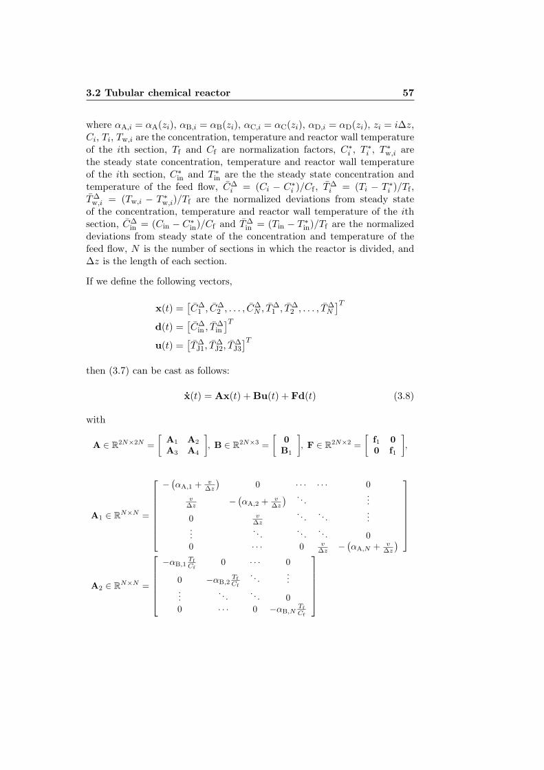
3.2 Tubular chemical reactor 57
where αA,i = αA(zi), αB,i = αB(zi), αC,i = αC(zi), αD,i = αD(zi), zi = iΔz,Ci, Ti, Tw,i are the concentration, temperature and reactor wall temperatureof the ith section, Tf and Cf are normalization factors, C∗
i , T ∗i , T ∗
w,i arethe steady state concentration, temperature and reactor wall temperatureof the ith section, C∗
in and T ∗in are the the steady state concentration and
temperature of the feed flow, CΔi = (Ci − C∗
i )/Cf , TΔi = (Ti − T ∗
i )/Tf ,TΔ
w,i = (Tw,i − T ∗w,i)/Tf are the normalized deviations from steady state
of the concentration, temperature and reactor wall temperature of the ithsection, CΔ
in = (Cin − C∗in)/Cf and TΔ
in = (Tin − T ∗in)/Tf are the normalized
deviations from steady state of the concentration and temperature of thefeed flow, N is the number of sections in which the reactor is divided, andΔz is the length of each section.
If we define the following vectors,
x(t) =[CΔ
1 , CΔ2 , . . . , CΔ
N , TΔ1 , TΔ
2 , . . . , TΔN
]Td(t) =
[CΔ
in , TΔin
]Tu(t) =
[TΔ
J1, TΔJ2, T
ΔJ3
]Tthen (3.7) can be cast as follows:
x(t) = Ax(t) + Bu(t) + Fd(t) (3.8)
with
A ∈ R2N×2N =
[A1 A2
A3 A4
], B ∈ R
2N×3 =[
0B1
], F ∈ R
2N×2 =[
f1 00 f1
],
A1 ∈ RN×N =
⎡⎢⎢⎢⎢⎢⎢⎢⎣
− (αA,1 + vΔz
)0 · · · · · · 0
vΔz − (αA,2 + v
Δz
) . . ....
0 vΔz
. . . . . ....
.... . . . . . . . . 0
0 · · · 0 vΔz − (αA,N + v
Δz
)
⎤⎥⎥⎥⎥⎥⎥⎥⎦
A2 ∈ RN×N =
⎡⎢⎢⎢⎢⎢⎣
−αB,1TfCf
0 · · · 0
0 −αB,2TfCf
. . ....
.... . . . . . 0
0 · · · 0 −αB,NTfCf
⎤⎥⎥⎥⎥⎥⎦

58 Control of a Non-isothermal Tubular Reactor
A3 ∈ RN×N =
⎡⎢⎢⎢⎢⎢⎣
−αC,1CfTf
0 · · · 0
0 −αC,2CfTf
. . ....
.... . . . . . 0
0 · · · 0 −αC,NCfTf
⎤⎥⎥⎥⎥⎥⎦
A4 ∈ RN×N =
⎡⎢⎢⎢⎢⎢⎢⎢⎣
− (αD,1 + vΔz
)0 · · · · · · 0
vΔz − (αD,2 + v
Δz
) . . ....
0 vΔz
. . . . . ....
.... . . . . . . . . 0
0 · · · 0 vΔz − (αD,N + v
Δz
)
⎤⎥⎥⎥⎥⎥⎥⎥⎦
B1 ∈ RN×3 =
⎡⎣ Hr · · · Hr 0 · · · 0 0 · · · 0
0 · · · 0 Hr · · · Hr 0 · · · 00 · · · 0 0 · · · 0 Hr · · · Hr
⎤⎦T
f1 ∈ RN =
[v
Δz 0 · · · 0]T
where T ∗J1, T ∗
J2, T ∗J3, are the steady state jacket temperatures, TΔ
J1 =(TJ1 − T ∗
J1) /Tf , TΔJ2 = (TJ2 − T ∗
J2) /Tf and TΔJ3 = (TJ3 − T ∗
J3) /Tf are thenormalized deviations of the jacket temperatures, A, B and F are thematrices describing the system, x(t) ∈ R
2N is the state vector, u(t) ∈ R3 is
the vector of the inputs and d(t) ∈ R2 is the vector of the disturbances.
Since the spatial domain of the reactor is divided into N = 300 sections, thenumber of states of (3.8) is equal to 600. Given that such large number ofstates makes the design and implementation of feedback controllers for thereactor difficult, in the next section a reduced order model will be derivedusing POD and Galerkin projection.
3.3 Model reduction using POD
In a similar fashion as it was done in Section 2.4.3, the reduced order modelof (3.8) is found by following the subsequent steps:
1. Generation of the Snapshot Matrix. We have created a snapshotmatrix Xsnap ∈ R
600×1500 from the system response when independentstep changes were made in the input u(t) and perturbation d(t) signals

3.3 Model reduction using POD 59
of the linear model (3.8),
Xsnap = [x(t = Δt),x(t = 2Δt), . . . ,x(t = 1500Δt)] . (3.9)
Along the simulations 1500 samples were collected using a samplingtime Δt of 0.05 s. The amplitude of the step changes was chosenin such a way as to produce changes of similar magnitude in thetemperature and concentration profiles. This avoids a possible biasin the resulting model.
2. Derivation of the POD basis vectors. The POD basis vectors areobtained by computing the SVD of the snapshot matrix Xsnap,
Xsnap = ΦΣΨT
where Φ ∈ R600×600 and Ψ ∈ R
1500×1500 are unitary matrices, andΣ ∈ � 600×1500 is a matrix that contains the singular values of Xsnap
in a decreasing order on its main diagonal. The left singular vectors,i.e., the columns of Φ,
Φ = [ϕ1,ϕ2, . . . ,ϕ600]
are the POD basis vectors.
3. Selection of the most relevant POD basis vectors. The nmost relevant POD basis vectors are chosen using the energy criterionpresented in Section 2.2.1. The plot of 1 − Pn (see Equation (2.7))for the first 160 basis vectors is shown in Figure 3.5. In this problem,we chose the first n = 20 POD basis vectors based on their truncationdegree 1−Pn = 3.3 ·10−4 (Pn = 0.9996). In Figures 3.6 and 3.7 we canobserve the basis vectors associated to the 20 largest singular vectors.Observe that the first half of each basis vector is associated to thenormalized deviations of the concentration profile whereas the secondhalf is related to the normalized deviations of the temperature profile.
The 20th order approximation of x(t) is given by the followingtruncated sequence:
xn(t) =20∑
j=1
aj(t)ϕj = Φna(t) (3.10)
where Φn = [ϕ1,ϕ2, . . . ,ϕ20] and a(t) = [a1(t), a2(t), . . . , a20(t)]T .
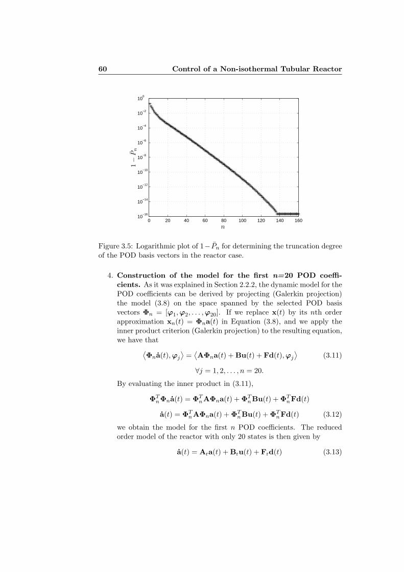
60 Control of a Non-isothermal Tubular Reactor
0 20 40 60 80 100 120 140 16010
−16
10−14
10−12
10−10
10−8
10−6
10−4
10−2
100
n
1−
Pn
Figure 3.5: Logarithmic plot of 1− Pn for determining the truncation degreeof the POD basis vectors in the reactor case.
4. Construction of the model for the first n=20 POD coeffi-cients. As it was explained in Section 2.2.2, the dynamic model for thePOD coefficients can be derived by projecting (Galerkin projection)the model (3.8) on the space spanned by the selected POD basisvectors Φn = [ϕ1,ϕ2, . . . ,ϕ20]. If we replace x(t) by its nth orderapproximation xn(t) = Φna(t) in Equation (3.8), and we apply theinner product criterion (Galerkin projection) to the resulting equation,we have that⟨
Φna(t),ϕj
⟩=⟨AΦna(t) + Bu(t) + Fd(t),ϕj
⟩(3.11)
∀j = 1, 2, . . . , n = 20.
By evaluating the inner product in (3.11),
ΦTnΦna(t) = ΦT
nAΦna(t) + ΦTnBu(t) + ΦT
nFd(t)
a(t) = ΦTnAΦna(t) + ΦT
nBu(t) + ΦTnFd(t) (3.12)
we obtain the model for the first n POD coefficients. The reducedorder model of the reactor with only 20 states is then given by
a(t) = Ara(t) + Bru(t) + Frd(t) (3.13)

3.3 Model reduction using POD 61
0 0.5 1−0.08
0
0.08
0 0.5 1 0 0.5 1−0.07
−0.005
0.06
0 0.5 1
0 0.5 1−0.1
−0.05
0
0.05
0 0.5 1 0 0.5 1−0.08
−0.03
0.02
0 0.5 1
0 0.5 1−0.1
−0.015
0.07
0 0.5 1 0 0.5 1−0.08
0
0.08
0 0.5 1−0.1
0
0.1
0 0.5 1 0 0.5 1−0.1
0
0.1
0 0.5 1
0 0.5 1−0.15
−0.025
0.1
0 0.5 1 0 0.5 1−0.1
0
0.1
0 0.5 1
0 0.5 1
temperature temperatureconcentration concentrationϕ1 ϕ2
ϕ3 ϕ4
ϕ5 ϕ6
ϕ7 ϕ8
ϕ9 ϕ10
z [m]z [m]z [m]z [m]
Figure 3.6: POD basis vectors : ϕ1,ϕ2, . . . ,ϕ10.
xn(t) = Φna(t)
where Ar = ΦTnAΦn, Br = ΦT
nB and Fr = ΦTnF. The initial condition
for a(t) reads as a(0) = 0.

62 Control of a Non-isothermal Tubular Reactor
0 0.5 1−0.1
−0.01
0.08
0 0.5 1 0 0.5 1−0.1
0
0.1
0 0.5 1
0 0.5 1−0.1
0.03
0.16
0 0.5 1 0 0.5 1−0.12
0
0.12
0 0.5 1
0 0.5 1−0.1
0
0.1
0 0.5 1 0 0.5 1−0.15
−0.015
0.12
0 0.5 1
0 0.5 1−0.13
0.005
0.14
0 0.5 1 0 0.5 1−0.14
−0.01
0.12
0 0.5 1
0 0.5 1−0.12
0.01
0.14
0 0.5 1 0 0.5 1−0.12
−0.01
0.1
0 0.5 1
temperature temperatureconcentration concentrationϕ11 ϕ12
ϕ13 ϕ14
ϕ15 ϕ16
ϕ17 ϕ18
ϕ19 ϕ20
z [m]z [m]z [m]z [m]
Figure 3.7: POD basis vectors : ϕ11,ϕ12, . . . ,ϕ20.
For validating the reduced order model of the reactor, we applied constantinput signals TΔ
J1(t) = 0.125 (TΔJ1(t) = 10 K), TΔ
J2(t) = −0.25 (TΔJ2(t) = −20
K) and TΔJ3(t) = 0.25 (TΔ
J3(t) = 20 K) and constant perturbation signalsCΔ
in (t) = 0.05 (CΔin (t) = 10−3 mol/l) and TΔ
in (t) = 0.0625 (TΔin (t) = 5 K)
to both the full order model (3.8) and the reduced order model (3.13),and afterwards we compared their responses. Figures 3.8 and 3.9 show the

3.3 Model reduction using POD 63
0 0.5 1−5
0
5
10
0 0.5 1−5
0
5
10
15x 10
−4
0 0.5 1−20
0
20
40
0 0.5 1−4
−2
0
2x 10
−3
Tem
per
atu
re[K
]
Tem
per
atu
re[K
]
Conce
ntr
ati
on
[mol/
l]
Conce
ntr
ati
on
[mol/
l]
z [m]
z [m]
z [m]
z [m]
Profiles at t = 1 s Profiles at t = 4 s
Figure 3.8: Temperature and concentration deviation profiles at t = 1 s andt = 4 s. Solid line - Full order model. Dashed line - Reduced order model.
0 0.5 1−10
0
10
20
30
0 0.5 1−6
−4
−2
0
2x 10
−3
0 0.5 1−10
0
10
20
30
0 0.5 1−6
−4
−2
0
2x 10
−3
Tem
per
atu
re[K
]
Tem
per
atu
re[K
]
Conce
ntr
ati
on
[mol/
l]
Conce
ntr
ati
on
[mol/
l]
z [m]
z [m]
z [m]
z [m]
Profiles at t = 8 s Profiles at t = 15 s
Figure 3.9: Temperature and concentration deviation profiles at t = 8 s andt = 15 s. Solid line - Full order model. Dashed line - Reduced order model.

64 Control of a Non-isothermal Tubular Reactor
0 0.2 0.4 0.6 0.8 10.1
0.2
0.3
0.4
0.5
0 0.2 0.4 0.6 0.8 12
4
6
8
10x 10
−5
z [m]
z [m]
ET
[K]
EC
[mol/
l]
Figure 3.10: Average of the absolute error between the full order model (3.8)and the reduced order model (3.13).
temperature and concentration deviation profiles of the reactor at differenttime instants for each model. During the first seconds we can see somedifferences between the models, but as the simulation advances, thesedifferences become negligible and really difficult to observe. In order tomeasure the quality of the reduced order model the averages of the absoluteerror for the temperature (ET) and concentration (EC) were calculated bymeans of the following formulas:
ET =Tf
Ns
Ns∑k=1
∣∣TΔ(kΔt) − TΔn (kΔt)
∣∣EC =
Cf
Ns
Ns∑k=1
∣∣CΔ(kΔt) − CΔn (kΔt)
∣∣where Ns = 300 is the number of time steps and Δt = 0.05 s. The plotsof ET and EC with respect to the spatial coordinate z are shown in Figure3.10. The maximum values for the errors ET and EC are 0.405 Kelvin and9.35 · 10−5 mol/l respectively. From the previous results we can concludethat the reduced order model with only 20 states provides an acceptableapproximation of the full order model.

3.4 Predictive control schemes 65
The discrete-time version of (3.13) that will be used by the predictivecontrollers is obtained using the bilinear transformation [116] with asampling time of 0.2 s,
a(k + 1) = Aa(k) + Bu(k) + Fd(k) (3.14)
xn(k) = Φna(k),
where A, B and F are the matrices describing the new system. The samplingtime was chosen by dividing the smallest time constant of the system (3.13)by 10.
3.4 Predictive control schemes
The control objective is to reject the disturbances that affect the reactor,that is the changes in the temperature and concentration of the feed flow. Inaddition, the control actions must satisfy the input constraints of the process(280 K≤ TJ1(t), TJ2(t), TJ3(t) ≤ 400 K), and the control system should keepthe temperature inside the reactor below 400 K. In the following subsectionswe are going to present two POD-based MPC control schemes: a schemewhere the MPC is formulated in terms of the POD coefficients (MPC-NTC),and a scheme where the formulation of the MPC controller is in terms ofphysical variables (MPC-PV).
3.4.1 First MPC control scheme (MPC-NTC) - Formulationin terms of the POD coefficients
In this scheme, the control of the temperature and concentration profilesis achieved indirectly by controlling the POD coefficients. The references(aref) of these POD coefficients can be calculated by
aref = ΦTnxref (3.15)
where xref is the reference of the vector x(t) and is equal to 0 since thecontrol system has to keep the reactor operating around the profiles shownin Figure 3.4. The MPC controller, which uses model (3.14) to predict thefuture behavior of the reactor, is formulated as follows:

66 Control of a Non-isothermal Tubular Reactor
minaNp ,ΔuNc ,dNp
Np∑i=1
‖aref(k + i) − a(k + i)‖2Q +
Nc−1∑i=0
‖Δu(k + i)‖2R (3.16a)
subject to
a(k + i + 1) = Aa(k + i) + Bu(k + i) + Fd(k + i), i = 0, . . . , Np − 1,
d(k + i + 1) = d(k + i), i = 0, . . . , Np − 1,(3.16b)
u(k + i) = u(k + i − 1) + Δu(k + i), i = 0, . . . , Nc − 1,
u(k + i) = u(k + i − 1), i = Nc, . . . , Np − 1,
umin ≤ u(k + i) ≤ umax, i = 0, . . . , Nc − 1,
with
aNp = [a(k + 1); a(k + 2); . . . ; a(k + Np)]dNp = [d(k + 1); d(k + 2); . . . ; d(k + Np)]
ΔuNc = [Δu(k); Δu(k + 1); . . . ; Δu(k + Nc − 1)]
where Q and R are weighting matrices (Q � 0,R 0), ‖v‖2Q denotes vTQv,
Np is the prediction horizon, Nc is the control horizon, umin and umax arethe lower and upper bounds (these hard constraints are necessary due tophysical limitations of the actuators) of u(k) and Equation (3.16b) describesthe dynamics of the disturbance vector which in this case is assumed to bea step. Observe that the temperature constraint T (z, t) ≤ 400 K of thereactor has not been included in this MPC formulation.
Since the state vector a(k) is unknown and the changes in the concentrationof the feed flow (d1(k) = CΔ
in (k)) are not measured directly, they areestimated by means of an observer (in this case a Kalman filter) with thefollowing formulation:[
a(k + 1)d1(k + 1)
]=[
A FC
0 1
] [a(k)d1(k)
]+[
B0
]u(k)+
+[
FT
0
]d2(k) +
[La
Ld
](y(k) − y(k)) (3.17a)
y(k) = Csxn(k) = CsΦna(k) (3.17b)
3.4 Predictive control schemes 67
where a(k) is the estimated vector of the POD coefficients, d1(k) is theestimation of CΔ
in (k), d2(k) is the normalized temperature deviation ofthe feed flow TΔ
in (k), y(k) ∈ R4 is a vector which contains the four
temperature measurements (normalized deviations) along the reactor, y(k)is the estimate of y(k), La and Ld are the submatrices of the observer gain(Kalman gain), FC and FT are the column vectors of F =
[FC, FT
]and
Cs is a selection matrix which selects the measured temperatures from thevector xn(k).
The block diagram of this control system can be observed in Figure3.11. The control horizon Nc was set to 10 samples and the predictionhorizon Np was selected according to the following criterion: “PredictionHorizon = Control Horizon + Largest Settling Time = 80 samples”.umin = [−1.1825,−0.3759,−0.565]T and umax = [0.3175, 1.1241, 0.935]T
were selected according to the input constraints of the process and theoperating temperatures of the jackets, and the weighting matrices in thisway: Q = I20 and R = 110 · I3. The Kalman gain matrix was computedfrom the following covariance matrices: Rw = I21, Rv = 10−6 · I3. As it wasmentioned in the previous chapter, the diagonal of the covariance matrixof the measurement noise Rv contains the measured noise variance of eachprocess output. In this case we assumed a variance value of 10−6 for eachprocess output, and we used the covariance matrix of the process noise Rw
to trade speed and robustness.
3.4.2 Second MPC control scheme (MPC-PV) - Formulationin terms of physical variables
Unlike the previous control system, in this scheme the formulation of theMPC controller is in terms of physical variables. These variables are thetemperature of some selected points along the reactor and the concentrationat the reactor outlet. This formulation makes the tuning procedure moreintuitive and allows us to have more flexibility in the definition of the controlobjectives; for example, we can give more importance to the concentrationat the reactor outlet than to the temperature of the selected points or viceversa. In this MPC formulation, the temperature constraint (T (z, t) ≤400 K) of the system is imposed in the selected points. It has been observedthrough simulations that only imposing the temperature constraint in somepoints, is sufficient for guaranteeing the satisfaction of the temperatureconstraint in the remaining points of the spatial domain.

68 Control of a Non-isothermal Tubular Reactor
MPC ( )krTubular ReactorNonlinear Model
ˆ( )ka
1( )d k
2 ( )d k
MPCController fT
*JT
J ( )tT
( )kyf1/T
in ( )C t in ( )T t
Disturbances
m ( )tT
*mT
Temperature measurements at 4 points along the reactor
Profiles
KalmanFilter
( )kuZOH
0.2 st
0.2 st
Zero Order Hold
sampler
( ), ( )t tT C
Figure 3.11: Block diagram of the MPC control systems. For the MPC-NTC case rMPC(k) = aref(k), and for the MPC-PV case rMPC(k) =[CΔ
N,ref(k), TΔp,ref(k)]T . In the diagram, TJ(t) = [TJ1(t), TJ2(t), TJ3(t)]T ,
T∗J = [T ∗
J1, T∗J2, T
∗J3]T , Tm(t) ∈ R
4 contains the temperature measurementsof the reactor and T∗
m ∈ R4 contains their steady state values.
Since in this MPC formulation the temperature constraint along the reactoris taken into account, it is necessary to define a mechanism for handling theinfeasibilities that can emerge due to the differences between the processand the model used by the MPC, the magnitude of the disturbances, thesaturation of the actuators, etc. A way to deal with these infeasibilities is bysoftening the temperature constraint using a slack variables approach. A softconstraint formulation avoids infeasibilities problems by allowing violationsin the temperature constraint, but at the same time it tries to minimizesuch violations by penalizing them in the objective function. In this MPCcontrol system a slack variable approach with �∞-norm and time-dependentweights is used [68,69]. The MPC controller is then formulated as follows:
minwNp ,ΔuNc ,dNp ,ξ
Np∑i=1
(∥∥TΔp,ref(k + i) − TΔ
p (k + i)∥∥2
QT+ (3.18a)
+∥∥CΔ
N,ref(k + i) − CΔN (k + i)
∥∥2
QC
)+
Nc−1∑i=0
‖Δu(k + i)‖2R+ξTPQξ + PT
Lξ
subject to
a(k + i + 1) = Aa(k + i) + Bu(k + i) + Fd(k + i), i = 0, . . . , Np − 1,

3.4 Predictive control schemes 69
d(k + i + 1) = d(k + i), i = 0, . . . , Np − 1,
u(k + i) = u(k + i − 1) + Δu(k + i), i = 0, . . . , Nc − 1,
u(k + i) = u(k + i − 1), i = Nc, . . . , Np − 1,
TΔp (k + i) = Cs1Φna(k + i), i = 1, . . . , Np,
CΔN (k + i) = Cs2Φna(k + i), i = 1, . . . , Np,
umin ≤ u(k + i) ≤ umax, i = 0, . . . , Nc − 1,
TΔp (k + i) ≤ TΔmax
p + η(i)ξ, i = 1, . . . , Np, (3.18b)
ξ ≥ 0, (3.18c)
with
w(k) =[CΔ
N (k); TΔp (k)
]wNp = [w(k + 1); w(k + 2); . . . ; w(k + Np)]dNp = [d(k + 1); d(k + 2); . . . ; d(k + Np)]
ΔuNc = [Δu(k); Δu(k + 1); . . . ; Δu(k + Nc − 1)]
where QT � 0 and R 0 are weighting matrices, QC > 0 is a weightingfactor, ‖v‖2
Q denotes vTQv, Np is the prediction horizon, Nc is the controlhorizon, umin and umax are the lower and upper bounds of u(k), TΔ
p (k)is a vector which contains the normalized deviations of the temperature ofthe selected points, CΔ
N (k) is the normalized deviation of the concentrationat the reactor outlet, TΔ
p,ref(k) and CΔN,ref(k) are the references for TΔ
p (k)and CΔ
N (k) respectively, TΔmaxp is a vector which contains the maximum
allowed temperatures for the selected points, the inequality (3.18b) is thetemperature constraint, Cs1 and Cs2 are matrices for extracting TΔ
p (k) andCΔ
N (k) from xn(k) = Φna(k), PL is a weighting vector and PQ is a weightingmatrix, ξ ∈ R
7 is the vector of the slack variables, and η(i) = 1/ri−1c , is a
time-dependent weight (rc > 1).
In this formulation, we are penalizing the maximum violation of thetemperature constraint along the prediction horizon for each selected pointby means of the term ξTPQξ+PT
Lξ. A sufficiently large PL will ensure thatthe constraints are enforced as exact soft constraints, that is, that constraintviolations will only occur when there is no feasible solution of the originalproblem [68]. The quadratic term ξTPQξ is used as an additional tuningparameter and it also leads to a well-posed quadratic program (positivedefinite Hessian) [131].
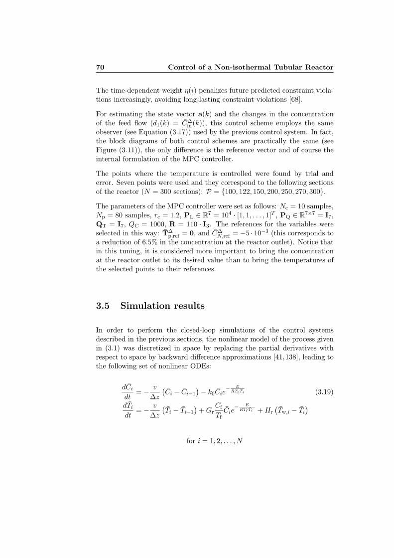
70 Control of a Non-isothermal Tubular Reactor
The time-dependent weight η(i) penalizes future predicted constraint viola-tions increasingly, avoiding long-lasting constraint violations [68].
For estimating the state vector a(k) and the changes in the concentrationof the feed flow (d1(k) = CΔ
in (k)), this control scheme employs the sameobserver (see Equation (3.17)) used by the previous control system. In fact,the block diagrams of both control schemes are practically the same (seeFigure (3.11)), the only difference is the reference vector and of course theinternal formulation of the MPC controller.
The points where the temperature is controlled were found by trial anderror. Seven points were used and they correspond to the following sectionsof the reactor (N = 300 sections): P = {100, 122, 150, 200, 250, 270, 300}.
The parameters of the MPC controller were set as follows: Nc = 10 samples,Np = 80 samples, rc = 1.2, PL ∈ R
7 = 104 · [1, 1, . . . , 1]T , PQ ∈ R7×7 = I7,
QT = I7, QC = 1000, R = 110 · I3. The references for the variables wereselected in this way: TΔ
p,ref = 0, and CΔN,ref = −5 · 10−3 (this corresponds to
a reduction of 6.5% in the concentration at the reactor outlet). Notice thatin this tuning, it is considered more important to bring the concentrationat the reactor outlet to its desired value than to bring the temperatures ofthe selected points to their references.
3.5 Simulation results
In order to perform the closed-loop simulations of the control systemsdescribed in the previous sections, the nonlinear model of the process givenin (3.1) was discretized in space by replacing the partial derivatives withrespect to space by backward difference approximations [41,138], leading tothe following set of nonlinear ODEs:
dCi
dt= − v
Δz
(Ci − Ci−1
)− k0Cie− E
RTf Ti (3.19)
dTi
dt= − v
Δz
(Ti − Ti−1
)+ Gr
Cf
TfCie
− ERTf Ti + Hr
(Tw,i − Ti
)
for i = 1, 2, . . . , N
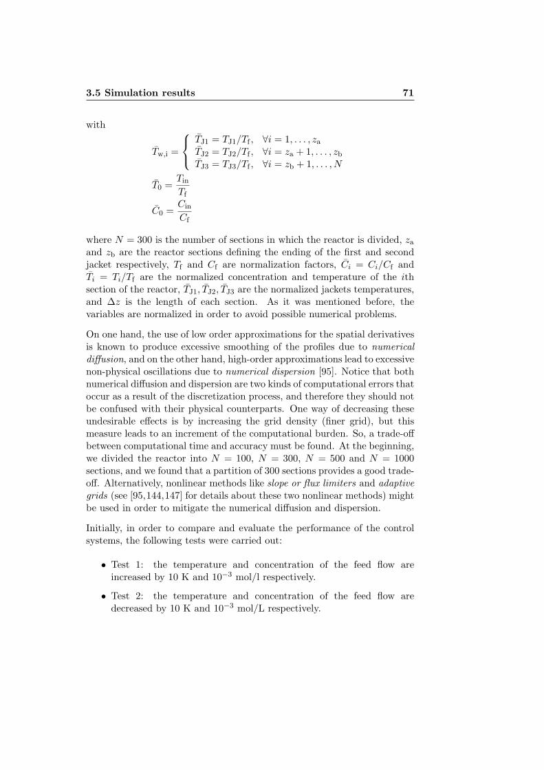
3.5 Simulation results 71
with
Tw,i =
⎧⎨⎩
TJ1 = TJ1/Tf , ∀i = 1, . . . , za
TJ2 = TJ2/Tf , ∀i = za + 1, . . . , zb
TJ3 = TJ3/Tf , ∀i = zb + 1, . . . , N
T0 =Tin
Tf
C0 =Cin
Cf
where N = 300 is the number of sections in which the reactor is divided, za
and zb are the reactor sections defining the ending of the first and secondjacket respectively, Tf and Cf are normalization factors, Ci = Ci/Cf andTi = Ti/Tf are the normalized concentration and temperature of the ithsection of the reactor, TJ1, TJ2, TJ3 are the normalized jackets temperatures,and Δz is the length of each section. As it was mentioned before, thevariables are normalized in order to avoid possible numerical problems.
On one hand, the use of low order approximations for the spatial derivativesis known to produce excessive smoothing of the profiles due to numericaldiffusion, and on the other hand, high-order approximations lead to excessivenon-physical oscillations due to numerical dispersion [95]. Notice that bothnumerical diffusion and dispersion are two kinds of computational errors thatoccur as a result of the discretization process, and therefore they should notbe confused with their physical counterparts. One way of decreasing theseundesirable effects is by increasing the grid density (finer grid), but thismeasure leads to an increment of the computational burden. So, a trade-offbetween computational time and accuracy must be found. At the beginning,we divided the reactor into N = 100, N = 300, N = 500 and N = 1000sections, and we found that a partition of 300 sections provides a good trade-off. Alternatively, nonlinear methods like slope or flux limiters and adaptivegrids (see [95,144,147] for details about these two nonlinear methods) mightbe used in order to mitigate the numerical diffusion and dispersion.
Initially, in order to compare and evaluate the performance of the controlsystems, the following tests were carried out:
• Test 1: the temperature and concentration of the feed flow areincreased by 10 K and 10−3 mol/l respectively.
• Test 2: the temperature and concentration of the feed flow aredecreased by 10 K and 10−3 mol/L respectively.

72 Control of a Non-isothermal Tubular Reactor
0 0.2 0.4 0.6 0.8 1320
340
360
380
400
420
0 0.2 0.4 0.6 0.8 10
0.005
0.01
0.015
0.02
0.025
constraint
Tem
per
atu
re[K
]C
once
ntr
ati
on
[mol/
l]
Length z [m]
Length z [m]
Figure 3.12: Steady-state temperature and concentration profiles of thereactor for Test 1. Dotted line - Nominal profile (reference). Dashed line -MPC-NTC. Solid line - MPC-PV. Dash-dotted line - Open loop response.
0 5 10 15 20 25 30350
352
354
356
358
0 5 10 15 20 25 300
0.5
1
1.5
2x 10
−3
Tem
per
atu
re[K
]C
once
ntr
ati
on
[mol/
l]
t [s]
t [s]
Figure 3.13: Temperature and concentration at the reactor outlet duringTest 1. Dashed line - MPC-NTC. Solid line - MPC-PV. Dash-dotted line -Open loop response.
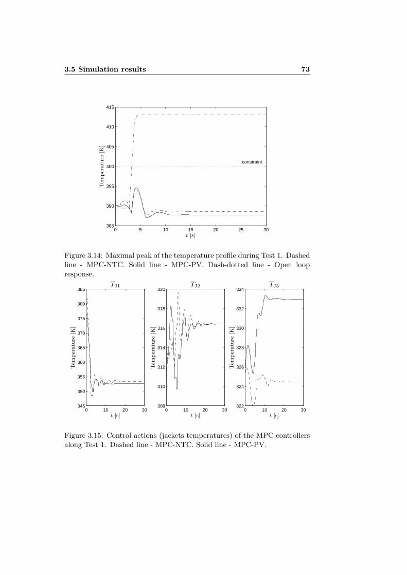
3.5 Simulation results 73
0 5 10 15 20 25 30385
390
395
400
405
410
415
constraint
Tem
per
atu
re[K
]
t [s]
Figure 3.14: Maximal peak of the temperature profile during Test 1. Dashedline - MPC-NTC. Solid line - MPC-PV. Dash-dotted line - Open loopresponse.
0 10 20 30345
350
355
360
365
370
375
380
385
0 10 20 30308
310
312
314
316
318
320
0 10 20 30322
324
326
328
330
332
334
TJ1 TJ2 TJ3
Tem
per
atu
re[K
]
Tem
per
atu
re[K
]
Tem
per
atu
re[K
]
t [s]t [s]t [s]
Figure 3.15: Control actions (jackets temperatures) of the MPC controllersalong Test 1. Dashed line - MPC-NTC. Solid line - MPC-PV.

74 Control of a Non-isothermal Tubular Reactor
0 0.2 0.4 0.6 0.8 10
0.005
0.01
0.015
0.02
0 0.2 0.4 0.6 0.8 1320
340
360
380
400
Tem
per
atu
re[K
]C
once
ntr
ati
on
[mol/
l]
Length z [m]
Length z [m]
Figure 3.16: Steady-state temperature and concentration profiles of thereactor for Test 2. Dotted line - Nominal profile (reference). Dashed line -MPC-NTC. Solid line - MPC-PV. Dash-dotted line - Open loop response.
0 5 10 15 20 25 30348
352
356
360
364
0 5 10 15 20 25 301
2
3
4
5x 10
−3
Tem
per
atu
re[K
]C
once
ntr
ati
on
[mol/
l]
t [s]
t [s]
Figure 3.17: Temperature and concentration at the reactor outlet duringTest 2. Dashed line - MPC-NTC. Solid line - MPC-PV. Dash-dotted line -Open loop response.
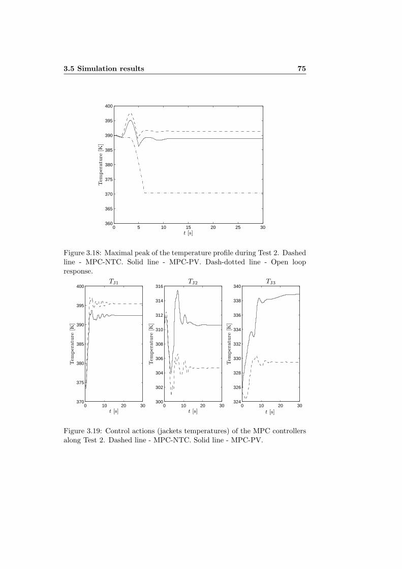
3.5 Simulation results 75
0 5 10 15 20 25 30360
365
370
375
380
385
390
395
400Tem
per
atu
re[K
]
t [s]
Figure 3.18: Maximal peak of the temperature profile during Test 2. Dashedline - MPC-NTC. Solid line - MPC-PV. Dash-dotted line - Open loopresponse.
0 10 20 30370
375
380
385
390
395
400
0 10 20 30300
302
304
306
308
310
312
314
316
0 10 20 30324
326
328
330
332
334
336
338
340TJ1 TJ2 TJ3
Tem
per
atu
re[K
]
Tem
per
atu
re[K
]
Tem
per
atu
re[K
]
t [s]t [s]t [s]
Figure 3.19: Control actions (jackets temperatures) of the MPC controllersalong Test 2. Dashed line - MPC-NTC. Solid line - MPC-PV.

76 Control of a Non-isothermal Tubular Reactor
For carrying out the simulations, we have used as ODE solver the functionODE45 of Matlab. This function is based on an explicit Runge-Kutta (4,5)formula, the Dormand-Prince pair [43]. It is a one step solver that has beenconfigured with a variable integration step and with a relative tolerance of10−5. In order to solve the optimization problem of the MPC controllers,the solver Quadprog has been used. Quadprog is part of the OptimizationToolbox of Matlab [101], and it uses an active set method similar to thatdescribed in [57].
The simulation results of Test 1 are presented in Figures 3.12, 3.13, 3.14and 3.15. Figures 3.16, 3.17, 3.18 and 3.19 show the simulation resultsof Test 2. Furthermore in Table 3.3, some numbers for quantifying theperformance of the control systems are shown. In this table, Tmax is themaximum temperature reached inside the reactor during the test. ΔCout isthe percentage of change of the concentration in steady state at the reactoroutput with respect to its nominal value. That is,
ΔCout(%) =CN − C∗
N
C∗N
× 100 (3.20)
where C∗N is the nominal value (1.5737 · 10−3 mol/l) and CN is the
concentration at the reactor output in steady state after the test.
In Test 1, there is a permanent violation of the temperature constraint (seeFigures 3.12 and 3.14) for the open loop case, which leads to undesirable sidereactions. The maximum temperature value registered is 413.03 K, which isfar from the maximum allowed (400 K). However this temperature incrementin steady state conduces to a reduction of 79.39 % in the concentration at thereactor output. For the case of the MPC control schemes, the temperatureinside the reactor is kept below 400 K, and the concentration at reactoroutlet is reduced a little bit. The control efforts of the MPC controllers canbe observed in Figure 3.15, where it is clear that their control actions areall the time within the boundaries (280 K ≤ TJ1, TJ2, TJ3 ≤ 400 K).
In Test 2, a significant increment of the concentration at the reactor outletis observed when the system is operating in an open loop configuration(see Figures 3.16 and 3.17). We have an increment of 198.25% in steadystate, which means that the performance of the tubular chemical reactor hasbeen reduced dramatically. The MPC controllers overcome this situationby manipulating the temperatures of the jackets in such a way that thetemperature inside the reactor is increased in order to compensate the effectof the input disturbances. We have an increment in the concentration of only

3.5 Simulation results 77
Table 3.3: Performance parameters of the control systems
TestOpen-loop MPC-NTC MPC-PV
ΔCout[%] Tmax[K] ΔCout[%] Tmax[K] ΔCout[%] Tmax[K]1 -79.39 413.03 -0.69 394.09 -0.7 394.592 198.25 390 3.19 397.59 0.63 395.053 -99.46 440.46 52.38 405.08 -6.89 396.624 493.7 390 134 399.67 -54.12 399.34
Tmax [K] = Maximum temperature reached inside the reactor during the test.
ΔCout [%] = Percentage of change of the concentration in steady state at the reactor
output with respect to its nominal value (see Equation (3.20)).
3.19% and 0.63% for the MPC-NTC and MPC-PV controllers respectively.It is clear that the performance of the reactor practically has not beenaffected. Additionally as it is shown in Figure 3.19, the control actionsof both controllers are within the limits.
In general, the control schemes showed a good behavior for rejecting thedisturbances (typical magnitudes: Cin = ±10−3 mol/l and Tin = ±10 K)and both presented a similar performance.
Under the previous tests, the control systems were not operating close to thetemperature constraints, and therefore during the tests, these constraints arenot active in the MPC-PV controller. So, in order to evaluate the abilityof this control scheme of dealing with the temperature constraint along thereactor, the following tests were designed:
• Test 3: the temperature and concentration of the feed flow areincreased by 24 K and 3 · 10−3 mol/l respectively.
• Test 4: the temperature and concentration of the feed flow aredecreased by 30 K and 4 · 10−3 mol/l respectively.
Notice that under these new tests (where the disturbances are too large incomparison with the typical ones) the tubular reactor operates far from theoperating profiles shown in Figure 3.4, and therefore the differences betweenthe nonlinear model of the process and the linear POD model used by thecontrollers are considerable.
The simulation results of Test 3 are given in Figures 3.20, 3.21, 3.22 and

78 Control of a Non-isothermal Tubular Reactor
0 0.2 0.4 0.6 0.8 1320
340
360
380
400
0 0.2 0.4 0.6 0.8 10
0.005
0.01
0.015
0.02
0.025
Tem
per
atu
re[K
]C
once
ntr
ati
on
[mol/
l]
Length z [m]
Length z [m]
Figure 3.20: Steady-state temperature and concentration profiles of thereactor for Test 3. Dotted line - Nominal profile (reference). Dashed line -MPC-NTC. Solid line - MPC-PV.
0 5 10 15 20 25 30 35340
350
360
370
380
390
0 5 10 15 20 25 30 350
1
2
3
4x 10
−3
Tem
per
atu
re[K
]C
once
ntr
ati
on
[mol/
l]
t [s]
t [s]
Figure 3.21: Temperature and concentration at the reactor outlet duringTest 3. Dashed line - MPC-NTC. Solid line - MPC-PV.

3.5 Simulation results 79
0 5 10 15 20 25 30 35375
380
385
390
395
400
405
410
constraint
Tem
per
atu
re[K
]
t [s]
Figure 3.22: Maximal peak of the temperature profile during Test 3. Dashedline - MPC-NTC. Solid line - MPC-PV.
0 7 14 21 28 35260
280
300
320
340
360
380
400
0 7 14 21 28 35260
280
300
320
340
360
380
0 7 14 21 28 35260
280
300
320
340
360
380
400
constraint constraintconstraint
TJ1 TJ2 TJ3
Tem
per
atu
re[K
]
Tem
per
atu
re[K
]
Tem
per
atu
re[K
]
t [s]t [s]t [s]
Figure 3.23: Control actions (jackets temperatures) of the MPC controllersalong Test 3. Dashed line - MPC-NTC. Solid line - MPC-PV.
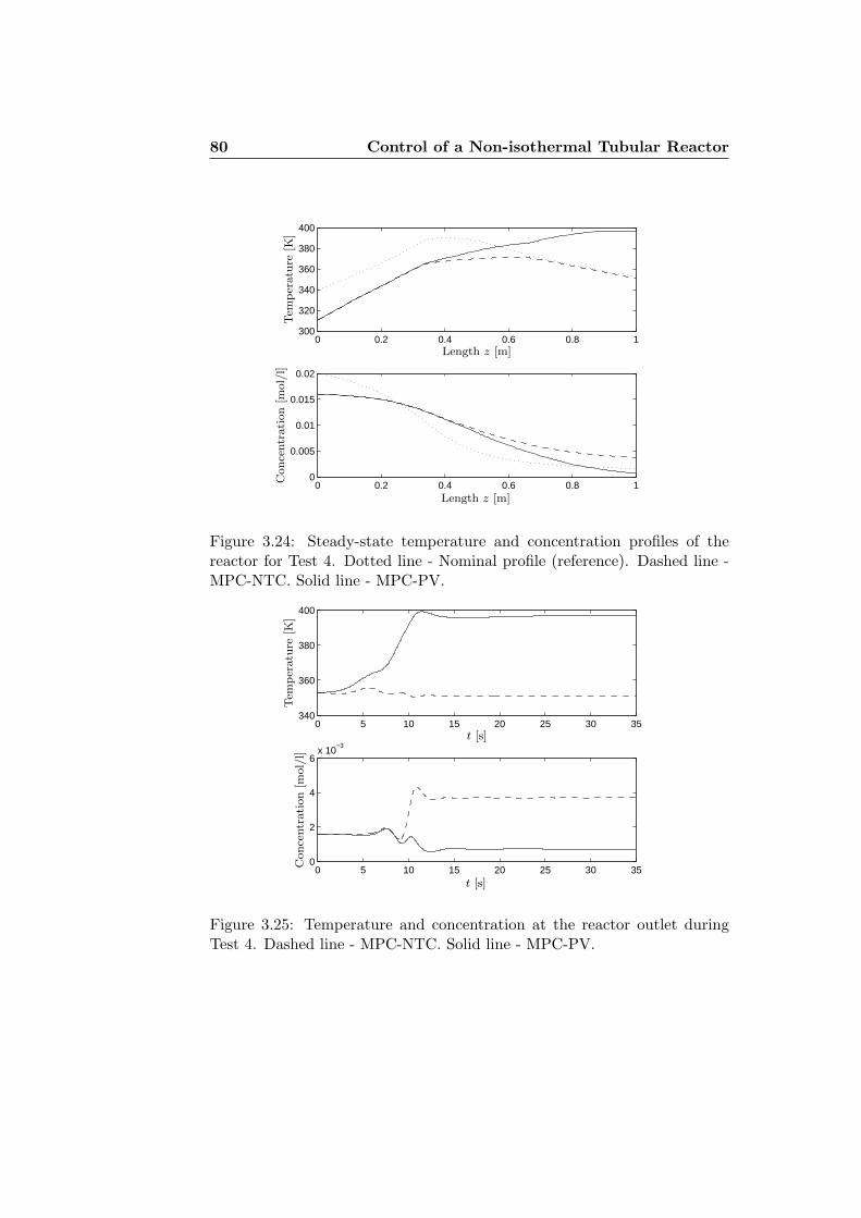
80 Control of a Non-isothermal Tubular Reactor
0 0.2 0.4 0.6 0.8 1300
320
340
360
380
400
0 0.2 0.4 0.6 0.8 10
0.005
0.01
0.015
0.02
Tem
per
atu
re[K
]C
once
ntr
ati
on
[mol/
l]
Length z [m]
Length z [m]
Figure 3.24: Steady-state temperature and concentration profiles of thereactor for Test 4. Dotted line - Nominal profile (reference). Dashed line -MPC-NTC. Solid line - MPC-PV.
0 5 10 15 20 25 30 35340
360
380
400
0 5 10 15 20 25 30 350
2
4
6x 10
−3
Tem
per
atu
re[K
]C
once
ntr
ati
on
[mol/
l]
t [s]
t [s]
Figure 3.25: Temperature and concentration at the reactor outlet duringTest 4. Dashed line - MPC-NTC. Solid line - MPC-PV.

3.5 Simulation results 81
0 5 10 15 20 25 30 35365
370
375
380
385
390
395
400
Tem
per
atu
re[K
]
t [s]
Figure 3.26: Maximal peak of the temperature profile during Test 4. Dashedline - MPC-NTC. Solid line - MPC-PV.
0 7 14 21 28 35360
365
370
375
380
385
390
395
400
405
410
0 7 14 21 28 35260
280
300
320
340
360
380
0 7 14 21 28 35310
320
330
340
350
360
370
380
390
400
constraint
constraint
TJ1 TJ2 TJ3
Tem
per
atu
re[K
]
Tem
per
atu
re[K
]
Tem
per
atu
re[K
]
t [s]t [s]t [s]
Figure 3.27: Control actions (jackets temperatures) of the MPC controllersalong Test 4. Dashed line - MPC-NTC. Solid Line - MPC-PV.

82 Control of a Non-isothermal Tubular Reactor
3.23, and Figures 3.24, 3.25, 3.26 and 3.27 present the simulation resultsof Test 4. In addition, Table 3.3 shows the performance parameters of thecontrol systems.
In Test 3, the MPC-NTC controller violates temporarily the temperatureconstraint as can be observed from Figure 3.22. The constraint is violatedduring 1.46 s and the maximum peak registered is 405.08 K. On the otherhand the MPC-PV controller keeps all the time the temperature profilebelow 400 K. It is important to keep in mind that MPC-NTC does not takeinto account the temperature constraint and the results obtained with it wereexpected. From Table 3.3, it is clear that the performance of the reactoris degraded in a considerable way (the concentration at the reactor outletis increased by 52.38%) for the MPC-NTC case, whereas for the MPC-PVcase the performance of the reactor is increased. Notice in Figure 3.20, howthe last part (particularly when z > 0.667 m) of the temperature profilesis different. The temperature profile of the MPC-PV control scheme isover the profile of the MPC-NTC control system allowing a good reductionof the concentration at the reactor outlet (see also Figure 3.21) for theMPC-PV case. This behavior is the consequence of giving more weightto the concentration (QC = 1000) than to the temperature of the selectedpoints (QT = I7) in the formulation of the MPC-PV controller. The controlactions of both control systems are displayed in Figure 3.23. There aresome temporary saturations of the actuators as a consequence of the largedisturbances, but the control efforts are all the time between 280 K and400 K.
In Test 4, there is no violation of the temperature constraint (see Figure 3.26)when both MPC control systems are used. It is remarkable how MPC-PVreduces the concentration at the reactor outlet by 54.12%. This is not thecase for the MPC-NTC controller where the concentration at the reactoroutput is increased by 134%. In order to compensate the considerabledecrement in the temperature of the feed flow, both controllers try toincrease the temperature of the first jacket as much as possible, in this caseuntil 400 K (actuator upper limit). This can be observed in Figure 3.27.
From the previous two tests, it is evident that MPC-PV notably outperformsMPC-NTC when large disturbances are applied to the reactor. At this pointit is important to remark that the MPC-PV controller was somehow favoredby the differences between the nonlinear model of the process and the linearPOD model on which it is based. This observation can be corroborated bythe fact that the controller was set to reduce the concentration at the reactor

3.5 Simulation results 83
outlet by 6.5% and not by 54.12% as happened in Test 4 for instance. Itis remarkable how the MPC-PV controller can deal with the temperatureconstraint of the system in spite of using a linear POD model of the tubularreactor.
3.5.1 Tests on a reactor with axial dispersion
In order to include the axial dispersion phenomena in the plug flow reactormodel (3.1), second-order dispersion terms have to be added as follows:
∂C
∂t= DC
∂2C
∂z2− v
∂C
∂z− k0Ce−
ERT (3.21a)
∂T
∂t= DT
∂2C
∂z2− v
∂T
∂z+ GrCe−
ERT + Hr(Tw − T ) (3.21b)
where DC and DT are the mass and energy dispersion coefficients in [m2/s].Note, however, that in practice the dimensionless mass and energy Pecletnumbers, i.e., PeC = vL/DC, and PeT = vL/DT, are mostly used forindicating the level of dispersion. The boundary conditions of the previousPDEs are the classical Danckwerts boundary conditions [39] given by
DC∂C
∂z= v (C − Cin) at z = 0 (3.22a)
DT∂T
∂z= v (T − Tin) at z = 0 (3.22b)
∂C
∂z= 0 at z = L (3.22c)
∂T
∂z= 0 at z = L. (3.22d)
For carrying out the closed-loop simulations of the MPC-NTC and MPC-PV controllers with the dispersive plug flow reactor model, the nonlinearmodel (3.21) was discretized in space by using a finite difference method.So, the second and first partial derivatives with respect to z were replaced bycentral difference approximations and backward difference approximationsrespectively, leading to the following set of nonlinear ODEs:
dCi
dt=
DC
Δz2
(Ci+1 + Ci−1 − 2Ci
)− v
Δz
(Ci − Ci−1
)− k0Cie− E
RTf Ti (3.23)
dTi
dt=
DT
Δz2
(Ti+1 + Ti−1 − 2Ti
)− v
Δz
(Ti − Ti−1
)+
+ GrCf
TfCie
− ERTf Ti + Hr
(Tw,i − Ti
)

84 Control of a Non-isothermal Tubular Reactor
for i = 1, 2, . . . , N
with
Tw,i =
⎧⎨⎩
TJ1 = TJ1/Tf , ∀i = 1, . . . , za
TJ2 = TJ2/Tf , ∀i = za + 1, . . . , zb
TJ3 = TJ3/Tf , ∀i = zb + 1, . . . , N
T0 =1
DT + vΔz
(vΔz
Tin
Tf+ DTT1
)
C0 =1
DC + vΔz
(vΔz
Cin
Cf+ DCC1
)TN+1 = TN
CN+1 = CN
where N = 300 is the number of sections in which the reactor is divided, za
and zb are the reactor sections defining the ending of the first and secondjacket respectively, Tf and Cf are normalization factors, Ci = Ci/Cf andTi = Ti/Tf are the normalized concentration and temperature of the ithsection of the reactor, TJ1, TJ2, TJ3 are the normalized jackets temperatures,and Δz is the length of each section.
For the sake of simplicity, in this study it is assumed that the mass andenergy dispersion coefficients are equal, that is, DC = DT = D (PeC = PeT =Pe). In Figure 3.28 we can observe the effect of increasing the dispersioncoefficient D on the steady-state profiles of the reactor derived by means ofthe optimization algorithm presented in Section 3.2.2 (in Figure 3.28, casewhen D = 0 or equivalently Pe = ∞). It is clear that as the dispersioncoefficient increases, the dispersion induces lower temperatures inside thereactor, which decreases the magnitude of the hot spot but inevitablydegrades the reactor performance. For D = 0.001 m2/s (Pe = 100) andD = 0.005 m2/s (Pe = 20), the concentration at the reactor outlet isincreased by 22.48% and 79.8% respectively (these increments are measuredwith respect to the concentration at the reactor outlet when D = 0). Noticealso, that as the dispersion coefficient D grows, the difference betweenthe feed values (Cin = 0.02 mol/l and Tin = 340 K) and the inlet values(C(z = 0) and T (z = 0)) increases according to the Danckwerts boundaryconditions.
Tests 1 and 2 were carried out again, but this time the predictive controllerswere attached to the dispersive plug flow reactor model (3.21). The factof using a dispersive tubular reactor constitutes a way of evaluating the
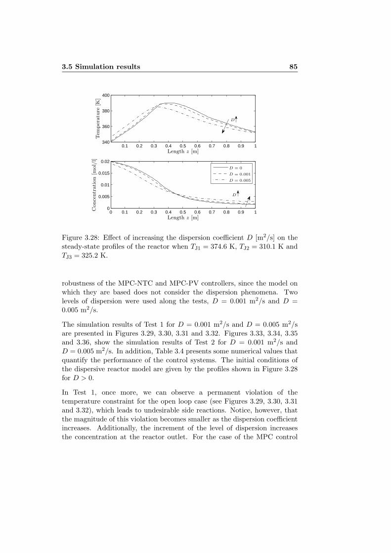
3.5 Simulation results 85
0.1 0.2 0.3 0.4 0.5 0.6 0.7 0.8 0.9 1340
360
380
400
0 0.1 0.2 0.3 0.4 0.5 0.6 0.7 0.8 0.9 10
0.005
0.01
0.015
0.02
Tem
per
atu
re[K
]C
once
ntr
ati
on
[mol/
l]
Length z [m]
Length z [m]
D
D
D = 0
D = 0.001
D = 0.005
Figure 3.28: Effect of increasing the dispersion coefficient D [m2/s] on thesteady-state profiles of the reactor when TJ1 = 374.6 K, TJ2 = 310.1 K andTJ3 = 325.2 K.
robustness of the MPC-NTC and MPC-PV controllers, since the model onwhich they are based does not consider the dispersion phenomena. Twolevels of dispersion were used along the tests, D = 0.001 m2/s and D =0.005 m2/s.
The simulation results of Test 1 for D = 0.001 m2/s and D = 0.005 m2/sare presented in Figures 3.29, 3.30, 3.31 and 3.32. Figures 3.33, 3.34, 3.35and 3.36, show the simulation results of Test 2 for D = 0.001 m2/s andD = 0.005 m2/s. In addition, Table 3.4 presents some numerical values thatquantify the performance of the control systems. The initial conditions ofthe dispersive reactor model are given by the profiles shown in Figure 3.28for D > 0.
In Test 1, once more, we can observe a permanent violation of thetemperature constraint for the open loop case (see Figures 3.29, 3.30, 3.31and 3.32), which leads to undesirable side reactions. Notice, however, thatthe magnitude of this violation becomes smaller as the dispersion coefficientincreases. Additionally, the increment of the level of dispersion increasesthe concentration at the reactor outlet. For the case of the MPC control

86 Control of a Non-isothermal Tubular Reactor
Table 3.4: Performance parameters of the control systems
TestD Open-loop MPC-NTC MPC-PV
[m2/s] ΔCout Tmax ΔCout Tmax ΔCout Tmax
10 -79.39 413.03 -0.69 394.09 -0.7 394.59
0.001 -71.35 411.6 24.21 390.3 10.04 389.50.005 -35.18 404.3 97.82 385.6 11.41 390.44
20 198.25 390 3.19 397.59 0.63 395.05
0.001 211.4 388.6 38.5 390.48 8.43 389.130.005 261.7 384.98 153.1 384.99 1.87 399.42
Tmax [K] = Maximum temperature reached inside the reactor during the test.
ΔCout [%] = Percentage of change of the concentration in steady state at the reactor
outlet with respect to 1.5737 · 10−3 mol/l (see Equation (3.20)).
schemes, the temperature inside the reactor is kept below 400 K. From Table3.4, it is clear that the MPC-NTC controller is not as good as the MPC-PVcontroller for keeping the concentration at the reactor outlet close to itsnominal value.
In Test 2, the reactor conversion is notably reduced when the system isoperating in an open-loop configuration. This situation becomes more andmore critical as the level of dispersion increases (see Figures 3.33 and 3.34and Table 3.4). In order to counteract the effect of the input disturbances,the predictive controllers manipulate the jackets temperatures in such away that the temperature inside the reactor is increased. From the resultsobtained, it is clear that the MPC-PV controller does a much better job thanthe MPC-NTC controller, which loses performance when the dispersion inthe reactor is increased.
In general, the presence of dispersion in the reactor has had a muchbigger impact on the performance of the MPC-NTC controller than onthe performance of the MPC-PV controller. As the dispersion increases,the MPC-NTC controller loses its ability of keeping the concentration atthe reactor outlet close to its nominal value. So, it is clear that forimproving the behavior of this controller, it would be necessary to includethe dispersion phenomena in the POD model on which this controller isbased. Furthermore, the nonlinearities of the reactor contribute to the poorperformance exhibited by the MPC-NTC controller, since under dispersiveconditions the reactor can operate far away from the nominal operating

3.5 Simulation results 87
0 0.2 0.4 0.6 0.8 1340
360
380
400
420
0 0.2 0.4 0.6 0.8 10
0.005
0.01
0.015
0.02
0.025
constraint
Tem
per
atu
re[K
]C
once
ntr
ati
on
[mol/
l]
Length z [m]
Length z [m]
Figure 3.29: Steady-state profiles of the reactor with D = 0.001 m2/s forTest 1. Dotted line - Nominal profile (reference). Dashed line - MPC-NTC.Solid line - MPC-PV. Dash-dotted line - Open loop response.
0 0.2 0.4 0.6 0.8 1340
360
380
400
420
0 0.2 0.4 0.6 0.8 10
0.005
0.01
0.015
0.02
0.025
constraint
Tem
per
atu
re[K
]C
once
ntr
ati
on
[mol/
l]
Length z [m]
Length z [m]
Figure 3.30: Steady-state profiles of the reactor with D = 0.005 m2/s forTest 1. Dotted line - Nominal profile (reference). Dashed line - MPC-NTC.Solid line - MPC-PV. Dash-dotted line - Open loop response.

88 Control of a Non-isothermal Tubular Reactor
0 5 10 15 20 25 30 35380
385
390
395
400
405
410
415
constraint
Tem
per
atu
re[K
]
t [s]
Figure 3.31: Maximal peak of the temperature profile during Test 1 whenD = 0.001 m2/s. Dashed line - MPC-NTC. Solid line - MPC-PV. Dash-dotted line - Open loop response.
0 10 20 30 40 50 60 70370
375
380
385
390
395
400
405
constraint
Tem
per
atu
re[K
]
t [s]
Figure 3.32: Maximal peak of the temperature profile during Test 1 whenD = 0.005 m2/s. Dashed line - MPC-NTC. Solid line - MPC-PV. Dash-dotted line - Open loop response.

3.5 Simulation results 89
0 0.2 0.4 0.6 0.8 1320
340
360
380
400
0 0.2 0.4 0.6 0.8 10
0.005
0.01
0.015
0.02
Tem
per
atu
re[K
]C
once
ntr
ati
on
[mol/
l]
Length z [m]
Length z [m]
Figure 3.33: Steady-state profiles of the reactor with D = 0.001 m2/s forTest 2. Dotted line - Nominal profile (reference). Dashed line - MPC-NTC.Solid line - MPC-PV. Dash-dotted line - Open loop response.
0 0.2 0.4 0.6 0.8 1320
340
360
380
400
0 0.2 0.4 0.6 0.8 10
0.005
0.01
0.015
0.02
Tem
per
atu
re[K
]C
once
ntr
ati
on
[mol/
l]
Length z [m]
Length z [m]
Figure 3.34: Steady-state profiles of the reactor with D = 0.005 m2/s forTest 2. Dotted line - Nominal profile (reference). Dashed line - MPC-NTC.Solid line - MPC-PV. Dash-dotted line - Open loop response.

90 Control of a Non-isothermal Tubular Reactor
0 5 10 15 20 25 30 35365
370
375
380
385
390
395
Tem
per
atu
re[K
]
t [s]
Figure 3.35: Maximal peak of the temperature profile during Test 2 whenD = 0.001 m2/s. Dashed line - MPC-NTC. Solid line - MPC-PV. Dash-dotted line - Open loop response.
0 10 20 30 40 50365
370
375
380
385
390
395
400
Tem
per
atu
re[K
]
t [s]
Figure 3.36: Maximal peak of the temperature profile during Test 2 whenD = 0.005 m2/s. Dashed line - MPC-NTC. Solid line - MPC-PV. Dash-dotted line - Open loop response.

3.6 Conclusions 91
profiles (see Figure 3.28, case when D = 0 m2/s) where the linear PODmodel provides a suitable approximation of the nonlinear model of thesystem.
Observe in Figures 3.29, 3.30, 3.33 and 3.34, how the MPC-PV controllerincreases the temperature of the last sections of the reactor in order toguarantee a good performance of the system. As it was explained before,this behavior is the consequence of giving more importance to the reductionof the concentration at the rector outlet than to the reduction of thetemperature deviations in the formulation of the predictive controller.It is remarkable how the MPC-PV controller is able to maintain theconcentration at the reactor outlet close to its nominal value, in spite ofusing a POD model that does not incorporate both the dispersion effectsand the nonlinearities of the system.
Although it is not shown in this section, the control efforts of the predictivecontrollers were all the time within the boundaries (280 K ≤ TJ1, TJ2, TJ3 ≤400 K).
3.6 Conclusions
In this chapter we have presented the results of applying POD and predictivecontrol techniques to the control of the temperature and concentrationprofiles of a non-isothermal tubular reactor. In addition, we have in-troduced an optimization algorithm for deriving the operating profiles ofthe process. Thanks to the POD and Galerkin projection techniques,the high-dimensionality of the linearized model of the reactor has beensignificantly reduced making possible the control design. Two POD-basedMPC control schemes have been proposed: a scheme where the formulationof the predictive controller is in terms of the POD coefficients (MPC-NTC) and a scheme where the MPC is formulated in terms of physicalvariables (MPC-PV). In the first case, the control of the reactor profilesis achieved indirectly by controlling the POD coefficients which have nophysical meaning. This makes the tuning of the controller little intuitiveand the definition of the control goals little flexible. This is not the casefor the second MPC controller where its formulation is in terms of thetemperature of some selected points along the reactor and the concentrationat the reactor output. Taking advantage of the flexibility that this schemeprovides, we gave more importance to the reduction of the concentration at

92 Control of a Non-isothermal Tubular Reactor
the reactor outlet than to the reduction of the temperature deviations. Asa consequence of this setting, we observed in the simulation results how thiscontrol system outperforms the first one when large disturbances are appliedto the plant. Notice however that under typical disturbances (Test 1 and2), both control systems practically exhibit a similar performance. In testswith a dispersive tubular reactor, the second control scheme outperformedonce more the MPC formulated in terms of the POD coefficients.
Unlike the first control scheme, the MPC formulated in terms of physicalvariables imposes the temperature constraint of the reactor (T (z, t) ≤400 K) in some selected points of the spatial domain. It was argued thatimposing the temperature constraint in some specific points might indirectlyenforce this constraint in the remaining points given the smoothness of thetemperature profile and the limited number of jackets. The simulationresults showed that the controller was able to reject large disturbanceswithout letting this constraint be violated. Nevertheless, the most difficultpart in the tuning of this controller is the selection of the points where thetemperature constraint is imposed. In this study, such selection was done bytrial and error and therefore we had to carry out a lot of simulations in orderto find a suitable set of points. This is of course not practical since a lotof time and computational resources are needed. In Section 4.4 of the nextchapter, we present a way of finding a suitable set of points by means of agreedy selection algorithm. The reader is referred to the end of this sectionwhere we also discuss an improved formulation of the MPC-PV controller.
Given that the MPC-NTC controller does not take into account thetemperature constraint of the reactor, a temporary violation of thisconstraint was observed during Test 3. In the next chapter, we propose anextension of this controller which incorporates the temperature constraintin its formulation. We will see that this new MPC will have to deal witha very large number of linear inequality constraints (24 000). Since sucha large number of constraints demands a considerable amount of memoryand computational time for solving the optimization problem of the MPCcontroller, in the next chapter we propose two approaches for reducing orapproximating this large number of inequality constraints.
Finally, it is important to remark that the tuning of the controllers havebeen done in a conservative way in order to let them deal with large inputdisturbances. We have to keep in mind that under large disturbances in thefeed flow (Tests 3 and 4), the reactor operates far from its nominal operatingprofiles and therefore the differences between the linear POD model used by

3.6 Conclusions 93
the controllers and the nonlinear model of the reactor are considerable. Itshould be clear that if a tight tuning is required, it would be necessary toincorporate the nonlinear characteristics of the reactor into the POD model.

94 Control of a Non-isothermal Tubular Reactor

Chapter 4
Constraint Handling
4.1 Introduction
In the previous chapter, two POD-based predictive controllers were pro-posed for controlling the temperature and concentration profiles of a non-isothermal tubular chemical reactor. The control goal was to reject thedisturbances that affect the process, that is, the changes in the temperatureand concentration of the feed flow. One important constraint of the systemis that the temperature inside the reactor must be below a given value inorder to prevent undesirable side reactions. Under typical disturbances, thecontroller formulated in terms of the POD coefficients, which is referred to asMPC-NTC (described by (3.16)), performs very well, and the temperatureconstraint is not violated despite the fact that the predictive controllerdoes not incorporate this constraint in its formulation. However, iflarger disturbances are applied, temporary violations of this constraint areobserved.
In this chapter we start by presenting an extension of the MPC-NTCcontroller proposed in Section 3.4.1. This new POD-based controller takesinto account the temperature constraint of the reactor and uses a slackvariable approach with �∞-norm and time-dependent weights for handlingthe infeasibilities that can arise [68]. Given that POD only reduces thenumber of states and not the number of temperature constraints whichusually is very large, the optimization problem posed by this MPC, demandsa considerable amount of memory and requires more computational time.
95

96 Constraint Handling
In this chapter we present two techniques for reducing the number oftemperature constraints. In the first technique, we approximate thefeasible region delimited by the large set of temperature constraints (linearinequalities) by means of the theory of positive polynomials [1]. Thisapproximation leads to a reduction in the number of constraints by replacingmany linear inequalities by a few Linear Matrix Inequalities (LMIs) and asmall number of linear equalities. In this method the MPC optimizationproblem is written as a Semidefinite Program (SDP). In the secondapproach, we propose a greedy algorithm that exploits the similaritiesbetween the coefficients of consecutive constraints for selecting a reduced setof them [5], and unlike the first approach the MPC optimization problemis written as a Quadratic Program (QP). These approaches are some of themain contributions of this dissertation.
Based on the polynomial approximation of the temperature constraints, andbased on the reduced set of constraints found by the greedy algorithm, twonew predictive controllers are devised. These controllers also incorporatethe mechanism for handling infeasibilities mentioned before.
This chapter is structured as follows. Section 4.2 presents the extensionof the MPC-NTC controller, that is, a POD-based MPC controller thatdeals with a very large number of temperature constraints. In Section 4.3,our method for approximating the temperature constraints by using thetheory of positive polynomials is described, and a new MPC is presented.Furthermore, the basics of this theory are discussed and some simulationresults are shown. Section 4.4 presents our greedy selection algorithm forreducing the number of temperature constraints. Additionally, we showsome simulation results. Finally in Section 4.5, we summarize and concludethis chapter.
4.2 POD-based MPC controller with temperatureconstraints
In this section we present an extension of the control scheme describedin Section 3.4.1, which takes into account the temperature constraint ofthe reactor and incorporates a mechanism for dealing with infeasibilities.As it was explained in Section 3.4.1, the control of the temperatureand concentration profiles is achieved indirectly by controlling the POD

4.2 POD-based MPC controller with temperature constraints 97
coefficients, whose references aref are given by
aref = ΦTnxref
where xref is the reference of the state vector x(t) and is equal to 0 since thecontrol system has to keep the reactor operating around the profiles shownin Figure 3.4.
As it was stated in Section 3.4.2, the fact of taking into account thetemperature constraint of the reactor, creates the necessity of establishing amechanism for handling the infeasibilities that can come out due to thedifferences between the process and the model used by the MPC, themagnitude of the disturbances, the saturation of the actuators, and soon. In this MPC formulation, we treat the temperature constraint as asoft constraint by using a slack variable approach with �∞-norm and time-dependent weights [68,69]. This MPC, which will be referred to as MPC-QP,is formulated as follows:
minaNp ,ΔuNc ,dNp ,ξ
Np∑i=1
‖aref(k + i) − a(k + i)‖2Q +
Nc−1∑i=0
‖Δu(k + i)‖2R+ (4.1a)
+PQξ2 + PLξ
subject to
a(k + i + 1) = Aa(k + i) + Bu(k + i) + Fd(k + i), i = 0, . . . , Np − 1,
d(k + i + 1) = d(k + i), i = 0, . . . , Np − 1,
u(k + i) = u(k + i − 1) + Δu(k + i), i = 0, . . . , Nc − 1,
u(k + i) = u(k + i − 1), i = Nc, . . . , Np − 1,
umin ≤ u(k + i) ≤ umax, i = 0, . . . , Nc − 1,
TΔ(k + i) = ΦTa(k + i) ≤ TΔmax + 1 · η(i)ξ, i = 1, . . . , Np, (4.1b)ξ ≥ 0, (4.1c)
with
aNp = [a(k + 1); a(k + 2); . . . ; a(k + Np)]dNp = [d(k + 1); d(k + 2); . . . ; d(k + Np)]
ΔuNc = [Δu(k); Δu(k + 1); . . . ; Δu(k + Nc − 1)]

98 Constraint Handling
where Q and R are weighting matrices (Q � 0,R 0), ‖v‖2Q denotes vTQv,
Np is the prediction horizon, Nc is the control horizon, umin and umax are thelower and upper bounds (these hard constraints are necessary due to physicallimitations of the actuators) of u(k), ΦT is the lower part (the last N = 300rows) of the matrix Φn =
[ΦT
C,ΦTT
]T that is associated to the temperatureprofile, TΔ(k) = ΦTa(k) is a vector which contains the normalizeddeviations of the temperature profile, TΔmax = (400 K · 1 − T∗) /Tf is avector that contains the maximal allowed temperature for each point of thereactor, ξ is the slack variable (a scalar quantity), PQ and PL are weightingfactors (PQ > 0, PL > 0), 1 ∈ R
300 is a vector of 1’s and η(i) = 1/ri−1c , is a
time-dependent weight (rc > 1).
In this formulation the maximum violation of the temperature constraintalong the reactor and the prediction horizon is penalized by means of theterm PQξ2 +PLξ. A sufficiently large PL will ensure that the constraints areenforced as exact soft constraints, that is, that constraint violations will onlyoccur when there is no feasible solution of the original problem [68]. Thequadratic term PQξ2 is used as an additional tuning parameter and it alsoleads to a well-posed quadratic program (positive definite Hessian) [131].
The time-dependent weight η(i) is used for penalizing future predictedconstraint violations increasingly, avoiding long-lasting constraint violations[68].
Similarly to the MPC controllers presented in the previous chapter, thiscontroller is embedded in the same block diagram depicted in Figure 3.11(case MPC-NTC), and it uses the Kalman filter described by (3.17) forestimating the state vector a(k) of the POD model (3.14) and the changesin the concentration of the feed flow (d1(k) = CΔ
in (k)).
The control horizon Nc was set to 10 samples and the prediction horizonNp was selected according to the following criterion: “Prediction Horizon= Control Horizon + Largest Settling Time = 80 samples”. umin and umax
were selected according to the input constraints of the process and theoperating temperatures of the jackets. The other parameters were selectedas follows: rc = 1.2, PL = 104, PQ = 104, Q = I20 and R = 110 · I3.
The optimization problem (4.1) that is solved by the MPC controller is aquadratic programming (QP) problem which has N × Np = 300 × 80 =24 000 temperature constraints. This amount of constraints demands aconsiderable amount of memory and computing power. Although the POD

4.3 Positive polynomial approach 99
technique has reduced the number of state variables of the high-dimensionalmodel (3.8), the number of temperature constraints is still very large.
In the next sections, we present two approaches for tackling this problem.Initially, we introduce an interesting approach which uses the positivepolynomials theory for replacing the large number of inequalities by a fewlinear matrix inequalities while maintaining a control of the temperatureat every point at the reactor (infinity number of points). Afterwards, wepresent a greedy selection algorithm which reduces the number of constraintsby choosing properly only some of them. Note however that unlike thepositive polynomial approach, in this method we do not have any commandon the temperature between the discretization points.
4.3 Positive polynomial approach
4.3.1 Fundamentals
Many specific problems, particularly in systems and control, can be reducedto the verification of the global nonnegativity of a polynomial function [28].In [117] some examples are provided, namely, Lyapunov function computa-tion, output feedback stabilization, multidimensional system stability, etc.
The Tarski-Seidenberg decision procedure described in [27,28,106], providesan explicit algorithm for deciding if a polynomial is nonnegative, so it isclear that this problem is decidable. In addition, there are some alternativeapproaches based on decision algebra like the ones discussed in [18,28].
In general, the problem of testing the global nonnegativity of a multivariatepolynomial function is in fact Nondeterministic Polynomial-time hard (NP-hard), when its degree is larger or equal than four [117]. So, in order toavoid the complexity problems of the previous methods which provide anexact solution to this problem, we have to look for relaxed conditions thatcan be efficiently tested while guaranteeing the global nonnegativity of thepolynomial.
An obvious necessary condition for the nonnegativity of a polynomial is thatits degree has to be even. Now, a simple sufficient condition for a real-valuedpolynomial G(x1, . . . , xl) = G(x) : R
l → R to be nonnegative everywhere isgiven by the existence of its Sum Of Squares (SOS) decomposition defined

100 Constraint Handling
as follows,
G(x) =m∑
j=1
g2j (x) (4.2)
where gj(x) = gj(x1, . . . , xl) ∀j = 1, . . . , m are real-valued polynomials inx1, . . . , xl. Notice however that in general, SOS is not equivalent to thenonnegativity of a polynomial. Only in the following special cases theyare equivalent: quadratic polynomials, univariate polynomials and quarticpolynomials in two variables.
Further, the SOS representability of a polynomial can be expressed as asemidefinite feasibility problem [111,117], as the following proposition states.
Proposition 4.1. A multivariate polynomial G(x) of degree 2d is SOS ifand only if there exists a positive semidefinite matrix W and a vector ofmonomials h(x) containing monomials in x1, . . . , xl of degree ≤ d such that
G(x) = h(x)TW h(x). (4.3)
The number of components of h(x) is given by„
d + ld
«and the number of
squares m in (4.2) is equal to the rank of W, which in general is not unique.
Example 4.1 ( [115,117]). In this example, we are interested in finding outwhether or not the quartic (2d = 4) polynomial in two variables G(x1, x2) =2x4
1 + 2x31x2 − x2
1x22 + 5x4
2 is SOS.
First of all, let us define h(x1, x2) as follows: h(x1, x2) =[x2
1, x22, x1x2
]T .We can write G(x1, x2) in the following quadratic form:
G(x1, x2) = 2x41 + 2x3
1x2 − x21x
22 + 5x4
2
=
⎡⎣ x2
1
x22
x1x2
⎤⎦T ⎡⎣ w11 w12 w13
w12 w22 w23
w13 w23 w33
⎤⎦⎡⎣ x2
1
x22
x1x2
⎤⎦
= w11x41 + w22x
42 + (2w12 + w33)x2
1x22 + 2w13x
31x2 + 2w23x1x
32.
By equating the coefficients of G(x1, x2) to the coefficients of the monomialsobtained from expanding h(x1, x2)TW h(x1, x2), we obtain the followingset of affine relations:
w11 = 2,
4.3 Positive polynomial approach 101
w22 = 5,
w13 = 1,
w23 = 0,
2w12 + w33 = −1.
A positive semidefinite matrix W � 0 that satisfies the previous linearequalities can then be found by using semidefinite programming. Aftersolving numerically, we obtained the following particular solution:
w12 = −3,
w33 = 5,
W =
⎡⎣ 2 −3 1
−3 5 01 0 5
⎤⎦ � 0.
This is a certificate that G(x1, x2) is nonnegative everywhere since G(x1, x2)is SOS. Given that the rank of W is 2, we have only 2 squares in the SOSdecomposition. If we want to compute the SOS decomposition of G(x1, x2)we proceed as follows. First we calculate the Cholesky factorization of W,
W = UTc Uc, where Uc =
1√2
[2 −3 10 1 3
],
and finally, we substitute the previous factorization into the quadratic formof G(x1, x2),
G(x1, x2) = h(x1, x2)TUTc Uc h(x1, x2)
= ‖Uc h(x1, x2)‖22
=∥∥∥∥ 1√
2
[2x2
1 − 3x22 + x1x2
x22 + 3x1x2
]∥∥∥∥2
2
=12(2x2
1 − 3x22 + x1x2
)2 +12(x2
2 + 3x1x2
)2.
As it was mentioned at the beginning of this section, checking thenonnegativity of a polynomial G(x) is an NP-hard problem when the degreeof G(x) is at least 4 [108], whereas checking whether G(x) can be written asan SOS is computationally tractable, since it can be formulated as an SDPproblem which in the worst case has a polynomial time complexity. Althoughwe are not going into details, there are several results that suggest that this

102 Constraint Handling
relaxation is not too conservative [124]. Observe that when we increase thenumber of variables or the degree of G(x), the computational complexity fortesting whether or not G(x) is SOS also increases. Even so, the complexityoverload is still a polynomial function of these parameters [115].
4.3.2 Approximation of the temperature constraints by meansof positive polynomials
In spite of the fact that the POD model of the reactor has 20 states, in thischapter a 2nd order POD model is used for visualizing the feasible regionsdelimited by the temperature constraints and explain the main ideas of boththis positive polynomial approach and the technique based on the greedyselection algorithm.
Figure 4.1 shows in dashed line the feasible region delimited by thetemperature constraints
ΦTa(k) ≤ TΔmax (4.4)
of a 2nd order POD model.
As it was mentioned before, ΦT ∈ R300×20 is the lower part of the matrix
Φn =[ΦT
C,ΦTT
]T , therefore each column of ΦT corresponds to the part of thebasis vectors ϕj ∀j = 1, 2, . . . , n = 20 that is associated to the temperatureprofile. That is,
ΦT =[ϕ1, ϕ2, . . . , ϕj , . . . , ϕ20
],
where ϕj ∈ R300 for j = 1, 2, . . . , n = 20.
In this thesis we use the term “smoothness” to indicate that a functiondoes not change abruptly and/or that it does not oscillate too much (lowfrequency content). By taking advantage of the smoothness of the mostrelevant columns of ΦT, we can find polynomial approximations Pj(z) ofthe vectors ϕj ∀j = 1, 2, . . . , 20 by means of a least squares regression.These approximations would satisfy:
Pj(zi) ≈ ϕij ∀j = 1, 2, . . . , n = 20, (4.5a)
Pmax(zi) ≈ TΔmaxi (4.5b)
for i = 1, 2, . . . , N = 300,
where ϕij is the ith element of ϕj associated to the ith grid point, TΔmaxi is
the ith element of TΔmax associated to the ith grid point, Pj(z) and Pmax(z)

4.3 Positive polynomial approach 103
0 50 100−40
−20
0
20
40
60
80degree 2
0 50 100−40
−20
0
20
40
60
80degree 4
0 50 100−40
−20
0
20
40
60
80degree 8
0 50 100−40
−20
0
20
40
60
80degree 10
feasible region
a1(k)a1(k)
a1(k)a1(k)
a2(k
)
a2(k
)
a2(k
)
a2(k
)
Figure 4.1: Feasible regions delimited by the temperature constraints ofa 2nd order POD model. Dashed line - Original temperature constraints.Solid line - Polynomial approximations of different degree given by (4.6).Solid line with dots - Polynomial approximations of different degree givenby (4.9).
are univariate real polynomials of degree d that approximate the vectors ϕj
and TΔmax respectively, z is the spatial coordinate and zi = iΔz is the valueof the spatial coordinate at the ith grid point.
By using Equations (4.5a) and (4.5b) we can approximate Equation (4.4)by
ΦTa(k) ≤ TΔmax (4.6)
with
ΦT =
⎡⎢⎢⎢⎣
P1(z1) P2(z1) · · · Pn(z1)P1(z2) P2(z2) · · · Pn(z2)
......
. . ....
P1(zN ) P2(zN ) · · · Pn(zN )
⎤⎥⎥⎥⎦

104 Constraint Handling
TΔmax =
⎡⎢⎢⎢⎣
Pmax(z1)Pmax(z2)
...Pmax(zN )
⎤⎥⎥⎥⎦
where ΦT and TΔmax are the approximations of ΦT and TΔmax respectively,N = 300 is the number of sections into which the reactor is divided (numberof grid points) and n = 20 is the number of the selected POD basis vectors.
Figure 4.1 shows the feasible regions (in solid line) delimited by Equation(4.6) for a 2nd order POD model when polynomials of different degree areused. From this Figure, it is clear that polynomials of degree 10 are accurateenough for approximating ϕj ∀j = 1, 2 and TΔmax .
Equation (4.6) imposes the temperature constraint only on the grid pointsof the interval [0, 1]. However, we can impose the condition (4.6) on everypoint of the interval [0, 1], giving
n∑j=1
aj(k)Pj(z) ≤ Pmax(z), ∀z ∈ [0, 1]
which can be rewritten by defining
P (k)(z) = Pmax(z) −n∑
j=1
aj(k)Pj(z)
as follows:P (k)(z) ≥ 0, ∀z ∈ [0, 1]. (4.7)
The resulting polynomial P (k)(z) of degree d has to be nonnegative, at leastin the interval z ∈ [0, 1].
Even though we have now seemingly complicated the problem by replacingmany by infinitely many inequalities, this new formulation can efficiently behandled by positive polynomials techniques.
4.3.3 Semidefinite representability of positive polynomialson an interval
As it was stated in Section 4.3.1, a sufficient condition for a multivariatereal polynomial to be nonnegative everywhere is whether it can be written

4.3 Positive polynomial approach 105
as a sum of squared polynomials. We denoted this property, as common, bythe acronym SOS, for Sum Of Squares. In general, SOS is not equivalentto the nonnegativity of a polynomial. Nevertheless, as a direct consequenceof the Fundamental Theorem of Algebra, univariate real polynomials arenonnegative everywhere if and only if they are SOS. In Section 4.3.1we showed through Proposition 4.1 that the SOS representability of apolynomial can be expressed as a semidefinite feasibility problem [111,117].An adaptation of this proposition to the specific case of univariate realpolynomials is given as follows.
Proposition 4.2 (see [111]). A univariate polynomial P (z) of degree 2d isSOS if and only if there exists a (d+1)× (d+1) positive semidefinite matrixW such that
P (z) = f(z)TWf(z), (4.8)
where f(z) =[1, z, z2, . . . , zd
]T .
As the SOS representation of a polynomial is generically not unique, thematrix W can not be uniquely defined.
It is possible to relate the positivity of a real univariate polynomial on acompact interval [a, b] to the positivity of some other polynomial on thewhole real line by the following transformation.
Proposition 4.3 (see Section 4.2, Example 21.b in [20]). A real univariatepolynomial p of degree d is nonnegative on the compact interval [a, b] if andonly if
(1 + z2)dp
(a +
(b − a)z2
1 + z2
)≥ 0, ∀z ∈ R.
The proof relies on the observation that the conditions:
• the rational function g(z) = gn(z)/gd(z) = a +((b − a)z2/(1 + z2)
)has [a, b] as image,
• the denominator gd(z) is positive on z ∈ R,
• and p(z) ≥ 0 on z ∈ [a, b]
are equivalent to p(g(z)) ≥ 0 on z ∈ R.

106 Constraint Handling
For every 1 ≤ k ≤ Np, the condition (4.7):
P (k)(z) = Pmax(z) −n∑
j=1
aj(k)Pj(z) ≥ 0, ∀z ∈ [0, 1]
can be converted into:
P (k)(z) = (1 + z2)dP (k)
(z2
1 + z2
)≥ 0, ∀z ∈ R,
and, denoting by Sd+1+ the set of (d + 1) × (d + 1) positive semidefinite
matrices, into:find W(k) ∈ S
d+1+ (4.9)
such that P (k)(z) = f(z)TW(k)f(z).
Observe that the coefficients of P (k)(z), and thus the coefficients of P (k)(z)depend linearly on aj(k) ∀j = 1, ..., n. Therefore, the coefficients of W(k)
are themselves linear functions of aj(k). Henceforth, the MPC optimizationproblem with the polynomial approximation of the temperature constraintscan be written as a Semidefinite Program (SDP). SDP are a subclass of self-scaled optimization problems (see [112]), that can be solved efficiently byInterior-Point Methods, such as the one implemented in the Matlab toolboxSedumi [140].
Figure 4.1 depicts the feasible regions (solid line with dots) delimited byEquation (4.9) for a 2nd order POD model when polynomials of differentdegree are used. Notice how this approximation overlaps completely theapproximation given by (4.6) for all the cases. It means that the error in theapproximation given by (4.9) are mainly due to the errors of approximatingthe columns of ΦT and TΔmax by polynomials.
For degree 10, the feasible region induced by the polynomial approximation(4.9) and by the original temperature constraints (4.4) are almost indistin-guishable.
The new MPC controller based on polynomial approximations of thetemperature constraints will be referred to as MPC-SDP. Its formulationis given as follows:
minaNp ,ΔuNc ,dNp ,ξ
Np∑i=1
‖aref(k + i) − a(k + i)‖2Q+
Nc−1∑i=0
‖Δu(k + i)‖2R+ (4.10a)

4.3 Positive polynomial approach 107
0 0.5 1−0.08
−0.06
−0.04
−0.02
0
0 0.5 1−0.3
−0.2
−0.1
0
0.1ϕ1 ϕ20
z [m]z [m]
Figure 4.2: Polynomial approximations of the vectors ϕ1 and ϕ20. Solidline - vector. Dashed line - Approximation with a polynomial of degree 12.
+PQξ2 + PLξ
subject to
a(k + i + 1) = Aa(k + i) + Bu(k + i) + Fd(k + i), i = 0, . . . , Np − 1,
d(k + i + 1) = d(k + i), i = 0, . . . , Np − 1,
u(k + i) = u(k + i − 1) + Δu(k + i), i = 0, . . . , Nc − 1,
u(k + i) = u(k + i − 1), i = Nc, . . . , Np − 1,
umin ≤ u(k + i) ≤ umax, i = 0, . . . , Nc − 1,
W(k+i) � 0, i = 1, . . . , Np (4.10b)
P (k+i)(z) = f(z)TW(k+i)f(z), i = 1, . . . , Np (4.10c)ξ ≥ 0,
with
P (k+i)(z) = (1 + z2)dP (k+i)
(z2
1 + z2
)
P (k+i)(z) = Pmax(z) + η(i)ξ −n∑
j=1
aj(k + i)Pj(z)
aNp = [a(k + 1); a(k + 2); . . . ; a(k + Np)]dNp = [d(k + 1); d(k + 2); . . . ; d(k + Np)]
ΔuNc = [Δu(k); Δu(k + 1); . . . ; Δu(k + Nc − 1)] .

108 Constraint Handling
Here ξ is the slack variable (a scalar quantity) and η(i) = 1/ri−1c , is a
time-dependent weight (rc > 1). As it was explained in Section 4.2, theslack variable ξ and the time-dependent weight allow the MPC to deal withpossible infeasibilities. The only difference of this formulation and the oneof the MPC-QP controller is that (4.1b) has been replaced by (4.10b) and(4.10c). Observe that the semidefinite representation of the temperatureconstraint still yields linear matrix inequalities, which fall into the scope ofinterior-point methods for self-scaled programming.
This new MPC has the same tuning parameters as the MPC presentedin Section 4.2, and it uses the same Kalman filter (3.17) as described inSection 3.4.1. We have set the degree of the polynomials Pmax(z) andP1(z), P2(z), . . . , P20(z) to d = 12. With this selection, the first seven vectorsϕ1, . . . , ϕ7 are approximated very well. On the other hand, the last fivevectors ϕ15, . . . , ϕ20 (the less relevant ones) are approximated very poorly(see Figure 4.2). In general, the less important the POD basis function, themore oscillatory it is. If we want to improve the polynomial approximations,we would have to increase d, but this would lead to an increment in thenumber of constraints.
Unlike the MPC presented in Section 4.2 which deals with 24 000 tempera-ture constraints, this MPC has only (2d + 1) × Np = 25 × 80 = 2000 linearequality constraints and Np = 80 Linear Matrix inequalities of dimension13× 13 for dealing with the temperature constraint of the reactor. Hence, alarge reduction in the number of temperature constraints has been achievedby means of the polynomial approximations.
4.3.4 Simulation results
In order to perform the closed-loop simulations of the control systemsproposed in this chapter, the same simulation environment described inSection 3.5 has been used.
In this section, we solve the optimization problem of the MPC controllersby means of Sedumi, a Matlab toolbox for optimization over symmetriccones [140]. It is important to remark that all the MPC controllers have beenimplemented using the condensed form of the MPC formulations presentedbefore. It means that the cost function and constraints of the MPC-QPdescribed by (4.1) have been expressed in terms of Δu(k) and ξ, and theformulation of the MPC controller based on the polynomial approximations

4.3 Positive polynomial approach 109
0 0.2 0.4 0.6 0.8 1320
340
360
380
400
0 0.2 0.4 0.6 0.8 10
0.005
0.01
0.015
0.02
0.025
Tem
per
atu
re[K
]C
once
ntr
ati
on
[mol/
l]
Length z [m]
Length z [m]
Figure 4.3: Steady-state temperature and concentration profiles of thereactor for Test 3. Dotted line - Reference. Solid line - MPC-QP. Dashedline - MPC-SDP. Dash-dotted line - MPC-NTC.
0 5 10 15 20 25 30 35345
350
355
360
0 5 10 15 20 25 30 351
2
3
4x 10
−3
Tem
per
atu
re[K
]C
once
ntr
ati
on
[mol/
l]
t [s]
t [s]
Figure 4.4: Temperature and concentration at the reactor outlet duringTest 3. Solid line - MPC-QP. Dashed line - MPC-SDP. Dash-dotted line -MPC-NTC.

110 Constraint Handling
0 5 10 15 20 25 30 35370
375
380
385
390
395
400
405
410
constraint
1.2 s
Tem
per
atu
re[K
]
t [s]
Figure 4.5: Maximal peak of the temperature profile during Test 3. Solidline - MPC-QP. Dashed line - MPC-SDP. Dash-dotted line - MPC-NTC.
0 7 14 21 28 350.1
0.21
0.32
0.43
0.54
0.65MPC−QP
0 7 14 21 28 350.1
0.15
0.2
0.25
0.3
0.35
0.4
0.45
0.5MPC−SDP
0 7 14 21 28 350.1
0.15
0.2
0.25
0.3
0.35
0.4
0.45
0.5MPC−NTC
Posi
tion
[m]
Posi
tion
[m]
Posi
tion
[m]
t [s]t [s]t [s]
Figure 4.6: Position of the hot spot (maximal peak of the temperatureprofile) of the reactor during Test 3.

4.3 Positive polynomial approach 111
0 7 14 21 28 35260
280
300
320
340
360
380
400
0 7 14 21 28 35280
300
320
340
360
380
400
420
0 7 14 21 28 35280
290
300
310
320
330
340
constraint
constraint
TJ1 TJ2 TJ3
Tem
per
atu
re[K
]
Tem
per
atu
re[K
]
Tem
per
atu
re[K
]
t [s]t [s]t [s]
Figure 4.7: Control actions (jackets temperatures) of the MPC controllersalong Test 3. Solid line - MPC-QP. Dashed line - MPC-SDP. Dash-dottedline - MPC-NTC.
(MPC-SDP) has been expressed in terms of Δu(k), ξ and the entries of thematrix W(k).
Initially we carried out the Tests 1 and 2 proposed in Section 3.5 to comparethe new MPC controllers MPC-QP and MPC-SDP and the MPC-NTC(MPC with No Temperature Constraints) controller described by (3.16)under typical disturbances. The simulations results were quite similar to theones reported in Section 3.5 for the MPC-NTC case. Hence along Tests 1and 2, the MPC-QP, MPC-SDP and MPC-NTC controllers kept the reactorworking around the nominal operating profiles, there were no violations ofthe temperature constraint, the concentration in steady state at the reactoroutlet was kept quite close to its nominal value, and the control actions wereall the time within the allowed bounds.
The similarities in the results are due to the fact that the control systemswere not operating close to the temperature constraints, and therefore duringthe tests, these constraints are not active in the MPC-QP and MPC-SDPcontrollers. In Section 3.5 two additional tests were suggested for evaluatingthe capability of the controllers of dealing with the temperature constraintof the reactor. From these two tests, only Test 3 pushes the reactor to

112 Constraint Handling
0 5 10 15 20 25 30 35200
400
600
800
1000
1200
t [s]
Cost
funct
ion
Figure 4.8: Cost function values during Test 3. Solid line - MPC-QP. Dashedline - MPC-SDP.
operating conditions where we can have temperature constraint violationswhen this constraint is not taken into account by the MPC formulation.This test is as follows:
• Test 3: the temperature and concentration of the feed flow areincreased by 24 K and 3 · 10−3 mol/l respectively. These disturbancesare large in comparison with the typical ones.
Observe that under this test, the tubular reactor operates far fromthe operating profiles shown in Figure 3.4, and consequently there areconsiderable differences between the nonlinear model of the process andthe linear POD model used by the controllers. Figures 4.3, 4.4, 4.5, 4.6 and4.7 present the simulation results of Test 3.
Notice that in Figure 4.3 for all the cases, the steady state profiles of thereactor are overlapping.
In Figure 4.5 we can observe that for the case of the MPC-NTC controller,the temperature constraint is temporarily violated during 1.46 s with amaximal peak of 405.08 K. On the other hand, the MPC-QP and MPC-SDPcontrollers keep the temperature profile below 400 K along the test. Figure4.6 shows the position of the hot spot (maximal peak of the temperatureprofile) of the reactor during the experiment. Regarding the control actionsof the control systems, they were all the time within the allowed limits ascan be observed in Figure 4.7.

4.3 Positive polynomial approach 113
00.2
0.40.6
0.81 1.2
5.2
9.2
13.2
17.2
340
350
360
370
380
390
400
Prediction Horizon (80 samples)
t [s]
z [m]
Tem
per
atu
re[K
]
Figure 4.9: MPC-QP predictions of the temperature profile at t = 1.2 s(Test 3).
00.2
0.40.6
0.81 1.2
5.2
9.2
13.2
17.2
340
350
360
370
380
390
400
Prediction Horizon (80 samples)
t [s]
z [m]
Tem
per
atu
re[K
]
Figure 4.10: MPC-SDP predictions of the temperature profile at t = 1.2 s(Test 3).
Figure 4.8 shows the cost function values obtained with the MPC-QP andMPC-SDP controllers along Test 3. We can see that the largest differencesoccur between t = 1 s and t = 5.6 s approximately. Notice that alongthis interval the temperature constraints are active and the differences in

114 Constraint Handling
1.2 3.2 5.2 7.2 9.2 11.2 13.2 15.2 17.2380
385
390
395
400
405
410
415
constraint
t [s] - Prediction horizon (80 samples)
Tem
per
atu
re[K
]
Figure 4.11: Predictions of the maximal peak of the temperature profile att = 1.2 s (Test 3). Solid line - MPC-QP. Dashed line - MPC-SDP. Dash-dotted line - MPC-NTC.
the cost function values are due to the polynomial approximation of theseconstraints. After this interval the difference between the cost functionvalues becomes small and at the end practically negligible. We also can seethe repercussions of the polynomial approximation in the plots of Figure4.4, where the evolution in time of the concentration and temperature atthe reactor outlet is shown for all the controllers.
The predictions of the temperature profile at t = 1.2 s of the MPC-QP andMPC-SDP controllers are plotted in Figures 4.9 and 4.10 respectively. Themaximal peak of these predictions can be found by projecting the plotsshown in Figures 4.9 and 4.10 on the plane z = 0. Figure 4.11 shows thecontrollers’ predictions of the maximal peak of the temperature profile att = 1.2 s. From Figure 4.11 it is clear that the temperature constraints ofMPC-QP and MPC-SDP are active. Both controllers keep the temperaturebelow and on 400 K along the prediction horizon. The differences observedbetween the predictions of MPC-QP and MPC-SDP, are mainly due to theerrors of approximating the temperature constraints with polynomials. If wewant to reduce these discrepancies, we would have to increase the degree ofthe polynomials. However, this would lead to an increment in the number of

4.3 Positive polynomial approach 115
Table 4.1: Average time for solving the optimization problem
ControlNc = 5 Nc = 10 Nc = 15 Nc = 20Np = 75 Np = 80 Np = 85 Np = 90
MPC-QP6.74 s 13.01 s 21.33 s 32.89 s
(Sedumi)MPC-QP
0.28 s 0.31 s 0.53 s 0.76 s(Quadprog)
MPC-SDP 3.91 s 5.77 s 8.09 s 11.2 s
Note: Nc and Np are the control and prediction horizons in samples.
constraints and optimization variables which would increase the complexityof the optimization problem and therefore the time required to solve it.
Notice that in Test 3, the closed-loop response of the controlled system isdifferent than the predicted one. Also observe that the steady state profilesof the reactor are far from the desired ones. None of these situations occurredduring Tests 1 and 2. All of this is mainly due to considerable differencesbetween the linear POD model used by the controllers and the observer, andthe nonlinear model of the process. We have to keep in mind that duringTest 3 the reactor is operating far away from the profiles (see Figure 3.4)where the nonlinear model of the reactor was linearized. It is quite clear thatwe have to incorporate the nonlinearities of the process into the POD modelused by the controllers if we want to improve the performance of the controlsystems. Nevertheless this would lead to non-convex optimization problemsthat would require more advanced solvers. For instance, the optimizationproblems of the nonlinear MPC-QP and MPC-SDP controllers could beaddressed by Sequential Quadratic Programming (SQP) and sequential SDPmethods respectively.
Table 4.1 presents the average computation times (on a PC with anIntel Dual Core of 3 Ghz and a RAM memory of 2 GB) for solving theoptimization problems of the MPC controllers during Test 3 for differentcontrol and prediction horizons. In this table we also have included the timeof solving the optimization of the MPC-QP controller when a specialized QPsolver like Quadprog is used. Quadprog is part of the Optimization Toolboxof Matlab [101] and it uses an active set method similar to that describedin [57]. From Table 4.1 it is clear that the optimization of the MPC-SDP
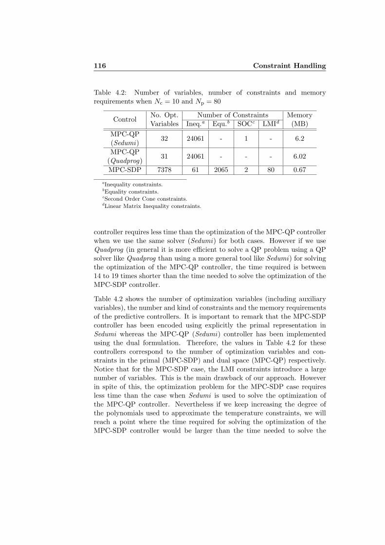
116 Constraint Handling
Table 4.2: Number of variables, number of constraints and memoryrequirements when Nc = 10 and Np = 80
ControlNo. Opt. Number of Constraints MemoryVariables Ineq.a Equ.b SOCc LMId (MB)
MPC-QP32 24061 - 1 - 6.2
(Sedumi)MPC-QP
31 24061 - - - 6.02(Quadprog)MPC-SDP 7378 61 2065 2 80 0.67
aInequality constraints.bEquality constraints.cSecond Order Cone constraints.dLinear Matrix Inequality constraints.
controller requires less time than the optimization of the MPC-QP controllerwhen we use the same solver (Sedumi) for both cases. However if we useQuadprog (in general it is more efficient to solve a QP problem using a QPsolver like Quadprog than using a more general tool like Sedumi) for solvingthe optimization of the MPC-QP controller, the time required is between14 to 19 times shorter than the time needed to solve the optimization of theMPC-SDP controller.
Table 4.2 shows the number of optimization variables (including auxiliaryvariables), the number and kind of constraints and the memory requirementsof the predictive controllers. It is important to remark that the MPC-SDPcontroller has been encoded using explicitly the primal representation inSedumi whereas the MPC-QP (Sedumi) controller has been implementedusing the dual formulation. Therefore, the values in Table 4.2 for thesecontrollers correspond to the number of optimization variables and con-straints in the primal (MPC-SDP) and dual space (MPC-QP) respectively.Notice that for the MPC-SDP case, the LMI constraints introduce a largenumber of variables. This is the main drawback of our approach. Howeverin spite of this, the optimization problem for the MPC-SDP case requiresless time than the case when Sedumi is used to solve the optimization ofthe MPC-QP controller. Nevertheless if we keep increasing the degree ofthe polynomials used to approximate the temperature constraints, we willreach a point where the time required for solving the optimization of theMPC-SDP controller would be larger than the time needed to solve the

4.4 Greedy selection algorithm 117
optimization of MPC-QP with Sedumi.
Finally, from Table 4.2 we can see that the memory requirements (thememory needed to store the matrices that are given to the solver) of theMPC-SDP controller are significantly less than the memory demands ofthe MPC-QP controller (it does not matter the solver used). The MPC-SDP controller requires approximately 9 times less memory than the MPC-QP controller. Although our approach has not led to a reduction in thecomputational time (when the optimization of MPC-QP is performed withQuadprog), it certainly has led to a remarkable saving of memory.
4.4 Greedy selection algorithm
It has been observed that the coefficients of consecutive temperatureconstraints are quite similar. This is a consequence of the fact that the mostrelevant columns of ΦT ∈ R
N×n (the part of the POD basis vectors that isassociated to the temperature profile) are smooth (they do not oscillate toomuch). By taking into account these observations, we propose an algorithmfor selecting a reduced set of constraints from the full set. The output ofthe algorithm would be a matrix ΦR ∈ R
sc×n and a vector TR ∈ Rsc which
define the new set of temperature constraints,
ΦRa(k) ≤ TR. (4.11)
Here Sc is the number of selected constraints and n is the order of the PODmodel.
In this section we are going to adopt a different notation than the one usedin the previous section in order to properly describe the algorithm. Thisnotation is as follows:
• The ith row of the matrix ΦT and the ith entry of the vector TΔmax
are denoted by ΦT(i, :) and TΔmax(i) respectively,
• The entry of the matrix ΦT that lies in the ith row and the jth columnis written as ΦT(i, j),
• ΦR = [ΦR; ΦT(i, :)] indicates that ith row of ΦT is added at thebottom of the matrix ΦR, and TR = [TR; TΔmax(i)] denotes that theith entry of the vector TΔmax is added at the bottom of the vector TR.

118 Constraint Handling
FeasibleRegion
c1c2
c3
FeasibleRegion
c1
c3
If the difference between c1and c2 is small
then, we can drop c2
Original Problem
Cd
Figure 4.12: Operation 1 - Dropping a constraint of a 2nd order PODmodel. Here c1, c2 and c3 are temperature constraints defined as follows.c1 : ΦT(1, 1)a1(k) + ΦT(1, 2)a2(k) ≤ TΔmax(1), c2 : ΦT(2, 1)a1(k) +ΦT(2, 2)a2(k) ≤ TΔmax(2), and c3 : ΦT(3, 1)a1(k) + ΦT(3, 2)a2(k) ≤TΔmax(3).
FeasibleRegion
c1
c3
FeasibleRegion
c1
c3
max3 T 1 T 2: (3,1) ( ) (3, 2) ( ) (3)c a k a k T
max3 T 1 T 2: (3,1) ( ) (3,2) ( ) (3)c a k a k T
c1
FeasibleRegion
c3
Drawback: this region is not included
It is smaller
Figure 4.13: Operation 2 - Reducing the area that does not belong to theoriginal feasible region after dropping a constraint.

4.4 Greedy selection algorithm 119
The main ideas of the proposed algorithm can be explained as follows. Letus suppose that a 2nd order POD model has only 3 temperature constraints,
c1 : ΦT(1, 1)a1(k) + ΦT(1, 2)a2(k) ≤ TΔmax(1)
c2 : ΦT(2, 1)a1(k) + ΦT(2, 2)a2(k) ≤ TΔmax(2)
c3 : ΦT(3, 1)a1(k) + ΦT(3, 2)a2(k) ≤ TΔmax(3)
delimiting the feasible region shown in Figure 4.12. Furthermore, let usdefine the following measure of distance
dC(p, i) =1
n + 1
⎛⎝ n∑
j=1
|ΦT(p, j) − ΦT(i, j)| + |TΔmax(p) − TΔmax(i)|⎞⎠
(4.12)for determining how far or how close two constraints are. Here n is thenumber of POD coefficients or the order of the POD model. The distancedC(p, i) is nothing else than the mean absolute error between the coefficientsof the constraints that are being compared, in this case the pth and ithconstraints.
In the selection algorithm we can distinguish two operations, namely, thedropping of a constraint and the reduction of the feasible region afterdropping a constraint. These operations are illustrated in Figures 4.12and 4.13 respectively. In Figure 4.12 we compare c1 and c2, and then wedrop c2 given that the distance dC(1, 2) between c1 and c2 is smaller thana predefined value. Notice that the new feasible region delimited by thereduced set of constraints c1 and c3, contains a small area (dark gray area inthe figure) that was not part of the feasible region of the original problem.So, in order to reduce the size of this dark gray region, we introduce the so-called shrinking parameter γ to tighten nonconsecutive constraints leadingto a reduction of the feasible region as it is depicted in Figure 4.13. Althoughwe can reduce the size of this dark gray area or even get rid of it by selectinga γ large enough, the drawback of this measure is that we would remove partof the original feasible region. This is of course a conservative measure.
Our greedy selection algorithm is as follows:
1. Set p = 1, and select the first constraint: TR = TΔmax(1), ΦR =ΦT(1, :).
2. For all i = 2, . . . , N − 1, perform:
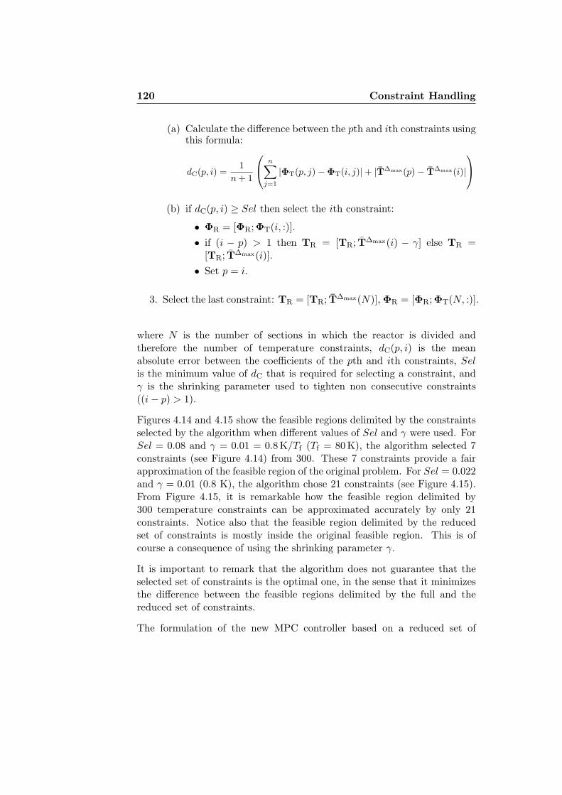
120 Constraint Handling
(a) Calculate the difference between the pth and ith constraints usingthis formula:
dC(p, i) =1
n + 1
⎛⎝ n∑
j=1
|ΦT(p, j) − ΦT(i, j)| + |TΔmax(p) − TΔmax(i)|⎞⎠
(b) if dC(p, i) ≥ Sel then select the ith constraint:
• ΦR = [ΦR; ΦT(i, :)].• if (i − p) > 1 then TR = [TR; TΔmax(i) − γ] else TR =
[TR; TΔmax(i)].• Set p = i.
3. Select the last constraint: TR = [TR; TΔmax(N)], ΦR = [ΦR; ΦT(N, :)].
where N is the number of sections in which the reactor is divided andtherefore the number of temperature constraints, dC(p, i) is the meanabsolute error between the coefficients of the pth and ith constraints, Selis the minimum value of dC that is required for selecting a constraint, andγ is the shrinking parameter used to tighten non consecutive constraints((i − p) > 1).
Figures 4.14 and 4.15 show the feasible regions delimited by the constraintsselected by the algorithm when different values of Sel and γ were used. ForSel = 0.08 and γ = 0.01 = 0.8 K/Tf (Tf = 80 K), the algorithm selected 7constraints (see Figure 4.14) from 300. These 7 constraints provide a fairapproximation of the feasible region of the original problem. For Sel = 0.022and γ = 0.01 (0.8 K), the algorithm chose 21 constraints (see Figure 4.15).From Figure 4.15, it is remarkable how the feasible region delimited by300 temperature constraints can be approximated accurately by only 21constraints. Notice also that the feasible region delimited by the reducedset of constraints is mostly inside the original feasible region. This is ofcourse a consequence of using the shrinking parameter γ.
It is important to remark that the algorithm does not guarantee that theselected set of constraints is the optimal one, in the sense that it minimizesthe difference between the feasible regions delimited by the full and thereduced set of constraints.
The formulation of the new MPC controller based on a reduced set of

4.4 Greedy selection algorithm 121
0 20 40 60
−20
0
20
40
60
−5 0 5 10 15
−10
0
10
20 zoom in
feasible regionfeasible region
a1(k)a1(k)
a2(k
)
a2(k
)
Figure 4.14: Feasible region delimited by the temperature constraints of a2nd order POD model. Dashed line - Full set of constraints. Solid line - 7constraints selected by the algorithm when Sel = 0.08 and γ = 0.01 (0.8 K).
0 20 40 60
−20
0
20
40
60
−5 0 5 10 15
−10
0
10
20 zoom in
feasible regionfeasible region
a1(k)a1(k)
a2(k
)
a2(k
)
Figure 4.15: Feasible region delimited by the temperature constraints of a2nd order POD model. Dashed line - Full set of constraints. Solid line - 21constraints selected by the algorithm when Sel = 0.022 and γ = 0.01 (0.8K).
temperature constraints is given by
minaNp ,ΔuNc ,dNp ,ξ
Np∑i=1
‖aref(k + i) − a(k + i)‖2Q+
Nc−1∑i=0
‖Δu(k + i)‖2R+ (4.13a)
+PQξ2 + PLξ
subject to
a(k + i + 1) = Aa(k + i) + Bu(k + i) + Fd(k + i), i = 0, . . . , Np − 1,
d(k + i + 1) = d(k + i), i = 0, . . . , Np − 1,

122 Constraint Handling
u(k + i) = u(k + i − 1) + Δu(k + i), i = 0, . . . , Nc − 1,
u(k + i) = u(k + i − 1), i = Nc, . . . , Np − 1,
umin ≤ u(k + i) ≤ umax, i = 0, . . . , Nc − 1,
ΦRa(k + i) ≤ TR + 1 · η(i)ξ, i = 1, . . . , Np, (4.13b)ξ ≥ 0,
with
aNp = [a(k + 1); a(k + 2); . . . ; a(k + Np)]dNp = [d(k + 1); d(k + 2); . . . ; d(k + Np)]
ΔuNc = [Δu(k); Δu(k + 1); . . . ; Δu(k + Nc − 1)]
η(i) = 1/ri−1c , rc > 1.
Observe that the only difference of this formulation and the one of theMPC-QP controller described by (4.1), is the definition of the temperatureconstraints, where ΦT and TΔmax have been substituted by ΦR and TR in(4.1b), and the vector of 1’s has been properly resized. From now on, thisnew MPC with a reduced set of temperature constraints will be referred toas MPC-QP-RS.
The MPC-QP-RS controller has the same tuning parameters as the MPC-QP controller presented in Section 4.2, and it uses the same Kalman filter(3.17) as described in Section 3.4.1. For this controller we have set Sel = 0.03and γ = 0.00625 (0.5 K) in the algorithm, and it has selected Sc = 20constraints.
Unlike the MPC-QP which deals with 24 000 temperature constraints, thisMPC has only Sc×Np = 20×80 = 1600 constraints. Hence, a large reductionin the number of temperature constraints has been achieved thanks to thegreedy selection algorithm proposed in this section. As it is presented inTable 4.3, this reduction leads to a big saving of memory, since the reducedset of constraints (0.42 MB) require 14.33 times less memory than thecomplete set (6.02 MB).
Finally, observe that the selection algorithm proposed in this section, allowsus to find a suitable set of points where we can impose the temperatureconstraint in the MPC-PV controller (its formulation is in terms of physicalvariables) described by (3.18) when γ = 0. Keep in mind that each selectedrow of ΦT and TΔmax is associated to a specific point of the spatial domain ofthe reactor. Now, if we want to include the effect of the shrinking parameter

4.4 Greedy selection algorithm 123
(γ > 0) in the formulation of MPC-PV and reduce the number of slackvariables, the following modifications should be done:
• In the cost function (3.18a) the term ξTPQξ+PTLξ should be replaced
by PQξ2 + PLξ, where PQ and PL are weighting factors (PQ > 0, PL >0) and ξ is the slack variable (scalar quantity) that accounts for themaximum violation of the temperature constraint along the reactorand the prediction horizon.
• The set of inequality temperature constraints (3.18b) should besubstituted by ΦRa(k + i) ≤ TR + 1 · η(i)ξ, ∀i = 1, . . . , Np.
• The inequality (3.18c) should be replaced by ξ ≥ 0.
4.4.1 Simulation results
For the same reasons discussed in Section 4.3.4, the behavior of MPC-QP-RSwas quite similar to those of the MPC-NTC (see Section 3.5) and MPC-QPcontrollers during Tests 1 and 2. Similarly, we use Test 3 to assess the abilityof the MPC-QP-RS controller of handling the temperature constraint of thereactor. In this section the optimization problem of the MPC controllersis solved by means of Quadprog and they have been implemented using thecondensed form of the MPC formulations presented previously. Figures 4.16,4.17, 4.18, 4.19 and 4.20 show the simulation results during this test.
As it was the case for the MPC-SDP controller in Section 4.3.4, the steadystate profiles of the reactor when the MPC-QP-RS is used, overlap withthe profiles obtained with the MPC-QP and MPC-NTC controllers. Thiscan be observed in Figure 4.16. In Figure 4.17 we can see the evolutionin time of the temperature and concentration at the reactor outlet. Noticethat the differences between the MPC-QP-RS and MPC-QP controllers aremuch smaller than the ones observed between MPC-SDP and MPC-QP (seeFigure 4.4). From here it is clear that the full set of temperature constraintsof MPC-QP is better approximated in the MPC-QP-RS case than in theMPC-SDP case.
In Figure 4.18 we can see the plot of the maximal peak of the temperatureprofile (hot spot), and in Figure 4.19 the plot of its position along Test 3. Asit was pointed out in Section 4.3.4, for the case of the MPC-NTC controllerthe temperature constraint is temporary violated. This is not the case

124 Constraint Handling
0 0.2 0.4 0.6 0.8 1320
340
360
380
400
0 0.2 0.4 0.6 0.8 10
0.005
0.01
0.015
0.02
0.025
Tem
per
atu
re[K
]C
once
ntr
ati
on
[mol/
l]
Length z [m]
Length z [m]
Figure 4.16: Steady-state temperature and concentration profiles of thereactor for Test 3. Dotted line - Nominal profile (reference). Solid line -MPC-QP. Dashed line - MPC-QP-RS. Dash-dotted line - MPC-NTC.
0 5 10 15 20 25 30 35345
350
355
360
0 5 10 15 20 25 30 350
1
2
3
4
5x 10
−3
Tem
per
atu
re[K
]C
once
ntr
ati
on
[mol/
l]
t [s]
t [s]
Figure 4.17: Temperature and concentration at the reactor outlet duringTest 3. Solid line - MPC-QP. Dashed line - MPC-QP-RS. Dash-dotted line- MPC-NTC.

4.4 Greedy selection algorithm 125
0 5 10 15 20 25 30 35370
375
380
385
390
395
400
405
410
constraint
t = 1.2 s
Tem
per
atu
re[K
]
t [s]
Figure 4.18: Maximal peak of the temperature profile during Test 3. Solidline - MPC-QP. Dashed line - MPC-QP-RS. Dash-dotted line - MPC-NTC.
0 7 14 21 28 350.1
0.21
0.32
0.43
0.54
0.65MPC−QP
0 7 14 21 28 350.1
0.21
0.32
0.43
0.54
0.65MPC−QP−RS
0 7 14 21 28 350.1
0.15
0.2
0.25
0.3
0.35
0.4
0.45
0.5MPC−NTC
Posi
tion
[m]
Posi
tion
[m]
Posi
tion
[m]
t [s]t [s]t [s]
Figure 4.19: Position of the hot spot (maximal peak of the temperatureprofile) of the reactor during Test 3.

126 Constraint Handling
0 7 14 21 28 35260
280
300
320
340
360
380
400
0 7 14 21 28 35280
300
320
340
360
380
400
420
0 7 14 21 28 35310
315
320
325
330
335
340
constraint
constraint
TJ1 TJ2 TJ3
t [s]t [s]t [s]
Tem
per
atu
re[K
]
Tem
per
atu
re[K
]
Tem
per
atu
re[K
]
Figure 4.20: Control actions (jackets temperatures) of the MPC controllersalong Test 3. Solid line - MPC-QP. Dashed line - MPC-QP-RS. Dash-dottedline - MPC-NTC.
for the MPC-QP and MPC-QP-RS controller that keep the temperatureprofile below 400 K. Notice also, that it is hard to see any difference in theirresponses.
Concerning the control actions of the MPC controllers, which are displayedin Figure 4.20, they are all the time within the allowed limits.
Figure 4.21 shows the controllers’ predictions of the maximal peak of thetemperature profile at t = 1.2 s. From Figure 4.21 it is evident that thetemperature constraints of MPC-QP and MPC-QP-RS are active. Bothcontrollers keep the temperature below and on 400 K along the predictionhorizon, and the difference between their predictions are practically negligi-ble. Note, however, that the predictions of the MPC-QP-RS controller areslightly under the predictions of MPC-QP. This is the effect of the use ofthe shrinking parameter γ in the greedy selection algorithm.
Table 4.3 presents the number of optimization variables, the number oflinear inequality constraints and the memory requirements of the predictivecontrollers. In addition, this table shows the average computation times (ona PC with an Intel Dual Core of 3 Ghz and a RAM memory of 2 GB) for

4.4 Greedy selection algorithm 127
1.2 3.2 5.2 7.2 9.2 11.2 13.2 15.2 17.2385
390
395
400
405
410
415
constraint
t [s] - Prediction horizon (80 samples)
Tem
per
atu
re[K
]
Figure 4.21: Predictions of the maximal peak of the temperature profile att = 1.2 s. Solid line - MPC-QP. Dashed line - MPC-QP-RS. Dash-dottedline - MPC-NTC.
Table 4.3: Number of variables, number of constraints and average time forsolving the optimization problem
ControlNo. Opt. No. inequality Memory
toptVariables constraints (MB)
MPC-QP 31 24061 6.02 0.31 s
MPC-QP-RS 31 1661 0.42 0.023 s
topt = Average time for solving the optimization problem.
QP solver = Quadprog.
solving the optimization problems of the MPC controllers during Test 3.These average times were 0.31 s and 0.023 s for the MPC-QP and MPC-QP-RS cases respectively. The MPC-QP-RS controller requires 13.48 times lesstime than the MPC-QP controller for solving the optimization. To sum up,the reduction in the number of temperature constraints by means of thealgorithm proposed in this section, has not only conduced to a considerable

128 Constraint Handling
saving of memory, but also it has led to a remarkable reduction in thecomputational effort.
4.5 Conclusions
First of all in this chapter we have presented an extension of the MPC-NTCcontroller proposed in Section 3.4, which takes into account the temperatureconstraint of the reactor. We have shown that this extension has to handle avery large number of temperature constraints which demands a considerableamount of memory and computational power. In this chapter we haveproposed two methods to tackle this problem.
In the first method, part of the basis vectors derived with the PODtechnique are approximated with univariate real polynomials. Afterwards,the theory of positive polynomials is used for approximating the temperatureconstraints by means of Linear Matrix Inequalities and linear equalityconstraints. The method leads to a significant reduction in the number ofconstraints which conduces to a considerable saving of the memory. Howeverthe computational time needed for solving the optimization problem of thepredictive controller based on the polynomial approximations, is much largerthan the time required for solving the original problem. What mainly limitsthe computational gain of this technique is the large number of variablesthat are introduced by the LMI constraints. From this study it is clear thatwith this positive polynomial approach the resulting optimization problem ismore complex than the original one. Nevertheless this approach guaranteesthe fulfillment of the temperature constraint at every point of the reactor.
The predictive controller based on the polynomial approximation presenteda good behavior, and it was able to deal with the temperature constraintsquite well.
This approach, that we only applied to linear system models so far, canin a straightforward way be generalized to the case of nonlinear MPC andwould then lead to the interesting problem class of nonlinear SDP problemsthat can, e.g., be addressed by the sequential SDP methods proposed andinvestigated in [42,50,55].
In the second method, we exploit the fact that the coefficients of consecutiveconstraints are quite similar in order to select a reduced set of constraints

4.5 Conclusions 129
from the complete set. This method leads to a significant reduction in thenumber of constraints, which conduces to a considerable saving of memory,and a substantial reduction in the computational time required for solvingthe optimization of the MPC controller. Note however that unlike thepositive polynomial approach, in this method we do not have any commandon the temperature between the discretization points.
The predictive controller based on the reduced set of constraints presented agood behavior and it was able to deal with the temperature constraints quitewell. Additionally, its behavior was practically identical to the behavior ofthe predictive controller based on the complete set of constraints.
Future research is necessary in order to find out which of the techniquesproposed works best for which kind of applications.

130 Constraint Handling

Chapter 5
Performance Improvement inModel Simulation
5.1 Introduction
Several studies have reported that we can get a large model-order reductionby using POD and Galerkin projection. Nevertheless the computation savingoffered by the reduced order models is small when nonlinear or Linear TimeVariant (LTV) systems are considered. The reason of this limitation lies inthe fact that we need the full spatial information from the original high-dimensional systems in order to evaluate the reduced-order models.
In [10–12] a method known as Missing Point Estimation (MPE) is proposedfor tackling this problem. In this method the Galerkin projection isconducted only on some pre-selected state variables instead of the entireset. The remaining state variables are estimated by means of the PODbasis vectors. It has been reported that this technique can save considerablecomputational effort.
In this chapter we present two alternative techniques for accelerating theevaluation of nonlinear POD models.
In the first method a Multi-Layer Perceptron (MLP) neural network is usedto approximate the nonlinear vector function of the POD models [7]. Giventhat the time for evaluating the trained MLP can be very short, we canobtain a significant saving of computational time.
131
132 Performance Improvement in Model Simulation
The second method is mainly intended for accelerating nonlinear PODmodels derived from input-affine high-dimensional systems with polynomialnonlinearities [6]. It turns out that by exploiting their polynomial nature, wecan construct compact and efficient representations that can be evaluatedmuch faster. Besides, the computational gain can be increased even more,if we use sequential feature selection algorithms for choosing the mostrelevant monomials (suboptimal solution) of these representations. Noticethat this approach might also be applied to high-dimensional systems withnon-polynomial nonlinearities, provided that these nonlinearities can beapproximated by low degree polynomials.
Usually, the model reduction of a stable model by POD often results in areduced order model that is stable as well. However, this is generally notguaranteed [119]. By using Lyapunov’s indirect method we can obtain aneigenvalue constraint that can be used for guaranteeing the local stability ofa POD model with polynomial nonlinearities. Since this constraint leadsto a non-smooth optimization problem, which is difficult to solve in itsoriginal form, in this chapter we also present two manners of dealing with thisconstraint. In both cases, the local stability is guaranteed independently ofthe data used, although the quality of the reduced-order model still dependson the quality of the data.
This chapter is organized as follows. Section 5.2 presents a descriptionof the dynamical system that will be used to explain our techniques, thenonlinear heat transfer problem in a one-dimensional bar. In Section 5.3the derivation of a reduced order model for the bar by means of PODand Galerkin projection is discussed. Section 5.4 explains our approachfor speeding up nonlinear POD models by using neural networks. In Section5.5 we introduce our technique for accelerating the nonlinear POD modelfound in Section 5.3 by exploiting its polynomial nature. Section 5.6 discusshow the local stability of POD models with polynomial nonlinearities canbe guaranteed. In Section 5.7 we present some validation and simulationresults. Finally Section 5.8 presents some concluding remarks.

5.2 Nonlinear heat transfer in a one-dimensional bar 133
5.2 Nonlinear heat transfer in a one-dimensionalbar
The system under study is the silicon bar shown in Figure 5.1. The barhas attached an actuator which provides a uniformly distributed heat fluxu(t) between z = za and z = zb. Additionally, an external heat flux d(t)is applied uniformly along the bar whose ends are kept at 25◦C (ambienttemperature) all the time.
If only temperature variations in the z-direction are considered, thedynamics of the temperature T (z, t) of the bar can be modeled by thefollowing nonlinear PDE:
ρCp∂T (z, t)
∂t=
∂
∂z
(κ (T (z, t))
∂T (z, t)∂z
)+ V (z, t) (5.1)
with the following initial and boundary conditions:
T (z, t = 0) = 25◦CT (z = 0, t) = T (z = L, t) = 25◦C.
Here ρ is the material density in [kg · m−3], Cp is the heat capacity in[J · kg−1 · K−1], κ (T ) is the temperature dependent heat conductivity in[J · s−1 · m−1 · K−1], t is the time in [s], z is the spatial coordinate in [m]and V (z, t) is the heat source applied to the bar at position z and time t in[W · m−3]. V (z, t) is defined as follows:
V (z, t) ={
d(t) + u(t), za ≤ z ≤ zb
d(t), elsewhere.
The relation between the temperature and the heat conductivity κ (T ) isdescribed by a polynomial of degree 3,
κ(T ) = κ0 + κ1T + κ2T2 + κ3T
3 (5.2)
where κ0 = 36, κ1 = −0.1116, κ2 = 1.7298×10⁻⁴ and κ3 = −1.78746×10⁻⁷
are real coefficients in the appropriated units.
The length of the bar is L = 0.1 m and the remaining numerical values ofthe model parameters are: ρ = 3970 kg · m−3, Cp = 766 J · kg−1 · K−1,za = 0.005 m and zb = 0.04 m.

134 Performance Improvement in Model Simulation
The operating ranges in [W · m−3] of d(t) and u(t) are −500 · 103 ≤ d(t) ≤500 · 103 and −1500 · 103 ≤ u(t) ≤ 1500 · 103 respectively. Some of theprevious numerical values were inspired on the values given in [156].
For simulation purposes, it is necessary to reduce the infinite dimensionalityof (5.1) by discretizing the spatial domain. To this end, the partialderivatives with respect to space were replaced by backward (the innerspatial derivative) and forward (the outer spatial derivative) differenceapproximations. This is equivalent to replace the second partial derivativewith respect to space by a central difference approximation in the linearversion of the heat equation where κ is kept constant (see for example (2.23)and (2.25)). The discretized model of the bar is given by the following setof nonlinear ordinary differential equations:
dTi
dt= c1
(κ(Ti+1)Ti+1 −
(κ(Ti+1) + κ(Ti)
)Ti + κ(Ti)Ti−1
)+ c2Vi (5.3a)
for i = 1, . . . , N − 1,
with
c1 =1
ρCp (Δz)2(5.3b)
c2 =1
ρCp
T0 = TN = 25◦C
where N is the number of sections in which the bar is divided, Δz is thelength of each section, and Ti and Vi are the temperature and heat flux atthe point zi = iΔz.
If we define T(t) ∈ RN−1 = [T1(t), T2(t), . . . , TN−1(t)]T as the vector
containing the temperature of the grid points from z1 till zN−1 every timeinstant, we can write Equation (5.3) as follows:
T(t) = F (T(t)) + B1d(t) + B2u(t) (5.4)
where F (T(t)) : RN−1 → R
N−1 is a vector-valued or vector function whichcontains the nonlinear terms of the model and whose ith component functionis given by
Fi(T(t)) = c1
(κ(Ti+1(t))Ti+1(t) − (κ(Ti+1(t)) + κ(Ti(t))
)Ti(t)+
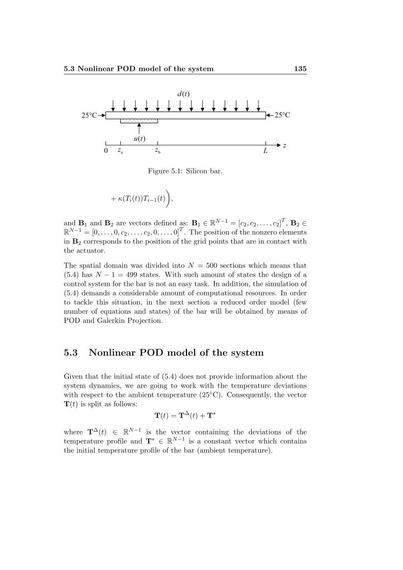
5.3 Nonlinear POD model of the system 135
( )u t
25 C
( )d t
0 az bz Lz
25 C
Figure 5.1: Silicon bar.
+ κ(Ti(t))Ti−1(t))
,
and B1 and B2 are vectors defined as: B1 ∈ RN−1 = [c2, c2, . . . , c2]T , B2 ∈
RN−1 = [0, . . . , 0, c2, . . . , c2, 0, . . . , 0]T . The position of the nonzero elements
in B2 corresponds to the position of the grid points that are in contact withthe actuator.
The spatial domain was divided into N = 500 sections which means that(5.4) has N − 1 = 499 states. With such amount of states the design of acontrol system for the bar is not an easy task. In addition, the simulation of(5.4) demands a considerable amount of computational resources. In orderto tackle this situation, in the next section a reduced order model (fewnumber of equations and states) of the bar will be obtained by means ofPOD and Galerkin Projection.
5.3 Nonlinear POD model of the system
Given that the initial state of (5.4) does not provide information about thesystem dynamics, we are going to work with the temperature deviationswith respect to the ambient temperature (25◦C). Consequently, the vectorT(t) is split as follows:
T(t) = TΔ(t) + T∗
where TΔ(t) ∈ RN−1 is the vector containing the deviations of the
temperature profile and T∗ ∈ RN−1 is a constant vector which contains
the initial temperature profile of the bar (ambient temperature).

136 Performance Improvement in Model Simulation
0 500 1000 1500 2000−5
−2.5
0
2.5
5x 10
6
0 500 1000 1500 2000−2
−1
0
1
2x 10
6
u(t
)d(t
)
t [s]
t [s]
Figure 5.2: Pseudo random multilevel noise signals used in the generationof the snapshot matrix Tsnap. Amplitudes in [W · m−3].
Similarly as it was done in Sections 2.4.3 and 3.3, the reduced order modelof (5.4) is derived in four steps as follows:
1. Generation of the Snapshot Matrix. The snapshot matrixTsnap ∈ R
499×2001 has been built by collecting the evolution of thedeviations of the temperature profile when Pseudo Random MultilevelNoise Signals (PRMNS) were applied to the process inputs u(t) andd(t),
Tsnap =[TΔ(t = 0),TΔ(t = Δt), . . . ,TΔ (t = (Nd − 1)Δt)
]. (5.5)
Here, Nd = 2001 is the number of samples gathered using a samplingtime Δt of 1 s. The excitation signals can be observed in Figure5.2. A commutation probability of 3% was set for the signals and theamplitudes in [W ·m−3] of d(t) and u(t) were restricted to the intervals[−500 · 103, 500 · 103] and [−1500 · 103, 1500 · 103] respectively.
2. Derivation of the POD basis vectors. We have found the PODbasis vectors Φ ∈ R
499×499 = [ϕ1,ϕ2, . . . ,ϕ499] by performing theSVD (the POD basis vectors are the left singular vectors) of the

5.3 Nonlinear POD model of the system 137
0 10 20 30 40 5010
−16
10−14
10−12
10−10
10−8
10−6
10−4
10−2
1−
Pn
n
Figure 5.3: The logarithmic plot of 1 − Pn which is used to determine thetruncation degree of the POD basis vectors.
snapshot matrix Tsnap,
Tsnap = ΦΣΨT
where Φ ∈ R499×499 and Ψ ∈ R
2001×2001 are unitary matrices andΣ ∈ R
499×2001 is a matrix containing the singular values in its maindiagonal.
3. Selection of the most relevant POD basis vectors. We havechosen the n most relevant POD basis vectors based on the energycriterion discussed in Section 2.2.1. Figure 5.3 shows the plot of 1− Pn
(see Equation (2.7)) for the first 50 basis vectors. For this problemwe have selected the first n = 6 POD basis vectors based on theirtruncation degree 1− Pn = 3.194 ·10−7. The selected basis vectors canbe observed in Figure 5.4.
The 6th order approximation of TΔ(t) is then given by
TΔn (t) =
6∑j=1
aj(t)ϕj = Φna(t) (5.6)
where Φn = [ϕ1,ϕ2, . . . ,ϕ6] and a(t) = [a1(t), a2(t), . . . , a6(t)]T .

138 Performance Improvement in Model Simulation
0 0.02 0.04 0.06 0.08 0.1−0.08
−0.06
−0.04
−0.02
0
0 0.02 0.04 0.06 0.08 0.1−0.08
−0.005
0.07
0 0.02 0.04 0.06 0.08 0.1−0.08
0
0.08
0 0.02 0.04 0.06 0.08 0.1−0.1
−0.01
0.08
0 0.02 0.04 0.06 0.08 0.1−0.1
−0.015
0.07
0 0.02 0.04 0.06 0.08 0.1−0.12
−0.02
0.08
ϕ1 ϕ2
ϕ3 ϕ4
ϕ5 ϕ6
z [m]z [m]
Figure 5.4: Selected POD basis vectors.
4. Construction of the model for the first n=6 POD coefficients.The dynamic model for the POD coefficients is derived by performingthe Galerkin projection of the nonlinear model (5.4) on the spacespanned by the selected basis vectors Φn = [ϕ1,ϕ2, . . . ,ϕ6]. Thus,if we replace T(t) by its nth order approximation Tn(t) = TΔ
n +T∗ =Φna(t)+T∗ in Equation (5.4), and we apply the inner product criterionto the resulting equation, we have that⟨
Φna(t),ϕj
⟩=⟨F (Φna(t) + T∗) + B1d(t) + B2u(t),ϕj
⟩, (5.7)
∀j = 1, 2, . . . , n = 6.
By evaluating the inner product in (5.7),
ΦTnΦna(t) = ΦT
nF (Φna(t) + T∗) + ΦTnB1d(t) + ΦT
nB2u(t)
a(t) = ΦTnF (Φna(t) + T∗) + ΦT
nB1d(t) + ΦTnB2u(t) (5.8)

5.4 Acceleration of POD models by using neural networks 139
we get the model for the first n = 6 POD coefficients. Hence, thereduced order model of the bar with only 6 states is given by,
a(t) = ΦTnF (Φna(t) + T∗) + B1d(t) + B2u(t) (5.9)
Tn(t) = Φna(t) + T∗
where B1 = ΦTnB1 and B2 = ΦT
nB2. Finally if we define a new vector-valued function f : R
6 → R6 as f (a(t)) = ΦT
nF (Φna(t) + T∗), thenthe reduced order model of the bar can be written more compactly asfollows:
a(t) = f (a(t)) + B1d(t) + B2u(t) (5.10a)
Tn(t) = Φna(t) + T∗. (5.10b)
In general, it should be clear that we do not know the compact expressionof f(a(t)) in (5.10a). So, in order to simulate the reduced order model,the ODE solver has to evaluate indirectly f(a(t)). Firstly, the solver hasto map the state of the reduced order model a(t) into the original high-dimensional space by means of this linear transformation TΔ
n (t) = Φna(t).Secondly it has to evaluate the resulting high-dimensional state vector TΔ
n (t)in the vector function F(TΔ
n (t) + T∗) of (5.4), and finally it has to map theresults of this evaluation to the low dimensional space by pre-multiplyingthem by ΦT
n . The evaluation of f(a(t)) is done as many times as it isrequired by the ODE solver within each integration step. Hence the indirectevaluation of f(a(t)) is the bottleneck that limits severely the computationalgain of the nonlinear POD model. In order to overcome this situation, inthe next sections we present two approaches for speeding up the evaluationof nonlinear POD models like (5.10). In the first method we use feedforwardneural networks and in the second one we exploit the polynomial nature ofthese POD models.
5.4 Acceleration of POD models by using neuralnetworks
In order to speed up the evaluation of (5.10a) we propose to approximatethe vector function f : R
6 → R6 by using a multi-layer perceptron neural
network. In this way we eliminate the necessity of evaluating the vector
140 Performance Improvement in Model Simulation
function F : R499 → R
499 of the full order model and we can save aconsiderable amount of time.
As it is well-known, a multi-layer perceptron can learn any nonlinear input-output mapping given an adequate number of hidden neurons (each onewith a nonlinear activation function) in its hidden layers [63]. In addition,the time required for calculating the MLP output can be quite short sinceonly few matrix multiplications, vector additions and function evaluationsare necessary. Due to these characteristics, an MLP is a suitable choice forapproximating the vector function f in (5.10a).
In order to generate the input and output data required for training,validating and testing the MLP, firstly the POD model (5.10) was excitedwith PRMNS signals and the evolution of the state vector a(t) was collected.From the test the following data sets were constructed:
U = {u(0), u(Δt), . . . , u(10000Δt)} ,
D = {d(0), d(Δt), . . . , d(10000Δt)} ,
A = {a(0),a(Δt), . . . ,a(10000Δt)} .
In the experiment 10001 samples were gathered with a sampling time Δtequal to 1 s. The commutation probability of the PRMNS signals was setto 3% and the amplitudes in [W · m−3] of d(t) and u(t) were restricted tothe intervals [−600 · 103, 600 · 103] and [−1800 · 103, 1800 · 103] respectively.Notice that these intervals are 20% larger than the operating ranges definedin Section 5.2. This enlarges the range of validity of our approximation withthe MLP.
If we define a vector y(t) ∈ R6 as follows:
y(t) = a(t) − B1d(t) − B2u(t), (5.11)
then (5.10a) can be cast as y(t) = f(a(t)). By using (5.10a) and the datasets U ,D and A, we can easily calculate a(t) at each sampling time andafterwards y(t) by means of (5.11). The evolution in time of y(t) is thencompiled in the following data set
Y = {y(0),y(Δt), . . . ,y(10000Δt)} .
In order to make the training of the MLP more efficient, the input data Aand the target outputs Y were normalized for zero mean and unit variance

5.4 Acceleration of POD models by using neural networks 141
hW
hb1
oW
ob1
Hidden Layer Output Layer
nor ( )ta norˆ ( )ty
h ( )g
Input
Figure 5.5: Structure of the multi-layer perceptron. anor(t) ∈ R6 and
ynor(t) ∈ R6
by applying the normalization functions h : R6 → R
6 and v : R6 → R
6
to each element of the datasets A and Y respectively. The ith componentfunction of the vector functions h and v is defined as
anori (t) = hi (a(t)) =
ai(t) − ai
σai
, (5.12)
ynori (t) = vi (y(t)) =
yi(t) − yi
σyi
, (5.13)
where ai, yi and σai , σyi are the mean and the standard deviation of ai(t)and yi(t) in A and Y respectively.
At the moment of using the MLP after training, the input data has to benormalized by using (5.12) and the output of the neural network needs to berestored using the inverse function of (5.13) whose ith component functionis defined as follows:
yi(t) = v−1i (ynor(t)) = ynor
i (t)σyi + yi.
Here the “hat” on top of yi and ynori are used to stress that the output of the
MLP is just an approximation of the target output. The data sets containingthe normalized input data and output targets are denoted as Anor and Ynor
respectively.
The structure of the MLP neural network designed for this problem ispresented in Figure 5.5. The number of inputs and the number of outputneurons is determined by the number of POD coefficients. So, there are 6inputs in the input layer and 6 neurons in the output layer. Regarding the

142 Performance Improvement in Model Simulation
number of hidden layers, the MLP has only one. It has been shown thatmerely one hidden layer suffices for approximating any function given anadequate number of hidden neurons with continuous nonlinear activationfunctions [67]. The output of the MLP is given by the following expression:
ynor(t) = Wo · gh(Wh · anor(t) + bh
)+ bo (5.14)
where Nhn is the number of hidden neurons, Wh ∈ RNhn×n is the matrix
of weights that links the input layer to the hidden layer, the entry W hji of
Wh corresponds to the connection weight from the ith input neuron to thejth neuron in the hidden layer, bh ∈ R
Nhn is the vector containing the biasweight of each neuron of the hidden layer, Wo ∈ R
n×Nhn is the matrix ofweights that links the hidden layer to the output layer, the entry W o
ji ofWo is the connection weight from the ith hidden neuron to the jth neuronin the output layer, bo ∈ R
n is the vector that contains the bias weight ofeach neuron of the output layer, and gh(·) : R
Nhn → RNhn is a vector-valued
function whose component functions are the nonlinear activation functionsof the hidden neurons. The ith component function of gh(·) is a hyperbolictangent function which is defined by the following equation
ghi (sh) =
e2shi − 1
e2shi + 1
,
where sh ∈ RNhn is the vector containing the weighted sum of each hidden
neuron.
The MLP was trained by using the Levenberg-Marquardt (LM) backprop-agation algorithm [62] which is available in the Matlab Neural NetworkToolbox [102]. In general, this algorithm offers a good speed of convergenceand acceptable memory requirements when it is used for approximatingfunctions with networks that contain up to a few hundred weights. In orderto avoid the overfitting of the MLP, the early stopping method was usedduring the training, and therefore the data (Anor and Ynor) was divided into3 sets: the training set with 7001 data points, the validation set with 1500data points and the test set with 1500 data points. The training set is usedby the training algorithm for updating the network weights and biases, thevalidation set is used for detecting the overfitting during the training stageand the test set is used for testing the generalization capabilities of the MLP.The test set is never used during the training stage. The data was divided bycycling samples (interleaved data division) between training set, validation

5.4 Acceleration of POD models by using neural networks 143
0 2 4 6 8 10 12 1410
−8
10−6
10−4
10−2
100
Mea
n sq
uare
d er
ror
Number of hidden neurons
Training setTest set
0 2 4 6 8 10 12 140
50
100
150
200
Number of hidden neurons
Num
ber
of w
eigh
ts
Figure 5.6: Mean squared error and size of the trained MLP in function ofthe number of hidden neurons.
set, and test set according to percentages. These percentages were 70%,15% and 15% for the training, validation and test sets respectively.
Thus far, there is no theory that establishes the number of hidden unitsthat are needed to achieve some prescribed degree of accuracy in a functionapproximation problem. Therefore, in order to find a suitable number ofhidden units, we increased one by one the number of neurons of the hiddenlayer while checking the error in the approximation of the vector functionf . The Mean Squared Error (MSE) function was selected to measure theperformance of the neural network. The top plot of Figure 5.6 shows theMSE between the target outputs and the MLP output in function of thenumber of hidden neurons. Each value shown in the plot corresponds tothe smallest MSE found after 7 training sessions where the weights of thenet were randomly initialized. The bottom plot of Figure 5.6 presents thenumber of weights of the network in function of the number of hidden units.We chose the MLP with Nhn = 10 hidden neurons since it provides a goodtrade-off between the accuracy of the function approximation and the sizeof the network (136 weights), which determines how fast the MLP can beevaluated and therefore the computational gain that can be obtained. The

144 Performance Improvement in Model Simulation
0 250 500 750 1000 1250 1500−4
−2
0
2
4
0 250 500 750 1000 1250 1500−2
−1
0
1
2
y1
y6
samples
samples
Figure 5.7: MLP test performance for the outputs y1(t) and y6(t). Solid line- Data points (targets). Dashed line - MLP.
MSE of this MLP for the training set is 8.0662 × 10⁻⁷ and for the test setis 8.0975 × 10⁻⁷. These errors were achieved after 6000 epochs of training.Figure 5.7 shows the MLP output and the original data points (targets) fory1(t) and y6(t) when the test set is used. The MLP output is practicallyoverlapping the data points, and it is really difficult to see any difference. Itis clear that the network has learned the nonlinear input-output mapping fwith a high degree of accuracy, and additionally the net has shown a goodgeneralization capability. One factor that contributes to have very smallMSE errors is the absence of noise in the data.
Finally, the equation of the POD model where the function f has beenapproximated by an MLP is the following one:
a(t) = f (a(t)) + B1d(t) + B2u(t) (5.15)
Tn(t) = Φna(t) + T∗
withf (a(t)) = v−1
(Wo · gh
(Wh · h (a(t)) + bh
)+ bo
).
From now on, this POD model will be referred to as Neural-POD model.

5.5 Polynomial POD models 145
5.5 Polynomial POD models
In this section we exploit the polynomial nature of the vector function f(a(t))in (5.10a), in order to find an alternative representation of f(a(t)) that canbe evaluated much faster.
We start by noticing that the mth component function of f(a(t)) =ΦT
nF(Tn(t)) can be written as
fm(a(t)) =N−1∑i=1
ϕi,mFi(Tn(t)) (5.16)
where ϕi,m is the ith entry of the basis vector ϕm, N = 500 is the numberof sections in which the bar was divided, n = 6 is the number of selectedbasis vectors, Tn(t) is the nth order approximation of T(t) and Fi is the ithcomponent function of F(Tn(t)) defined as follows:
Fi(Tn(t)) = c1
(κ(Ti+1(t))Ti+1(t) − (κ(Ti+1(t)) + κ(Ti(t))
)Ti(t)+ (5.17)
+ κ(Ti(t))Ti−1(t))
,
where c1 is a constant given by (5.3b), κ(T ) : R → R is the scalar polynomialfunction defined in (5.2) and Ti(t) is the ith entry of the vector Tn(t) thatis given by
Ti(t) =n∑
j=1
ϕi,jaj(t) + T ∗i (5.18)
where ϕi,j is the ith entry of the basis vector ϕj , aj is the jth POD coefficientand T ∗
i is the ith entry of T∗ which contains the initial temperature profileof the bar. If we replace (5.18) in (5.17),
Fi (a(t)) = c1
⎛⎝κ
⎛⎝ n∑
j=1
ϕ(i+1),jaj(t) + T ∗i+1
⎞⎠⎛⎝ n∑
j=1
ϕ(i+1),jaj(t) + T ∗i+1
⎞⎠−
−⎛⎝κ
⎛⎝ n∑
j=1
ϕ(i+1),jaj(t) + T ∗i+1
⎞⎠+ κ
⎛⎝ n∑
j=1
ϕi,jaj(t) + T ∗i
⎞⎠⎞⎠×
×⎛⎝ n∑
j=1
ϕi,jaj(t) + T ∗i
⎞⎠+

146 Performance Improvement in Model Simulation
+κ
⎛⎝ n∑
j=1
ϕi,jaj(t) + T ∗i
⎞⎠⎛⎝ n∑
j=1
ϕ(i−1),jaj(t) + T ∗i−1
⎞⎠⎞⎠ (5.19)
then we obtain the component function Fi in terms of the POD coefficientsaj(t) ∀j = 1, . . . , n associated to the selected basis vectors. Notice that thisfunction is a multivariate polynomial of degree dp = 4 in aj(t) ∀j = 1, . . . , n.Since fm (a(t)) (see (5.16)) is a linear combination of the functions Fi(a(t))∀i = 1, . . . , N−1, fm (a(t)) is also a multivariate polynomial of degree dp = 4in aj(t) ∀j = 1, . . . , n.
After replacing (5.19) in (5.16) and simplifying the resulting expression, weobtain the following general representation for fm(a(t)),
fm(a(t)) = wm,0 + wm,1a1(t) + · · · + wm,nan(t)+ (5.20)
+ wm,(n+1)a21(t) + wm,(n+2)a1(t)a2(t) + · · · + wm,(r−1)a
dpn (t)
where wm,i is the real coefficient of the ith monomial (i = 0, 1, 2, . . . , r−1) ofthe function fm(a(t)), dp is the largest possible degree for each monomial andr is the number of monomials which is given by the following formula [60]:
r =dp∑
j=0
(n + j − 1
j
)=
dp∑j=0
(n + j − 1)!j! (n − 1)!
. (5.21)
For this particular problem, the number of monomials per componentfunction is equal to 210. The monomials (without coefficients) ai1ai2 · · · ais
of degree s (1 ≤ s ≤ dp) in (5.20) are built from the set C,
C ={〈i1, i2, · · · , is〉 : 1 ≤ i1, i2, . . . , is ∈ Z
+ ≤ n, i1 ≤ i2 ≤ · · · ≤ is}
which contains the possible combinations of the indexes i1, i2, . . . , is.
By using the general representation of f(a(t)) defined in (5.20) through itscomponent functions, we can recast the POD model (5.10) as follows:
a(t) = f (a(t)) + B1d(t) + B2u(t) (5.22)
Tn(t) = Φna(t) + T∗
with
f (a(t)) = [f1 (a(t)) , . . . , fm (a(t)) , . . . , fn (a(t))]T
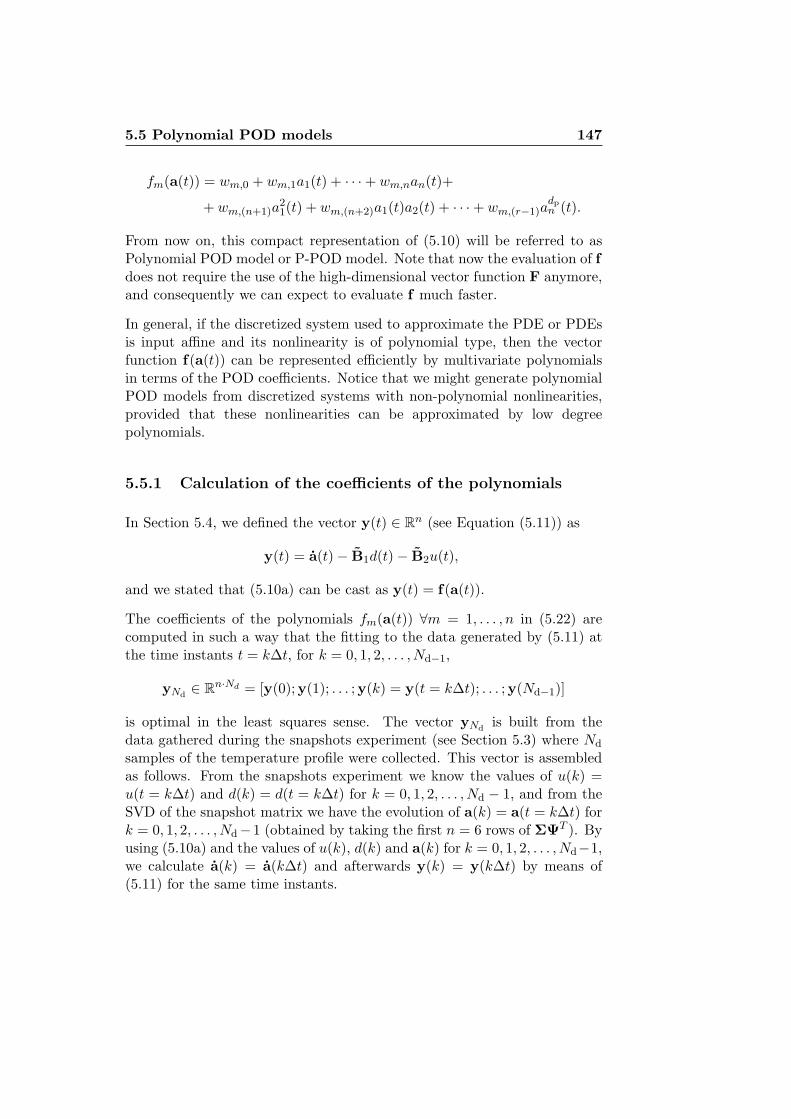
5.5 Polynomial POD models 147
fm(a(t)) = wm,0 + wm,1a1(t) + · · · + wm,nan(t)+
+ wm,(n+1)a21(t) + wm,(n+2)a1(t)a2(t) + · · · + wm,(r−1)a
dpn (t).
From now on, this compact representation of (5.10) will be referred to asPolynomial POD model or P-POD model. Note that now the evaluation of fdoes not require the use of the high-dimensional vector function F anymore,and consequently we can expect to evaluate f much faster.
In general, if the discretized system used to approximate the PDE or PDEsis input affine and its nonlinearity is of polynomial type, then the vectorfunction f(a(t)) can be represented efficiently by multivariate polynomialsin terms of the POD coefficients. Notice that we might generate polynomialPOD models from discretized systems with non-polynomial nonlinearities,provided that these nonlinearities can be approximated by low degreepolynomials.
5.5.1 Calculation of the coefficients of the polynomials
In Section 5.4, we defined the vector y(t) ∈ Rn (see Equation (5.11)) as
y(t) = a(t) − B1d(t) − B2u(t),
and we stated that (5.10a) can be cast as y(t) = f(a(t)).
The coefficients of the polynomials fm(a(t)) ∀m = 1, . . . , n in (5.22) arecomputed in such a way that the fitting to the data generated by (5.11) atthe time instants t = kΔt, for k = 0, 1, 2, . . . , Nd−1,
yNd∈ R
n·Nd = [y(0); y(1); . . . ; y(k) = y(t = kΔt); . . . ; y(Nd−1)]
is optimal in the least squares sense. The vector yNdis built from the
data gathered during the snapshots experiment (see Section 5.3) where Nd
samples of the temperature profile were collected. This vector is assembledas follows. From the snapshots experiment we know the values of u(k) =u(t = kΔt) and d(k) = d(t = kΔt) for k = 0, 1, 2, . . . , Nd − 1, and from theSVD of the snapshot matrix we have the evolution of a(k) = a(t = kΔt) fork = 0, 1, 2, . . . , Nd−1 (obtained by taking the first n = 6 rows of ΣΨT ). Byusing (5.10a) and the values of u(k), d(k) and a(k) for k = 0, 1, 2, . . . , Nd−1,we calculate a(k) = a(kΔt) and afterwards y(k) = y(kΔt) by means of(5.11) for the same time instants.

148 Performance Improvement in Model Simulation
Notice that the mth component function of f(a(t)) defined at the samplingtimes t = kΔt (with k = 0, 1, 2, . . .) can be written as follows:
fm (a(k)) = fm (a(t = kΔt)) = α(k)wm (5.23)
where α(k) ∈ R1×r is a row vector defined as
α(k) =[1, a1(k), a2(k), . . . , an(k), a2
1(k), a1(k)a2(k), . . . ,
a2n(k), . . . , adp
1 (k), adp−11 (k)a2(k), . . . , adp
n (k)],
and wm ∈ Rr
wm =[wm,0, wm,1, wm,2, . . . , wm,(r−1)
]Tis a vector containing the coefficients of the monomials. From here the vectorfunction f(a(k)) = f(a(t = kΔt)) can be compactly formulated in this way
f(a(k)) = Λ(k)w (5.24)
where
Λ(k) ∈ Rn×(r·n) =
⎡⎢⎢⎢⎢⎣α(k) 0 · · · 0
0 α(k). . .
......
. . . . . . 00 · · · 0 α(k)
⎤⎥⎥⎥⎥⎦ ,
andw ∈ R
r·n = [w1; w2; . . . ; wm; . . . ; wn]
is a vector containing all the coefficients that we want to find.
The predictions of (5.24) regarding y(k) for k = 0, 1, 2, . . . , Nd−1, are givenby the following expression
yNd= Ωw (5.25)
where yNd∈ R
n·Nd and Ω ∈ R(n·Nd)×(r·n) are defined as
yNd= [f(a(0)); f(a(1)); . . . ; f(a(k)); . . . ; f(a(Nd − 1))]
Ω = [Λ(0); Λ(1); . . . ; Λ(k); . . . ; Λ(Nd − 1)] .
As it was mentioned before, the coefficients w of the vector function f arefound by means of the least squares method in which the minimizationproblem
minw
J = (yNd− yNd
)T (yNd− yNd
) (5.26)

5.5 Polynomial POD models 149
is solved. We can obtain an equivalent optimization problem in terms of wby substituting (5.25) in (5.26) and ignoring the resulting constant term,
minw
12wT(ΩTΩ
)w − (yT
NdΩ)w. (5.27)
As it is well-known, the solution of this minimization problem can be foundby solving this equation:
(ΩTΩ
)w = ΩTyNd
. In this study this equation issolved by using the QR (orthogonal, triangular) decomposition of ΩTΩ andback substitution. This procedure is numerically more stable than invertingthe matrix product ΩTΩ.
Finally, it is important to remark that in the calculation of the monomialcoefficients the data (a(k), y(k), for k = 0, 1, 2, . . . , Nd − 1) was normalizedfirst (by dividing by the standard deviation) in order to avoid numericalproblems. Consequently, at the moment of evaluating the derivative of theP-POD model we have to carry out the appropriated conversions. For thesake of clarity and simplicity in our derivations, we did not include thenormalization part in the previous equations.
5.5.2 Reduction of the number of monomials
From (5.21) it is clear that the number of monomials of the P-POD modelcan be very large. In fact, this number increases exponentially with thenumber of POD coefficients, compromising the computational gain of theP-POD model. We can tackle this situation by properly selecting a reducedset of monomials whose combination provides a good approximation of thevector function f(a(t)). To this end, in this section we propose the use ofthe sequential feature selection methods [61, 81, 105, 152]. Here we will usethe term “features” for referring to as the “monomials” of f (a(t)).
Sequential feature selection methods have basically two components: theobjective function, called the criterion, which the method seeks to minimizeover all feasible feature subsets, and the sequential search algorithm. Thealgorithm adds or removes features from a candidate subset while evaluatingthe criterion. In general, an exhaustive evaluation of all possible featuresubsets is infeasible, since we have to deal with 2r = 2210 = 1.64 × 1063
candidates. This is why a suboptimal search strategy is necessary fordirecting the feature selection process as it explores the space of all possiblecombination of features. Representative examples of sequential searchalgorithms include the Sequential Forward Selection (SFS), the Sequential

150 Performance Improvement in Model Simulation
Backward Selection (SBS), the Plus-L Minus-R Selection (LRS) and theBidirectional Search (BDS) among others [152]. The first two searchstrategies, SFS and SBS, are the simplest greedy search algorithms thatwe can use. In the sequential forward selection, the features are sequentiallyadded to an empty candidate set until a predetermined number of featureshas been added. In contrast, in the sequential backward selection, thefeatures are sequentially removed from a full candidate set until a predefinednumber of features has been eliminated.
Let us define the set S as the set containing the positions of the selectedfeatures or monomials from vector α(k) at a certain moment. We will denotethe vector that contains these features as αS(k) and the matrix Ω (seeSection 5.5.1) constructed from αS(k) and the data points as ΩS . If wedesignate the vector comprising the coefficients of the selected features aswS , then the predictions yS
Nd∈ R
n·Nd of the P-POD model with a reducedset of monomials about y(k) for k = 0, 1, 2, . . . , Nd − 1, can be written as
ySNd
= ΩSwS . (5.28)
In this study, we use as objective function JS or criterion the Sum SquaredError (SSE) between yS
Ndand yNd
,
JS =(yNd
− ySNd
)T (yNd
− ySNd
)(5.29)
and as a search algorithm the sequential forward selection. We chose SFSinstead of SBS because SFS is computationally less demanding due to thefact that the criterion function JS is evaluated over smaller subsets ofmonomials.
For the evaluation of each candidate feature subset, a K-fold cross-validationscheme is used by the feature selection algorithm. In K-fold cross-validationthe available data (the observations or data points are the rows of yNd
andΩS) is partitioned in K samples. Of the K samples, a single sample isretained as the validation data for evaluating the candidate feature subsetand computing its corresponding SSE, and the remaining K − 1 samples(training data) are used for calculating the coefficients of the monomials vialeast squares. The cross-validation process is then repeated K times (thefolds), with each of the K samples used exactly once as the validation data.In order to generate a single goodness-of-fit measure of the candidate, theK SSEs are summed and the result divided by the number of observationsor data points. Once this goodness-of-fit measure has been calculated for

5.5 Polynomial POD models 151
all the candidate feature subsets, the algorithm picks the subset with thesmallest measure.
The advantage of using K-fold cross-validation is that all the observationsin the dataset are eventually used for both training and validation. For thisproblem a 10-fold cross-validation scheme was used.
In the next section it will be shown that the local stability around the originof the P-POD models depends only on the linear terms, and consequently thealgorithm was properly configured to include these terms in the candidatefeature subsets.
After running the feature selection algorithm, Nsm = 25 features ormonomials were finally chosen (JS = 1.3727 · 10−4). These selected featuresare pointed out by the set S∗, which contains the suboptimal solutionfound by the algorithm. Once this set is established, the coefficients ofthe monomials wS∗ ∈ R
Nsm·n are computed via least squares.
Lastly, the polynomial POD model with a reduced set of monomials, whichwill be referred to as P-POD-RS model, has the following form,
a(t) = fS∗
(a(t)) + B1d(t) + B2u(t) (5.30)
Tn(t) = Φna(t) + T∗
with
fS∗(a(t)) = ΛS∗
(t)wS∗
ΛS∗(t) ∈ R
n×(Nsm·n) =
⎡⎢⎢⎢⎢⎣αS∗
(t) 0 · · · 0
0 αS∗(t)
. . ....
.... . . . . . 0
0 · · · 0 αS∗(t)
⎤⎥⎥⎥⎥⎦
where
αS∗(t) =
[a1(t), a2(t), a3(t), a4(t), a5(t), a6(t), a2
1(t), a1(t)a2(t), a1(t)a3(t),
a1(t)a4(t), a1(t)a5(t), a1(t)a6(t), a22(t), a2(t)a3(t), a2(t)a4(t),
a2(t)a5(t), a2(t)a6(t), a3(t)2, a3(t)a4(t), a3(t)a5(t), a3(t)a6(t),
a24(t), a1(t)2a2(t), a4
1(t), a21(t)a2(t)a6(t)
]contains the 25 selected monomials.

152 Performance Improvement in Model Simulation
5.6 Polynomial POD models with stability guar-antee
A property that is desirable to preserve in the model reduction process isthe stability of the original model. In this aspect, the model reduction ofan stable model by POD often results in a reduced model that is stable aswell. Nevertheless, this is generally not guaranteed. Eventually we can endup with an unstable model, specially when the quality of the available datais poor [119].
For explaining our methods, in this section we are going to use thepolynomial POD model with the full set of monomials described by (5.22).However, these methods can be also applied in a very straightforward wayto the case of the polynomial POD model with a reduced set of monomials(see (5.30)).
Since global stability of a nonlinear system is in most cases hard or evenimpossible to prove, this study will be focused on the local stability of theP-POD model (5.22) around the origin. The stability of (5.22) is analyzedthrough its autonomous counterpart,
a(t) = f(a(t)) = f(a(t))∣∣w1,0=w2,0=···=wn,0=0
. (5.31)
which is found by making u(t), d(t) and the constant terms w1,0, w2,0, . . . , wn,0
of the vector function f(a(t)) equal to zero. Notice that the constantmonomials can be seen as the entries of an additional vector B3 =[w1,0, w2,0, . . . , wn,0]T multiplied by an extra input ue(t) equal to one.
We can derive a stability condition for the autonomous system (5.31) byusing the Lyapunov’s indirect method. According to this method, thestability of the origin in (5.31) is inferred from the stability of the linearizedsystem,
δa(t) = Aδa(t). (5.32)
Here δa(t) ∈ Rn is the deviation variable and A ∈ R
n×n is the jacobianmatrix defined as follows:
A =∂ f∂a
∣∣∣∣∣a=0
=
⎡⎢⎢⎢⎢⎢⎣
∂f1
∂a1
∂f1
∂a2· · · ∂f1
∂an
∂f2
∂a1
∂f2
∂a2· · · ∂f2
∂an...
.... . .
...∂fn
∂a1
∂fn
∂a2· · · ∂fn
∂an
⎤⎥⎥⎥⎥⎥⎦
∣∣∣∣∣∣∣∣∣∣∣a=0

5.6 Polynomial POD models with stability guarantee 153
=
⎡⎢⎢⎢⎣
w1,1 w1,2 · · · w1,n
w2,1 w2,2 · · · w2,n...
.... . .
...wn,1 wn,2 · · · wn,n
⎤⎥⎥⎥⎦ .
According to the Lyapunov’s indirect method, the origin is asymptoticallystable if A is Hurwitz, i.e., all the eigenvalues of A have a negative real part,Re[λi(A)] < 0, ∀i = 1, . . . , n. Given that the jacobian matrix A is made ofthe coefficients of the linear terms, it is clear that these coefficients are theonly ones that affect the stability of the P-POD model around the origin.If we add the eigenvalue constraint Re[λi(A(w))] < 0 to the minimizationproblem (5.27), then we end up with the following non-convex optimizationproblem:
minw
12wT(ΩTΩ
)w − (yT
NdΩ)w (5.33a)
subject toRe[λi(A(w))] < 0, for i = 1, . . . , n. (5.33b)
The eigenvalue constraint makes problem (5.33) non-smooth [127], which ingeneral is difficult to solve in its current form [25]. In order to overcomethis situation, in this section we present two manners of dealing with thisconstraint. In our first approach, we replace the eigenvalue constraintby an LMI, which is a relaxation of the original constraint, providing asufficient condition for the local stability of the P-POD model. In oursecond approach, the eigenvalue constraint is substituted by a nonlinearmatrix equality and an LMI. Unlike the first approach, these replacementsgive sufficient and necessary conditions for the local stability of the reducedorder model. In both cases, the local stability is guaranteed independently ofdata used. Nevertheless, the quality of the reduced-oder model still dependson the data used in the model reduction process.
5.6.1 Semidefinite problem formulation
A relaxation of the eigenvalue constraint (5.33b) is given in the followinglemma:
Lemma 5.1 ( [119]). Let A be a square matrix. If the Hermitian part ofA, i.e., 1
2
(A + AH
), is negative definite, then A is Hurwitz.

154 Performance Improvement in Model Simulation
Proof: See [119].
By using Lemma 5.1, we can modify the optimization problem (5.33) asfollows:
minw
12wT(ΩTΩ
)w − (yT
NdΩ)w (5.34a)
subject to
− 12(A(w) + A(w)T
)− μI � 0 (5.34b)
where μ > 0 is a positive number used to guarantee the strictly positivedefiniteness of −1
2
(A(w) + A(w)T
). The inclusion of μ is necessary
given that most solvers do not work with strict positive/negative definiteconstraints. The optimization problem (5.34) is nothing else than a SDPproblem that can be solved efficiently by interior point methods, such as theone implemented in the Matlab Toolbox Sedumi [140].
It should be clear that not all the Hurwitz matrices have negative-definitehermitian parts (the Lemma 5.1 only provides a sufficient condition for thelocal stability of the model), and therefore the stability constraint (5.34b)might be very conservative.
In the following subsection a non-conservative replacement of the eigenvalueconstraint (5.33b) will be discussed.
5.6.2 Nonlinear semidefinite problem formulation
Alternatively as it was done in the previous subsection, we can substitute theeigenvalue constraint (5.33b) by the well-known Lyapunov ’s matrix equality(this equality is derived from the application of the Lyapunov’s directmethod on linear time-invariant systems) presented in the next theorem.
Theorem 5.1. Given the autonomous system, δa(t) = Aδa(t), the originδa(t) = 0 is asymptotically stable if and only if, for any symmetric positivedefinite matrix Q, there exists a symmetric positive definite matrix P suchthat,
ATP + PA + Q = 0.
Theorem 5.1 gives a sufficient and necessary condition for the stability ofthe P-POD model around the origin. By using this theorem we can adapt

5.6 Polynomial POD models with stability guarantee 155
the minimization problem (5.33) in the following way,
minw,P
12wT(ΩTΩ
)w − (yT
NdΩ)w (5.35a)
subject to
A(w)TP + PA(w) + Q = 0 (5.35b)P − μI � 0 (5.35c)
where Q ∈ Sn++ is a given positive definite matrix, and μ is a positive number
used to guarantee the strictly positive definiteness of P. Problem (5.35) isa nonlinear SDP problem which in general is non-convex. More precisely,we have an optimization problem that involves a Bilinear Matrix Inequality(BMI), A(w)TP+PA(w) ≺ 0 or A(w)TP+PA(w)+ μI � 0. We can solveproblem (5.35) by using the Matlab toolbox PENBMI, which implementsa general-purpose solver for BMI problems. The algorithm implemented inPENBMI is described in [83] and it is based on the augmented Lagrangianmethod. It can be viewed as a generalization to nonlinear semidefiniteproblems of the penalty-barrier-multiplier method originally introduced in[21] for convex optimization [65].
In order to get a feasible starting point (w0, P0) for the BMI solver,and properly set the constraints (5.35b) and (5.35c), we can solve theconvex optimization problem stated in (5.34). Thus, the starting point andconstraints parameters might be fixed as follows:
• w0 is obtained directly by solving (5.34)
• P0 = 0.5 · I• Q = −0.5
(A0 + AT
0
), where A0 is constructed from w0
• 0 < μ ≤ 0.5.
Unlike (5.34b), the stability constraint given by (5.35b) and (5.35c) is non-conservative, but leads to a non-convex optimization problem.
5.6.3 Numerical example
Consider the following autonomous linear system (from [119]),
x(t) = Ax(t) (5.36)

156 Performance Improvement in Model Simulation
where
A =
⎡⎢⎢⎢⎢⎢⎢⎣
−2.3 0.5 0 0 2.3 −0.81.5 −2.5 0 0 −4.5 1.5
−22.8 −0.5 −25 0 −2.3 0.8−33 −0.6 15.6 −25.8 −2.6 13.58.4 1.0 3.7 2.8 −0.5 −1.425 0.9 11.1 8.4 3.9 −6.0
⎤⎥⎥⎥⎥⎥⎥⎦ .
The eigenvalues of A are −0.4704, −1.5865, −2.5335±1.5514i, −24.9998 and−29.9763 and clearly the model is stable. In this example we are interestedin deriving a reduced order model (a P-POD model with only linear terms)of (5.36) by using POD. To this end, we first built the snapshot matrix,
Xsnap =[x(0),x(t = Δt),x(t = 2Δt), . . . ,x(t = 480Δt)
], Δt = 0.025 s
from the evolution of the state vector x(t) starting from the initial conditionx(t = 0) = [−0.5, 1, 0.5, 1, 0.5, 1]T . Afterwards, we derived the POD basisvectors,
Φ =
⎡⎢⎢⎢⎢⎢⎢⎣
−0.0401 0.3354 0.1237 −0.2280 0.5646 0.70700.0573 −0.7177 0.1541 0.3907 0.5525 0.00160.0402 −0.3364 −0.1234 0.2224 −0.5661 0.70720.4758 −0.3934 −0.2819 −0.7335 0.0370 −0.00310.3238 −0.0222 0.9099 −0.1388 −0.2180 −0.00100.8138 0.3225 −0.1959 0.4343 0.0820 0.0020
⎤⎥⎥⎥⎥⎥⎥⎦
by computing the SVD of Xsnap. The singular values of Xsnap and theirassociated 1 − Pn (see Equation (2.7)) values are : σ1 = 12.7308 (1 − P1 =5.21 · 10−2), σ2 = 2.9377 (1 − P2 = 1.6 · 10−3), σ3 = 0.4285 (1 − P3 =5.49 · 10−4), σ4 = 0.3059 (1 − P4 = 1.858 · 10−6), σ5 = 0.0178 (1 − P5 =4.878 · 10−11), and σ6 = 9.133 · 10−5 (1 − P6 = 0).
From the previous values, it is clear that the subspace spanned by the first 3or 4 basis vectors contains most of the “energy” in the data. Therefore, wederived POD models of orders 3 and 4 by solving the optimization problems(5.27), (5.34) and (5.35). The POD model without stability constraintobtained by solving (5.27) or by using Galerkin will be referred to as P-POD-NC. The POD models that include the SDP and NSDP stability constraintswill be referred to as P-POD-SDP and P-POD-NSDP respectively.
Table 5.1 presents the eigenvalues of the state matrix of each POD model aswell as the cost function value at the solution of the associated optimization

5.6 Polynomial POD models with stability guarantee 157
Table 5.1: Numerical Results
Model Order n = 3 Order n = 4J λi J λi
P-POD-NC −81−2.8236
−173.1056−0.4729
−0.6355 −2.4805 ± 1.4922i+0.1010 −29.1026
P-POD-SDP −80.0536−3.0384
−168.9984−0.5544
−2.0838 −4.0173 ± 1.2011i−0.6233 −30.0831
P-POD-NSDP −80.9989−2.8239
−173.1056−0.4729
−0.6347 −2.4805 ± 1.4922i−0.0046 −29.1026
J is the cost function value at the solution of the optimization problems (5.27),(5.34) and (5.35).
λi are the eigenvalues of the state matrix of the P-POD model.
μ = μ = 10−8.
problem. In addition, Figures 5.8 and 5.9 show the response of thePOD models of order 3 and 4 to the initial conditions x(t = 0) =[−0.5, 1, 0.5, 1, 0.5, 1]T respectively. Note that for generating the timeresponse of the models we are using the same initial conditions than theones used in the generation of the snapshot matrix. It should be clearthat we could use different initial conditions, but in that case we can notexpect accurate predictions from the POD models since their derivation isbased on data that only consider the trajectory of the states when the initialconditions are the mentioned ones (the data is not rich enough).
For the case of n = 3, only the P-POD-NC model is unstable due to itseigenvalue at 0.1010 that is outside the stability region. By comparingthe eigenvalues of the P-POD-NC and P-POD-NSDP models, we can seethat the unstable pole 0.1010 of P-POD-NC is replaced by an stable one(−0.0046) in the P-POD-NSDP case (the other eigenvalues are practicallythe same). However, this pole makes the model dynamics very slow and thiscondition could lead to a misinterpretation of Figure 5.8, since the steadystate values of the states in the P-POD-NSDP case (dash-dotted line), seemto be different from zero. In reality the states go very slowly towards 0in approximately 1000 s. Notice also that the cost function value in theP-POD-NSDP case is smaller than in the POD-SDP case, but from Figure

158 Performance Improvement in Model Simulation
0 5 10 15−0.6
−0.4
−0.2
0
0.2
0 5 10 15−0.2
0
0.5
1
0 5 10 15−0.2
0
0.2
0.4
0.6
0 5 10 150
0.5
1
1.5
0 5 10 150
0.2
0.4
0.6
0.8
0 5 10 150
0.5
1
1.5
unstable
x1(t
)
x2(t
)
x3(t
)
x4(t
)
x5(t
)
x6(t
)
t [s]t [s]
t [s]t [s]
t [s]t [s]
Figure 5.8: Response of the POD models of order 3 to the initial conditionsx(t = 0) = [−0.5, 1, 0.5, 1, 0.5, 1]T . Solid line - Full order model. Dashed line- P-POD-NC model. Dotted line - P-POD-SDP model. Dash-dotted line -P-POD-NSDP model.
5.8 it is evident that the P-POD-SDP model offers a better approximationof the original system. These observations might look contradictory, but wehave to bear in mind that the cost function value only indicates how wellthe polynomials fit the data, and not how accurate the POD model will be.
From Table 5.1 it is clear that the cost function value in the P-POD-SDPcase is larger than in the P-POD-NC and P-POD-NSDP cases. Furthermorefrom Figure 5.9 we can see some small differences in the responses of P-POD-SDP and (5.36). These differences are not observed in the P-POD-NCand P-POD-NSDP cases where the response of both these models and theoriginal system (5.36) are practically overlapping. All this is consequence of

5.6 Polynomial POD models with stability guarantee 159
0 2 4 6 8 10 12−0.6
−0.4
−0.2
0
0.2
0 2 4 6 8 10 12−0.2
0
0.5
1
0 2 4 6 8 10 12−0.2
0
0.2
0.4
0.6
0 2 4 6 8 10 120
0.35
0.7
1.05
1.4
0 2 4 6 8 10 120
0.35
0.7
0 2 4 6 8 10 120
0.35
0.7
1.05
1.4
x1(t
)
x2(t
)
x3(t
)
x4(t
)
x5(t
)
x6(t
)
t [s]t [s]
t [s]t [s]
t [s]t [s]
Figure 5.9: Response of the POD models of order 4 to the initial conditionsx(t = 0) = [−0.5, 1, 0.5, 1, 0.5, 1]T . Solid line - Full order model. Dashed line- P-POD-NC model. Dotted line - P-POD-SDP model. Dash-dotted line -P-POD-NSDP model.
the conservative nature of the SDP constraint. Nevertheless, it is importantto keep in mind that this constraint is only imposed on the linear terms.Therefore if we are dealing with higher degree P-POD models, the limitationin the search space would be less significant, since the optimization algorithmwould have several unconstrained optimization variables to play with.
Although the NSDP constraint is non-conservative, its drawback is to leadto a non-convex optimization where we have to deal with the local minimaproblem. When n = 4 we can see that the P-POD-NSDP and P-POD-NCmodels are identical. However, in general this is not always the case, andwe can end up with different models since the optimization with the NSDP

160 Performance Improvement in Model Simulation
constraint might be trapped in a local minimum.
The approaches considered in this section for guaranteeing the localstability of polynomial POD models, demand much more computationalburden than the calculation of polynomial POD models by using leastsquares. Particularly the calculation of the P-POD model with the NSDPconstraint is the most demanding case, and this fact might limit its practicalapplicability when the number of monomials increases as a consequence ofaugmenting either the number of selected POD basis vectors or the degreeof the polynomials.
5.7 Validation and simulation results
In this section we will validate and compare the reduced-order models ofthe bar that were presented in Sections 5.3, 5.4 and 5.5, as well as a PODmodel derived using the Missing Point Estimation (MPE) technique. Thistechnique, which is introduced in [11, 12], is used for accelerating nonlinearand linear time variant POD models.
In the MPE method, the Galerkin projection is conducted only on some pre-selected state variables or points of the spatial domain, instead of the entireset. The remaining state variables are estimated by means of the POD basisvectors. The fact of using a subset of points of the spatial domain leadsto a reduction of the time required for evaluating the POD model. In thisstudy, we found a POD model for the bar using this technique, and sucha model will be referred to as MPE-POD model. The selection of pointswas done by using the second screening criterion and the greedy algorithmdescribed in [11,12]. Since the boundary conditions must be satisfied by thereduced-order model, the points adjacent to them have to be included. Atotal of 182 points from 499 were selected, including the 2 points adjacentto the ends of the bar. This number of points offers a good compromisebetween the accuracy of the model and its computational gain.
In order to validate and evaluate the different POD models of the bar, thefollowing tests were carried out:
• Test 1: A step of magnitude 1200 · 103 W · m−3 is applied to u(t) anda step of magnitude 500 · 103 W · m−3 is applied to d(t).

5.7 Validation and simulation results 161
• Test 2: Steps of magnitude −1100 ·103 W ·m−3 and −400 ·103 W ·m−3
are applied to u(t) and d(t) respectively.
• Test 3: A step of magnitude 500 · 103 W · m−3 is applied to u(t) anda step of magnitude −200 · 103 W · m−3 is applied to d(t).
• Test 4: Steps of magnitude −400 · 103 W · m−3 and 300 · 103 W · m−3
are applied to u(t) and d(t) respectively.
Given that the discretized model of the bar (5.4) consists of a set of stiffdifferential equations, an ODE solver that can deal with this condition has tobe used. Hence, we used the function ode23tb of Matlab which implementsTR-BDF2, an implicit Runge-Kutta formula with a first stage that is atrapezoidal rule step and a second stage that is a backward differentiationformula of order two [132]. Along this work, not only (5.4) was solved withode23tb, but also the ODEs describing each of the reduced-order models.The solver was configured with a variable integration step and with a relativetolerance of 10−5 in all the cases. The initial conditions for the POD modelswere given by a(0) = ΦT
nTΔn (0) = 0.
In Table 5.2 we present the computational gain of the POD models withrespect to the full order model (5.4), and we also include a measure of theiraccuracy. In this table, ΔTmax is the largest temperature deviation (error)of the POD models regarding the high-dimensional model (5.4) along theentire test, and Gd and Gs quantify the computational gain of the PODmodels with respect to the full order model. They are defined as follows:
Gd =tfom
tpod(5.37)
Gs =tfom
tpod(5.38)
where tfom and tpod are the times spent by the ODE solver for simulatingthe full order model and the POD model respectively, and tfom and tpod arethe average times for calculating the derivatives along the test of the fullorder model and the POD model respectively. The values of Gd and Gs inTable 5.2 are average values found after 15000 and 1500 runs respectively.All the simulations were carried out on a PC with an Intel dual core of 3Ghz and a RAM memory of 2 GB.
Figures 5.10, 5.11, 5.12 and 5.13 show the maximum temperature deviationof the different POD models with respect to the full order model along

162 Performance Improvement in Model Simulation
Tab
le5.
2:P
erfo
rman
ceof
the
PO
Dm
odel
s
Tes
tP
OD
model
aN
eura
l-P
OD
model
bM
PE
-PO
Dm
odel
(182)
P-P
OD
model
cP
-PO
D-R
Sm
odel
d
Gd
Gs
ΔT
max
Gd
Gs
ΔT
max
Gd
Gs
ΔT
max
Gd
Gs
ΔT
max
Gd
Gs
ΔT
max
10.9
72.0
20.4
23
9.6
68.1
53
0.6
89
2.0
83.7
50.6
95
5.6
15.0
00.4
23
12.8
98.2
20.5
51
20.9
73.6
10.2
79
9.3
211.6
90.2
78
2.0
85.7
60.4
55.4
78.8
00.2
79
12.8
812.4
80.2
75
30.9
74.5
20.0
518
9.3
214.0
30.0
519
2.1
07.4
50.0
581
5.4
89.8
30.0
518
12.9
113.8
50.0
518
40.9
73.5
20.0
594
9.3
011.4
30.0
593
2.0
95.5
80.0
88
5.4
88.3
40.0
594
12.9
212.7
20.0
594
aSee
(5.1
0).
bSee
(5.1
5).
cSee
(5.2
2).
dSee
(5.3
0).
Gd
isth
eco
mputa
tionalgain
inth
eca
lcula
tion
ofth
eder
ivati
ves
.G
sis
the
com
puta
tionalgain
inth
esi
mula
tion
ofth
em
odel
.Δ
Tm
ax
isth
ela
rges
tte
mper
atu
redev
iati
on
(err
or)
indeg
rees
Cel
sius
ofth
eP
OD
model
.

5.7 Validation and simulation results 163
0 500 1000 1500 2000 2500 30000
0.1
0.2
0.3
0.4
0.5
0.6
0.7
0.8
POD and P−POD Neural−PODP−POD−RSMSE−POD
Tem
per
atu
re[◦
C]
t [s]
Figure 5.10: Maximum temperature deviation of the POD models withrespect to the full order model along Test 1.
0 500 1000 1500 2000 2500 30000
0.05
0.1
0.15
0.2
0.25
0.3
0.35
0.4
0.45
0.5
POD and P−POD Neural−PODP−POD−RSMSE−POD
Tem
per
atu
re[◦
C]
t [s]
Figure 5.11: Maximum temperature deviation of the POD models withrespect to the full order model along Test 2.

164 Performance Improvement in Model Simulation
0 500 1000 15000
0.01
0.02
0.03
0.04
0.05
0.06
POD and P−POD Neural−PODP−POD−RSMSE−POD
Tem
per
atu
re[◦
C]
t [s]
Figure 5.12: Maximum temperature deviation of the POD models withrespect to the full order model along Test 3.
0 500 1000 15000
0.01
0.02
0.03
0.04
0.05
0.06
0.07
0.08
0.09
0.1
POD and P−POD Neural−PODP−POD−RSMSE−POD
Tem
per
atu
re[◦
C]
t [s]
Figure 5.13: Maximum temperature deviation of the POD models withrespect to the full order model along Test 4.
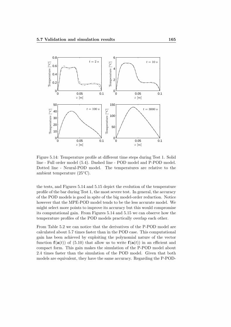
5.7 Validation and simulation results 165
0 0.05 0.10
0.2
0.4
0.6
0.8
0 0.05 0.10
2
4
6
0 0.05 0.10
10
20
30
40
50
0 0.05 0.10
50
100
150Tem
per
atu
re[◦
C]
Tem
per
atu
re[◦
C]
Tem
per
atu
re[◦
C]
Tem
per
atu
re[◦
C]
z [m]z [m]
z [m]z [m]
t = 2 s t = 10 s
t = 100 s t = 3000 s
Figure 5.14: Temperature profile at different time steps during Test 1. Solidline - Full order model (5.4). Dashed line - POD model and P-POD model.Dotted line - Neural-POD model. The temperatures are relative to theambient temperature (25◦C).
the tests, and Figures 5.14 and 5.15 depict the evolution of the temperatureprofile of the bar during Test 1, the most severe test. In general, the accuracyof the POD models is good in spite of the big model-order reduction. Noticehowever that the MPE-POD model tends to be the less accurate model. Wemight select more points to improve its accuracy but this would compromiseits computational gain. From Figures 5.14 and 5.15 we can observe how thetemperature profiles of the POD models practically overlap each other.
From Table 5.2 we can notice that the derivatives of the P-POD model arecalculated about 5.7 times faster than in the POD case. This computationalgain has been achieved by exploiting the polynomial nature of the vectorfunction f(a(t)) of (5.10) that allow us to write f(a(t)) in an efficient andcompact form. This gain makes the simulation of the P-POD model about2.4 times faster than the simulation of the POD model. Given that bothmodels are equivalent, they have the same accuracy. Regarding the P-POD-

166 Performance Improvement in Model Simulation
0 0.05 0.10
0.2
0.4
0.6
0.8
0 0.05 0.10
2
4
6
0 0.05 0.10
20
40
60
0 0.05 0.10
50
100
150
Tem
per
atu
re[◦
C]
Tem
per
atu
re[◦
C]
Tem
per
atu
re[◦
C]
Tem
per
atu
re[◦
C]
z [m]z [m]
z [m]z [m]
t = 2 s t = 10 s
t = 100 s t = 3000 s
Figure 5.15: Temperature profile at different time steps during Test 1. Solidline - Full order model (5.4). Dashed line - P-POD-RS model. Dottedline - MPE-POD model. The temperatures are relative to the ambienttemperature (25◦C).
RS model, the calculation of the derivatives is performed about 13.3 timesfaster than in the POD case and 2.3 times faster than in the P-POD case.This significant computational gain has been obtained by properly selectinga subset of monomials of the P-POD model. The impact of this gain on thesimulation time is also remarkable. The simulation of P-POD-RS requiresabout 3.6 times less time than the simulation of the POD model. In addition,the difference in their responses is very small. The largest difference occursduring Test 1, and this difference is only of 0.13◦C.
For the Neural-POD case, the derivatives are calculated around 9.7 timesfaster than in the POD model. This considerable gain has been achievedby approximating the vector function f(a(t)) with a multi-layer perceptron.The impact of this gain on the simulation time is such that the simulationof the Neural-POD model requires about 3.3 times less time than thesimulation of the POD model. Also notice that the difference between the
5.8 Conclusions 167
POD model and the Neural-POD model is very small. The largest differencein their responses arises in the course of Test 1, and this difference is merelyof 0.26◦C.
According to the results presented in Table 5.2, the P-POD-RS and Neural-POD models are in that order the fastest reduced-order models of the bar.Although the MPE-POD model was faster than the POD model, it wasneither as fast as the P-POD-RS, Neural-POD and P-POD models nor asaccurate as them. At this point it is important to emphasize that theMPE method is a general technique that does not exploit the particularcharacteristics of the kind of problems treated in this chapter, and thereforethe results obtained were expected. It is undoubted that the incorporation ofprior knowledge about a problem on a given algorithm improves the results.
5.8 Conclusions
In this chapter we have presented two methods for speeding up theevaluation of nonlinear POD models. In the first method, the nonlinearvector function of the POD models is approximated by a multi-layerperceptron which in general can be evaluated much faster than the originalvector function. In this approach both the computational gain and thecapability of learning accurately complex nonlinear mappings are limited bythe size of the network. The larger the MLP, the lesser is the computationalgain but the better is the ability of learning complex nonlinear mappings andvice versa. Therefore, the size of the net has to be chosen in such a way thatit provides a good trade-off between accuracy and computational gain. Oneof the main difficulties of this approach is to find a suitable number of hiddenneurons for the MLP. Additionally, since the neural networks suffer of thelocal minima problem, the training of the MLP has to be performed severaltimes starting from different initial conditions in order to make sure that thenetwork is not trapped in a local minimum. However, the convergence tothe global minimum can not be guaranteed. This problem gets worse as thenumber of neurons with nonlinear activation functions increases. Anotheraspect that we have to bear in mind, is that the approximation of the vectorfunction offered by the neural network is only valid within a specific range.Beyond this range the approximation fails, and the Neural-POD model isnot reliable anymore.
The second method is mostly aimed for accelerating nonlinear POD

168 Performance Improvement in Model Simulation
models derived from input-affine high-dimensional systems with polynomialnonlinearities. We have shown that by exploiting their polynomial nature,we can generate compact and efficient representations (P-POD models)which can be evaluated much faster than the POD models whose vectorfunctions require the full spatial information of the original model. Inaddition, we have discussed how the sequential feature selection algorithmscan help us to accelerate even more these P-POD models by selecting theirmost relevant monomials (suboptimal solution). Note that this approachmight be also employed in the case of input-affine high-dimensional systemswith non-polynomial nonlinearities, as long as these nonlinearities can beapproximated by low degree polynomials. This condition is advised in orderto keep the number of monomials as small as possible. A notable advantageof this approach with respect to the first method is that we have to solve aconvex optimization problem. However its drawback is that the number ofmonomials can be very large.
Furthermore in this chapter, we have discussed two ways of guaranteeing thelocal stability of POD models with polynomial nonlinearities. In our firstapproach we end up with an SDP optimization problem whose constraintprovides a sufficient condition for the local stability of the models. Theproblem of this method is that the constraint can be very conservative. Inthe second approach we finish up with an NSDP optimization problem whoseconstraints unlike the first approach, give necessary and sufficient conditionsfor the stability of the POD models. The drawback of this formulation is thatwe have to deal with a non-convex optimization problem. In both methodsthe local stability of the POD models is guaranteed independently of thedata used. However the quality of the reduced-order models still dependson the quality of data employed in the model reduction process.
Among the POD models derived for the bar, the simulation results showedthat the largest computational gains were obtained with the P-POD-RS andNeural-POD models. On one hand we have to point out that the success ofthe polynomial POD models resides in the fact of taking advantage of thepolynomial nature of the problem. On the other hand in the neural networkapproach, the nature of the problem is not exploited and consequently givenits general character, this method can be applied to a wider class of systems,although with the difficulties mentioned before.
Further research is necessary in order to evaluate the approaches proposedin this chapter on dynamic systems with harder nonlinearities.

Chapter 6
General Conclusions
6.1 Concluding remarks
This dissertation considers two main research subjects. First, it describes theapplication of a set of techniques such as proper orthogonal decomposition,Galerkin projection, model predictive control, Kalman filtering, and sum ofsquares decomposition (from theory of positive polynomials), to the design ofadvanced control schemes for tubular chemical reactors. Second, it discusseshow to improve the performance in model simulation of reduced-ordermodels derived by using proper orthogonal decomposition and Galerkinprojection from nonlinear high-dimensional systems, which are obtainedafter discretizing the nonlinear partial differential equations that modelmany processes.
Regarding the first research topic of this thesis, we have the followingconcluding remarks:
• The design of the predictive control schemes for the tubular reactortreated in this dissertation has been possible due to the significantmodel order reduction (from 600 states to only 20 states) achieved bymeans of the POD and Galerkin projection techniques.
• In spite of the linearization and discretization of the nonlinear PDEsthat model the reactor, and the dramatic model order reductionobtained using POD for generating the model on which the control
169

170 General Conclusions
systems proposed are based, the control schemes performed verywell when typical disturbances were applied to the reactor (Tests1 and 2 defined in Section 3.5). However, the performance of thecontrol schemes was compromised when the reactor was subjectedto large disturbances (Tests 3 and 4 described in Section 3.5). Thedegradation in their performance is mainly due to the fact that underlarge disturbances, the reactor operates far from the operating profileswhere the nonlinear model was linearized, and therefore the differencesbetween the nonlinear dynamics of the process and the linear PODmodel on which the control schemes are based become considerable.
• Typically, POD-based predictive controllers are formulated in termsof POD coefficients which have no physical meaning, and the controlof the variables of interest is achieved indirectly by controlling thesecoefficients. However, we have shown that formulations in terms ofphysical variables are suitable alternatives that make the tuning ofthe predictive controllers more intuitive and the definition of theircontrol goals more flexible.
• In Chapter 4, we have shown that the theory of positive polynomialsprovides a way of reducing the large number of state/output con-straints (linear inequalities) that usually characterizes the POD-basedpredictive controllers. In this approach the feasible region delimitedby the large set of inequality constraints is approximated by the onedelimited by a few linear matrix inequalities. It has been shown forthe case of the reactor that this methodology leads to a significantreduction in the number of temperature constraints which conducesto a considerable saving of memory. Nevertheless the computationaltime needed for solving the optimization of the predictive controllerbased on the LMI constraints, is much larger than the time required forsolving the original problem. The limitation comes from the fact thatthe LMI constraints introduce a large number of variables. It is clearthat with this positive polynomial approach the resulting optimizationproblem is more complex than the original one. However we wantto emphasize that this technique guarantees the fulfillment of thetemperature constraint at every point of the reactor.
• For reducing the large number of state/output constraints characteriz-ing the POD-based predictive controllers, we also proposed in Chapter4 a greedy algorithm which selects a reduced set of constraints fromthe full set, by exploiting the similarities between the coefficients of

6.1 Concluding remarks 171
consecutive constraints. This algorithm proved to be quite effectiveat the moment of being applied to one of the predictive controllersdesigned for the reactor. The number of temperature constraints wasreduced from 24 000 to only 1600, leading to a considerable savingof memory, and a substantial reduction in the computational timerequired for solving the optimization within the MPC controller. Inaddition, the behavior of the controller based on the reduced set ofconstraints was practically identical to the one based on the completeset. Note however that unlike the positive polynomial approach, we donot have any command on the temperature between the discretizationpoints.
Finally, we have the subsequent concluding remarks concerning the secondresearch subject of this dissertation:
• The use of a multilayer perceptron for approximating the nonlinearvector function of the POD models, has demonstrated to be a possibleway of speeding up their evaluation. However, the local minimaproblem in the training process of the network, can be a limiting factorof the applicability of this approach in systems with a considerableamount of POD coefficients.
• We have shown that the acceleration of POD models derived frominput-affine high-dimensional systems with polynomial nonlinearities,can be achieved by taking advantage of the polynomial nature of themodels for generating compact and efficient formulations (polynomialPOD models). In addition, the use of the sequential feature selectionalgorithms has proven to be quite useful for boosting the computa-tional gain of these polynomial POD models. Although this approachis mostly intended for systems with polynomial nonlinearities, it mightbe applied to models with non-polynomial nonlinearities providedthat these nonlinearities can be approximated well enough by lowdegree polynomials. In addition, it has been shown that by usingthe Lyapunov’s theory, the local stability of the resulting POD modelswith polynomial nonlinearities can be guaranteed.

172 General Conclusions
6.2 Future research
The research presented in this work can be further extended in severaldirections.
• Along Chapters 3 and 4, it has been pointed out that the tuning ofthe MPC controllers for the tubular reactor considered in this thesis,has been done in a conservative way (for being able to handle largedisturbances). In addition, it has been observed how the performanceof the control systems is degraded when large disturbances are appliedto the process. These issues are the consequence of not taking intoaccount the nonlinear nature of the reactor in the design of the controlschemes. Therefore, a natural extension of the predictive controlsystems proposed in this thesis, is the incorporation of the nonlinearcharacteristics of the process into the POD model on which they arebased.
• It is clear that the quality of a POD model depends on the quality ofthe data collected during the snapshot experiment, and this fact makesof the construction of the snapshot matrix a key step in the modelreduction process by POD. Many people [8, 40, 58, 87] have addressedseveral issues regarding the snapshots generation, but thus far, thereis not a definitive way to decide [13],
– How many snapshots are necessary for having good informationabout the system,
– How long the simulations should be run to generate the snapshots,
– Which initial conditions should be used, or
– How to incorporate control information (in the case of controlproblems).
Consequently the design of the snapshot experiment is still an openproblem that demands the attention of the researchers.
• Along this work we have not considered the dispersion/diffusionphenomena and the dynamics of the heat exchangers in the jacketsof the reactor. The inclusion of these characteristics into thereactor model would make it more realistic, and still not so specificthat it compromises the generality of the results and conceptualcontributions of the study. Therefore an extension of the presented

6.2 Future research 173
work would be the application and pertinent adjustment of thecontrol strategies and algorithms proposed thus far, to the case wherethe dispersion/diffusion phenomena and the dynamics of the heatexchangers are considered in the reactor model.
• In this dissertation we have addressed the problem of speeding up theevaluation of nonlinear POD models by using neural networks andby exploiting the polynomial nature of some systems. In spite of thegood results obtained, we can not say that we have found a definitivesolution to this problem, and consequently more research is needed inthis direction.
• For the case when POD is applied to multidimensional systems, thatis, systems with more than one spatial coordinate, the columns ofthe snapshot matrix are typically assembled by stacking the valuesof the physical variable at every grid point. This stacking procedureignores any possible Cartesian structure that may be present, andcommonly produces a snapshot matrix with a large number of rows.If the spatial domain has d coordinates and each of them has N gridpoints, the number of rows of the snapshot matrix is equal to Nd. Itis clear that the number of rows is typically an exponential functionof d, and this fact may make the computation of the basis vectorsproblematic when the number of grid points increases. In order totackle this situation, in [148, 153], an alternative spectral expansionto the one used in this thesis (and in most of the studies regardingPOD) is proposed, which takes into account the multidimensionalnature of the spatial coordinates by using a tensor representation.In this approach the basis vectors are computed using the Higher-Order Singular Value Decomposition (HOSVD) [88]. Alternatively in[149,150], a method known as tensor SVD is introduced for computingthe basis vectors. However, it should be clear that there is nota straightforward generalization of the algebraic concept of singularvalues and singular value decompositions to tensors or multi-wayarrays. Therefore more research regarding the derivation of optimalbasis vectors for multidimensional systems is required.


Bibliography
[1] O. M. Agudelo, M. Baes, J. J. Espinosa, M. Diehl, and B. De Moor. Positivepolynomial constraints for POD–based model predictive controllers. IEEETransactions on Automatic Control, 54(5):988–999, May 2009.
[2] O. M. Agudelo, J. J. Espinosa, and B. De Moor. Application of POD andpredictive control techniques to the control of the temperature profile of anone–dimensional bar. In Proceedings of the XII Latin–American Congress onAutomatic Control (CLCA 2006), pages 127–132, Salvador (Bahia), Brasil,October 2006.
[3] O. M. Agudelo, J. J. Espinosa, and B. De Moor. Control of a tubular chemicalreactor by means of POD and predictive control techniques. In Proceedingsof the European Control Conference 2007 (ECC’07), pages 1046–1053, Kos,Greece, July 2007.
[4] O. M. Agudelo, J. J. Espinosa, and B. De Moor. POD–based predictivecontroller with temperature constraints for a tubular reactor. In Proceedingsof the 46th IEEE Conference on Decision and Control (CDC 2007), pages3537–3542, New Orleans, USA, December 2007.
[5] O. M. Agudelo, J. J. Espinosa, and B. De Moor. Algorithm for reducing thenumber of constraints of POD–based predictive controllers. In Proceedingsof the 47th IEEE Conference on Decision and Control (CDC 2008), pages4743–4748, Cancun, Mexico, December 2008.
[6] O. M. Agudelo, J. J. Espinosa, and B. DeMoor. Acceleration of PODmodels with polynomial nonlinearities. Internal Report 09-81, ESAT-SISTA,K.U.Leuven (Leuven, Belgium), 2009. Submitted to IEEE Transactions onControl Systems Technology.
[7] O. M. Agudelo, J. J. Espinosa, and B. DeMoor. Acceleration of nonlinearPOD models: a neural network approach. In Proceedings of the EuropeanControl Conference 2009 (ECC’09), pages 1547–1552, Budapest, Hungary,August 2009.
[8] H. Aling, S. Banerjee, A. K. Bangia, V. Cole, J. Ebert, A. Emami-Naeini,K. F. Jensen, I. G. Kevrekidis, and S. Shvartsman. Nonlinear model reduction
175

176 Bibliography
for simulation and control of rapid thermal processing. In Proceedings of theAmerican Control Conference, volume 4, pages 2233–2238, Albuquerque, NewMexico, 1997.
[9] A. C. Antoulas. Approximation of Large-Scale Dynamical systems– Advancesin Design and Control. SIAM, Philadelphia, PA, USA, 2005.
[10] P. Astrid. Fast reduced order modeling technique for large scale LTV systems.In Proceedings of American Control Conference 2004, volume 1, pages 762–767, 2004.
[11] P. Astrid. Reduction of process simulation models: a proper orthogonaldecomposition approach. PhD thesis, Technishche Universiteit Eindhoven,Eindhoven (Netherlands), November 2004.
[12] P. Astrid, S. Weiland, K. Willcox, and T. Backs. Missing point estimation inmodels described by proper orthogonal decomposition. IEEE Transactionson Automatic Control, 53(10):2237–2251, November 2008.
[13] J. A. Atwell. Proper Orthogonal Decomposition for Reduced Order Controlof Partial Differential Equations. PhD thesis, Virginia Polytechnic Instituteand State University, Blacksburg, Virginia (USA), April 2000.
[14] J. A. Atwell and B. B. King. Proper orthogonal decomposition forreduced basis feedback controllers for parabolic equations. Mathematical andComputer Modelling, 33:1–19, 2001.
[15] J. A. Atwell and B. B. King. Reduced order controllers for spatiallydistributed systems via proper orthogonal decomposition. SIAM J. Sci.Comput., 26(1):128–151, 2005.
[16] Anil K. Bangia, Paul F. Batcho, Ioannis G. Kevrekidis, and George Em.Karniadakis. Unsteady two–dimensional flows in complex geometries:Comparative bifurcation studies with global eigenfunction expansions. SIAMJ. Sci. Comput., 18(3):775–805, 1997.
[17] H. T. Banks, R. C. H. del Rosario, and R. C. Smith. Reduced–order modelfeedback control design: Numerical implementation in a thin shell model.IEEE Transactions on Automatic Control, 45(7):1312–1324, July 2000.
[18] S. Basu, R. Pollack, and M.-F. Roy. On the combinatorial and algebraiccomplexity of quantifier elimination. J. ACM, 43(6):1002–1045, 1996.
[19] E. Beltrami. Sulle funzioni bilineari. Giornale di Matematiche ad Uso degliStudenti Delle Universita, 11:98–106, 1873.
[20] A. Ben-Tal and A. Nemirovski. Lectures on Modern Convex Optimization:Analysis, Algorithms, and Engineering Applications. MPS/SIAM Series onOptimization. SIAM, Philadelphia, USA, 2001.
[21] A. Ben-Tal and M. Zibulevsky. Penalty–barrier multiplier methods for convexprogramming problems. SIAM J. Optim., 7:347–366, 1997.

Bibliography 177
[22] G. Berkooz. Observations on the proper orthogonal decomposition. In T. B.Gatski, S. Sarkar, and C. G. Speziale, editors, Studies in Turbulence, pages229–247, New York, 1991. Springer–Verlag.
[23] G. Berkooz, P. J. Holmes, and J. L. Lumley. The proper orthogonaldecomposition in the analysis of turbulent flows. Annu. Rev. Fluid Mech.,25:539–575, 1993.
[24] P. Beyer, S. Benkadda, and X. Garbet. Proper orthogonal decompositionand Galerkin projection for a three–dimensional plasma dynamical system.Physical Review E, 61(1):813–823, Jan 2000.
[25] A.M Blanco and J.A. Bandoni. Optimal design of stable process. Lat. Am.Appl. Res., 33(2):123–128, 2003.
[26] L. G. Bleris and M. V. Kothare. Reduced order distributed boundary controlof thermal transients in microsystems. IEEE Transactions on control systemstechnology, 13(6):853–867, November 2005.
[27] J. Bochnak, M. Coste, and M.-F. Roy. Real Algebraic Geometry. Sringer,1998.
[28] N. K. Bose. Applied multidimensional systems theory. Van NostrandReinhold, 1982.
[29] S. Boyd and L. Vandenberghe. Convex Optimization. Cambridge UniversityPress, United Kingdom, 2004.
[30] A. Brandolin, M. Lacunza, P. Ugrin, and N. Capiati. High pressurepolymerization of ethylene. an improved mathematical model for industrialtubular reactors. Polymer Reaction Engineering, 4:193–241, 1996.
[31] D. H. Chambers, R. J. Adrian, P. Moin, D. S. Stewart, and H. J. Sung.Karhunen–loeve expansion of burgers’ model of turbulence. Phys. Fluids,31(9):2573–2582, September 1988.
[32] A. Chatterjee. An introduction to the proper orthogonal decomposition.Current Science, 78(7):808–817, April 2000.
[33] P. D. Christofides. Robust control of parabolic PDE systems. ChemicalEngineering Science, 53(16):2949 – 2965, 1998.
[34] P. D. Christofides. Nonlinear and Robust Control of PDE Systems. Methodsand Applications to Transport–Reaction Processes. Systems & Control:Foundations & Applications. Birkhauser, 2001.
[35] P. D. Christofides and P. Daoutidis. Feedback control of hyperbolic PDEsystems. AIChE Journal, 42:3063 – 3086, 1996.
[36] P. D. Christofides and P. Daoutidis. Robust control of hyperbolic PDEsystems. Chemical Engineering Science, 53(1):85 – 105, 1998.

178 Bibliography
[37] J. P. Cusumano, M. T. Sharkady, and B. W. Kimble. Experimentalmeasurements of dimensionality and spatial coherence in the dynamics ofa flexible-beam impact oscillator. Philosophical Transactions: PhysicalSciences and Engineering, 347(1683):421–438, May 1994.
[38] C. R. Cutler and B. L. Ramaker. Dynamic matrix control - a computercontrol algorithm. In AIChE National Meeting, Houston, TX, 1979.
[39] P. Danckwertz. Continuous flow systems. Chemical Engineering Science,2:1–13, 1953.
[40] A. E. Deane, I. G. Kevrekidis, G. E. Karniadakis, and S. A. Orszag. Low-dimensional models for complex geometry flows: application to groovedchannels and circular cylinders. Phys. Fluids A, 3(10):2337–2354, October1991.
[41] D. Del Vecchio and N. Petit. Boundary control for an industrial under–actuated tubular chemical reactor. Journal of Process Control, 15:771–784,2005.
[42] M. Diehl, F. Jarre, and C. Vogelbusch. Loss of superlinear convergence for anSQP–type method with conic constraints. SIAM Journal on Optimization,16(4):1201–1210, 2006.
[43] J. R. Dormand and P. J. Prince. A family of embedded runge-kutta formulae.J. Comp. Appl. Math., 6:19–26, 1980.
[44] S. Dubljevic and P. D. Christofides. Predictive output feedback control ofparabolic partial differential equations (PDEs). Industrial & EngineeringChemistry Research, 45(25):8421–8429, 2006.
[45] S. Dubljevic and P. D. Christofides. Predictive output feedback control ofparabolic PDEs. In Proceedings of the American Control Conference 2006,pages 1155–1160, Minneapolis, Minnesota, USA, June 2006.
[46] S. Dubljevic, P. Mhaskar, N. H. El-Farra, and P. D. Christofides.Predictive control of transport-reaction processes. Computers and ChemicalEngineering, 29(11–12):2335–2345, 2005.
[47] M. Fahl. Computation of POD basis functions for fluid flows with lanczosmethods. Math. Comput. Modeling, 34:91–1078, 2001.
[48] M. Fahl and E. W. Sachs. Reduced order modelling approaches to PDE–constrained optimization based on proper orthogonal decomposition. In L. T.Biegler, O. Ghattas, M. Heinkenschloss, and B. van Bloemen Waanders,editors, Large–Scale PDE–Constrained Optimization, pages 268–280, Heidel-berg, Germany, 2003. Springer–Verlag.
[49] F. Fang, C. C. Pain, I. M. Navon, G. J. Gorman, M. D. Piggott, P. A. Allison,P.E. Farrell, and A. J. H. Goddard. A POD reduced order unstructuredmesh ocean modelling method for moderate reynolds number flows. OceanModelling, 28(1–3):127–136, 2009.

Bibliography 179
[50] B. Fares, D. Noll, and P. Apkarian. Robust control via sequential semidefiniteprogramming. SIAM Journal on Control and Optimization, 40(6):1791–1820,2002.
[51] B. F. Feeny and R. Kappagantu. On the physical interpretation of properorthogonal modes in vibrations. Journal of Sound and Vibration, 211(4):607–616, 1998.
[52] R. Quinta Ferreira, C. Costa, and S. Masetti. Reverse-flow reactor for aselective oxidation process. Chemical Engineering Science, 54:4615–4627,1999.
[53] M. Fjeld and B. Ursin. Approximate lumped models of a tubular chemicalreactor, and their use in feedback and feedforward control. In Proceedings ofthe 2nd IFAC Symposium on Multivariable Technical Control Systems, pages1–18, North Holland, Amsterdam, 1971.
[54] G.F. Franklin, J.D. Powell, and M.L. Workman. Digital Control of DynamicSystems. Addison-Wesley, second edition, 1990.
[55] R. W. Freund and F. Jarre. A sensitivity analysis and a convergence resultfor a sequential semidefinite programming method. Technical report, BellLaboratories, Murray Hill, New Jersey, USA, 2003.
[56] C. E. Garcıa, D. M. Prett, and M. Morari. Model predictive control: Theoryand practice-a survey. Automatica, 25(3):335–348, 1989.
[57] P. E. Gill, W. Murray, and M. H. Wright. Practical Optimization. AcademicPress, London, UK, 1981.
[58] M. D. Graham and I. G. Kevrekidis. Alternative approaches to the karhunen–loeve decomposition for model reduction and data analysis. Computers Chem.Eng., 20(5):495–506, 1996.
[59] W. R. Graham, J. Peraire, and K. Y. Tang. Optimal control of vortexshedding using low–order models. Part I–open–loop model development.International Journal for Numerical Methods in Engineering, 44(7):945–972,1999.
[60] M. M. Gupta, L. Jin, and N. Homma. Static and Dynamic Neural Networks:From Fundamentals to Advanced Theory. Wiley–IEEE press, April 2003.
[61] I. Guyon and A. Elisseeff. An introduction to variable and feature selection.Journal of Machine Learning Research, 3:1157–1182, 2003.
[62] M. T. Hagan and M. Menhaj. Training feed–forward networks with theMarquardt algorithm. IEEE Transactions on Neural Networks, 5(6):989–993,1994.
[63] S. Haykin. Neural Networks, a comprehensive foundation. Prentice Hall,Upper Saddle River, New jersey, 1999.

180 Bibliography
[64] M. Hazenberg, P. Astrid, and S. Weiland. Low order modeling and optimalcontrol design of a heated plate. In Proceedings of the 5th European ControlConference, Cambridge, September 2003.
[65] D. Henrion, J. Lofberg, Michal Kocvara, and Michael Stingl. Solvingpolynomial static output feedback problems with PENBMI. In Proceedingsof the 44th IEEE Conference on Decision and Control, and the EuropeanControl Conference 2005, pages 7581–7586, Seville, Spain, December 2005.
[66] P. Holmes, J. L. Lumley, and G. Berkooz. Turbulence, Coherence Structure,Dynamical Systems and Symmetry. Cambridge University Press, Cambridge,1996.
[67] K. Hornik, M. Stinchcombe, and H. White. Multilayer feedforward networksare universal approximators. Neural Networks, 2:359–366, 1989.
[68] M. Hovd and R. D. Braatz. Handling state and output constraints inMPC using time–dependent weights. In Proceedings of the American ControlConference (ACC), Arlington, USA, 2001.
[69] M. Hovd and R. D. Braatz. On the use of soft constraints in MPC controllersfor plants with inverse response. In Proceedings of the 6th IFAC symposiumon Dynamics and control of process Systems, Jejudo Island, Korea, 2001.
[70] L. Huisman. Control of glass melting processes based on reduced CFD models.PhD thesis, Technishche Universiteit Eindhoven, Eindhoven (Netherlands),March 2005.
[71] L. Huisman and S. Weiland. Identification and model predictive control of anindustrial glass feeder. In Proceedings of the 13th IFAC Symposium on SystemIdentification (SYSID–2003), pages 1685–1689, Rotterdam, The Netherlands,August 2003.
[72] L. Huisman and S. Weiland. Reduced model based LQG control of anindustrial glass feeder. In Proceedings of the 10th IFAC/IFORS/IMACS/IFIPSymposium on Large Scale Systems: Theory and Applications, volume 1,pages 421–426, Osaka, Japan, July 2004.
[73] A. Iollo, S. Lanteri, and J. A. Desideri. Stability properties of POD–Galerkinapproximations for the compressible Navier–Stokes equations. Theoreticaland Computational Fluid Dynamics, 13(6):377–396, March 2000.
[74] I. T. Jollife. Principal Component Analysis. Springer-Verlag, New York, 1986.
[75] C. Jordan. Memoire sur les formes bilineaires. J. Math. Pures Appl.,Deuxieme Serie, 19:35–54, 1874.
[76] C. Jordan. Sur la reduction des formes bilineaires. Comptes Rendus del’Academie Sciences, Paris, 78:614–617, 1874.
Bibliography 181
[77] R. E. Kalman. A new approach to linear filtering and prediction problems.Transactions ASME, Series D, Journal of basic engineering, 82:34–45, March1960.
[78] G. M. Kepler, H. T. Tran, and H. T. Banks. Reduced order modelcompensator control of species transport in a CVD reactor. Optimal ControlApplication & Methods, 21(4):143–160, 2000.
[79] M. Kirby, J. P. Boris, and L. Sirovich. A proper orthogonal decompositionof a simulated supersonic shear layer. Int. J. Numerical Methods Fluids,10:411–428, 1990.
[80] M. Kirby and L. Sirovich. Application of the karhunen-loeve procedure forthe characterization of human faces. IEEE Transactions on Pattern Analysisand Machine Intelligence, 12(1):103–108, 1990.
[81] R. Kohavi and H. John. Wrappers for feature subset selection. ArtificialIntelligence, 97(1–2):273–324, 1997.
[82] D. D. Kosambi. Statistics in function space. J. Indian Math. Soc., 7:76–88,1943.
[83] M. Kocvara and M. Stingl. PENNON – a code for convex nonlinear andsemidefinite programming. Opt. Methods and Software, 20(3):317–333, 2003.
[84] E. Kreuzer and O. Kust. Proper orthogonal decompositionan efficient meansof controlling self-excited vibrations of long torsional strings. In Proceedingsof the 1996 ASME International Mechanical Engineering Congress andExposition, pages 105–110, 1996.
[85] K. Kunisch and S. Volkwein. Control of the burgers equation by areduced–order approach using proper orthogonal decomposition. Journal ofOptimization Theory and Applications, 102(2):345–371, August 1999.
[86] H. Kwakernaak and R. Sivan. Linear optimal control systems. Wiley-Interscience, 1972.
[87] S. Lall, J. E. Marsden, and S. Glavaski. Empirical model reduction ofcontrolled nonlinear systems. Technical Report CIT-CDS-98-008, Controland Dynamical Systems, California Institute of Technology, June 1998.
[88] L. De Lathauwer, B. De Moor, and J. Vandewalle. A multilinear singularvalue decomposition. SIAM Journal of Matrix Analysis and Applications,21(4):1253–1278, 2000.
[89] J. H. Lee and B. Cooley. Recent advances in model predictive control andother related areas. In J. C. Kantor, C. E. Garcia, and B. Carnahan, editors,Proceedings of the Fifth international conference on chemical process controlAICHE and CACHE, pages 201–216, 1997.

182 Bibliography
[90] A. Liakopoulos, P. A. Blythe, and H. Gunes. A reduced dynamical modelof convective flows in tall laterally heated cavities. Proceedings of the RoyalSociety A: Mathematical, Physical and Engineering Sciences, 453(1958):663–672, 1997.
[91] Y. C. Liang, H. P. Lee, S. P. Lim, W. Z. Lin, K. H. Lee, and C. G. Wu. Properorthogonal decomposition and its applications–Part I: Theory. Journal ofSound and Vibration, 252(3):527–544, May 2002.
[92] Y. C. Liang, H. P. Lee, S. P. Lim, W. Z. Lin, K. H. Lee, and C. G. Wu. Properorthogonal decomposition and its applications–Part II: Model reduction forMEMS dynamical systems. Journal of Sound and Vibration, 256(3):515–532,2002.
[93] W. Z. Lin, Y. J. Zhang, and E. P. Li. Proper orthogonal decomposition inthe generation of reduced order models for interconnects. IEEE Transactionson Advanced Packing, 31(3):627–636, 2008.
[94] M. Loeve. Probability Theory. D. Van Nostrand Company, Inc, New Jersey,second edition, 1960.
[95] F. Logist. Model based optimization and control of chemical reactors withdistributed parameters. PhD thesis, Katholieke Universiteit Leuven, Leuven(Belgium), January 2008.
[96] D. G. Luenberger. An introduction to observers. IEEE transactions onAutomatic Control, 16(6):596–602, December 1971.
[97] J. Lumley and P. Blossey. Control of turbulence. Annual Review of FluidMechanics, 30:311–327, 1998.
[98] J. L. Lumley. Stochastic Tools in Turbulence. Academic Press, New York,1970.
[99] H. V. Ly and H. T. Tran. Modeling and control of physical processes usingproper orthogonal decomposition. Journal of Mathematical and ComputerModeling, 33:223–236, 2001.
[100] H. V. Ly and H. T. Tran. Proper orthogonal decomposition for flowcalculations and optimal control in a horizontal CVD reactor. Quarterlyof Applied Mathematics, 60:631–656, 2002.
[101] Mathworks, USA. Optimization Toolbox 3: user’s guide, 2006.
[102] Mathworks, USA. Neural Network Toolbox 6. User’s guide, 2008.
[103] D. Q. Mayne. Nonlinear model predictive control: An assessment. In J. C.Kantor, C. E. Garcia, and B. Carnahan, editors, Proceedings of the Fifthinternational conference on chemical process control AICHE and CACHE,pages 217–231, 1997.

Bibliography 183
[104] D. Q. Mayne, J. B. Rawlings C. V. Rao, and P. O. M. Scokaert. Constrainedmodel predictive control: Stability and optimality. Automatica, 36:789–814,2000.
[105] A. Miller. Subset Selection in Regression. Monographs on Statistics andApplied Probability 95. Chapman & Hall/CRC, Boca Raton, FL, secondedition, 2002.
[106] B. Mishra. Algorithmic Algebra. Sringer-verlag, 1999.
[107] M. Morari and J. H. Lee. Model predictive control: The good, the bad, andthe ugly. In Y. Arkun and W. H. Ray, editors, Chemical Process Control (CPCIV). Forth International Conference on Chemical Process Control, pages 419–444, Amsterdan, 1991. Elsevier.
[108] K. G. Murty and S. N. Kabadi. Some NP–complete problems in quadraticand nonlinear programming. Mathematical Programming, 39:117–129, 1987.
[109] K. R. Muske and J. B. Rawlings. Model predictive control with linear models.AIChE Journal, 39(2):262–287, 1993.
[110] T. Nakamura, S. Takamura, and M. Asada. Behaviour–based maprepresentation for a sonar–based mobile robot by statistical methods. InProceedings of the 1996 IEEE/RSJ International Conference on IntelligentRobots and Systems ’96 (IROS 96), volume 1, pages 276–283, Osaka, Japan,Nov. 1996.
[111] Y. Nesterov. Squared functional systems and optimization problems. InH. Frenk, K. Roos, T. Terlaky, and S. Zhang, editors, High PerformanceOptimization, pages 405–440. Kluwer Academic Publishers, 2000.
[112] Y. Nesterov and M. Todd. Self–scaled barriers and interior–point methods forconvex programming. Mathematics of Operations Research, 22:1–42, 1997.
[113] P. Van Overschee and B. De Moor. Subspace Identification of Linear Systems:Theory, Implementation, Applications. Kluwer Academic Publishers, 1996.
[114] G. Pannocchia and J. B. Rawlings. Robustness of MPC and disturbancemodels for multivariable ill–conditioned processes. Technical Report 2001–02,University of Wisconsin–Madison, Madison, WI 53706 (U.S.A), May 2001.
[115] A. Papachristodoulou and S. Prajna. A tutorial on sum of squares techniquesfor systems analysis. In Proceedings of the American Control Conference 2005,volume 4, pages 2686–2700, Portland, Oregon, USA, June 2005.
[116] T. W. Parks and C. S. Burrus. Digital Filter Design. John Wiley & Sons,New York, USA, 1987.
[117] P. A. Parrilo. Structured Semidefinite Programs and Semialgebraic GeometryMethods in Robustness and Optimization. PhD thesis, California Institute ofTechnology, USA, 2000.
184 Bibliography
[118] K. Pearson. On lines and planes of closest fit to systems of points in space.Philosophical Magazine, 2(6):559–572, 1901.
[119] S. Prajna. POD model reduction with stability guarantee. In Proceedings of42nd IEEE Conference on Decision and Control (CDC 2003), Hawaii, USA,December 2003.
[120] S. J. Qina and T. A. Badgwell. A survey of industrial model predictive controltechnology. Control Engineering Practice, 11:733–764, 2003.
[121] S. S. Ravindran. A reduced–order approach for optimal control of fluidsusing proper orthogonal decomposition. International Journal for NumericalMethods in Fluids, 34(5):425–448, November 2000.
[122] J. B. Rawlings and J. G. Ekerdt. Chemical Reactor Analysis and DesignFundamentals. Nob Hill Publishing, Madison, Wisconsin, 2002.
[123] J. B. Rawlings, E. S. Meadows, and K. Muske. Nonlinear model predictivecontrol: a tutorial and survey. In Proceedings of the IFAC Symposium onAdvanced Control of Chemical Processes, pages 203–214, Kyoto, Japan, 1994.
[124] Bruce Reznick. Some concrete aspects of Hilbert’s 17th problem. In InContemporary Mathematics, pages 251–272. American Mathematical Society,2000.
[125] J. Richalet, A. Rault, J. Testud, and J. Papon. Model predictive heuristiccontrol: Applications to industrial processes. Automatica, 14:413–428, 1978.
[126] N. L. Ricker. Model predictive control: State of the art. In Y. Arkun andW. H. Ray, editors, Chemical Process Control (CPC IV). Forth InternationalConference on Chemical Process Control, pages 271–296, Amsterdan, 1991.Elsevier.
[127] U. T. Ringertz. Eigenvalues in optimal structural design. In A.R Conn,L. T. Biegler, T. F. Coleman, and F. Santosa, editors, Proceedings of an IMAWorkshop on Large–Scale Optimizatioin, pages 135–149, 1997.
[128] J. A. Rossiter. Model-Based Predictive Control. A practical Approach. CRCPress, Boca Raton, Florida, USA, 2003.
[129] R. Ruotolo and C. Surace. Using SVD to detect damage detection instructures with different operational conditions. Journal of Sound andVibration, 226(3):425–439, 1999.
[130] E. Schmidt. Zur theorie der linearen und nichtlinearen integralgleichungen.I. Teil. Entwicklung willkurlicher funktionen nach system vorgeschriebener.Math. Ann., 63:433–476, 1907.
[131] P. O. M. Scokaert and J. B. Rawlings. Feasibility issues in linear modelpredictive control. AIChE Journal, 45:1649–1659, 1999.
[132] L. F. Shampine and M. E. Hosea. Analysis and implementation of TR–BDF2.Applied Numerical Mathematics, 20:21–37, 1996.

Bibliography 185
[133] H. Shang, J. Forbes, and M. Guay. Model predictive control for quasilinearhyperbolic distributed parameter systems. Industrial and EngineeringChemistry Research, 43(16):2140–2149, 2004.
[134] L. Sirovich. Turbulence and the dynamics of coherent structures. PartI: coherent structures. Part II: symmetries and transformations. Part III:dynamics and scaling. Quart. Appl. Math., 45:561–590, 1987.
[135] L. Sirovich and M. Kirby. Low–dimensional procedure for the characterizationof human faces. J. Opt. Soc. Am. A, 4(3):519–524, 1987.
[136] L. Sirovich, B. W. Knight, and J. D. Rodriguez. Optimal low-dimensionaldynamical approximations. Quarterly of Applied Mathematics, 48(3):535–548,September 1990.
[137] I. Y. Smets, D. Dochain, and J. F. Van Impe. Optimal temperature control ofa steady–state exothermic plug–flow reactor. AIChE Journal, 48 (2):279–286,2002.
[138] I. Y. Smets and J. F. Van Impe. Optimal control of tubular chemicalreactors: performance assessment under transient and diffuse conditions.In Proceedings of the 10th Mediterranean Conference on Control andAutomation – MED2002, Lisbon, Portugal, 2002.
[139] G. W. Stewart. On the early history of the singular value decomposition.SIAM review, 35(4):551–566, December 1993.
[140] J. Sturm. Using SeDuMi 1.02, a MATLAB toolbox for optimization oversymmetric cones. Optimization Methods and Software, 11:625–653, 1999.
[141] J. J. Sylvester. A new proof that a general quadric may be reduced to itscanonical form (that is, a linear function of squares) by means of a realorthogonal substitution. Messenger of Mathematics, 19:1–5, 1889.
[142] J. J. Sylvester. On the reduction of a bilinear quantic of the nth order to theform of a sum of n products by a double orthogonal substitution. Messengerof Mathematics, 19:42–46, 1889.
[143] J. J. Sylvester. Sur la reduction biorthogonale d’une forme lineo-lineaire a saforme cannonique. Comptes Rendus de l’Academie Sciences, Paris, 108:651–653, 1889.
[144] J. C. Tannehill, D. A. Anderson, and R. H. Pletcher. ComputationalFluid Mechanics and Heat Transfer. Series in Computational and PhysycalProcesses in Mechanics and Thermal Sciences. Taylor & Francis, USA, secondedition, 1997.
[145] P. Tatjewski and M. �Lawrynczuk. Soft computing in model–based predictivecontrol. Int. J. Appl. Math. Comput. Sci., 16(1):7–26, 2006.

186 Bibliography
[146] A. Theodoropoulou, R. A Adomaitis, and E. Zafiriou. Model reduction foroptimization of rapid thermal chemical vapor deposition systems. IEEETransactions on Semiconductor Manufacturing, 11(1):85–98, February 1998.
[147] E.F Toro. Riemann Solvers and Numerical Methods for Fluid Dynamics. Apractical Introduction. Springer–Verlag, Heidelberg, Germany, second edition,1999.
[148] F. van Belzen. Model reduction through proper orthogonal decompositions formultidimensional systems. In Book of abstracts of the 26th Benelux meetingon Systems and Control, page 152, Lommel, Belgium, March 2007.
[149] F. van Belzen. Analysis and approximation of multi-way arrays throughsingular value decompositions. In Book of abstracts of the 27th Beneluxmeeting on Systems and Control, page 103, Heeze, The Netherlands, March2008.
[150] F. van Belzen, S. Weiland, and J. de Graaf. Singular value decompositionsand low rank approximations of multi-linear functionals. In Proceedings ofthe 46th IEEE conference on Decision and Control, pages 3751–3756, NewOrleans, USA, December 2007.
[151] S. Volkwein and A. Hepberger. Impedance identification by POD model re-duction techniques (impedanz-identifikation mittels POD modellreduktion).at - Automatisierungstechnik, 56(8):437–446, August 2008.
[152] A. Webb. Statistical Pattern Recognition. John Wiley & Sons, LTD, secondedition, July 2002.
[153] S. Weiland and F. van Belzen. Model reduction through multilinearsingular value decompositions. In Proceedings of the European Conferenceon Computational Dynamics ECCOMAS CFD 2006, Egmond aan Zee, TheNetherlands, September 2006.
[154] H. Weyl. Das asymptotische verteilungsgesetz der eigenwert linearerpartieller differentialgleichungen (mit einer anwendung auf der theorie derhohlraumstrahlung). Math. Ann., 71:441–479, 1912.
[155] W. Y. Yang, W. C., T. S. Chung, and J. Morris. Applied Numerical Methodsusing Matlab. Wiley–Interscience, 2005.
[156] A. Yousefi, B. Lohmann, J. Lienemann, and J. G. Korvink. Nonlinearheat tranfer modelling and reduction. In Proceedings of the 12th IEEEMediterranean Conference on Control and Automation (MED ’04), Kusadasi,Turkey, June 2004.

Curriculum Vitae
Oscar Mauricio Agudelo Manozca was born in Cali, Colombia, in January1974. In 1997, he received the degree of Electronics Engineer from theUniverisidad Autonoma de Occidente, Cali, Colombia, and in 2004, hereceived the master degree in Industrial Control Engineering from theUniversidad de Ibague in cooperation with the Katholieke UniversiteitLeuven and the Universiteit Gent, Ibague, Colombia. His master thesis wasentitled “Control of a helicopter laboratory process using linear and fuzzytechniques”. From 1997 to 2004, he worked at the Universidad Autonomade Occidente as a full time teacher of control and automation. In October2004, he moved to Leuven in order to start his predoctoctal stage in theKatholieke Universiteit Leuven. During this period he worked alongsidethree companies, IPCOS (from Belgium), Protomation (from Netherlands)and Stamicarbon (from Netherlands) in a research project entitled “Controlof the synthesis section of a urea plant using MPC control techniques”. In2005, he started the Ph.D program in the SCD/SISTA research divisionof the Electrical Engineering Department of the K.U.Leuven, under thesupervision of Prof. Dr. Ir. Bart De Moor, Prof. Dr. Ir. Jairo Espinosaand Prof. Dr. Ir. Joos Vandewalle.
187


Publications by the author
Journal Papers
• O. M. Agudelo, M. Baes, J. J. Espinosa, M. Diehl and B. De Moor. Positivepolynomial constraints for POD-based model predictive controllers. IEEETransactions on Automatic Control, 54(5):988–999, May 2009.
• O. M. Agudelo, J. J. Espinosa and J. Vandewalle. Control of a helicopterlaboratory process using fuzzy techniques. Internal Report 06-74, ESAT-SISTA, K.U.Leuven (Leuven, Belgium), 2006. Accepted for publication inJournal of Intelligent & Fuzzy Systems: Applications in Engineering andTechnology.
• O. M. Agudelo, J. J. Espinosa and B. De Moor. Acceleration of PODmodels with polynomial nonlinearities. Internal Report 09-81, ESAT-SISTA,K.U.Leuven (Leuven, Belgium), 2009. Submitted to IEEE Transactions onControl Systems Technology.
International Conference Papers
• O. M. Agudelo, J. J. Espinosa and J. Vandewalle. Control of the synthesissection of a urea plant by means of an MPC controller. In W. Marquardt,and C. Pantelides, editors, Proceedings of the 16th European Symposiumon Computer Aided Process Engineering and 9th International Symposiumon Process Systems Engineering, volume 21 of Computer-Aided ChemicalEngineering, pages 1305–1310. Elsevier, 2006.
• O. M. Agudelo, J. J. Espinosa and B. De Moor. Application of POD andpredictive control techniques to the control of the temperature profile of anone-dimensional bar. In Proceedings of the XII Latin-American Congress onAutomatic Control (CLCA 2006), pages 127–132, Salvador, Brazil, October2006.
189
190 Bibliography
• O. M. Agudelo, J. J. Espinosa and B. De Moor. Control of a tubular chemicalreactor by means of POD and predictive control techniques. In Proceedingsof the European Control Conference 2007 (ECC’07), pages 1046–1053, Kos,Greece, July 2007.
• O. M. Agudelo, J. J. Espinosa and B. De Moor. POD-based predictivecontroller with temperature constraints for a tubular reactor. In Proceedingsof the 46th IEEE Conference on Decision and Control (CDC 2007), pages3537–3542, New Orleans, USA, December 2007.
• O. M. Agudelo, J. J. Espinosa and B. De Moor. Algorithm for reducing thenumber of constraints of POD-based predictive controllers. In Proceedingsof the 47th IEEE Conference on Decision and Control (CDC 2008), pages4743–4748, Cancun, Mexico, December 2008.
• O. M. Agudelo, J. J. Espinosa and B. De Moor. Acceleration of nonlinearPOD models: a neural network approach. In Proceedings of the EuropeanControl Conference 2009 (ECC’09), pages 1547–1552, Budapest, Hungary,August 2009.
Published Abstracts
• O. M. Agudelo, J. J. Espinosa and B. De Moor. Control of a tubular reactorusing POD and MPC. In Book of Abstracts of the 26th Benelux Meeting onSystems and Control, page 171, Lommel, Belgium, March 2007.
Internal Reports
• O. M. Agudelo, J. J. Espinosa and J. Vandewalle. Control of the synthesissection of a urea Plant using MPC control techniques. Internal Report 05-157, ESAT-SISTA, K.U.Leuven (Leuven, Belgium), 2005.
• O. M. Agudelo, J. J. Espinosa and J. Vandewalle. Application of predictivecontrol techniques to the synthesis section of a urea plant. Internal Report05-213, ESAT-SISTA, K.U.Leuven (Leuven, Belgium), 2005.
Related Documents