14-1 14 14 Dynamic Networks Objectives 14-1 Theory and Examples 14-2 Layered Digital Dynamic Networks 14-3 Example Dynamic Networks 14-5 Principles of Dynamic Learning 14-8 Dynamic Backpropagation 14-12 Preliminary Definitions 14-12 Real Time Recurrent Learning 14-12 Backpropagation-Through-Time 14-22 Summary and Comments on Dynamic Training 14-30 Summary of Results 14-34 Solved Problems 14-36 Epilogue 14-45 Further Reading 14-46 Exercises 14-47 Objectives Neural networks can be classified into static and dynamic categories. The multilayer network that we have discussed in the last three chapters is a static network. This means that the output can be calculated directly from the input through feedforward connections. In dynamic networks, the output depends not only on the current input to the network, but also on the current or previous inputs, outputs or states of the network. For example, the adaptive filter networks we discussed in Chapter 10 are dynamic net- works, since the output is computed from a tapped delay line of previous inputs. The Hopfield network we discussed in Chapter 3 is also a dynamic network. It has recurrent (feedback) connections, which means that the current output is a function of outputs at previous times. We will begin this chapter with a brief introduction to the operation of dynamic net- works, and then we will describe how these types of networks can be trained. The train- ing will be based on optimization algorithms that use gradients (as in steepest descent and conjugate gradient algorithms) or Jacobians (as in Gauss-Newton and Levenberg- Marquardt algorithms) These algorithms were described in Chapters 10, 11 and 12 for static networks. The difference between the training of static and dynamic networks is in the manner in which the gradient or Jacobian is computed. In this chapter, we will present methods for computing gradients for dynamic networks.

Welcome message from author
This document is posted to help you gain knowledge. Please leave a comment to let me know what you think about it! Share it to your friends and learn new things together.
Transcript
Objectives
14-1
14
14 Dynamic NetworksObjectives 14-1Theory and Examples 14-2
Layered Digital Dynamic Networks 14-3Example Dynamic Networks 14-5
Principles of Dynamic Learning 14-8Dynamic Backpropagation 14-12
Preliminary Definitions 14-12Real Time Recurrent Learning 14-12Backpropagation-Through-Time 14-22
Summary and Comments on Dynamic Training 14-30Summary of Results 14-34Solved Problems 14-36Epilogue 14-45Further Reading 14-46Exercises 14-47
ObjectivesNeural networks can be classified into static and dynamic categories. The multilayer network that we have discussed in the last three chapters is a static network. This means that the output can be calculated directly from the input through feedforward connections. In dynamic networks, the output depends not only on the current input to the network, but also on the current or previous inputs, outputs or states of the network. For example, the adaptive filter networks we discussed in Chapter 10 are dynamic net-works, since the output is computed from a tapped delay line of previous inputs. The Hopfield network we discussed in Chapter 3 is also a dynamic network. It has recurrent (feedback) connections, which means that the current output is a function of outputs at previous times.
We will begin this chapter with a brief introduction to the operation of dynamic net-works, and then we will describe how these types of networks can be trained. The train-ing will be based on optimization algorithms that use gradients (as in steepest descent and conjugate gradient algorithms) or Jacobians (as in Gauss-Newton and Levenberg-Marquardt algorithms) These algorithms were described in Chapters 10, 11 and 12 for static networks. The difference between the training of static and dynamic networks is in the manner in which the gradient or Jacobian is computed. In this chapter, we will present methods for computing gradients for dynamic networks.
14 Dynamic Networks
14-2
D
Theory and ExamplesDynamic networks are networks that contain delays (or integrators, for continuous-time networks) and that operate on a sequence of inputs. (In other words, the ordering of the inputs is important to the operation of the network.) These dynamic networks can have purely feedforward connections, like the adaptive filters of Chapter 10, or they can also have some feedback (recurrent) connections, like the Hopfield network of Chapter 3. Dynamic networks have memory. Their response at any given time will depend not only on the current input, but on the history of the input sequence.
Because dynamic networks have memory, they can be trained to learn sequential or time-varying patterns. This has applications in such diverse areas as control of dynam-ic systems, prediction in financial markets, channel equalization in communication systems, phase detection in power systems, sorting, fault detection, speech recogni-tion, learning of grammars in natural languages, and even the prediction of protein structure in genetics.
Dynamic networks can be trained using the standard optimization methods that we have discussed in Chapters 9 through 12. However, the gradients and Jacobians that are required for these methods cannot be computed using the standard backpropaga-tion algorithm. In this chapter we will present the dynamic backpropagation algorithms that are required for computing the gradients for dynamic networks.
There are two general approaches (with many variations) to gradient and Jacobian cal-culations in dynamic networks: backpropagation-through-time (BPTT) [Werb90] and real-time recurrent learning (RTRL) [WiZi89]. In the BPTT algorithm, the network re-sponse is computed for all time points, and then the gradient is computed by starting at the last time point and working backwards in time. This algorithm is computation-ally efficient for the gradient calculation, but it is difficult to implement on-line, be-cause the algorithm works backward in time from the last time step.
In the RTRL algorithm, the gradient can be computed at the same time as the network response, since it is computed by starting at the first time point, and then working for-ward through time. RTRL requires more calculations than BPTT for calculating the gradient, but RTRL allows a convenient framework for on-line implementation. For Jacobian calculations, the RTRL algorithm is generally more efficient than the BPTT algorithm.
In order to more easily present general BPTT and RTRL algorithms, it will be helpful to introduce modified notation for networks that can have recurrent connections. In the next section we will introduce this notation, and then the remainder of the chapter will present general BPTT and RTRL algorithms for dynamic networks.
Layered Digital Dynamic NetworksIn this section we want to introduce the neural network framework that we will use to represent general dynamic networks. We call this framework Layered Digital Dynam-ic Networks (LDDN). It is an extension of the notation that we have used to represent
Dynamic Networks
Recurrent
LDDN
Layered Digital Dynamic Networks
14-3
14
static multilayer networks. With this new notation, we can conveniently represent net-works with multiple recurrent (feedback) connections and tapped delay lines.
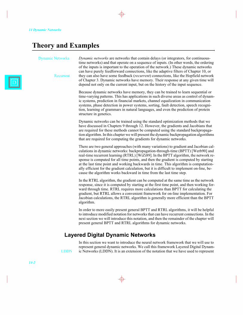
To help us introduce the LDDN notation, consider the example dynamic network given in Figure 14.1.
Figure 14.1 Example Dynamic Network
The general equations for the computation of the net input for layer m of an LDDN are
(14.1)
where is the lth input vector to the network at time t, is the input weight between input l and layer m, is the layer weight between layer l and layer m,
is the bias vector for layer m, is the set of all delays in the tapped delay line between Layer l and Layer m, is the set of all delays in the tapped delay line between Input l and Layer m, is the set of indices of input vectors that connect to layer m, and is the set of indices of layers that directly connect forward to layer m. The output of layer m is then computed as
. (14.2)
S1 x 1
S2 x 1
S3 x 1
S1 x 1
S2 x 1 S
3 x 1
S1 x 1 S
2 x 1 S3 x 1
R x 11
S1 x R S
2 x S1
S3 x S
2
S1
S2
S3
n1( )t
n2( )t n
3( )t
p1( )t
a1( )t
a2( )t a
3( )t
IW1,1
LW1,3
LW2,3
LW1,1
LW2,1
LW3,2
b1
b2
b31 1 1
R1
Inputs Layer 1 Layer 2 Layer 3
TDL
TDL
TDL
TDL
f1
f2
f3
nm t( )
nm t( ) LWm l, d( )al t d�–( )d DLm l,l Lm
f
=
IWm l, d( )pl t d�–( )d DIm l,l Im
bm+ +
pl t( ) IWm l,Input WeightLWm l,Layer Weight
bm DLm l,DIm l,Im
Lmf
am t( ) fm nm t( )( )=

14 Dynamic Networks
14-4
D
Compare this with the static multilayer network of Eq. (11.6). LDDN networks can have several layers connecting to layer m. Some of the connections can be recurrent through tapped delay lines. An LDDN can also have multiple input vectors, and the input vectors can be connected to any layer in the network; for static multilayer net-works, we assumed that the single input vector connected only to Layer 1.
With static multilayer networks, the layers were connected to each other in numerical order. In other words, Layer 1 was connected to Layer 2, which was connected to Layer 3, etc. Within the LDDN framework, any layer can connect to any other layer, even to itself. However, in order to use Eq. (14.1), we need to compute the layer outputs in a specific order. The order in which the layer outputs must be computed to obtain the correct network output is called the simulation order. (This order need not be unique; there may be several valid simulation orders.) In order to backpropagate the derivatives for the gradient calculations, we must proceed in the opposite order, which is called the backpropagation order. In Figure 14.1, the standard numerical order, 1-2-3, is the sim-ulation order, and the backpropagation order is 3-2-1.
As with the multilayer network, the fundamental unit of the LDDN is the layer. Each layer in the LDDN is made up of five components:
1. a set of weight matrices that come into that layer (which may connect from other layers or from external inputs),
2. any tapped delay lines (represented by or ) that appear at the input of a set of weight matrices (Any set of weight matrices can be preceded by a TDL. For example, Layer 1 of Figure 14.1 contains the weights and the cor-responding TDL.),
3. a bias vector,
4. a summing junction, and
5. a transfer function.
The output of the LDDN is a function not only of the weights, biases, and the current network inputs, but also of outputs of some of the network layers at previous points in time. For this reason, it is not a simple matter to calculate the gradient of the network output with respect to the weights and biases. The weights and biases have two differ-ent effects on the network output. The first is the direct effect, which can be calculated using the standard backpropagation algorithm from Chapter 11. The second is an indi-rect effect, since some of the inputs to the network are previous outputs, which are also functions of the weights and biases. The main development of the next two sections is a general gradient calculation for arbitrary LDDN�’s.
Example Dynamic NetworksBefore we introduce dynamic training, let�’s get a feeling for the types of responses we can expect to see from dynamic networks. Consider first the feedforward dynamic net-work shown in Figure 14.2.
Simulation Order
Backpropagation Order
DLm l, DIm l,
LW1 3, d( )
22+
Layered Digital Dynamic Networks
14-5
14
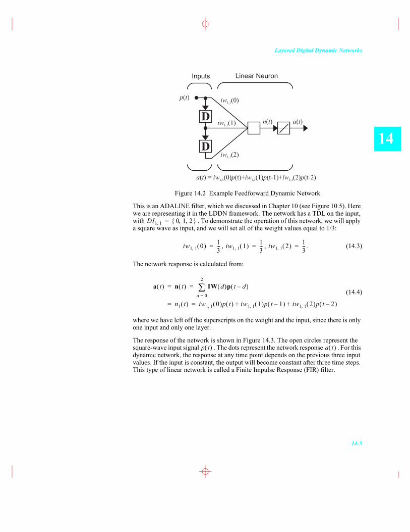
Figure 14.2 Example Feedforward Dynamic Network
This is an ADALINE filter, which we discussed in Chapter 10 (see Figure 10.5). Here we are representing it in the LDDN framework. The network has a TDL on the input, with . To demonstrate the operation of this network, we will apply a square wave as input, and we will set all of the weight values equal to 1/3:
, , . (14.3)
The network response is calculated from:
(14.4)
where we have left off the superscripts on the weight and the input, since there is only one input and only one layer.
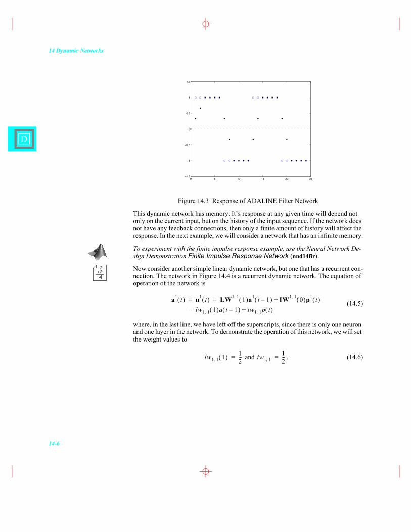
The response of the network is shown in Figure 14.3. The open circles represent the square-wave input signal . The dots represent the network response . For this dynamic network, the response at any time point depends on the previous three input values. If the input is constant, the output will become constant after three time steps. This type of linear network is called a Finite Impulse Response (FIR) filter.
iw1,1(0)
iw1,1(1)
iw1,1(2)
D
D
Inputs Linear Neuron
p t( )
n t( ) a t( )
a t( ) = )+iw p iw p iw p1,1 1,1 1,1(0) (t)+ (1) (t-1 (2) (t-2)
DI1 1, 0 1 2, ,{ }=
iw1 1, 0( ) 13---= iw1 1, 1( ) 1
3---= iw1 1, 2( ) 1
3---=
a t( ) n t( ) IW d( )p t d�–( )d 0=
2
= =
n1 t( ) iw1 1, 0( )p t( ) iw1 1, 1( )p t 1�–( ) iw1 1, 2( )p t 2�–( )+ += =
p t( ) a t( )
14 Dynamic Networks
14-6
D
Figure 14.3 Response of ADALINE Filter Network
This dynamic network has memory. It�’s response at any given time will depend not only on the current input, but on the history of the input sequence. If the network does not have any feedback connections, then only a finite amount of history will affect the response. In the next example, we will consider a network that has an infinite memory.
To experiment with the finite impulse response example, use the Neural Network De-sign Demonstration Finite Impulse Response Network (nnd14fir).
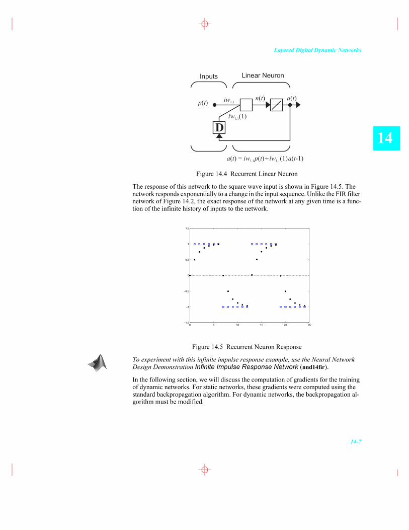
Now consider another simple linear dynamic network, but one that has a recurrent con-nection. The network in Figure 14.4 is a recurrent dynamic network. The equation of operation of the network is
(14.5)
where, in the last line, we have left off the superscripts, since there is only one neuron and one layer in the network. To demonstrate the operation of this network, we will set the weight values to
and . (14.6)
0 5 10 15 20 251.5
1
0.5
0
0.5
1
1.5
22+
a1 t( ) n1 t( ) LW1 1, 1( )a1 t 1�–( ) IW1 1, 0( )p1 t( )+= =lw1 1, 1( )a t 1�–( ) iw1 1, p t( )+=
lw1 1, 1( ) 12---= iw1 1,
12---=
Layered Digital Dynamic Networks
14-7
14
Figure 14.4 Recurrent Linear Neuron
The response of this network to the square wave input is shown in Figure 14.5. The network responds exponentially to a change in the input sequence. Unlike the FIR filter network of Figure 14.2, the exact response of the network at any given time is a func-tion of the infinite history of inputs to the network.
Figure 14.5 Recurrent Neuron Response
To experiment with this infinite impulse response example, use the Neural Network Design Demonstration Infinite Impulse Response Network (nnd14fir).
In the following section, we will discuss the computation of gradients for the training of dynamic networks. For static networks, these gradients were computed using the standard backpropagation algorithm. For dynamic networks, the backpropagation al-gorithm must be modified.
lw1,1(1)
iw1,1
D
Inputs Linear Neuron
p t( )n t( ) a t( )
a t iw p t lw a t( ) ( ) ( -1)= +1,1 1,1(1)
0 5 10 15 20 251.5
1
0.5
0
0.5
1
1.5
14 Dynamic Networks
14-8
D
Principles of Dynamic LearningBefore we get into the details of training dynamic networks, let�’s first investigate a simple example. Consider again the recurrent network of Figure 14.4. Suppose that we want to train the network using steepest descent. The first step is to compute the gra-dient of the performance function. For this example we will use sum squared error:
. (14.7)
The two elements of the gradient will be
, (14.8)
(14.9)
The key terms in these equations are the derivatives of the network output with respect to the weights:
and . (14.10)
If we had a static network, then these terms would be very easy to compute. They would correspond to and , respectively. However, for recurrent net-works, the weights have two effects on the network output. The first is the direct effect, which is also seen in the corresponding static network. The second is an indirect effect, caused by the fact that one of the network inputs is a previous network output. Let�’s compute the derivatives of the network output, in order to demonstrate these two ef-fects.
The equation of operation of the network is
. (14.11)
We can compute the terms in Eq. (14.10) by taking the derivatives of Eq. (14.11):
, (14.12)
. (14.13)
22+
F x( ) e2 t( )t 1=
Q
t t( ) a t( )�–( )2
t 1=
Q
= =
F x( )lw1 1, 1( )
------------------------ e2 t( )lw1 1, 1( )
------------------------t 1=
Q
2 e t( ) a t( )lw1 1, 1( )
------------------------t 1=
Q
�–= =
F x( )iw1 1,
--------------- e2 t( )iw1 1,
---------------t 1=
Q
2 e t( ) a t( )iw1 1,
---------------t 1=
Q
�–= =
a t( )lw1 1, 1( )
------------------------ a t( )iw1 1,
---------------
a t 1�–( ) p t( )
a t( ) lw1 1, 1( )a t 1�–( ) iw1 1, p t( )+=
a t( )lw1 1, 1( )
------------------------ a t 1�–( ) lw1 1, 1( ) a t 1�–( )lw1 1, 1( )
------------------------+=
a t( )iw1 1,
--------------- p t( ) lw1 1, 1( ) a t 1�–( )iw1 1,
----------------------+=
Principles of Dynamic Learning
14-9
14
The first term in each of these equations represents the direct effect that each weight has on the network output. The second term represents the indirect effect. Note that un-like the gradient computation for static networks, the derivative at each time point de-pends on the derivative at previous time points (or at future time points, as we will see later).
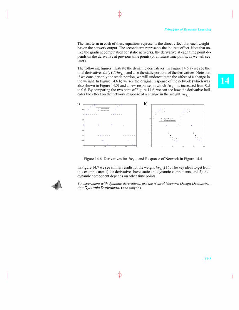
The following figures illustrate the dynamic derivatives. In Figure 14.6 a) we see the total derivatives and also the static portions of the derivatives. Note that if we consider only the static portion, we will underestimate the effect of a change in the weight. In Figure 14.6 b) we see the original response of the network (which was also shown in Figure 14.5) and a new response, in which is increased from 0.5 to 0.6. By comparing the two parts of Figure 14.6, we can see how the derivative indi-cates the effect on the network response of a change in the weight .
Figure 14.6 Derivatives for and Response of Network in Figure 14.4
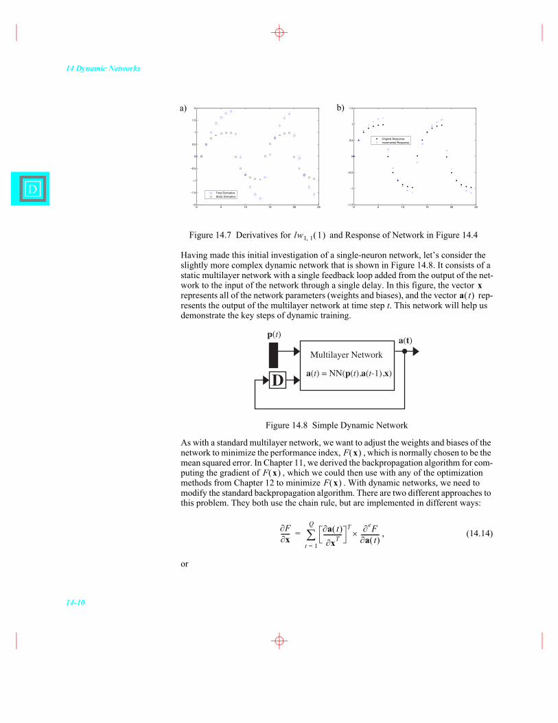
In Figure 14.7 we see similar results for the weight . The key ideas to get from this example are: 1) the derivatives have static and dynamic components, and 2) the dynamic component depends on other time points.
To experiment with dynamic derivatives, use the Neural Network Design Demonstra-tion Dynamic Derivatives (nnd14dynd).
a t( ) iw1 1,
iw1 1,
iw1 1,
0 5 10 15 20 252
1.5
1
0.5
0
0.5
1
1.5
2
Total DerivativeStatic Derivative
0 5 10 15 20 251.5
1
0.5
0
0.5
1
1.5
Original ResponseIncremental Response
a) b)
iw1 1,
lw1 1, 1( )
14 Dynamic Networks
14-10
D
Figure 14.7 Derivatives for and Response of Network in Figure 14.4
Having made this initial investigation of a single-neuron network, let�’s consider the slightly more complex dynamic network that is shown in Figure 14.8. It consists of a static multilayer network with a single feedback loop added from the output of the net-work to the input of the network through a single delay. In this figure, the vector represents all of the network parameters (weights and biases), and the vector rep-resents the output of the multilayer network at time step t. This network will help us demonstrate the key steps of dynamic training.
Figure 14.8 Simple Dynamic Network
As with a standard multilayer network, we want to adjust the weights and biases of the network to minimize the performance index, , which is normally chosen to be the mean squared error. In Chapter 11, we derived the backpropagation algorithm for com-puting the gradient of , which we could then use with any of the optimization methods from Chapter 12 to minimize . With dynamic networks, we need to modify the standard backpropagation algorithm. There are two different approaches to this problem. They both use the chain rule, but are implemented in different ways:
, (14.14)
or
0 5 10 15 20 252
1.5
1
0.5
0
0.5
1
1.5
2
Total DerivativeStatic Derivative
0 5 10 15 20 251.5
1
0.5
0
0.5
1
1.5
Original ResponseIncremental Response
a) b)
lw1 1, 1( )
xa t( )
p( )t a( )t
a( ) = NN( ( ), ( -1), )t t tp a x
Multilayer Network
D
F x( )
F x( )F x( )
Fx
------ a t( )xT------------
T eFa t( )
------------×t 1=
Q
=
Dynamic Backpropagation
14-11
14
. (14.15)
where the superscript e indicates an explicit derivative, not accounting for indirect ef-fects through time. The explicit derivatives can be obtained with the standard back-propagation algorithm of Chapter 11. To find the complete derivatives that are required in Eq. (14.14) and Eq. (14.15), we need the additional equations:
(14.16)
and
. (14.17)
Eq. (14.14) and Eq. (14.16) make up the real-time recurrent learning (RTRL) algo-rithm. Note that the key term is
, (14.18)
which must be propagated forward through time. Eq. (14.15) and Eq. (14.17) make up the backpropagation-through-time (BPTT) algorithm. Here the key term is
(14.19)
which must be propagated backward through time.
In general, the RTRL algorithm requires somewhat more computation than the BPTT algorithm to compute the gradient. However, the BPTT algorithm cannot be conve-niently implemented in real time, since the outputs must be computed for all time steps, and then the derivatives must be backpropagated back to the initial time point. The RTRL algorithm is well suited for real time implementation, since the derivatives can be calculated at each time step. (For Jacobian calculations, which are needed for Lev-enberg-Marquardt algorithms, the RTRL algorithm is often more efficient than the BPTT algorithm. See [DeHa07].)
Dynamic BackpropagationIn this section, we will develop general RTRL and BPTT algorithms for dynamic net-works represented in the LDDN framework. This development will involve generaliz-ing Eq. (14.14) through Eq. (14.17).
Fx------
ea t( )xT---------------
TF
a t( )------------×
t 1=
Q
=
a t( )xT------------
ea t( )xT---------------
ea t( )aT t 1�–( )
------------------------ a t 1�–( )
xT---------------------×+=
Fa t( )
------------eF
a t( )------------
ea t 1+( )
aT t( )------------------------ F
a t 1+( )----------------------×+=
RTRL
a t( )xT------------
BPTT
Fa t( )------------
14 Dynamic Networks
14-12
D
Preliminary DefinitionsIn order to simplify the description of the training algorithm, some layers of the LDDN will be assigned as network outputs, and some will be assigned as network inputs. A layer is an input layer if it has an input weight, or if it contains any delays with any of its weight matrices. A layer is an output layer if its output will be compared to a target during training, or if it is connected to an input layer through a matrix that has any de-lays associated with it.
For example, the LDDN shown in Figure 14.1 has two output layers (1 and 3) and two input layers (1 and 2). For this network the simulation order is 1-2-3, and the backprop-agation order is 3-2-1. As an aid in later derivations, we will define U as the set of all output layer numbers and X as the set of all input layer numbers. For the LDDN in Fig-ure 14.1, U={1,3} and X={1,2}.
The general equations for simulating an arbitrary LDDN network are given in Eq. (14.1) and Eq. (14.2). At each time point, these equations are iterated forward through the layers, as m is incremented through the simulation order. Time is then incremented from t=1 to t=Q.
Real Time Recurrent LearningIn this subsection we will generalize the RTRL algorithm, given in Eq. (14.14) and Eq. (14.16), for LDDN networks. This development will follow in many respects the de-velopment of the backpropagation algorithm for static multilayer networks in Chapter 11. You may want to quickly review that material before proceeding.
Eq. (14.14)The first step in developing the RTRL algorithm is to generalize Eq. (14.14). For the general LDDN network, we can calculate the terms of the gradient by using the chain rule, as in
. (14.20)
If we compare this equation with Eq. (14.14), we notice that in addition to each time step, we also have a term in the sum for each output layer. However, if the performance index is not explicitly a function of a specific output , then that explicit de-rivative will be zero.
Eq. (14.16)The next step of the development of the RTRL algorithm is the generalization of Eq. (14.16). Again, we use the chain rule:
. (14.21)
Input LayerOutput Layer
Fx
------ au t( )xT---------------
T eFau t( )
---------------×u Ut 1=
Q
=
F x( ) au t( )
au t( )xT---------------
eau t( )xT-----------------
eau t( )
nx t( )T-----------------
enx t( )
au' t d�–( )T---------------------------×
d DLx u',
au' t d�–( )
xT-------------------------×x Xu' U
+=
Dynamic Backpropagation
14-13
14
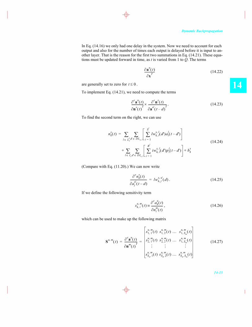
In Eq. (14.16) we only had one delay in the system. Now we need to account for each output and also for the number of times each output is delayed before it is input to an-other layer. That is the reason for the first two summations in Eq. (14.21). These equa-tions must be updated forward in time, as t is varied from 1 to Q. The terms
(14.22)
are generally set to zero for .
To implement Eq. (14.21), we need to compute the terms
. (14.23)
To find the second term on the right, we can use
(14.24)
(Compare with Eq. (11.20).) We can now write
. (14.25)
If we define the following sensitivity term
, (14.26)
which can be used to make up the following matrix
(14.27)
au t( )xT---------------
t 0
eau t( )
nx t( )T-----------------
enx t( )
au' t d�–( )T---------------------------×
nkx t( ) lwk i,
x l, d'( )ail t d'�–( )
i 1=
Sl
d' DLx l,l Lxf
=
iwk i,x l, d'( )pi
l t d'�–( )i 1=
Rl
d' DIx l,l Ix
bkx+ +
enkx t( )
aju' t d�–( )
------------------------ lwk j,x u', d( )=
sk i,u m, t( )
eaku t( )
nim t( )
-----------------
Su m, t( )eau t( )
nm t( )T-------------------
s1 1,u m, t( ) s1 2,
u m, t( ) �… s1 Sm,u m, t( )
s2 1,u m, t( ) s2 2,
u m, t( ) �… s1 Sm,u m, t( )
sSu 1,u m, t( ) sSu 2,
u m, t( ) �… sSu Sm,u m, t( )
= = �… �… �…
14 Dynamic Networks
14-14
D
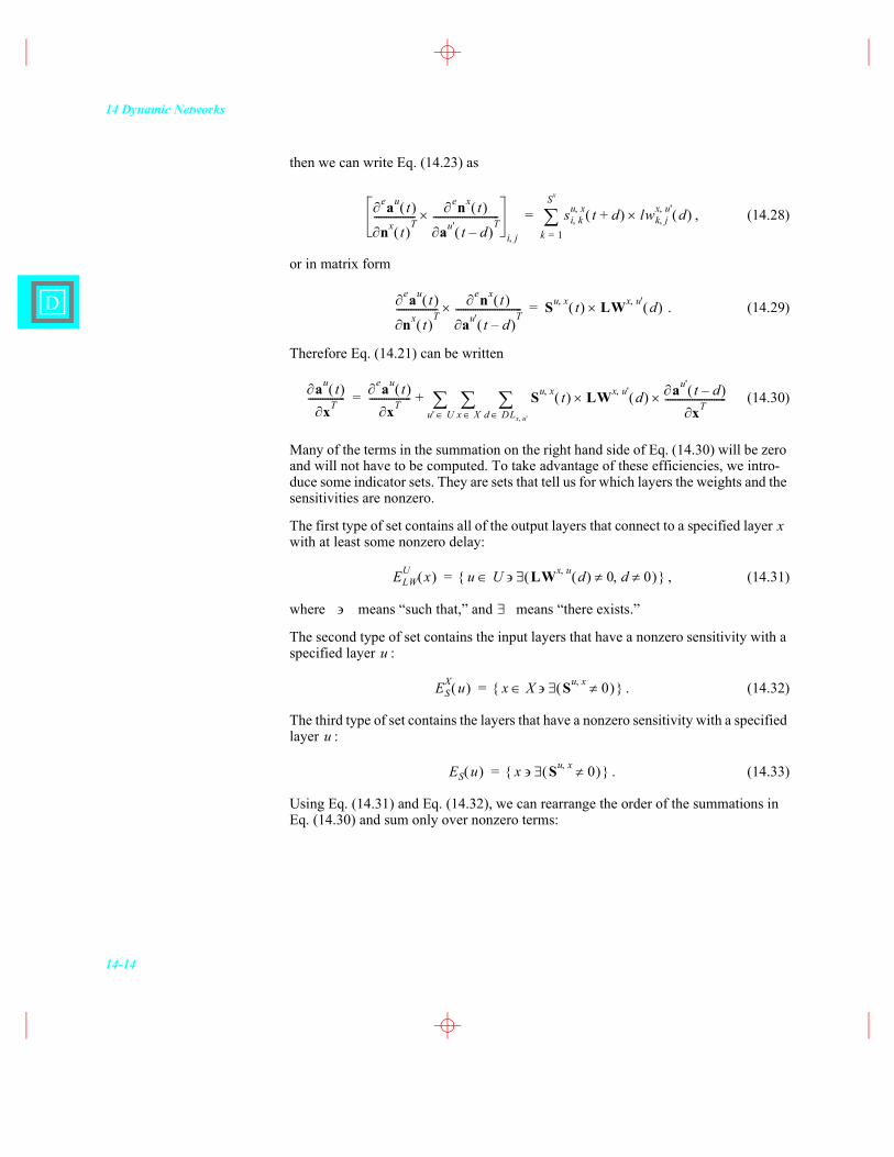
then we can write Eq. (14.23) as
, (14.28)
or in matrix form
. (14.29)
Therefore Eq. (14.21) can be written
(14.30)
Many of the terms in the summation on the right hand side of Eq. (14.30) will be zero and will not have to be computed. To take advantage of these efficiencies, we intro-duce some indicator sets. They are sets that tell us for which layers the weights and the sensitivities are nonzero.
The first type of set contains all of the output layers that connect to a specified layer with at least some nonzero delay:
, (14.31)
where means �“such that,�” and means �“there exists.�”
The second type of set contains the input layers that have a nonzero sensitivity with a specified layer :
. (14.32)
The third type of set contains the layers that have a nonzero sensitivity with a specified layer :
. (14.33)
Using Eq. (14.31) and Eq. (14.32), we can rearrange the order of the summations in Eq. (14.30) and sum only over nonzero terms:
eau t( )
nx t( )T-----------------
enx t( )
au' t d�–( )T---------------------------×
i j,
si k,u x, t d+( ) lwk j,
x u', d( )×k 1=
Sx
=
eau t( )
nx t( )T-----------------
enx t( )
au' t d�–( )T---------------------------× Su x, t( ) LWx u', d( )×=
au t( )xT---------------
eau t( )xT----------------- Su x, t( ) LWx u', d( )×
d DLx u',
au' t d�–( )
xT-------------------------×x Xu' U
+=
x
ELWU x( ) u U LWx u, d( ) 0 d 0,( ){ }=
u
ESX u( ) x X Su x, 0( ){ }=
u
ES u( ) x Su x, 0( ){ }=
Dynamic Backpropagation
14-15
14
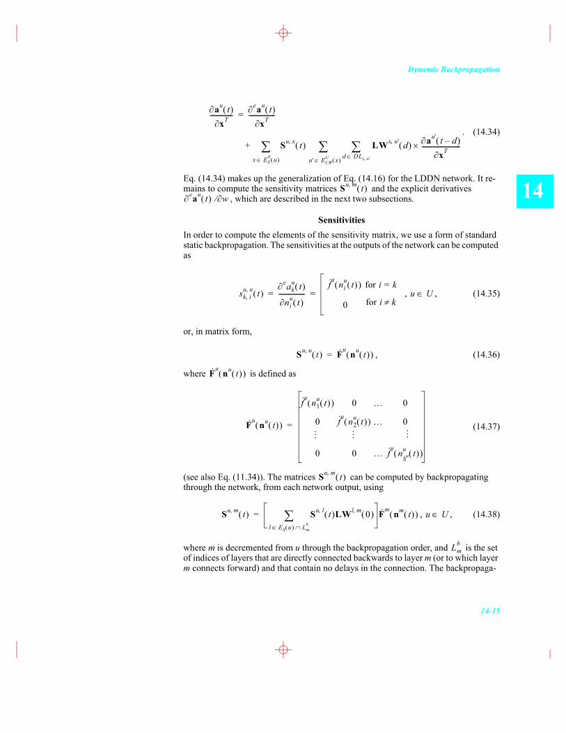
. (14.34)
Eq. (14.34) makes up the generalization of Eq. (14.16) for the LDDN network. It re-mains to compute the sensitivity matrices and the explicit derivatives
, which are described in the next two subsections.
SensitivitiesIn order to compute the elements of the sensitivity matrix, we use a form of standard static backpropagation. The sensitivities at the outputs of the network can be computed as
, , (14.35)
or, in matrix form,
, (14.36)
where is defined as
(14.37)
(see also Eq. (11.34)). The matrices can be computed by backpropagating through the network, from each network output, using
, , (14.38)
where m is decremented from u through the backpropagation order, and is the set of indices of layers that are directly connected backwards to layer m (or to which layer m connects forward) and that contain no delays in the connection. The backpropaga-
au t( )xT---------------
eau t( )xT-----------------=
Su x, t( ) LWx u', d( ) au' t d�–( )
xT-------------------------×d DLx u',u' ELW
U x( )x ESX u( )
+
Su m, t( )eau t( ) w
sk i,u u, t( )
eaku t( )
niu t( )
-----------------f·u
niu t( )( ) for i k=
0 for i k= = u U
Su u, t( ) F· u nu t( )( )=
F· u nu t( )( )
F· u nu t( )( )
f·u
n1u t( )( ) 0 �… 0
0 f·u n2u t( )( ) �… 0
0 0 �… f·u
nSuu t( )( )
= �… �… �…
Su m, t( )
Su m, t( ) Su l, t( )LWl m, 0( )l ES u( ) Lm
b
F· m nm t( )( )= u U
Lmb
14 Dynamic Networks
14-16
D
tion step given in Eq. (14.38) is essentially the same as that given in Eq. (11.45), but it is generalized to allow for arbitrary connections between layers.
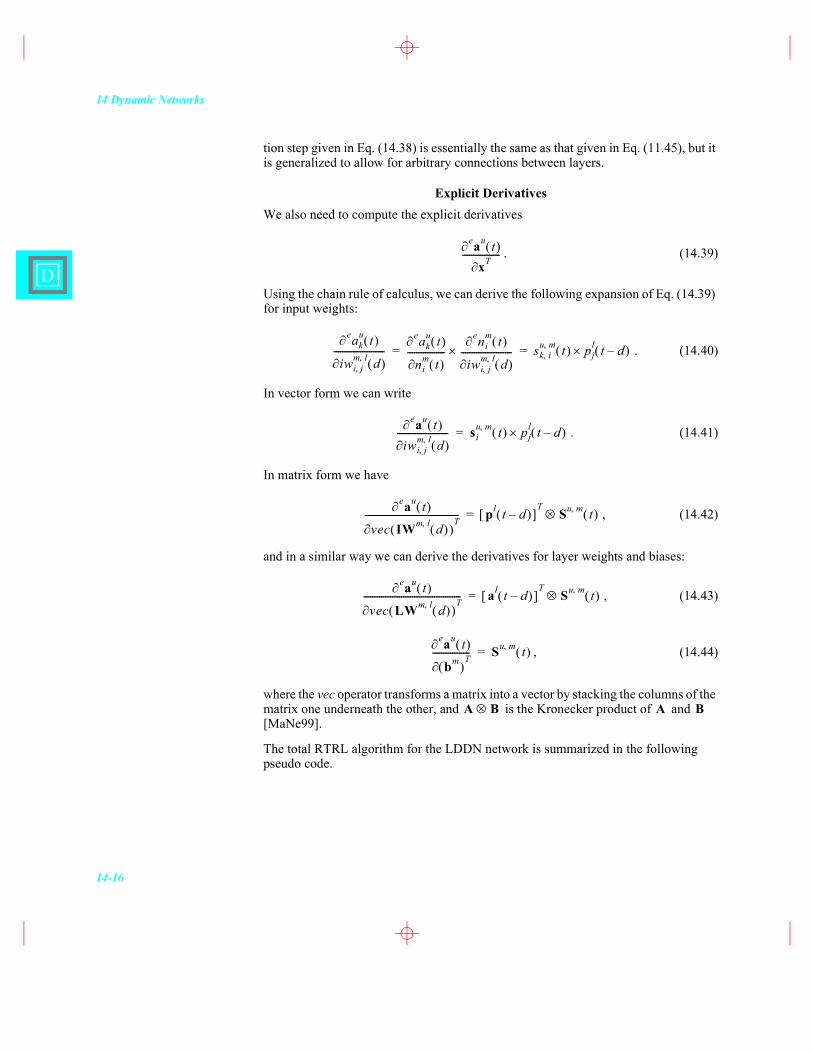
Explicit DerivativesWe also need to compute the explicit derivatives
. (14.39)
Using the chain rule of calculus, we can derive the following expansion of Eq. (14.39) for input weights:
. (14.40)
In vector form we can write
. (14.41)
In matrix form we have
, (14.42)
and in a similar way we can derive the derivatives for layer weights and biases:
, (14.43)
, (14.44)
where the vec operator transforms a matrix into a vector by stacking the columns of the matrix one underneath the other, and is the Kronecker product of and [MaNe99].
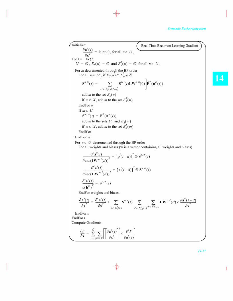
The total RTRL algorithm for the LDDN network is summarized in the following pseudo code.
eau t( )xT-----------------
eaku t( )
iwi j,m l, d( )
-----------------------eak
u t( )
nim t( )
-----------------eni
m t( )
iwi j,m l, d( )
-----------------------× sk i,u m, t( ) pj
l t d�–( )×= =
eau t( )iwi j,
m l, d( )----------------------- si
u m, t( ) pjl t d�–( )×=
eau t( )
vec IWm l, d( )( )T------------------------------------------ pl t d�–( )[ ]
TSu m, t( )=
eau t( )
vec LWm l, d( )( )T-------------------------------------------- al t d�–( )[ ]
TSu m, t( )=
eau t( )
bm( )T----------------- Su m, t( )=
A B A B
Dynamic Backpropagation
14-17
14
Initialize:
, for all ,
For t = 1 to Q,, and for all .
For m decremented through the BP orderFor all , if
add m to the set if , add m to the set
EndFor uIf
add m to the sets and if , add m to the set
EndIf mEndFor mFor decremented through the BP order
For all weights and biases (w is a vector containing all weights and biases)
EndFor weights and biases
EndFor uEndFor tCompute Gradients
au t( )xT--------------- 0 t 0,= u U
U = ES u( ) = ESX u( ) = u U
u U ES u( ) Lmb
Su m, t( ) Su l, t( )LWl m, 0( )l ES u( ) Lm
b
F· m nm t( )( )=
ES u( )m X ES
X u( )
m USm m, t( ) F· m nm t( )( )=
U ES m( )m X ES
X m( )
u U
eau t( )
vec IWm l, d( )( )T------------------------------------------ pl t d�–( )[ ]
TSu m, t( )=
eau t( )
vec LWm l, d( )( )T-------------------------------------------- al t d�–( )[ ]
TSu m, t( )=
eau t( )
bm( )T----------------- Su m, t( )=
au t( )xT---------------
eau t( )xT----------------- Su x, t( ) LWx u', d( ) au' t d�–( )
xT-------------------------×d DLx u',u' ELW
U x( )x ESX u( )
+=
Fx------ au t( )
xT---------------T eF
au t( )---------------×
u Ut 1=
Q
=
Real-Time Recurrent Learning Gradient
14 Dynamic Networks
14-18
D
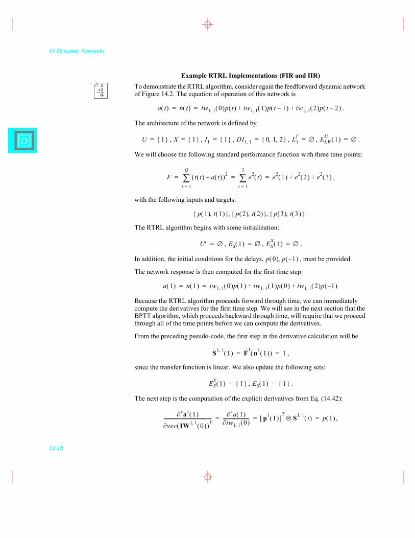
Example RTRL Implementations (FIR and IIR)To demonstrate the RTRL algorithm, consider again the feedforward dynamic network of Figure 14.2. The equation of operation of this network is
.
The architecture of the network is defined by
, , , , , .
We will choose the following standard performance function with three time points:
,
with the following inputs and targets:
.
The RTRL algorithm begins with some initialization:
, , .
In addition, the initial conditions for the delays, , must be provided.
The network response is then computed for the first time step:
Because the RTRL algorithm proceeds forward through time, we can immediately compute the derivatives for the first time step. We will see in the next section that the BPTT algorithm, which proceeds backward through time, will require that we proceed through all of the time points before we can compute the derivatives.
From the preceding pseudo-code, the first step in the derivative calculation will be
,
since the transfer function is linear. We also update the following sets:
, .
The next step is the computation of the explicit derivatives from Eq. (14.42):
,
22+
a t( ) n t( ) iw1 1, 0( )p t( ) iw1 1, 1( )p t 1�–( ) iw1 1, 2( )p t 2�–( )+ += =
U 1{ }= X 1{ }= I1 1{ }= DI1 1, 0 1 2, ,{ }= L1f = ELW
U 1( ) =
F t t( ) a t( )�–( )2
t 1=
Q
e2 t( )t 1=
3
e2 1( ) e2 2( ) e2 3( )+ += = =
p 1( ) t 1( ),{ } p 2( ) t 2( ),{ } p 3( ) t 3( ),{ }, ,
U = ES 1( ) = ESX 1( ) =
p 0( ) p 1�–( ),
a 1( ) n 1( ) iw1 1, 0( )p 1( ) iw1 1, 1( )p 0( ) iw1 1, 2( )p 1�–( )+ += =
S1 1, 1( ) F· 1 n1 1( )( ) 1= =
ESX 1( ) 1{ }= ES 1( ) 1{ }=
ea1 1( )
vec IW1 1, 0( )( )T------------------------------------------
ea 1( )iw1 1, 0( )
----------------------- p1 1( )[ ]T
S1 1, t( ) p 1( )= = =
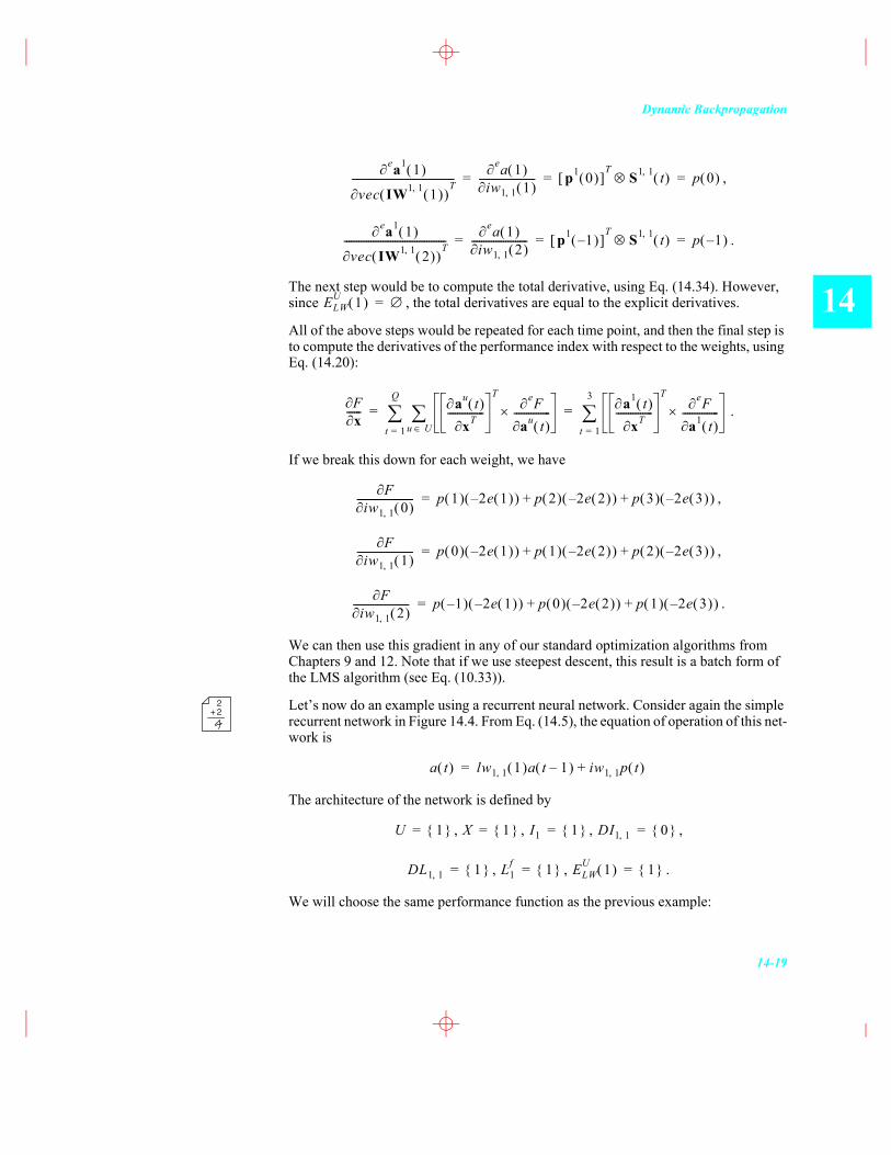
Dynamic Backpropagation
14-19
14
,
.
The next step would be to compute the total derivative, using Eq. (14.34). However, since , the total derivatives are equal to the explicit derivatives.
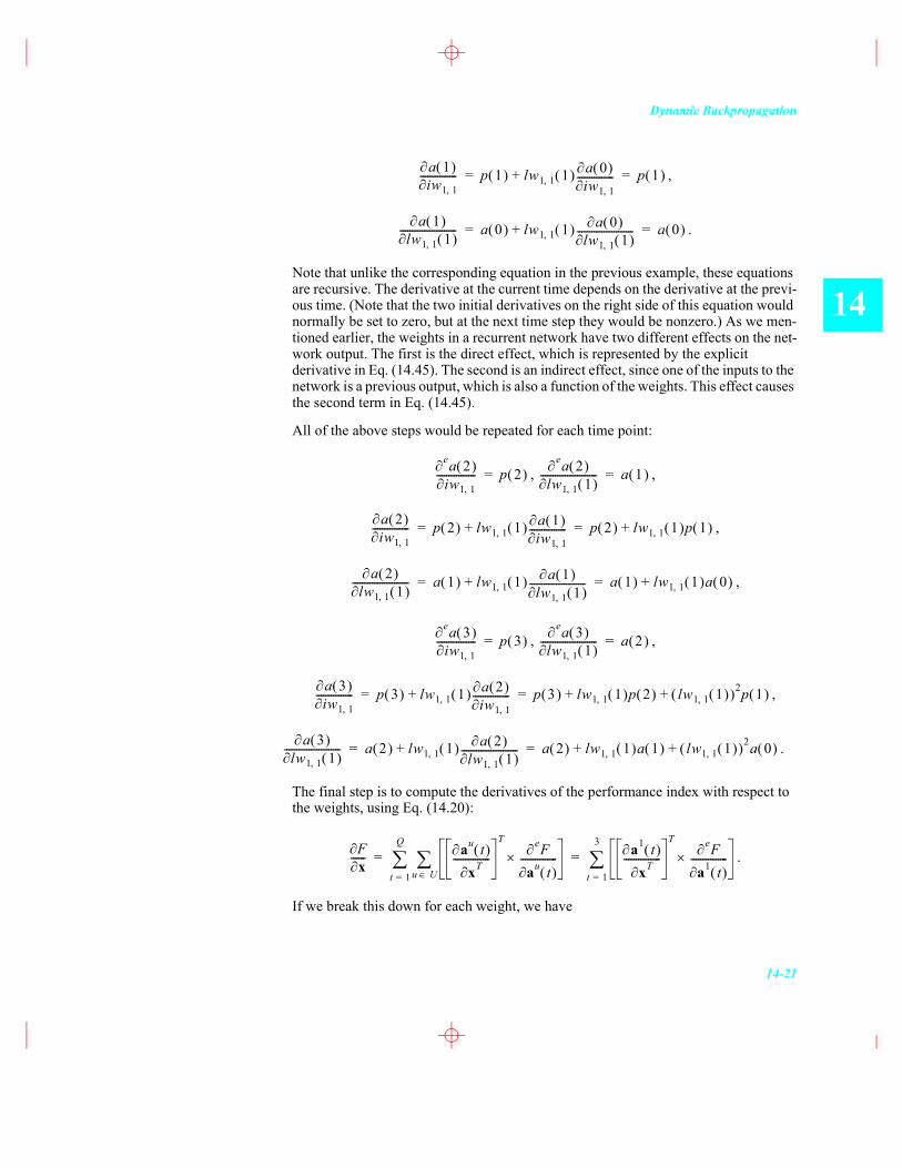
All of the above steps would be repeated for each time point, and then the final step is to compute the derivatives of the performance index with respect to the weights, using Eq. (14.20):
.
If we break this down for each weight, we have
,
,
.
We can then use this gradient in any of our standard optimization algorithms from Chapters 9 and 12. Note that if we use steepest descent, this result is a batch form of the LMS algorithm (see Eq. (10.33)).
Let�’s now do an example using a recurrent neural network. Consider again the simple recurrent network in Figure 14.4. From Eq. (14.5), the equation of operation of this net-work is
The architecture of the network is defined by
, , , ,
, , .
We will choose the same performance function as the previous example:
ea1 1( )
vec IW1 1, 1( )( )T------------------------------------------
ea 1( )iw1 1, 1( )
----------------------- p1 0( )[ ]T
S1 1, t( ) p 0( )= = =
ea1 1( )
vec IW1 1, 2( )( )T------------------------------------------
ea 1( )iw1 1, 2( )
----------------------- p1 1�–( )[ ]T
S1 1, t( ) p 1�–( )= = =
ELWU 1( ) =
Fx
------ au t( )xT---------------
T eFau t( )
---------------×u Ut 1=
Q a1 t( )xT---------------
T eFa1 t( )
---------------×t 1=
3
= =
Fiw1 1, 0( )
----------------------- p 1( ) 2e 1( )�–( ) p 2( ) 2e 2( )�–( ) p 3( ) 2e 3( )�–( )+ +=
Fiw1 1, 1( )
----------------------- p 0( ) 2e 1( )�–( ) p 1( ) 2e 2( )�–( ) p 2( ) 2e 3( )�–( )+ +=
Fiw1 1, 2( )
----------------------- p 1�–( ) 2e 1( )�–( ) p 0( ) 2e 2( )�–( ) p 1( ) 2e 3( )�–( )+ +=
22+
a t( ) lw1 1, 1( )a t 1�–( ) iw1 1, p t( )+=
U 1{ }= X 1{ }= I1 1{ }= DI1 1, 0{ }=
DL1 1, 1{ }= L1f 1{ }= ELW
U 1( ) 1{ }=
14 Dynamic Networks
14-20
D
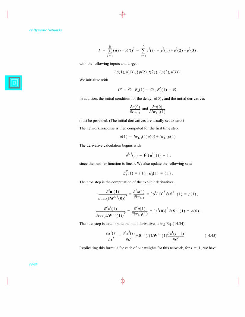
,
with the following inputs and targets:
.
We initialize with
, , .
In addition, the initial condition for the delay, , and the initial derivatives
and
must be provided. (The initial derivatives are usually set to zero.)
The network response is then computed for the first time step:
The derivative calculation begins with
,
since the transfer function is linear. We also update the following sets:
, .
The next step is the computation of the explicit derivatives:
,
.
The next step is to compute the total derivative, using Eq. (14.34):
. (14.45)
Replicating this formula for each of our weights for this network, for , we have
F t t( ) a t( )�–( )2
t 1=
Q
e2 t( )t 1=
3
e2 1( ) e2 2( ) e2 3( )+ += = =
p 1( ) t 1( ),{ } p 2( ) t 2( ),{ } p 3( ) t 3( ),{ }, ,
U = ES 1( ) = ESX 1( ) =
a 0( )
a 0( )iw1 1,
--------------- a 0( )lw1 1, 1( )
-----------------------
a 1( ) lw1 1, 1( )a 0( ) iw1 1, p 1( )+=
S1 1, 1( ) F· 1 n1 1( )( ) 1= =
ESX 1( ) 1{ }= ES 1( ) 1{ }=
ea1 1( )
vec IW1 1, 0( )( )T------------------------------------------
ea 1( )iw1 1,
---------------- p1 1( )[ ]T
S1 1, 1( ) p 1( )= = =
ea1 1( )
vec LW1 1, 1( )( )T--------------------------------------------
ea 1( )lw1 1, 1( )
----------------------- a1 0( )[ ]T
S1 1, 1( ) a 0( )= = =
a1 t( )xT---------------
ea1 t( )xT----------------- S1 1, t( )LW1 1, 1( ) a1 t 1�–( )
xT------------------------+=
t 1=
Dynamic Backpropagation
14-21
14
,
.
Note that unlike the corresponding equation in the previous example, these equations are recursive. The derivative at the current time depends on the derivative at the previ-ous time. (Note that the two initial derivatives on the right side of this equation would normally be set to zero, but at the next time step they would be nonzero.) As we men-tioned earlier, the weights in a recurrent network have two different effects on the net-work output. The first is the direct effect, which is represented by the explicit derivative in Eq. (14.45). The second is an indirect effect, since one of the inputs to the network is a previous output, which is also a function of the weights. This effect causes the second term in Eq. (14.45).
All of the above steps would be repeated for each time point:
, ,
,
,
, ,
,
.
The final step is to compute the derivatives of the performance index with respect to the weights, using Eq. (14.20):
.
If we break this down for each weight, we have
a 1( )iw1 1,
--------------- p 1( ) lw1 1, 1( ) a 0( )iw1 1,
---------------+ p 1( )= =
a 1( )lw1 1, 1( )
----------------------- a 0( ) lw1 1, 1( ) a 0( )lw1 1, 1( )
-----------------------+ a 0( )= =
ea 2( )iw1 1,
---------------- p 2( )=ea 2( )
lw1 1, 1( )----------------------- a 1( )=
a 2( )iw1 1,
--------------- p 2( ) lw1 1, 1( ) a 1( )iw1 1,
---------------+ p 2( ) lw1 1, 1( )p 1( )+= =
a 2( )lw1 1, 1( )
----------------------- a 1( ) lw1 1, 1( ) a 1( )lw1 1, 1( )
-----------------------+ a 1( ) lw1 1, 1( )a 0( )+= =
ea 3( )iw1 1,
---------------- p 3( )=ea 3( )
lw1 1, 1( )----------------------- a 2( )=
a 3( )iw1 1,
--------------- p 3( ) lw1 1, 1( ) a 2( )iw1 1,
---------------+ p 3( ) lw1 1, 1( )p 2( ) lw1 1, 1( )( )2p 1( )+ += =
a 3( )lw1 1, 1( )
----------------------- a 2( ) lw1 1, 1( ) a 2( )lw1 1, 1( )
-----------------------+ a 2( ) lw1 1, 1( )a 1( ) lw1 1, 1( )( )2a 0( )+ += =
Fx
------ au t( )xT---------------
T eFau t( )
---------------×u Ut 1=
Q a1 t( )xT---------------
T eFa1 t( )
---------------×t 1=
3
= =

14 Dynamic Networks
14-22
D
The expansions that we show in the final two lines of the above equations (and also in some of the previous equations) would not be necessary in practice. We have included them so that we can compare the result with the BPTT algorithm, which we present next.
Backpropagation-Through-TimeIn this section we will generalize the Backpropagation-Through-Time (BPTT) algo-rithm, given in Eq. (14.15) and Eq. (14.17), for LDDN networks.
Eq. (14.15)The first step is to generalize Eq. (14.15). For the general LDDN network, we can cal-culate the terms of the gradient by using the chain rule, as in
(14.46)
(for the layer weights), where u is an output layer, U is the set of all output layers, and Su is the number of neurons in layer u.
From Eq. (14.24) we can write
. (14.47)
We will also define
Fiw1 1,
--------------- a 1( )iw1 1,
--------------- 2e 1( )�–( ) a 2( )iw1 1,
--------------- 2e 2( )�–( ) a 3( )iw1 1,
--------------- 2e 3( )�–( )+ +=
2e 1( ) p 1( )[ ]�– 2e 2( ) p 2( ) lw1 1, 1( )p 1( )+[ ]�–=
2e 3( ) p 3( ) lw1 1, 1( )p 2( ) lw1 1, 1( )( )2p 1( )+ +[ ]�–
Flw1 1, 1( )
----------------------- a 1( )lw1 1, 1( )
----------------------- 2e 1( )�–( ) a 2( )lw1 1, 1( )
----------------------- 2e 2( )�–( ) a 3( )lw1 1, 1( )
----------------------- 2e 3( )�–( )+ +=
2e 1( ) a 0( )[ ]�– 2e 2( ) a 1( ) lw1 1, 1( )a 0( )+[ ]�–=
2e 3( ) a 2( ) lw1 1, 1( )a 1( ) lw1 1, 1( )( )2a 0( )+ +[ ]�–
Flwi j,
m l, d( )----------------------- F
aku t( )
---------------eak
u t( )
nim t( )
-----------------×k 1=
Su
u U
enim t( )
lwi j,m l, d( )
-----------------------t 1=
Q
=
enim t( )
lwi j,m l, d( )
----------------------- ajl t d�–( )=
Dynamic Backpropagation
14-23
14
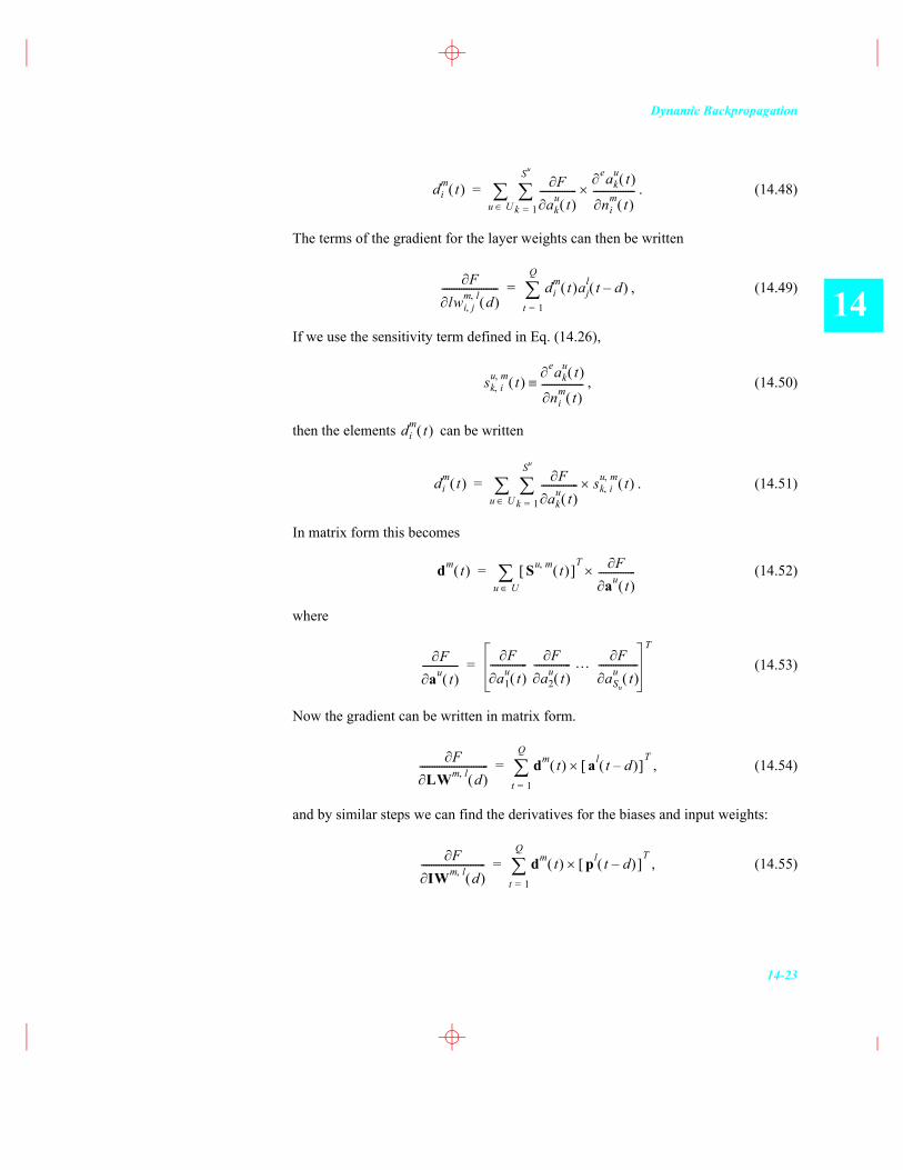
. (14.48)
The terms of the gradient for the layer weights can then be written
, (14.49)
If we use the sensitivity term defined in Eq. (14.26),
, (14.50)
then the elements can be written
. (14.51)
In matrix form this becomes
(14.52)
where
(14.53)
Now the gradient can be written in matrix form.
, (14.54)
and by similar steps we can find the derivatives for the biases and input weights:
, (14.55)
dim t( ) F
aku t( )
---------------eak
u t( )
nim t( )
-----------------×k 1=
Su
u U=
Flwi j,
m l, d( )----------------------- di
m t( )ajl t d�–( )
t 1=
Q
=
sk i,u m, t( )
eaku t( )
nim t( )
-----------------
dim t( )
dim t( ) F
aku t( )
--------------- sk i,u m, t( )×
k 1=
Su
u U=
dm t( ) Su m, t( )[ ]T F
au t( )---------------×
u U=
Fau t( )
--------------- Fa1
u t( )--------------- F
a2u t( )
--------------- �… FaSu
u t( )----------------
T
=
FLWm l, d( )
---------------------------- dm t( ) al t d�–( )[ ]T
×t 1=
Q
=
FIWm l, d( )
-------------------------- dm t( ) pl t d�–( )[ ]T
×t 1=
Q
=
14 Dynamic Networks
14-24
D
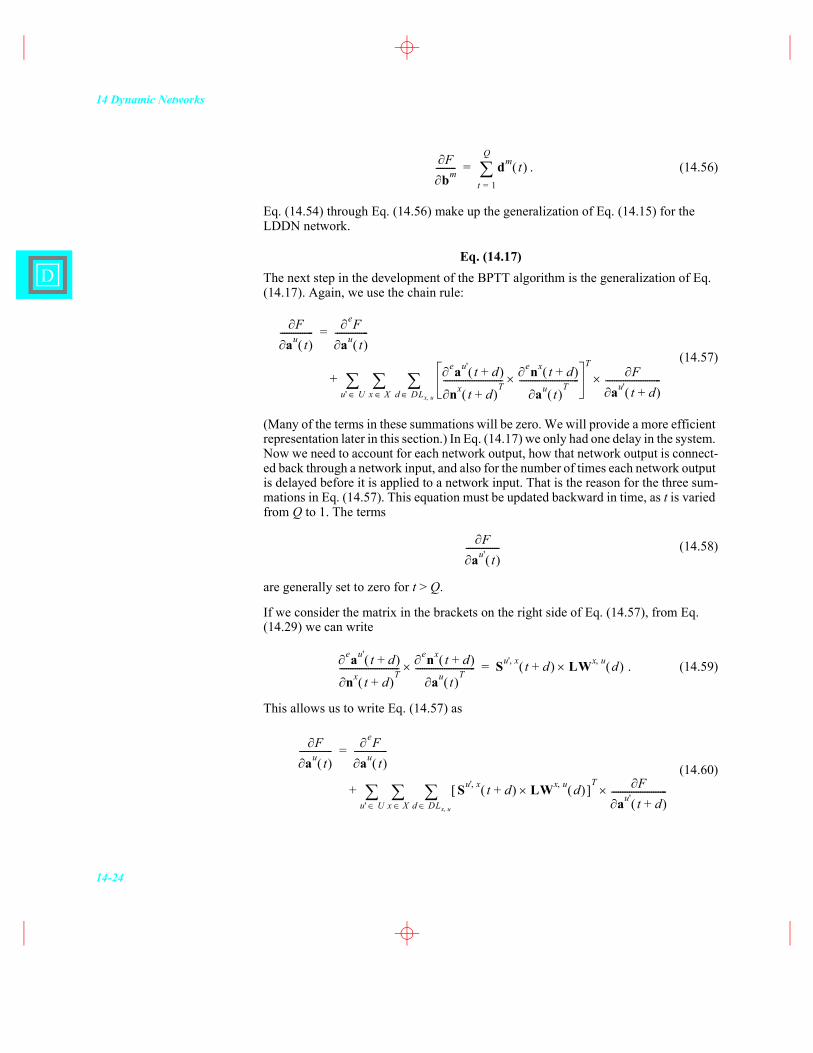
. (14.56)
Eq. (14.54) through Eq. (14.56) make up the generalization of Eq. (14.15) for the LDDN network.
Eq. (14.17)The next step in the development of the BPTT algorithm is the generalization of Eq. (14.17). Again, we use the chain rule:
(14.57)
(Many of the terms in these summations will be zero. We will provide a more efficient representation later in this section.) In Eq. (14.17) we only had one delay in the system. Now we need to account for each network output, how that network output is connect-ed back through a network input, and also for the number of times each network output is delayed before it is applied to a network input. That is the reason for the three sum-mations in Eq. (14.57). This equation must be updated backward in time, as t is varied from Q to 1. The terms
(14.58)
are generally set to zero for t > Q.
If we consider the matrix in the brackets on the right side of Eq. (14.57), from Eq. (14.29) we can write
. (14.59)
This allows us to write Eq. (14.57) as
(14.60)
Fbm--------- dm t( )
t 1=
Q
=
Fau t( )
---------------eF
au t( )---------------=
eau' t d+( )
nx t d+( )T---------------------------
enx t d+( )
au t( )T---------------------------×
TF
au' t d+( )-------------------------×
d DLx u,x Xu' U+
Fau' t( )
---------------
eau' t d+( )
nx t d+( )T---------------------------
enx t d+( )
au t( )T---------------------------× Su' x, t d+( ) LWx u, d( )×=
Fau t( )
---------------eF
au t( )---------------=
Su' x, t d+( ) LWx u, d( )×[ ]T F
au' t d+( )-------------------------×
d DLx u,x Xu' U+

Dynamic Backpropagation
14-25
14
Many of the terms in the summation on the right hand side of Eq. (14.60) will be zero and will not have to be computed. In order to provide a more efficient implementation of Eq. (14.60), we define the following sets:
, (14.61)
. (14.62)
We can now rearrange the order of the summation in Eq. (14.60) and sum only over the existing terms:
(14.63)
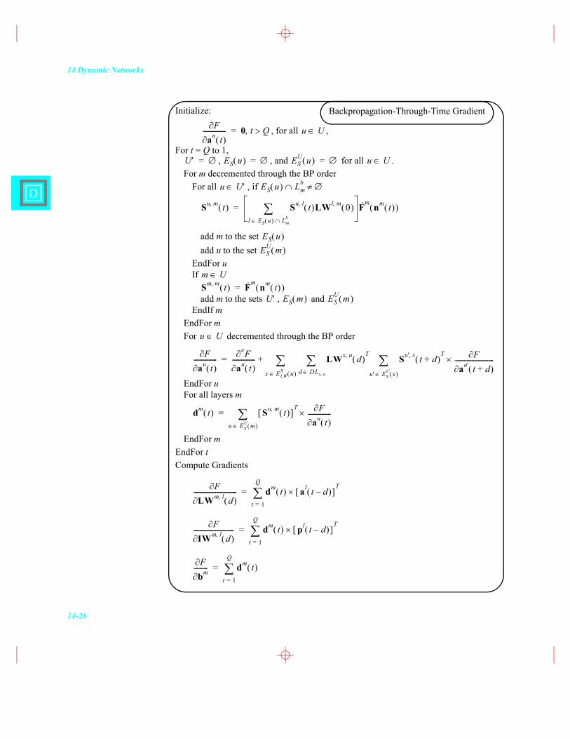
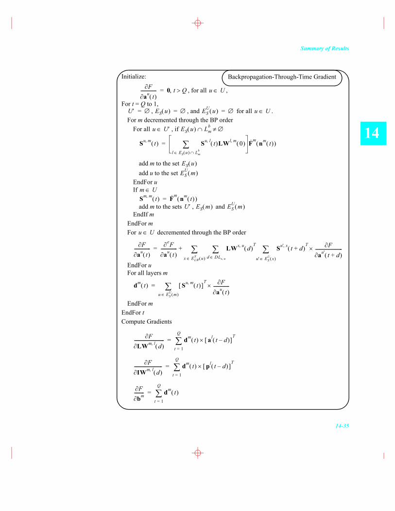
SummaryThe total BPTT algorithm is summarized in the following pseudo code.
ELWX u( ) x X LWx u, d( ) 0 d 0,( ){ }=
ESU x( ) u U Su x, 0( ){ }=
Fau t( )
---------------eF
au t( )---------------=
LWx u, d( )T
Su' x, t d+( )T F
au' t d+( )-------------------------×
u' ESU x( )d DLx u,x ELW
X u( )
+
14 Dynamic Networks
14-26
D
Initialize:
, for all ,
For t = Q to 1,, , and for all .
For m decremented through the BP orderFor all , if
add m to the set add u to the set
EndFor uIf
add m to the sets , and EndIf m
EndFor mFor decremented through the BP order
EndFor uFor all layers m
EndFor mEndFor tCompute Gradients
Fau t( )
--------------- 0 t Q>,= u U
U = ES u( ) = ESU u( ) = u U
u U ES u( ) Lmb
Su m, t( ) Su l, t( )LWl m, 0( )l ES u( ) Lm
b
F· m nm t( )( )=
ES u( )ES
U m( )
m USm m, t( ) F· m nm t( )( )=
U ES m( ) ESU m( )
u U
Fau t( )
---------------eF
au t( )--------------- LWx u, d( )
TSu' x, t d+( )
T Fau' t d+( )
-------------------------×u' ES
U x( )d DLx u,x ELWX u( )
+=
dm t( ) Su m, t( )[ ]T F
au t( )---------------×
u ESU m( )
=
FLWm l, d( )
---------------------------- dm t( ) al t d�–( )[ ]T
×t 1=
Q
=
FIWm l, d( )
-------------------------- dm t( ) pl t d�–( )[ ]T
×t 1=
Q
=
Fbm--------- dm t( )
t 1=
Q
=
Backpropagation-Through-Time Gradient
Dynamic Backpropagation
14-27
14
Example BPTT Implementations (FIR and IIR)To demonstrate the BPTT algorithm, we will use the same example networks that we used for the RTRL algorithm. First, we use the feedforward dynamic network of Figure 14.2. We defined the network architecture on page 14-18.
Before the gradient can be computed using BPTT, the network response must be com-puted for all time steps:
,
,
.
The BPTT algorithm begins with some initialization:
, , .
The first step in the derivative calculation will be the sensitivity calculation. For BPTT, we start at the last time point ( ):
,
since the transfer function is linear. We also update the following sets:
, .
The next step is the calculation of the following derivative using Eq. (14.63):
.
The final step for is Eq. (14.52):
.
We repeat the previous steps for and , to obtain
,
.
Now, all time steps are combined in Eq. (14.55):
22+
a 1( ) n 1( ) iw1 1, 0( )p 1( ) iw1 1, 1( )p 0( ) iw1 1, 2( )p 1�–( )+ += =
a 2( ) n 2( ) iw1 1, 0( )p 2( ) iw1 1, 1( )p 1( ) iw1 1, 2( )p 0( )+ += =
a 3( ) n 3( ) iw1 1, 0( )p 3( ) iw1 1, 2( )p 0( ) iw1 1, 2( )p 1( )+ += =
U = ES 1( ) = ESU 1( ) =
t 3=
S1 1, 3( ) F· 1 n1 3( )( ) 1= =
ESU 1( ) 1{ }= ES 1( ) 1{ }=
Fa1 3( )
----------------eF
a1 3( )---------------- 2e 3( )�–= =
t 3=
d1 3( ) S1 1, 3( )[ ]T F
a1 3( )----------------× 2e 3( )�–= =
t 2= t 1=
d1 2( ) S1 1, 2( )[ ]T F
a1 2( )----------------× 2e 2( )�–= =
d1 1( ) S1 1, 1( )[ ]T F
a1 1( )----------------× 2e 1( )�–= =
14 Dynamic Networks
14-28
D
,
,
.
Note that this is the same result we obtained for the RTRL algorithm example on page 14-19. RTRL and BPTT should always produce the same gradient. The only difference is in the implementation.
Let�’s now use our previous recurrent neural network example of Figure 14.4. We de-fined the architecture of this network on page 14-19.
Unlike the RTRL algorithm, where initial conditions for the derivatives must be pro-vided, the BPTT algorithm requires final conditions for the derivatives:
and ,
which are normally set to zero.
The network response is then computed for all time steps:
The derivative calculation begins with
,
since the transfer function is linear. We also update the following sets:
, .
Next we compute the following derivative using Eq. (14.63):
FIW1 1, 0( )
-------------------------- Fiw1 1, 0( )
----------------------- d1 t( ) p1 t( )[ ]T
×t 1=
3
2e t( )�– p t( )×t 1=
3
= = =
FIW1 1, 1( )
-------------------------- Fiw1 1, 1( )
----------------------- d1 t( ) p1 t 1�–( )[ ]T
×t 1=
3
2e t( )�– p t 1�–( )×t 1=
3
= = =
FIW1 1, 2( )
-------------------------- Fiw1 1, 2( )
----------------------- d1 t( ) p1 t 2�–( )[ ]T
×t 1=
3
2e t( )�– p t 2�–( )×t 1=
3
= = =
22+
a 4( )iw1 1,
--------------- a 4( )lw1 1, 1( )
-----------------------
a 1( ) lw1 1, 1( )a 0( ) iw1 1, p 1( )+=
a 2( ) lw1 1, 1( )a 1( ) iw1 1, p 2( )+=
a 3( ) lw1 1, 1( )a 2( ) iw1 1, p 3( )+=
S1 1, 3( ) F· 1 n1 3( )( ) 1= =
ESX 1( ) 1{ }= ES 1( ) 1{ }=
Dynamic Backpropagation
14-29
14
For , we find
and
Continuing to ,
,
and
Finally, for ,
,
and
Now we can compute the total gradient, using Eq. (14.54) and Eq. (14.55):
Fa1 t( )
---------------eF
a1 t( )--------------- LW1 1, 1( )
TS1 1, t 1+( )
T Fa1 t 1+( )
------------------------×+=
t 3=
Fa1 3( )
----------------eF
a1 3( )---------------- lw1 1, 1( )S1 1, 4( )
T Fa1 4( )
----------------×+eF
a1 3( )---------------- 2e 3( )�–= = =
0
d1 3( ) S1 1, 3( )[ ]T F
a1 3( )----------------× 2e 3( )�–= =
t 2=
S1 1, 2( ) F· 1 n1 2( )( ) 1= =
Fa1 2( )
----------------eF
a1 2( )---------------- lw1 1, 1( )S1 1, 3( )
T Fa1 3( )
----------------×+=
2e 2( )�– lw1 1, 1( ) 2e 3( )�–( )+=
d1 2( ) S1 1, 2( )[ ]T F
a1 2( )----------------× 2e 2( )�– lw1 1, 1( ) 2e 3( )�–( )+= =
t 1=
S1 1, 1( ) F· 1 n1 1( )( ) 1= =
Fa1 1( )
----------------eF
a1 1( )---------------- lw1 1, 1( )S1 1, 2( )
T Fa1 2( )
----------------×+=
2e 1( )�– lw1 1, 1( ) 2e 2( )�–( ) lw1 1, 1( )( )2 2e 3( )�–( )+ +=
d1 1( ) S1 1, 1( )[ ]T F
a1 1( )----------------× 2e 1( )�– lw1 1, 1( ) 2e 2( )�–( ) lw1 1, 1( )( )2 2e 3( )�–( )+ += =
14 Dynamic Networks
14-30
D
This is the same result that we obtained with the RTRL algorithm on page 14-21.
Summary and Comments on Dynamic TrainingThe RTRL and BPTT algorithms represent two methods for computing the gradients for dynamic networks. Both algorithms compute the exact gradient, and therefore they produce the same final results. The RTRL algorithm performs the calculations from the first time point forward, which is suitable for on-line (real-time) implementation. The BPTT algorithm starts from the last time point and works backward in time. The BPTT algorithm generally requires fewer computations for the gradient calculation than RTRL, but BPTT usually requires more memory storage.
In addition to the gradient, versions of BPTT and RTRL can be used to compute Jaco-bian matrices, as are needed in the Levenberg-Marquardt described in Chapter 12. For Jacobian calculations, the RTRL algorithm is generally more efficient that the BPTT algorithm. See [DeHa07] for details.
Once the gradients or Jacobians are computed, many standard optimization algorithms can be used to train the networks. However, training dynamic networks is generally more difficult than training feedforward networks - for a number of reasons. First, a recurrent net can be thought of as a feedforward network, in which the recurrent net-work is unfolded in time. For example, consider the simple single-layer recurrent net-work of Figure 14.4. If this network were to be trained over five time steps, we could unfold the network to create 5 layers - one for each time step. If a sigmoid transfer function is used, then if the output of the network is near the saturation point for any time point, the resulting gradient could be quite small.
Another problem in training dynamic networks is the shape of the error surface. It has been shown (see [DeHo01]) that the error surfaces of recurrent networks can have spu-rious valleys that are not related to the functional that is being approximated. The un-derlying cause of these valleys is the fact that recurrent networks have the potential for instabilities. For example, the network of Figure 14.4 will be unstable if is greater than one in magnitude. However, it is possible, for a particular input sequence,
FLW1 1, 1( )
---------------------------- Flw1 1, 1( )
----------------------- d1 t( ) a1 t 1�–( )[ ]T
×t 1=
3
= =
a 0( ) 2e 1( )�– lw1 1, 1( ) 2e 2( )�–( ) lw1 1, 1( )( )2 2e 3( )�–( )+ +[ ]=
a 1( ) 2e 2( )�– lw1 1, 1( ) 2e 3( )�–( )+[ ] a 0( ) 2e 3( )�–[ ]+ +
FIW1 1, 0( )
-------------------------- Fiw1 1,
--------------- d1 t( ) p1 t( )[ ]T
×t 1=
3
= =
p 1( ) 2e 1( )�– lw1 1, 1( ) 2e 2( )�–( ) lw1 1, 1( )( )2 2e 3( )�–( )+ +[ ]=
p 2( ) 2e 2( )�– lw1 1, 1( ) 2e 3( )�–( )+[ ] p 3( ) 2e 3( )�–[ ]+ +
lw1 1, 1( )
Dynamic Backpropagation
14-31
14
that the network output can be small for a particular value of greater than one in magnitude, or for certain combinations of values for and .
Finally, it is sometimes difficult to get adequate training data for dynamic networks. This is because the inputs to some layers will come from tapped delay lines. This means that the elements of the input vector cannot be selected independently, since the time sequence from which they are sampled is generally correlated in time. Unlike stat-ic networks, in which the network response depends only on the input to the network at the current time, dynamic network responses depend on the history of the input se-quence. The data used to train the network must be representative of all situations for which the network will be used, both in terms of the ranges for each input, but also in terms of the variation of the inputs over time.
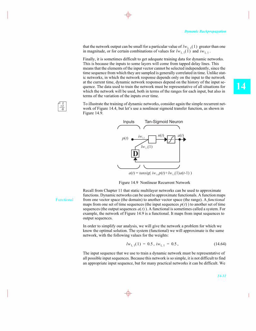
To illustrate the training of dynamic networks, consider again the simple recurrent net-work of Figure 14.4, but let�’s use a nonlinear sigmoid transfer function, as shown in Figure 14.9.
Figure 14.9 Nonlinear Recurrent Network
Recall from Chapter 11 that static multilayer networks can be used to approximate functions. Dynamic networks can be used to approximate functionals. A function maps from one vector space (the domain) to another vector space (the range). A functional maps from one set of time sequences (the input sequences ) to another set of time sequences (the output sequences ). A functional is sometimes called a system. For example, the network of Figure 14.9 is a functional. It maps from input sequences to output sequences.
In order to simplify our analysis, we will give the network a problem for which we know the optimal solution. The system (functional) we will approximate is the same network, with the following values for the weights:
, , (14.64)
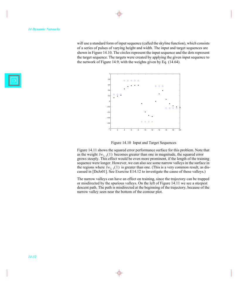
The input sequence that we use to train a dynamic network must be representative of all possible input sequences. Because this network is so simple, it is not difficult to find an appropriate input sequence, but for many practical networks it can be difficult. We
lw1 1, 1( )lw1 1, 1( ) iw1 1,
22+
lw1,1(1)
iw1,1
D
Inputs Tan-Sigmoid Neuron
p t( )n t( ) a t( )
a t iw p t lw a t( ) ( ) (1) ( -1) )= ( +tansig 1,1 1,1
Functionalp t( )
a t( )
lw1 1, 1( ) 0.5= iw1 1, 0.5=
14 Dynamic Networks
14-32
D
will use a standard form of input sequence (called the skyline function), which consists of a series of pulses of varying height and width. The input and target sequences are shown in Figure 14.10. The circles represent the input sequence and the dots represent the target sequence. The targets were created by applying the given input sequence to the network of Figure 14.9, with the weights given by Eq. (14.64).
Figure 14.10 Input and Target Sequences
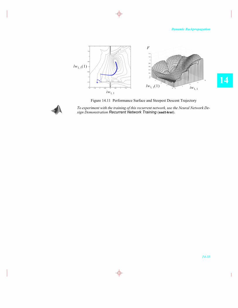
Figure 14.11 shows the squared error performance surface for this problem. Note that as the weight becomes greater than one in magnitude, the squared error grows steeply. This effect would be even more prominent, if the length of the training sequence were longer. However, we can also see some narrow valleys in the surface in the regions where is greater than one. (This is a very common result, as dis-cussed in [DeJo01]. See Exercise E14.12 to investigate the cause of these valleys.)
The narrow valleys can have an effect on training, since the trajectory can be trapped or misdirected by the spurious valleys. On the left of Figure 14.11 we see a steepest descent path. The path is misdirected at the beginning of the trajectory, because of the narrow valley seen near the bottom of the contour plot.
0 2 4 6 8 10 12 14 16 18 201
0.8
0.6
0.4
0.2
0
0.2
0.4
0.6
0.8
1
lw1 1, 1( )
lw1 1, 1( )
Dynamic Backpropagation
14-33
14
Figure 14.11 Performance Surface and Steepest Descent Trajectory
To experiment with the training of this recurrent network, use the Neural Network De-sign Demonstration Recurrent Network Training (nnd14rnt).
21
01
2
2
1
0
1
2
0
0.2
0.4
0.6
0.8
1
1.2
1.4
2 1.5 1 0.5 0 0.5 1 1.5 22
1.5
1
0.5
0
0.5
1
1.5
2
lw1 1, 1( ) iw1 1,
F
lw1 1, 1( )
iw1 1,
14 Dynamic Networks
14-34
D
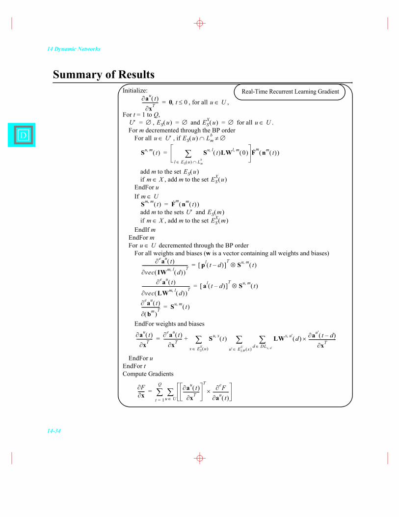
Summary of ResultsInitialize:
, for all ,
For t = 1 to Q,, and for all .
For m decremented through the BP orderFor all , if
add m to the set if , add m to the set
EndFor uIf
add m to the sets and if , add m to the set
EndIf mEndFor mFor decremented through the BP order
For all weights and biases (w is a vector containing all weights and biases)
EndFor weights and biases
EndFor uEndFor tCompute Gradients
au t( )xT--------------- 0 t 0,= u U
U = ES u( ) = ESX u( ) = u U
u U ES u( ) Lmb
Su m, t( ) Su l, t( )LWl m, 0( )l ES u( ) Lm
b
F· m nm t( )( )=
ES u( )m X ES
X u( )
m USm m, t( ) F· m nm t( )( )=
U ES m( )m X ES
X m( )
u U
eau t( )
vec IWm l, d( )( )T------------------------------------------ pl t d�–( )[ ]
TSu m, t( )=
eau t( )
vec LWm l, d( )( )T-------------------------------------------- al t d�–( )[ ]
TSu m, t( )=
eau t( )
bm( )T----------------- Su m, t( )=
au t( )xT---------------
eau t( )xT----------------- Su x, t( ) LWx u', d( ) au' t d�–( )
xT-------------------------×d DLx u',u' ELW
U x( )x ESX u( )
+=
Fx------ au t( )
xT---------------T eF
au t( )---------------×
u Ut 1=
Q
=
Real-Time Recurrent Learning Gradient
Summary of Results
14-35
14
Initialize:
, for all ,
For t = Q to 1,, , and for all .
For m decremented through the BP orderFor all , if
add m to the set add u to the set
EndFor uIf
add m to the sets , and EndIf m
EndFor mFor decremented through the BP order
EndFor uFor all layers m
EndFor mEndFor tCompute Gradients
Fau t( )
--------------- 0 t Q>,= u U
U = ES u( ) = ESU u( ) = u U
u U ES u( ) Lmb
Su m, t( ) Su l, t( )LWl m, 0( )l ES u( ) Lm
b
F· m nm t( )( )=
ES u( )ES
U m( )
m USm m, t( ) F· m nm t( )( )=
U ES m( ) ESU m( )
u U
Fau t( )
---------------eF
au t( )--------------- LWx u, d( )
TSu' x, t d+( )
T Fau' t d+( )
-------------------------×u' ES
U x( )d DLx u,x ELWX u( )
+=
dm t( ) Su m, t( )[ ]T F
au t( )---------------×
u ESU m( )
=
FLWm l, d( )
---------------------------- dm t( ) al t d�–( )[ ]T
×t 1=
Q
=
FIWm l, d( )
-------------------------- dm t( ) pl t d�–( )[ ]T
×t 1=
Q
=
Fbm--------- dm t( )
t 1=
Q
=
Backpropagation-Through-Time Gradient

14 Dynamic Networks
14-36
D
Definitions/Notation is the lth input vector to the network at time t.
is the net input for layer m.
is the transfer function for layer m.
is the output for layer m.
is the input weight between input l and layer m.
is the layer weight between layer l and layer m.
is the bias vector for layer m.
is the set of all delays in the tapped delay line between Layer l and Layer m.
is the set of all delays in the tapped delay line between Input l and Layer m.
is the set of indices of input vectors that connect to layer m.
is the set of indices of layers that directly connect forward to layer m.
is the set of indices of layers that are directly connected backwards to layer m (or to which layer m connects forward) and that contain no delays in the connection.
A layer is an input layer if it has an input weight, or if it contains any delays with any of its weight matrices. The set of input layers is X.
A layer is an output layer if its output will be compared to a target during training, or if it is connected to an input layer through a matrix that has any delays associated with it. The set of output layers is U.
The sensitivity is defined .
pl t( )
nm t( )
fm( )
am t( )
IWm l,
LWm l,
bm
DLm l,
DIm l,
Im
Lmf
Lmb
sk i,u m, t( )
eaku t( )
nim t( )
-----------------
ELWU x( ) u U LWx u, d( ) 0 d 0,( ){ }=
ESX u( ) x X Su x, 0( ){ }=
ES u( ) x Su x, 0( ){ }=
ELWX u( ) x X LWx u, d( ) 0 d 0,( ){ }=
ESU x( ) u U Su x, 0( ){ }=
Solved Problems
14-37
14
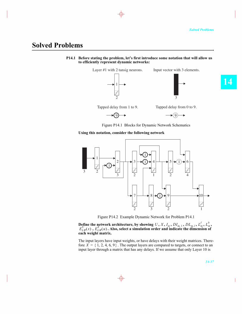
Solved ProblemsP14.1 Before stating the problem, let�’s first introduce some notation that will allow us
to efficiently represent dynamic networks:
Figure P14.1 Blocks for Dynamic Network Schematics
Using this notation, consider the following network
Figure P14.2 Example Dynamic Network for Problem P14.1
Define the network architecture, by showing , , , , , , , , . Also, select a simulation order and indicate the dimension of
each weight matrix.
The input layers have input weights, or have delays with their weight matrices. There-fore . The output layers are compared to targets, or connect to an input layer through a matrix that has any delays. If we assume that only Layer 10 is
99
32
1
Layer #1 with 2 tansig neurons. Input vector with 3 elements.
Tapped delay from 1 to 9. Tapped delay from 0 to 9.
11 1
1
1
3 22
2
1
3
2
2
4
1
3
13
7
4
8
5
9
6
10
2
U X Im DIm 1, DLm l, Lmf Lm
b
ELWU x( ) ELW
X u( )
X 1 2 4 6 9, , , ,{ }=
14 Dynamic Networks
14-38
D
compared to a target, then . Since the single input vector con-nects only to Layer 1, the only nonempty set of inputs will be . For the same reason, there will only be one nonempty set of input delays: . The con-nections between layers are defined by
, , , , ,
, , , , .
, , , , ,
, , , , .
Associated with these connections are the following layer delays
, , , , ,
, , , , ,
, , , , .
The layers that have connections from output layers are
, ,
, .
The layers that connect to input layers are
, , ,
, .
The simulation order can be chosen to be . The dimen-sions of the weight matrices are
, , , ,
, , , ,
, , , ,
, , , .
U 2 3 4 5 8 10, , , , ,{ }=I1 1{ }=DI1 1, 0{ }=
L1f = L2
f 1 2,{ }= L3f 2{ }= L4
f 3 4 7, ,{ }= L5f 4{ }=
L6f 2 5,{ }= L7
f 2{ }= L8f 7{ }= L9
f 4 8,{ }= L10f 6 9,{ }=
L1b 2{ }= L2
b 3 6 7, ,{ }= L3b = L4
b 5 9,{ }= L5b =
L6b 10{ }= L7
b 4 8,{ }= L8b = L9
b 10{ }= L10b =
DL2 1, 0{ }= DL2 2, 1{ }= DL3 2, 0{ }= DL4 3, 1{ }= DL4 4, 1{ }=
DL4 7, 0{ }= DL5 4, 0{ }= DL6 2, 0{ }= DL6 5, 0 1,{ }= DL7 2, 0{ }=
DL8 7, 0{ }= DL9 4, 0{ }= DL9 8, 1{ }= DL10 6, 0{ }= DL10 9, 0{ }=
ELWU 2( ) 2{ }= ELW
U 4( ) 3 4,{ }=
ELWU 6( ) 5{ }= ELW
U 9( ) 8{ }=
ELWX 2( ) 2{ }= ELW
X 3( ) 4{ }= ELWX 4( ) 4{ }=
ELWX 5( ) 6{ }= ELW
X 8( ) 9{ }=
1 2 3 7 4 5 6 8 9 10, , , , , , , , ,{ }
IW1 1, 0( ) 2 3× LW2 1, 0( ) 3 2× LW2 2, 1( ) 3 3× LW3 2, 0( ) 2 3×
LW4 3, 1( ) 1 2× LW4 4, 1( ) 1 1× LW4 7, 0( ) 1 2× LW5 4, 0( ) 2 1×
LW6 2, 0( ) 4 3× LW6 5, 1( ) 4 2× LW7 2, 0( ) 2 3× LW8 7, 0( ) 3 2×
LW9 4, 0( ) 2 1× LW9 8, 1( ) 2 3× LW10 6, 0( ) 1 4× LW10 9, d( ) 1 2×
Solved Problems
14-39
14
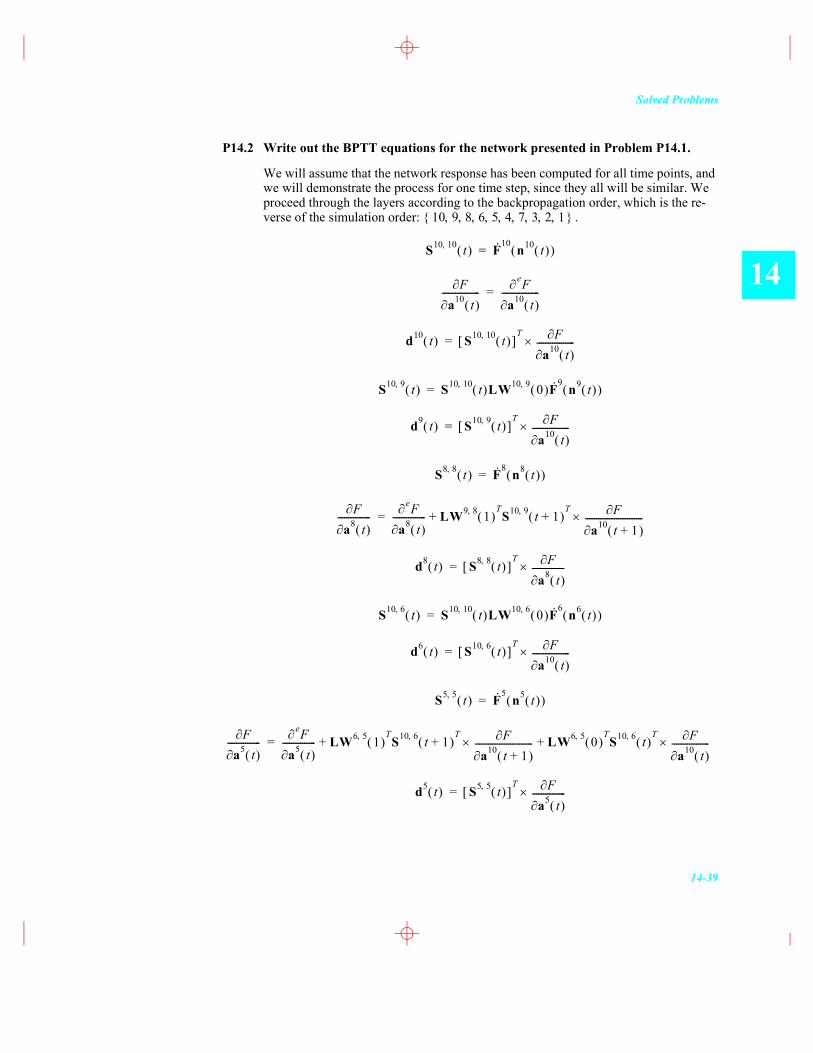
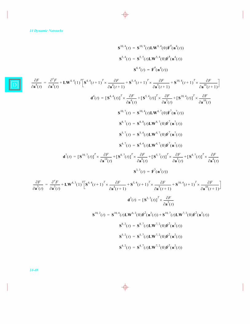
P14.2 Write out the BPTT equations for the network presented in Problem P14.1.
We will assume that the network response has been computed for all time points, and we will demonstrate the process for one time step, since they all will be similar. We proceed through the layers according to the backpropagation order, which is the re-verse of the simulation order: .10 9 8 6 5 4 7 3 2 1, , , , , , , , ,{ }
S10 10, t( ) F· 10 n10 t( )( )=
Fa10 t( )
-----------------eF
a10 t( )-----------------=
d10 t( ) S10 10, t( )[ ]T F
a10 t( )-----------------×=
S10 9, t( ) S10 10, t( )LW10 9, 0( )F· 9 n9 t( )( )=
d9 t( ) S10 9, t( )[ ]T F
a10 t( )-----------------×=
S8 8, t( ) F· 8 n8 t( )( )=
Fa8 t( )
---------------eF
a8 t( )--------------- LW9 8, 1( )
TS10 9, t 1+( )
T Fa10 t 1+( )
--------------------------×+=
d8 t( ) S8 8, t( )[ ]T F
a8 t( )---------------×=
S10 6, t( ) S10 10, t( )LW10 6, 0( )F· 6 n6 t( )( )=
d6 t( ) S10 6, t( )[ ]T F
a10 t( )-----------------×=
S5 5, t( ) F· 5 n5 t( )( )=
Fa5 t( )
---------------eF
a5 t( )--------------- LW6 5, 1( )
TS10 6, t 1+( )
T Fa10 t 1+( )
--------------------------× LW6 5, 0( )TS10 6, t( )
T Fa10 t( )
-----------------×+ +=
d5 t( ) S5 5, t( )[ ]T F
a5 t( )---------------×=
14 Dynamic Networks
14-40
D
S10 4, t( ) S10 9, t( )LW9 4, 0( )F· 4 n4 t( )( )=
S5 4, t( ) S5 5, t( )LW5 4, 0( )F· 4 n4 t( )( )=
S4 4, t( ) F· 4 n4 t( )( )=
Fa4 t( )
---------------eF
a4 t( )--------------- LW4 4, 1( )
TS4 4, t 1+( )
T Fa4 t 1+( )
------------------------× S5 4, t 1+( )T F
a5 t 1+( )------------------------× S10 4, t 1+( )
T Fa10 t 1+( )
--------------------------×+ ++=
d4 t( ) S4 4, t( )[ ]T F
a4 t( )---------------× S5 4, t( )[ ]
T Fa5 t( )
---------------× S10 4, t( )[ ]T F
a10 t( )-----------------×+ +=
S10 7, t( ) S10 4, t( )LW4 7, 0( )F· 7 n7 t( )( )=
S8 7, t( ) S8 8, t( )LW8 7, 0( )F· 7 n7 t( )( )=
S5 7, t( ) S5 4, t( )LW4 7, 0( )F· 7 n7 t( )( )=
S4 7, t( ) S4 4, t( )LW4 7, 0( )F· 7 n7 t( )( )=
d7 t( ) S10 7, t( )[ ]T F
a10 t( )-----------------× S8 7, t( )[ ]
T Fa8 t( )
---------------× S5 7, t( )[ ]T F
a5 t( )---------------× S4 7, t( )[ ]
T Fa4 t( )
---------------×+ + +=
S3 3, t( ) F· 3 n3 t( )( )=
Fa3 t( )
---------------eF
a3 t( )--------------- LW4 3, 1( )
TS4 4, t 1+( )
T Fa4 t 1+( )
------------------------× S5 4, t 1+( )T F
a5 t 1+( )------------------------× S10 4, t 1+( )
T Fa10 t 1+( )
--------------------------×+ ++=
d3 t( ) S3 3, t( )[ ]T F
a3 t( )---------------×=
S10 2, t( ) S10 6, t( )LW6 2, 0( )F· 2 n2 t( )( ) S10 7, t( )LW7 2, 0( )F· 2 n2 t( )( )+=
S8 2, t( ) S8 7, t( )LW7 2, 0( )F· 2 n2 t( )( )=
S5 2, t( ) S5 7, t( )LW7 2, 0( )F· 2 n2 t( )( )=
S4 2, t( ) S4 7, t( )LW7 2, 0( )F· 2 n2 t( )( )=
Solved Problems
14-41
14
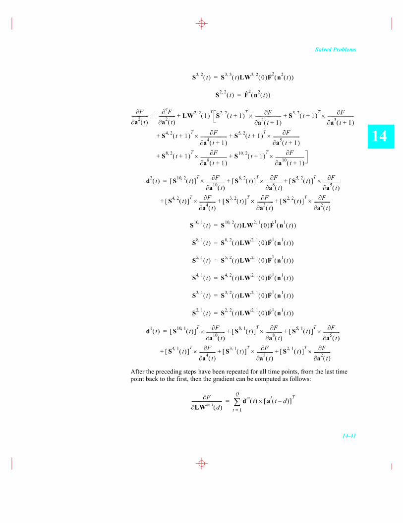
After the preceding steps have been repeated for all time points, from the last time point back to the first, then the gradient can be computed as follows:
S3 2, t( ) S3 3, t( )LW3 2, 0( )F· 2 n2 t( )( )=
S2 2, t( ) F· 2 n2 t( )( )=
Fa2 t( )
---------------eF
a2 t( )--------------- LW2 2, 1( )
TS2 2, t 1+( )
T Fa2 t 1+( )
------------------------× S3 2, t 1+( )T F
a3 t 1+( )------------------------×++=
S4 2, t 1+( )T F
a4 t 1+( )------------------------× S5 2, t 1+( )
T Fa5 t 1+( )
------------------------×+ +
S8 2, t 1+( )T F
a8 t 1+( )------------------------× S10 2, t 1+( )
T Fa10 t 1+( )
--------------------------×+ +
d2 t( ) S10 2, t( )[ ]T F
a10 t( )-----------------× S8 2, t( )[ ]
T Fa8 t( )
---------------× S5 2, t( )[ ]T F
a5 t( )---------------×+ +=
S4 2, t( )[ ]T F
a4 t( )---------------× S3 2, t( )[ ]
T Fa3 t( )
---------------× S2 2, t( )[ ]T F
a2 t( )---------------×+ + +
S10 1, t( ) S10 2, t( )LW2 1, 0( )F· 1 n1 t( )( )=
S8 1, t( ) S8 2, t( )LW2 1, 0( )F· 1 n1 t( )( )=
S5 1, t( ) S5 2, t( )LW2 1, 0( )F· 1 n1 t( )( )=
S4 1, t( ) S4 2, t( )LW2 1, 0( )F· 1 n1 t( )( )=
S3 1, t( ) S3 2, t( )LW2 1, 0( )F· 1 n1 t( )( )=
S2 1, t( ) S2 2, t( )LW2 1, 0( )F· 1 n1 t( )( )=
d1 t( ) S10 1, t( )[ ]T F
a10 t( )-----------------× S8 1, t( )[ ]
T Fa8 t( )
---------------× S5 1, t( )[ ]T F
a5 t( )---------------×+ +=
S4 1, t( )[ ]T F
a4 t( )---------------× S3 1, t( )[ ]
T Fa3 t( )
---------------× S2 1, t( )[ ]T F
a2 t( )---------------×+ + +
FLWm l, d( )
---------------------------- dm t( ) al t d�–( )[ ]T
×t 1=
Q
=
14 Dynamic Networks
14-42
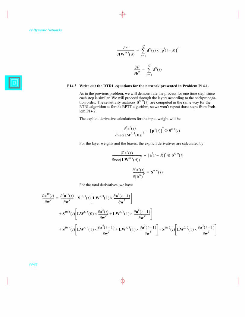
D P14.3 Write out the RTRL equations for the network presented in Problem P14.1.
As in the previous problem, we will demonstrate the process for one time step, since each step is similar. We will proceed through the layers according to the backpropaga-tion order. The sensitivity matrices are computed in the same way for the RTRL algorithm as for the BPTT algorithm, so we won�’t repeat those steps from Prob-lem P14.2.
The explicit derivative calculations for the input weight will be
For the layer weights and the biases, the explicit derivatives are calculated by
For the total derivatives, we have
FIWm l, d( )
-------------------------- dm t( ) pl t d�–( )[ ]T
×t 1=
Q
=
Fbm--------- dm t( )
t 1=
Q
=
Su m, t( )
eau t( )
vec IW1 1, 0( )( )T------------------------------------------ p1 t( )[ ]
TSu 1, t( )=
eau t( )
vec LWm l, d( )( )T-------------------------------------------- al t d�–( )[ ]
TSu m, t( )=
eau t( )
bm( )T----------------- Su m, t( )=
a10 t( )wT-----------------
ea10 t( )wT------------------- S10 9, t( ) LW9 8, 1( ) a8 t 1�–( )
wT------------------------×+=
S10 6, t( ) LW6 5, 0( ) a5 t( )wT---------------× LW6 5, 1( ) a5 t 1�–( )
wT------------------------×++
S10 4, t( ) LW4 4, 1( ) a4 t 1�–( )
wT------------------------× LW4 3, 1( ) a3 t 1�–( )
wT------------------------×+ S10 2, t( ) LW2 2, 1( ) a2 t 1�–( )
wT------------------------×+ +
Solved Problems
14-43
14
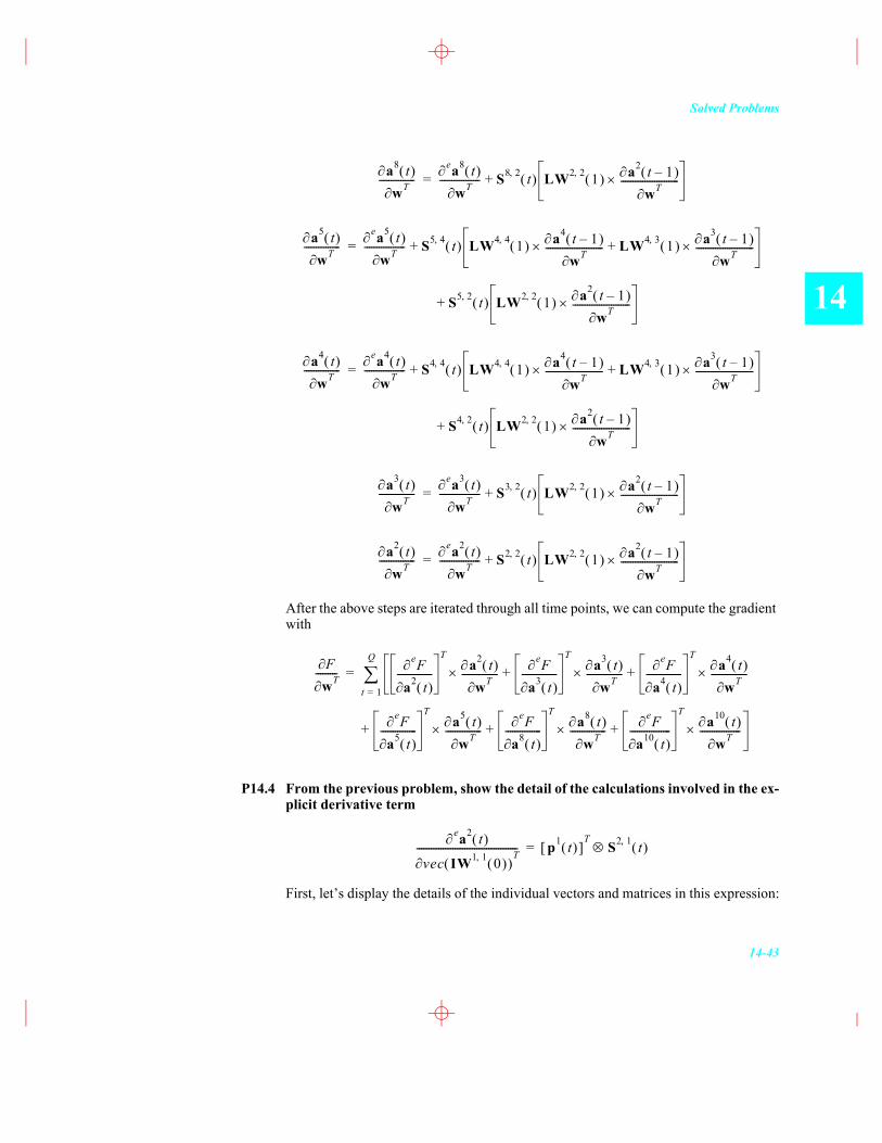
After the above steps are iterated through all time points, we can compute the gradient with
P14.4 From the previous problem, show the detail of the calculations involved in the ex-plicit derivative term
First, let�’s display the details of the individual vectors and matrices in this expression:
a8 t( )wT---------------
ea8 t( )wT----------------- S8 2, t( ) LW2 2, 1( ) a2 t 1�–( )
wT------------------------×+=
a5 t( )wT---------------
ea5 t( )wT----------------- S5 4, t( ) LW4 4, 1( ) a4 t 1�–( )
wT------------------------× LW4 3, 1( ) a3 t 1�–( )
wT------------------------×++=
S5 2, t( ) LW2 2, 1( ) a2 t 1�–( )
wT------------------------×+
a4 t( )wT---------------
ea4 t( )wT----------------- S4 4, t( ) LW4 4, 1( ) a4 t 1�–( )
wT------------------------× LW4 3, 1( ) a3 t 1�–( )
wT------------------------×++=
S4 2, t( ) LW2 2, 1( ) a2 t 1�–( )
wT------------------------×+
a3 t( )wT---------------
ea3 t( )wT----------------- S3 2, t( ) LW2 2, 1( ) a2 t 1�–( )
wT------------------------×+=
a2 t( )wT---------------
ea2 t( )wT----------------- S2 2, t( ) LW2 2, 1( ) a2 t 1�–( )
wT------------------------×+=
FwT---------
eFa2 t( )
---------------T
a2 t( )wT---------------×
eFa3 t( )
---------------T
a3 t( )wT---------------×
eFa4 t( )
---------------T
a4 t( )wT---------------×+ +
t 1=
Q
=
eFa5 t( )
---------------T
a5 t( )wT---------------×
eFa8 t( )
---------------T
a8 t( )wT---------------×
eFa10 t( )
-----------------T
a10 t( )wT-----------------×+ ++
ea2 t( )
vec IW1 1, 0( )( )T------------------------------------------ p1 t( )[ ]
TS2 1, t( )=
14 Dynamic Networks
14-44
D
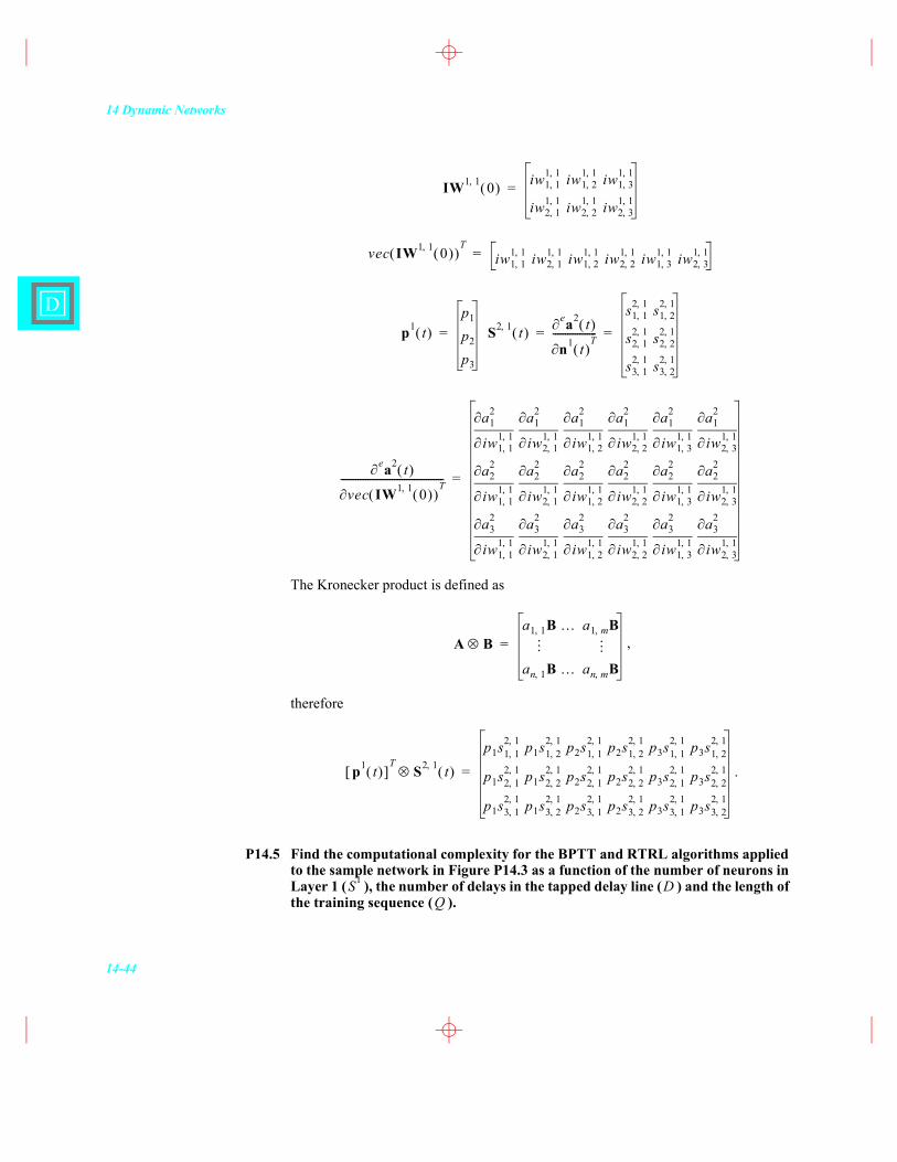
The Kronecker product is defined as
,
therefore
.
P14.5 Find the computational complexity for the BPTT and RTRL algorithms applied to the sample network in Figure P14.3 as a function of the number of neurons in Layer 1 ( ), the number of delays in the tapped delay line ( ) and the length of the training sequence ( ).
IW1 1, 0( ) iw1 1,1 1, iw1 2,
1 1, iw1 3,1 1,
iw2 1,1 1, iw2 2,
1 1, iw2 3,1 1,
=
vec IW1 1, 0( )( )T
iw1 1,1 1, iw2 1,
1 1, iw1 2,1 1, iw2 2,
1 1, iw1 3,1 1, iw2 3,
1 1,=
p1 t( )p1
p2
p3
= S2 1, t( )ea2 t( )
n1 t( )T------------------
s1 1,2 1, s1 2,
2 1,
s2 1,2 1, s2 2,
2 1,
s3 1,2 1, s3 2,
2 1,
= =
ea2 t( )
vec IW1 1, 0( )( )T------------------------------------------
iw1 1,1 1,
a12
iw2 1,1 1,
a12
iw1 2,1 1,
a12
iw2 2,1 1,
a12
iw1 3,1 1,
a12
iw2 3,1 1,
a12
iw1 1,1 1,
a22
iw2 1,1 1,
a22
iw1 2,1 1,
a22
iw2 2,1 1,
a22
iw1 3,1 1,
a22
iw2 3,1 1,
a22
iw1 1,1 1,
a32
iw2 1,1 1,
a32
iw1 2,1 1,
a32
iw2 2,1 1,
a32
iw1 3,1 1,
a32
iw2 3,1 1,
a32
=
A Ba1 1, B �… a1 m, B
an 1, B �… an m, B
= �… �…
p1 t( )[ ]T
S2 1, t( )
p1s1 1,2 1, p1s1 2,
2 1, p2s1 1,2 1, p2s1 2,
2 1, p3s1 1,2 1, p3s1 2,
2 1,
p1s2 1,2 1, p1s2 2,
2 1, p2s2 1,2 1, p2s2 2,
2 1, p3s2 1,2 1, p3s2 2,
2 1,
p1s3 1,2 1, p1s3 2,
2 1, p2s3 1,2 1, p2s3 2,
2 1, p3s3 1,2 1, p3s3 2,
2 1,
=
S1 DQ
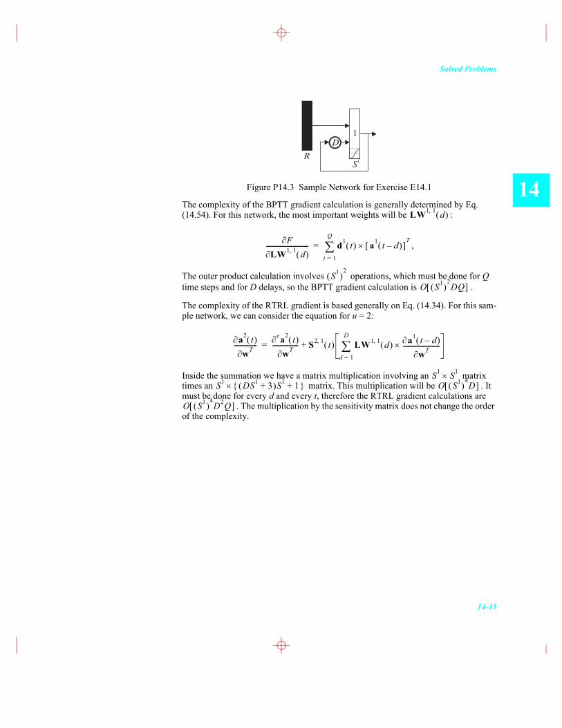
Solved Problems
14-45
14Figure P14.3 Sample Network for Exercise E14.1
The complexity of the BPTT gradient calculation is generally determined by Eq. (14.54). For this network, the most important weights will be :
,
The outer product calculation involves operations, which must be done for Q time steps and for D delays, so the BPTT gradient calculation is .
The complexity of the RTRL gradient is based generally on Eq. (14.34). For this sam-ple network, we can consider the equation for u = 2:
Inside the summation we have a matrix multiplication involving an matrix times an matrix. This multiplication will be . It must be done for every d and every t, therefore the RTRL gradient calculations are
. The multiplication by the sensitivity matrix does not change the order of the complexity.
DR
S1
1
LW1 1, d( )
FLW1 1, d( )
---------------------------- d1 t( ) a1 t d�–( )[ ]T
×t 1=
Q
=
S1( )2
O S1( )2DQ[ ]
a2 t( )wT---------------
ea2 t( )wT----------------- S2 1, t( ) LW1 1, d( ) a1 t d�–( )
wT------------------------×d 1=
D
+=
S1 S1×S1 DS1 3+( )S1 1+{ }× O S1( )
4D[ ]
O S1( )4D2Q[ ]

14 Dynamic Networks
14-46
D
EpilogueDynamic networks can be trained using the same optimization procedures which we described in Chapter 12 for static multilayer networks. However, the calculation of the gradient for dynamic networks is more complex than for static networks. There are two basic approaches to the gradient calculation in dynamic networks. One approach, backpropagation through time (BPTT), starts at the last time point, and works back-ward in time to compute the gradient. The second approach, real-time recurrent learn-ing (RTRL), starts at the first time point, and then works forward through time.
RTRL requires more calculations than BPTT for calculating the gradient, but RTRL allows a convenient framework for on-line implementation. Also, RTRL generally re-quires less storage than BPTT. For Jacobian calculations, RTRL is often more efficient than the BPTT algorithm.

Further Reading
14-47
14
Further Reading[DeHa07] De Jesús, O. and M. Hagan, �“Backpropagation Algorithms for a
Broad Class of Dynamic Networks,�” IEEE Transactions on Neural Networks, vol. 18, no. 1, pp., 2007.
This paper presents a general development of BPTT and RTRL al-gorithms for gradient and Jacobian calculations. Experimental re-sults are presented that compare the computational complexities of the two algorithms for a variety of network architectures.
[DeHo01] De Jesús, O., J. Horn, and M. Hagan, �“Analysis of Recurrent Net-work Training and Suggestions for Improvements,�” Proceedings of the International Joint Conference on Neural Networks, Washing-ton, DC, July 15-19, 2001, pp 2632-2637.
This paper describes spurious valleys that appear in the error surfac-es of recurrent networks. It also describes some procedures that can be used to improve training of recurrent networks.
[MaNe99] Magnus, J.R., and Neudecker, H., Matrix Differential Calculus, John Wiley & Sons, Ltd., Chichester, 1999.
This textbook provides a very clear and complete description of ma-trix theory and matrix differential calculus.
[Werb90] Werbos, P. J., �“Backpropagation through time: What it is and how to do it,�” Proceedings of the IEEE, vol. 78, pp. 1550�–1560, 1990.
The backpropagation through time algorithm is one of the two prin-cipal approaches to computing the gradients in recurrent neural net-work. This paper describes the general framework for backpropagation through time.
[WiZi89] Williams, R. J. and Zipser, D., �“A learning algorithm for continually running fully recurrent neural networks,�” Neural Computation, vol. 1, pp. 270�–280, 1989.
This paper introduced the real-time, recurrent learning algorithm for computing the gradients of dynamic networks. Using this method, the gradients are computed by starting at the first time point, and then working forward through time. The algorithm is suitable for on-line, or real-time, implementation.
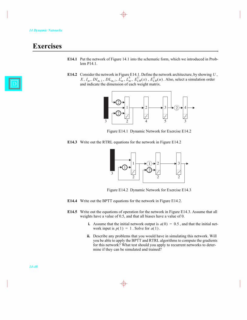
14 Dynamic Networks
14-48
D
ExercisesE14.1 Put the network of Figure 14.1 into the schematic form, which we introduced in Prob-
lem P14.1.
E14.2 Consider the network in Figure E14.1. Define the network architecture, by showing , , , , , , , , . Also, select a simulation order
and indicate the dimension of each weight matrix.
Figure E14.1 Dynamic Network for Exercise E14.2
E14.3 Write out the RTRL equations for the network in Figure E14.2
Figure E14.2 Dynamic Network for Exercise E14.3
E14.4 Write out the BPTT equations for the network in Figure E14.2.
E14.5 Write out the equations of operation for the network in Figure E14.3. Assume that all weights have a value of 0.5, and that all biases have a value of 0.
i. Assume that the initial network output is , and that the initial net-work input is . Solve for .
ii. Describe any problems that you would have in simulating this network. Will you be able to apply the BPTT and RTRL algorithms to compute the gradients for this network? What test should you apply to recurrent networks to deter-mine if they can be simulated and trained?
UX Im DIm 1, DLm l, Lm
f Lmb ELW
U x( ) ELWX u( )
22
2
3 4 5 32
2 3 41
121
32 22
21 3
a 0( ) 0.5=p 1( ) 1= a 1( )

Exercises
14-49
14Figure 14.12 Dynamic Network for Exercise E14.5
E14.6 One of the advantages of the RTRL algorithm is that the gradient can be computed at the same time as the network response, since it is computed by starting at the first time point, and then working forward through time. Therefore, RTRL allows a convenient framework for on-line implementation. Suppose that you are implementing the RTRL algorithm, and you update the weights of the network at each time step.
i. Discuss the accuracy of the gradient calculation if the weights are updated at each time step of a steepest descent algorithm.
ii. Implement the RTRL algorithm in MATLAB for the network in Figure 14.4. Generate training data by using the network with the two weights set equal to 0.5. Use the same input sequence shown in Figure 14.10, and use the network responses as the targets. Using this data set, train the network using the steepest descent algorithm, with a learning rate of . Set the initial weights to zero. Update the weights at each time step. Save the gradient at the end of the eighth time step.
iii. Repeat part ii., but do not update the weights. Compute the gradient at the end of the eighth time step. Compare this gradient with the one you obtained in part ii. Explain any differences
E14.7 Consider again the recurrent network of Figure 14.4. Assume that is the sum squared error for the first two time points.
i. Let . Find and as a functions of , , and the weights in the network.
ii. Find the sum squared error for the first two time steps as an explicit function of , , , , and the network weights.
iii. Using part (ii), find .
iv. Compare the results of part (iii) with the results determined by RTRL on page 14-21 and by BPTT on page 14-30.
E14.8 In the process of deriving the RTRL algorithm in Exercise E14.3, you should have pro-duced the following expression
11
1
1
» 2 + 2ans = 4
a t( )0.1=
F x( )
a 0( ) 0= a 1( ) a 2( ) p 1( ) p 2( )
p 1( ) p 2( ) t 1( ) t 2( )F
lw1 1, 1( )-----------------------
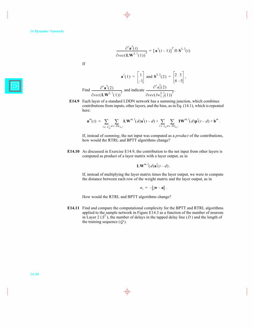
14 Dynamic Networks
14-50
D
If
and ,
Find and indicate .
E14.9 Each layer of a standard LDDN network has a summing junction, which combines contributions from inputs, other layers, and the bias, as in Eq. (14.1), which is repeated here:
.
If, instead of summing, the net input was computed as a product of the contributions, how would the RTRL and BPTT algorithms change?
E14.10 As discussed in Exercise E14.9, the contribution to the net input from other layers is computed as product of a layer matrix with a layer output, as in
.
If, instead of multiplying the layer matrix times the layer output, we were to compute the distance between each row of the weight matrix and the layer output, as in
.
How would the RTRL and BPTT algorithms change?
E14.11 Find and compare the computational complexity for the BPTT and RTRL algorithms applied to the sample network in Figure E14.3 as a function of the number of neurons in Layer 2 ( ), the number of delays in the tapped delay line ( ) and the length of the training sequence ( ).
ea3 t( )
vec LW2 1, 1( )( )T-------------------------------------------- a1 t 1�–( )[ ]
TS3 2, t( )=
a1 1( ) 11�–
= S3 2, 2( ) 2 34 5�–
=
ea3 2( )
vec LW2 1, 1( )( )T--------------------------------------------
ea13 2( )
vec lw1 2,2 1, 1( )( )
T----------------------------------------
nm t( ) LWm l, d( )al t d�–( )d DLm l,l Lm
f
IWm l, d( )pl t d�–( )d DIm l,l Im
bm+ +=
LWm l, d( )al t d�–( )
ni wi a�–�–=
S2 DQ
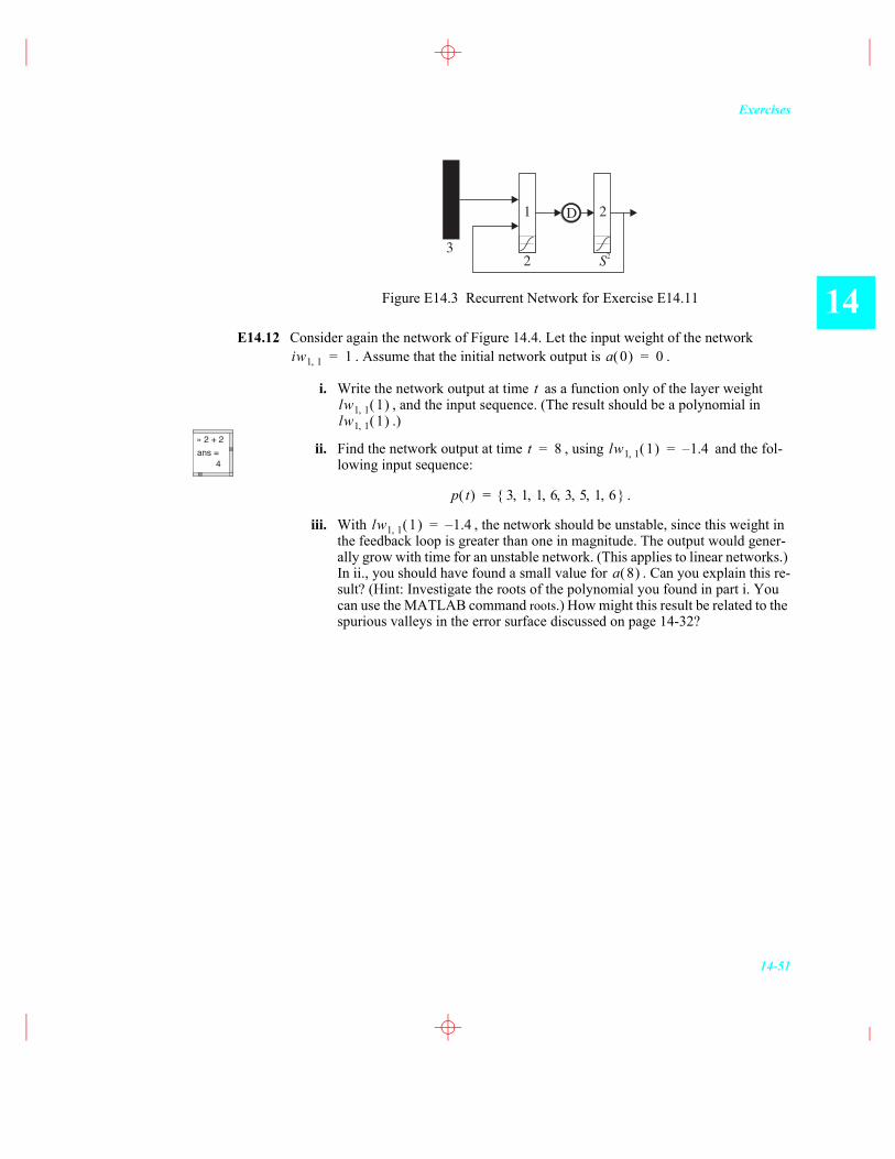
Exercises
14-51
14Figure E14.3 Recurrent Network for Exercise E14.11
E14.12 Consider again the network of Figure 14.4. Let the input weight of the network . Assume that the initial network output is .
i. Write the network output at time as a function only of the layer weight , and the input sequence. (The result should be a polynomial in .)
ii. Find the network output at time , using and the fol-lowing input sequence:
.
iii. With , the network should be unstable, since this weight in the feedback loop is greater than one in magnitude. The output would gener-ally grow with time for an unstable network. (This applies to linear networks.) In ii., you should have found a small value for . Can you explain this re-sult? (Hint: Investigate the roots of the polynomial you found in part i. You can use the MATLAB command roots.) How might this result be related to the spurious valleys in the error surface discussed on page 14-32?
D
32 S2
1 2
iw1 1, 1= a 0( ) 0=
tlw1 1, 1( )lw1 1, 1( )
» 2 + 2ans = 4
t 8= lw1 1, 1( ) 1.4�–=
p t( ) 3 1 1 6 3 5 1 6, , , , , , ,{ }=
lw1 1, 1( ) 1.4�–=
a 8( )

14 Dynamic Networks
14-52
D
Related Documents