Numerical Solution of Ill-posed Cauchy Problems …liu.diva-portal.org › smash › get › diva2:302609 › FULLTEXT01.pdfAbstract Ranjbar, Z. (2010). Numerical Solution of Ill-posed

Linköping Studies in Science and Technology. Dissertations.No. 1300

Numerical Solution of Ill-posedCauchy Problems for Parabolic

Equations

Zohreh Ranjbar

Department of MathematicsScientific Computing

Linköping 2010

Cover page courtesy of Dennis Netzell

Linköping Studies in Science and Technology. Dissertations.No. 1300

Numerical Solution of Ill-posed Cauchy Problems for Parabolic Equations

Zohreh Ranjbar

[email protected]

Department of MathematicsScientific ComputingLinköping UniversitySE–581 83 Linköping

Sweden

ISBN 978-91-7393-443-5 ISSN 0345-7524

Copyright c© 2010 Zohreh Ranjbar

Printed by LiU-Tryck, Linköping, Sweden 2010

To Atra, Mohsen and my parents

Abstract

Ranjbar, Z. (2010). Numerical Solution of Ill-posed Cauchy Problems forParabolic Equations. Doctoral dissertation.ISBN 978-91-7393-443-5. ISSN 0345-7524.

Ill-posed mathematical problem occur in many interesting scientific and engineering ap-plications. The solution of such a problem, if it exists, may not depend continuously on theobserved data. For computing a stable approximate solution it is necessary to apply a reg-ularization method. The purpose of this thesis is to investigate regularization approachesand develop numerical methods for solving certain ill-posed problems for parabolic par-tial differential equations. In thermal engineering applications one wants to determine thesurface temperature of a body when the surface itself is inaccessible to measurements.This problem can be modelled by a sideways heat equation. The mathematical and nu-merical properties of the sideways heat equation with constant convection and diffusioncoefficients is first studied. The problem is reformulated as a Volterra integral equationof the first kind with smooth kernel. The influence of the coefficients on the degree ofill-posedness are also studied. The rate of decay of the singular values of the Volterraintegral operator determines the degree of ill-posedness. It is shown that the sign of thecoefficient in the convection term influences the rate of decay of the singular values.

Further a sideways heat equation in cylindrical geometry is studied. The equation is amathematical model of the temperature changes inside a thermocouple, which is used toapproximate the gas temperature in a combustion chamber. The heat transfer coefficientat the surface of thermocouple is also unknown. This coefficient is approximated via acalibration experiment. Then the gas temperature in the combustion chamber is computedusing the convection boundary condition. In both steps the surface temperature and heatflux are approximated using Tikhonov regularization and the method of lines.

Many existing methods for solving sideways parabolic equations are inadequate forsolving multi-dimensional problems with variable coefficients. A new iterative regular-ization technique for solving a two-dimensional sideways parabolic equation with vari-able coefficients is proposed. A preconditioned Generalized Minimum Residuals Method(GMRS) is used to regularize the problem. The preconditioner is based on a semi-analyticsolution formula for the corresponding problem with constant coefficients. Regularizationis used in the preconditioner as well as truncating the GMRES algorithm. The computedexamples indicate that the proposed PGMRES method is well suited for this problem.

In this thesis also a numerical method is presented for the solution of a Cauchy prob-lem for a parabolic equation in multi-dimensional space, where the domain is cylindricalin one spatial direction. The formal solution is written as a hyperbolic cosine functionin terms of a parabolic unbounded operator. The ill-posedness is dealt with by truncatingthe large eigenvalues of the operator. The approximate solution is computed by projectingonto a smaller subspace generated by the Arnoldi algorithm applied on the inverse of theoperator. A well-posed parabolic problem is solved in each iteration step. Further thehyperbolic cosine is evaluated explicitly only for a small triangular matrix. Numericalexamples are given to illustrate the performance of the method.

v

Populärvetenskaplig sammanfattning

Inom många vetenskapliga och tekniska tillämpningar är det nödvändigt att uppskattavissa parametrar som kännetecknar ett fysiskt system, men som är oåtkomliga för direktamätningar. Detta problemområde, så kallade inversa problem, har blivit ett mycket aktivtoch väletablerat tvärvetenskapligt forskningsområde under de senaste tre decennierna.Det täcker bl a problem från teknik, industri, medicin, liksom livs- och geovetenskaper.

Ett exempel på ett inverst problem inom värmeteknik är att man vill bestämma yttem-peraturen hos ett objekt när ytan i sig är oåtkomlig för mätning. Det kan också vara så attlokalisering av en mätenhet på ytan skulle störa mätningarna så att en felaktig tempera-tur registreras. I sådana fall är man begränsad till interna mätningar. Detta problem kanmodelleras med en värmeledningsekvation, som löses i sidled, dvs i rumsled, till skillnadfrån standardproblemet som löses framåt i tiden. Inversa problem är ofta illa-ställda. Lös-ningen till ett illa-ställt matematiskt problem, om den existerar, beror inte kontinuerligtpå observerade data. Detta innebär t.ex. att små fel i uppmätta temperaturer kan leda tillmycket stora fel i den beräknade lösningen. I praktiken uppstår fel i uppmätta data ochdet är därför nödvändigt att tillämpa en regulariseringsmetod, som gör lösningen mindrekänslig för störningar i uppmätta data.

Syftet med denna avhandling är att undersöka regulariseringsstrategier och utvecklanumeriska metoder för att lösa vissa illa-ställda problem för paraboliska partiella differen-tial ekvationer. Vi studerar först påverkan av koefficienterna i värmeledningsekvationen isidled på graden av illa-ställdhet. Vi löser också en värmeledningsekvation i sidled, därekvationen är en matematisk modell av temperaturförändringar inuti ett termoelement,som används för att approximera gastemperaturen i en förbränningskammare.

Många metoder för att lösa paraboliska ekvationer i sidled är otillräckliga för att lösamulti-dimensionella problem med variabla koefficienter. En ny iterativ regulariserings-teknik för att lösa en två-dimensionell parabolisk ekvation i sidled med variabla koeffi-cienter föreslås. I en iterativ metod startar man med en begynnelseapproximation, somsedan gradvis förbättras. Eftersom iterationerna för denna typ av problem först förbätt-rar approximationen men senare försämrar den, kan man regularisera genom att stoppaiterationer vid lämplig tidpunkt.

I denna avhandling presenteras också en numerisk metod för lösning av ett paraboliskinverst problem i ett flerdimensionellt rum, där området är cylindriskt i en rumsriktning.Den approximativa lösningen beräknas genom att projicera på ett underrum genererat aven Krylovsrumsmetod.

vii

Acknowledgments

Through out the long and occasionally rocky process of this thesis I have been supportedby many people. It is a pleasure to convey my thanks to all of them who made this workpossible.

I wish to express my sincerest gratitude to my supervisor Prof. Lars Eldén for hisencouraging and stubborn guidance during this work. I am also very grateful for his mostmeticulous and thorough revision, professional insights and tireless generosity.

I would like to thank Dr. Fredrik Berntsson whose expertise and interesting discus-sions helped very much along the work. I am grateful to Prof. Dan Loyd and ElisabethBlom at the Department of Management and Engineering, Linköping University, for help-ful discussions about heat transfer problems. I am also indebted to present and formercolleagues at the Department of Mathematics, particularly at the Division of ScientificComputing, for providing a good working environment and sharing experiences with me.I am grateful to Dr. Martin Ohlsson for letting me use the LaTeX layout of his thesis. Ireally thank the administrative staff for all their support in administering my fellowship.

I would also like to take the chance and thanks my family, my husband Mohsen for hisvaluable support and continuous encouragement and my parents for their unconditionallove and dedication and the many years of support during my undergraduate studies thatprovided the foundation for this work. I deeply thank my sister Zahra and her family whosupported me from the first day I came to Sweden. Thanks also to my other siblings inIran for their love and for believing in me. I am also very grateful to my friends, myparents-in-law and other relatives who helped me during these challenging years.

Linköping, February 25, 2010

Zohreh Ranjbar

ix

Contents

1 Introduction and Overview 11 Inverse Ill-Posed Problems and Ill-Conditioning . . . . . . . . . . . . . . 12 Cauchy Problems for Parabolic Equations . . . . . . . . . . . . . . . . . 2

2.1 Sideways Heat Equations . . . . . . . . . . . . . . . . . . . . . . 22.2 Ill-Posedness and Singular Values . . . . . . . . . . . . . . . . . 4

3 Direct Regularization Methods . . . . . . . . . . . . . . . . . . . . . . . 53.1 Truncated Singular Value Decomposition . . . . . . . . . . . . . 53.2 Tikhonov Regularization . . . . . . . . . . . . . . . . . . . . . . 63.3 Method of Lines . . . . . . . . . . . . . . . . . . . . . . . . . . 6

4 Iterative Regularization Methods . . . . . . . . . . . . . . . . . . . . . . 64.1 Classical Stationary Methods . . . . . . . . . . . . . . . . . . . . 74.2 Krylov Subspace Methods . . . . . . . . . . . . . . . . . . . . . 7

5 Choice of Regularization Parameter . . . . . . . . . . . . . . . . . . . . 8

2 Summary of Papers 9

Bibliography 11

Appended Manuscripts 17

I Numerical Analysis of an Ill-Posed Cauchy Problem for a Convection-DiffusionEquation 191 Introduction . . . . . . . . . . . . . . . . . . . . . . . . . . . . . . . . . 222 Derivation of a Volterra Integral Equation . . . . . . . . . . . . . . . . . 23

2.1 The Kernel Function for Different Values ofa andb . . . . . . . 283 Singular Value Analysis of the Volterra Equation . . . . . . . . . . . . . 28

xi

Contents

4 Eigenvalue Analysis of the Cauchy Problem . . . . . . . . . . . . . . .. 325 Numerical Experiments . . . . . . . . . . . . . . . . . . . . . . . . . . . 356 Concluding Remarks . . . . . . . . . . . . . . . . . . . . . . . . . . . . 36A Appendix . . . . . . . . . . . . . . . . . . . . . . . . . . . . . . . . . . 38B Appendix . . . . . . . . . . . . . . . . . . . . . . . . . . . . . . . . . . 39References . . . . . . . . . . . . . . . . . . . . . . . . . . . . . . . . . . . . . 40

II A Sideways Heat Equation Applied to the Measurement of the Gas Temper-ature in a Combustion Chamber 431 Introduction . . . . . . . . . . . . . . . . . . . . . . . . . . . . . . . . . 462 Mathematical Modelling and Computational Procedures . . . . . . . . . 483 Computation of the Gas Temperature . . . . . . . . . . . . . . . . . . . . 50

3.1 Approximating the Surface Temperature and Heat Flux . . . . . . 503.2 Solving the Inverse Problem in the Region of Magnesium Oxide . 513.3 Solving the Inverse Problem in the Steel Domain . . . . . . . . . 533.4 Approximating the Gas Temperature . . . . . . . . . . . . . . . . 54

4 Calibration . . . . . . . . . . . . . . . . . . . . . . . . . . . . . . . . . 544.1 Approximating the Surface Temperature and Heat Flux . . . . . 544.2 Computingh . . . . . . . . . . . . . . . . . . . . . . . . . . . . 56

5 Numerical Experiments . . . . . . . . . . . . . . . . . . . . . . . . . . . 566 Concluding remarks . . . . . . . . . . . . . . . . . . . . . . . . . . . . . 637 Acknowledgment . . . . . . . . . . . . . . . . . . . . . . . . . . . . . . 66A Appendix . . . . . . . . . . . . . . . . . . . . . . . . . . . . . . . . . . 66References . . . . . . . . . . . . . . . . . . . . . . . . . . . . . . . . . . . . . 68

III A Preconditioned GMRES Method for Solving a Sideways Parabolic Equa-tion in Two Space Dimensions 711 Introduction . . . . . . . . . . . . . . . . . . . . . . . . . . . . . . . . . 742 Preconditioned GMRES . . . . . . . . . . . . . . . . . . . . . . . . . . 763 The One-Dimensional Sideways Heat Equation . . . . . . . . . . . . . . 77

3.1 Circulant Preconditioning . . . . . . . . . . . . . . . . . . . . . 783.2 1D Numerical Experiments . . . . . . . . . . . . . . . . . . . . . 81

4 The Two-Dimensional Sideways Parabolic Equation . . . . . . . . . . . . 874.1 Constant Coefficients: Analysis . . . . . . . . . . . . . . . . . . 874.2 Preconditioned GMRES for the 2D Problem . . . . . . . . . . . . 934.3 Preconditioner . . . . . . . . . . . . . . . . . . . . . . . . . . . 944.4 Numerical Experiments . . . . . . . . . . . . . . . . . . . . . . 95

5 Conclusions . . . . . . . . . . . . . . . . . . . . . . . . . . . . . . . . . 101A Appendix . . . . . . . . . . . . . . . . . . . . . . . . . . . . . . . . . . 103B Appendix . . . . . . . . . . . . . . . . . . . . . . . . . . . . . . . . . . 104References . . . . . . . . . . . . . . . . . . . . . . . . . . . . . . . . . . . . . 105

IV Numerical Solution of a Cauchy Problem for a Parabolic Equation in Twoor more Space Dimensions by the Arnoldi Method 1091 Introduction . . . . . . . . . . . . . . . . . . . . . . . . . . . . . . . . . 1122 Ill-posedness and Regularization . . . . . . . . . . . . . . . . . . . . . . 113

xii

2.1 Regularization Based on Fourier Transform and Eigenvalue Ex-pansion . . . . . . . . . . . . . . . . . . . . . . . . . . . . . . . 113

3 Arnoldi Recursion and Decomposition . . . . . . . . . . . . . . . . . . 1153.1 Implementation . . . . . . . . . . . . . . . . . . . . . . . . . . . 117

4 Arnoldi-Truncated Schur Factorization . . . . . . . . . . . . . . . . . . . 1174.1 Accuracy of Truncated Approximation . . . . . . . . . . . . . . 118

5 Arnoldi-TSVD Method . . . . . . . . . . . . . . . . . . . . . . . . . . . 1206 Numerical Examples . . . . . . . . . . . . . . . . . . . . . . . . . . . . 1207 Summary and Future Work . . . . . . . . . . . . . . . . . . . . . . . . . 121A Appendix . . . . . . . . . . . . . . . . . . . . . . . . . . . . . . . . . . 129

A.1 Proof of Lemma 2.1 . . . . . . . . . . . . . . . . . . . . . . . . 129A.2 Proof of Theorem 2.1 . . . . . . . . . . . . . . . . . . . . . . . . 130

References . . . . . . . . . . . . . . . . . . . . . . . . . . . . . . . . . . . . . 131

xiii

1Introduction and

Overview

IN many scientific and engineering applications there is a need to estimate some pa-rameters characterizing a physical system, which is inaccessible to direct measure-

ments.This problem area, so calledinverse problems, has become a very active, interdisci-plinary and well-established research area over the past three decades. It covers problemsfrom engineering, industry, medicine, as well as life and earth sciences. Some examplesof inverse problems are computerized tomography [50], inverse scattering problems [24],inverse problems in geophysics [25]. One particular area of inverse problems is inheatconduction[1], where the goal is to reconstruct the values of the parameters character-izing the system from a noisy measured temperature. A classic problem of inverse heatconduction is thebackward problem, where the initial conditions (temperature) are tobe found from later measurements. Numerical solutions of this problem have been con-sidered in [17, 61, 60, 40, 42]. Another interesting problem is Sideways Heat Equation(SHE) problem, where the unknown temperature at the boundary of the object is to beapproximated based on measurements of the accessible temperature of the object. Theheat equationis a prototype parabolic partial differential equation (PDE), used to modelheat conduction in a given region over time. The aim of this thesis is to investigate thenumerical solution of certain sideways parabolic PDE problems.

1 Inverse Ill-Posed Problems and Ill-Conditioning

Inverse problems are oftenill-posed, as opposed to the well-posed problems introducedby Hadamard [31]. Consider the linear operator equation

Kf = g, (1.1)

whereK : H1 → H2 is a bounded linear operator between Hilbert spacesH1 andH2.

Definition 1.1. The problem of solving (1.1) is calledwell-posedif:

1

1 Introduction and Overview

1. Existence: a solution exists for any datag in the data space.

2. Uniqueness: the solutionf is unique in the solution space.

3. Stability: the solutionf depends continuously on the datag.

Conditions 1 and 2 are equivalent to saying that the operatorK has a well definedinverseK−1 and that the range ofK is all of the data space. The condition 3 is equivalentto K−1 being continuous or bounded. For inverse problems this stability condition ismost often violated. To stabilize the solution, one needs to incorporate additional a prioriinformation into the problem, so calledregularization.

In many linear ill-posed problems that arise in science and engineering, instead of theexact right hand sideg, only a perturbation of it,gδ = g + δ, is available. When theinverse operatorK−1 is unbounded, it means that if the solutionf exists then the solutionfδ = K−1gδ is usually a poor approximation off , even for very small values ofδ.

While inverse problems are often formulated in infinite dimensional spaces, limita-tions to a finite number of measurements, and the practical consideration of recoveringonly a finite number of unknown parameters leads to stating the problem in discrete form.Following [35], a problem is calleddiscrete ill-posedwhen it is highly sensitive to high-frequency perturbations and the solution operator has very large norm.

2 Cauchy Problems for Parabolic Equations

A parabolic Cauchy problem (initial-boundary value problem) is a PDE that satisfies cer-tain conditions which are given on the boundary of the domain. As a simple example of aone-dimensional ill-posed Cauchy problem for the heat equation we have,

ut = uxx, 0 < x < 1, 0 ≤ t ≤ 1,u(x, 0) = 0, 0 ≤ x ≤ 1,u(0, t) = g(t), 0 ≤ t ≤ 1,ux(0, t) = h(t), 0 ≤ t ≤ 1.

(1.2)

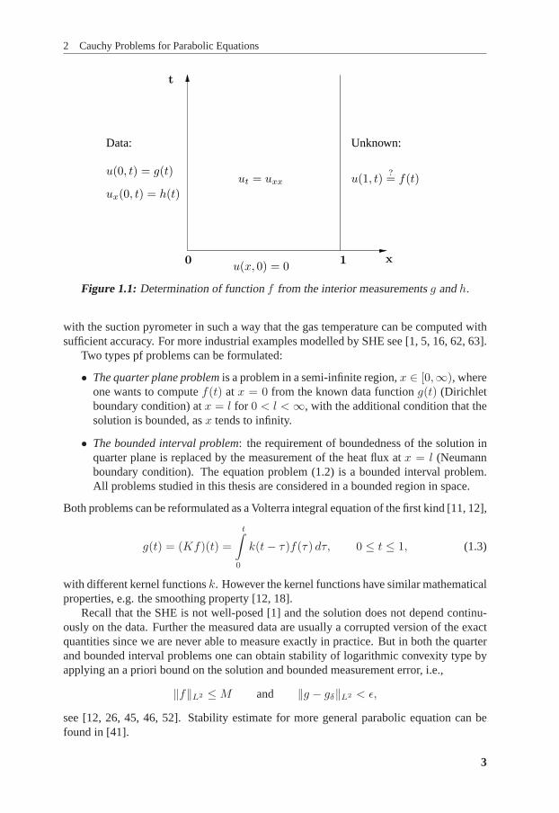
From the data at the left boundary we want to determine the solution at the right boundaryu(1, t) = f(t), see Figure 1.1. This is a sideways heat equation in a bounded domain.From now on we consider all the involved functions to be inL2.

2.1 Sideways Heat Equations

The sideways heat equation (SHE) (1.2) is an ill-posed Cauchy problem for a parabolicequation. It is sometimes referred as the inverse heat conduction problem [1, 49]. Welabel it the SHE in order to distinguish it from other inverse problems for a parabolicequation [12]. In this definition the initial temperature distribution is considered known.The linearity of the differential equation implies that initial data can easily be taken equalto zero. In Paper II we consider a SHE as a simple model of the heat transfer inside athermocouple of a suction pyrometer. The suction pyrometer [8], is used for measuringand controlling the gas temperature in a combustion chamber. The numerical experimentsin this paper, with synthetic data, indicate that it is possible to organize the measurements

2

2 Cauchy Problems for Parabolic Equations

Data:

u(0, t) = g(t)

t

10

ux(0, t) = h(t)

u(x, 0) = 0

u(1, t)?= f(t)

Unknown:

x

ut = uxx

Figure 1.1: Determination of functionf from the interior measurementsg andh.

with the suction pyrometer in such a way that the gas temperature can be computed withsufficient accuracy. For more industrial examples modelled by SHE see [1, 5, 16, 62, 63].

Two types pf problems can be formulated:

• The quarter plane problemis a problem in a semi-infinite region,x ∈ [0,∞), whereone wants to computef(t) at x = 0 from the known data functiong(t) (Dirichletboundary condition) atx = l for 0 < l <∞, with the additional condition that thesolution is bounded, asx tends to infinity.

• The bounded interval problem: the requirement of boundedness of the solution inquarter plane is replaced by the measurement of the heat flux atx = l (Neumannboundary condition). The equation problem (1.2) is a bounded interval problem.All problems studied in this thesis are considered in a bounded region in space.

Both problems can be reformulated as a Volterra integral equation of the first kind [11, 12],

g(t) = (Kf)(t) =

t∫

0

k(t− τ)f(τ) dτ, 0 ≤ t ≤ 1, (1.3)

with different kernel functionsk. However the kernel functions have similar mathematicalproperties, e.g. the smoothing property [12, 18].

Recall that the SHE is not well-posed [1] and the solution does not depend continu-ously on the data. Further the measured data are usually a corrupted version of the exactquantities since we are never able to measure exactly in practice. But in both the quarterand bounded interval problems one can obtain stability of logarithmic convexity type byapplying an a priori bound on the solution and bounded measurement error, i.e.,

‖f‖L2 ≤M and ‖g − gδ‖L2 < ǫ,

see [12, 26, 45, 46, 52]. Stability estimate for more general parabolic equation can befound in [41].

3

1 Introduction and Overview

In the Volterra integral equation (1.3) we have acausality principle[19] in the sensethat what happens at the “solution” boundary at timet0 can only affect the datag(t) fort ≥ t0. Therefore the solutionf(t) can not be reconstructed fort close to the final time1.This is another reason of ill-posedness of the SHE beside the smoothness of the Volterraoperator. Note that the coefficients of SHE play a role for the smoothness of the Volterraoperator (ill-posedness) which is analyzed and illustrated in Paper I.

A common family of methods for solving the SHE transforms the problem into anintegral equation of first kind. The weak point of these methods is that often the kernelin the corresponding integral equation is not known explicitly, e.g., when the differentialequations has variable coefficients.

2.2 Ill-Posedness and Singular Values

Singular values and singular functions of the operator give information about the natureof ill-posedness, for more details see [24, chapter 2]. If in (1.3) the kernel functionk ∈L2([0, 1] × [0, 1]) then the operatorK is compact and the inverse operatorK−1 existsand is unbounded [12]. For any compact operator we have the following definition of asingular system.

Definition 2.1. The set(σn, un, vn)∞n=1 is thesingular systemof the compact operatorK : H1 → H2, if

Kvn = σnun, K∗un = σnvn,

where the singular values are ordered,σ1 ≥ σ2 ≥ · · · > 0, and the sets of singularfunctions{un}∞n=1 and{vn}∞n=1 constitute complete orthonormal systems.

The operatorK∗ : H2 → H1 is the adjoint ofK. For compact operators the sin-gular values have only one accumulation point0, which meanslimn→∞ σn = 0. Thediscrete analogue of the above singular system is a singular value decomposition (SVD)of a rectangular matrix [28, p.70], and is considered later in this chapter. The singularvalue expansion (SVE) of the operator is

Kf =

∞∑

n=1

σn(f, vn)un, K∗g =

∞∑

n=1

σn(g, un)vn.

Formally the solution ofKf = g can be written

f = K†g =

∞∑

n=1

(g, un)

σnvn, (1.4)

The operatorK† is called theMoore-Penrose pseudo-inverse[24]. The following condi-tion for the existence of a solution is called thePicard criterion,

‖f‖2L2 =

∞∑

n=1

|(g, un)|2σ2n

<∞. (1.5)

This implies that(g, un) must decay more rapidly asn → ∞ thanσn, which means thatthe data functiong that satisfies the Picard condition must be very smooth. In practice, due

4

3 Direct Regularization Methods

to the measurement error we have inexact datagδ = g+ δ. Since the measurement errorsare usually stochastic we can not assume that the functionδ satisfies the Picard condition.Therefore in the case of measurement errors (even very small) any naive solution viathe infinite sum (1.4) usually diverges or has a very large norm. The analogue of thecondition (1.5), which should be satisfied by the solution of a finite dimensional linearsystem is called thediscrete Picard condition, introduced in [34].

The Volterra operator (1.3) in discrete form is a triangular Toeplitz matrix which isextremely ill-conditioned. Even for noise free measured datag, applying the least squaressolution of solving this ill-conditioned system always exhibits very large oscillations dueto round-off error in the computer arithmetic.

Therefore there is a need to regularize the problem. There are various approachesto regularizing and stabilizing the ill-posedness of parabolic Cauchy problems, see e.g.,[24, 40, 3] and the references therein. In the following we will give a short presentationof some regularization methods for discrete ill-posed problems.

3 Direct Regularization Methods

Direct regularization method can be based on some decomposition in numerical linearalgebra like, e.g. Singular Value Decomposition (SVD) or orthogonal transformation.These methods require a direct access to all elements of matrixK when solving the linearsystemKf = g. Some methods based onFourier transform where the ill-posednessis dealt with by cutting off the high frequencies are proposed in [2, 22, 53, 59]. In thisthesis the following direct methods are employed: Tikhonov regularization in discreteform (Papers I-III), truncated SVD (Papers III, IV), a method of lines combined with theapproximation of the time derivative by a bounded operator (Paper I-III). These methodswill be discussed shortly in following subsections.

Other examples of regularization methods for solving ill-posed Cauchy parabolicproblems are the method ofBeck[1], mollification[48] andvariational methods[44, 38].

3.1 Truncated Singular Value Decomposition

The association of small singular values with ill-posedness has been discussed in the pre-vious section. Therefore an obvious idea to regularize the problem is to truncate the smallsingular values of the operator i.e. truncate the series (1.4). Suppose that the operatorKin (1.1) is discretized to an× n matrix with the following singular value decomposition

K =n∑

i=1

σiuivTi ,

whereσ1 > σ2 > · · · > σn ≥ 0 are the singular values anduk andvk are the left andright singular vectors, respectively. The solution toKf = gδ can be written

f =n∑

i=1

uTi gδσi

vi.

Recall that small perturbations in the coefficientsuTi gδ are magnified extremely by afactorσ−1

i for i large enough, because the most of singular values{σi} are very small.

5

1 Introduction and Overview

The truncated singular value decomposition (TSVD) method only utilizes theN ≤ nlargest singular values for the solution and damps the effects caused by division by thesmall singular values, i.e. the TSVD solution is

fN =N∑

i=1

uTi gδσi

vi.

The number of termsN is the regularization parameter which should be properly selectedto get a good accuracy of the approximated solution.

3.2 Tikhonov Regularization

Tikhonov regularization is one of the most commonly used methods for regularization ofill-posed problems. The goal is to minimize‖g−Kf‖2 subject to a constraint on the sizeor smoothness of thef . The regularized solution solves the problem,

minf

‖g −Kf‖2 + λ‖Lf‖2,

whereλ > 0 is the regularization parameter and the matrixL is either the identity matrixor a discrete differentiation operator. The parameterλ controls the smoothness of thesolution. In other words it is a trade-off between fitting the data and reducing a normof the solution. Both Tikhonov and TSVD are expensive to implement for large-scaleapplications. For more details about these two methods we refer to [24, 35].

3.3 Method of Lines

The idea of the method of lines is to rewrite the original PDE (1.2) as a system of Ordi-nary Differential Equation (ODE). The source of ill-posedness is that the time derivative∂u/∂t is unbounded, see [19, 21, 55]. Therefore by replacing the time derivative by abounded approximation one can regularize the problem. Afterwards the resulting initial-value problem can be solved numerically essentially as an ODE in the space variable. Thisis a reason to treat the space and time discretization separately. There are some methods toapproximate the time derivative, like difference quotient [20], wavelet-Galerkin [55, 56],mollification approximation [39, 48], spectral in terms of Fast Fourier Transform(FFT)[2], spline approximation [4]. We have used the last two methods in Papers I and II.

4 Iterative Regularization Methods

Iterative regularization methods are based on iteration schemes that access the matrixKonly via matrix-vector multiplications. This property is suitable for sparse matrices andalso when solving problems, where the matrix is not explicitly available. Many iterativemethods have a self regularizing property in that early termination of the iterative processhas a regularizing effect. The approximate solution initially tends to the true solution andthen it diverges to some other undesired vector in later stages of iteration. This is calledthesemi-convergencephenomenon of iterative methods applied to ill-posed problems [24,

6

4 Iterative Regularization Methods

chapter 6]. In other words, the iteration number can be considered as a regularization pa-rameter. This is due to the fact that in its first few steps the iterative method approximatesmainly solution components associated with the largest singular values. Then graduallythe smaller singular values start to influence the solution and finally after many steps,those singular values that are close to zero are approximated, which makes the solutionexplode. Therefore iterative methods may give useful results if terminated early.

4.1 Classical Stationary Methods

One of the first iterative regularization methods is the Landweber iteration, which is avariant of the steepest-descent method for least square problems, see [24, chapter 6].Such methods are known as stationary methods. The Landweber iteration method hasvery slow convergence compared to Krylov subspace methods. The Landweber methodis most used in signal and image processing, see e.g., [6, 54] and references therein. Theiterative method proposed in [15] also can be viewed as a Landweber type method.

4.2 Krylov Subspace Methods

Some of the best known Krylov subspace methods are the conjugate gradient (CG),Arnoldi and generalized minimum residual (GMRES) methods, see [58]. The CG al-gorithm is used for solving sparse symmetric positive definite (SPD) linear systems [30].In [42, 57] a CG type method based on minimizing a certain functional is proposed tosolve a backward heat conduction problem. For a description about the regularizationproperty of CG we refer to [24, chapter 7].

The Arnoldi method is used to solve both large and sparse linear systems and eigen-value problems by projecting the problem onto a Krylov subspace of smaller dimensionm < n. GivenK ∈ R

n×n andg ∈ Rn theKrylov subspaceof dimensionm is defined by

Km(K, g) = span{g,Kg,K2g, . . . ,Km−1g}.

Let v1 = g/‖g‖ then the orthonormal basisVm = [v1, . . . , vm] of Krylov subspaceKm(K, g) can be obtained one vector at a time by computingKvj and orthonormalizingthis vector against all previousvi’s by modified Gram-Schmidt procedure. This gives arelation of the form

KVm = VmHm + hm+1,mvm+1eTm, (1.6)

whereHm is am×m Hessenberg matrix containing the orthonormalization coefficients.Further by regularizing the Hessenberg matrix we can find a good approximation of theoriginal problem recovered from the solution of projected problem [7, 23, 27, 51].

The GMRES method is based on the Arnoldi recursion and can be used for solvinglinear systems of equations (1.1) with a arbitrary (non-symmetric) square matrixK. Atstepn we approximate the exact solutionf = K−1g by a vectorfm ∈ Km(K, r0) suchthat residual

‖rm‖2 = ‖g −Kfm‖2,

is minimized, see Paper III and the references therein. The regularizing properties of theGMRES method have recently been studied in several papers [10, 14, 13, 37, 43, 9].

7

1 Introduction and Overview

Usually preconditioning (for well-posed problems) is implemented to speed up theconvergence process by clustering the singular values of the iteration matrix. In our workin Paper III preconditioning (for an ill-posed problem) is meant to reduce the number ofiterations required to reconstruct the information from the large singular values, may im-proves the quality of the computed solution. But the small singular values still remain andshould be suppressed. This means that the preconditioner should only precondition thewell-posed part of operator (cluster the larger singular values of the operator) and it mustnot precondition the ill-posed part of the operator. In some papers the preconditioner ofill-posed problems acts upon the ill-posed part of the problem with the identity operator[33, 32]; in Paper III we simply truncate the ill-posed part. The problem in Paper III is atwo-dimensional sideways parabolic equation with variable coefficients. As a precondi-tioner we take the solution of an ill-posed Cauchy problem for an equation correspondingto original ill-posed problem with constant coefficients. Thus we regularize the problemby regularizing the preconditioner as well as truncating the GMRES iteration.

5 Choice of Regularization Parameter

The regularization parameter in any regularization scheme is a quantity that is used tocontrol the degree of regularization of the solution. Techniques for choosing the regular-ization parameter can be considered in two categories: those which are based on knowl-edge of error norms in the data e.g., the Morozov discrepancy principle [47], and thosethat use just the information in the data, e.g., the L-curve criterion [36] and the method ofgeneralized cross validation [29]. The discrepancy principle is most widely used methodfor selecting the level of regularization. Basically the discrepancy principle states that theoptimal solution is that in which the discrepancy between the true and predicted data iscompatible with the estimated data error. However when the estimate of the noise levelis not available, then the discrepancy principle cannot be used. For such cases heuristicmethods are needed. These parameter choice approaches depend on both the regulariza-tion method and the inverse problem in a complex way, i.e., there is not one best approach,see [24] for more details. In this thesis we have used the discrepancy principle and theL-curve method to choose the parameters.

8

2Summary of Papers

Paper I: Analysis of an Ill-Posed Cauchy Problem for aConvection-Diffusion Equation

In this paper we investigate mathematical and numerical properties of an ill-posed prob-lem for a convection-diffusion equation. We study the influence of the coefficients on thedegree of ill-posedness. The problem is reformulated as a Volterra integral equation ofthe first kind with a smooth kernel. Then we compute numerically the singular valuesof the Volterra operator. The rate of decay of the singular values of the integral oper-ator determines the degree of ill-posedness. In this paper it is shown that the sign ofthe coefficient in the convection term influences the rate of decay of the singular values.The problem is also analyzed by taking the Fourier transform, giving a linear ordinarydifferential equation. The eigenvalues of the matrix of the differential equation is thencomputed. Numerical experiments confirm our results.

Paper II: A Sideways Heat Equation Applied to the Measurementof the Gas Temperature in a Combustion Chamber

We propose an approach to approximate the gas temperature in a combustion chamber,when a shielded aspirated thermocouple has been used to calibrate the temperature sensor.The gas temperature and the heat transfer coefficient at the surface of thermocouple areunknown. The mathematical model of the temperature changes inside the thermocoupleis described as a sideways heat equation problem. Since this is an inverse problem whichis severely ill-posed, regularization methods are accomplished to determine the solution.The gas temperature and the heat transfer coefficient at the surface of thermocouple areunknown. First the coefficient is approximated via a calibration experiment. Since thethermocouple is made of two different materials, magnesium oxide and steel, the coeffi-cients in the inverse problem are functions of radial distance. Therefore the problem inthe space domain is divided into two parts. In the first part, where the material is mag-

9

2 Summary of Papers

nesium oxide, the problem is more ill-posed and the inverse problem is reformulated as aVolterra integral equation. In order to rule out unphysical solutions, we impose a mono-tonicity constraint on the regularized solution when applying Tikhonov regularization inthe calibration experiment. Using the approximate heat transfer coefficient and finding thetemperature and heat flux at the surface of thermocouple we compute an approximationof the gas temperature with a relatively high accuracy.

Paper III: A Preconditioned GMRES Method for Solving aSideways Parabolic Equation in Two Space Dimensions

We present a new iterative regularization technique for solving a two-dimensional side-ways parabolic equation with variable coefficients using a preconditioned GeneralizedMinimum Residuals Method (GMRES). Large-scale ill-posed problems are often solvedusing iterative methods, in particular Krylov methods, e.g. GMRES, where the numberof iterations serves as a regularization parameter. But for this type of problem we cannot make such an iteration converge to a reasonable solution at all. Therefore we usepreconditioned GMRES, with a preconditioner based on a semi-analytic solution formulafor the corresponding problem with constant coefficients. Since the preconditioning oper-ator is singular and a pseudo-inverse is used. Regularization is used in the preconditioneras well as truncating the GMRES algorithm. An important feature of the preconditioneris that it is based on a truncated expansion in terms of trigonometric functions. There-fore it can be implemented using fast discrete trigonometric transforms, in combinationwith the solution of a relatively small number of simple 1D sideways parabolic problems.The Discrepancy principle is used for determining when to terminate the iteration process[10]. Regularizing the preconditioner stabilizes the convergence behavior of the PGM-RES iteration makes which in its turn the quality of the solution less sensitive to choiceof regularization parameter (number of PGMRES steps). The computed examples indi-cate that the proposed PGMRES method is well suited for the solution of 2D sidewaysparabolic problems with variable coefficients.

Paper IV: Numerical Solution of a Cauchy Problem for a ParabolicEquation in Two or more Space Dimensions by the ArnoldiMethod

In this paper we consider the numerical solution of a Cauchy problem for a parabolicequation in multi-dimensional space, where the domain is cylindrical in one spatial direc-tion. It is desired to find the lower boundary values from the Cauchy data on the upperboundary. This problem is severely ill-posed. The formal solution is written as a hy-perbolic cosine function in terms of a multi-dimensional parabolic (unbounded) operator.The approximate solution is computed by projecting onto a smaller subspace generatedby the Arnoldi algorithm applied on the inverse of the operator. A well-posed parabolicproblem is solved in each iteration step. Further the hyperbolic cosine is evaluated ex-plicitly only for a small triangular matrix. Numerical examples are given to illustrate theperformance of the method.

10

Bibliography

[1] J. V. Beck, B. Blackwell, and S. R. Clair.Inverse Heat Conduction. Ill-Posed Prob-lems. Wiley, New York, 1985.

[2] F. Berntsson. A spectral method for solving the sideways heat equation.InverseProblems, 15:891–906, 1999.

[3] F. Berntsson.Numerical Methods for Inverse Heat Conduction Problems. PhD the-sis, Linköping Studies in Science and Technology, Dissertations No. 723, LinköpingUniversity, Department of Mathematics, 2001.

[4] F. Berntsson. Boundary identification for an elliptic equation.Inverse Problems,18(6):1579–1592, 2002.

[5] F. Berntsson and Lars Eldén. An inverse heat conduction problem and an applicationto heat treatment of aluminium. In M. Tanaka and G.S. Dulikravich, editors,InverseProblems in Engineering Mechanics II. International Symposium on Inverse Prob-lems in Engineering Mechanics 2000 (ISIP 2000), Nagano, Japan, pages 99–106.Elsevier, 2000.

[6] M. Bertero and P. Boccacci.Introduction to Inverse Problems in Imaging. Instituteof Physics Publishing, Bristol, 1998.

[7] Å. Björck, E. Grimme, and P. Van Dooren. An implicit shift bidiagonalization algo-rithm for ill-posed systems.BIT, 34:510–534, 1994.

[8] E. Blom, P. Nyqvist, and D. Loyd. Suction pyrometer analysis of the instrument andguide for users,.Varmeforsk, 2004. in Swedish with a summary in English.

[9] P. Brianzi, P. Favati, O. Menchi, and F. Romani. A framework for studying theregularizing properties of Krylov subspace methods.Inverse Problems, 22:1007–1021, 2006.

11

Bibliography

[10] D. Calvetti, B. Lewis, and L. Reichel. On the regularizing properties of the GMRESmethod.Numer. Math., 91:605–625, 2002.

[11] J. R. Cannon.The One-Dimensional Heat Equation. Addison-Wesley, Reading,MA, 1984.

[12] A. S. Carasso. Determining surface temperatures from interior observations.SIAMJ. Appl. Math., 42:558–574, 1982.

[13] B. Lewis D. Calvetti and L. Reichel. GMRES-type methods for inconsistent sys-tems.Linear Alg. Appl., 316:157–169, 2000.

[14] B. Lewis D. Calvetti and L. Reichel. GMRES, L-curves, and discrete ill-posedproblems.BIT, 42:44–65, 2002.

[15] Youjun Deng and Zhenhai Liu. Iteration methods on sideways parabolic equations.Inverse Problems, 25(9):095004 (14pp), 2009.

[16] Herbert Egger, Yi Heng, Wolfgang Marquardt, and Adel Mhamdi. Efficient solutionof a three-dimensional inverse heat conduction problem in pool boiling.InverseProblems, 25(9):095006 (19pp), 2009.

[17] L. Eldén. Regularization of the backward solution of parabolic problems. InG. Anger, editor,Inverse and improperly posed problems in differential equations,Berlin, 1979. Akademie-Verlag.

[18] L. Eldén. The numerical solution of a non-characteristic Cauchy problem for aparabolic equation. In P. Deuflhard and E. Hairer, editors,Numerical Treatment ofInverse Problems in Differential and Integral Equations, Proceedings of an Interna-tional Workshop, Heidelberg, 1982, pages 246–268. Birkhäuser, Boston, 1983.

[19] L. Eldén. Numerical solution of the sideways heat equation. In H. Engl and W. Run-dell, editors, Inverse Problems in Diffusion Processes, pages 130–150. SIAM,Philadelphia, 1995.

[20] L. Eldén. Numerical solution of the sideways heat equation by difference approxi-mation in time.Inverse Problems, 11:913–923, 1995.

[21] L. Eldén. Solving the sideways heat equation by a ’method of lines’.J. Heat Trans-fer, Trans. ASME, 119:406–412, 1997.

[22] L. Eldén, F. Berntsson, and T. Reginska. Wavelet and Fourier methods for solvingthe sideways heat equation.SIAM J. Sci. Comput., 21(6):2187–2205, 2000.

[23] L. Eldén and V. Simoncini. A numerical solution of a Cauchy problem for an ellipticequation by krylov subspaces.Inverse Problems, 25(6), 2009.

[24] H. Engl, M. Hanke, and A. Neubauer.Regularization of Inverse Problems. KluwerAcademic Publishers, Dordrecht, the Netherlands, 1996.

[25] H. W. Engl, A. K. Louis, and W. Rundell, eds.Inverse Problems in Geophysics.SIAM, Philadelphia, 1996.

12

Bibliography

[26] H. W. Engl and P. Manselli. Stability estimates and regularization for an inverse heatconduction problem in semi–infinite and finite time intervals.Numer. Funct. Anal.Optimiz., 10:517–540, 1989.

[27] E. Gallopoulos and Y. Saad. Efficient solution of parabolic equations by Krylovapproximation methods.SIAM J. Scient. Stat. Comput., 13(5):1236–1264, 1992.

[28] G. H. Golub and C. F. Van Loan.Matrix Computations. 3rd ed.Johns HopkinsPress, Baltimore, MD., 1996.

[29] Gene H. Golub, Michael Heath, and Grace Wahba. Generalized cross-validation as amethod for choosing a good ridge parameter.Technometrics, 21(2):215–223, 1979.

[30] Gene H. Golub and Charles F. Van Loan.Matrix Computations (Johns HopkinsStudies in Mathematical Sciences)(3rd Edition). The Johns Hopkins UniversityPress, 3rd edition, October 1996.

[31] J. Hadamard.Lectures on Cauchy’s problem in linear partial differential equations.Yale University Press, New Haven, 1923.

[32] M. Hanke. Iterative regularization techniques in image reconstruction. InProceed-ings of the Conference Mathematical Methods in Inverse Problems for Partial Dif-ferential Equations. Mt.Holyoke, pages 35–52. Springer-Verlag, 1998.

[33] M. Hanke, J. Nagy, and R. Plemmons.Preconditioned Iterative Regularization forIll-Posed Problems, pages 141–163. Numerical Linear Algebra, ed. L. Reichel andA. Ruttan and R. S. Varga. de Gruyter, Berlin, New York, 1993.

[34] P. C. Hansen. The discrete Picard condition for discrete ill-posed problems.BIT,30:658–672, 1990.

[35] P. C. Hansen.Rank-Deficient and Discrete Ill-Posed Problems. Numerical Aspectsof Linear Inversion. Society for Industrial and Applied Mathematics, Philadelphia,1997.

[36] P. C. Hansen.Rank-deficient and discrete ill-posed problems: numerical aspects oflinear inversion. Society for Industrial and Applied Mathematics, Philadelphia, PA,USA, 1998.

[37] P. C. Hansen and T. K. Jensen. Smoothing-norm preconditioning for regularizingminimum-residual methods.SIAM Journal on Matrix Analysis and Applications,29(1):1–14, 2006.

[38] D. N. Hao. A noncharacteristic cauchy problem for linear parabolic equations i:Solvability, ii: A variational method, iii: A variational method and its approximationschemes. Technical Report Preprint Nr. A-91-36 - 37 - 38, Fachbereich Mathematik,Freie Universitat Berlin, 1991.

[39] D. N. Hao. A mollification method for ill-posed problems.Numer. Math., 68:469–506, 1994.

13

Bibliography

[40] Dinh Nho Hào.Methods for Inverse Heat Conduction Problems. Peter Lang, Frank-furt am Main, 1998.

[41] Dinh Nho Hao and H-J Reinhard. On a sideways parabolic equation.Inverse Prob-lems, 13:297–309, 1997.

[42] D. N. Hào, N. T. Thành, and H. Sahli. Splitting-based conjugate gradient methodfor a multi-dimensional linear inverse heat conduction problem.Journal of Compu-tational and Applied Mathematics, 232(2):361 – 377, 2009.

[43] T.K. Jensen and P.C. Hansen. Iterative regularization with minimum-residual meth-ods.BIT Numerical Mathematics, 47(1):103–120, 2007.

[44] B. Tomas Johansson and Daniel Lesnic. A variational method for identifying aspacewise-dependent heat source.IMA J Appl Math, 72(6):748–760, 2007.

[45] P. Knabner and S. Vessella. The optimal stability estimate for some ill-posed Cauchyproblems for a parabolic equation.Math. Methods Appl. Sciences, 10:575–583,1988.

[46] H.A. Levine. Continuous data dependence, regularization, and a three lines theoremfor the heat equation with data in a space like direction.Ann. Mat. Pura Appl.,134(1):267–286, 1983.

[47] V. A. Morozov. On the solution of functional equations by the method of regular-ization. Soviet Math. Dokl., 7:414–417, 1966.

[48] D. A. Murio. The Mollification Method and the Numerical Solution of Ill-PosedProblems. J. Wiley & Sons, New York, 1993.

[49] D. A. Murio, Y. Liu, and H. Zheng. Numerical experiments in multidimensionalIHCP on bounded domains. In H. Engl and W. Rundell, editors,Inverse Problemsin Diffusion Processes, pages 151–180. SIAM, Philadelphia, 1995.

[50] F. Natterer.The mathematics of computerized tomography. Society for Industrialand Applied Mathematics, Philadelphia, 2001.

[51] Dianne P. O’Leary and John A. Simmons. A bidiagonalization-regularization pro-cedure for large scale discretizations of ill-posed problems.SIAM Journal on Scien-tific and Statistical Computing, 2(4):474–489, 1981. Multiplication Toeplitz-vectorusing FFT.

[52] L.E. Payne. Improved stability estimates for classes of illposed Cauchy problems.Applicable Anal., 19:63–74, 1985.

[53] Zhi Qian and Chu-Li Fu. Regularization strategies for a two-dimensional inverseheat conduction problem.Inverse Problems, 23:1053–1068, 2007.

[54] R Ramlau, G Teschke, and M Zhariy. A compressive landweber iteration for solvingill-posed inverse problems.Inverse Problems, 24(6):065013 (26pp), 2008.

14

Bibliography

[55] T. Reginska and L. Eldén. Solving the sideways heat equation by a wavelet-Galerkinmethod.Inverse Problems, 13:1093–1106, 1997.

[56] T. Reginska and L. Eldén. Stability and convergence of a Wavelet-Galerkin methodfor the sideways heat equation.J. Inverse Ill-Posed Problems, 8:31–49, 2000.

[57] H. J. Reinhardt and Dinh Nho Hào. A sequential conjugate gradient method for thestable numerical solution to inverse heat conduction problems.Inverse Problems inEngineering, 2:1068–2767, 1996.

[58] Y. Saad.Iterative Methods for Sparse Linear Systems, 2nd ed.SIAM, Philadelphia,2003.

[59] T. Seidman and L.Eldén. An optimal filtering method for the sideways heat equation.Inverse Probl., 6:681–696, 1990.

[60] T. I. Seidman. Optimal filtering for the backward heat equation.SIAM J. Numer.Anal., 33:162–170, 1996.

[61] U. Tautenhahn and T. Schröter. On optimal regularization methods for the backwardheat equation.J. Anal. Appl., 15:475–493, 1996.

[62] J. Wang. The multi-resolution method applied to the sideways heat equation.Journalof Mathematical Analysis and Applications, 309(2):661 – 673, 2005.

[63] P. L. Woodfield, M. Monde, and Y. Mitsutake. Implementation of an analytical two-dimensional inverse heat conduction technique to practical problems.Int. J. HeatMass Transfer, 49:187–197, 2006.

15

16