Optimal regularization for ill-posed problems in metric spaces

Optimal Regularization for Ill-PosedProblems in Metric Spaces

Frank Bauer, Axel Munk

Institute for Mathematical StochasticsUniversity of GöttingenMaschmühlenweg 8-10

37073 GöttingenGermany

Email: [email protected], [email protected]

Abstract

We present a strategy for choosing the regularization parameter(Lepskij-type balancing principle) for ill-posed problems in metric spaceswith deterministic or stochastic noise. Additionally we improve thestrategy in comparison to the previously used version for Hilbert spacesin some ways.

AMS-Classification: 47A52, 65J22, 49J35, 93E25

Keywords: Regularization in normed spaces, Lepskij-type balancingprinciple, lp-spaces

Supported by the DFG: “Graduiertenkolleg 1023: Identification inMathematical Models: Synergy of Stochastic and Numerical Meth-ods”, University of Göttingen

1

1 IntroductionIn this paper we will be concerned with the numerical solution of linearinverse problems. These are operator equations where the operator is notcontinuously invertible; mostly A is a linear compact operator A : X → Yacting between two metric spaces,

Ax = y0. (1)

Here x has to be recovered form y0. Moreover, due to measurement errors wecan just access noisy data yδ = y0 + δξ. The vector ξ will be a standardizedrandom element in the space Y to be specified later.

Because the inversion of (1) yields an unbounded and hence not contin-uous operation various regularization techniques have been developed overthe last decades, we mention [1], [2] and [3]. Among these are so calledspectral methods, as Tikhonov-Phillips regularization, spectral cut-off reg-ularization, Landweber iteration or regularization methods which explicitlypenalize certain measures of roughness of the solution of Ax = yδ, such asBV norms or the number 1 modes [4]. Recently, also non-convex norms suchas Lp-norms for 0 < p < 1 have become popular [5] as well as regularizationin Banach spaces [6].

There is an extensive analysis of the convergence of regularization meth-ods in the deterministic context as well as in a setting with random noiseξ (see e.g. [1], [7] and [8]). However, most of these results are formulatedin terms of convergence rates depending on a proper choice of the regu-larization parameter. Unfortunately these results can hardly be utilized inpractice due to the unknown information required on x, which determinesthe choice of the regularization parameter and the noise level. Hence se-lection of a proper regularization parameter is one of the most challengingtasks when performing a particular regularization scheme in practice.

Among various parameter selection strategies which have been advocatedduring the past (e.g. Morozov’s discrepancy principle [9], generalized cross-validation [10], the L-curve method [11]) we want to emphasize the Lepskii-balancing principle [12] which has been shown to be adaptive in the sensethat it adapts automatically within a scale of Hilbert spaces in order to selectthe optimal regularization parameter in a minimax sense. We mention inparticular [13] and [14].

Nevertheless, consistency of the Lepskii principle has been only providedin the context of Hilbert spaces and it remains unclear whether it can alsobe applied for regularization schemes which habe to be formulated in a moregeneral context as it is required for TV or Lp with p 6= 2 penalties.

The aim of this paper is to transfer the Lepskii balancing principle togeneral metric spaces where we provide a full convergence analysis for lpspaces, p > 0.

2

The paper is organized as follows: In section 2 we introduce the model,notation and set up. In section 3 we introduce a variant of the Lepskii bal-ancing principle and provide a convergence analysis in a general frameworkof metric spaces. In section 4 wie discuss the lp spaces in detail where werestrict ourselves to spectral cut-off regularization and a Gaussian randomelement ξ.

2 Assumptions

2.1 Preliminaries and Notation

Let X a metric vector space with distance function d(·, ·). Let Y a topologicalvector space. Additionally, assume x ∈ X and y ∈ Y if not stated otherwise.

Throughout this article “C” will denote some generic constants whichmay depend from use to use.

2.2 Smoothness and Noise Behavior

Assume that we have a sequence Ann∈N of continuously invertible oper-ators An : X → Y, the regularization operators. Define according to thesethe regularized solutions

xδn = A−1

n yδ.

First of all we assume that the regularization method is consistent, i.e. theregularized solutions converge to the true solution x in the noise free case.

Assumption 1 (Approximation Error). Let x the solution of (1) and as-sume that there exists for x a monotonically decreasing continuous functionψx : R→ R (approximation error function) with limn→∞ ψx(n) = 0 and theapproximation error is bounded as

d(x, x0n) ≤ ψx(n). (2)

Remark 2. Although the existence of ψx is only required for the particularx, in most situations this will be a function ψ independent of x.

In the case of Hilbert spaces (2) depends on the smoothness of x, given bysource conditions. In general, the smoother the solution x is with respect tothe operator A, the faster decays ψx. However, this is also largely influencedby the regularization method measured in terms of the qualification number.A detailed description of this in various contexts can be found in [13],[1] and[8].

The next assumption guarantees that the regularization method actuallycontrols the error in expectation.

3

Assumption 3 (Stochastic Error Behavior). Let k ∈ N. Assume addi-tionally that Ed(x0

n, xδn)k < ∞ for all n and that there is a monotonically

decreasing continuous function ρ : R→ R with limn→∞ ρ(n) = 0 and

Ed(x0n, x

δn)k ≤ δk

ρ(n)k. (3)

Furthermore assume ρ(n + 1) ≥ Cspeedρ(n) for some positive real constantCspeed.

Remark 4. The property ρ(n+1) ≥ Cspeedρ(n) assures that the sequence ofregularized solutions is such that subsequent regularized solutions are closeenough for our purposes. This is a technical condition required in the proofof Lemma 8.

Definition 5 (Optimal Rate and Regularization Parameter). Define theoptimal regularization parameter as

nopt = minn : ψx(n) ≤ δ

ρ(n)

. (4)

Define the optimal rate function OptRate : R+ → R+

OptRate(δ) = ψx((ψxρ)−1(δ)). (5)

In the sequel we require an exponential bound for d(x0n, x

δn).

Assumption 6 (Exponential Bound). We assume to have positive constantsc and l and a function f(·, ·), such that for all N > nopt and τ > 1

Pξ

max

nopt≤n≤Nd(x0

n, xδn)ρ(n)δ−1 > τ

≤ exp

(−2cτ l

)f(nopt, N). (6)

Remark 7. The deterministic case d(x0n, x

δn) ≤ δ

ρ(n) is obtained in thisstochastic setting as a special case with f(·, ·) = 0. For Gaussian noise wewill compute f(·, ·) in Section 4.

3 Rates

3.1 Optimal Rate

Knowing ψx and ρ we can choose the regularization parameter a-priorilyusing the bounds (2) and (3). This is just of theoretical use and cannot beapplied in practice. However in the sequel we present a parameter selec-tion rule which achieves an almost optimal rate of convergence without theknowledge of ψx and hence is adaptive.

4

Lemma 8. Assume (2) and (3). It holds that

Ed(x, xδnopt

)k ≤ Copt (OptRate(δ))k

and that this bound is rate optimal.

Proof. We have

Ed(x, xδn)k ≤ cX ,k

(Ed(x, x0

n)k + Ed(x0n, x

δn)k)≤ cX ,k

(ψ(n)k +

δk

ρ(n)k

),

where ψx is a decreasing and 1/ρ an increasing real valued function. In orderto achieve a rate optimal solution we have to show that

Ed(x, xδnopt

)k ≤ Crate minn

(ψ(n)k +

δk

ρ(n)k

).

The intersection point of the functions ψx and δ/ρ exists by continuity andmonotonicity of ψx and ρ. It will be called (ψxρ)−1(δ) = n0. It holds

2 OptRate(δ)k = ψ(n0)k +δk

ρ(n0)k≤ 2 min

n

(ψ(n)k +

δk

ρ(n)k

),

and hence it is sufficient to concentrate on a bound in OptRate. On the onehand we have

ψx(nopt)ρ(nopt) ≤ δ = ψx(n0)ρ(n0),

and on the other hand

ψx(nopt − 1)ρ(nopt − 1) ≥ δ = ψx(n0)ρ(n0).

This yields

Ed(x, xδnopt

)k ≤cX ,k

(ψx(nopt)k +

δk

ρ(nopt)

)≤ 2cX ,k

δk

ρ(nopt)k

≤2cX ,kψx(n0)kρ(n0)k

ρ(n0 + 1)k≤ 2cX ,kC

kspeedψx(n0)k

=Copt (OptRate(δ))k .

3.2 Balancing Principle

Now we will introduce an adapted version of the balancing principle whichis less computationally demanding than the original version (see e.g. [14]).

This algorithm is an extended version of the algorithm in [13] whichnow works for general regularization methods. Note that we do not requireexplicit knowledge of ψx.

5

Definition 9 (Look-Ahead). Let σ > 1 a positive real number and N > nopt

a real number denoting an upper bound. Define the look ahead function by

lN,σ(n) = minminm|ρ(n) > σρ(m), N

Remark 10. By definition we have that lN,σ(n) > n for all n < N . Theformer method [14] will be obtained for setting σ to ∞.

Now we can define the balancing functional bN,σ(n):

Definition 11 (Balancing Functional). The balancing functional is definedas

bN,σ(n) = maxn<m≤lN,σ(n)

4−1d(xn, xm)ρ(m)δ−1

.

The smoothed balancing functional is defined as

BN,σ(n) = maxn≤m≤N

bN,σ(n) . (7)

Remark 12. Note, that BN,σ(n) is a monotonically decreasing function.

Definition 13 (Balancing Stopping Index). The balancing stopping indexis defined as

nN,σ,κ = minn≤N

BN,σ(n) ≤ κ . (8)

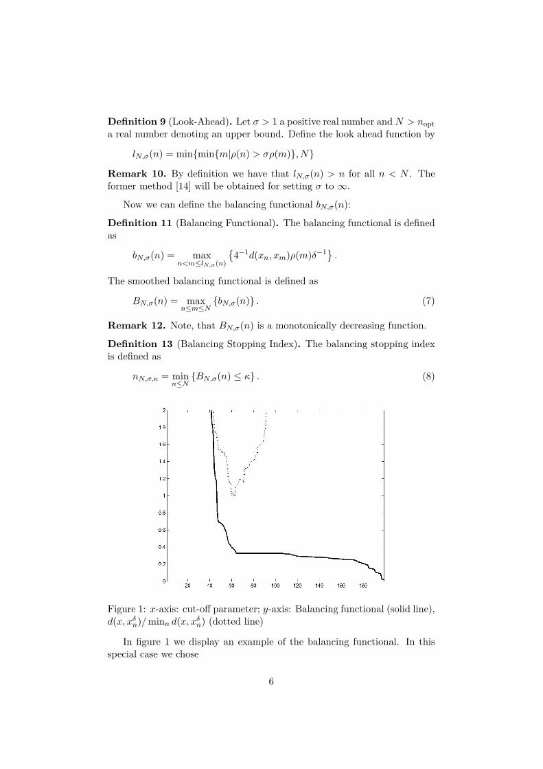
Figure 1: x-axis: cut-off parameter; y-axis: Balancing functional (solid line),d(x, xδ

n)/minn d(x, xδn) (dotted line)

In figure 1 we display an example of the balancing functional. In thisspecial case we chose

6

• X = Y = R200 with standard basis ukk∈1,...,200; d(·, ·) standardl2-norm, i.e. d(x1, x2) = ‖x1 − x2‖2

• A = diag(k−3)

• The Fourier coefficients 〈x, uk〉 of x are independently drawn accordingto N (0, k−5).

• The Fourier coefficients 〈ξ, uk〉 of the noise ξ are independently drawnaccording to N (0, δ2); δ = 10−9.

As regularization method we used spectral cut-off. For determining thebalancing functional we assumed σ = 3. In our experience the displayedgraph is a good prototype for all balancing functionals observed in practice,more or less independent of the regularization method or the used metric.

Lemma 14 (Balancing Lemma). Assume (2), (3) and (6). For the balanc-ing stopping index (8) we obtain

Ed(x, xδnN,σ,κ

)k ≤Ctail(σ)f(nopt, N)(

δ

ρ(N)

)k

exp(−cκl

)+ Cmain(σ)κk OptRate(δ)k (9)

Proof. Define the random variable Ξ by

Ξ = maxnopt≤n≤N

d(x0n, x

δn)ρ(n)δ−1

and define Ωκ = ξ : Ξ ≤ κ and its complement by Ωκ.We will distinguish two cases

Main Behavior: (Ξ ≤ κ, i.e. ξ ∈ Ωκ)For all (n,m) fulfilling nopt ≤ n ≤ m we have

d(xδn, x

δm) ≤ d(x, x0

n) + d(x0n, x

δn) + d(x, x0

m) + d(x0m, x

δm)

≤ ψ(n) +κδ

ρ(n)+ ψ(m) +

κδ

ρ(m)≤ 4κδρ(m)

,

and hence bN,σ(n) ≤ κ. This implies in particular that BN,σ(nopt) ≤ κ andthus nN,σ,κ ≤ nopt (see (7) and (8)).

Now define n0 = nN,σ,κ and nk+1 = lN,σ(nk) stopping if nK > nopt ornK = N . nK is now defined as nK = nopt. Due to the definition of nN,σ,κ

and the monotonicity of BN,σ we obtain for all 0 ≤ k ≤ K that we have

7

BN,σ(nk) ≤ κ. This gives

d(x− xδnN,σ,κ

) ≤ d(x, xδnopt

) +K−1∑k=0

d(xδnk, xδ

nk+1)

≤ Copt OptRate(δ) +K−1∑k=0

4κδρ(nk+1)

≤ Copt OptRate(δ) +4κδ

ρ(nopt)

K−1∑k=0

(σ−1)K−1−k

≤ Copt OptRate(δ) + 4κCopt1

1− σ−1OptRate(δ)

≤ (Cmain(σ))1/kκOptRate(δ).

Tail Behavior: (Ξ > κ, i.e. ξ ∈ Ωκ)Like beforehand we define n0 = nN,σ,κ and nk+1 = lN,σ(nk) stopping if

nK = N . Then we have

d(x, xδnN,σ,κ

) ≤d(x, x0N ) + d(xδ

N , x0N ) +

K−1∑k=0

d(xδnk, xδ

nk+1)

≤ψ(N) +Ξδρ(N)

+4κδρ(N)

11− σ−1

≤ 61

1− σ−1Ξ

δ

ρ(N).

(10)

Using this result we obtain:∫Ωκ

d(x, xδnN,σ,κ

)kdP(ξ) ≤(

31

1− σ−1

δ

ρ(N)

)k ∫Ωκ

ΞkdP(ξ)

≤(

31

1− σ−1

δ

ρ(N)

)k (∫Ωκ

Ξ2kdP(ξ)∫

Ωκ

1dP(ξ))1/2

(11)

Now we estimate the two parts separately.∫Ωκ

Ξ2kdP(ξ) ≤−∫ ∞

κτ2kd

(exp

(−2cτ l

)f(nopt, N)

)≤−

∫ ∞

0τ2kd

(exp

(−2cτ l

)f(nopt, N)

)= −τ2k

(exp

(−2cτ l

)f(nopt, N)

)∣∣∣∞0

+ 2k∫ ∞

0τ2k−1

(exp

(−2cτ l

)f(nopt, N)

)dτ

=2kf(nopt, N)∫ ∞

0τ2k−1

(exp

(−2cτ l

))dτ

≤Clf(nopt, N),

8

and the second factor in (11) is estimated as∫Ωκ

1dP(ξ) ≤ exp(−2cκl

)f(nopt, N).

Hence we get∫Ωκ

ΞkdP(ξ) ≤ Ctail(σ)f(nopt, N)(

δ

ρ(N)

)k

exp(−cκl

).

This yields

Ed(x, xδnN,σ,κ

)k ≤ Ctail(σ)f(nopt, N)(

δ

ρ(N)

)k

exp(−cκl

)+ Cmain(σ)κk OptRate(δ)k.

Theorem 15. Assume (2), (3) and (6). There is a δ0 such that for allδ < δ0 we can choose nopt ≤ N = ρ−1(δ) and have

Ed(x, xδnN,σ,κ

)k ≤ Ctail(σ)f(nopt, N) exp(−cκl

)+ Cmain(σ)κk OptRate(δ)k.

Proof. As A is compact δ/OptRate(δ) → 0 as δ → 0. Hence due to ρ(n+1) ≥ Cspeedρ(n) there is a δ0 s.t. for all δ < δ0 it always holds N = ρ−1(δ) >nopt.

The inequality follows by insertion in (9).

Remark 16. When setting the look-ahead parameter σ to infinity all proofsalso hold provided for all x1, x2, x ∈ X

d(x1, x2)k ≤ cX ,k

(d(x1, x)k + d(x2, x)k

). (12)

for some constant cX ,k. This includes lp with 0 < p < 1 with d(·, ·)p =|| · − · ||pp.

4 The Lepskij Balancing Principle in lp spacesIn the following section we will restrict ourselves to a special situation. Wewill assume that we are operating in separable Hilbert spaces X , Y and(see e.g. [15]) and hence we have a singular value decomposition of thelinear compact operator A : X → Y with the corresponding basis ukk∈Nand vkk∈N and the singular values λkk∈N where the λk are forminga monotonically decreasing sequence tending to zero, where It holds thatAx =

∑∞k=1 λk 〈x, uk〉 vk.

9

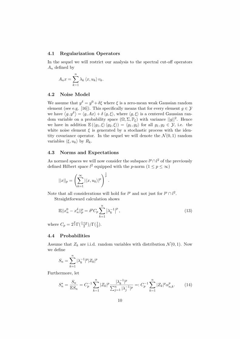
4.1 Regularization Operators

In the sequel we will restrict our analysis to the spectral cut-off operatorsAn defined by

Anx =n∑

k=1

λk 〈x, uk〉 vk.

4.2 Noise Model

We assume that yδ = y0 +δξ where ξ is a zero-mean weak Gaussian randomelement (see e.g. [16]). This specifically means that for every element g ∈ Ywe have

⟨g, yδ

⟩= 〈g,Ax〉+ δ 〈g, ξ〉, where 〈g, ξ〉 is a centered Gaussian ran-

dom variable on a probability space (Ω,Σ,Pξ) with variance ||g||2. Hencewe have in addition E (〈g1, ξ〉 〈g2, ξ〉) = 〈g1, g2〉 for all g1, g2 ∈ Y, i.e. thewhite noise element ξ is generated by a stochastic process with the iden-tity covariance operator. In the sequel we will denote the N (0, 1) randomvariables 〈ξ, uk〉 by Rk.

4.3 Norms and Expectations

As normed spaces we will now consider the subspace lp∩ l2 of the previouslydefined Hilbert space l2 equipped with the p-norm (1 ≤ p ≤ ∞)

||x||p =

( ∞∑k=1

|〈x, uk〉|p) 1

p

.

Note that all considerations will hold for lp and not just for lp ∩ l2.Straightforward calculation shows

E||x0n − xδ

n||pp = δpCp

n∑k=1

∣∣λ−1k

∣∣p , (13)

where Cp = 2p2 Γ(1+p

2 )/Γ(12).

4.4 Probabilities

Assume that Zk are i.i.d. random variables with distribution N (0, 1). Nowwe define

Sn =n∑

k=1

|λ−1k |p|Zk|p

Furthermore, let

S∗n =Sn

ESn= C−1

p

n∑k=1

|Zk|p|λ−1

k |p∑nj=1 |λ

−1j |p

=: C−1p

n∑k=1

|Zk|pαpn,k. (14)

10

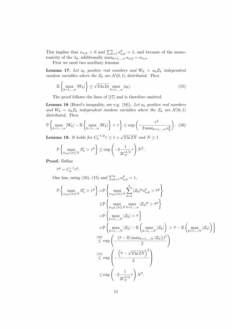
This implies that αn,k > 0 and∑n

k=1 αpn,k = 1, and because of the mono-

tonicity of the λk, additionally maxk=1,...,n αn,k = αn,n.First we need two auxiliary lemmas

Lemma 17. Let ak positive real numbers and Wk = akZk independentrandom variables where the Zk are N (0, 1) distributed. Then

E

maxk=1,...,n

|Wk|≤√

2 ln 2n maxk=1,...,n

|ak|. (15)

The proof follows the lines of [17] and is therefore omitted.

Lemma 18 (Borel’s inequality, see e.g. [18]). Let ak positive real numbersand Wk = akZk independent random variables where the Zk are N (0, 1)distributed. Then

P

maxk=1,...,n

|Wk| − E

maxk=1,...,n

|Wk|> τ

≤ exp

(− τ2

2 maxk=1,...,n a2k

). (16)

Lemma 19. It holds for C−1/pp τ ≥ 1 +

√2 ln 2N and N ≥ 1

P

maxnopt≤n≤N

S∗n > τp

≤ exp

(−2

1

2C1/pp

τ

)N2.

Proof. Define

τp = C−1p τp.

One has, using (16), (15) and∑n

k=1 αpn,k = 1,

P

maxnopt≤n≤N

S∗n > τp

=P

max

nopt≤n≤N

n∑k=1

|Zk|pαpn,k > τp

≤P

maxnopt≤n≤N

maxk=1,...,n

|Zk|p > τp

=P

maxk=1,...,N

|Zk| > τ

=P

maxk=1,...,N

|Zk| − E(

maxk=1,...,N

|Zk|)> τ − E

(max

k=1,...,N|Zk|

)(16)

≤ exp

(−

(τ − E (maxk=1,...,N |Zk|))2

2

)

(15)

≤ exp

−(τ −

√2 ln 2N

)2

2

≤ exp

(−2

1

2C1/pp

τ

)N2.

11

This yields our main theorem:

Theorem 20. Assume that we have an inverse problem in the space lp

fulfilling assumption (2) with Gaussian white noise. Furthermore assumethat it holds κ = 2C1/k

k

√ln 2N for N = ρ−1(δ). Then it holds for a fixed

constant µ

Ed(x, xδnN,σ,κ

)pp ≤ Call(σ)

(lnOptRate(δ)−1

)k OptRate(δ)k.

Proof. Due to C−1/pp κ = 2

√ln 2N ≥ 1 +

√2 ln 2N we can apply the last

lemma and so it holds (3) and (6). Hence the requirements for Lemma 19hold.

Using the same arguments as in [14] we obtain the above result by The-orem 15.

References[1] H. Engl, M. Hanke, A. Neubauer, Regularization of Inverse Problems,

Mathematics and Its Applications, Kluwer Academic Publishers, Dor-drecht, Boston, London, 1996.

[2] A. Tikhonov, V. Arsenin, Solutions of Ill-Posed Problems, Wiley, NewYork, 1977.

[3] B. Hofmann, Regularization of Applied Inverse and Ill-Posed Problems,Teubner, Leipzig, 1986.

[4] O. Scherzer, Taut-string algorithm and regularization programs withG-norm data fit, J. Math. Imaging Vision 23 (2) (2005) 135–143.

[5] M. Nikolova, Analysis of the recovery of edges in images and signalsby minimizing nonconvex regularized least-squares, Multiscale Model.Simul. 4 (3) (2005) 960–991 (electronic).

[6] F. Schöpfer, A. K. Louis, T. Schuster, Nonlinear iterative methods forlinear ill-posed problems in Banach spaces, Inverse Problems 22 (1)(2006) 311–329.

[7] B. A. Mair, F. H. Ruymgaart, Statistical inverse estimation in Hilbertscales, SIAM J. Appl. Math. 56 (5) (1996) 1424–1444.

[8] N. Bissantz, T. Hohage, A. Munk, Consistency and rates of conver-gence of nonlinear Tikhonov regularization with random noise, InverseProblems 20 (2004) 1773–1791.

[9] V. A. Morozov, Methods for solving incorrectly posed problems,Springer-Verlag, New York, 1984.

12

[10] G. Wahba, Practical approximate solutions to linear operator equationswhen the data are noisy, SIAM Journal on Numerical Analysis 14 (4)(1977) 651–667.

[11] P. Hansen, Rank-deficient and discrete ill-posed problems, SIAM Mono-graphs on Mathematical Modeling and Computation, Society for In-dustrial and Applied Mathematics (SIAM), Philadelphia, PA, 1998,numerical aspects of linear inversion.

[12] O. Lepskiı, On a problem of adaptive estimation in Gaussian whitenoise., Theory of Probability and its Applications 35 (3) (1990) 454–466.

[13] P. Mathé, S. Pereverzev, Geometry of linear ill-posed problems in vari-able hilbert spaces, Inverse Problems 19 (3) (2003) 789–803.

[14] F. Bauer, S. Pereverzev, Regularization without preliminary knowledgeof smoothness and error behavior, European J. Appl. Math. 16 (3)(2005) 303 – 317.

[15] W. Rudin, Functional Analysis, McGraw-Hill Series in Higher Mathe-matics, McGraw-Hill Book Company, New York, 1973.

[16] A. V. Skorokhod, Integration in Hilbert space, Springer, Berlin, 1974.

[17] L. Devroye, G. Lugosi, Combinatorial Methods in Density Estimation,Springer Series in Statistics, Springer, New York, 2001.

[18] A. van der Vaart, J. Wellner, Weak Convergence and Empirical Pro-cesses. With Applications to Statistics, Springer Series in Statistics,Springer, New York, 1996.

13