Numerical modeling of wavy stratified two-phase flow in pipes

*Corresponding author. Tel.:#33-05-61-55-97-86; fax:#33-05-61-55-97-60.

E-mail address: [email protected] (A. LineH ).

Chemical Engineering Science 55 (2000) 4681}4697

Numerical modeling of wavy strati"ed two-phase #ow in pipes

Fouad Meknassi!, Rachid Benkirane!, Alain LineH ",*, Lucien Masbernat#!Universite& Sidi Mohamed ben Abdellah, Faculte& des Sciences Dhar-Mehraz, B.P. 1796 Atlas, Fez, Maroc

"Laboratoire d+Inge&nierie des Proce&de& s de l+Environnement, De&partement Ge&nie des Proce&de& s Industriels, Institut National des Sciences Applique&es,Complexe Scientixque de Rangueil, 31077 Toulouse cedex, France

#Institut de Me&canique des Fluides, Institut National Polytechnique de Toulouse, 2 avenue du Professeur Soula, 31400 Toulouse, France

Received 30 March 1999; accepted 2 February 2000

Abstract

The paper presents the numerical modeling of strati"ed #ow in circular cross-section pipe. Due to the geometry of this two-phase#ow, the equations of the problem are derived in bipolar coordinate system. Above the waves, the gas #ow structure isthree dimensional, since secondary #ows are induced by the non-uniformity of boundary conditions related to smooth wall andwavy or rough interface. The secondary #ows being generated by the anisotropy of the turbulence, an algebraic stress model is used inthe gas #ow model. The roughness of the interface is determined from experiments. Given vertical pro"les of longitudinal velocity inthe gas and assuming a classical logarithmic law above the waves, it is possible to determine the magnitude of the interfacialroughness. These experimental values are imposed in the numerical simulations. Given these values, the comparison betweenexperimental pro"les and computed ones is shown to be satisfactory. Hence, the simulations validate the concept of interfacialroughness to account for gas}liquid interactions. Finally, the interfacial roughness are non-dimensionalized following Charnockproposal and its order of magnitude to be imposed in the numerical simulations is given. ( 2000 Elsevier Science Ltd. All rightsreserved.

Keywords: Strati"ed #ow; Waves, Interfacial transfer; Secondary #ow

1. Introduction

The main problem of the modeling of strati"ed two-phase #ow in pipes is related to the modeling of mo-mentum transfer for each phase at the wall and betweenthe two phases at the interface. In a global approach ofthe problem (Taitel & Dukler, 1976a, b), it is then neces-sary to propose three closure relations to express mo-mentum transfer coe$cients. Given gas and liquid #owrates, the global determination of both pressure drop andphase distribution (gas hold up) will strongly depend onthe momentum transfer modeling.

The wall friction factor in the gas phase is generallywell predicted by extrapolating classical relations derivedin single phase #ow (LineH & Fabre, 1996). The wallfriction factor in the liquid phase can be extrapolatedfrom single-phase relation as long as the liquid fraction is

not too small. However, Cheremisino! and Davies(1979), Rosant (1983) and Andritsos (1986) proposed spe-ci"c empirical correlations to improve the modeling ofthe wall friction factor in thin liquid "lms. Indeed, the keystone of the modeling lies in the expression of the inter-facial momentum transfer which is closely related to thedeformation of the gas}liquid interface. For smoothstrati"ed #ow, there is no problem to express the corre-sponding smooth friction factor. For wavy strati"ed #ow,two approaches can be followed: on the one hand, onecan propose a global empirical correlation for the inter-facial friction factor; on the other hand, one can considerthe analogy to shear #ow above a rough interface andpropose at least an empirical correlation for the inter-facial roughness. Many authors followed the "rstapproach; in this scope, the correlation proposed byAndritsos and Hanratty (1987) is probably the moste$cient one. The very "rst attempts to correlate theinterfacial roughness mentioned in the second approachare due to Charnock (1955), who introduced a Froudenumber relating the roughness to the wind velocity. Sinai(1985) reviewed this second approach. At this point, the

0009-2509/00/$ - see front matter ( 2000 Elsevier Science Ltd. All rights reserved.PII: S 0 0 0 9 - 2 5 0 9 ( 0 0 ) 0 0 0 7 0 - 1

only way to improve the understanding and the modelingof two-phase strati"ed #ow is based on the local analysisof the phenomena.

In a general review on phenomenological understand-ing of gas}liquid separated #ows, Hanratty andMcCready (1992) highlighted the necessity of a betterknowledge of small-scale interactions to improve themacroscopic behavior description. In the present paper,we develop a local approach. In particular, we refer totwo experimental studies after Strand (1993) and Lopez(1994), who measured interfacial deformations togetherwith spatial distributions of velocity "eld in air}waterstrati"ed #ow in horizontal or slightly inclined pipes.A "rst instructive experimental result is that above thewaves, the vertical pro"le of longitudinal velocity can be"tted by a classical logarithmic law. It is then possible toestimate the interfacial roughness from experiments.A second instructive result is that secondary #ows canbe observed both over and below the waves. These sec-ondary #ows have been studied in the past (Suzanne,1985; Banat, 1985; Magnaudet, 1989; Benkirane, 1990;Soualmia, 1993; Strand, 1993). It is now well acceptedthat the secondary #ows in the gas phase are governed bythe anisotropy of the turbulence (Jayanti, Wilke, Clarke& Hewitt, 1989, LineH , Masbernat & Soualmia, 1996). Theanisotropy of the turbulence in the gas phase is itselfinduced by the non-uniformity of the boundary condi-tions : the wall is smooth and the wavy interface is rough.In a previous attempt of numerical modeling of strati"ed#ow in rectangular channel, LineH et al. (1996) focused oninterfacial interactions and secondary #ows. In the pres-ent study in circular cross-section pipes, the same inter-facial interactions are considered to explain secondary#ows. Given these mechanisms, we focus in this paper onthe ability of the interfacial roughness concept to repro-duce the secondary #ows observed in experiments.Therefore, the 3D velocity "eld is numerically computed,given appropriate physical model (Sections 2.2 and 2.3).The computed pro"les are compared to di!erent experi-mental results.

Indeed, in the present simulations, we will impose theinterfacial roughness according to experiments and,given a model of anisotropic turbulence in the gas phase,we will compare experimental and computed velocity"elds. Since secondary #ows are the signature of inter-facial interactions, the correctness of velocity distributionwill validate the interfacial roughness estimation. In fact,the secondary #ows modify strongly the longitudinalvelocity distribution. The comparison between experi-mental and numerical pro"les of the longitudinal velocitywill then be analyzed.

The present study will be centered on the problem ofthe #ow in the gas. The main objective is to analyze theinterfacial roughness concept. The "rst important issue isto account for secondary #ows induced by the waves inthe gas phase. If we correctly account for the secondary

#ows, it will imply that the interfacial roughness is cor-rectly estimated. Then the question to be addressed ishow to estimate the interfacial roughness ? This last pointwill not be answered in this paper; we will brie#y presentsome trends at the end of the paper. Most of the resultswill concern the gas #ow. However, some results will alsobe given in the liquid.

2. Strati5ed 6ow modeling

Di!erent authors have published attempts of localmodeling of strati"ed two-phase #ow. Akai, Inoue andAoki (1981) published a "rst 1D model above and belowthe waves. Shoham and Taitel (1984) were interested inthe velocity distribution in the liquid phase in inclinedpipes. The 2D model they used was relatively simpli"ed.Issa (1988) extended the work of Akai et al. (1981) to 2Dcase and solved the problem of strati"ed #ow usinga classical (k, e) two-equation model of turbulence. Con-sequently, he could not reproduce secondary #ows sincethe (k, e) is basically isotropic. Comparatively, Benkirane,LineH and Masbernat (1990) and Soualmia (1993) im-proved the numerical simulation of secondary #owsabove and below the waves in a rectangular cross-section#ow.

The present contribution accounts for the same kind ofphysical modeling of interfacial interactions in strati"ed#ow, including the mechanism generating secondary#ows and simulates these phenomena in a circular cross-section pipe. A numerical code has been developed andwill be shortly presented in the paper. The coordinatesystem is "rstly recalled (Section 2.1). The complete set ofequations in the gas phase is then developed and com-mented (Section 2.2). The modeling in the liquid phase isbrie#y presented. Some informations are "nally givenconcerning numerical methods.

2.1. Bipolar coordinate system

Given x the longitudinal axis, the cross #ow section isin the plane (y, z). Following previous studies, (Shoham& Taitel, 1984; Issa, 1988) bipolar coordinates are usedand de"ned by (g, m). The curvilinear coordinates arerelated to cartesian coordinates by the expressions

y"c sin h(g)

cosh(g)!cos(m), (1a)

z"c sin(m)

cosh(g)!cos(m), (1b)

where the length c is de"ned as

c"(R!d) sin(c), (2)

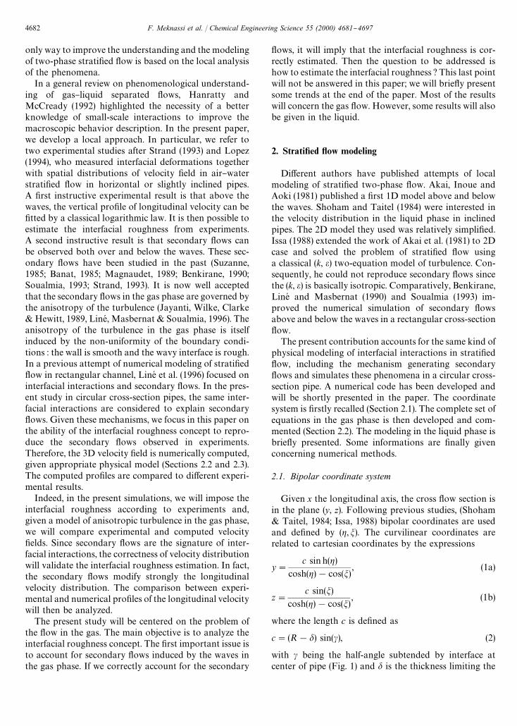
with c being the half-angle subtended by interface atcenter of pipe (Fig. 1) and d is the thickness limiting the

4682 F. Meknassi et al. / Chemical Engineering Science 55 (2000) 4681}4697

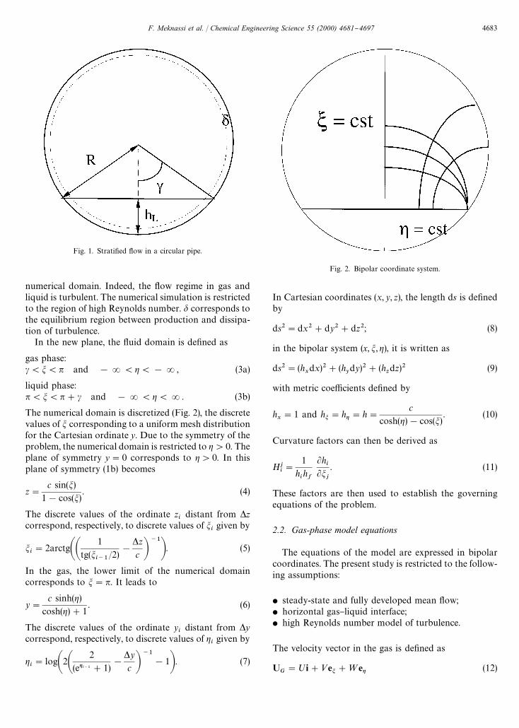
Fig. 1. Strati"ed #ow in a circular pipe.

Fig. 2. Bipolar coordinate system.

numerical domain. Indeed, the #ow regime in gas andliquid is turbulent. The numerical simulation is restrictedto the region of high Reynolds number. d corresponds tothe equilibrium region between production and dissipa-tion of turbulence.

In the new plane, the #uid domain is de"ned as

gas phase:c(m(n and !R(g(!R, (3a)

liquid phase:n(m(n#c and !R(g(R. (3b)

The numerical domain is discretized (Fig. 2), the discretevalues of m corresponding to a uniform mesh distributionfor the Cartesian ordinate y. Due to the symmetry of theproblem, the numerical domain is restricted to g'0. Theplane of symmetry y"0 corresponds to g'0. In thisplane of symmetry (1b) becomes

z"c sin(m)

1!cos(m). (4)

The discrete values of the ordinate zi

distant from *zcorrespond, respectively, to discrete values of m

igiven by

mi"2arctgAA

1

tg(mi~1

/2)!

*z

c B~1

B. (5)

In the gas, the lower limit of the numerical domaincorresponds to m"n. It leads to

y"c sinh(g)

cosh(g)#1. (6)

The discrete values of the ordinate yi

distant from *ycorrespond, respectively, to discrete values of g

igiven by

gi"logA2A

2

(egi~1#1)!

*y

c B~1

!1B. (7)

In Cartesian coordinates (x, y, z), the length ds is de"nedby

ds2"dx2#dy2#dz2; (8)

in the bipolar system (x, m, g), it is written as

ds2"(hxdx)2#(h

ydy)2#(h

zdz)2 (9)

with metric coe$cients de"ned by

hx"1 and hm"hg"h"

c

cosh(g)!cos(m). (10)

Curvature factors can then be derived as

Hji"

1

hihf

Lhi

Lmj

. (11)

These factors are then used to establish the governingequations of the problem.

2.2. Gas-phase model equations

The equations of the model are expressed in bipolarcoordinates. The present study is restricted to the follow-ing assumptions:

f steady-state and fully developed mean #ow;f horizontal gas}liquid interface;f high Reynolds number model of turbulence.

The velocity vector in the gas is de"ned as

UG";i#<em#=eg (12)

F. Meknassi et al. / Chemical Engineering Science 55 (2000) 4681}4697 4683

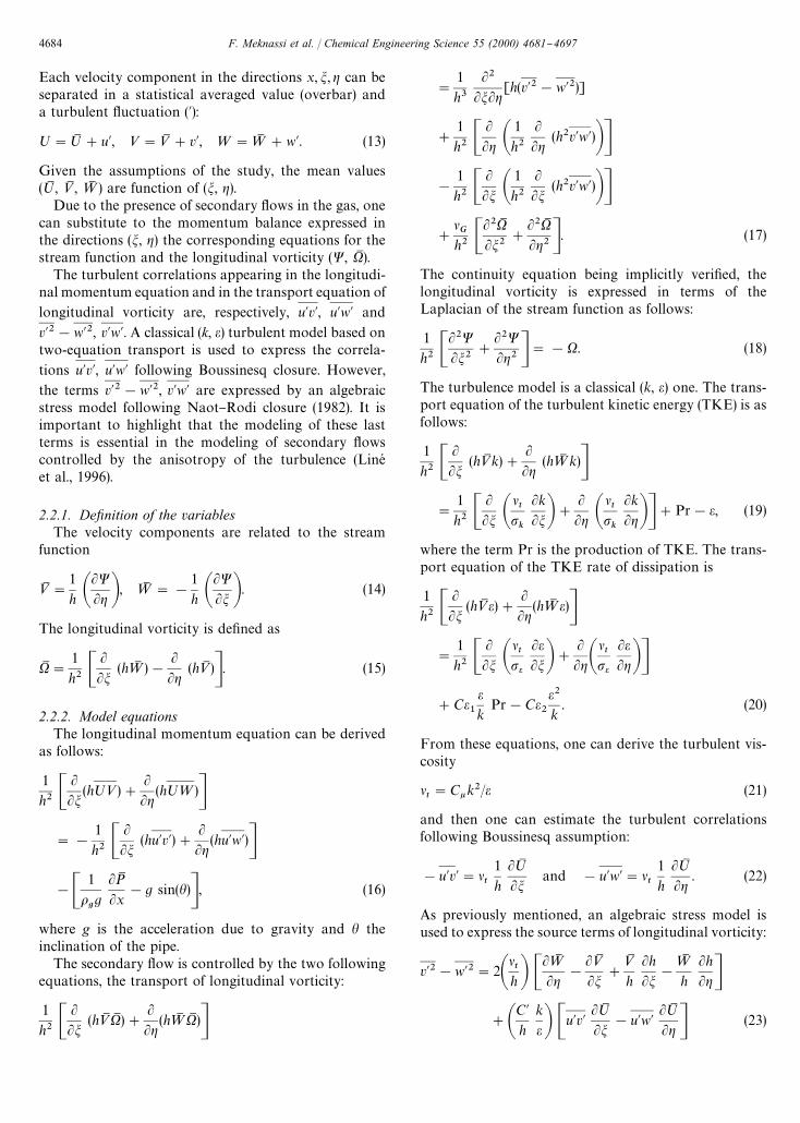
Each velocity component in the directions x, m, g can beseparated in a statistical averaged value (overbar) anda turbulent #uctuation (@):

;";M #u@, <"<M #v@, ="=M #w@. (13)

Given the assumptions of the study, the mean values(;M , <M , =M ) are function of (m, g).

Due to the presence of secondary #ows in the gas, onecan substitute to the momentum balance expressed inthe directions (m, g) the corresponding equations for thestream function and the longitudinal vorticity (W, XM ).

The turbulent correlations appearing in the longitudi-nal momentum equation and in the transport equation of

longitudinal vorticity are, respectively, u@v@, u@w@ and

v@2!w@2, v@w@. A classical (k, e) turbulent model based ontwo-equation transport is used to express the correla-

tions u@v@, u@w@ following Boussinesq closure. However,

the terms v@2!w@2, v@w@ are expressed by an algebraicstress model following Naot}Rodi closure (1982). It isimportant to highlight that the modeling of these lastterms is essential in the modeling of secondary #owscontrolled by the anisotropy of the turbulence (LineHet al., 1996).

2.2.1. Dexnition of the variablesThe velocity components are related to the stream

function

<M "1

h ALW

Lg B, =M "!

1

h ALW

Lm B. (14)

The longitudinal vorticity is de"ned as

XM "1

h2 CLLm

(h=M )!LLg

(h<M )D. (15)

2.2.2. Model equationsThe longitudinal momentum equation can be derived

as follows:

1

h2 CLLm

(h;<)#LLg

(h;=)D"!

1

h2 CLLm

(hu@v@)#LLg

(hu@w@)D!C

1

ogg

LPMLx

!g sin(h)D, (16)

where g is the acceleration due to gravity and h theinclination of the pipe.

The secondary #ow is controlled by the two followingequations, the transport of longitudinal vorticity:

1

h2 CLLm

(h<M XM )#LLg

(h=M XM )D

"

1

h3L2

LmLg[h(v@2!w@2)]

#

1

h2 CLLg A

1

h2

LLg

(h2v@w@)BD!

1

h2 CLLm A

1

h2

LLm

(h2v@w@)BD#

lG

h2 CL2XMLm2

#

L2XMLg2 D. (17)

The continuity equation being implicitly veri"ed, thelongitudinal vorticity is expressed in terms of theLaplacian of the stream function as follows:

1

h2 CL2W

Lm2#

L2WLg2 D"!X. (18)

The turbulence model is a classical (k, e) one. The trans-port equation of the turbulent kinetic energy (TKE) is asfollows:

1

h2 CLLm

(h<M k)#LLg

(h=M k)D"

1

h2 CLLm A

lt

pk

Lk

LmB#LLg A

lt

pk

Lk

LgBD#Pr!e, (19)

where the term Pr is the production of TKE. The trans-port equation of the TKE rate of dissipation is

1

h2 CLLm

(h<M e)#LLg

(h=M e)D"

1

h2 CLLm A

lt

pe

LeLmB#

LLgA

lt

pe

LeLgBD

#Ce1

ek

Pr!Ce2

e2k

. (20)

From these equations, one can derive the turbulent vis-cosity

lt"Ckk2/e (21)

and then one can estimate the turbulent correlationsfollowing Boussinesq assumption:

!u@v@"lt

1

h

L;MLm

and !u@w@"lt

1

h

L;MLg

. (22)

As previously mentioned, an algebraic stress model isused to express the source terms of longitudinal vorticity:

v@2!w@2"2Alth B C

L=MLg

!

L<MLm

#

<Mh

Lh

Lm!

=Mh

Lh

LgD#A

C@h

k

eB Cu@v@L;MLm

!u@w@L;MLg D (23)


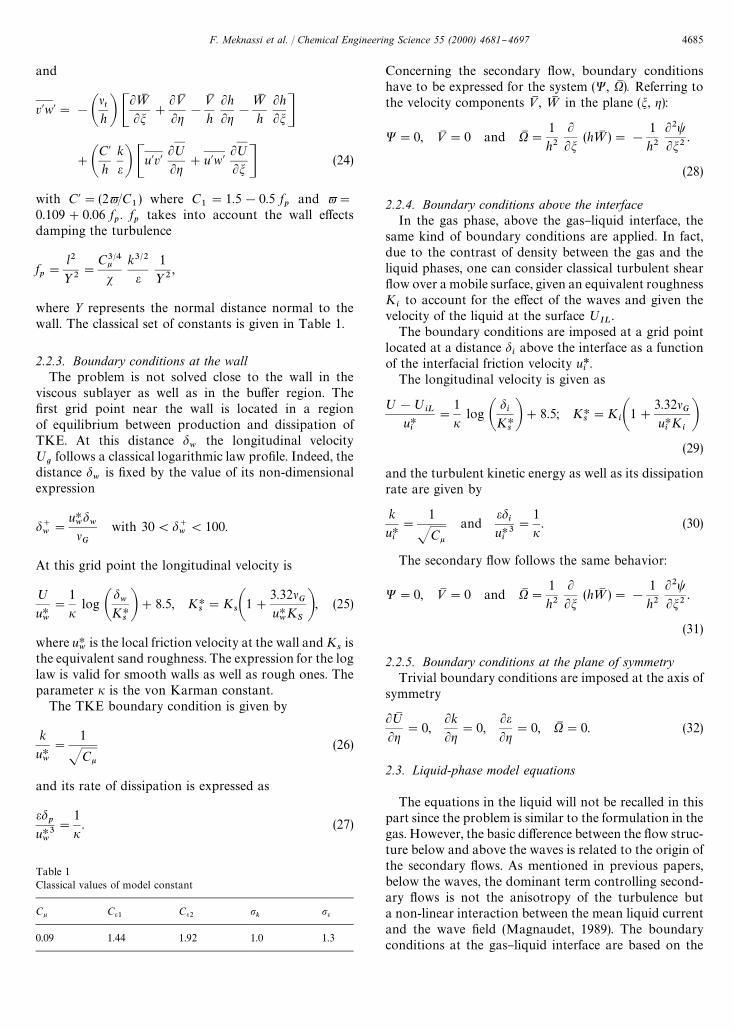
Table 1Classical values of model constant

Ck Ce1 Ce2 pk

pe

0.09 1.44 1.92 1.0 1.3

and

v@w@"!Alth B C

L=MLm

#

L<MLg

!

<Mh

Lh

Lg!

=Mh

Lh

LmD#A

C@h

k

eB Cu@v@L;Lg

#u@w@L;Lm D (24)

with C@"(2-/C1) where C

1"1.5!0.5 f

pand -"

0.109#0.06 fp. f

ptakes into account the wall e!ects

damping the turbulence

fp"

l2

>2"

C3@4ks

k3@2

e1

>2,

where Y represents the normal distance normal to thewall. The classical set of constants is given in Table 1.

2.2.3. Boundary conditions at the wallThe problem is not solved close to the wall in the

viscous sublayer as well as in the bu!er region. The"rst grid point near the wall is located in a regionof equilibrium between production and dissipation ofTKE. At this distance d

wthe longitudinal velocity

;gfollows a classical logarithmic law pro"le. Indeed, the

distance dw

is "xed by the value of its non-dimensionalexpression

d`w"

uHwdw

lG

with 30(d`w(100.

At this grid point the longitudinal velocity is

;

uHw

"

1

ilog A

dw

KHsB#8.5, KH

s"K

sA1#3.32l

GuHwK

SB, (25)

where uHw

is the local friction velocity at the wall and Ksis

the equivalent sand roughness. The expression for the loglaw is valid for smooth walls as well as rough ones. Theparameter i is the von Karman constant.

The TKE boundary condition is given by

k

uHw

"

1

JCk(26)

and its rate of dissipation is expressed as

edp

uH3w

"

1

i. (27)

Concerning the secondary #ow, boundary conditionshave to be expressed for the system (W, XM ). Referring tothe velocity components <M , =M in the plane (m, g):

W"0, <M "0 and XM "1

h2LLm

(h=M )"!

1

h2L2tLm2

.

(28)

2.2.4. Boundary conditions above the interfaceIn the gas phase, above the gas}liquid interface, the

same kind of boundary conditions are applied. In fact,due to the contrast of density between the gas and theliquid phases, one can consider classical turbulent shear#ow over a mobile surface, given an equivalent roughnessK

ito account for the e!ect of the waves and given the

velocity of the liquid at the surface ;IL

.The boundary conditions are imposed at a grid point

located at a distance diabove the interface as a function

of the interfacial friction velocity u*i.

The longitudinal velocity is given as

;!;iL

uHi

"

1

ilog A

di

KHsB#8.5; KH

s"K

iA1#3.32l

GuHiK

iB

(29)

and the turbulent kinetic energy as well as its dissipationrate are given by

k

uHi

"

1

JCkand

edi

uH3i

"

1

i. (30)

The secondary #ow follows the same behavior:

W"0, <M "0 and XM "1

h2LLm

(h=M )"!

1

h2L2tLm2

.

(31)

2.2.5. Boundary conditions at the plane of symmetryTrivial boundary conditions are imposed at the axis of

symmetry

L;MLg

"0,Lk

Lg"0,

LeLg

"0, XM "0. (32)

2.3. Liquid-phase model equations

The equations in the liquid will not be recalled in thispart since the problem is similar to the formulation in thegas. However, the basic di!erence between the #ow struc-ture below and above the waves is related to the origin ofthe secondary #ows. As mentioned in previous papers,below the waves, the dominant term controlling second-ary #ows is not the anisotropy of the turbulence buta non-linear interaction between the mean liquid currentand the wave "eld (Magnaudet, 1989). The boundaryconditions at the gas}liquid interface are based on the


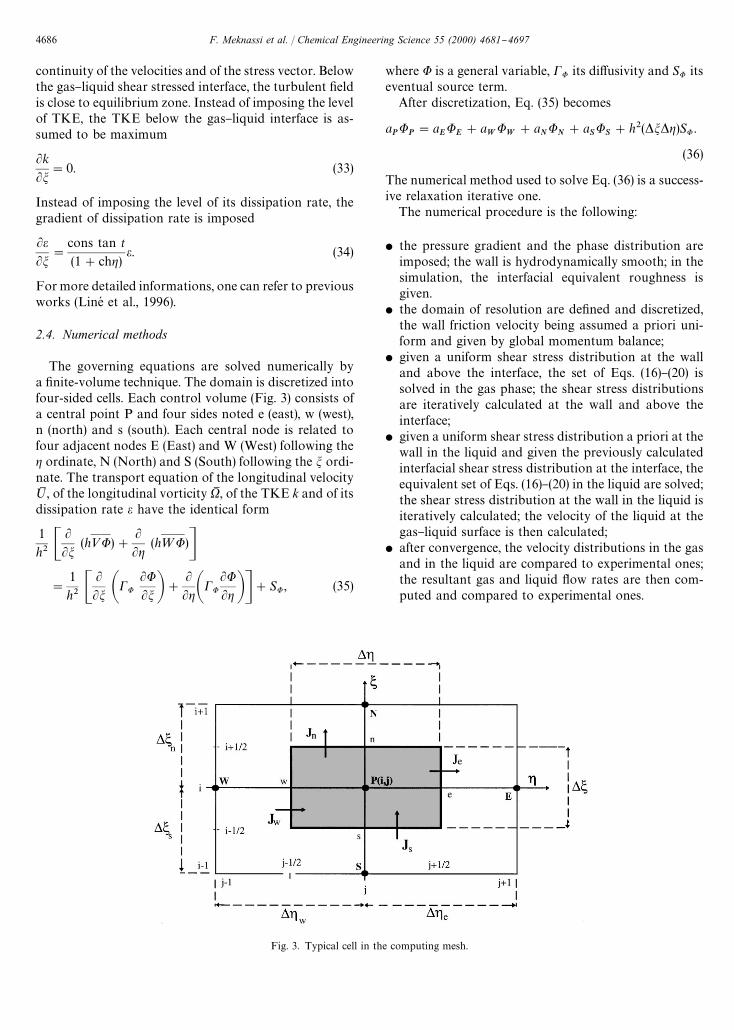
Fig. 3. Typical cell in the computing mesh.

continuity of the velocities and of the stress vector. Belowthe gas}liquid shear stressed interface, the turbulent "eldis close to equilibrium zone. Instead of imposing the levelof TKE, the TKE below the gas}liquid interface is as-sumed to be maximum

Lk

Lm"0. (33)

Instead of imposing the level of its dissipation rate, thegradient of dissipation rate is imposed

LeLm

"

cons tan t

(1#chg)e. (34)

For more detailed informations, one can refer to previousworks (LineH et al., 1996).

2.4. Numerical methods

The governing equations are solved numerically bya "nite-volume technique. The domain is discretized intofour-sided cells. Each control volume (Fig. 3) consists ofa central point P and four sides noted e (east), w (west),n (north) and s (south). Each central node is related tofour adjacent nodes E (East) and W (West) following theg ordinate, N (North) and S (South) following the m ordi-nate. The transport equation of the longitudinal velocity;M , of the longitudinal vorticity XM , of the TKE k and of itsdissipation rate e have the identical form

1

h2 CLLm

(h<U)#LLg

(h=U)D"

1

h2 CLLm ACU

LU

Lm B#LLgACU

LU

Lg BD#SU , (35)

where U is a general variable, CU its di!usivity and SU itseventual source term.

After discretization, Eq. (35) becomes

aPU

P"a

EU

E#a

WU

W#a

NU

N#a

SU

S#h2(*m*g)SU .

(36)

The numerical method used to solve Eq. (36) is a success-ive relaxation iterative one.

The numerical procedure is the following:

f the pressure gradient and the phase distribution areimposed; the wall is hydrodynamically smooth; in thesimulation, the interfacial equivalent roughness isgiven.

f the domain of resolution are de"ned and discretized,the wall friction velocity being assumed a priori uni-form and given by global momentum balance;

f given a uniform shear stress distribution at the walland above the interface, the set of Eqs. (16)}(20) issolved in the gas phase; the shear stress distributionsare iteratively calculated at the wall and above theinterface;

f given a uniform shear stress distribution a priori at thewall in the liquid and given the previously calculatedinterfacial shear stress distribution at the interface, theequivalent set of Eqs. (16)}(20) in the liquid are solved;the shear stress distribution at the wall in the liquid isiteratively calculated; the velocity of the liquid at thegas}liquid surface is then calculated;

f after convergence, the velocity distributions in the gasand in the liquid are compared to experimental ones;the resultant gas and liquid #ow rates are then com-puted and compared to experimental ones.


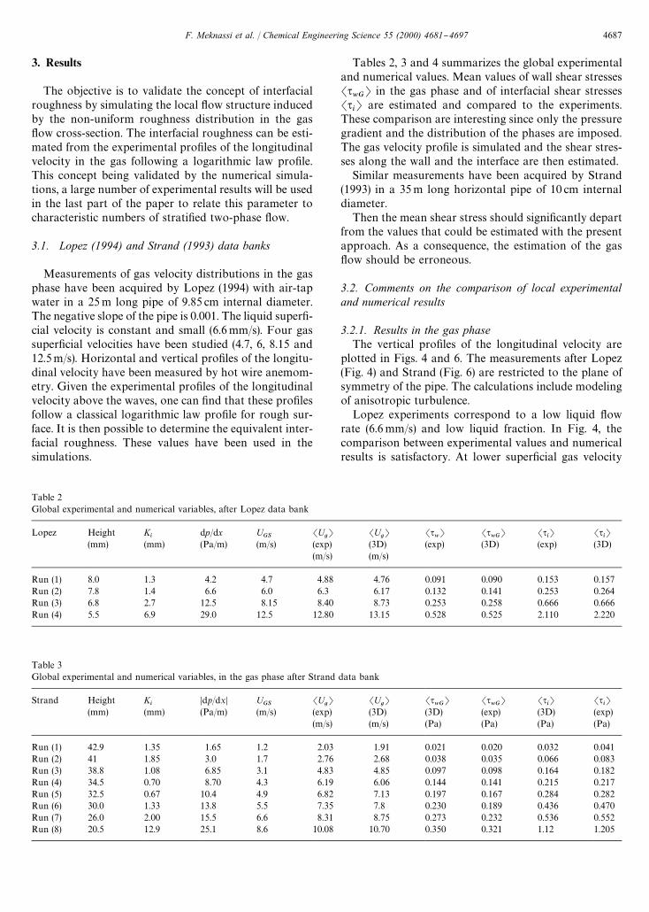
Table 3Global experimental and numerical variables, in the gas phase after Strand data bank

Strand Height Ki

Ddp/dxD UGS

SUgT SU

gT Ss

wGT Ss

wGT Ss

iT Ss

iT

(mm) (mm) (Pa/m) (m/s) (exp) (3D) (3D) (exp) (3D) (exp)(m/s) (m/s) (Pa) (Pa) (Pa) (Pa)

Run (1) 42.9 1.35 1.65 1.2 2.03 1.91 0.021 0.020 0.032 0.041Run (2) 41 1.85 3.0 1.7 2.76 2.68 0.038 0.035 0.066 0.083Run (3) 38.8 1.08 6.85 3.1 4.83 4.85 0.097 0.098 0.164 0.182Run (4) 34.5 0.70 8.70 4.3 6.19 6.06 0.144 0.141 0.215 0.217Run (5) 32.5 0.67 10.4 4.9 6.82 7.13 0.197 0.167 0.284 0.282Run (6) 30.0 1.33 13.8 5.5 7.35 7.8 0.230 0.189 0.436 0.470Run (7) 26.0 2.00 15.5 6.6 8.31 8.75 0.273 0.232 0.536 0.552Run (8) 20.5 12.9 25.1 8.6 10.08 10.70 0.350 0.321 1.12 1.205

Table 2Global experimental and numerical variables, after Lopez data bank

Lopez Height Ki

dp/dx UGS

SUgT SU

gT Ss

wT Ss

wGT Ss

iT Ss

iT

(mm) (mm) (Pa/m) (m/s) (exp) (3D) (exp) (3D) (exp) (3D)(m/s) (m/s)

Run (1) 8.0 1.3 4.2 4.7 4.88 4.76 0.091 0.090 0.153 0.157Run (2) 7.8 1.4 6.6 6.0 6.3 6.17 0.132 0.141 0.253 0.264Run (3) 6.8 2.7 12.5 8.15 8.40 8.73 0.253 0.258 0.666 0.666Run (4) 5.5 6.9 29.0 12.5 12.80 13.15 0.528 0.525 2.110 2.220

3. Results

The objective is to validate the concept of interfacialroughness by simulating the local #ow structure inducedby the non-uniform roughness distribution in the gas#ow cross-section. The interfacial roughness can be esti-mated from the experimental pro"les of the longitudinalvelocity in the gas following a logarithmic law pro"le.This concept being validated by the numerical simula-tions, a large number of experimental results will be usedin the last part of the paper to relate this parameter tocharacteristic numbers of strati"ed two-phase #ow.

3.1. Lopez (1994) and Strand (1993) data banks

Measurements of gas velocity distributions in the gasphase have been acquired by Lopez (1994) with air-tapwater in a 25m long pipe of 9.85 cm internal diameter.The negative slope of the pipe is 0.001. The liquid super"-cial velocity is constant and small (6.6mm/s). Four gassuper"cial velocities have been studied (4.7, 6, 8.15 and12.5m/s). Horizontal and vertical pro"les of the longitu-dinal velocity have been measured by hot wire anemom-etry. Given the experimental pro"les of the longitudinalvelocity above the waves, one can "nd that these pro"lesfollow a classical logarithmic law pro"le for rough sur-face. It is then possible to determine the equivalent inter-facial roughness. These values have been used in thesimulations.

Tables 2, 3 and 4 summarizes the global experimentaland numerical values. Mean values of wall shear stressesSs

wGT in the gas phase and of interfacial shear stresses

SsiT are estimated and compared to the experiments.

These comparison are interesting since only the pressuregradient and the distribution of the phases are imposed.The gas velocity pro"le is simulated and the shear stres-ses along the wall and the interface are then estimated.

Similar measurements have been acquired by Strand(1993) in a 35m long horizontal pipe of 10 cm internaldiameter.

Then the mean shear stress should signi"cantly departfrom the values that could be estimated with the presentapproach. As a consequence, the estimation of the gas#ow should be erroneous.

3.2. Comments on the comparison of local experimentaland numerical results

3.2.1. Results in the gas phaseThe vertical pro"les of the longitudinal velocity are

plotted in Figs. 4 and 6. The measurements after Lopez(Fig. 4) and Strand (Fig. 6) are restricted to the plane ofsymmetry of the pipe. The calculations include modelingof anisotropic turbulence.

Lopez experiments correspond to a low liquid #owrate (6.6mm/s) and low liquid fraction. In Fig. 4, thecomparison between experimental values and numericalresults is satisfactory. At lower super"cial gas velocity


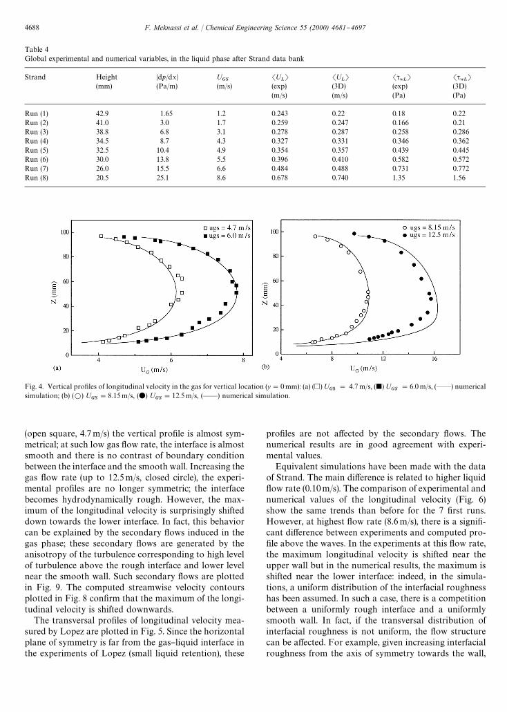
Table 4Global experimental and numerical variables, in the liquid phase after Strand data bank

Strand Height Ddp/dxD UGS

SULT SU

LT Ss

wLT Ss

wLT

(mm) (Pa/m) (m/s) (exp) (3D) (exp) (3D)(m/s) (m/s) (Pa) (Pa)

Run (1) 42.9 1.65 1.2 0.243 0.22 0.18 0.22Run (2) 41.0 3.0 1.7 0.259 0.247 0.166 0.21Run (3) 38.8 6.8 3.1 0.278 0.287 0.258 0.286Run (4) 34.5 8.7 4.3 0.327 0.331 0.346 0.362Run (5) 32.5 10.4 4.9 0.354 0.357 0.439 0.445Run (6) 30.0 13.8 5.5 0.396 0.410 0.582 0.572Run (7) 26.0 15.5 6.6 0.484 0.488 0.731 0.772Run (8) 20.5 25.1 8.6 0.678 0.740 1.35 1.56

Fig. 4. Vertical pro"les of longitudinal velocity in the gas for vertical location (y"0mm): (a) (h) UGS

" 4.7 m/s, (j) UGS

"6.0 m/s, (**) numericalsimulation; (b) (L) U

GS"8.15m/s, (v) U

GS"12.5m/s, (**) numerical simulation.

(open square, 4.7m/s) the vertical pro"le is almost sym-metrical; at such low gas #ow rate, the interface is almostsmooth and there is no contrast of boundary conditionbetween the interface and the smooth wall. Increasing thegas #ow rate (up to 12.5m/s, closed circle), the experi-mental pro"les are no longer symmetric; the interfacebecomes hydrodynamically rough. However, the max-imum of the longitudinal velocity is surprisingly shifteddown towards the lower interface. In fact, this behaviorcan be explained by the secondary #ows induced in thegas phase; these secondary #ows are generated by theanisotropy of the turbulence corresponding to high levelof turbulence above the rough interface and lower levelnear the smooth wall. Such secondary #ows are plottedin Fig. 9. The computed streamwise velocity contoursplotted in Fig. 8 con"rm that the maximum of the longi-tudinal velocity is shifted downwards.

The transversal pro"les of longitudinal velocity mea-sured by Lopez are plotted in Fig. 5. Since the horizontalplane of symmetry is far from the gas}liquid interface inthe experiments of Lopez (small liquid retention), these

pro"les are not a!ected by the secondary #ows. Thenumerical results are in good agreement with experi-mental values.

Equivalent simulations have been made with the dataof Strand. The main di!erence is related to higher liquid#ow rate (0.10m/s). The comparison of experimental andnumerical values of the longitudinal velocity (Fig. 6)show the same trends than before for the 7 "rst runs.However, at highest #ow rate (8.6m/s), there is a signi"-cant di!erence between experiments and computed pro-"le above the waves. In the experiments at this #ow rate,the maximum longitudinal velocity is shifted near theupper wall but in the numerical results, the maximum isshifted near the lower interface: indeed, in the simula-tions, a uniform distribution of the interfacial roughnesshas been assumed. In such a case, there is a competitionbetween a uniformly rough interface and a uniformlysmooth wall. In fact, if the transversal distribution ofinterfacial roughness is not uniform, the #ow structurecan be a!ected. For example, given increasing interfacialroughness from the axis of symmetry towards the wall,


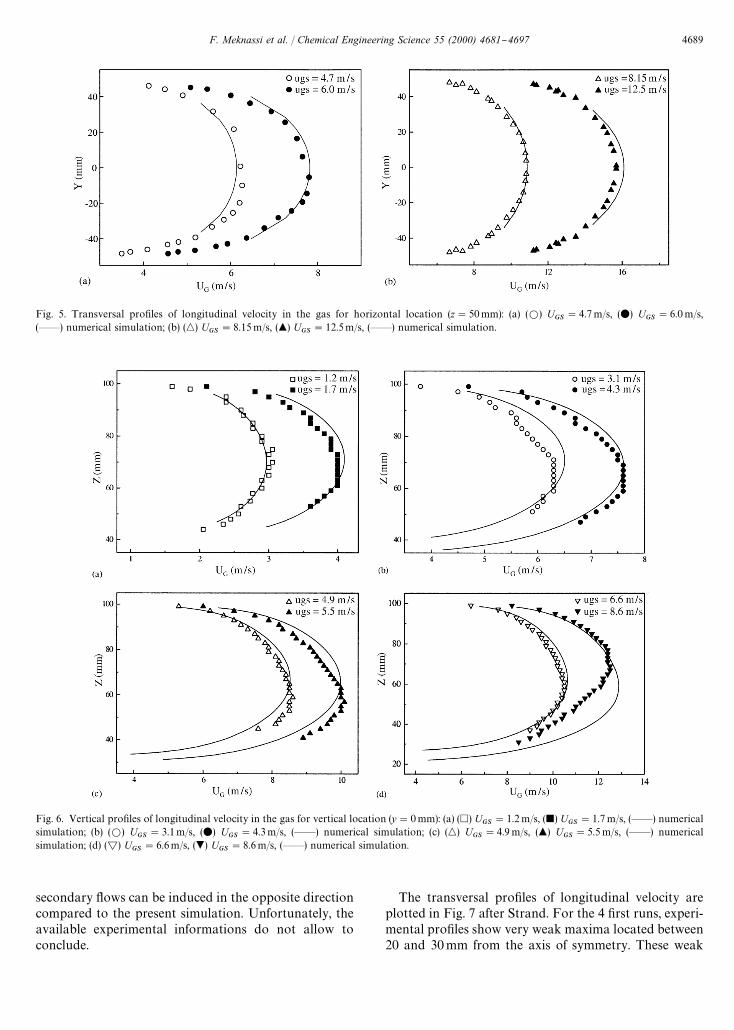
Fig. 5. Transversal pro"les of longitudinal velocity in the gas for horizontal location (z"50mm): (a) (L) UGS

"4.7 m/s, (v) UGS

"6.0 m/s,(**) numerical simulation; (b) (n) U

GS"8.15m/s, (m) U

GS"12.5m/s, (**) numerical simulation.

Fig. 6. Vertical pro"les of longitudinal velocity in the gas for vertical location (y"0mm): (a) (h) UGS

"1.2 m/s, (j) UGS

"1.7 m/s, (**) numericalsimulation; (b) (L) U

GS"3.1m/s, (v) U

GS"4.3m/s, (**) numerical simulation; (c) (n) U

GS"4.9 m/s, (m) U

GS"5.5 m/s, (**) numerical

simulation; (d) (£) UGS

"6.6m/s, (.) UGS

"8.6m/s, (**) numerical simulation.

secondary #ows can be induced in the opposite directioncompared to the present simulation. Unfortunately, theavailable experimental informations do not allow toconclude.

The transversal pro"les of longitudinal velocity areplotted in Fig. 7 after Strand. For the 4 "rst runs, experi-mental pro"les show very weak maxima located between20 and 30mm from the axis of symmetry. These weak


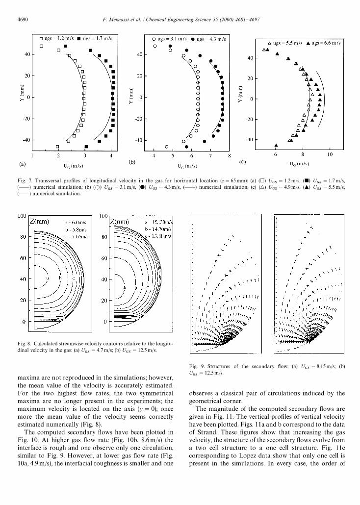
Fig. 7. Transversal pro"les of longitudinal velocity in the gas for horizontal location (z"65mm): (a) (h) UGS

"1.2m/s, (j) UGS

"1.7 m/s,(**) numerical simulation; (b) (L) U

GS"3.1m/s, (v) U

GS"4.3m/s, (**) numerical simulation; (c) (n) U

GS"4.9m/s, (m) U

GS"5.5 m/s,

(**) numerical simulation.

Fig. 8. Calculated streamwise velocity contours relative to the longitu-dinal velocity in the gas: (a) U

GS"4.7m/s; (b) U

GS"12.5 m/s.

Fig. 9. Structures of the secondary #ow: (a) UGS

"8.15m/s; (b)U

GS"12.5m/s.

maxima are not reproduced in the simulations; however,the mean value of the velocity is accurately estimated.For the two highest #ow rates, the two symmetricalmaxima are no longer present in the experiments; themaximum velocity is located on the axis (y"0); oncemore the mean value of the velocity seems correctlyestimated numerically (Fig. 8).

The computed secondary #ows have been plotted inFig. 10. At higher gas #ow rate (Fig. 10b, 8.6m/s) theinterface is rough and one observe only one circulation,similar to Fig. 9. However, at lower gas #ow rate (Fig.10a, 4.9m/s), the interfacial roughness is smaller and one

observes a classical pair of circulations induced by thegeometrical corner.

The magnitude of the computed secondary #ows aregiven in Fig. 11. The vertical pro"les of vertical velocityhave been plotted. Figs. 11a and b correspond to the dataof Strand. These "gures show that increasing the gasvelocity, the structure of the secondary #ows evolve froma two cell structure to a one cell structure. Fig. 11ccorresponding to Lopez data show that only one cell ispresent in the simulations. In every case, the order of


Fig. 11. Vertical pro"les of vertical velocity in the gas for vertical location (y"0mm): (a) (j) UGS

"1.2 m/s, (L) UGS

"1.7 m/s, (v) UGS

"3.1 m/s; (h)U

GS"4.3 m/s; (b) (m) U

GS"4.9m/s, (n) U

GS"5.5m/s, (#) U

GS"6.6m/s, (*) U

GS"8.6 m/s; (a) (j) U

GS"4.7 m/s, (h) U

GS"6.0 m/s, (v)

UGS

"8.15m/s, (L) UGS

"12.5m/s.

Fig. 10. Structures of the secondary #ow: (a) UGS

"4.9 m/s; (b)U

GS"8.6 m/s.

magnitude of the vertical velocity is a few percents of thelongitudinal velocity.

Accounting for the secondary #ows is important. Nu-merical simulations have be done without the sourceterms of longitudinal vorticity linked to turbulence an-isotropy. The simulations with and without secondary#ow are compared to experiments of Lopez in Fig. 12.Only the two extreme gas #ow rates are reported (12a* 4.7m/s and 12b * 12.5m/s). The vertical pro"le oflongitudinal velocity at lower gas #ow rate (Fig. 12a)corresponds to parallel #ow: the simulations with andwithout secondary #ow are almost identical. The verticalpro"le of longitudinal velocity at higher gas #ow rate(Fig. 12b) depart from parallel #ow: the simulations withand without secondary #ow are de"nitely di!erent.When secondary #ows are ignored, the maximum longi-tudinal velocity is shifted near the smooth upper wall.When secondary #ows are taken into account, it is shiftedcorrectly downwards. The same conclusions can be madeafter the same kind of comparison of numerical resultswith and without secondary #ows to the experiments ofStrand. The vertical pro"le of longitudinal velocity at


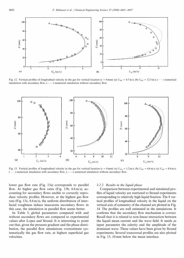
Fig. 12. Vertical pro"les of longitudinal velocity in the gas for vertical location (y"0mm): (a) UGS

"4.7m/s; (b) UGS

"12.5m/s; (**) numericalsimulation with secondary #ow, (- - - - -) numerical simulation without secondary #ow.

Fig. 13. Vertical pro"les of longitudinal velocity in the gas for vertical location (y"0mm): (a) UGS

"1.2 m/s; (b) UGS

"6.6 m/s; (c) UGS

"8.6 m/s;(**) numerical simulation with secondary #ow, (- - - - -) numerical simulation without secondary #ow.

lower gas #ow rate (Fig. 13a) corresponds to parallel#ow. At higher gas #ow rates (Fig. 13b, 6.6m/s), ac-counting for secondary #ows enable to correctly repro-duce velocity pro"les. However, at the highest gas #owrate (Fig. 13c, 8.6m/s), the uniform distribution of inter-facial roughness induce inaccurate secondary #ows: inthis case, the simulation in parallel #ow seems better.

In Table 5, global parameters computed with andwithout secondary #ows are compared to experimentalvalues after Lopez and Strand. It is interesting to pointout that, given the pressure gradient and the phase distri-bution, the parallel #ow simulations overestimate sys-tematically the gas #ow rate, at highest super"cial gasvelocities.

3.2.2. Results in the liquid phaseComparison between experimental and simulated pro-"les of liquid velocity are restricted to Strand experimentscorresponding to relatively high liquid fraction. The 8 ver-tical pro"les of longitudinal velocity in the liquid on thevertical axis of symmetry of the channel are plotted in Fig.14. The pro"les are well estimated in the simulations. Itcon"rms that the secondary #ow mechanism is correct.Recall that it is related to non-linear interaction betweenthe liquid mean current and the wave "eld. It needs asinput parameter the celerity and the amplitude of thedominant wave. These values have been given by Strandexperiments. Several transversal pro"les are also plottedin Fig. 15, 10 mm below the mean interface.


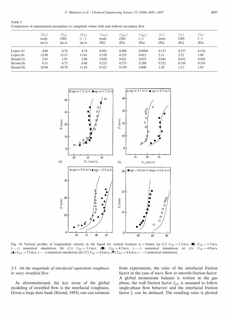
Table 5Comparison of experimental parameters to computed values with and without secondary #ow

SUgT SU

gT SU

gT Ss

wGT Ss

wGT Ss

pGT Ss

iT Ss

iT Ss

iT

(exp) (3D) (/ / ) (exp) (3D) (/ /) (exp) (3D) (/ /)(m/s) (m/s) (m/s) (Pa) (Pa) (Pa) (Pa) (Pa) (Pa)

Lopez (1) 4.88 4.76 4.74 0.091 0.090 0.0904 0.153 0.157 0.154Lopez (4) 12.80 13.15 13.61 0.528 0.525 0.612 2.11 2.22 1.69Strand (1) 2.03 1.91 2.06 0.020 0.021 0.023 0.041 0.032 0.028Strand (6) 8.31 8.75 8.80 0.232 0.273 0.280 0.552 0.536 0.510Strand (8) 10.08 10.70 11.16 0.321 0.350 0.400 1.20 1.12 1.03

Fig. 14. Vertical pro"les of longitudinal velocity in the liquid for vertical location (y"0mm): (a) (h) UGS

"1.2 m/s, (j) UGS

"1.7 m/s,(**) numerical simulation; (b) (L) U

GS"3.1 m/s, (v) U

GS"4.3 m/s, (**) numerical simulation; (c) (n) U

GS"4.9 m/s,

(m) UGS

"5.5m/s, (**) numerical simulation; (d) (£) UGS

"6.6 m/s, (.) UGS

"8.6 m/s, (**) numerical simulation.

3.3. On the magnitude of interfacial equivalent roughnessin wavy stratixed yow

As aforementioned, the key stone of the globalmodeling of strati"ed #ow is the interfacial roughness.Given a large data bank (Strand, 1993), one can estimate

from experiments, the ratio of the interfacial frictionfactor in the case of wavy #ow to smooth friction factor.A global momentum balance is written in the gasphase, the wall friction factor f

wGis assumed to follow

single-phase #ow behavior and the interfacial frictionfactor f

ican be deduced. The resulting ratio is plotted


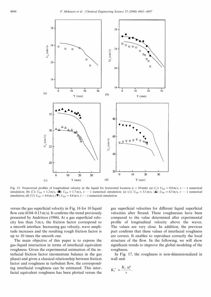
Fig. 15. Transversal pro"les of longitudinal velocity in the liquid for horizontal location (z"10 mm): (a) (L) UGS

"0.0m/s, (**) numericalsimulation; (b) (h) U

GS"1.2m/s, (j) U

GS"1.7 m/s, (**) numerical simulation; (c) (n) U

GS"3.1m/s, (m) U

GS"4.3 m/s, (**) numerical

simulation; (d) (£) UGS

"6.6m/s, (.) UGS

"8.6m/s, (**) numerical simulation.

versus the gas super"cial velocity in Fig. 16 for 10 liquid#ow rate (0.04}0.13m/s). It con"rms the trend previouslypresented by Andritsos (1986). At a gas super"cial velo-city less than 5m/s, the friction factor correspond toa smooth interface. Increasing gas velocity, wave ampli-tude increases and the resulting rough friction factor isup to 10 times the smooth one.

The main objective of this paper is to express thegas}liquid interaction in terms of interfacial equivalentroughness. Given the experimental estimation of the in-terfacial friction factor (momentum balance in the gasphase) and given a classical relationship between frictionfactor and roughness in turbulent #ow, the correspond-ing interfacial roughness can be estimated. This inter-facial equivalent roughness has been plotted versus the

gas super"cial velocities for di!erent liquid super"cialvelocities after Strand. These roughnesses have beencompared to the value determined after experimentalpro"le of longitudinal velocity above the waves.The values are very close. In addition, the previouspart con"rms that these values of interfacial roughnessare correct. It enables to reproduce correctly the localstructure of the #ow. In the following, we will showsigni"cant trends to improve the global modeling of theroughness.

In Fig. 17, the roughness is non-dimensionalized inwall unit

K`i"

Ki

uHi

l.


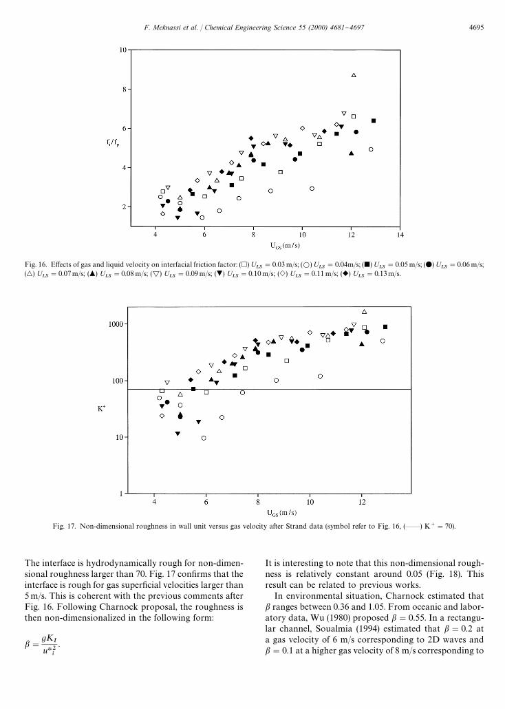
Fig. 16. E!ects of gas and liquid velocity on interfacial friction factor: (h) ULS

"0.03m/s; (L) ULS

"0.04m/s; (j) ULS

"0.05m/s; (v) ULS

"0.06m/s;(n) U

LS"0.07m/s; (m) U

LS"0.08 m/s; (£) U

LS"0.09m/s; (.) U

LS"0.10m/s; (e) U

LS"0.11 m/s; (r) U

LS"0.13m/s.

Fig. 17. Non-dimensional roughness in wall unit versus gas velocity after Strand data (symbol refer to Fig. 16, (**) K`"70).

The interface is hydrodynamically rough for non-dimen-sional roughness larger than 70. Fig. 17 con"rms that theinterface is rough for gas super"cial velocities larger than5m/s. This is coherent with the previous comments afterFig. 16. Following Charnock proposal, the roughness isthen non-dimensionalized in the following form:

b"gK

IuH2

i

.

It is interesting to note that this non-dimensional rough-ness is relatively constant around 0.05 (Fig. 18). Thisresult can be related to previous works.

In environmental situation, Charnock estimated thatb ranges between 0.36 and 1.05. From oceanic and labor-atory data, Wu (1980) proposed b"0.55. In a rectangu-lar channel, Soualmia (1994) estimated that b"0.2 ata gas velocity of 6 m/s corresponding to 2D waves andb"0.1 at a higher gas velocity of 8 m/s corresponding to


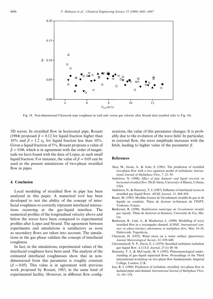
Fig. 18. Non-dimensional Charnock-type roughness in wall unit versus gas velocity after Strand data (symbol refer to Fig. 16).

3D waves. In strati"ed #ow in horizontal pipe, Rosant(1984) proposed b"0.12 for liquid fraction higher than10% and b"1.2 a

Lfor liquid fraction less than 10%.

Given a liquid fraction of 5%, Rosant proposes a value ofb"0.06, which is in agreement with the order of magni-tude we have found with the data of Lopez, at such smallliquid fraction. For instance, the value of b"0.05 can beused in the present simulations of two-phase strati"ed#ow in pipes.

4. Conclusion

Local modeling of strati"ed #ow in pipe has beenanalyzed in this paper. A numerical tool has beendeveloped to test the ability of the concept of inter-facial roughness to correctly represent interfacial interac-tions occurring at the gas}liquid interface. Thenumerical pro"les of the longitudinal velocity above andbelow the waves have been compared to experimentalpro"les after Lopez and Strand. The agreement betweenexperiments and simulations is satisfactory as soonas secondary #ows are taken into account. The simula-tions in the gas phase validate the concept of interfacialroughness.

In fact, in the simulations, experimental values of theinterfacial roughness have been used. The analysis of theestimated interfacial roughnesses show that in non-dimensional form this parameter is roughly constant(b"0.05). This value is in agreement with previouswork proposed by Rosant, 1983, in the same kind ofexperimental facility. However, in di!erent #ow con"g-

urations, the value of this parameter changes. It is prob-ably due to the evolution of the wave "eld. In particular,in external #ow, the wave amplitude increases with thefetch, leading to higher value of the parameter b.

References

Akai, M., Inoue, A., & Aoki, S. (1981). The prediction of strati"edtwo-phase #ow with a two equation model of turbulence. Interna-tional Journal of Multiphase Flow, 7, 21}39.

Andritsos, N. (1986). Ewect of pipe diameter and liquid viscosity onhorizontal stratixed yow. Ph.D. thesis, University of Illinois, Urbana,USA.

Andritsos, N., & Hanratty, T. J. (1987). In#uence of interfacial waves instrati"ed gas}liquid #ows. AIChE Journal, 33, 444}454.

Banat, M. (1985). Modeles locaux de l'eH coulement strati"eH de gaz et deliquide en conduite. These de docteur es-Sciences de l'INPT,Toulouse, France.

Benkirane, R. (1990). Mode& lisation nume& rique de l'e& coulement stratixe&gaz}liquide. These de doctorat es-Sciences, UniversiteH de Fes, Ma-roc.

Benkirane, R., LineH , A., & Masbernat, L. (1990). Modelling of wavystrati"ed #ow in a rectangular channel. ICHMT, International sem-inar on phase-interface phenomena in multiphase yow, May 14}18,Dubrovnik, Yugoslavia.

Charnock, H. (1955). Wind stress on a water surface. QuarternaryJournal Meteorological Society, 81, 639}640.

Cheremisino!, N. P., Davis, E. J. (1979). Strati"ed turbulent}turbulentgas}liquid #ow. A.I.Ch.E Journal, 25 (1) 48}56.

Hanratty, T. J., & McCready, M. J. (1992). Phenomenological under-standing of gas}liquid separated #ows. Proceedings of the Thirdinternational workshop on two-phase #ow fundamentals. ImperialCollege, London, U.K.

Issa, R. I. (1988). Prediction of turbulent, strati"ed, two-phase #ow ininclined pipes and channel. International Journal of Multiphase Flow,14, 141}154.


Jayanti, S., Wilke, N. S., Clarke, D. S., & Hewitt, G. F. (1989). Theprediction of turbulent yows over non gherred surfaces and its applica-tion to interpretation of mechanisms of horizontal annular yow.UKAEA report No AERE R 13697.

LineH , A., & Fabre, J. (1996). Strati"ed #ow, international encyclo-pedia of heat and mass transfer (pp. 1015}1021), Innodata Corpora-tion.

LineH , A., Masbernat, L., & Soualmia, A. (1996). Interfacial interactionand secondary #ows in strati"ed two-phase #ow. Chemical Engin-eering Communication 141}142, 303}329.

Lopez, D. (1994). Ecoulements diphasiques a% phases se&pare&es a% faiblecontenu de liquide. These de doctorat, I.N.P. Toulouse, France.

Magnaudet, J. (1989). Interactions interfaciales en e&coulement a% phasesse&pare&es. These de doctorat, INP Toulouse, France.

Rosant, J. M. (1983). Ecoulements diphasiques liquide-gaz enconduite circulaire. These de doctorat es-Sciences, ENSM, Nantes,France.

Shoham, O., & Taitel, Y. (1984). Strati"ed turbulent-turbulentgas}liquid #ow in horizontal and inclined pipes. AIChE Journal, 30,377}385.

Sinai, Y. L. (1985). Interfacial phenomena of fully-developed, strati"ed,two-phase #ows. In: N. P. Cheremisino! (Ed.), Encyclopedia of -uidmechanics, gas}liquid -ows, vol. 3, (pp. 475}491) Houston: GulfPublishing Co.

Soualmia, A. (1993). Analyse physique et mode& lisation des e&coulementsgaz}liquide a% phases se&pare&es. These de doctorat de l'INPT,Toulouse, France.

Strand, O. (1993). An experimental investigation of stratixed two-phaseyow in horizontal pipes. Ph.D. thesis, Univ. of Oslo, Norway.

Suzanne, C. (1985). Structure de l'eH coulement strati"eH de gaz et deliquide en canal rectangulaire. These de docteur es-Sciences del'INPT, Toulouse, France.

Taitel, Y., & Dukler, A. E. (1976a). A theoretical approach to theLockhart}Martinelli correlation for strati"ed #ow. InternationalJournal of Multiphase Flow, 2, 591}595.

Taitel, Y., & Dukler, A. E. (1976b). Model for predicting #ow regimetransitions in horizontal and near horizontal gas}liquid #ow. AIChEJournal, 22, 47}55.

Wu, J. (1980). Wind stress coe$cients over sea surface near neutralconditions. American Meteorological Society, 10, 727}740.


Numerical modeling of wavy stratified two-phase flow in pipes

Documents