Discrete Fourier Transform Part: Discrete Fourier Transform http://numericalmethods.eng.usf. edu

Numerical Methods Discrete Fourier Transform Part: Discrete Fourier Transform .
Dec 25, 2015
Welcome message from author
This document is posted to help you gain knowledge. Please leave a comment to let me know what you think about it! Share it to your friends and learn new things together.
Transcript

Numerical Methods
Discrete Fourier Transform Part: Discrete Fourier Transform
http://numericalmethods.eng.usf.edu

For more details on this topic
Go to http://numericalmethods.eng.usf.edu
Click on Keyword Click on Discrete Fourier Transform
You are free
to Share – to copy, distribute, display and perform the work
to Remix – to make derivative works

Under the following conditions Attribution — You must attribute the
work in the manner specified by the author or licensor (but not in any way that suggests that they endorse you or your use of the work).
Noncommercial — You may not use this work for commercial purposes.
Share Alike — If you alter, transform, or build upon this work, you may distribute the resulting work only under the same or similar license to this one.
Chapter 11.04 : Discrete Fourier Transform (DFT)
Major: All Engineering Majors
Authors: Duc Nguyen
http://numericalmethods.eng.usf.edu
Numerical Methods for STEM undergraduates04/19/23
http://numericalmethods.eng.usf.edu 5
Lecture # 8
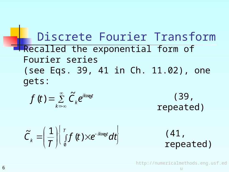
Discrete Fourier TransformRecalled the exponential form of Fourier series (see Eqs. 39, 41 in Ch. 11.02), one gets:
k
tikw
keCtf 0~)(
Ttikw
k dtetfT
C0
0)(1~
(39, repeated)
(41, repeated)
http://numericalmethods.eng.usf.edu6

http://numericalmethods.eng.usf.edu7
,,.......,3,2, 321 tnttttttt n
then Eq. (39) becomes:
1
0
0~)(
N
k
ntikw
kn eCtf (1)
If time “ ” is discretized at t
Discrete Fourier Transform
Discrete Fourier Transform cont.
To simplify the notation, define:
ntn (2)
Then, Eq. (1) can be written as:
1
0
0~)(
N
k
nikw
keCnf (3)
Multiplying both sides of Eq. (3) by nilwe 0
, and performing
the summation on “ ”, onen obtains (note: l = integernumber)
http://numericalmethods.eng.usf.edu8
http://numericalmethods.eng.usf.edu9
nilwN
n
N
k
nikw
k
N
n
nilw eeCenf 01
0
1
0
01
0
0 ~)(
1
0
1
0
2)(~N
n
N
k
nN
lki
keC
(4)
(5)
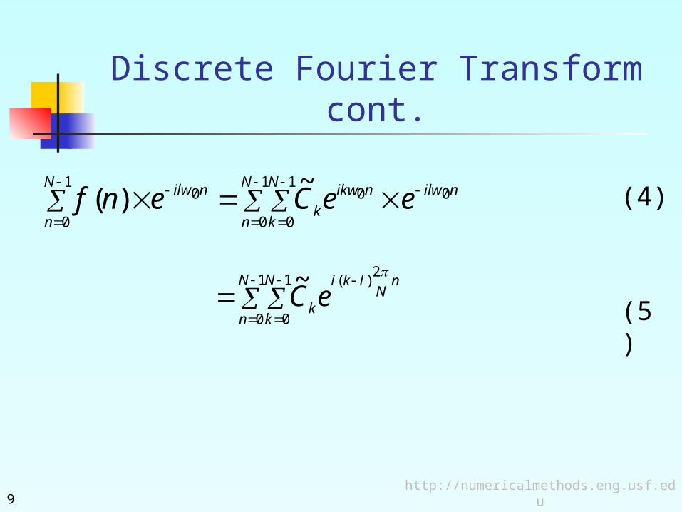
Discrete Fourier Transform cont.
Discrete Fourier Transform cont.
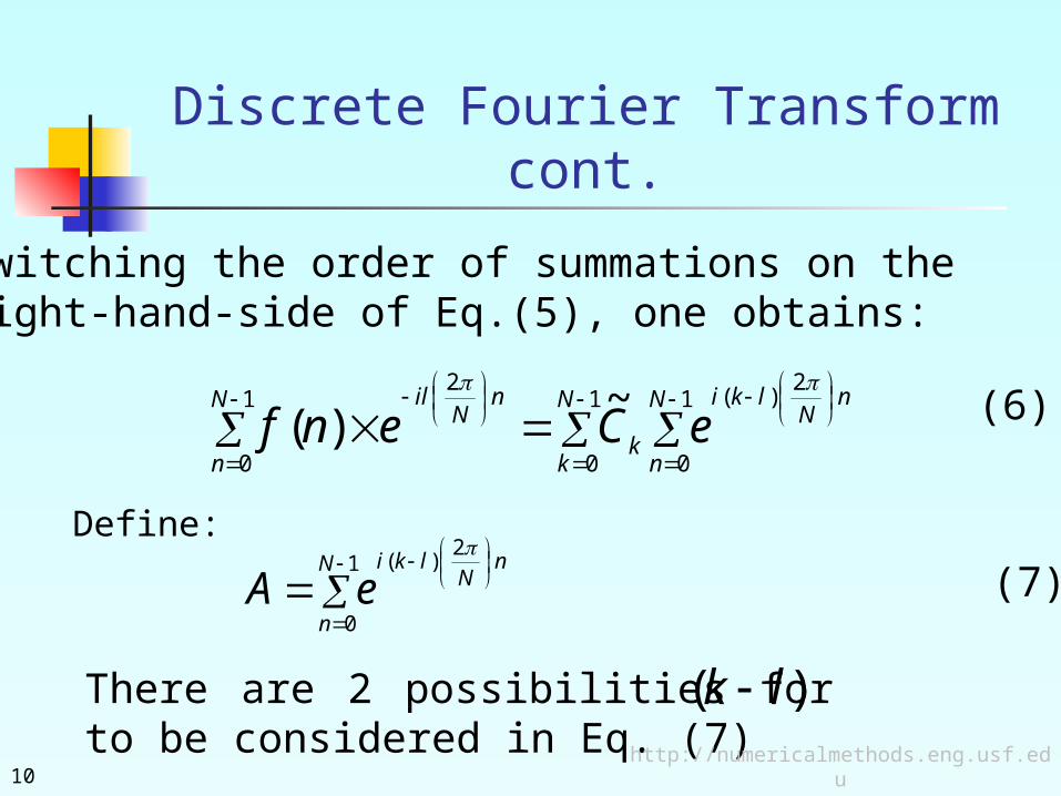
Switching the order of summations on the right-hand-side of Eq.(5), one obtains:
1
0
1
0
2)(1
0
2 ~)(
N
k
N
n
nN
lki
k
N
n
nN
il
eCenf
(6)
Define:
1
0
2)(N
n
nN
lki
eA
(7)
There are 2 possibilities for to be considered in Eq. (7)
)( lk
http://numericalmethods.eng.usf.edu10

Discrete Fourier Transform—Case 1
Case(1): is a multiple integer of N, such as: ; or where
)( lk mNlk )( mNlk
,......2,1,0 m
Thus, Eq. (7) becomes:
1
0
1
0
2 )2sin()2cos(N
n
N
n
nim mnimneA (8)
Hence:
(9)NA
http://numericalmethods.eng.usf.edu11
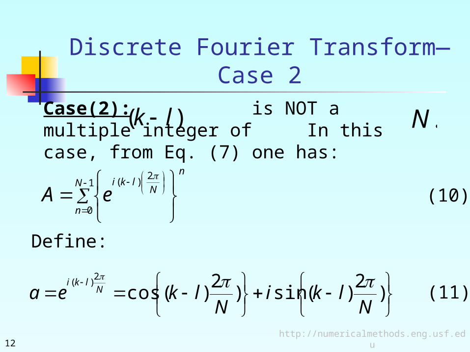
Discrete Fourier Transform—Case 2
Case(2): is NOT a multiple integer of In this case, from Eq. (7) one has:
)( lk .N
1
0
2)(N
n
n
Nlki
eA
(10)
Define:
)
2)(sin)
2)(cos
2)(
Nlki
Nlkea N
lki
(11)
http://numericalmethods.eng.usf.edu12

http://numericalmethods.eng.usf.edu13
;1a because is “NOT” a multiple integer of )( lk NThen, Eq. (10) can be expressed as:
1
0
N
n
naA (12)
Discrete Fourier Transform—Case 2

Discrete Fourier Transform—Case 2
From mathematical handbooks, the right side of Eq. (12) represents the “geometric series”, and can be expressed as:
;1
0NaA
N
n
n
if 1a (13)
;1
1
a
aN
if 1a (14)
http://numericalmethods.eng.usf.edu14

http://numericalmethods.eng.usf.edu15
Because of Eq. (11), hence Eq. (14) should be usedto compute . Thus:A
a
e
a
aA
lkiN
1
1
1
1 2)(
(See Eq. (10)) (15)
12)(sin2)(cos2)( lkilke lki (16)
Discrete Fourier Transform—Case 2
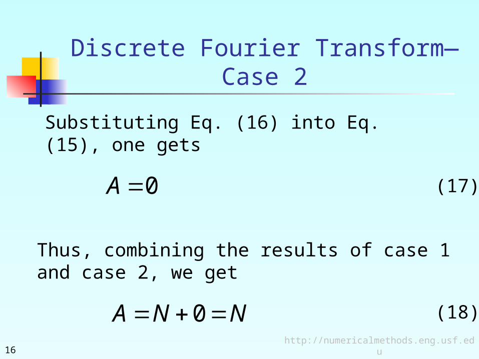
Discrete Fourier Transform—Case 2
Substituting Eq. (16) into Eq. (15), one gets
0A (17)
Thus, combining the results of case 1 and case 2, we get
NNA 0 (18)
http://numericalmethods.eng.usf.edu16

THE ENDhttp://numericalmethods.eng.usf.edu

This instructional power point brought to you byNumerical Methods for STEM undergraduatehttp://numericalmethods.eng.usf.eduCommitted to bringing numerical methods to the undergraduate
Acknowledgement

For instructional videos on other topics, go to
http://numericalmethods.eng.usf.edu/videos/
This material is based upon work supported by the National Science Foundation under Grant # 0717624. Any opinions, findings, and conclusions or recommendations expressed in this material are those of the author(s) and do not necessarily reflect the views of the National Science Foundation.

The End - Really
Numerical Methods
Discrete Fourier Transform Part: Discrete Fourier Transform
http://numericalmethods.eng.usf.edu

For more details on this topic
Go to http://numericalmethods.eng.usf.edu
Click on Keyword Click on Discrete Fourier Transform

You are free
to Share – to copy, distribute, display and perform the work
to Remix – to make derivative works

Under the following conditions Attribution — You must attribute the
work in the manner specified by the author or licensor (but not in any way that suggests that they endorse you or your use of the work).
Noncommercial — You may not use this work for commercial purposes.
Share Alike — If you alter, transform, or build upon this work, you may distribute the resulting work only under the same or similar license to this one.
http://numericalmethods.eng.usf.edu25
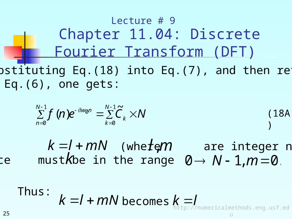
Substituting Eq.(18) into Eq.(7), and then referring to Eq.(6), one gets:
1
0
1
0
0 ~)(
N
kk
N
n
nilw NCenf (18A)
Recall (where are integer numbers), And since must be in the range
mNlk ml,k .0,10 mN
mNlk lk becomes
Chapter 11.04: Discrete Fourier Transform (DFT)
Lecture # 9
Thus:
Discrete Fourier Transform—Case 2
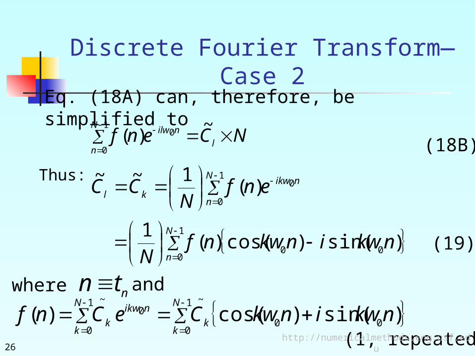
Eq. (18A) can, therefore, be simplified to
NCenf l
N
n
nilw
~)(
1
0
0
(18B)
Thus:
1
000
1
0
0
)sin()cos()(1
)(1~~
N
n
N
n
nikw
kl
nkwinkwnfN
enfN
CC
(19)
where ntn and
1
000
~1
0
0~
)sin()cos()(N
kk
N
k
nikw
k nkwinkwCeCnf(1, repeated)
http://numericalmethods.eng.usf.edu26

Discrete Fourier Transform cont.
Equations (19) and (1) can be rewritten as
1
0
20
)(~ N
k
nN
wik
n ekfC
(20)
1
0
20~1
)(N
n
nN
wik
neCNkf
(21)
http://numericalmethods.eng.usf.edu27
http://numericalmethods.eng.usf.edu28
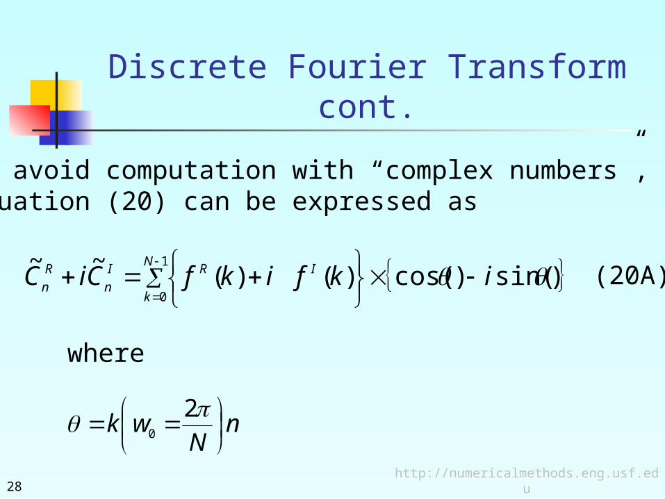
To avoid computation with “complex numbers”, Equation (20) can be expressed as
1
0)sin()cos()()(
~~ N
k
IRI
n
R
n ikfikfCiC (20A)
where
nN
wk
2
0
Discrete Fourier Transform cont.
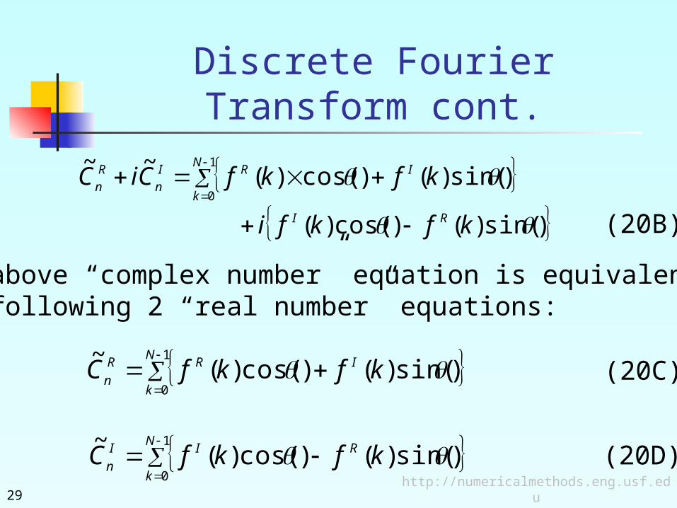
Discrete Fourier Transform cont.
)sin()()cos()(
)sin()()cos()(~~ 1
0
kfkfi
kfkfCiC
RI
N
k
IRI
n
R
n
(20B)
The above “complex number” equation is equivalent to the following 2 “real number” equations:
1
0)sin()()cos()(
~ N
k
IRR
n kfkfC
1
0)sin()()cos()(
~ N
k
RII
n kfkfC
(20C)
(20D)
http://numericalmethods.eng.usf.edu29

THE ENDhttp://numericalmethods.eng.usf.edu
This instructional power point brought to you byNumerical Methods for STEM undergraduatehttp://numericalmethods.eng.usf.eduCommitted to bringing numerical methods to the undergraduate
Acknowledgement

For instructional videos on other topics, go to
http://numericalmethods.eng.usf.edu/videos/
This material is based upon work supported by the National Science Foundation under Grant # 0717624. Any opinions, findings, and conclusions or recommendations expressed in this material are those of the author(s) and do not necessarily reflect the views of the National Science Foundation.

The End - Really
Numerical Methods
Discrete Fourier Transform Part: Aliasing Phenomenon Nyquist Samples, Nyquist rate
http://numericalmethods.eng.usf.edu

For more details on this topic
Go to http://numericalmethods.eng.usf.edu
Click on Keyword Click on Discrete Fourier Transform

You are free
to Share – to copy, distribute, display and perform the work
to Remix – to make derivative works

Under the following conditions Attribution — You must attribute the
work in the manner specified by the author or licensor (but not in any way that suggests that they endorse you or your use of the work).
Noncommercial — You may not use this work for commercial purposes.
Share Alike — If you alter, transform, or build upon this work, you may distribute the resulting work only under the same or similar license to this one.

Chapter 11.04: Aliasing Phenomenon, Nyquist samples,
Nyquist rate (Contd.)When a function ),(tf which may represent the signals from some real-life phenomenon (shown in Figure 1), is sampled, it basically converts that function into a sequence )(
~kf at discrete locations of .t
http://numericalmethods.eng.usf.edu38
Lecture # 10
Figure 1: Function to be sampled and “Aliased” sample problem.
Aliasing Phenomenon, Nyquist samples, Nyquist rate cont.
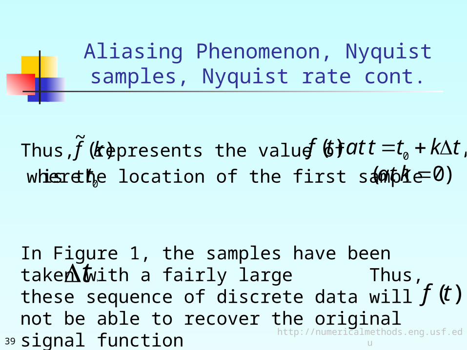
)(~kf ,)( 0 tkttattf represents the value of Thus,
where 0tis the location of the first sample ).0( kat
In Figure 1, the samples have been taken with a fairly large Thus, these sequence of discrete data will not be able to recover the original signal function
.t).(tf
http://numericalmethods.eng.usf.edu39
Aliasing Phenomenon, Nyquist samples, Nyquist rate cont.
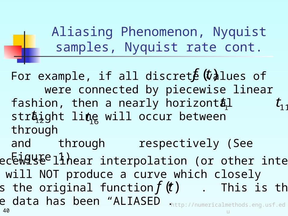
These piecewise linear interpolation (or other interpolationschemes) will NOT produce a curve which closely resembles the original function . This is the case where the data has been “ALIASED”.
)(tf
http://numericalmethods.eng.usf.edu40
For example, if all discrete values of were connected by piecewise linear fashion, then a nearly horizontal straight line will occur between through and through respectively (See Figure 1).
)(tf
1t 11t16t12t
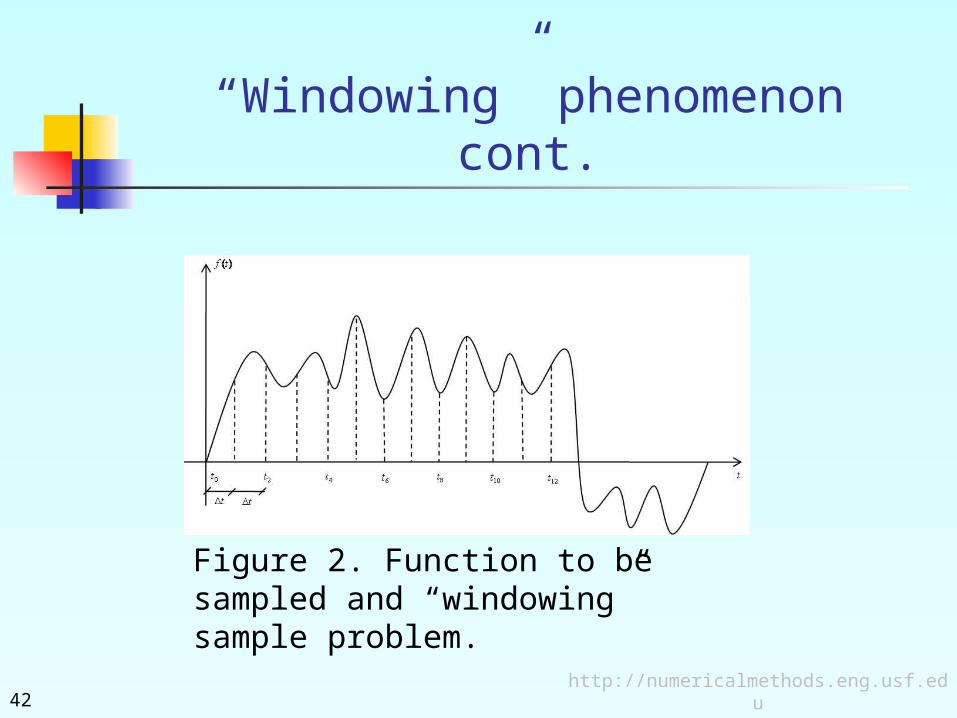
“Windowing” phenomenon
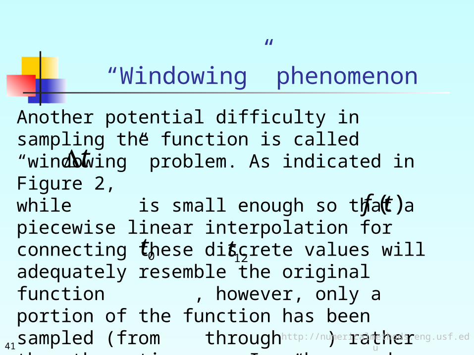
Another potential difficulty in sampling the function is called “windowing” problem. As indicated in Figure 2, while is small enough so that a piecewise linear interpolation for connecting these discrete values will adequately resemble the original function , however, only a portion of the function has been sampled (from through ) rather than the entire one. In other words, one has placed a “window” over the function.
t
)(tf
0t 12t
http://numericalmethods.eng.usf.edu41
“Windowing” phenomenon cont.
Figure 2. Function to be sampled and “windowing” sample problem.
http://numericalmethods.eng.usf.edu42

“Nyquist samples, Nyquist rate”
Figure 3. Frequency of sampling rate versus maximum frequency content
)( Sw ).( maxw
In order to satisfy the frequency ( ) should be between points A and B of Figure 3.
max0)( wwforwF w
http://numericalmethods.eng.usf.edu43

Hence:
maxmax wwww s
which implies:
max2wws
Physically, the above equation states that one must have at least 2 samples per cycle of the highest frequency component present (Nyquist samples, Nyquist rate).
http://numericalmethods.eng.usf.edu44
“Nyquist samples, Nyquist rate”
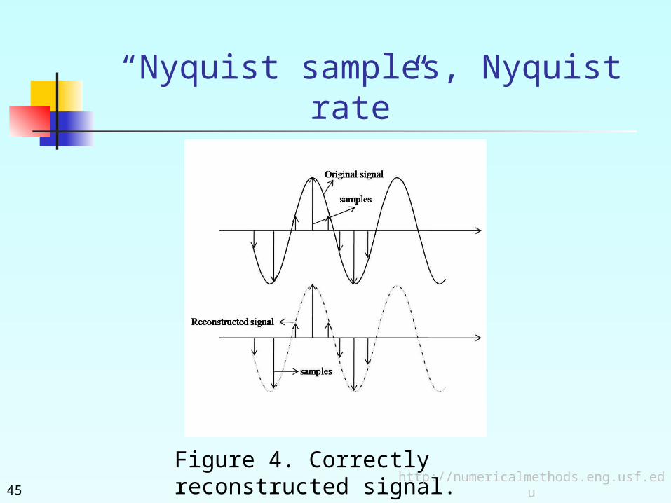
Figure 4. Correctly reconstructed signal.
http://numericalmethods.eng.usf.edu45
“Nyquist samples, Nyquist rate”

In Figure 4, a sinusoidal signal is sampled at the rate of 6 samples per 1 cycle (or ). Since this sampling rate does satisfy the sampling theorem requirement of , the reconstructed signal does correctly represent the original signal.
06wws
max2wws
http://numericalmethods.eng.usf.edu46
“Nyquist samples, Nyquist rate”

Figure 5. Wrongly reconstructed signal.
In Figure 5 a sinusoidal signal is sampled at the rate of 6 samples per 4 cycles
04
6wwor s
Since this sampling rate does NOT satisfy the requirement the reconstructed signal was wrongly represent the original signal!
,2 maxwws
http://numericalmethods.eng.usf.edu47
“Nyquist samples, Nyquist rate”

THE ENDhttp://numericalmethods.eng.usf.edu

This instructional power point brought to you byNumerical Methods for STEM undergraduatehttp://numericalmethods.eng.usf.eduCommitted to bringing numerical methods to the undergraduate
Acknowledgement

For instructional videos on other topics, go to
http://numericalmethods.eng.usf.edu/videos/
This material is based upon work supported by the National Science Foundation under Grant # 0717624. Any opinions, findings, and conclusions or recommendations expressed in this material are those of the author(s) and do not necessarily reflect the views of the National Science Foundation.

The End - Really
Related Documents