DISCRETE FOURIER TRANSFORM 1. Introduction The sampled discrete-time fourier transform (DTFT) of a finite length, discrete-time signal is known as the discrete Fourier transform (DFT). The DFT contains a finite number of samples equal to the number of samples N in the given signal. Computationally efficient algorithms for implementing the DFT go by the generic name of fast Fourier transforms (FFTs). This chapter describes the DFT and its properties, and its relationship to DTFT. 2. Definition of DFT and its Inverse Lest us consider a discrete time signal x (n) having a finite duration, say in the range 0 ≤ n ≤N-1. The DTFT of the signal is N-1 X ( ω) = Σ x (n)e -jwn (1) n-0 Let us sample X using a total of N equally spaced samples in the range : ω ∈(0,2π), so the sampling interval is 2π That is, we sample X(ω) using the frequencies. N ω= ωk = 2π k , 0 ≤ k ≤N-1. N-1 Thus X (k) = Σ x (n)e -jwn (2) n-0 N-1 X (k) = Σ x (n)e - j2π kn (2) n-0 N The result is, by definition the DFT. That is , Equation (0.2) is known as N-point DFT analysis equation. Fig 0.1 shows the Fourier transform of a discrete – time signal and its DFT samples.

Welcome message from author
This document is posted to help you gain knowledge. Please leave a comment to let me know what you think about it! Share it to your friends and learn new things together.
Transcript

DISCRETE FOURIER TRANSFORM
1. Introduction
The sampled discrete-time fourier transform (DTFT) of a finite length, discrete-time signal is
known as the discrete Fourier transform (DFT). The DFT contains a finite number of samples
equal to the number of samples N in the given signal. Computationally efficient algorithms for
implementing the DFT go by the generic name of fast Fourier transforms (FFTs). This chapter
describes the DFT and its properties, and its relationship to DTFT.
2. Definition of DFT and its Inverse
Lest us consider a discrete time signal x (n) having a finite duration, say in the range 0 ≤ n ≤N-1.
The DTFT of the signal is
N-1
X ( ω) = Σ x (n)e-jwn (1)
n-0
Let us sample X using a total of N equally spaced samples in the range : ω ∈(0,2π), so the
sampling interval is 2π That is, we sample X(ω) using the frequencies.
N
ω= ωk = 2πk , 0 ≤ k ≤N-1. N-1
Thus X (k) = Σ x (n)e-jwn (2)
n-0
N-1
X (k) = Σ x (n)e-
j2πkn (2)
n-0
N
The result is, by definition the DFT.
That is ,
Equation (0.2) is known as N-point DFT analysis equation. Fig 0.1 shows the Fourier transform
of a discrete – time signal and its DFT samples.

x(w)
0 π 2π →w
Fig.1 Sampling of X(w) to get x(k)
While working with DFT, it is customary to introduce a complex quantity
WN = e-j2π /N
Also, it is very common to represent the DFT operation
N=1
X(k) = DFT ( x(n)) = Σ x(n) WNkn, 0≤n≤N-1
n=0
The complex quantity Wn is periodic with a period equal to N. That is,
WNa+N = e-j+2π/N(a+N) = e-j2π /N n = WN
a where a is any integer.
Figs. 0.2(a) and (b) shows the sequence for 0≤n≤N-1 in the z-plane for N being even and
odd respectively.
6 5
5 7 4 6
4 0 0
3 1 3 1
2 2
(a) (b)
Fig.2 The Sequence for even N (b) The sequence for odd N.
The sequence WkN
N for 0 ≤ n ≤ N-1 lies on a circle of unit radius in the complex plane
and the phases are equally spaced, beginning at zero.
The formula given in the lemma to follow is a useful tool in deriving and analyzing
various DFT oriented results.

2.1. Lemma
N-1
Σ Wkn = N δ (k) = { N, k = 0 (3)
n-0 N 0, k ≠ 0
Proof :
N-1
Σ an
= 1 - aN
: a≠ 1
n-0 1 - a
We know that
Applying the above result to the left side of equation (3.3), we get
N-1
Σ (WkN) n = 1- Wk
NN = 1- e-j2π kN
N
n= 0 1- Wk
NN 1- e-j2π k
NN : k ≠ 0
= 1 - 1
1- e- j2π kN
N
= 0, k ≠ 0
when k = 0, the left side of equation (3.3) becomes
N-1 N-1
Σ WN0xn = Σ 1 = N
n= 0 n =0
N-1 N, k = 0
Hence, we may write Σ WN
0xn = 0, k ≠ 0
n=0
= N δ (k), 0≤ k≤ N-1
2.2 Inverse DFT
The DFT values (X(k), 0≤ k≤ N-1), uniquely define the sequence x(n) through the inverse DFT
formula (IDFT) :
N-1
x (n) = IDFT (X(k) = 1 Σ X(k) WN-kn , 0≤ k≤ N-1
N k=0
The above equation is known as the synthesis equation.

N-1 N-1 N-1
Proof : 1 Σ X(k) WN-kn = 1 Σ [Σ x(m) WN
km] = WN-kn
N k=0 N k=0 m=0
N-1 N-1 N-1
= 1 Σ x(m) [Σ WN
-(n-m)k]
N k=0 m=0
It can be shown that
N-1
Σ WN(n-m)k = N , n = m
0, n ≠ m
Hence,
N-1
1 Σ x(m) Nδ (n-m)
N
= 1 x Nx (m) ( sifting property)
N m=n
= x(n)
2.3 Periodicity of X (k) and x (n)
The N-point DFT and N-point IDFT are implicit period N. Even though x (n) and X (k) are
sequences of length – N each, they can be shown to be periodic with a period N because the
exponentials WN±kn in the defining equations of DFT and IDFT are periodic with a period N. For
this reason, x (n) and X (k) are called implicit periodic sequences. We reiterate the fact that for
finite length sequences in DFT and IDFT analysis periodicity means implicit periodicity. This
can be proved as follows :
N-1
X (k) = Σ x(n) WNkn
N-p=0
⇒ X (k+N) = Σ x(n) WN(k+N)n
Since, WNNn = e-j2πnNn = 1, we get
N-1
X (k+N) = Σ x(n) WN-kn
n=0
= X (k)

N-1
Similarly, x (n) Σ X (k) WN-kn
k=0
N-1
⇒ x (n+N) = 1 Σ X(k) WN-k(n+N)
N k=0
N-1
= 1 Σ X(k) WN-kn WN
-kn
N k=0
Since, WN-kn = e-j2π/N kN = e-j2πk = 1, we get
N-1
x(n+N) = 1 Σ X(k) WN-kn
= x (n)
Since, DFT and its inverse are both periodic with period N, it is sufficient to compute the
results for one period (0 to N-1). We want to emphasize that both x (n) and X (k) have a starting
index of zero.
A very important implication of x (n), being periodic is, if we wish to find DFT of a
periodic signal, we extract one period of the periodic signal and then compute its DFT.
Example 1 Compute the 8 – point DFt of the sequence x (n) given below :
x (n) = (1,1,1,1,0,0,0,0)
Solution
The complex basis functions, W for 0 n 7 lie on a circle of unit radius as shown in Fig. Ex.3
W86
W85 W87
W84 1.0 Re(z)
W83 W81
W82
Fig. 3 Sequence W8
0 for 0≤ n ≤ 8.
Since N = 8 we get W = e –j2π/8
Thus,
W80 = 1
W81 = e -jπ/4 = 1 – j 1
√2 √2
W82 = e -jπ/2 = – j
W83 = e -j3π/4 = 1 – j 1
√2 √2
W84 = -W8
0 = -1
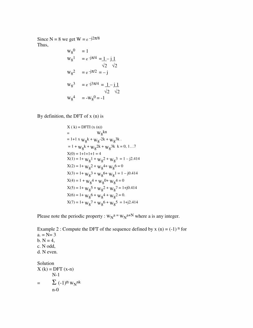
By definition, the DFT of x (n) is
X ( k) = DFTI (x (n))
= W8kn
= 1+1 x W8k + W8
-2k + W83k .
= 1 + W8k + W8
2k + W83k k = 0, 1…7
X(0) = 1+1+1+1 = 4
X(1) = 1+ W81 + W8
2 + W83 = 1 – j2.414
X(2) = 1+ W82 + W8
4+ W86 = 0
X(3) = 1+ W83 + W8
6+ W81 = 1 – j0.414
X(4) = 1 + W84 + W8
0+ W84 = 0
X(5) = 1+ W85 + W8
2 + W87 = 1+j0.414
X(6) = 1+ W86 + W8
4 + W82 = 0.
X(7) = 1+ W87 + W8
6 + W85 = 1+j2.414
Please note the periodic property : WNa = WN
a+N where a is any integer.
Example 2 : Compute the DFT of the sequence defined by x (n) = (-1) n for
a. = N= 3
b. N = 4,
c. N odd,
d. N even.
Solution
X (k) = DFT (x-n)
N-1
= Σ (-1)n WNnk
n-0

N-1
Σ (-1)n [WNk] n
n=0
= 1 – (1)N for WNk ≠-1
1+ WNk
a. N = 3
X(k) = 2 = 2 0≤ k ≤ 2
1+ WNk 1+ cos (2kπ/3) – j sin ((2πk/3)
b. N = 4 X (k) = 0 for W4k ≠-1 or k≠ 2
With k = 2 we get
N-1
X(2) Σ (-1)n W42n
n=0
= 1 - W42 + W4
4 - W46
= 1 – (-1) + (-1)2– (-1)2 = 4
Hence, X (k) = 48(k-2)
c. We know that
W42n – e-j2π / N k
If N = 2k, we get WNk= -1.
Since N is odd no k exists. This means to say that WNk ≠ -1 for all k from 0 to N-1.
Therefore,
X(k) = 2 0≤ k ≤ N-1
1+ WNk
d. N even WNk = - 1, if k = N/2.
X ( k) = 0 for k ≠ N/2
With k = 2, we get
N-1
And x (N/2) = Σ [- WNk] n
n=0
N-1
=Σ [1] = N
n=0
Hence X (k) = N δ (k-N/2)

Example 3. Compute the inverse DFT of the sequence,
X(k) = (2,1+j,0,1 –j)
Solution
x (n) = IDFT (X(k))
N-1
∆ 1 Σ x(n) WN-kn , 0 ≤ n ≤N -1
N n=0
Please note that :
WN-kn = [ WN
kn]*
Since, N = 4, we get
N-1
x (n) = 1 Σ X(k) W4-kn , 0 ≤ n ≤3
4 n=0
= 1 [X(0) W4-0xn + X(1) W4
-n + X (2) W4-2n + X (3) W4
-3n]
4
= 1 [2 + (1+j) W4-n +0 + (1-j) + X (3) W4
-3n]
4
Hence, x (0) = 1 [2 + (1+j) +(1-j)] = 1
4
x (1) = 1 [2 + (1+j) W4-1 +(1-j) W4
-3] = 1
4
x (2) = 1 [2 + (1+j) W4-2 +(1-j) W4
-6] = 1
4
Because of periodicity, W4-6 = W4
-2
Hence, x (2) = 1 [2 + (1+j) (-1) + (1-j) (-1)] = 0
4
x (3) = 1 [2 + (1+j) W4-3 +(1-j) W4
-9] = 1
4
Because of periodicity, W4-9 = W4
-5 = W4-1

Hence, x (3) = 1 [2 + (1+j) W4-3 +(1-j) W4
-1]
4
= 1 [2 + (1+j) (-j) (-j) + (1-j) ] = 1
4
Hence, x(n) = (1,0,0,1)
3. Matrix Relation for Computing DFT
The defining relation for DFT of a finite length sequence x (n) is
N-1
X (k) = Σ x(n) Wnkn , 0.1, …… N-1
n=0
Let us evaluate X (k) for different values of k in the range (0, N-1) as given below :
X (0) = WN0 x (0) + WN
0 x (1) + …… + WN0 x (N-1)
X (1) = WN0 x (0) + WN
1 x (1) + …… + WN(N-1) x (N-1)
X (2) = WN0 x (0) + WN
2 x (1) + …… + WN2(N-1) x (N-1)
X (N-1) = WN0 x (0) + WN
(N-1)x (1) + ….. =+ WN(N-1) (N-1) x (N-1)
Putting the N DFT equations in N unknowns in the matrix form, we get
X = WNx
Here X and x are (N x 1) matrices, and Wn is an (N x N) square matrix called the DFT matrix.
The full matrix form is described by
X(0) WN0 WN
0 WN0 … WN
0 x(0)
X(1) WN0 WN
1 WN2 … WN
(N-1) x(1)
X(2) = WN0 WN
2 WN4 … WN
kn x(2)
: : : : : :
X(N-1) WN0 WN
N-1 WN2(N-1)… WN
(N-1)(N-1) x(N-1)
The elements WNkn of WN are called complex basis functions or twiddle factors.
Example : Compute the 4-point DFT of the sequence, x(n) = (1,2,1,0).
Solution
With N = 4, W4 = e-j2 π /4 = -j.
We know that

X = WN x
X(0) W40 W4
0 W40 W4
0 x(0)
X(1) W40 W4
1 W42 W4
3 x(1)
X(2) = W40 W4
2 W44 W4
6 x(2)
X(3) W40 W4
3 W46 W4
0 x(3)
Exploiting the periodic property WN0 = WN
n+N where a is any integer the above matrix relation
becomes.
X(0) W40 W4
0 W40 W4
0 x(0)
X(1) W40 W4
1 W42 W43 x(1)
X(2) = W40 W4
2 W40 W4
2 x(2)
X(3) W40 W4
3 W42 W4
1 x(3)
X(0) 1 1 1 1 1
X(1) 1 -j -1 j 2
X(2) = 1 -1 1 -1 1
X(3) 1 j -1 -j 0
Hence,
X(k) = (4, -j2, 0, j2)
4. Matrix Relation for Computing IDFT
We know that x = WN1X
Premultiplying both the sides of the above equation by we get
WN-1-X = WN
-1 WNx
WN-1X = x
Or x = WN-1X
In the above equation (.8) x = WN-1 is called IDFT matrix.
The defining equation for finding IDFT of a sequence X (k) is

N-1
X (n) = 1 Σ X(k) W , 0≤ n ≤ N-1
N k=0
N-1
= 1 X Σ (k) [WNkn ]*
N k=0
The first set of N IDFT equation in N unknowns may be expressed in the matrix form as
x = 1 W*NX
N
Where W*N denotes the complex conjugate of WN. Comparision of equation (3.8) and (3.9)
leads us to conclude that
WN-1 = 1/N W*N
This very important result shows that W-1N requires only conjugation of Wn multiplied by 1/N.
an obvious computational advantage. The matrix relations (.7) and (.9) together define DFT as a
linear transformation.
5. Using the DFT to Find the IDFT
We know that
N-1
x* (n) = 1 Σ X(k) WN-kn , n= 0,1 …. N-1
N k=0
Taking complex conjugates on both the sides of the above equation, we get
N-1
x*(n) = 1 Σ X(k) WN-kn *
N k=0

N-1
⇒ x*(n) = 1 Σ X*(k) WN-kn * (10)
N k =0
The right – hand side of equation (3.10) is recognized as the DFT of X* (k), so we can rewrite
equation (3.10) as follows :
x*(n) = 1 DFT (X*(k))
N
Taking complex conjugates on both the sides of equation (11), we get
x*(n) = 1 [DFT (X*(k))]
N
The above results suggests the DFT algorithm itself can be used to find IDFT. In practice, this is
indeed what is done.
6. Properties of DFT
In the following section, we shall discuss some of the important properties of the DFt. They are
strikingly similar to other frequency domain transforms, but must always be used in keeping with
implied periodicity for both DFT and IDFT in time and frequency domains.
6.1 Linearity
DFT (ax1(n) + bx2(n)j = aX1(k) + bX2(k), k = 0, N =1
If X1(k) and X2(k) are the DFTs of the sequence x1 (n) and x2 (n), respectively, both of lengths
N.
Proof :
N-1
We know that DFT [x(n)] = Σ x(n) WNkn
n=0
Letting x (n) = ax1(n) + bx2(n) we get
N-1
DFT = ax1(n) + bx2(n) = Σ (ax1(n) +bx2 (n)] WNkn
n=0
N-1
= a Σ x1(n) WNkn + b Σ x1(n) WN
kn
n=0

= aX1 (k) + bX2(k), 0 ≤ k≤ N-1
Sometimes we represent the linearity property as given below
DFT
ax1 (n) + bx2(n) aX1 (k) + bX2(k)
Example : Find the 4- point DFT of the sequence
X(n) = cos ( π n) + sin ( π n)
4 4
Use linearity property.
Solution
Given N = 4,
WN = e j2π /n ⇒ W = e jπ /2
We know that, W40 = 1
Hence, W40 = 1
W41 = e = -j
W43 = e = -1
x1 (n) = cos (π /4 n )
Let
x2 (n) = sin (π /4 n )
and
Then, the values of x (n) and x2 (n) for 0 <n <3 tabulated below :
N x1 (n) = cos (π /4 n ) x2 (n) = sin (π /4 n )
0 1 0
1 1 1
√2 √2
2 0 1
3 -1 1
√2 √2
X1 (k) = DFT (x1 (n))
3
∆ Σ x1 (n) W4kn, k = 0,1,2,3
n=0
⇒ X1 (k) = 1 + 1 W4k +0 – 1 W4
3k

√2 √2
Hence, X1 (0) = 1 + 1 – 1 = 1
√2 √2
X1 (1) = 1 + 1 W41 – 1 W4
3 = 1 –j1.414
√2 √2
X1 (2) = 1 + 1 W42 – 1 W4
6
√2 √2
= 1 + 1 W42 – 1 W2
4 = 1
√2 √2
X1 (3) = 1 + 1 W43 – 1 W4
9
√2 √2
= 1 + 1 W43 – 1 W4
1
√2 √2
Similarly, X2 (k) = DFT (x2 (n))
3
∆ Σ x2 (n) W4kn
n=0 ⇒ X2 (k) = 1 W4
k + W42k + 1 W4
3k
√2 √2
Hence, X2 (0) = 1 + 1 + 1 = 2.414
√2 √2
X2 (1) = 1 W41 + W4
2 + 1 W43 = -1
√2 √2
X2 (2) = 1 W42 + W4
0 + 1 W49
√2 √2
= 1 W43 + W4
6 + 1 W49 = -0.414
√2 √2
X2 (3) = 1 W43 + W4
6 + 1 W49
√2 √2
= 1 W43 + W4
2 + 1 W41 = -1
√2 √2
Finally, applying the linearity property, we get
X (k) = DFT ( x1(n) + x2(n))
= X1(k) + X2(k)
= ( X1(0) + X2(0), X1(1) + X2(1). X1(2), X2(2), X1(3) + X2 (3) )
= (3.414. – j1.414.0.586. j1.414)
↑ k=0

It may be noted that the arrow, ↑explicitly represents the position index of k = 0 or n = 0 of a
given sequence. The absence of this arrow also implicitly means that the first element in a
sequence always has the index k = 0 or n = 0.
Example Compute DFT (x(n)) of the sequence given below using the linearity property.
x (n) = cosh an, 0 ≤ n ≤ N-1
Solution
Given x(n) = cosh an, 0 ≤ n ≤ N-1
Then the N point DFT of the sequence x (n) is
X (k) = DFT [x(n)] = DFT ( cosh an)
= DFT 1 ean + 1 e-an
2 2
Applying linearity property, we get
X (k) = 1 DFT [e an ] + 1 DFT [e -an ], 0 ≤ n ≤ N-1
2 2
We know from Example 3.5, that
DFT (b N ) = b N -1 , 0 ≤ k ≤ N-1
b WNk -1
Hence, X (k) = 1 e a(N) - 1 + e a(N) - 1
2 e a(N) WNk -1 e -a WN
k - 1
= WN-kn ( e a(N-1) + e -a(N-1) - e -a + e –a ] - e –aN- e –aN +2
2[1- WNk (ea – ea ) + WN
k ]
= 1 – cosh Na + WNk [cosh ( N-1)a – cosh a] , 0 ≤ k ≤ N-1
1- 2 WNk cosha + WN
k
6.2 Circular time shift
If DFT [x(n)] = X (k).
Then DFt [x(n-m))] = X(k), 0 ≤ n ≤ N-1
Proof :
N=1
x (n) = 1 Σ [ X (k) WN-kn
N k=0

N=1
x (n-m) = 1 Σ [ X (k) WNk(n-m)
N k=0
Since, the time shift is circular, we can write the above equation as
N=1
x (n-m) = 1 Σ [ X (k) WNkm ] WN
-kn
N k=0
⇒ x (n-m)N = IDFt [ X(k) WNkm]
or DFT [x(n-m) N ] = WNkm X (k)
In terms of the transform pair, we can write the above equation is
DFT
x (n-m)N ↔ WNkm X (k)
Example Find the 4- point DFT of the sequence, x(n) = (1, -1, 1, -1) Also, using time shift
property, find the DFT of the sequence, y(n) = x (n-2)4.
Solution
Given N = 4
We know that
W40= 1, W4
1= -j
W42 = -1, W4
3 = j
Hence, X (k) = DFT (x (n) )
3
= Σ x(n) W4kn , 0 ≤ k≤ 3
n=0
= 1 W40k x – 1 x W4
k +1 x W42k - 1 x W4
3k
= 1- W41+W4
2k - W43k
X(0) = 1 -1 +1 -1 = 0
X(1) = 1 - W41+ W4
2- W43 = 0
X(2) = 1 - W42 + W4
4 - W46
= 1- W42+ W4
0 - W42 = 4
X(3) = 1 - W43 + W4
6- W49
= 1- W43 + W4
2- W41= 0
Given y (n) = x(n-2) 4
Applying circular time shift property, we get
Y(k) = W42k X (k), k = 0,1,2,3
Y(0) = W40 X(0) = 0

Y(1) = W42 X (1) = 0
Y(2) = W44 = W4
0 x(2) = 4
Y(3) = W46x (3) = W4
2 x (3) = 0
Hence, Y(k) = (0,0,4,0)
↑ k-0
Example Suppose x(n) is a sequence defined on 0 -7 only as ( 0,1,2,3,4,5,6,7),
a. Illustrate x(n-2) is
b. If DFT (x(n)) = X (k), what is the DFT (x (n-2)s)
Solution
a. Given
To generate x (n-2) move the last 2 samples of x (n) to the beginning.
That is, x (n-2) = (6,7,0,1,2,3,4,5)
s(n-2)g
7
5
6 4
2 3
1
0 1 2 3 4 5 6 7 n
It should be noted that x (n-2) is implicity periodic with a period N = 8.
b. Let y(n)=x(n-2) 8
Applying circular time shift property, we get
Y(k) = W32k X(k)
Example : Let X (k) donate a 6-point DFT of a length – 6 real sequence, x(n). The sequence is
shown in Fig. Ex 3.17, without computing the IDFT, determine the length -6 sequence, y(n)
whose 6-point DFT is given by, Y (k) = W32k X(k)
1 2 3 x(n)
0
4 5
-1
Fig. Sequence x(n)

Solution
We may write
W32k = e-j
2π/3nx2k
= e-j2π/3nx2k
Hence, W32k = W6
4k
It is given in the problem that
Y(k) = W3 j2k X(k)
Y(k) = W64k X(k)
We know that DFT (x(n=m) N = WNmk X(k)
IDFT WNmk X(k) = x(n-m) N
Hence, y(n) = x(n-4)6
Since, x(n) = (1,-1,2,3,0,0)
We get x(n-4) is by moving the last 4 samples of x(n) to the beginning
y(n) = x(n-4) 6
= (2,3,0,0,1-1)
Circular frequency shift ( Multiplication by exponential in time-domain)
If DFT (x(n)) = X (k), then DFT = X (k-1) N.
Proof :
N-1
X (k) = DFT (x (n)) = Σ x(n) WNkn, 0 ≤ k ≤ N-1
n=0
N-1
⇒ X(k-1) = Σx(n) WN(k-1)n
Since, the shift is frequency is circular, we may write the above equation as
N-1
X(k-1)8 = Σ { x(n) WN-ln } WN
kn
n=0
Hence, DFT {x(n) WN-ln } = X (k=1)N
Example Compute the 4-point DFT of the sequence x (n) = (1,0,1,0), Also, find y (n) if Y (k) =
X (k-2) 4.

Solution
Given N = 4.
Also W40 = 1, W4
l =-j, W42 =-1, W4
3 =j,
The DFT of the sequence, x (n) is
3
X(k) = Σ x(n) W4kn , 0 ≤ k≤ 3
= 1x W40k + 0+1 x W4
2k =0
= 1 +W42k
X(0) = 1+1= 2
X(1) = 1+W24
= 0
X(2) = 1+W04
= 2
X(3) = 1+W24
= 0
X(0) = 1+1= 2
X(k) = X(k-2))4
Given Y(k) = X(k-2) 4
We know that, DFT (WN-ln x (n)) = X(k-l)N
That is, y(n) = WN-ln x (n)
DFT Y(k) = X(k-1)N
Hence, y(n) = W4-2n x (n)
⇒ y(0) = W4-0 x (0) = 1
y(1) = W4-2 x (1) = 0
y (2) = W4-4 x (2)
= W4-0 x (2) = 1x 1 =1
y(3) = W4-6 x (3) = W4
-2 x (3) = 0
That is, y(n) = (1,0,1,0)
↑ n=0

Circular convolution
Unlike DFT convolution in DFT in circular consider two sequence x(n) and y(n) the
circular convolution of x(n) and y(n) in given by
Let f (n) = x (n) x y(n)
N-1
x(n+N) = 1 Σ x(n-m) Nh(m) 0 ≤ n ≤ N-1
m=0
N-1
= Σ x(m) h(n-m) n
n=0
Point to be noted here in that x(n) and y(n) should be of same length
Example :
Let x (n) = 1,1,1 y (n) = 1,-2,2
Retain x (n) as it is and circularly fold y (n) i.e. y(n) = 1,2,-2.
N x(m) y(n-m)N f(n)
0 1,1,1 1,2,-2 1 x 1+1x2+1x-2 = 1
1 1,1,1 -2,1,2 1 x -2 + 1x1 + 1x2 = 1
2 1,1,1 2,-2,1 1 x 2, +1x-2 + 1x1 = 1
∴h (n) = 1,1,1
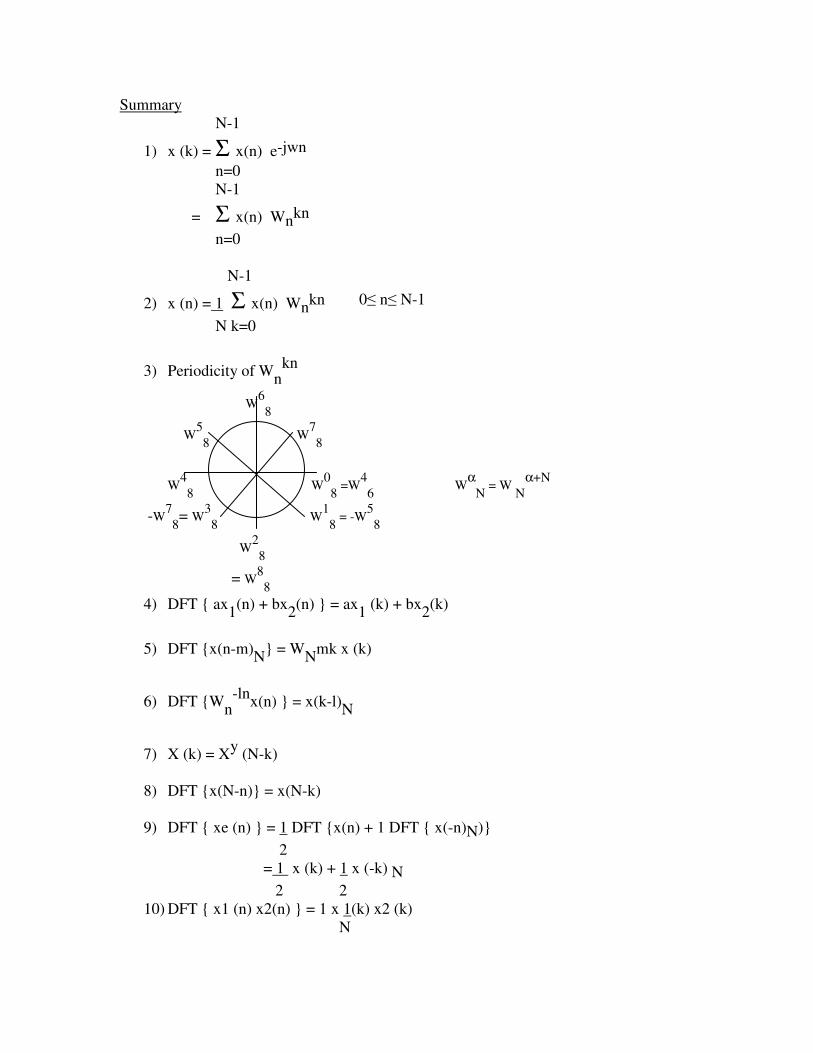
Summary
N-1
1) x (k) = Σ x(n) e-jwn
n=0
N-1
= Σ x(n) Wnkn
n=0
N-1
2) x (n) = 1 Σ x(n) Wnkn 0≤ n≤ N-1
N k=0
3) Periodicity of Wn
kn
W6
8
W5
8 W
7
8
W4
8 W
0
8 =W
4
6 W
α
N = W
N
α+N
-W7
8= W
3
8 W
1
8 = -W
5
8
W2
8
= W8
8
4) DFT { ax1
(n) + bx2
(n) } = ax1
(k) + bx2
(k)
5) DFT {x(n-m)N
} = WN
mk x (k)
6) DFT {Wn
-lnx(n) } = x(k-l)
N
7) X (k) = Xy (N-k)
8) DFT {x(N-n)} = x(N-k)
9) DFT { xe (n) } = 1 DFT {x(n) + 1 DFT { x(-n)N)}
2
= 1 x (k) + 1 x (-k) N
2 2
10) DFT { x1 (n) x2(n) } = 1 x 1(k) x2 (k)
N
Related Documents