Numerical investigation of an oceanic resonant regime induced by hurricane winds

Numerical investigation of an oceanic resonant regimeinduced by hurricane winds

Guillaume Samson & Hervé Giordani & Guy Caniaux &

Frank Roux

Received: 23 May 2008 /Accepted: 12 May 2009# Springer-Verlag 2009

Abstract The oceanic mixed layer (OML) response to anidealized hurricane with different propagation speeds isinvestigated using a two-layer reduced gravity oceanmodel. First, the model performances are examined withrespect to available observations relative to HurricaneFrances (2004). Then, 11 idealized simulations areperformed with a Holland (Mon Weather Rev 108(8):1212–1218, 1980) symmetric wind profile as surfaceforcing with storm propagation speeds ranging from 2 to12 m s−1. By varying this parameter, the phasing betweenatmospheric and oceanic scales is modified. Consequently,it leads to different momentum exchanges between thehurricane and the OML and to various oceanic responses.The present study determines how OML momentum andheat budgets depend on this parameter. The kinetic energyflux due to surface wind stress is found to strongly dependon the propagation speed and on the cross-track distance

from the hurricane center. A resonant regime betweensurface winds and near-inertial currents is clearly identi-fied. This regime maximizes locally the energy flux intothe OML. For fast-moving hurricanes (>6 m s−1), the ratioof kinetic energy converted into turbulence depends onlyon the wind stress energy input. For slow-movinghurricanes (<6 m s−1), the upwelling induced by currentdivergence enhances this conversion by shallowing theOML depth. Regarding the thermodynamic response, tworegimes are identified with respect to the propagationspeed. For slow-moving hurricanes, the upwelling com-bined with a sharp temperature gradient at the OML baseformed in the leading part of the storm maximizes theoceanic heat loss. For fast propagation speeds, theresonance mechanism sets up the cold wake on the rightside of the hurricane track. These results suggest that thepropagation speed is a parameter as important as thesurface wind speed to accurately describe the oceanicresponse to a moving hurricane.

Keywords Air–sea interactions . Oceanic mixed layer .

Hurricane propagation speed .

Entrainment parameterization . Upwelling .

Resonant regime . Near-inertial currents

1 Introduction

In hurricane conditions, the upper layers of the oceanreceive large amounts of kinetic energy and undergo astrong heat loss. The intense currents excited by thehurricane in the oceanic mixed layer (OML hereafter)generate turbulence by shear. This turbulence entrainscold waters from the thermocline into the OML. Thisprocess is mainly responsible for the local cooling

Ocean DynamicsDOI 10.1007/s10236-009-0203-8

Responsible Editor: Richard John Greatbatch

G. Samson :H. Giordani :G. CaniauxCentre National de Recherches Météorologiques,Groupe d’étude de l’Atmosphère Météorologique,Météo-France, CNRS,42 avenue Gaspard Coriolis,31057 Toulouse Cedex 01, France

G. Samson (*)Laboratoire de l’Atmosphère et des Cyclones,Université de La Réunion, Météo-France, CNRS,15 avenue René Cassin,97715 Saint-Denis Cedex 09, Francee-mail: [email protected]

F. RouxLaboratoire d’Aérologie, Université Toulouse 3, CNRS,14 avenue Edouard Belin,31400 Toulouse, France

observed in the oceanic wake of hurricanes (Price 1981;Sanford et al. 1987; Shay et al. 1992, among others). As aconsequence, the oceanic response is entirely forced by theamount of momentum transferred from the hurricane to theocean. In turn, the ocean response influences the hurricaneintensity (Schade 2000). It is therefore important to accu-rately represent this transfer of momentum and to understandhow the ocean responds to this strong energy input.

Two main reasons have been invoked to explain howhurricanes generate such strong oceanic responses. First,the very strong hurricane winds at surface level transferimportant amount of momentum into the ocean. Determin-ing the relationship between wind speed and momentumflux in high-wind regimes is a crucial point which has beenextensively studied from both theoretical (Emanuel 1986,1995, 2003) and experimental (Powell et al. 2003; Donelanet al. 2004; Black et al. 2006) approaches.

The second point is that the momentum flux does notdepend only on wind intensity but also on the phasingbetween the atmosphere and the ocean. The timescaleassociated with hurricane winds is imposed by thehurricane size—typically the radius of maximum wind(RMW hereafter)—and by the hurricane propagationspeed (UH hereafter). The timescale of the subtropicalOML is roughly equal to the local Coriolis frequency, f,but it also depends on its depth and the stratificationbelow. Scale analyses performed by Price (1981) andGreatbatch (1983) showed that hurricane winds changeover a timescale similar to the oceanic inertial frequency.More precisely, the transfer of momentum is maximizedon the right side of the hurricane track where winds andnear-inertial currents evolve cyclonically with closefrequencies, whereas the transfer of momentum is closeto zero on the left side where winds and currents evolve inan opposite way (Price 1981, 1983; Price et al. 1994).

The present study aims to explore how the OMLresponds to an idealized hurricane with different timescales.The timescales are investigated by varying the propagationspeed of the atmospheric forcing. The purpose is todetermine how the transfer of momentum varies and tounderstand how the OML momentum and heat budgets areaffected. The framework of this study is purely academic inorder to control the environment.

For this purpose, a simplified two-layer ocean model isused. Atmospheric (maximum wind, RMW) and oceanic(vertical density profile and latitude) parameters areidealized in order to isolate the role of the hurricanepropagation speed. This model is similar to those used byGeisler (1970), Chang and Anthes (1978), and Greatbatch(1983, among others) in their studies of the OML dynamicsand thermodynamics under a moving hurricane. InSection 2, the model is described and a simulation of theHurricane Frances on 4th September 2004 is compared

with observations collected during the CBLAST campaign(Black et al. 2006). This validation allows us to be fairlyconfident in the temperature and kinetic energy budgetspresented in the following sections. Section 3 describesthe experiments designed to explore the range of oceanicresponses with respect to hurricane propagation speedsvarying from 2 to 12 m s−1. The OML dynamics isinvestigated in Section 4 by quantifying the kinetic energybudget during the forcing period. Finally, the OML heatbudget is analyzed in Section 5 to identify the thermody-namic processes induced by different surface momentuminputs. Results are summarized and compared withprevious relevant studies in Section 6.

2 Description of the numerical model

2.1 Equations

The model used in this study is a two-layer reduced gravitymodel. The upper layer is an active layer where theprognostic equations are derived from the verticallyintegrated full-primitive equations system over the mixedlayer depth. The rigid lid approximation is made to simplifythe equations. This first layer overlies a motionless layerwhere the temperature and salinity profiles are representedby their vertical linear gradients. Because of the absence ofdynamics in the thermocline layer, this model is not able torepresent the vertical energy dispersion observed in theoceanic wake to the rear of hurricanes. This downwardpropagation is induced by the excitation of high baroclinicmodes and by the pressure gradient coupling between theOML and thermocline layers (Gill 1984; Shay et al. 1989,1992; Price et al. 1994). In this study, we only focus on theOML evolution during the forced stage, defined here as theperiod during which the surface winds induce a significantmomentum transfer into the OML, as opposed to therelaxation stage when the surface winds do not influencethe OML response anymore. As shown by Greatbatch(1984), horizontal currents stay confined within the OMLduring the forcing stage.

The conservations of momentum, heat, and salt for theOML are described by the following equations:

@U@t

þ f k � Uþ U Irð ÞU

¼ 1

r0

th� 1

r0rP � dU

hwe ð1Þ

@T

@tþ U I rð ÞT ¼ QS þ QL

r0CPh� dT

hwe ð2Þ

Ocean Dynamics

@S

@tþ U I rð ÞS ¼ E � P

h� dS

hwe ð3Þ

where h is the OML depth and U[u,v], T, and S are theOML depth-integrated horizontal current, temperature,salinity, respectively; ρ0 and Cp are the density and specificheat of seawater; τ is the wind stress vector; QS and QL arethe sensible and latent heat flux respectively; E and P arethe evaporation and precipitation; we is the entrainmentvelocity representing the turbulent mixing across the OMLbase; δ represents the discontinuity of the differentprognostic variables at the OML base; and k is the verticalunit vector and g the gravitational acceleration. Radiativefluxes and precipitation have second-order contributionscompared to the surface heat and moisture fluxes inducedby hurricane winds and are not taken into account here. Allthe model surface parameters are derived from the air–seaexchange bulk flux parameterization presented in Sec-tion 2.2. The horizontal pressure gradient in the OMLoverlying a motionless layer is expressed as:

rP ¼ g hrr� drrhð Þ ð4Þ

where ρ is the OML water density computed from aclassical linear state equation. The OML depth evolves byturbulent deepening and by vertical motions induced by thedivergence or the convergence of the OML currents. Itsprognostic equation is written as:

@h

@tþ U I rð Þh ¼ we � w�h ð5Þ

with

w�h ¼ 1

r0hr I U ð6Þ

and where w−h is the vertical velocity at the OML base andwe is the entrainment velocity calculated according to Gaspar(1988)'s parameterization based on the Niiler and Krauss(1977) general turbulent closure equation. This equation isderived from the turbulent kinetic equation (TKE) integratedover the OML depth and is written as (Gaspar 1988):

0:5 h dbwe ¼ m2u3� þ 0:5we du2 þ dv2

� �� 0:5 h BðhÞ� h "m ð7Þ

with

b ¼ g r0 � rð Þ=r0;m2 ¼ 2:6; BðhÞ ¼ QS þ QL

r0CPand "m

¼ E3=2m

�l

In this equation, the left-hand term represents thechange in potential energy due to the entrainment

velocity. The first term on the right-hand side is the netflux of TKE due to surface wind stress; this term isparameterized following Kraus and Turner (1967). Thesecond term is a source of TKE due to the vertical shear ofthe current at the OML base. This term was originallyparameterized as a function of u3� and did not resolveexplicitly the entrainment produced by the current shear atthe OML base. This parameterization weakness has beenpointed at by Jacob and Shay (2003) and is now replacedby the Niiler and Kraus (1977)'s formulation as written inEq. 7 which allows to explicitly represent the change in theentrainment velocity induced by the current shear. The thirdterm represents the surface buoyancy flux and the fourthterm is the TKE dissipation. εm is parameterized as afunction of the OML depth-integrated TKE, denoted Em,and of the dissipation length l following Kolmogorov(1942) and Garwood (1977). In Eq. 7, the same set ofconstants as in Gaspar (1988) is used. This modifiedparameterization allows us to obtain more realistic OMLdeepening and cooling in case of strong currents (seeSection 2.3).

In the second layer, the temperature stratification isspecified as a linear function (Price 1981; Bender et al.1993):

@T2@t

¼ weT2 � Trefh� zref

ð8Þ

where T2 is the second layer top temperature, Tref thetemperature at the base of the second layer, and zref is thedepth at the base of the second layer (200 m in oursimulations). The base of the second layer is kept fixedduring the simulations. Consequently, the evolution of T2depends only on the entrainment velocity and the OMLdepth. The same equation holds for the salinity. Thetemperature jump at the OML base is deduced from theOML temperature T and the second layer top temperatureT2 as follows:

dT ¼ T � T2: ð9ÞIn equations 1, 2, and 3, the prognostic variables are

staggered in space over a regular horizontal grid. Allprognostic variables are collocated at the same grid points.The horizontal advection is computed by using a second-order upstream scheme and the temporal derivative isdeduced from a first-order forward scheme. Model bound-aries are open, with horizontal relaxation toward the initialmodel density and depth profiles. With a horizontalresolution of 10 km and a time step of 15 min, the modelis unconditionally stable and is able to simulate over severaldays the OML response. As a consequence, it is welladapted to perform numerous simulations with differentatmospheric forcings.

Ocean Dynamics

2.2 Surface forcing and fluxes

Surface turbulent fluxes are computed using a parameterizationderived from flux measurements at sea (Weill et al. 2003). Thisprovides an accurate estimate of the different neutral-stability10-m exchange coefficients used in the conventional bulkaerodynamics formulas, for wind intensity up to 30 m s−1:

t ¼ raCd10nU10nU10n ð10Þ

QS ¼ raCpaCh10nU10nΔT10n ð11Þ

QL ¼ raLvaCe10nU10nΔq10n ð12Þρa is air density, Cpa the heat capacity of air, Lva the latentheat of vaporization, Cd10n the drag coefficient, Ch10n thesensible heat flux exchange coefficient, Ce10n the latent heatflux exchange coefficient, U10n the neutral equivalent windspeed at 10 m, ΔT10n the difference between the 10-m andsurface temperatures, and Δq10n the difference between the10-m and surface specific humidity.

Under hurricane conditions, recent field and laboratorymeasurements (Powell et al. 2003; Donelan et al. 2004;Makin 2005) and theoretical studies (Emanuel 1986, 1995)have shown that the transfer coefficients saturate (Cd10n

even declines) for high winds. This is related—but not asyet well understood—to the sea state not being fullydeveloped under hurricanes, to the flow separation mech-anism at waves crest, and to the generation of sea spray.Cd10n shows a clear dependence on the sea state (French etal. 2007), while Ce10n and Ch10n remain constant and showa weak sensitivity to the sea state (Drennan et al. 2007). Totake into account this saturation mechanism, the transfercoefficients are changed for wind speeds larger than 30 m s−1

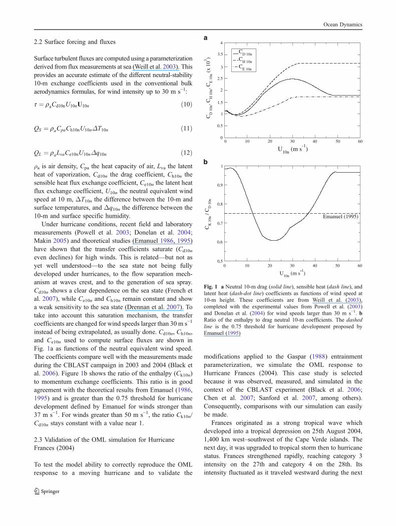
instead of being extrapolated, as usually done. Cd10n, Ch10n,and Ce10n used to compute surface fluxes are shown inFig. 1a as functions of the neutral equivalent wind speed.The coefficients compare well with the measurements madeduring the CBLAST campaign in 2003 and 2004 (Black etal. 2006). Figure 1b shows the ratio of the enthalpy (Ck10n)to momentum exchange coefficients. This ratio is in goodagreement with the theoretical results from Emanuel (1986,1995) and is greater than the 0.75 threshold for hurricanedevelopment defined by Emanuel for winds stronger than37 m s−1. For winds greater than 50 m s−1, the ratio Ck10n/Cd10n stays constant with a value near 1.

2.3 Validation of the OML simulation for HurricaneFrances (2004)

To test the model ability to correctly reproduce the OMLresponse to a moving hurricane and to validate the

modifications applied to the Gaspar (1988) entrainmentparameterization, we simulate the OML response toHurricane Frances (2004). This case study is selectedbecause it was observed, measured, and simulated in thecontext of the CBLAST experiment (Black et al. 2006;Chen et al. 2007; Sanford et al. 2007, among others).Consequently, comparisons with our simulation can easilybe made.

Frances originated as a strong tropical wave whichdeveloped into a tropical depression on 25th August 2004,1,400 km west–southwest of the Cape Verde islands. Thenext day, it was upgraded to tropical storm then to hurricanestatus. Frances strengthened rapidly, reaching category 3intensity on the 27th and category 4 on the 28th. Itsintensity fluctuated as it traveled westward during the next

Fig. 1 a Neutral 10-m drag (solid line), sensible heat (dash line), andlatent heat (dash-dot line) coefficients as functions of wind speed at10-m height. These coefficients are from Weill et al. (2003),completed with the experimental values from Powell et al. (2003)and Donelan et al. (2004) for wind speeds larger than 30 m s−1. bRatio of the enthalpy to drag neutral 10-m coefficients. The dashedline is the 0.75 threshold for hurricane development proposed byEmanuel (1995)

Ocean Dynamics

several days. It passed north of the Antilles on 1stSeptember, struck the Bahamas on 2nd–3rd September,and made first landfall in south-central Florida on 4thSeptember. Late on 5th September, it reached the Gulf ofMexico near Tampa as a tropical storm and, after a shorttrip over water, it landed again in the Florida Panhandle,headed north, and weakened to tropical depression whilecausing heavy rainfall in the southern and eastern USA andin the eastern Canada.

The numerical simulation lasts from 00 UTC on 31stAugust 2004 until 00 UTC on 4th September. The modeldomain extends from 18° N to 28° N and from 62° W to78° W, which includes the National Hurricane Center besttrack for Frances during this period. During the first 2 days,Frances underwent a series of eyewall replacement cycleswhile moving west–northwestward, but it remained acategory 4 storm. Over the two following days, Franceswas affected by westerly wind shear, and it weakened tocategory 3 (100–110 kt winds) on 2th–3th September nearof the Bahamas, then to a category 2 system (85–90 kt) on3rd–4th September. An airborne deployment of floats anddrifters took place on 31st August ahead of the hurricaneand captured its cold wake with unprecedented precision.The details of the experiment, measurements, and oceanicresponse can be found in D'Asaro et al. (2007).

The pre-storm vertical profiles of temperature and salinitymeasured by an autonomous profiling float about 55 km tothe right of the hurricane track (Sanford et al. 2007) are usedto initialize the model. The OML depth diagnosed from thisprofile using a 0.2°C jump criterion is equal to 40 m. Theinitial variables are deduced from the profiles averaged overthe OML depth. The temperature and temperature jump, δT,obtained are 29.26°C and 0.76°C, respectively, and thesalinity and salinity jump, δS, obtained are 36.33 and −0.38,respectively. As deduced from the measured profile, thedepth and temperature at the second layer base in Eq. 8 aretaken as: zref=200 m and Tref=21°C, respectively.

To take into account the spatial variations of the pre-storm sea surface temperature (SST) in the simulationdomain, a blended SST analysis of the 31st August with a0.1° resolution, provided by the Centre de MétéorologieSpatiale (Météo-France, Lannion, France), is used. Thethermocline temperature gradient is then corrected to matchthe 200-m temperature Tref measured by the float andchosen as reference. Because of weak pre-hurricanecurrents (≤0.2 m s−1), initial currents are ignored and theOML model is initially at rest. To represent the atmosphericforcing, we use the “HWIND” 10-m wind analysis with a0.1° horizontal resolution and a 6-h temporal resolutionfrom Hurricane Research Division (HRD, NOAA/AOML,Miami, FL, USA; Powell et al. 1998). This analysisaccurately represents the hurricane surface wind field andtakes into account the changes of wind intensity and

structure by integrating the satellite and in situ measure-ments made during CBLAST. A linear interpolation isperformed between two successive analyses to avoid anyabrupt change in the wind field used to force the oceanmodel. The wind field is then moved over the OML modelwith a propagation speed deduced from the 6-h NationalHurricane Center best track.

The OML model temperature and currents responseexcited by Frances after a 5-day integration period are shownin Fig. 2a. Strong near-inertial currents are observed on theright side of the hurricane track with an intensity reaching1.5 m s−1 below the hurricane and 1 m s−1 just after itspassage. The currents extend to roughly 150 km from thehurricane track. Divergence and convergence are alternative-ly created by the quasi-inertially rotating currents behind thestorm. The wavelength of these simulated inertial waves isabout 500 km, which compares well with the along-trackcharacteristic scale from Greatbatch (1984): 2π UH/f=525 km for a latitude of 23° and a mean propagation speedUH of 4.8 m s−1. The intensity and structure of the oceaniccurrents shown in Fig. 2 compare reasonably well with theresults of simulations obtained by Chen et al. (2007).

The temperature in the OML is strongly affected byFrances as well. The coolest waters, with SST perturbationsof −2°C to −3.5°C, are observed where the strongestcurrents are generated, to the right of the hurricane track.Cooling from −0.5°C to −1°C, mainly generated by wind-stress-induced turbulence and surface heat fluxes, isobserved in regions where near-inertial currents and shearinstabilities are weak, on the left side. A zone of colderwaters (ΔSST ≈ −3.5°C) at 24–26° N, 73–76° W is alsoclearly observed in the TMI1/AMSR-E2 SST analysisproduct (GHRSST-PP3 project, Donlon et al. 2007) and inthe simulated SST field on 5th September with a goodagreement in location, coverage, and intensity (Fig. 2b).This local cooling took place between 12 UTC on 2ndSeptember and 00 UTC on 4th September when Francesreached its maximal intensity (935 hPa and 120–125 kt) atabout 07 UTC on 1st September, then decreased to category3 (100–110 kt) on 2nd–3rd September and category 2 (85–90 kt) on 3rd–4th September. However, the hurricanepropagation speed slowed down from 5.5 m s−1 on 1stSeptember to 3.8 m s−1 on 3rd September.

The OML simulated response is also compared locally withthe vertical profiles measured by the autonomous profilingfloat 55 km to the right of the hurricane track (at about 22.2°N, 70.0°W) just after the passage of Frances at 17 UTC on 1stSeptember (see Table 1). The OML depth-integrated maxi-mum cooling and currents deduced from the vertical profilescompare well with the simulated ones, with, however, anunderestimation of 12.5% for the current and an overestima-tion of 4.3% for the cooling. The maximum simulated OMLdepth is also in good agreement with the measured one with

Ocean Dynamics

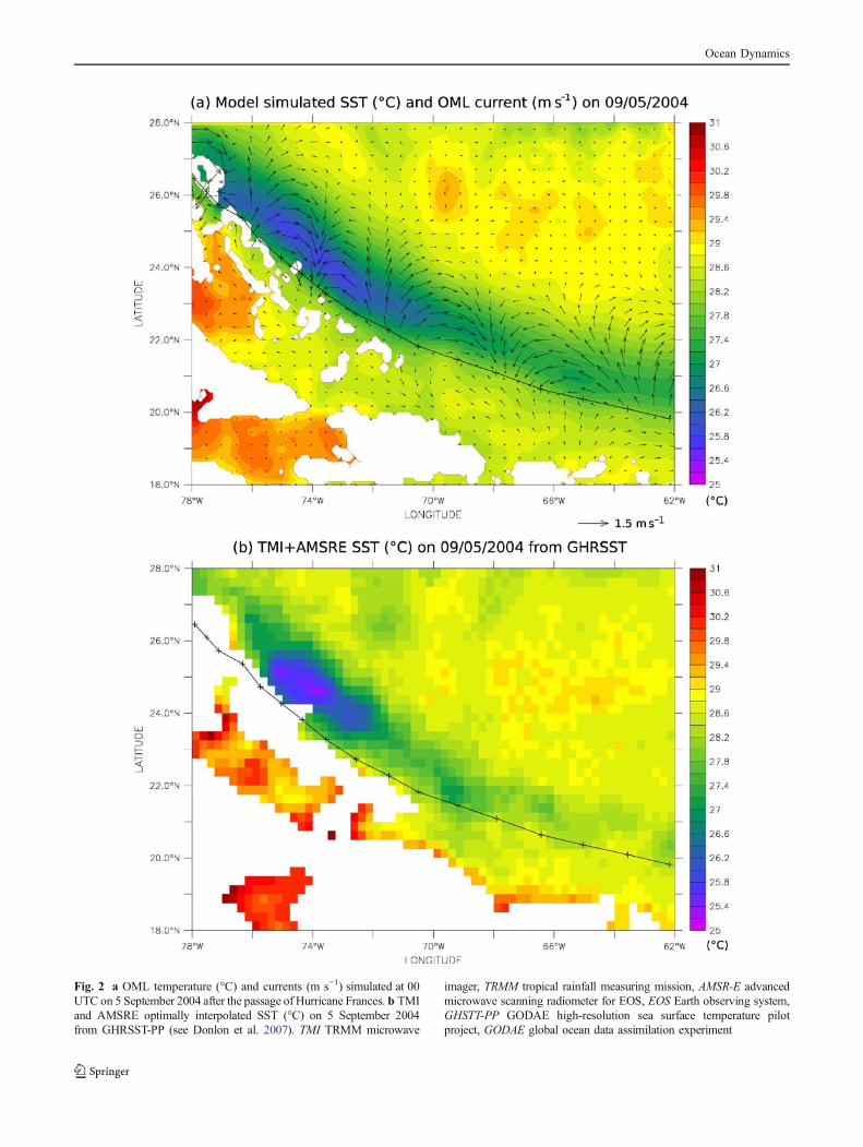
Fig. 2 a OML temperature (°C) and currents (m s−1) simulated at 00UTC on 5 September 2004 after the passage of Hurricane Frances. b TMIand AMSRE optimally interpolated SST (°C) on 5 September 2004from GHRSST-PP (see Donlon et al. 2007). TMI TRMM microwave

imager, TRMM tropical rainfall measuring mission, AMSR-E advancedmicrowave scanning radiometer for EOS, EOS Earth observing system,GHSTT-PP GODAE high-resolution sea surface temperature pilotproject, GODAE global ocean data assimilation experiment

Ocean Dynamics

a weak underestimation of 8.3%. This shows that the modelreproduces realistically both the dynamical and thermody-namical OML responses to Frances. It is difficult to preciselydetermine the reasons for the model errors considering theuncertainties in the atmospheric forcing and the surfacefluxes coefficients (the precision of float measurements isabout 0.02 m s−1). Another source of error can be the neglectof pre-hurricane currents in our simulation. The currentswere weaker than 0.2 m s−1 and could have slightlyinfluenced the OML response. Despite these uncertainties,the model skills are robust and compare reasonably well withother multilayer models skills (e.g., Price 1983).

This validation indicates that the present OML model andits entrainment parameterization correctly represent thestructure and amplitude of the OML dynamic and thermody-namic fields during this hurricane forcing event. When theoriginal version of the Gaspar (1988)'s entrainment parame-terization is used, the dynamically induced cooling is stronglyunderestimated (not shown) and does not produce anasymmetrical cooling on either side of the hurricane track.This result highlights and confirms the importance ofaccurately representing the shear-induced mixing to obtainrealistic OML response in hurricane conditions. As theoceanic thermal and dynamical responses induced byHurricane Frances were realistically simulated, the model isnow used to investigate how the OML depends on the phasingbetween hurricane winds and OML near-inertial currents.

3 Experimental design

In this section, a set of idealized experiments is designed toexplore a large range of OML responses to idealizedhurricane forcings. Consequently, all the atmospheric andoceanic parameters of the model are kept constant, exceptfor the hurricane propagation speed UH.

3.1 Initial and boundary conditions

Atmospheric parameters are set to values typical ofhurricanes regions: the 2-m air temperature is fixed at 26°C

and the 2-m relative humidity at 85%. Surface winds arerepresented by an idealized axisymmetric and steady windfield of a typical (category 3) hurricane using the Holland(1980) wind profile with a maximum wind of 50 m s−1 and aRMW of 60 km, which corresponds to a central pressure ofabout 960 hPa. The surface wind field intensity is presentedin Appendix, Fig. 16. A uniform inflow angle of 15° isimposed to represent the convergent radial component of thesurface wind field. This axisymmetric wind field is movedwestward over the oceanic domain at a constant latitude of30° N. The local inertial period at this latitude is about 24 h.Previous studies have examined the effect of wind asymme-try induced by hurricane propagation on the OML response.Chang and Anthes (1978) observed that the global currentand temperature patterns remain similar whether a propaga-tion speed of 5 m s−1 is taken into account or not. Price(1981) showed that for maximum winds of 35 m s−1 and apropagation speed of 8.5 m s−1, this asymmetric componentenhances the SST cooling by 15% on the right-hand side ofthe hurricane track. Simulations taking into account thiseffect conducted with our model confirm these previousresults (the most asymmetric case is presented in Appendix).We found that asymmetry has only a minor impact on theintensity of the OML thermodynamical and dynamicalresponse. Furthermore, the wind–current couplingmechanismis not altered by the asymmetric wind field. Consequently, thestructure of the OML thermodynamical and dynamicalresponse is not modified when the asymmetric wind field isused. According to these results, we chose not to include thisasymmetry in the wind field to study the resonant regime.With this hypothesis, all the OML simulations presented hereare forced with the same wind field. The different regimes ofoceanic responses described hereafter are therefore onlyinduced by changes in the propagation speed of the storm.

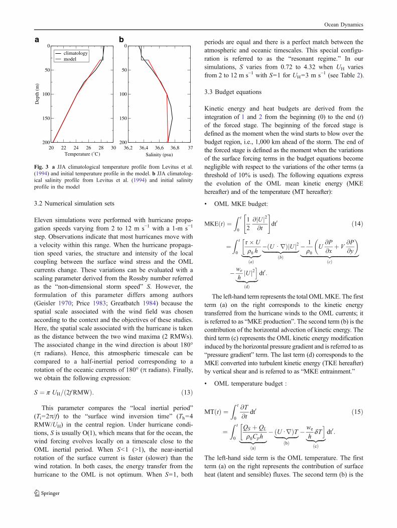
The model surface fluxes are calculated following themethod described in Section 2.2 at every time step to takeinto account the model SST evolution. The initializationprocedure uses June–July–August averaged climatologicaltemperature and salinity profiles from Levitus et al. (1994)averaged over the typical North Atlantic hurricane region(20–30° N, 60–80° W; Fig. 3). The initial values in theOML model are deduced from these profiles. The initialOML temperature (Fig. 3a) is 28.4°C, corresponding to anair–sea temperature difference of 2.4°C, with an OMLdepth of 30 m and a temperature jump of 0.7°C at the OMLbase. Initial OML salinity (Fig. 3b) is set to 36.4 with asalinity jump of −0.1. These values are representative of theOML during the hurricane season over the tropical Atlantic.A Tref (see Eq. 8) temperature of 20.3°C and a Sref salinityof 36.7 at a reference depth Zref of 200 m are used tocalculate the vertical density gradient representing theupper thermocline and the density jump at the OML base.The ocean is initially horizontally homogeneous and at rest.

Table 1 Observed (from Sanford et al. 2007; D'Asaro et al. 2007) andsimulated characteristics of the OML response to Hurricane Frances(2004)

EM-APEX data 2-layer model differencesOMLmean values OML bulk values

OML depth, h (m) 120 m 110 m -8.3 %

OML cooling,ΔT (°C)

-2.2°C -2.3°C +4.3 %

OML current,U, V (m s−1)

1.6 1.4 -12.5 %

Ocean Dynamics

3.2 Numerical simulation sets

Eleven simulations were performed with hurricane propa-gation speeds varying from 2 to 12 m s−1 with a 1-m s−1

step. Observations indicate that most hurricanes move witha velocity within this range. When the hurricane propaga-tion speed varies, the structure and intensity of the localcoupling between the surface wind stress and the OMLcurrents change. These variations can be evaluated with ascaling parameter derived from the Rossby number referredas the “non-dimensional storm speed” S. However, theformulation of this parameter differs among authors(Geisler 1970; Price 1983; Greatbatch 1984) because thespatial scale associated with the wind field was chosenaccording to the context and the objectives of these studies.Here, the spatial scale associated with the hurricane is takenas the distance between the two wind maxima (2 RMWs).The associated change in the wind direction is about 180°(π radians). Hence, this atmospheric timescale can becompared to a half-inertial period corresponding to arotation of the oceanic currents of 180° (π radians). Finally,we obtain the following expression:

S ¼ p UH= 2f RMWð Þ: ð13Þ

This parameter compares the “local inertial period”(Ti=2π/f) to the “surface wind inversion time” (Th=4RMW/UH) in the central region. Under hurricane condi-tions, S is usually O(1), which means that for the ocean, thewind forcing evolves locally on a timescale close to theOML inertial period. When S<1 (>1), the near-inertialrotation of the surface current is faster (slower) than thewind rotation. In both cases, the energy transfer from thehurricane to the OML is not optimum. When S=1, both

periods are equal and there is a perfect match between theatmospheric and oceanic timescales. This special configu-ration is referred to as the “resonant regime.” In oursimulations, S varies from 0.72 to 4.32 when UH variesfrom 2 to 12 m s−1 with S=1 for UH=3 m s−1 (see Table 2).

3.3 Budget equations

Kinetic energy and heat budgets are derived from theintegration of 1 and 2 from the beginning (0) to the end (t)of the forced stage. The beginning of the forced stage isdefined as the moment when the wind starts to blow over thebudget region, i.e., 1,000 km ahead of the storm. The end ofthe forced stage is defined as the moment when the variationsof the surface forcing terms in the budget equations becomenegligible with respect to the variations of the other terms (athreshold of 10% is used). The following equations expressthe evolution of the OML mean kinetic energy (MKEhereafter) and of the temperature (MT hereafter):

& OML MKE budget:

MKEðtÞ ¼Z t

0

1

2

@ Uj j2@t

" #dt0

¼Z t

0

t � U

r0 h

�|fflfflfflffl{zfflfflfflffl}

ðaÞ

� U I rð Þ Uj j2|fflfflfflfflfflfflfflfflfflffl{zfflfflfflfflfflfflfflfflfflffl}ðbÞ

� 1

r0U

@P

@xþ V

@P

@y

� �|fflfflfflfflfflfflfflfflfflfflfflfflfflfflfflfflfflffl{zfflfflfflfflfflfflfflfflfflfflfflfflfflfflfflfflfflffl}

ðcÞ

� we

hUj j2

i|fflfflfflfflffl{zfflfflfflfflffl}

dð Þ

dt0:

ð14Þ

The left-hand term represents the total OMLMKE. The firstterm (a) on the right corresponds to the kinetic energytransferred from the hurricane winds to the OML currents; itis referred to as “MKE production”. The second term (b) is thecontribution of the horizontal advection of kinetic energy. Thethird term (c) represents the OML kinetic energy modificationinduced by the horizontal pressure gradient and is referred to as“pressure gradient” term. The last term (d) corresponds to theMKE converted into turbulent kinetic energy (TKE hereafter)by vertical shear and is referred to as “MKE entrainment.”

& OML temperature budget :

MTðtÞ ¼Z t

0

@T

@tdt0

¼Z t

0

QS þ QL

r0Cph

�|fflfflfflfflfflffl{zfflfflfflfflfflffl}

að Þ

� U Irð ÞT|fflfflfflfflffl{zfflfflfflfflffl}bð Þ

� we

hdT

i|fflfflffl{zfflfflffl}

cð Þ

dt0:

ð15Þ

The left-hand side term is the OML temperature. The firstterm (a) on the right represents the contribution of surfaceheat (latent and sensible) fluxes. The second term (b) is the

20 22 24 26 28 30Temperature (˚C)

0

50

100

150

200

Dep

th (

m)

climatologymodel

36,2 36,4 36,6 36,8 37Salinity (psu)

0

50

100

150

200

Fig. 3 a JJA climatological temperature profile from Levitus et al.(1994) and initial temperature profile in the model. b JJA climatolog-ical salinity profile from Levitus et al. (1994) and initial salinityprofile in the model

Ocean Dynamics

contribution of the horizontal advection of heat. The thirdterm (c) is associated with the turbulent entrainment at theOML base and is referred to as “T entrainment” hereafter.

The budgets are calculated along the cross-track section(defined as the x-axis, positive to the right of the track) inthe central part of the simulation domain (“budget line” inFig. 4). This line is divided into seven 1-RMW (60-km)-

Fig. 4 Scheme representing theexperimental design, the modeldomain dimensions, the spatialaxes, and the budget line

Fig. 5 Scalar product [τ × U]/ρ (m3 s−3) for propagation speeds from2 to 12 m s−1. White contours are the cosine of the angle between thewind and current vectors, the solid (dashed) contours denote positive

(negative) values, the contour interval is 0.3. Black contours indicatethe 10-m s−1 isotachs of the surface wind

Ocean Dynamics

long segments corresponding to different distances from thehurricane center, from −3 RMW to +3 RMW (−180to +180 km). The wind speed is larger than 20 m s−1 forall segments. The budget terms are averaged over thesesegments in order to show representative values. Theperpendicular y-axis is positive in the direction opposite tothe hurricane propagation.

4 OML mean kinetic energy budget

4.1 Instantaneous wind energy flux

To compare the simulation behavior with the storm speedparameter S defined in Section 3.2, the scalar product τ ×U/ρ (where τ and U are the surface wind stress and theOML current vectors, respectively, and ρ is the OMLdensity) is presented in Fig. 5 for different propagationspeeds. This term represents the local and instantaneouskinetic energy flux transferred from the surface wind to theOML current. It is referred to as the “wind–currentcoupling” and is expressed in m3 s−3.

Positive values are observed for all simulations (Fig. 5).The positive region is well correlated with the zones wherethe winds are strong and nearly oriented along the directionof the currents. Its position and intensity vary according toUH. As UH increases, the positive zone moves from therear-left quadrant to the right quadrant of the hurricane withan anticlockwise rotation. This zone is larger and extendsfurther to the right of the hurricane when the propagation isfaster. When UH increases from 2 to 6 m s−1, its intensityincreases quickly, then it decreases slightly for fasterpropagation speeds. The maximum value is observed inthe rear-right quadrant for UH=5 m s−1 which is slightlylarger than the value deduced from the “non-dimensionalstorm speed” S=1. An explanation of this behavior is givenin Section 4.2.

When the hurricane moves faster than 4 m s−1, the windand current become perpendicular in some regions, whichleads to substantial reduction in the energy transfers. Theregion with negative values corresponds to a zone wherethe OML current is decelerated by the surface winds. Thenegative wind energy flux is two times weaker than thepositive one and is less sensitive to the hurricanepropagation speed. Its position moves anticlockwise fromfront to rear-left quadrant with increasing UH (Fig. 5).

Figure 5 gives some details about the complex relation-ship between the surface winds and the OML currents. Thekinetic energy flux from the hurricane to the OML is spatiallyheterogeneous, and its structure and amplitude stronglydepend on the hurricane propagation speed. The next sectionlooks precisely at the whole OML kinetic energy budget inorder to understand how the modification of the surfacekinetic energy flux affects the OML dynamic response.

4.2 OML mean kinetic energy production and entrainment

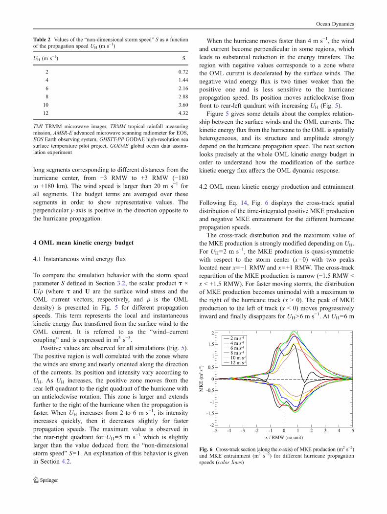
Following Eq. 14, Fig. 6 displays the cross-track spatialdistribution of the time-integrated positive MKE productionand negative MKE entrainment for the different hurricanepropagation speeds.

The cross-track distribution and the maximum value ofthe MKE production is strongly modified depending on UH.For UH=2 m s−1, the MKE production is quasi-symmetricwith respect to the storm center (x=0) with two peakslocated near x=−1 RMW and x=+1 RMW. The cross-trackrepartition of the MKE production is narrow (−1.5 RMW <x < +1.5 RMW). For faster moving storms, the distributionof MKE production becomes unimodal with a maximum tothe right of the hurricane track (x > 0). The peak of MKEproduction to the left of track (x < 0) moves progressivelyinward and finally disappears for UH>6 m s−1. At UH=6 m

Table 2 Values of the “non-dimensional storm speed” S as a functionof the propagation speed UH (m s−1)

UH (m s−1) S

2 0.72

4 1.44

6 2.16

8 2.88

10 3.60

12 4.32

TMI TRMM microwave imager, TRMM tropical rainfall measuringmission, AMSR-E advanced microwave scanning radiometer for EOS,EOS Earth observing system, GHSTT-PP GODAE high-resolution seasurface temperature pilot project, GODAE global ocean data assimi-lation experiment

-5 -4 -3 -2 -1 0 1 4 5

-2

-1,5

-1

-0,5

0

0,5

1

1,5

22 m s 1

4 m s 1

6 m s 1

8 m s 1

10 m s 1

12 m s 1

2 3

Fig. 6 Cross-track section (along the x-axis) of MKE production (m2 s−2)and MKE entrainment (m2 s−2) for different hurricane propagationspeeds (color lines)

Ocean Dynamics

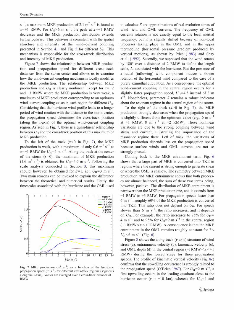
s−1, a maximum MKE production of 2.1 m2 s−2 is found atx=+1 RMW. For UH>6 m s−1, the peak at x=+1 RMWdecreases and the MKE production distribution extendsfurther outward. This behavior is consistent with the spatialstructure and intensity of the wind–current couplingpresented in Section 4.1 and Fig. 5 for different UH. Thismechanism is responsible for the cross-track distributionand intensity of MKE production.

Figure 7 shows the relationship between MKE produc-tion and propagation speed for different cross-trackdistances from the storm center and allows us to examinehow the wind–current coupling mechanism locally modifiesthe MKE production. The relationship between MKEproduction and UH is clearly nonlinear. Except for x=−2and −3 RMW where the MKE production is very weak, amaximum of MKE production corresponding to an optimumwind–current coupling exists in each region for different UH.Considering that the hurricane wind profile leads to a longerperiod of wind rotation with the distance to the storm center,the propagation speed determines the cross-track position(along the x-axis) of the optimal wind–current couplingregion. As seen in Fig. 7, there is a quasi-linear relationshipbetween UH and the cross-track position of this maximum ofMKE production.

To the left of the track (x<0 in Fig. 7), the MKEproduction is weak, with a maximum of only 0.6 m2 s−2 atx=−1 RMW for UH=4 m s−1. Along the track at the centerof the storm (x=0), the maximum of MKE production(1.6 m2 s−2) is obtained for UH=4.5 m s−1. Following thescale analysis conducted in Section 3, this maximumshould, however, be obtained for S=1, i.e., UH=3 m s−1.Two main reasons can be invoked to explain the differencebetween the theoretical and numerical results. Firstly, thetimescales associated with the hurricane and the OML used

to calculate S are approximations of real evolution times ofwind field and OML currents. The frequency of OMLcurrents rotation is not exactly equal to the local inertialfrequency, but it is slightly shifted because of non-localprocesses taking place in the OML and in the upperthermocline (horizontal pressure gradient produced byvertical motions), as shown by Price (1983) and Shayet al. (1992). Secondly, we supposed that the wind rotatesby 180° over a distance of 2 RMW to define the lengthscale, L, associated with the hurricane. But the presence ofa radial (inflowing) wind component induces a slowerrotation of the horizontal wind compared to the case of apurely azimuthal circulation. As a consequence, the optimalwind–current coupling in the central region occurs for aslightly faster propagation speed, UH=4.5 instead of 3 ms−1. Nonetheless, parameter S remains a robust indicatorabout the resonant regime in the central region of the storm.

To the right of the track (x>0 in Fig. 7), the MKEproduction strongly decreases when the propagation speedis slightly different from the optimum value (e.g., 6 m s−1

at +1 RMW, 8 m s−1 at +2 RMW). These nonlinearvariations are due to the strong coupling between windstress and current, illustrating the importance of theresonance regime there. Left of track, the variations ofMKE production depends less on the propagation speedbecause surface winds and OML currents are not sostrongly phased.

Coming back to the MKE entrainment term, Fig. 6shows that a large part of MKE is converted into TKE inregions where the current is strong enough to generate shearor where the OML is shallow. The symmetry between MKEproduction and MKE entrainment shows that both process-es are almost balanced, the sum of these two terms being,however, positive. The distribution of MKE entrainment isnarrower than the MKE production one, and it extends from−1 RMW to +3 RMW. For propagation speeds faster than6 m s−1, roughly 60% of the MKE production is convertedinto TKE. This ratio does not depend on UH. For speedsslower than 6 m s−1, the ratio increases, and it dependson UH. For example, the ratio increases to 75% for UH=4 m s−1 and to 95% for UH=2 m s−1 in the central region(−1 RMW< x < +1RMW). A consequence is that the MKEentrainment in the OML remains roughly constant for 2<UH<6 m s−1 (Fig. 6).

Figure 8 shows the along-track (y-axis) structure of windstress (a), entrainment velocity (b), kinematic velocity (c),and OML depth (d) in the central region (−1RMW< x <+1RMW) during the forced stage for three propagationspeeds. The profile of kinematic vertical velocity (Fig. 8c)confirms that the upwelling occurrence is strongly related tothe propagation speed (O’Brien 1967). For UH=2 m s−1, afirst upwelling occurs in the leading quadrant close to thehurricane center (y ≈ −10 km), whereas for UH=4 and

0 1 4 5 6 7 10 11 12 13 140

0,5

1

1,5

20 RMW+1 RMW+2 RMW+3 RMW-1 RMW-2 RMW-3 RMW

32 98

Fig. 7 MKE production (m2 s−2) as a function of the hurricanepropagation speed (m s−1) for different cross-track regions (segmentsalong the x-axis). Values are averaged over a cross-track distance of 1RMW

Ocean Dynamics

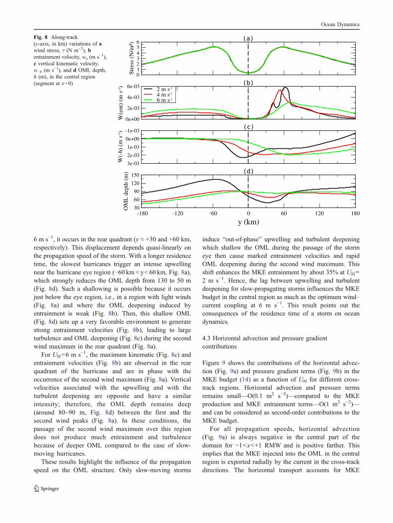
6 m s−1, it occurs in the rear quadrant (y ≈ +30 and +60 km,respectively). This displacement depends quasi-linearly onthe propagation speed of the storm. With a longer residencetime, the slowest hurricanes trigger an intense upwellingnear the hurricane eye region (−60 km < y< 60 km, Fig. 8a),which strongly reduces the OML depth from 130 to 50 m(Fig. 8d). Such a shallowing is possible because it occursjust below the eye region, i.e., in a region with light winds(Fig. 8a) and where the OML deepening induced byentrainment is weak (Fig. 8b). Then, this shallow OML(Fig. 8d) sets up a very favorable environment to generatestrong entrainment velocities (Fig. 8b), leading to largeturbulence and OML deepening (Fig. 8c) during the secondwind maximum in the rear quadrant (Fig. 8a).

For UH=6 m s−1, the maximum kinematic (Fig. 8c) andentrainment velocities (Fig. 8b) are observed in the rearquadrant of the hurricane and are in phase with theoccurrence of the second wind maximum (Fig. 8a). Verticalvelocities associated with the upwelling and with theturbulent deepening are opposite and have a similarintensity; therefore, the OML depth remains deep(around 80–90 m, Fig. 8d) between the first and thesecond wind peaks (Fig. 8a). In these conditions, thepassage of the second wind maximum over this regiondoes not produce much entrainment and turbulencebecause of deeper OML compared to the case of slow-moving hurricanes.

These results highlight the influence of the propagationspeed on the OML structure. Only slow-moving storms

induce “out-of-phase” upwelling and turbulent deepeningwhich shallow the OML during the passage of the stormeye then cause marked entrainment velocities and rapidOML deepening during the second wind maximum. Thisshift enhances the MKE entrainment by about 35% at UH=2 m s−1. Hence, the lag between upwelling and turbulentdeepening for slow-propagating storms influences the MKEbudget in the central region as much as the optimum wind–current coupling at 6 m s−1. This result points out theconsequences of the residence time of a storm on oceandynamics.

4.3 Horizontal advection and pressure gradientcontributions

Figure 9 shows the contributions of the horizontal advec-tion (Fig. 9a) and pressure gradient terms (Fig. 9b) in theMKE budget (14) as a function of UH for different cross-track regions. Horizontal advection and pressure termsremains small—O(0.1 m2 s−2)—compared to the MKEproduction and MKE entrainment terms—O(1 m2 s−2)—and can be considered as second-order contributions to theMKE budget.

For all propagation speeds, horizontal advection(Fig. 9a) is always negative in the central part of thedomain for −1<x<+1 RMW and is positive farther. Thisimplies that the MKE injected into the OML in the centralregion is exported radially by the current in the cross-trackdirections. The horizontal transport accounts for MKE

Fig. 8 Along-track(y-axis, in km) variations of awind stress, τ (N m−2), bentrainment velocity, we (m s−1),c vertical kinematic velocity,w−h (m s−1), and d OML depth,h (m), in the central region(segment at x=0)

Ocean Dynamics

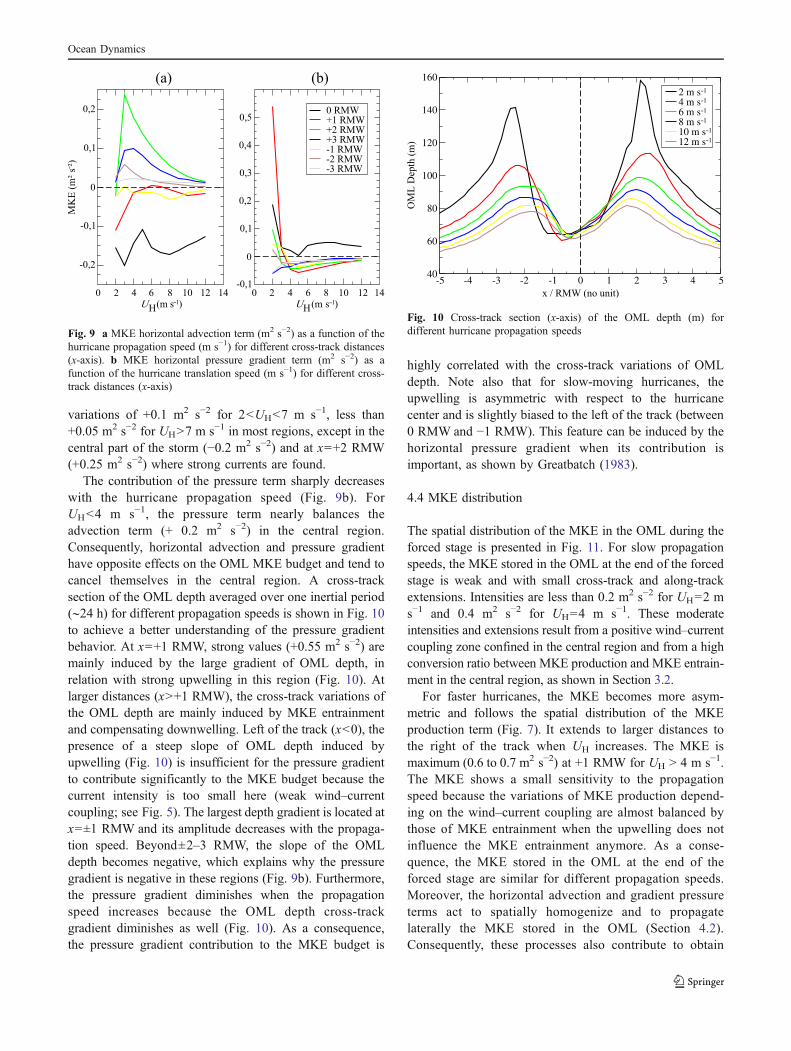
variations of +0.1 m2 s−2 for 2<UH<7 m s−1, less than+0.05 m2 s−2 for UH>7 m s−1 in most regions, except in thecentral part of the storm (−0.2 m2 s−2) and at x=+2 RMW(+0.25 m2 s−2) where strong currents are found.

The contribution of the pressure term sharply decreaseswith the hurricane propagation speed (Fig. 9b). ForUH<4 m s−1, the pressure term nearly balances theadvection term (+ 0.2 m2 s−2) in the central region.Consequently, horizontal advection and pressure gradienthave opposite effects on the OML MKE budget and tend tocancel themselves in the central region. A cross-tracksection of the OML depth averaged over one inertial period(∼24 h) for different propagation speeds is shown in Fig. 10to achieve a better understanding of the pressure gradientbehavior. At x=+1 RMW, strong values (+0.55 m2 s−2) aremainly induced by the large gradient of OML depth, inrelation with strong upwelling in this region (Fig. 10). Atlarger distances (x>+1 RMW), the cross-track variations ofthe OML depth are mainly induced by MKE entrainmentand compensating downwelling. Left of the track (x<0), thepresence of a steep slope of OML depth induced byupwelling (Fig. 10) is insufficient for the pressure gradientto contribute significantly to the MKE budget because thecurrent intensity is too small here (weak wind–currentcoupling; see Fig. 5). The largest depth gradient is located atx=±1 RMW and its amplitude decreases with the propaga-tion speed. Beyond±2–3 RMW, the slope of the OMLdepth becomes negative, which explains why the pressuregradient is negative in these regions (Fig. 9b). Furthermore,the pressure gradient diminishes when the propagationspeed increases because the OML depth cross-trackgradient diminishes as well (Fig. 10). As a consequence,the pressure gradient contribution to the MKE budget is

highly correlated with the cross-track variations of OMLdepth. Note also that for slow-moving hurricanes, theupwelling is asymmetric with respect to the hurricanecenter and is slightly biased to the left of the track (between0 RMW and −1 RMW). This feature can be induced by thehorizontal pressure gradient when its contribution isimportant, as shown by Greatbatch (1983).

4.4 MKE distribution

The spatial distribution of the MKE in the OML during theforced stage is presented in Fig. 11. For slow propagationspeeds, the MKE stored in the OML at the end of the forcedstage is weak and with small cross-track and along-trackextensions. Intensities are less than 0.2 m2 s−2 for UH=2 ms−1 and 0.4 m2 s−2 for UH=4 m s−1. These moderateintensities and extensions result from a positive wind–currentcoupling zone confined in the central region and from a highconversion ratio between MKE production and MKE entrain-ment in the central region, as shown in Section 3.2.

For faster hurricanes, the MKE becomes more asym-metric and follows the spatial distribution of the MKEproduction term (Fig. 7). It extends to larger distances tothe right of the track when UH increases. The MKE ismaximum (0.6 to 0.7 m2 s−2) at +1 RMW for UH > 4 m s−1.The MKE shows a small sensitivity to the propagationspeed because the variations of MKE production depend-ing on the wind–current coupling are almost balanced bythose of MKE entrainment when the upwelling does notinfluence the MKE entrainment anymore. As a conse-quence, the MKE stored in the OML at the end of theforced stage are similar for different propagation speeds.Moreover, the horizontal advection and gradient pressureterms act to spatially homogenize and to propagatelaterally the MKE stored in the OML (Section 4.2).Consequently, these processes also contribute to obtain

0 4 6 8 10 14

-0,2

-0,1

0

0,1

0,2

0 4 6 8 12 14-0,1

0

0,1

0,2

0,3

0,4

0,50 RMW+1 RMW+2 RMW+3 RMW-1 RMW-2 RMW-3 RMW

2 12 2 10

HH

Fig. 9 a MKE horizontal advection term (m2 s−2) as a function of thehurricane propagation speed (m s−1) for different cross-track distances(x-axis). b MKE horizontal pressure gradient term (m2 s−2) as afunction of the hurricane translation speed (m s−1) for different cross-track distances (x-axis)

-5 -4 -3 -2 -1 0 1 2 4 540

60

80

100

120

140

160

2 m s 14 m s 16 m s 18 m s 110 m s 112 m s 1

3

Fig. 10 Cross-track section (x-axis) of the OML depth (m) fordifferent hurricane propagation speeds

Ocean Dynamics

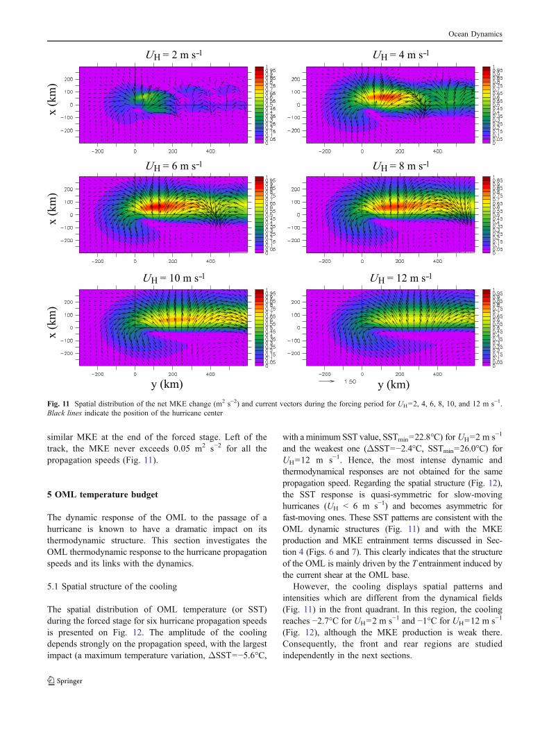
similar MKE at the end of the forced stage. Left of thetrack, the MKE never exceeds 0.05 m2 s−2 for all thepropagation speeds (Fig. 11).

5 OML temperature budget

The dynamic response of the OML to the passage of ahurricane is known to have a dramatic impact on itsthermodynamic structure. This section investigates theOML thermodynamic response to the hurricane propagationspeeds and its links with the dynamics.

5.1 Spatial structure of the cooling

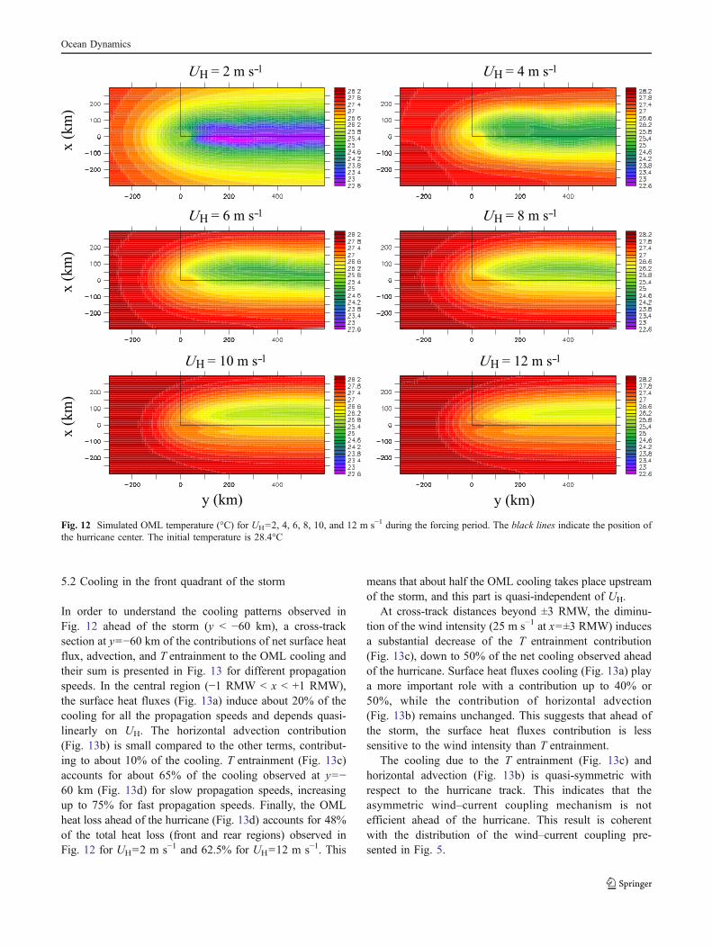
The spatial distribution of OML temperature (or SST)during the forced stage for six hurricane propagation speedsis presented on Fig. 12. The amplitude of the coolingdepends strongly on the propagation speed, with the largestimpact (a maximum temperature variation, ΔSST=−5.6°C,

with a minimum SST value, SSTmin=22.8°C) for UH=2 m s−1

and the weakest one (ΔSST=−2.4°C, SSTmin=26.0°C) forUH=12 m s−1. Hence, the most intense dynamic andthermodynamical responses are not obtained for the samepropagation speed. Regarding the spatial structure (Fig. 12),the SST response is quasi-symmetric for slow-movinghurricanes (UH < 6 m s−1) and becomes asymmetric forfast-moving ones. These SST patterns are consistent with theOML dynamic structures (Fig. 11) and with the MKEproduction and MKE entrainment terms discussed in Sec-tion 4 (Figs. 6 and 7). This clearly indicates that the structureof the OML is mainly driven by the T entrainment induced bythe current shear at the OML base.

However, the cooling displays spatial patterns andintensities which are different from the dynamical fields(Fig. 11) in the front quadrant. In this region, the coolingreaches −2.7°C for UH=2 m s−1 and −1°C for UH=12 m s−1

(Fig. 12), although the MKE production is weak there.Consequently, the front and rear regions are studiedindependently in the next sections.

Fig. 11 Spatial distribution of the net MKE change (m2 s−2) and current vectors during the forcing period for UH=2, 4, 6, 8, 10, and 12 m s−1.Black lines indicate the position of the hurricane center

Ocean Dynamics

5.2 Cooling in the front quadrant of the storm

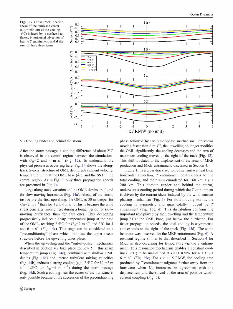
In order to understand the cooling patterns observed inFig. 12 ahead of the storm (y < −60 km), a cross-tracksection at y=−60 km of the contributions of net surface heatflux, advection, and T entrainment to the OML cooling andtheir sum is presented in Fig. 13 for different propagationspeeds. In the central region (−1 RMW < x < +1 RMW),the surface heat fluxes (Fig. 13a) induce about 20% of thecooling for all the propagation speeds and depends quasi-linearly on UH. The horizontal advection contribution(Fig. 13b) is small compared to the other terms, contribut-ing to about 10% of the cooling. T entrainment (Fig. 13c)accounts for about 65% of the cooling observed at y=−60 km (Fig. 13d) for slow propagation speeds, increasingup to 75% for fast propagation speeds. Finally, the OMLheat loss ahead of the hurricane (Fig. 13d) accounts for 48%of the total heat loss (front and rear regions) observed inFig. 12 for UH=2 m s−1 and 62.5% for UH=12 m s−1. This

means that about half the OML cooling takes place upstreamof the storm, and this part is quasi-independent of UH.

At cross-track distances beyond ±3 RMW, the diminu-tion of the wind intensity (25 m s−1 at x=±3 RMW) inducesa substantial decrease of the T entrainment contribution(Fig. 13c), down to 50% of the net cooling observed aheadof the hurricane. Surface heat fluxes cooling (Fig. 13a) playa more important role with a contribution up to 40% or50%, while the contribution of horizontal advection(Fig. 13b) remains unchanged. This suggests that ahead ofthe storm, the surface heat fluxes contribution is lesssensitive to the wind intensity than T entrainment.

The cooling due to the T entrainment (Fig. 13c) andhorizontal advection (Fig. 13b) is quasi-symmetric withrespect to the hurricane track. This indicates that theasymmetric wind–current coupling mechanism is notefficient ahead of the hurricane. This result is coherentwith the distribution of the wind–current coupling pre-sented in Fig. 5.

Fig. 12 Simulated OML temperature (°C) for UH=2, 4, 6, 8, 10, and 12 m s−1 during the forcing period. The black lines indicate the position ofthe hurricane center. The initial temperature is 28.4°C

Ocean Dynamics

5.3 Cooling under and behind the storm

After the storm passage, a cooling difference of about 2°Cis observed in the central region between the simulationswith UH=2 and 4 m s−1 (Fig. 12). To understand thephysical processes occurring here, Fig. 14 shows the along-track (y-axis) structure of OML depth, entrainment velocity,temperature jump at the OML base (δT), and the SST in thecentral region. As in Fig. 8, only three propagation speedsare presented in Fig. 14.

Large along-track variations of the OML depths are foundfor slow-moving hurricanes (Fig. 14a). Ahead of the storm,just before the first upwelling, the OML is 30 m deeper forUH=2 m s−1 than for 4 and 6 m s−1. This is because the windstress generates mixing here during a longer period for slow-moving hurricanes than for fast ones. This deepeningprogressively induces a sharp temperature jump at the baseof the OML, reaching 2.5°C for UH=2 m s−1 and 2°C for 4and 6 m s−1 (Fig. 14c). This stage can be considered as a“preconditioning” phase which modifies the upper oceanstructure before the upwelling takes place.

When the upwelling and the “out-of-phase” mechanismdescribed in Section 4.2 take place for low UH, this sharptemperature jump (Fig. 14c), combined with shallow OMLdepths (Fig. 14a) and intense turbulent mixing velocities(Fig. 14b), induces a strong cooling (e.g., 2.5°C for UH=2 ms−1; 1.5°C for UH=4 m s−1) during the storm passage(Fig. 14d). Such a cooling near the center of the hurricane isonly possible because of the succession of the preconditioning

phase followed by the out-of-phase mechanism. For stormsmoving faster than 6 m s−1, the upwelling no longer modifiesthe OML significantly, the cooling decreases and the area ofmaximum cooling moves to the right of the track (Fig. 12).This shift is related to the displacement of the areas of MKEproduction and MKE entrainment, discussed in Section 4.

Figure 15 is a cross-track section of net surface heat flux,horizontal advection, T entrainment contributions to thetotal cooling, and their sum cumulated for −60 km < y <200 km. This domain (under and behind the storm)underwent a cooling period during which the T entrainmentis driven by the current shear induced by the wind–currentphasing mechanism (Fig. 5). For slow-moving storms, thecooling is symmetric and quasi-totally induced by Tentrainment (Fig. 15c, d). This distribution confirms theimportant role played by the upwelling and the temperaturejump δT at the OML base, just below the hurricane. Forfaster propagation speeds, the total cooling is asymmetricand extends to the right of the track (Fig. 15d). The samebehavior was observed for the MKE entrainment (Fig. 6). Aresonant regime similar to that described in Section 4 forMKE is also occurring for temperature via the T entrain-ment. This resonance mechanism enables a constant cool-ing (−2°C) to be maintained at x=+1 RMW for 4 < UH <6 m s−1 (Fig. 15c). For x > +1.5 RMW, the cooling areaproduced by T entrainment migrates further away from thehurricane when UH increases, in agreement with thedisplacement and the spread of the area of positive wind–current coupling (Fig. 5).

Fig. 13 Cross-track sectionahead of the hurricane center(at y=−60 km) of the cooling(°C) induced by: a surface heatfluxes, b horizontal advection ofheat, c T entrainment, and d thesum of these three terms

Ocean Dynamics

Contrary to the upstream region, the contribution ofsurface heat fluxes (Fig. 15a) to the OML heat budget isvery weak compared to the T entrainment (Fig. 15c) underand behind the storm. The associated cooling is about −0.1°C,

which represents 5% to 10% of the total cooling. In thecentral region (−1 < x < +1 RMW), the minimum cooling(≈−0.05°C) is obtained for UH=2 m s−1 and the maximumcooling (≈−0.17°C) for UH=4 m s−1 to the left side of the

Fig. 15 Cross-track section ofthe cooling (°C) induced underand beneath the storm(for −60 km < y < 200 km) by: asurface heat flux, b horizontaladvection of heat, c Tentrainment, and d the sum ofthese three terms

Fig. 14 Along-track (y-axis, inkm) variations of a OML depth,h (m), b OML entrainmentvelocity, we (m s−1), c OMLtemperature jump, δT (°C),and d OML temperature (°C)

Ocean Dynamics

track. Globally, the contribution of surface heat fluxes isstronger on the left side. That can be explained by aweaker air–sea temperature difference on the right side.This cross-track difference results from the asymmetric Tentrainment. Consequently, the surface heat fluxes aredirectly connected to the intensity of the T entrainment.

The horizontal advection locally induces large warmingin the central region (−1 < x < +1 RMW; Fig. 15b).Intensities range from +1°C for UH=2 m s−1 to +0.1°C for12 m s−1. At greater distances from the center, the advectioncools the OML, with intensities ranging from −0.8°C for2 m s−1 to −0.1°C for 12 m s−1. Hence, the horizontaladvection of heat tends to attenuate the cold wake bytransporting warmer waters there. This process efficientlydecreases the cross-track temperature gradient.

Finally, it is important to note that the heat loss in theOML is not a linear function of the hurricane propagationspeed because the processes involved in the OML heatbudget are strongly nonlinear.

6 Conclusion

Idealized simulations of the OML response to hurricanesmoving with different propagation speeds were presented.We used a two-layer model based on the full primitiveequations, integrated over the OML depth. The entrainmentparameterization of Gaspar (1988) was modified in order totake into account the production of turbulence by currentshear. The model was validated by comparisons withobservations of Hurricane Frances (2004), which showedthat the simulated SSTs are in good agreement with thesatellite-derived values. The simulated dynamics of the coldwake compare quite well with the profiler data fromSanford et al. (2007). These results indicate that a simpleintegral model is able to simulate realistically the meancharacteristics of the OML response to a moving hurricane.The kinetic energy and heat budgets were derived from theintegration of the momentum and thermodynamic equationsduring the forced stage.

The non-dimensional storm speed S (Price 1983;Greatbatch 1984) is used to characterize the wind–currentcoupling and the OML response. The length scaleassociated with the wind field is based here on geometricconsiderations defined from the rotation angles of thewind and the current beneath the storm. We obtained anestimate of the ratio between the oceanic inertial and windrotation frequencies in the central region of the storm. Thehurricane propagation speed corresponding to the theoret-ical resonant regime (i.e., S=1) is UH=3 m s−1. The MKEbudget analysis has shown that the maximum MKEproduction during the forcing period is found at thepropagation speed of 4.5 m s−1 in the central region. This

value is slightly higher than the theoretical value deducedfrom S. The approximations made in the definition of theoceanic response frequency and of the atmospheric lengthscale can explain this difference.

The intensity and structure of the local coupling betweensurface wind and OML currents strongly depend on thehurricane propagation speed. This coupling modulates thewind stress energy flux at the air–sea interface by creatingtwo main zones of positive and negative energy transfer.These areas spread and move anticlockwise around thestorm center as UH increases. A similar behavior wasobserved in the earlier study of Chang and Anthes (1978).

The MKE production is found to be a strongly nonlinearfunction of the hurricane propagation speed with differentlocal maxima depending on the cross-track distance. A localresonant regime is deduced from the MKE productionanalysis. Considering that the hurricane wind profile imposesa decrease of the wind rotation frequency with the distance tothe storm center, the propagation speed defines the cross-trackposition of the local resonant regime.

About 60% of the MKE injected in the OML isdissipated. This ratio (dissipation over MKE injection)remains quasi-constant for UH > 6 m s−1, suggesting thatthe MKE entrainment adjusts to the propagation speed.Consequently, the MKE production is quasi-balanced bythe MKE entrainment for fast-moving hurricanes so that theMKE at the end of the forcing period is roughly constant.

For slow-moving hurricanes (<6 m s−1), MKE entrain-ment and vertical turbulent mixing increase dramatically inthe central region due to the influence of the upwellingwhich occurs in the MKE entrainment zone (Price 1981). Adetailed analysis shows that for slow-moving hurricanes,upwelling and entrainment velocities are out of phasebefore the second wind peak. This mechanism increases theMKE entrainment up to 40% in the central regioncompared to the case without upwelling. Finally, theMKE storage is very weak for slow-moving hurricanesbecause upwelling strongly enhances MKE entrainment inthe region of maximum MKE production. Similar behaviorwas observed by Chang and Anthes (1978) in terms ofcurrent intensity when a storm moves slowly. For fasterhurricanes, the shift between upwelling and entrainment istoo important and a resonant regime can be set up on theright side of the track where a zone of maximum MKEproduction occurs.

In the MKE budget, the contributions of horizontaladvection and pressure gradient terms are small compared tothe other terms. Horizontal advection exports energy outsidethe central region whatever the propagation speed. Thepressure term tends to trap MKE in the central region forslow-moving hurricanes and to export MKE out of the centralregion for faster hurricanes. This behavior is induced by cross-track variations of the OML depth, which is shallower in the

Ocean Dynamics

central region due to upwelling. Advection is broadlybalanced by the pressure term for slow-moving hurricanes.For faster hurricanes, both terms are weak.

The heat budget is strongly affected by the surface windsahead of the hurricane. About 50% of the total heat loss occursupstream independently of UH. This cooling is not related tothe wind–current coupling mechanism which is negligibleahead of the storm. This can be seen as a “preconditioning”phase of the OML during which the temperature jumpthrough the thermocline increases for slow-moving hurri-canes. When the upwelling is set up in the central region, itstrongly enhances the entrainment because of the strongentrainment velocity and large temperature jump at the top ofthe thermocline. This mechanism is associated with the “out-of-phase” mechanism described previously. In the centralregion, it contributes to increase the total OML cooling bynearly 80% for UH=2 m s−1 and 50% for UH=4 m s−1

compared to the case without upwelling and with a fixedtemperature jump. These results are in agreement withGreatbatch (1983) who observed that the OML coolingincreases by a factor 2 for UH=2.5 m s−1 and with Price(1981) who found that the cooling increases by 35% forUH=4 m s−1 when the upwelling is taken into account. For

fast-moving hurricanes, the OML temperature response isdirectly driven by the local resonant regime which explainsthe shift of the cold wake to the right of the track. Surfaceheat fluxes have a negligible contribution (5–10%) to theheat budget beneath and after the storm. Horizontaladvection redistributes the heat content by carrying warmerwater into the cold wake.

These results highlight the role of the hurricanepropagation speed on the OML dynamics and thermody-namics. For slow-moving storms, the OML structure issensitive to the propagation speed which sets up thesequence of central upwelling and entrainment velocitynear the central part of the storm. In this regime, smallvariations of the propagation speed can induce largevariations in the OML currents and temperature. Theresults obtained for Hurricane Frances (2004) illustratethis point quite well. With a 6-h time resolution, thevariations of the hurricane propagation speed are wellresolved and allow to properly simulate the strongestcooling. Finally, this study highlights the necessity toconsider the propagation speed as a key parameter toaccurately describe and understand the oceanic responseto a moving hurricane.

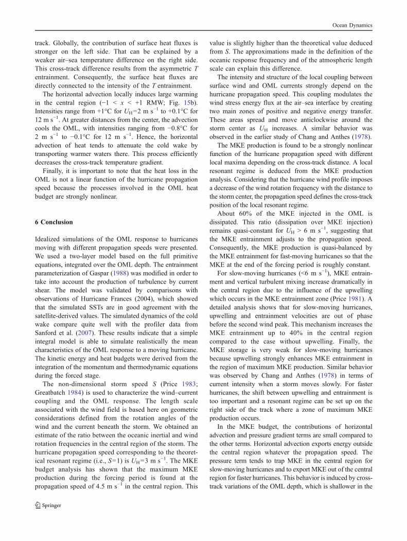
Fig. 16 Symmetric andasymmetric surface wind fields(m s−1) with 10-m s−1

isocontours

Ocean Dynamics

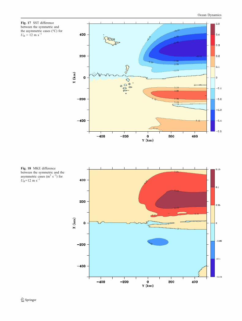
Fig. 17 SST differencebetween the symmetric andthe asymmetric cases (°C) forUH = 12 m s−1

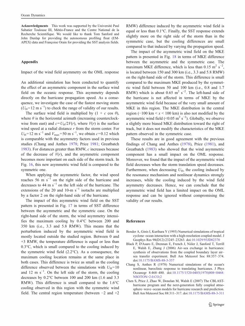
Fig. 18 MKE differencebetween the symmetric and theasymmetric cases (m2 s−2) forUH=12 m s−1

Ocean Dynamics

Acknowledgments This work was supported by the Université PaulSabatier Toulouse III, Météo-France and the Centre National de laRecherche Scientifique. We would like to thank Tom Sanford andJohn Dunlap for providing the autonomous profiling float (EM-APEX) data and Françoise Orain for providing the SST analysis fields.

Appendix

Impact of the wind field asymmetry on the OML response

An additional simulation has been conducted to quantifythe effect of an asymmetric component in the surface windfield on the oceanic response. This asymmetry dependsdirectly on the hurricane propagation speed. As a conse-quence, we investigate the case of the fastest moving storm(UH=12 m s−1) to check the range of validity of our results.

The surface wind field is multiplied by (1 + c cos θ),where θ is the horizontal azimuth (increasing counterclock-wise from east) and c=UH/2V(r), where V(r) is the surfacewind speed at a radial distance r from the storm center. ForUH=12 m s−1 and Vmax=50 m s−1, we obtain c=0.12 whichis comparable with the asymmetry factors used in previousstudies (Chang and Anthes 1978; Price 1981; Greatbatch1983). For distances greater than RMW, c increases becauseof the decrease of V(r), and the asymmetric componentbecomes more important on each side of the storm track. InFig. 16, this new asymmetric wind field is compared to thesymmetric one.

When applying the asymmetric factor, the wind speedreaches 56 m s−1 on the right side of the hurricane anddecreases to 44 m s−1 on the left side of the hurricane. Theextensions of the 20 and 10-m s−1 isotachs are multipliedby a factor 2 on the right-hand side of the hurricane.

The impact of this asymmetric wind field on the SSTpattern is presented in Fig. 17 in terms of SST differencebetween the asymmetric and the symmetric case. On theright-hand side of the storm, the wind asymmetry intensi-fies the maximum cooling by 0.4°C between 200 and350 km (i.e., 3.3 and 5.8 RMW). This means that theperturbation induced by the asymmetric wind field ismostly located outside the studied region. Between 0 and+3 RMW, the temperature difference is equal or less than0.3°C, which is small compared to the cooling induced bythe symmetric wind field (2.2°C). As a consequence, themaximum cooling location remains at the same place inboth cases. This difference is twice as small as the coolingdifference observed between the simulations with UH=10and 12 m s−1. On the left side of the storm, the coolingdecreases by 0.2°C between 100 and 200 km (1.6 and 3.3RMW). This difference is small compared to the 1.6°Ccooling observed in this region with the symmetric windfield. The central region temperature (between −2 and +2

RMW) difference induced by the asymmetric wind field isequal or less than 0.1°C. Finally, the SST response extendsslightly more on the right side of the storm than in thesymmetric case, but the cooling differences are smallcompared to that induced by varying the propagation speed.

The impact of the asymmetric wind field on the MKEpattern is presented in Fig. 18 in terms of MKE differencebetween the asymmetric and the symmetric case. Themaximum MKE difference, which is less than 0.15 m2 s−2,is located between 150 and 300 km (i.e., 3.3 and 5.8 RMW)on the right-hand side of the storm. This difference is smallcompared to the maximum MKE produced by the symmet-ric wind field between 50 and 100 km (i.e., 0.8 and 1.7RMW) which is about 0.65 m2 s−2. The left-hand side ofthe hurricane is not affected in terms of MKE by theasymmetric wind field because of the very small amount ofMKE in this region. The MKE distribution in the centralregion (−100 km < x < 100 km) is also not modified by theasymmetric wind field (<0.05 m2 s−2). Globally, we observea slightly more biased MKE distribution toward the right oftrack, but it does not modify the characteristics of the MKEpattern observed in the symmetric case.

These results are in good agreement with the previousfindings of Chang and Anthes (1978), Price (1981), andGreatbatch (1983) who showed that the wind asymmetriccomponent has a small impact on the OML response.Moreover, we found that the impact of the asymmetric windfield decreases when the storm translation speed decreases.Furthermore, when decreasing UH, the cooling induced bythe resonance mechanism and nonlinear dynamics stronglyincreases, while the cooling induced by the wind fieldasymmetry decreases. Hence, we can conclude that theasymmetric wind field has a limited impact on the OMLresponse and can be ignored without compromising thevalidity of our results.

References

Bender A, Ginis I, Kurihara Y (1993) Numerical simulations of tropicalcyclone–ocean interaction with a high-resolution coupled model. JGeophys Res 98(D12):23245–23263. doi:10.1029/93JD02370

Black P, D'Asaro E, Drennan E, French J, Niiler J, Sanford T, TerrillE, Walsh E, Zhang J (2006) Air–sea exchange in hurricanes:synthesis of observations from the coupled boundary layer air–sea transfer experiment. Bull Am Meteorol Soc 88:357–374.doi:10.1175/BAMS-88-3-357

Chang S, Anthes R (1978) Numerical simulations of the ocean'snonlinear, baroclinic response to translating hurricanes. J PhysOceanogr 8:468–480. doi:10.1175/1520-0485(1978)008<0468:NSOTON>2.0.CO;2

Chen S, Price J, Zhao W, Donelan M, Walsh E (2007) The CBLAST-hurricane program and the next-generation fully coupled atmo-sphere–wave–ocean models for hurricane research and prediction.Bull AmMeteorol Soc 88:311–317. doi:10.1175/BAMS-88-3-311

Ocean Dynamics

D'Asaro E, Sanford T, Niiler P, Terrill E (2007) Cold wake ofHurricane Frances. Geophys Res Lett 34:15. doi:10.1029/2007GL030160

Donelan M, Haus B, Reul N, Plant W, Stiassnie M, Graber H, BrownO, Saltzman E (2004) On the limiting aerodynamic roughness ofthe ocean in very strong winds. Geophys Res Lett 31:18.doi:10.1029/2004GL019460

Donlon C, Robinson I, Casey KS, Vazquez-Cuervo J, ArmstrongE, Arino O, Gentemann C, May D, LeBorgne P, Piollé J,Barton I, Beggs H, Poulter DJS, Merchant CJ, Bingham A,Heinz S, Harris A, Wick G, Emery B, Minnett P, Evans R,Llewellyn-Jones D, Mutlow C, Reynolds RW, Kawamura H,Rayner N (2007) The global ocean data assimilation experi-ment high-resolution sea surface temperature pilot project.Bull Am Meteorol Soc 88:1197–1213. doi:10.1175/BAMS-88-8-1197

Drennan W, Zhang J, French J, McCormick C, Black P (2007)Turbulent fluxes in the hurricane boundary layer. Part II: latentheat flux. J Atmos Sci 64(4):1103–1115. doi:10.1175/JAS3889.1

Emanuel K (1986) An air–sea interaction theory for tropical cyclones.Part I. Steady-state maintenance. J Atmos Sci 43(6):585–605.doi:10.1175/1520-0469(1986)043<0585:AASITF>2.0.CO;2

Emanuel K (1995) Sensitivity of tropical cyclones to surface exchangecoefficients and a revised steady-state model incorporating eyedynamics. J Atmos Sci 52(22):3969–3976. doi:10.1175/1520-0469(1995)052<3969:SOTCTS>2.0.CO;2

Emanuel K (2003) A similarity hypothesis for air–sea exchange atextreme wind speeds. J Atmos Sci 60(11):1420–1428

French J, Drennan W, Zhang J, Black P (2007) Turbulent fluxes in thehurricane boundary layer. Part I: momentum flux. J Atmos Sci 64(4):1089–1102. doi:10.1175/JAS3887.1

Garwood R Jr (1977) An oceanic mixed layer model capable ofsimulating cyclic states. J Phys Oceanogr 7(3):455–468.doi:10.1175/1520-0485(1977)007<0455:AOMLMC>2.0.CO;2

Gaspar P (1988) Modeling the seasonal cycle of the upper ocean. JPhys Oceanogr 18(2):161–180. doi:10.1175/1520-0485(1988)018<0161:MTSCOT>2.0.CO;2

Geisler J (1970) Linear theory of the response of a two layer ocean toa moving hurricane. Geophys Astrophys Fluid Dyn 1:249–272

Gill AE (1984) On the behavior of internal waves in the wakes ofstorms. J Phys Oceanogr 14(7):1129–1151. doi:10.1175/1520-0485(1984)014<1129:OTBOIW>2.0.CO;2

Greatbatch R (1983) On the response of the ocean to a moving storm:the nonlinear dynamics. J Phys Oceanogr 13(3):357–367.doi:10.1175/1520-0485(1983)013<0357:OTROTO>2.0.CO;2

Greatbatch R (1984) On the response of the ocean to a moving stormparameters and scales. J Phys Oceanogr 14(1):59–78.doi:10.1175/1520-0485(1984)014<0059:OTROTO>2.0.CO;2

Holland G (1980) Analytic model wind press profiles hurricanes. MonWeather Rev 108(8):1212–1218

Jacob S, Shay L (2003) The role of oceanic mesoscale features on thetropical cyclone-induced mixed layer response. A case study. JPhys Oceanogr 33(4):649–676. doi:10.1175/1520-0485(2003)33<649:TROOMF>2.0.CO;2

Kolmogorov AN (1942) The equation of turbulent motion in anincompressible fluid. Izv Akad Nauk SSSR Ser Fiz 6:56–58

Kraus EB, Turner JS (1967) A one-dimensional model of the seasonalthermocline. II. The general theory and its consequences. Tellus19:98–106

Levitus S, Boyer TP (1994) World Ocean Atlas 1994, vol 4.Temperature. NOAA Atlas NESDIS 4. US Government PrintingOffice, Washington, DC, 117 pp

Levitus S, Burgett R, Boyer TP (1994) World Ocean Atlas 1994, vol3. Salinity. NOAA Atlas NESDIS 3. US Government PrintingOffice, Washington, DC, 99 pp

Makin V (2005) A note on the drag of the sea surface at hurricanewinds bound-layer. Meteorology 115(1):169–176

Niiler P, Kraus E (1977) One dimension models of the upper ocean.In: Kraus EB (ed) Modeling and prediction of upper layers of theocean. Pergamon, New York, pp 143–172

O’Brien JJ (1967) The non-linear response of a two-layer, baroclinicocean to a stationary, axially-symmetric hurricane. Part II.Upwelling induced by momentum transfer. J Atmos Sci 24(2):208–214

Powell M, Houston S, Amat L, Morisseau-Leroy N (1998) The HRDreal-time hurricane wind analysis system. J Wind Eng IndAerodyn 77:53–64

Powell M, Vickery P, Reinhold T (2003) Reduced drag coefficient forhigh wind speeds in tropical cyclones. Nature 422:279–283.doi:10.1038/nature01481

Price J (1981) Upper ocean response to a hurricane. J Phys Oceanogr11(2):153–175. doi:10.1175/1520-0485(1981)011<0153:UORTAH>2.0.CO;2

Price J (1983) Internal wave wake of a moving storm. Part I: scales,energy budget and observations. J Phys Oceanogr 13(6):949–965.doi:10.1175/1520-0485(1981)011<0153:UORTAH>2.0.CO;2

Price J, Sanford T, Forristall G (1994) Forced stage response to amoving hurricane. J Phys Oceanogr 24(2):233–260. doi:10.1175/1520-0485(1994)024<0233:FSRTAM>2.0.CO;2

Sanford T, Black P, Haustein J, Feeney J, Forristall G, Price J (1987)Ocean response to a hurricane. Part I: observations. J Phys Oceanogr17(11):2065–2083. doi:10.1175/1520-0485(1987)017<2065:ORTAHP>2.0.CO;2

Sanford T, Price J, Girton J,Webb D (2007) Highly resolved observationsand simulations of the ocean response to a hurricane. Geophys ResLett 34(13):L13604. doi:10.1029/2007GL029679

Schade L (2000) Tropical cyclone intensity and sea surface temper-ature. J Atmos Sci 57(18):3122–3130

Shay L, Elsberry R, Black P (1989) Vertical structure of the oceancurrent response to a hurricane. J Phys Oceanogr 19(5):649–669.doi:10.1175/1520-0485(1989)019<0649:VSOTOC>2.0.CO;2

Shay L, Black P, Mariano A, Hawkins J, Elsberry R (1992) Upperocean response to Hurricane Gilbert. J Geophys Res 97(C12):20227–20248. doi:10.1029/92JC01586

Weill A, Eymard L, Caniaux G, Hauser D, Planton S, Dupuis H, Brut A,Guerin C, Nacass P, Butet A et al (2003) Toward a betterdetermination of turbulent air–sea fluxes from several experiments.J Clim 16(4):600–618

Ocean Dynamics