Physical and Bio-optical Observations of Oceanic Cyclones West of the Island of Hawai’i Tommy D. Dickey a,* Francesco Nencioli a Victor S. Kuwahara a,b Carrie Leonard c Wil Black a Yoshimi M. Rii d Robert R. Bidigare d Qin Zhang a a Ocean Physics Laboratory, Department of Geography, University of California Santa Barbara, Goleta, CA, USA b Currently at Faculty of Education, Soka University, Tokyo, Japan c BAE Systems, Honolulu, HI, USA d SOEST, Department of Oceanography, University of Hawai’i, Manoa, HI, USA Abstract Interdisciplinary observations of mesoscale eddies were made to the west of the is- land of Hawaii. A central goal of the studies was to improve our understanding of the coupling of physical, biological, and biogeochemical processes that occur within these eddies. A specific objective was to test the hypothesis that the physical mech- anisms of mesoscale eddies result in increases in nutrient availability to the euphotic layer, increases in primary production, changes in biological community composi- tions and size distributions, and increases in carbon flux to the deep sea. Data were obtained from ships, surface drifters, and satellite sensors during three separate field experiments. Variability was associated with two well-developed cyclonic, cold-core mesoscale eddies, Cyclone Noah and Cyclone Opal, which were observed during the E-Flux I (survey November 6-20, 2004) and E-Flux III (survey March 10-27, 2005) field campaigns, respectively. No mesoscale eddies were found during E-Flux II (survey January 10-19) when winds were erratic in magnitude and direction, sup- porting the hypothesis that persistent trade winds drive the production of cold-core mesoscale eddies in the lee of the Hawaiian Islands. Cold-core eddies were present in the E-Flux study area for about 2/3 of a year beginning May 1, 2004 and trade winds prevailed for about 3/4 of the same year. Both Cyclone Noah and Cyclone Opal were generated during strong, persistent northeasterly trade wind conditions and appeared downwind of the ’Alenuihaha Channel separating the islands of Maui and Hawai’i. The likely production mecha- nism for both mesoscale cold-core eddies involves localized wind stress curl-induced upwelling produced by trade wind forcing. Cyclone Noah was likely spun up by strong trade winds just to the southwest of the ’Alenuihaha Channel (∼20.10 ◦ N, 156.40 ◦ W) between August 13 and 21, 2004 based on MODIS satellite sea surface Preprint submitted to Elsevier 30 July 2007

Welcome message from author
This document is posted to help you gain knowledge. Please leave a comment to let me know what you think about it! Share it to your friends and learn new things together.
Transcript

Physical and Bio-optical Observations of
Oceanic Cyclones West of the Island of
Hawai’i
Tommy D. Dickey a,∗ Francesco Nencioli a
Victor S. Kuwahara a,b Carrie Leonard c Wil Black a
Yoshimi M. Rii d Robert R. Bidigare d Qin Zhang a
aOcean Physics Laboratory, Department of Geography, University of CaliforniaSanta Barbara, Goleta, CA, USA
bCurrently at Faculty of Education, Soka University, Tokyo, JapancBAE Systems, Honolulu, HI, USA
dSOEST, Department of Oceanography, University of Hawai’i, Manoa, HI, USA
Abstract
Interdisciplinary observations of mesoscale eddies were made to the west of the is-land of Hawaii. A central goal of the studies was to improve our understanding ofthe coupling of physical, biological, and biogeochemical processes that occur withinthese eddies. A specific objective was to test the hypothesis that the physical mech-anisms of mesoscale eddies result in increases in nutrient availability to the euphoticlayer, increases in primary production, changes in biological community composi-tions and size distributions, and increases in carbon flux to the deep sea. Data wereobtained from ships, surface drifters, and satellite sensors during three separate fieldexperiments. Variability was associated with two well-developed cyclonic, cold-coremesoscale eddies, Cyclone Noah and Cyclone Opal, which were observed duringthe E-Flux I (survey November 6-20, 2004) and E-Flux III (survey March 10-27,2005) field campaigns, respectively. No mesoscale eddies were found during E-FluxII (survey January 10-19) when winds were erratic in magnitude and direction, sup-porting the hypothesis that persistent trade winds drive the production of cold-coremesoscale eddies in the lee of the Hawaiian Islands. Cold-core eddies were presentin the E-Flux study area for about 2/3 of a year beginning May 1, 2004 and tradewinds prevailed for about 3/4 of the same year.
Both Cyclone Noah and Cyclone Opal were generated during strong, persistentnortheasterly trade wind conditions and appeared downwind of the ’AlenuihahaChannel separating the islands of Maui and Hawai’i. The likely production mecha-nism for both mesoscale cold-core eddies involves localized wind stress curl-inducedupwelling produced by trade wind forcing. Cyclone Noah was likely spun up bystrong trade winds just to the southwest of the ’Alenuihaha Channel (∼20.10N,156.40W) between August 13 and 21, 2004 based on MODIS satellite sea surface
Preprint submitted to Elsevier 30 July 2007

temperature (SST) imagery and QuikScat satellite wind data, and apparently be-gan to dissipate by mid-December 2004. Cyclone Opal was likely spun up by strongtrade winds between February 2 and 18, 2005 southwest of the ’Alenuihaha Channel(∼20.30N, 156.30W), but was no longer evident in April 2005.
Both Cyclone Noah and Cyclone Opal had strong physical, chemical, and biologi-cal expressions and displayed similar maximum tangential current speeds of ∼60 cmsec−1. However, Cyclone Opal was more symmetric and larger in scale (roughly 180− 200 km in diameter compared to ∼160 km in horizontal scale for Cyclone Noah).Both mesoscale eddies displayed significant doming in their centers and in somecases outcroppings of isothermal, isopycnal, nutrient, and chlorophyll a isopleths.After formation and a slow drift southward, Cyclone Noah remained in nearly thesame location (roughly 19.60N, 156.50W) during the 3-week in situ sampling pe-riod, whereas Cyclone Opal drifted southward by ∼165 km over a similar time spanof sampling. Interestingly, the physical manifestations of both features were rela-tively unchanged during the ship-based surveys; however, the biology appears tohave evolved within Cyclone Opal. The present report sets the context for severalother E-Flux studies.
Key words: Hawai’i, Mesoscale processes, Cyclonic eddies, E-FLUX project,Physical-biological coupling
1 Introduction
Mesoscale eddies are generally thought to play important roles in oceancirculation, heat and mass transport, mixing, biological productivity, up-per ocean ecology, fisheries, and biogeochemistry including elemental cyclingand fluxes ( e.g., Cheney and Richardson, 1976; Olson, 1980; Lobel andRobinson, 1986; Falkowski et al., 1991; Dickey et al., 1993; Allen et al.,1996; McGillicuddy and Robinson, 1997; McGillicuddy et al., 1998; Oschliesand Garcon, 1998; Honjo et al., 1999; McNeil et al., 1999; Letelier et al.,2000; Fischer et al., 2002; Garcon et al., 2001; Leonard et al., 2001; Oschlies,2001; Seki et al., 2001, 2002; Flierl and McGillicuddy, 2002; Lewis, 2007; Bidi-gare et al., 2003; Taupier-Letage et al., 2003; Sakamoto et al., 2004). Thehorizontal dimensions of mid-latitude mesoscale eddy features generally rangefrom about 100 to 250 km in diameter with scaling roughly dictated by theRossby radius of deformation (e.g., Richman et al., 1977). Fully developededdies are often in near geostrophic balance although the ageostrophic compo-nent can be important. A variety of physical processes have been hypothesizedto contribute to mesoscale eddy formation. For example, eddies or rings in the
∗ Corresponding author. Tel.: +1-805-893-7354; fax: +1-805-967-5704.Email address: [email protected] (Tommy D. Dickey).
2

vicinity of western boundary currents like the Gulf Stream and the Kuroshiomay be generated through inertial instabilities, open ocean eddies may be pro-duced through baroclinic instabilities, and eddies formed in the vicinity of seamounts may be caused by barotropic instabilities.
Islands can clearly perturb ocean circulation patterns as well documented forthe Hawaiian Island chain (e.g., Qiu et al., 1997; Lumpkin, 1998). Further,mesoscale eddies are also often evident near islands as indicated by the obser-vations reported here and elsewhere (e.g., Patzert, 1969; Barton, 2001; Lump-kin, 1998). It has been suggested that instabilities associated with currentflow past islands or through island passages can generate eddies (e.g., Aris-tegui et al., 1994, 1997; Barton et al., 2000, 2001). Another mechanism forgenerating eddies involves the acceleration of winds through island channelswith high mountains on either side. Gradients in the wind fields on the leesides of such islands can produce wind stress curl distributions that result in lo-calized oceanic upwelling and downwelling and both warm-core and cold-coremesoscale eddies. The latter mechanism appears to explain the productionof eddies in the lee of the Hawaiian Islands based on the results of previousinvestigators and our current study (e.g., Patzert, 1969; Lumpkin, 1998; Hol-land and Mitchum, 2001; Chavanne et al., 2002). It is worth emphasizingthat warm-core anti-cyclonic eddies are also produced via the wind stress curlmechanism as well as by a shear instability mechanism by drawing energyfrom the North Equatorial Current as it impinges on Hawaii and separates atthe southern tip of the island (Lumpkin, 1998). As noted by an anonymousreviewer, these warm-core eddies may interact with adjacent cold-core eddiesand act to suppress biological productivity where they originate and propa-gate. Our focus here is principally on cold-core eddies, which were sampleddirectly during our studies. Interaction among eddies is considered in otherE-Flux papers.
The central goal of the E-Flux experiment was to improve our fundamentalunderstanding of the coupling of physical, biological, and biogeochemical pro-cesses that occur within mesoscale eddies. Importantly, some researchers havesuggested that mesoscale eddies are major contributors of carbon to the deepsea (e.g., McGillicuddy et al., 1998) while others argue that they may haveless of an impact than suggested by McGillicuddy et al. (1998), (e.g., Oschliesand Garcon, 1998). This controversy bears directly on establishing the rolesand modeling of mesoscale features as they may affect elemental budgets,fluxes, and the ecology of the upper ocean. More specifically, the effects ofsuch features on nutrient availability, primary production, biological commu-nity structures and size distributions, and fluxes of elements including carbonand silicon to the deep sea remain contentious.
The recurrent nature of eddies to the west of the Hawaiian Islands during per-sistent trade wind conditions was a primary stimulus for the present E-Flux
3

experiment. In particular, it has been previously reported that westward prop-agating cyclonic eddies are produced in the lee of the Hawaiian Islands on timescales of 50 − 70 days ( Lumpkin, 1998; Seki et al., 2002). Previous studies inthe lee of the Hawaiian Islands and North Pacific environs have demonstratedthat cold-core mesoscale eddies play significant roles in the region’s biogeo-chemistry, biology, and fisheries (e.g., Lobel and Robinson, 1986; Falkowskiet al., 1991; Leonard et al., 2001; Seki et al., 2001, 2002; Bidigare et al.,2003; Vaillancourt et al., 2003). Thus, E-Flux investigators conducted a se-ries of three dedicated field experiments to address the various biogeochemicalmechanisms hypothesized to lead to enhanced carbon export. This paper re-views the general background of each of the three separate field experiments,the sampling strategies and methods employed, and general observational re-sults with emphases on physical and bio-optical aspects.
2 Observational Site, Objectives, and Methods
2.1 Site
Although mesoscale eddies are rather ubiquitous in the ocean, they remaindifficult to study in sufficient detail because they are generally ephemeral andevolve too quickly in geographically diverse locations to be easily sampledusing present-day observational tools (e.g., Bidigare et al., 2003; Dickey andBidigare, 2005). With these constraints in mind, the site for the E-Flux fieldexperiments, to the west of the southeastern Hawaiian Islands of Maui andHawai’i, was chosen on the basis of several criteria. First, it was deemed im-portant to choose a region where mesoscale eddies regularly form. Historicalhydrographic and satellite data sets (e.g., Patzert, 1969; Lumpkin, 1998; Cha-vanne et al., 2002; Seki et al., 2001, 2002; Bidigare et al., 2003) indicated thatmesoscale eddies typically develop and persist for weeks to several months tothe west of the Hawaiian Island chain during persistent trade wind conditions(winds generally from the northeast). In addition, previous studies in this por-tion of the ocean have indicated that regional cyclonic eddies have significantbiological and biogeochemical signatures (i.e., Seki et al., 2001, 2002; Bidigareet al., 2003; Vaillancourt et al., 2003). From a practical standpoint, it was alsodesirable to conduct our field experiments in a region which was readily acces-sible from a major port to minimize ship transit times and thus to maximizeship sampling capabilities. Moreover, the observations needed to be conductedin deep oceanic waters that were relatively uninfluenced by coastal processes(i.e., coastal upwelling, jets, and filaments as well as rain runoff) so that theresults would have general applicability to open ocean settings. All of thesecriteria were met by the region to the west of the islands of Maui and Hawai’i.The three E-Flux field experiments, which lasted approximately three weeks
4

each, spanned the period of November 4, 2004 to March 28, 2005; specifically,E-Flux I November 4 − 22, 2004; E-Flux II January 10 − 28, 2005; and E-Flux III March 10 − 28, 2005. The periods selected for the experiment werebased on wind climatology, essentially optimizing the chances for strong andpersistent trade winds. It is worth noting that a multi-platform approach wasused to optimally sample mesoscale features with the best possible temporaland spatial resolution under the budgetary and logistical constraints of theproject. Thus, satellites, ships, and drifters were utilized in the collection ofour data sets.
2.2 Observational Objective and Methods
The primary observational objective for the three E-Flux field experiments wasto obtain interdisciplinary data to enable the location, characterization, andinterpretation of the physical, optical, biogeochemical, and biological struc-tures and dynamics of mesoscale eddy features off Maui and Hawai’i. The R/VKa’imikai-O-Kanaloa (KOK ) was used for the E-Flux I experiment and theR/V Wecoma was used for the E-Flux II and III cruises. The methods used forthe physical, bio-optical, and chemical measurements during the three E-Fluxfield experiments were quite similar although some instrumentation differedbetween the two research vessels. For convenience, the general methodologiesused for the three experiments are presented within the following subgroups:1) ship-based profile measurements, 2) ship-based acoustic Doppler currentprofile (ADCP) measurements, 3) drifter measurements, 4) satellite measure-ments, and 5) an overview of measurements.
(1) Ship-based Profile Measurements : During the E-Flux cruises, mea-surements were made with profiled CTD/rosette packages at sta-tions deemed to be very near the centers of mesoscale eddy features(called IN stations), along several intersecting horizontal transects thatwere selected to pass through the best-estimated centers of the ed-dies, and well outside of them (called OUT stations). The CTD sys-tems were used to measure temperature, conductivity, pressure, chloro-phyll a fluorescence, beam transmission (660nm) or light backscatter-ing (for inferring particle concentrations and distributions), photosyn-thetic available radiation/scalar irradiance (PAR), and dissolved oxy-gen. Details concerning specific sensors may be found on University ofHawai’i SOEST (R/V KOK ) and Oregon State University (R/V We-coma) websites (http://www.soest.hawaii.edu/HURL/KOK specs.html,http://www.shipsops.oregonstate.edu/ops/wecoma/). During E-Flux I,a 24-bottle, 12-liter rosette was used to collect water samples, whereasa 12-bottle rosette sampler equipped with 10-liter bottles was used forE-Flux II and III operations. Multiple profiles were generally made to
5

depths of approximately 500, 1000, or 3000 m. Rosette bottles weretripped at multiple depths, which were selected on the basis of the ver-tical structure of the physical, optical, chemical, and biological variables(i.e., in the mixed layer, at the depth of a selected isopycnal surface,within the euphotic zone, and in the deep chlorophyll maximum re-gion). The CTD sensors were calibrated after each cruises (bottle sam-ples were not used for salinity calibration). The sampling rate of theCTDs (SBE 9/11+ units) was 24 Hz and most profiles were done witha vertical profiling rate of 0.50 m sec−1. Data were recorded duringboth up- and downcasts. The SBE Data Processing software suite wasused to convert the raw binary data into engineering units. Manufac-turer’s configuration files were used in the process. The same softwarewas used to further process the data following the procedures describedin the SBE Data Processing User Manual (http://www.seabird.com/-pdf documents/manuals/SBEDataProcessing 7.10.pdf).
A low-pass filter (default time constant of 0.15 sec) was applied tothe pressure record in order to smooth out high frequency data (seeSea-Bird SBE Data Processing User Manual for details). An alignmentprocedure was also applied to account for the different positions ofthe sensors on the rosette and their respective response times. CTDdata collected during excessive ship roll were eliminated, thus remov-ing the bins recorded when the vertical profile velocity was less than0.15 m sec−1. Data were then averaged into 1 m (1 db) bins andsalinity and density were derived from temperature, conductivity andpressure measurements following the UNESCO equations (UNESCO,1981). More information concerning the CTD data processing proce-dure can be found on the Sea-Bird website given above and an OPLData Report (http://orca.opl.ucsb.edu:8080/plone/eflux/eflux3/casts/-Data Processing v1.3.pdf). After processing, the CTD data were alsoquality controlled by comparing CTD values with climatological data forthe experimental region. Data values that were different by more than2 standard deviations (i.e., outliers) from the climatological mean wereeliminated.
Samples for nitrate+nitrite (µM l−1) and chlorophyll a (mg m−3) werecollected at discrete depths using the rosette sampler (see Rii et al., thisvolume). Nitrate+nitrite samples were analyzed in the laboratory usinga Technicon Autoanalyzer II. For determinations of chlorophyll a, 2-lwater samples were filtered immediately after collection and analyzed(post-cruise) using high performance liquid chromatography. These dis-crete values of total chlorophyll concentration were used to determinethe total chlorophyll-fluorescence regression coefficients for the E-Flux Iand E-Flux III cruises. These coefficients were then used to convert flu-orescence voltage into total chlorophyll a concentrations. Unfortunately,for the E-Flux II cruise it was not possible to compute the regressioncoefficients, because HPLC measurements on the collected water samples
6

were not available; therefore the conversion was made using the same co-efficients computed for the E-Flux III cruise (same fluorometer). The 1%light level depths were directly computed from scalar irradiance (PAR)profiles for the CTD casts collected during daytime. These data wereused to compute the relationship between the 1% light level depths andthe mean total chlorophyll concentrations between the surface and the1% light level depths. The coefficients were then used to derive the 1%light levels depths for the casts collected at night from total chlorophylla concentration data (Morel, 1988). Unfortunately, no discrete dissolvedoxygen data were obtained from the water samples, and thus it was notpossible to properly post-calibrate the dissolved oxygen sensor. Hence, itis not possible to verify the accuracy of oxygen concentrations. Nonethe-less, individual profiles can still be compared within a specific cruise,but it is not possible to compare absolute oxygen concentration valuesbetween cruises.
For some profile measurements, a specialized optics package was teth-ered 1.5 m beneath the CTD/rosette. The optics package was equippedwith two spectral absorption-attenuation instruments (WETLabs AC-9and AC-S), a fluorometer/turbidity instrument (WETLabs FLNTU),and a Sea-Bird CTD. Also, both ships collected meteorological and nearsurface (flow-through) physical, chemical, and biological data. Neitherthe optics package data nor the ship underway data are discussed in thepresent report.
(2) Ship-based ADCP Data: The simultaneous mapping of upper ocean cur-rents as functions of depth and geographic position was a critical partof the E-Flux experiment. ADCP data were used not only to determinethe dimensions of the eddies, but also to locate the positions of the eddycenters and to choose the transect paths that intersected them.
Profiling ADCPs (VM150 KHz Narrow Band manufactured by RDI)were provided by the R/V KOK and R/V Wecoma. The current datawere recorded as 15-min averages in 10-m bins from 40 to 450 m depth.The data acquisition systems were linked to GPS and heading systemsto provide accurate position data as well. Details concerning the ADCPinstrumentation and data processing routines may be found on the R/VKOK and R/V Wecoma websites.
(3) Drifters : Drifters were deployed during each of the E-Flux experiments.In particular, a surface drifter (called OPL Drifter) with a 1.5 m cylindri-cal foam core and 1 m cross-shaped drogue (located at depths of either80 or 90 m) was deployed to track the fluid motion of the eddies. Inaddition, the OPL drifter was used to obtain a nearly Lagrangian timeseries (1-min sampling intervals) of temperature from near the surfaceto a depth of 150 m at 10-m intervals using internally-recording temper-ature sensors (Onset, Inc.). Geographic coordinates of the drifter were
7

obtained through the Argos communication satellite system and thesedata were transmitted to the Ocean Physics Laboratory (OPL) in SantaBarbara. The position data were then forwarded to scientists onboardthe research vessels via email for near real-time tracking of the drifter.Temperature data were offloaded after recovery of the drifter and timeseries were plotted. This drifter was recovered once, but was lost later inthe experiment.
A bio-optical surface drifter (METOCEAN), which was not drogued,was deployed during the E-Flux I and III cruises. The surface drifterprovided temporal measurements (data were acquired every 3 h) of drifterposition, barometric pressure, air temperature, sea surface temperature,and chlorophyll a concentration. These data were transmitted via satelliteto OPL in Santa Barbara and then emailed back to the research vessel forexamination and plotting of positions. The chlorophyll a concentrationswere found to be in generally good agreement with those obtained fromthe ship measurements.
Finally, a drifting sediment trap array (Rii et al., this volume), thoughnot designed as a Lagrangian drifter, was also useful for tracking the gen-eral patterns of motion of the eddies. The trap array, which representedthe major current drag element, consisted of 12 particle interceptor traps(PITS) suspended at a depth of 150 m. The location of the array wasobtained through an Argos satellite transmitter; geographic coordinateswere then sent via email to the ship. For recovery purposes, the array wasalso equipped with an RDF radio and strobe lights. Samples obtainedfrom the traps were used by other E-Flux investigators to examine theinfluence of eddy pumping on the export rates of particulate carbon,nitrogen, phosphorus, biogenic silica, and taxon-specific pigments.
(4) Satellite Measurements : Satellite-based sensors provide generally synop-tic views of the ocean surface on scales relevant to mesoscale eddies.Satellite sensors that were useful for the E-Flux field experiments in-cluded NASAs QuikScat scatterometer for surface winds, NOAA’s Geo-stationary Operational Environmental Satellites (GOES) for sea surfacetemperature (SST), and NASAs MODIS for SST and ocean color (sur-face chlorophyll). Satellite altimetry data were inspected, but were gen-erally found to have insufficient spatial (between tracks) resolution toprovide useful quantitative information for our study region and more-over for oceanic mesoscale processes (Alsdorf et al., 2007). However, itis worth noting that a composite image (TOPEX/JASON/ERS) ob-tained during E-Flux III does appear to show Cyclone Opal and warmanti-cyclonic features to the northwest and south of Opal (see Nenci-oli et al., this volume). QuikScat, which is a polar orbiting satellite,provided wind data over an 1800 km wide swath for our study re-gion (see QuikScat website: http://podaac-www.jpl.nasa.gov/cgi-bin/-dcatalog/fam summary.pl?ovw+qscat). The retrievals of wind speed and
8

direction from QuikScat gave twice-daily data with spatial resolution of25 km X 25 km on the earth’s surface.
NOAAs OceanWatch Central Pacific program (see website: http://-oceanwatch.pifsc.noaa.gov/) provided sea surface temperature (SST)products derived from NOAA’s Geostationary Operational Environmen-tal Satellites (GOES). These products were created by combining threeseparate images with 6-m pixel resolution, each created 1-hour apart andretaining the most recent temperature value. Therefore, near real-timeNOAA SST image products were updated every three hours. Because ofthe variable and often persistent cloud cover near the Hawaiian Islands,these three-hour products were then collated by the Central Pacific OceanWatch to provide a 24-hour SST composite image that was updated daily.NASA’s MODIS SST product was created with 4.6 km pixel resolutionwith daily and eight-day composites. For tracking the eddy formationand decline, the daily products were used. The MODIS Aqua satelliteimages the full earth every 1-2 days, therefore the daily composites usu-ally provided coverage over our study area every other day. The NASAOcean Color group provided binned, daily mapped and eight-day com-posite surface chlorophyll a imagery derived from MODIS Aqua opticalimagery. This imagery had 4.6 km ground pixel resolution with chloro-phyll a concentration being calculated using the standard NASA dataprocessing routines and algorithms (see http://oceancolor.gsfc.nasa.gov/-PRODUCTS/; Campbell et al., 1995).
The collective satellite-derived data products were used for identifyingperiods when trade winds occurred and persisted, approximating whenmesoscale eddies formed and dissipated, and estimating the scales of thesurface manifestations of the eddy features. These data also enabled theoptimal initiation of ship-based sampling, placement of drifters in theproximal centers of eddies, and tracking of the movements of the eddiesduring the field experiments. It should be noted that satellite-derivedchlorophyll a and SST imagery were often unobtainable due to cloudcover. In addition, only near surface expressions of the eddies’ physicaland biological effects could be monitored and subsurface features couldnot be discerned. Thus, our satellite-based determinations of initiationand cessation times of mesoscale eddies are only estimates with likelyuncertainties of roughly 1-2 weeks.
(5) Measurement Overview : The multi-platform sampling approach used forthe E-Flux study was essential and enabled the collection of interdisci-plinary data spanning multiple time and space scales as synoptically aspossible under the experimental constraints (i.e., Dickey and Bidigare,2005). One of the greatest in situ sampling challenges for E-Flux was tolocate the centers of the mesoscale eddies. The three primary methodsfollow:
9

• GOES satellite SST images (and MODIS chlorophyll a when available)were inspected and the coordinates of the geometrical center of eacheddy were estimated. These images along with the MODIS SST imageswere also useful for estimating the lifetime of each eddy since ship timeand thus experiment duration were necessarily limited. However, it isimportant to emphasize that the satellite-derived lifetimes of the eddieswere probably underestimates as they likely existed before and aftertheir appearances in SST and color imagery. Also, cold-core mesoscaleeddies can be capped by relatively warm waters and thus hidden or evenappear as warm-core eddies. A dramatic example of this latter situationis described by Seki et al. (2002), who suggest that the cyclonic eddyof their study moved into the wind shadow of Hawai’i where diurnalheating acted to form a very near surface warm-water cap over thecold-core eddy. It should also be noted that the surficial manifestationsof horizontal scales of the eddies were smaller than their subsurfacesignatures (by at least a factor of two or more in scale).
• Ship-based real-time underway surface sampling systems measured sev-eral variables including temperature (and chlorophyll a) from waterflowing through the ships intake system. The continuously ship-sampledSST values along transects were used to determine if the research shipswere near the centers of the cyclones.
• The ships’ near real-time ADCP horizontal current recording systemswere used for several purposes. The transect data (usually 40-m depthrecord) were inspected and the centers of the cyclones were deemed tobe located where the ADCP-determined currents were minimal or nearzero (see Nencioli et al., this volume, for details). Useful informationwas also retrieved from the directions of the current vectors, as theyreversed direction after passing through the cyclones’ centers, as well asfrom the angles of the velocity vectors with respect to the ship’s track(radial tracks being characterized by velocity vectors perpendicular tothe track). In some cases, inferences of eddy centers were possible onlyafter having performed multiple transects near the actual centers.
The ADCP method generally proved to be the most reliable techniquefor finding the cyclone centers, particularly when used in conjunctionwith the ships’ underway SST and CTD records. ADCP data were notdisplayed in real-time during E-Flux I, so the CTD and optics packageprofile data were vital; however, ADCP data were displayed in real-timefor E-Flux II and III. The ADCP data were used to produce near real-time vector maps using the Matlab m map suite. These maps were usedto track the positions of the centers of the eddies. Contours of other keyvariables collected during transects, which included horizontal currents,temperature, salinity, density (or sigma-t, σt), and chlorophyll a fluores-cence, were also created in near real-time using Surfer software. Theseplots were used to determine the cyclones’ spatial extents as well as to
10

estimate distributions of chlorophyll a (i.e., the chlorophyll a maximumlayer), mixed layer depth, key isopycnal surfaces, property maxima andgradients, and maximum velocity and shear zones.
During the experiments, drifters were deployed near the estimated cen-ters of the eddy features. Following the experiments, drifter tracks wereanalyzed. By examining the drifter trajectories (i.e., using the geometriccenter of the roughly circular trajectories), useful complementary infor-mation concerning the movement of each eddy was derived.
3 Results
3.1 Overview
Some of the principal results of each of the three E-Flux field studies arepresented next. First, it is worth re-emphasizing that the cold-core mesoscaleeddies appearing to the west of Hawai’i are quite likely correlated with strongand persistent northeasterly trade winds that blow through the ’AlenuihahaChannel that separates the islands of Maui and Hawai’i. The trade wind air-flow between these islands is accelerated because of the presence of mountains,Haleakala on Maui and Mauna Kea on Hawai’i, as discussed by Patzert (1969)and Chavanne et al. (2002). Figure 1 shows a time series of wind velocity vec-tors, wind speed, and wind direction obtained from a site to the southwest ofthe ’Alenuihaha Channel (20.10N, 156.40W; noted with a blue triangle inFigures 2, 7, and 11). The location chosen for the display of wind time seriesis in the general area where cold-core mesoscale eddies or cyclones spin up astypified by the initial appearances of previous eddies and those observed dur-ing E-Flux I and III (Figures 2b and c and 11b and c). Relatively strong andpersistent trade winds (northeasterly) occurred from late May 2004 throughlate April 2005 with only a few exceptions (Figure 1). The most notable ex-ception occurred from early December 2004 through early February 2005, aperiod during which the E-Flux II cruise took place and no mesoscale eddieswere observed despite intensive sampling. Interestingly, cold-core eddies wereevident in satellite SST data downwind of the ’Alenuihaha Channel or to thewest of Hawai’i during persistent trade wind conditions during the periodsof July 2004 (an unnamed cyclone occurred prior to the first E-Flux cruise;this feature drifted off to the west before Cyclone Noah formed), mid-Augustthrough mid-December, 2004 (Cyclone Noah was observed during the E-FluxI cruise), and early February through mid-April, 2005 (Cyclone Opal was ob-served during the E-Flux III cruise). These observations support the hypoth-esis that persistent trade winds are the likely forcing mechanism responsiblefor producing cold-core cyclones off Hawai’i.
11

May 1 Jun 1 Jul 1 Aug 1 Sep 1 Oct 1 Nov 1 Dec 1 Jan 1 Feb 1 Mar 1 Apr 1
10.0 m s−1
Noah (Aug.13−−Dec.15,2004) Opal (Feb.2−−Apr.15,2005)Cruise 1 Cruise 2 Cruise 3
Wind from QuikScat on point(156.375W,20.125N), May.1st,2004−−Apr.30th,2005
Date
May 1 Jun 1 Jul 1 Aug 1 Sep 1 Oct 1 Nov 1 Dec 1 Jan 1 Feb 1 Mar 1 Apr 10
5
10
15
20
Noah (Aug.13−−Dec.15,2004) Opal (Feb.2−−Apr.15,2005)
Cruise 1 Cruise 2 Cruise 3
Date
Spe
ed (
m/s
)
May 1 Jun 1 Jul 1 Aug 1 Sep 1 Oct 1 Nov 1 Dec 1 Jan 1 Feb 1 Mar 1 Apr 10
90
180
270
360
Noah (Aug.13−−Dec.15,2004) Opal (Feb.2−−Apr.15,2005)Cruise 1 Cruise 2 Cruise 3
Date
Dire
ctio
ns (
degr
ee)
Fig. 1. Time series of winds preceding, during, and shortly after the E-Flux experi-ment outside the ’Alenuihaha Channel at 20.1N, 156.4W (top: wind stress vectors;middle: wind speed; bottom: wind direction).
The following descriptive narratives proceed chronologically and utilize satel-lite, ship-based, and drifter data sets. More comprehensive and detailed analy-ses of the E-Flux physical, bio-optical, and chemical data sets are discussed inother papers in this volume (i.e., see Kuwahara et al., this volume, for E-FluxI, and Nencioli et al., this volume, for E-Flux III). E-Flux III results are alsohighlighted in Benitez-Nelson et al. (2007).
3.2 E-Flux I
The primary focus of the E-Flux I cruise (November 4-22, 2004, YD 309-327)was a cold-core mesoscale eddy, Cyclone Noah. Cyclone Noah first appearedin MODIS and GOES SST satellite imagery between August 13 and 20, 2004with its center located at ∼20.20N, 156.40W. The feature appears to havespun up to the southwest of the ’Alenuihaha Channel as a result of strongand persistent northeasterly trade winds between the mountains of Haleakalaand Mauna Kea through the ’Alenuihaha Channel (Figure 1). Noah driftedslowly southward for a brief time after formation, but then remained near
12

(a)
−5000
−5000
−5000
−5000
−5000
−3000
−3000
−3000
−3000
−3000
−3000
−3000−3000
−3000
−3000
−3000
161oW 160oW 159oW 158oW 157oW 156oW 155oW 154oW 18oN
19oN
20oN
21oN
22oN
23oN
HALE−ALOHA
Longitude
Latit
ude
QuikScat Wind, Day 273 − 280 Year 2004
Win
d sp
eed
(m/s
)
4
4.5
5
5.5
6
6.5
7
7.5
8
(b)
−5000
−500
0
−5000
−5000
−5000
−3000
−3000
−3000
−3000
−3000
−3000
−3000−3000
−3000
−3000
−3000
161oW 160oW 159oW 158oW 157oW 156oW 155oW 154oW 18oN
19oN
20oN
21oN
22oN
23oN
HALE−ALOHA
Longitude
Latit
ude
Daytime, Modis SST & QuikScat Wind, Day 273−280 Year 2004
Mod
is S
ST
(o C
)
25
25.5
26
26.5
27
27.5
28
28.5
29
(c)
−5000
−500
0
−5000
−500
0
−5000
−3000
−3000
−3000
−3000
−3000
−3000
−3000
−3000
−3000
−3000
161oW 160oW 159oW 158oW 157oW 156oW 155oW 154oW 18oN
19oN
20oN
21oN
22oN
23oN
HALE−ALOHA
Longitude
Latit
ude
Daytime, Modis SST & QuikScat Wind, Day 321−328 Year 2004
Mod
is S
ST
(o C
)
25
25.5
26
26.5
27
27.5
28
28.5
29
Fig. 2. QuikScat wind vectors with wind speed magnitude shown in color prior toE-Flux I (September 29 − October 6, 2004; YD 273-280) (a). MODIS sea surfacetemperature in color and QuikScat wind vectors prior to E-Flux I (September 29− October 6, 2004; YD 273-280) (b), and during E-Flux I (November 16-23, 2004;YD 321-328) (c). Blue triangles indicate location of time series of winds shown inFigure 1.
13

19.60N, 156.50W for most of the E-Flux I cruise sampling period. Lower windspeeds are evident downwind or in the lees of the islands before and duringE-Flux I (Figures 2a, b, and c). During this same time period, warm waterwakes are evident downwind of the islands of Oahu, Maui, and Hawai’i, whilecooler waters lie downwind of the channels separating these islands (Figures 2band c). It is quite possible that the genesis of Noah occurred in early August2004, since SST and ocean color sensors only measure the surface expressionsof mesoscale eddies and clouds often obscure the surface in our study region.Nonetheless, these SST satellite data were extremely valuable in that theyallowed us to target the approximate center of Cyclone Noah, initiate shipsurvey (transect) observations using our CTD/rosette profiler and underwayADCP, and eventually to launch drifters in the central portion of the eddy.
Satellite SST and ocean color images were emailed to the R/V KOK to helpguide the ship-based and drifter in situ sampling program. Based upon SSTimages of November 5-6, 2004, a series of four CTD/optics package transectswere made in order to map the cold-core Cyclone Noah (Figure 3). Table 1shows the locations and start and end times for each of the transects. Transect3, the so-called “money run” transect, was the most intensively sampled of alltransects. This particular transect is used to highlight specific biogeochemicaland biological features of this eddy. The initially targeted center of the eddywas assumed to lie along latitude 19.50N. The eddy mapping area covered arectangular area from approximately 18.83 to 20.33N and 156.02 to 157.17W.The sampling area covers approximately 20,000 km2, which is much larger thanthe area of the island of Hawai’i (10,458 km2). The sequence of eddy mapping
Operation Beginning Beginning Ending Ending
Date (2004) Time (HST) Date (2004) Time (HST)
Transect 1 Nov. 6 1400 Nov. 7 0353
Transect 2 Nov. 7 1206 Nov. 8 1301
Transect 3* Nov. 8 2004 Nov. 9 0140
Transect 4 Nov. 9 0140 Nov. 11 0930
IN Stations Nov. 11 1400 Nov. 17 1800
OUT Stations Nov. 4 2330 Nov. 6 0400
OUT Stations Nov. 18 1700 Nov. 20 1300
Table 1Dates and times (Hawaii Standard Time, local time) of the beginning and end ofR/V KOK sampling operations during transects (see Figure 3) and time series sta-tions inside (“IN Stations”) and outside (“OUT Stations”) of E-Flux I. * Indicatesthe so-called “money run” transect which was the most intensively (more variables)sampled transect of the cruise.
14

CTD Casts
IN−Stations (49−57)
30’ 158oW 30’ 157oW 30’ 156oW 30’ 30’
19oN
30’
20oN
30’
Alenuihaha Channel
The Big Islandof Hawaii
Maui
Start
End
Transect 1
Transect 2
Transect 3
Transect 4
10 16
17
26 27
37
39
48
E−FLUX I Sampling scheme
Longitude
Latit
ude
Fig. 3. Sampling map for E-Flux I. X indicates the location of IN-Station CTDcasts.
stations is indicated by the numbers in Figure 3 and spanned the period of1400 November 6 through 0930 November 11 (local times) or slightly morethan 6 days (Table 1). Station intervals of roughly 17 km (∼10 nmi) wereused for the transects as indicated in Figure 3.
The first transect (Transect 1) ran from west to east and ship-based tempera-ture and density data were contoured in horizontal dimension and depth usingcontouring routines. It was determined that the best estimate of the longitudeof the center of the eddy was located along 156.52W based upon the cen-tral location of the doming of the isotherms and isopycnal surfaces (i.e., theminimum depth of the σ-t = 23.0 kg m−3 isopycnal reference surface or σ-t23
contour, which lay near the top of the thermocline, was especially useful forthis purpose). The second transect (Transect 2) was perpendicular to the first.Again, contouring of the temperature and density data was used to better de-fine the location of the center of the eddy in analogy to the procedure usedfor the east-west line. The best estimate of the center of the eddy was thendetermined to be at Station 13 or 19.67N, 156.52W, which is likely withina few km of the true geometric center of the eddy feature. This station wassubsequently used for more intensive sampling (called the IN Station).
Transects 3 and 4, running at 45 with respect to the east-west and north-south transects, were then conducted (Figure 3). The patterns ran from thenorthwest to the southeast and then from the northeast to the southwest.The star sampling pattern was then completed and data were contoured astransect sections with respect to depth and in plan view on depth and densityhorizons. Based on the four transects, it was concluded that the new samplingcenter was within a few kilometers of the true geometric center of the eddy.It was anticipated that Cyclone Noah might move during the six days of ourship-based transect sampling. However, data collected during a subsequent
15

visit to the final sampling center and available satellite images indicated thatthe eddy center had not moved by more than a few kilometers, a distance thatis likely within the uncertainty of our estimated eddy center.
Although the initial surface expression (e.g., from satellite SST imagery) ofCyclone Noah was limited in horizontal scale to only about 40 km, analysisof ship transect-depth profiles (Figure 4) revealed a fully developed ellipticalcyclonic feature (with its major axis being oriented northwest to southeastwith a length of about 130 − 150 km based on the distance from the center ofthe eddy at which the σ-t23 isopycnal surface was nearly level) as evidenced byits size, its tangential speeds (∼40 − 60 cm sec−1; Figure 5), and outcroppingof several physical and biological properties (Figure 4). More specifically, the24.5C isotherm rose from about 125 m outside the eddy to about 65 m nearthe eddy’s center, the 35 psu isohaline surface rose from about 125 m outsidethe eddy to about 50 m near the eddy’s center (not shown, see Kuwaharaet al., this volume), and the 23.8 σ-t isopycnal surface rose from about 125m outside to about 75 m at the eddy’s center (not shown). Outcropping ofisopycnals is also evident within a rough distance of 10 − 30 km of the eddy’scenter.
A subsurface inner-core of high salinity water was centered at a depth ofabout 80 m in the region of the eddy’s center (note: salinity data are dis-played in Kuwahara et al., this volume). A central chlorophyll a maximumpeak (concentrations greater than 0.5 mg m−3) was located at a depth ofroughly 75 − 80 m and its horizontal position was virtually co-located withthe geometric center of the eddy. The chlorophyll a maximum layer deepenedaway from the center of the eddy and chlorophyll a concentration decreasedradially. The chlorophyll a maximum layer was loosely bounded by isopycnalsurfaces of 24 to 23.5 kg m−3, and there was a good correspondence betweenchlorophyll a and particulate maxima (not shown here). The inner-core regionof slightly higher chlorophyll a was apparently less than 15 km in diameter.The 1% light level depth is also indicated in the chlorophyll a panel of Figure 4.The uplifting of nutrients into the euphotic layer and the increased chlorophylla levels toward the center of the eddy are consistent with enhanced nutrientstimulated productivity within cold-core eddies. The overall extent of the eddyshows strong anomalies reflected in lower temperature, higher salinity, greaterdensity, higher nitrate + nitirite concentrations, and higher chlorophyll a con-centrations (Kuwahara et al., this volume, Rii et al., this volume).
Horizontal currents at 40-m depth are displayed in Figure 5 to provide anoverview of the current structure of Cyclone Noah. The current magnitudesincrease roughly linearly as a function of distance from the eddy center beforestarting to decrease at distances of roughly 40 to 60 km from the eddy cen-ter. Maximum tangential current velocities reached about 60 cm sec−1. Driftertrajectories obtained within Noah are displayed in Figure 6 and clearly show
16

(a)
(b)
(c)
Fig. 4. Transect data for Transect 3 during E-Flux I. (a) Temperature (C). (b)Nitrate+nitrite in color (µM). Isopycnal surfaces are shown with units of kg m−3. (c)Chlorophyll a in color (mg m−3). Isopycnal surfaces are shown with units of kg m−3.Depth of the 1% light level is shown in yellow curve. The black X at 0 m depthindicates the position along the transect closest to the best estimated location ofthe center of Noah.
17

CTD Casts
Eddy Center
50 cm/s
30’ 158oW 30’ 157oW 30’ 156oW 30’ 30’
19oN
30’
20oN
30’
Alenuihaha Channel
The Big Islandof Hawaii
Maui
Transect 1
Transect 2
Transect 3
Transect 4
E−FLUX I 40m ADCP vectors
Longitude
Latit
ude
Fig. 5. ADCP current vectors in the upper layer (40 m) during E-Flux I. For everytransect the position of the center of the eddy has been determined. The transectshave been positioned with respect to the center of Transect 3.
the cyclonic motion of the feature and suggest its ellipticity. It appears thatthe OPL surface drifter made two revolutions around the eddy’s center. Thesedata were useful in estimating the eddy center and approximate tangentialvelocities. A METOCEAN bio-optical drifter and a drifting sediment traparray both followed trajectories that were consistent with that of the OPLsurface drifter. Previous research on Hawaiian lee eddies by Lumpkin (1998)has indicated that statistically, cyclonic eddies typically translate westwardat near the wave speed of a first baroclinic Rossby wave and generally todrift toward the north tending to cause separation from southward driftinganti-cyclonic eddies. Theoretical consideretions invoking the β-effect also sup-port westward eddy movement (e.g., Cushman-Roisin et al., 1990; Chassignetand Cushman-Roisin, 1991) and eddy-eddy interactions can lead to westwardmovement as well (e.g., Lumpkin, 1998). Interestingly, Cyclone Noah did notappear to translate over a significant distance after its formation nor duringor after our experiment based on satellite SST and ship-based measurements.
Elliptically shaped eddies, such as Cyclone Noah, have been noted in otherhistorical data sets collected in the region (e.g., Patzert, 1969; Lumpkin,1998; Seki et al., 2001, 2002; Bidigare et al., 2003). Complementary ADCPand drifter data (Figures 5 and 6) and additional remote sensing SST im-ages are not as definitive, but are supportive of this assertion. A clear domingof the σ-t23 contour in the eddy’s center, which is congruent with enhancedchlorophyll a concentrations, implies that Cyclone Noah, although likely in arelaxed or spin-down phase, was productive due to nutrient enrichment fromsubsurface waters (see nutrient transect section in Figure 4). Interestingly,however, two days of strong trade winds (over 35 knots causing cessation of
18

157oW 40’ 20’ 156oW 15’
30’
45’
20oN
15’
30’
The Big Islandof Hawaii 11−Nov−2004
23:55:58
17−Nov−2004 07:45:25
16−Nov−2004 20:32:07
30−Nov−2004 01:31:05
E−FLUX I Drifter Tracks
Longitude
Latit
ude
Fig. 6. Drifter trajectories during E-Flux I.
CTD operations; see Figure 1) may have acted to re-energize Noah for a briefspell as indicated by possible shoaling of the σ-t23 isopycnal surface at Noah’scenter. Satellite SST imagery during the cruise also indicated that the eddyhad relaxed and then re-energized over the study period.
3.3 E-Flux II
The E-Flux II field experiment, conducted from January 10 to 28, 2005 (YD10-28), followed E-Flux I, which ended on November 22, 2004. The wind timeseries shown in Figure 1 indicates generally weak winds with variable directionsfrom late December 2004 through the time period encompassing the E-FluxII cruise period. The key point here is that northeasterly trade winds wereespecially rare during E-Flux II; at times southwesterly winds prevailed (180
with respect to the northeasterly trade wind direction). QuikScat wind vectorsand speeds shown in Figure 7a are representative for E-Flux II. Thus, wind-forcing conditions were clearly unfavorable for the generation of mesoscaleeddies. Furthermore, satellite SST images did not indicate the presence ofany eddies with surface expressions in the region from mid-December 2004until early February 2005 (Figure 7b). Interestingly, warm waters appearedin satellite SST images (i.e., Figure 7b) to the southwest of the ’AlenuihahaChannel where cold eddies are often spawned.
With no obvious hints of mesoscale features in the study region prior to the E-Flux II cruise, it was decided to first begin mapping surface currents (ADCPdata) and subsurface hydrographic and bio-optical variables along selectedsections to attempt to discover any sub-mesoscale and/or mesoscale features
19

(a)
−5000
−5000
−500
0
−5000
−5000
−5000
−3000
−3000
−3000
−3000
−3000
−3000
−3000
−3000
−3000
−3000 −
3000
−3000
161oW 160oW 159oW 158oW 157oW 156oW 155oW 154oW 18oN
19oN
20oN
21oN
22oN
23oN
HALE−ALOHA
Longitude
Latit
ude
QuikScat Wind, Day 017 − 024 Year 2005
Win
d sp
eed
(m/s
)
4
4.5
5
5.5
6
6.5
7
7.5
8
(b)
−5000
−500
0
−5000
−5000
−5000
−3000
−3000
−3000
−3000
−3000
−3000
−3000
−3000
−3000
161oW 160oW 159oW 158oW 157oW 156oW 155oW 154oW 18oN
19oN
20oN
21oN
22oN
23oN
HALE−ALOHA
Longitude
Latit
ude
Daytime, Modis SST & QuikScat Wind, Day 017−024 Year 2005
Mod
is S
ST
(o C
)
22
22.5
23
23.5
24
24.5
25
25.5
26
26.5
27
Fig. 7. QuikScat wind vectors with wind speed magnitude shown in color duringE-Flux II (January 17-27, 2005; YD 17-27) (a). MODIS sea surface temperaturein color and QuikScat wind vectors during E-Flux II (January 17-24, 2005; YD17-24) (b). Blue triangle indicates location of time series of winds shown in Figure 1.
that might be present and outside the detection limits of remote sensors. Datawere plotted in near real-time for inspection. A map indicating the samplingtransects for E-Flux II is shown in Figure 8, and Table 2 shows the startand end times of each of the transects. The first mapping section, Transect1, was nearly coincident with the transect that passed through the center ofthe mature eddy (Cyclone Noah) studied in detail during E-Flux I. Transect1 began on January 10 at 20.30N, 156.50W and extended southward along156.50W to 18.70N. The spacing between stations was 37 km (∼20 nmi)and the time interval between individual CTD casts was about 3 hours. Nomesoscale features were discovered during Transect 1.
R/V Wecoma then began a transect northward (called Transect 2) along lon-gitude 157.00W (about 55.6 m or 30 nmi to the west of Transect 1) fromlatitudes 18.00N and 20.30N, respectively. ADCP data continued to be col-lected nearly continuously. CTD data were again obtained every 37 km or
20

CTD Casts
158oW 30’ 157oW 30’ 156oW 30’ 155oW 30’
19oN
30’
20oN
30’
21oN
The Big Islandof Hawaii
Maui
Start End
Transect 1
Transect 2
Transect 3
Transect 4
Trans. 5
Transect 6
1
6 8
13
14
27
29
36
37
43
57
65
67
E−FLUX II Sampling scheme
Longitude
Latit
ude
Fig. 8. Sampling map for E-Flux II.
20 nmi at 3-hour intervals. At this point (January 12), no major mesoscaleeddy features were apparent from our data, so Transect 3 was made from thelee side of Maui and Hawai’i (19.30N, 157.50W) through the ’AlenuihahaChannel (to 20.70N, 155.50W), which separates the two islands. Again, theregion lying just to the southwest of the Channel has been documented to bea location where mesoscale eddies are often initiated. Thus, Transect 3 wasconsidered important to determine if sub-mesoscale or mesoscale eddies mightbe present and also to characterize the physical and bio-optical structure andcurrents of the ’Alenuihaha Channel and neighboring waters. Transect 3 wasselected to be sampled for a multiplicity of biological and biogeochemical vari-
Operation Beginning Beginning Ending Ending
Date (2005) Time (HST) Date (2005) Time (HST)
Transect 1 Jan. 10 1800 Jan. 11 0900
Transect 2 Jan. 11 1826 Jan. 12 0855
Transect 3* Jan. 12 1520 Jan. 14 0640
Transect 4 Jan. 14 1800 Jan. 15 0747
Transect 5 Jan. 15 1145 Jan. 15 2026
Transect 6* Jan. 18 0840 Jan. 19 1815
Table 2Dates and times (Hawaii Standard Time, local time) of the beginning and end ofR/V Wecoma sampling operations during transects (see Figure 8) for E-Flux II.* indicates the so-called “money run” transects which were the most intensively(more variables) sampled transects of the cruise.
21

(a)
(b)
(c)
Fig. 9. Transect data for Transect 4 during E-Flux II. (a) Temperature (C). (b)Nitrate+nitrite in color (µM). Isopycnal surfaces are shown with units of kg m−3. (c)Chlorophyll a in color (mg m−3). Isopycnal surfaces are shown with units of kg m−3.Depth of the 1% light level is shown in yellow curve.
22

CTD Casts
50 cm/s
158oW 30’ 157oW 30’ 156oW 30’ 155oW 30’
19oN
30’
20oN
30’
21oN
The Big Islandof Hawaii
Maui
Transect 1
Transect 2
Transect 3
Transect 4
Trans. 5
Transect 6
E−FLUX II 40m ADCP vectors
Longitude
Latit
ude
Fig. 10. ADCP current vectors in the upper layer (40 m) during E-Flux II.
ables (i.e., a so-called “money run”). The spacing between CTD stations forthis transect was reduced to 18.5 km in order to better resolve any featuresthat might be present. Later transects were made in search of mesoscale oreven submesoscale features. Data collected during a second money run, Tran-sect 4, are displayed in Figure 9. Despite all attempts to discern eddy featuresfrom hydrographic and satellite data, no obvious features were evident. ADCPdata are shown in Figure 10. The currents are generally quite weak and noclear indications of mesoscale features are evident. Perhaps the most impor-tant result of E-Flux II is the lack of a major mesoscale feature or any majorspatial biological or biogeochemical anomalies in the absence of trade windconditions.
3.4 E-Flux III
Strong northeasterly trade winds returned to the southwest of the ’AlenuihahaChannel within a week of the completion of the E-Flux II cruise as indicatedin Figure 1 and produced a cold-core, cyclonic eddy called Cyclone Opal (Fig-ures 11a, b, and c). Except for about 10 days in very late February throughearly March 2005, the trade winds persisted from the beginning of the E-FluxIII cruise until near the end of April 2005. In particular, winds reached over 20m sec−1 (∼35 knots) during the first few days of the E-Flux III cruise, so thatCTD sampling along Transect 1 (Table 3 and Figures 12a and c) had to becurtailed because of the sea state. Thus, Transect 1 included only four CTDstations, but ADCP data were collected completely across it (see Table 3).During the remainder of the cruise, the winds were less than about 11 m sec−1
(∼20 knots) for the most part with a notable exception being a period when
23

(a)
−5000
−5000
−500
0
−5000
−5000
−5000
−3000
−3000
−3000
−3000
−3000
−3000
−3000−3000
−3000
−3000
161oW 160oW 159oW 158oW 157oW 156oW 155oW 154oW 18oN
19oN
20oN
21oN
22oN
23oN
HALE−ALOHA
Longitude
Latit
ude
QuikScat Wind, Day 049 − 056 Year 2005
Win
d sp
eed
(m/s
)
4
4.5
5
5.5
6
6.5
7
7.5
8
(b)
−5000
−500
0
−5000
−5000
−5000−3000
−3000
−3000
−3000
−3000
−3000
−3000
−300
0
−3000
−3000
−3000
161oW 160oW 159oW 158oW 157oW 156oW 155oW 154oW 18oN
19oN
20oN
21oN
22oN
23oN
HALE−ALOHA
Longitude
Latit
ude
Daytime, Modis SST & QuikScat Wind, Day 049−056 Year 2005
Mod
is S
ST
(o C
)
22
22.5
23
23.5
24
24.5
25
25.5
26
26.5
27
(c)
−5000
−500
0
−5000
−5000 −5000
−30
00
−3000
−3000
−3000
−3000
−3000
−3000
−3000
−300
0
−3000 −300
0
161oW 160oW 159oW 158oW 157oW 156oW 155oW 154oW 18oN
19oN
20oN
21oN
22oN
23oN
HALE−ALOHA
Longitude
Latit
ude
Daytime, Modis SST & QuikScat Wind, Day 065−072 Year 2005
Mod
is S
ST
(o C
)
22
22.5
23
23.5
24
24.5
25
25.5
26
26.5
27
Fig. 11. (a) QuikScat wind vectors with wind speed magnitude shown in color priorto E-Flux III (February 18-25, 2005; YD 49-56). (b) MODIS sea surface tempera-ture in color and QuikScat wind vectors prior to E-Flux III (February 18-25, 2005;YD 49-56), and (c) during E-Flux I (March 6-13, 2005; YD 65-72). Blue trianglesindicate location of time series of winds shown in Figure 1.
24

northwesterly winds ranged from 11 to over 17 m sec−1 (∼20 to over 30 knots)around March 16.
Cyclone Opal became visible in satellite SST (MODIS and GOES) imagery atapproximately 20.00N, 156.30W to the southwest of the ’Alenuihaha Chan-nel between about February 18 and 25 (Figure 11b), but may have formed atleast 1−2 weeks earlier. The genesis of Cyclone Opal was likely quite similarto that of Cyclone Noah, which formed at a location fairly close to Noah’sapparent origination position. Again, accelerated winds through the ’Alenui-haha Channel likely forced the eddy genesis. Lower wind speeds and warmwater “wakes” are apparent in the downwind shadows of Maui and Hawai’i,with cooler waters lying to the southwest of the ’Alenuihaha Channel (Fig-ures 11a, b, and c). Cyclone Opal was evident in SST imagery until April 2005.As a reminder, the precise times of eddy formation and dissipation are onlyapproximations. The E-Flux III R/V Wecoma cruise, conducted from March10 to 28, 2005 (YD 69-87), thus may have occurred during the physicallymature phase of the eddy.
Unlike Cyclone Noah, Cyclone Opal moved quite rapidly southward by about160 km (∼88 nmi) from the beginning to the end of the experiment withan overall average displacement speed of about 0.33 km h−1 (9.2 cm sec−1
or 0.17 knots). The transit velocity of the eddy center varied considerablyduring the course of the experiment, at times being quite small while movingquite rapidly during others. For example, we estimate that during the period
Operation Beginning Beginning Ending Ending
Date (2005) Time (HST) Date (2005) Time (HST)
Transect 1 Mar. 10 2005 Mar. 11 1641
Transect 2 Mar. 11 2310 Mar. 12 1023
Transect 3* Mar. 13 0200 Mar. 14 0600
Transect 4 Mar. 14 1415 Mar. 15 0705
Transect 5 Mar. 15 1050 Mar. 15 2158
Transect 6 Mar. 22 1355 Mar. 23 1025
IN Stations Mar. 16 0040 Mar. 22 1000
OUT Stations Mar. 23 2310 Mar. 27 1230
Table 3Dates and times (Hawaii Standard Time, local time) of the beginning and endof R/V Wecoma sampling operations during transects (see Figure 12) and timeseries stations inside (“IN Stations”) and outside (“OUT Stations‘) of E-Flux III. *Indicates the so-called “money run” transect which was the most intensively (morevariables) sampled transect of the cruise.
25

(a) (b)
30’ 158oW 30’ 157oW 30’ 156oW 30’ 30’
19oN
30’
20oN
30’
Alenuihaha Channel
The Big Islandof Hawaii
Maui
2/18 − 2/20
3/11 07:00
3/12 05:303/13 14:30
3/14 22:35
3/17 03:48
3/18 02:00
3/18 04:033/20 02:00 3/21 02:10
3/22 13:55
100 km
EDDY Opal
E−FLUX III Opal position
Longitude
Latit
ude
(c)
CTD Casts IN−Stations (45−95)
30’ 158oW 30’ 157oW 30’ 156oW 30’ 30’
19oN
30’
20oN
30’
Alenuihaha Channel
The Big Islandof Hawaii
Maui
Start
End
Transect 1
Transect 2
Transect 3 Transect 4
Transect 5
Transect 6
1 4
5
11 13
25 26
36
37
44
96 104
E−FLUX III Sampling scheme
Longitude
Latit
ude
Fig. 12. (a) Planned sampling scheme for E-Flux III. (b) Rough dimensions of EddyOpal and movement of the center of the eddy during E-Flux III. (c) Actual samplingscheme for E-Flux III.
of March 11 and 12, when winds reached over 20 m sec−1 (∼35 knots), Opalmoved southward at roughly 44 cm sec−1 (slightly less than about 55 cm sec−1
or 1 knot). This fast movement and the small scale (∼40 km or less in diameter)of the eddy’s inner-core region of extremely high biomass, productivity, andparticle flux presented a major sampling challenge. The planned shipboardtransect pattern (see Figure 12a) was necessarily modified during the cruisein order to constrain all of the transects to pass through the center of theeddy. The data were then plotted and interpreted with respect to the movingcenter of the eddy in a quasi-Lagrangian reference frame (see Nencioli et al.,this volume). A depiction of Opal ’s movement in time and its approximatehorizontal extent are illustrated in Figure 12b. The actual sampling patternfor E-Flux III is shown in Figure 12c. As mentioned earlier, careful monitoringof the underway ADCP data (using currents at a depth of about 40 m) wasespecially critical for tracking the center of Opal and planning of transects.
26

ADCP current transects were also used to estimate the diameter of the eddy,which was found to be about 180-200 km; thus Cyclone Opal ’s areal extentwas much greater than that of the Island of Hwaii (Figure 12b).
Information concerning individual transects and stations within the eddy (IN-Stations) and outside the eddy (OUT-Stations) is summarized in Table 3.CTD/rosette sampling was done from near the surface to depths of 500, 1000,or 3000 m; Transect 3 was the most intensively sampled transect. The opticspackage was also deployed during some of the casts; however, discussion ofthese data is beyond the scope of this paper. The nominal spacing betweenstations was again about 16 km (10 nmi). Vertical transects of temperature,nitrate+nitrite concentrations, and chlorophyll a concentrations collected dur-ing Transect 3 of E-Flux III are shown in Figure 13. We attempted to sampleeach section as rapidly as possible because of synopticity considerations andmovement of the feature, but some error has been unavoidably introduced.From the density structure, it was possible to obtain a second estimate of thedimension of the eddy. The radial extent of the eddy was defined to be at loca-tions where isopycnal surfaces became nearly horizontal (i.e., where σ-t = 24.0kg m−3 isopycnal reference surface or σ-t24 slopes were near zero), thereforewe conservatively estimate the diameter of Opal to be 180 − 200 km. Thesevalues are in good agreement with the ones obtained from the 40 m ADCPdata.
The most important information evident in the Transect 3 section data isreflected in the doming of isotherms, isopycnal surfaces, and isopleths of ni-trate+nitrite and chlorophyll a toward the center of the eddy. The domingshows the classic structure of a cold-core eddy (Figure 13). For example,isotherms at a depth of 150 m outside the eddy are uplifted toward the centerby about 70 m with some isotherms within the eddy apparently outcroppingto the surface. Outcropping of isopycnals (σ-t = 23.2, 23.4, and 23.6 kg m−3)at the surface suggests that the eddy was intense and likely in a well-developedsegment of its lifetime. Similar, uplifting of the 35 psu isohaline surface nearthe eddy’s center and outcropping of isohalines are evident in the data setsas well (note: salinity data are shown in Nencioli et al., this volume). A sub-surface inner-core of high salinity water is centered at a depth of about 75m. Similarly, Figure 13 shows a central chlorophyll a maximum peak char-acterized by concentrations greater than 1.5 mg m−3 near the eddy’s center,which is located at a depth of roughly 70 m. The chlorophyll a maximum layerdeepens with increasing distance from the center of the eddy and chlorophyll aconcentration decreases radially as well. The chlorophyll a maximum layer waswell-confined within a narrow band of isopycnal surfaces (σ-t surfaces of 24.1to 24.3 kg m−3), and there was a good correspondence between chlorophylla and particulate maxima (not shown here). The inner-core region of highchlorophyll a was apparently less than 40 km in diameter. The 1% light leveldepth is also indicated in the chlorophyll a panel of Figure 13. The uplifting of
27

(a)
(b)
(c)
Fig. 13. Transect data for Transect 4 during E-Flux III. (a) Temperature (C). (b)Nitrate+nitrite in color (µM). Isopycnal surfaces are shown with units of kg m−3. (c)Chlorophyll a in color (mg m−3). Isopycnal surfaces are shown with units of kg m−3.Depth of the 1% light level is shown in yellow curve. The black X indicates the bestestimated position of the center of Opal.
28

CTD Casts
Eddy Center
50 cm/s
30’ 158oW 30’ 157oW 30’ 156oW 30’ 30’
19oN
30’
20oN
30’
Alenuihaha Channel
The Big Islandof Hawaii
Maui
Transect 1
Transect 2
Transect 3
Transect 4
Transect 5
Transect 6
E−FLUX III 40m ADCP vectors
Longitude
Latit
ude
Fig. 14. ADCP current vectors in the upper layer (40 m) during E-Flux III. Forevery transect the position of the center of the eddy has been determined. Thetransects have been positioned with respect to the center of Transect 3.
nutrients into the euphotic layer and the elevated chlorophyll a levels towardthe center of the eddy are consistent with increased productivity produced byenhanced nutrient availability within cold-core eddies. The inner-core of theeddy shows strong anomalies reflected in lower temperature, higher salinity,greater density, higher nitrate+nitrite concentrations, and higher chlorophylla concentrations (see figures in Nencioli et al., this volume).
The ADCP currents (40-m depth) for all of the E-Flux III cruise transects aredisplayed in Figure 14. This depiction is in a quasi-Lagrangian reference frame.That is, the position of the eddy’s center was estimated for each transect us-ing 40-m ADCP data (see Nencioli et al., this volume); then all transects weretranslated to place their centers to be coincident with the center of Transect3 (the “money run”). The cyclonic flow field is evident in Figure 14, whichshows near zero currents at the eddy’s center and roughly linearly increas-ing tangential currents to their maximum values (∼60 cm/sec) at a radialdistance of roughly 20 − 30 km. The horizontal currents then decrease ra-dially. More information concerning currents, current shears, and vorticity isgiven in Nencioli et al., this volume). Figure 15 shows the trajectory of thedrifter deployed at the center of the eddy on 13 March. Drifter data clearlyshow the cyclonic flow pattern of Cyclone Opal, as well as its southward mi-gration. Several studies have focused on the propagation of Hawai’i lee ed-dies (e.g., Chassignet and Cushman-Roisin, 1991; Lumpkin, 1998; Hollandand Mitchum, 2001). As mentioned earlier, Lumpkin (1998) reported that cy-clonic eddies typically translate westward at near the wave speed of a firstbaroclinic Rossby wave. The southward movement of Cyclone Opal may besomewhat unusual and there are no obvious explanations for this observation.However, Patzert (1969) and Lumpkin (1998) have also reported cyclonic lee
29

157oW 40’ 20’ 156oW 40’
40’
19oN
20’
40’
20oN
The Big Islandof Hawaii
13−Mar−2005 14:34:36
29−Mar−2005 00:31:59
E−FLUX III Drifter Track
Longitude
Latit
ude
Fig. 15. Drifter trajectory during E-Flux III.
eddies which moved southward before translating west-northwestward. Also,a cyclonic lee eddy studied by Seki et al. (2002) during the 1995 HawaiianBillfish Tournament, which began its formation in the ’Alenuihaha Channel,drifted to the southwest before moving eastward and impacting waters just offthe west coast of Hawai’i. Thus, it is very difficult to generalize the results ofstudies of Hawaiian lee eddies, especially those concerning their propagation.
4 Discussion
Mesoscale eddies are formed via a variety of physical mechanisms and muchhas been learned about their roles in physical, biological, and biogeochemicalprocesses since their discovery in the 1960’s. However, these ubiquitous oceanicfeatures have proven elusive for detailed study because of their ephemeralnature and limitations of in situ technologies. Specifically, eddies evolve andtranslate making them difficult to sample from ships. Satellites have proven tobe highly effective at providing synoptic or quasi-synoptic views of the ocean’ssurface and near surface features, but acquisition of information at depth stillrequires in situ measurements. Moorings have been valuable in studying thevertical structure of passing eddies, but subsurface horizontal spatial data areneeded as well. Autonomous mobile platforms have not yet advanced to thepoint where sufficient instrumentation can be supported to comprehensivelystudy eddies in situ. Thus, multi-platform approaches and modeling are clearlyrequired for eddy studies (e.g., see review by Dickey and Bidigare, 2005). The
30
E-Flux experiments were thus conducted at a time of evolving technologies.
Under the contemporary sampling constraints of the early 2000’s, E-Flux in-vestigators took advantage of past historical records and research that reportedrather regular production of eddies in the lee of the Hawaiian Islands duringtrade wind conditions. We have examined wind time series in the vicinityof the Hawaiian Island chain from the QuikScat satellite scatterometer forthe 1-year period of May 2004 through April 2005. During this period, tradewind (northeasterly) conditions were prevalent − occurring roughly 3/4 of thetime. And during this same year-long period, at least three major cold-corecyclonic eddies were evident in SST satellite imagery to the southwest of the’Alenuihaha Channel or to the west of the island of Hawai’i. These eddies hadlifetimes that appear to have ranged from a bit more than a month (unnamededdy of July 2004) to about 4 months (Cyclone Noah in 2004). We found thatcold-core eddies were evident in satellite images for about 2/3 of the timeduring this 1-year period. Considering that SST and ocean color satellite im-ages reveal only eddies that have surface manifestations, it is quite possiblethat eddies were present during 3/4 or more of the year. Thus, the selectionof our E-Flux study area to the west of Hawai’i was well-justified. Our studysuggests that this region could effectively serve as a viable “eddy testbed re-gion” where novel, emerging ocean technologies could be utilized to improveour interdisciplinary knowledge of mesoscale eddies.
Why are eddies so regularly spawned in the E-Flux study region? A varietyof mechanisms have been suggested to explain the presence of mesoscale ed-dies adjacent to islands (e.g., thesis by Lumpkin, 1998; review by Barton,2001). The two leading candidates are current flow past islands and gradientsin wind fields in the lee of islands. The former explanation appears to be quiteplausible for some atolls, islands, or island groups such as the Canary Islands(e.g., Barton, 2001; Barton et al., 1998). Flow past circular cylinders is a classicproblem of fluid dynamics (e.g., Batchelor, 1967; Boyer, 1970). Using simplegeometries for obstacles (i.e., cylinders) and homogeneous fluids, it has beenshown that downstream disturbances or wakes take different forms that aredependent on a Reynolds number defined as Re = Ud/ν where U is the freeupstream fluid velocity, d is the diameter of the cylinder (model island), andν is the kinematic viscosity of the fluid. Barton (2001) illustrates a progres-sion of flows from laminar to attached eddies to attached eddies with unstablewakes with eddies to detaching eddies as Re increases from values less than 1to greater than 80. For higher Reynolds numbers (say > 80), vortex sheets es-sentially develop behind the cylinder. This simple model of wakes has severallimitations if applied to the geophysical case of ocean islands. For example,1) turbulence dominates the scales of flows of interest and thus eddy ratherthan molecular viscosities need to be invoked, 2) the geometries and shapesof islands and the surrounding bathymetry are complicated, 3) islands oftenoccur in chains and interference of flows produced by each island can cause
31

complex interactions, 4) bottom friction can become important, and 5) earthshape and rotational effects are generally non-negligible. Barton (2001) notesthat observations of flow effects of islands based upon this mechanism havebeen generally unsuccessful because background or mean stream flows (valuesof U) have been too weak or variable or observations of the flows have beeninadequate. Nonetheless, he cites evidence (computer model simulations) thateddies off the island of Barbados may have been spun up via ocean currentflow disturbance by the island. For the E-Flux study, it appears unlikely thatthis particular mechanism is dominant for eddy production as the impingingflow is probably insufficient and the spacing of the islands is too close. Fur-thermore, the wind forcing mechanism, which is described next, seems to beoverwhelmingly important based on previous and present results and analyses(e.g., Patzert, 1969; Lumpkin, 1998; Chavanne et al., 2002). Nonetheless, theHawaiian island chain does play an important role on large-scale ocean circu-lation (e.g., Qiu et al., 1997; Xie et al., 2001; Chavanne et al., 2002), which isbeyond the scope of this work.
The second mechanism for ocean eddy production in the environs of islandsinvolves atmospheric wind flow perturbations by island mountains (e.g., Smithand Grubisic, 1993). At least three island chains appear to manifest this effect:the Hawaiian Islands, the Canary Islands, and the Cabo Verde Islands. Also,this phenomeon has been invoked to explain the formation of eddies off thewest coast of Mexico where air is funneled through gaps in the Sierra Madredel Sur mountain range (Stumpf and Legeckis, 1977). Excellent detailed ex-planations for this mechanism are provided by Lumpkin (1998), Barton et al.(2000), Barton (2001), and Chavanne et al. (2002). Hence we provide only abrief discussion of the mechanism as it applies to the E-Flux study area offthe islands of Maui and Hawai’i. The topography introduced by the very tallmountains of Haleakala (3055 m or 10,023 ft) on Maui and Mauna Kea (4205m or 13,796 ft) on Hawai’i serve as major obstacles for atmospheric flows, es-pecially when winds are strong and steady (i.e., prevailing northeasterly tradewind conditions) and when an atmospheric inversion layer serves as a cap forthe wind flow (e.g., Chen and Feng, 1995). Downstream of the islands, effec-tive wind shear lines develop due to the wake effect with relatively strongerwinds occurring through the ’Alenuihaha Channel and weaker winds in thewind shadows of the islands (Figures 2a, b, and c and 11a, b, and c). Ekmantransport in the ocean is proportional to the wind stress (roughly the squareof the wind speed; i.e., Smith, 1988) according to the relations
Sx =τyρf
Sy = − τxρf
(1)
where Sx and Sy (both in m sec−1) are the eastward and northward compo-
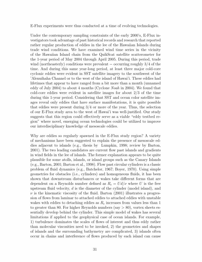
32

nents of the Ekman transport, τx and τy (both in N m−2) are the eastward andnorthward components of wind stress, ρ is the density of seawater (kg m−3),and f (sec−1) is the local Coriolis parameter given by f = 2Ωsinθ where Ω isthe Earth’s rotation rate and θ is the latitude of the observations. The shearlines in wind speed thus result in strong gradients in Ekman transports (pro-portional to the wind speed squared) that are directed to the right of the windvectors illustrated in Figures 2a, b, and c and 11a, b, and c. The net effect isthen to produce alternating patterns of upper ocean layer convergences anddivergences downstream of the islands. In the converging zones, downwellingof near surface water occurs whereas in diverging zones, upwelling of subsub-surface waters occurs. This condition sets the stage for the spin-up of cold-coremesoscale eddies and warm-core anti-cyclonic eddies as either relatively coolor relatively warm waters are isolated via flow instabilities and rotational ef-fects. The spatial wind vector field distribution derived from QuikScat hasbeen used to compute upwelling and downwelling velocity, w, via the Ekmanpumping mechanism (e.g., Chavanne et al., 2002) according to
w =1
ρf
[∆τy∆x
− ∆τx∆y
](2)
where w is in m s−1, and ∆τy/∆x and ∆τx/∆y are orthogonal gradients inwind stress. The final term in brackets in equation 2, [∆τy/∆x - ∆τx/∆y],is called the wind stress curl, so local vertical velocity is proportional to thewind stress curl as both ρ and f are effectively constant for our case. Usingthe wind fields displayed in Figures 2c, 7a, and 11c for E-Flux I, II, and III,respectively, we have computed the wind stress curl and Ekman pumping ve-locities, the latter shown in Figures 16a − f. The wind stress curl field tends totake the form of dipole-like structures displaying positive values on the north-ern sides and negative values on the southern sides of the wind stress maxima.These lee effects often extend several island diameter scales downwind as evi-denced in SST images shown in Figures 2b, and c and 11b, and c. Figures 16aand e clearly show that during trade wind conditions (before E-Flux I andIII), strong upwelling patterns occur with values reaching maximum values ofroughly 1.5-2.5 m day−1 just downwind of the ’Alenuihaha Channel where wealso see the formation of cyclonic eddies (i.e., Cyclone Noah during E-Flux Iand Cyclone Opal during E-Flux III). These values are comparable to thosereported in the same general oceanic region by Chavanne et al. (2002), whoreported values of about 3 m day−1. They commented that instantaneous val-ues may well be higher and our coarse resolution of the wind field would alsosuggest that values presented here are likely lower limit estimates. Because ofthe Ekman pumping, the local thermoclines must necessarily be lifted in up-welling areas and depressed in downwelling zones. This effect likely contributesto the formation of cold-core cyclones and warm-core anti-cyclones that areso often evident downstream of the Hawaiian Islands during persistent trade
33

wind conditions. Note that the wind stress curl field and thus distribution ofvertical velocities before and during E-Flux II (Figures 16c and d) is ratherfeatureless. This lack of wind shear, small wind stress curl, and weak localizedupwelling and downwelling velocities supports the argument that eddies arelikely produced via the wind forcing mechanism rather than others such asoceanic flow. Calil et al. (this volume) have recently done detailed numericalmodeling simulations of the ocean response to realistic wind forcing in thelee of the Hawaiian Island chain, which are valuable for improving our under-standing of the physical processes reported in our study. Also, Chavanne et al.(2002) did studies of wind forcing and oceanic responses for the Cabo Verdearchipelago off the west coast of Africa.
Considerable research concerning island effects on ocean flows and biologicalprocesses has been conducted in the region of the Canary Islands (e.g., Barton,2001; Aristegui et al., 1994, 1997; Barton et al., 2000, 2001, 2004; Basterretxeaet al., 2002). The Canaries are high volcanic islands that are located wherestrong southwestward trade winds blow. The geophysical setting has severalsimilarities to the Hawaiian Islands. Both the current flow and wind stressgradient mechanisms have been invoked to explain eddies in the wakes of theCanary Islands (e.g., Barton, 2001). One complication presented for CanaryIsland studies is the coastal effect of filaments that can interact with eddies(e.g., Barton et al., 2004). Nonetheless, comparative studies of physical andbiological phenomena occurring in the Hawaiian, Canary, and Cabo VerdeIslands should prove to be quite valuable, especially when model simulationscan be done in conjunction with comprehensive field experiments.
5 Summary
The two major eddies that occurred to the west of Hawai’i during the pe-riod of May 2004 to April 2005 coincided with periods of strong trade winds.Cyclone Noah likely formed to the southwest of the ’Alenuihaha Channel inmid-August, over 2 1/2 months before the first E-Flux field experiment. Cy-clone Noah appears to have formed shortly after another cold-core cyclone(unnamed) had drifted westward away from the ’Alenuihaha Channel area.Both of these features occurred during prolonged and strong trade wind con-ditions. The former unnamed eddy appears to have a lifetime of about 4-6weeks whereas Noah, which existed for at least 4 months, was the longest-lived cyclone observed off Hawai’i during the study year. The E-Flux I fieldsampling began about 3 months after Noah’s spin-up, indicating that the ma-ture to perhaps decaying phase was observed. The strong currents (∼80 cmsec−1) and well-developed doming of isotherms, isopycnals, nutrient isopleths,and chlorophyll a isopleths along with outcropping of some of the isoplethsin the environs of the center of the eddy all suggest that Noah was still a
34
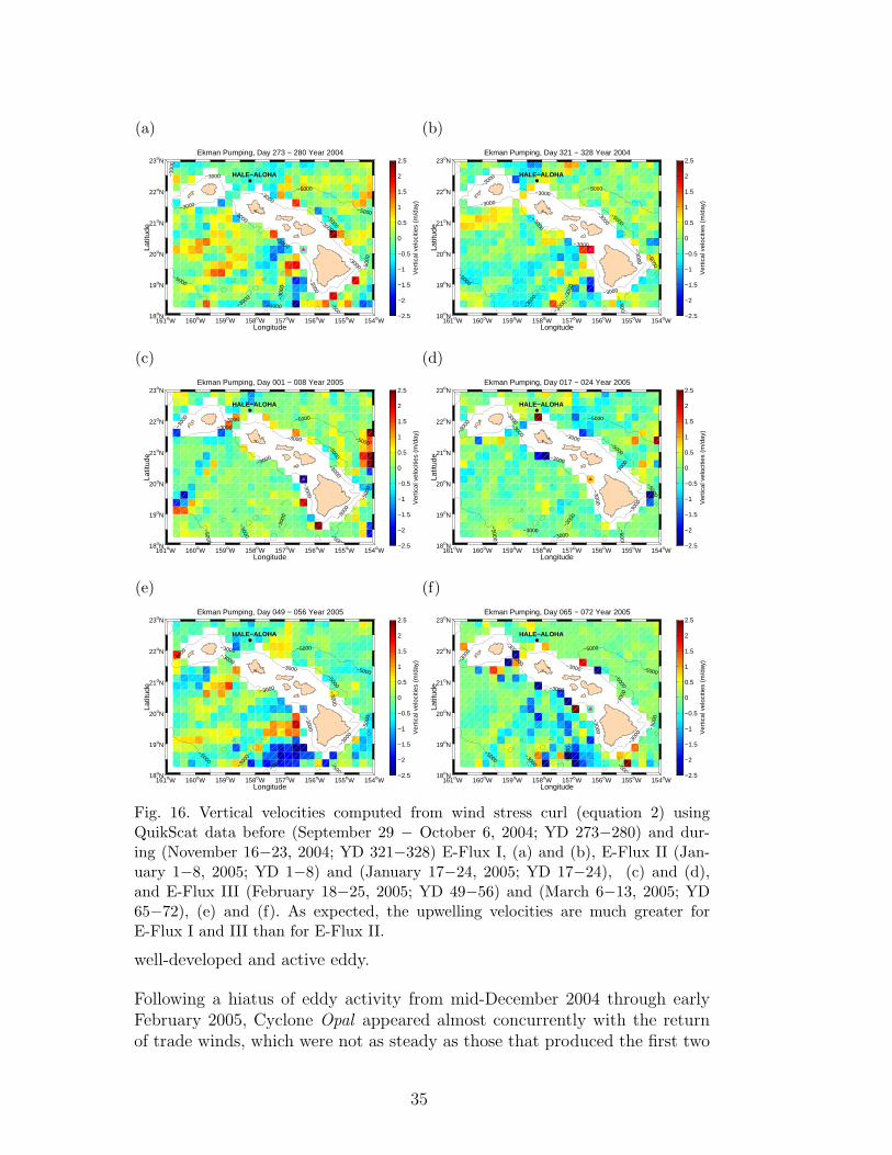
(a)
−5000
−5000
−500
0
−5000
−5000
−5000
−30
00
−3000−3000
−3000
−3000
−3000
−3000
−3000
−3000
−3000 −30
00
−3000
161oW 160oW 159oW 158oW 157oW 156oW 155oW 154oW 18oN
19oN
20oN
21oN
22oN
23oN
HALE−ALOHA
Longitude
Latit
ude
Ekman Pumping, Day 273 − 280 Year 2004
Ver
tical
vel
ociti
es (
m/d
ay)
−2.5
−2
−1.5
−1
−0.5
0
0.5
1
1.5
2
2.5
(b)
−5000
−5000
−5000
−5000
−5000
−3000
−3000
−3000
−3000
−3000
−3000
−3000
−3000
−300
0 −300
0
−300
0
161oW 160oW 159oW 158oW 157oW 156oW 155oW 154oW 18oN
19oN
20oN
21oN
22oN
23oN
HALE−ALOHA
Longitude
Latit
ude
Ekman Pumping, Day 321 − 328 Year 2004
Ver
tical
vel
ociti
es (
m/d
ay)
−2.5
−2
−1.5
−1
−0.5
0
0.5
1
1.5
2
2.5
(c)
−5000
−5000
−500
0
−5000
−5000
−5000
−3000
−3000
−3000
−300
0
−3000
−3000
−3000
−300
0
−3000
−300
0
161oW 160oW 159oW 158oW 157oW 156oW 155oW 154oW 18oN
19oN
20oN
21oN
22oN
23oN
HALE−ALOHA
Longitude
Latit
ude
Ekman Pumping, Day 001 − 008 Year 2005
Ver
tical
vel
ociti
es (
m/d
ay)
−2.5
−2
−1.5
−1
−0.5
0
0.5
1
1.5
2
2.5
(d)
−5000
−5000
−5000
−5000
−5000
−3000
−3000
−3000
−300
0
−300
0
−3000
−3000
−300
0
−3000
−300
0
−3000
161oW 160oW 159oW 158oW 157oW 156oW 155oW 154oW 18oN
19oN
20oN
21oN
22oN
23oN
HALE−ALOHA
Longitude
Latit
ude
Ekman Pumping, Day 017 − 024 Year 2005
Ver
tical
vel
ociti
es (
m/d
ay)
−2.5
−2
−1.5
−1
−0.5
0
0.5
1
1.5
2
2.5
(e)
−5000−5000
−500
0
−5000
−5000
−5000
−3000
−3000
−3000
−300
0
−3000
−3000
−3000
−3000
−300
0 −30
00
−3000
161oW 160oW 159oW 158oW 157oW 156oW 155oW 154oW 18oN
19oN
20oN
21oN
22oN
23oN
HALE−ALOHA
Longitude
Latit
ude
Ekman Pumping, Day 049 − 056 Year 2005
Ver
tical
vel
ociti
es (
m/d
ay)
−2.5
−2
−1.5
−1
−0.5
0
0.5
1
1.5
2
2.5
(f)
−5000−5000
−500
0
−5000
−5000
−5000
−3000
−3000
−3000
−300
0
−300
0
−3000
−3000
−300
0
−3000
−30
00
161oW 160oW 159oW 158oW 157oW 156oW 155oW 154oW 18oN
19oN
20oN
21oN
22oN
23oN
HALE−ALOHA
Longitude
Latit
ude
Ekman Pumping, Day 065 − 072 Year 2005
Ver
tical
vel
ociti
es (
m/d
ay)
−2.5
−2
−1.5
−1
−0.5
0
0.5
1
1.5
2
2.5
Fig. 16. Vertical velocities computed from wind stress curl (equation 2) usingQuikScat data before (September 29 − October 6, 2004; YD 273−280) and dur-ing (November 16−23, 2004; YD 321−328) E-Flux I, (a) and (b), E-Flux II (Jan-uary 1−8, 2005; YD 1−8) and (January 17−24, 2005; YD 17−24), (c) and (d),and E-Flux III (February 18−25, 2005; YD 49−56) and (March 6−13, 2005; YD65−72), (e) and (f). As expected, the upwelling velocities are much greater forE-Flux I and III than for E-Flux II.
well-developed and active eddy.
Following a hiatus of eddy activity from mid-December 2004 through earlyFebruary 2005, Cyclone Opal appeared almost concurrently with the returnof trade winds, which were not as steady as those that produced the first two
35
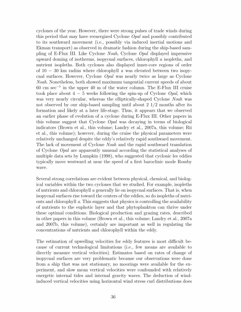
cyclones of the year. However, there were strong pulses of trade winds duringthis period that may have reenergized Cyclone Opal and possibly contributedto its southward movement (i.e., possibly via induced inertial motions andEkman transport) as observed in dramatic fashion during the ship-based sam-pling of E-Flux III. Like Cyclone Noah, Cyclone Opal displayed impressiveupward doming of isotherms, isopycnal surfaces, chlorophyll a isopleths, andnutrient isopleths. Both cyclones also displayed inner-core regions of orderof 10 − 30 km radius where chlorophyll a was elevated between two isopy-cnal surfaces. However, Cyclone Opal was nearly twice as large as CycloneNoah. Nonetheless, both showed maximum tangential current speeds of about60 cm sec−1 in the upper 40 m of the water column. The E-Flux III cruisetook place about 4 − 5 weeks following the spin-up of Cyclone Opal, whichwas very nearly circular, whereas the elliptically-shaped Cyclone Noah wasnot observed by our ship-based sampling until about 2 1/2 months after itsformation and likely at a later life-stage. Thus, it appears that we observedan earlier phase of evolution of a cyclone during E-Flux III. Other papers inthis volume suggest that Cyclone Opal was decaying in terms of biologicalindicators (Brown et al., this volume; Landry et al., 2007a, this volume; Riiet al., this volume); however, during the cruise the physical parameters wererelatively unchanged despite the eddy’s relatively rapid southward movement.The lack of movement of Cyclone Noah and the rapid southward translationof Cyclone Opal are apparently unusual according the statistical analyses ofmultiple data sets by Lumpkin (1998), who suggested that cyclonic lee eddiestypically move westward at near the speed of a first baroclinic mode Rossbywave.
Several strong correlations are evident between physical, chemical, and biolog-ical variables within the two cyclones that we studied. For example, isoplethsof nutrients and chlorophyll a generally lie on isopycnal surfaces. That is, whenisopycnal surfaces rise toward the centers of the eddies, so do isopleths of nutri-ents and chlorophyll a. This suggests that physics is controlling the availabilityof nutrients to the euphotic layer and that phytoplankton can thrive underthese optimal conditions. Biological production and grazing rates, describedin other papers in this volume (Brown et al., this volume; Landry et al., 2007aand 2007b, this volume), certainly are important as well in regulating theconcentrations of nutrients and chlorophyll within the eddy.
The estimation of upwelling velocities for eddy features is most difficult be-cause of current technological limitations (i.e., few means are available todirectly measure vertical velocities). Estimates based on rates of change ofisopycnal surfaces are very problematic because our observations were donefrom a ship that was not stationary, no moorings were available for the ex-periment, and slow mean vertical velocities were confounded with relativelyenergetic internal tides and internal gravity waves. The deduction of wind-induced vertical velocities using horizontal wind stress curl distributions does
36

provide at least some order of magnitude estimates. However, spatial reso-lution of available satellite scatterometer data is insufficient to gain desiredaccuracy and spatial resolution. Clearly, models are sensitive to both goodestimates of vertical and horizontal velocities for computing advection termsand estimates of turbulent diffusion. Unfortunately, no measurements of mix-ing, diffusion, or turbulence parameters were possible under the budgetaryconstraints of the E-Flux program. Nonetheless, Nencioli et al., (this volume)have introduced some important ideas concerning nutrient inputs within Cy-clone Opal, hypothesizing a conceptual model in which the eddy acts more likean open bottom/horizontally leaky feature, rather than like a closed systemwith no exchanges with the surrounding waters.
Despite many similar gross features and scales, each ocean eddy is unique.For example, there are several different genesis mechanisms for eddies thatcontribute to different physical, chemical, and biological distributions withintheir interiors. For example, Gulf Stream and Kuroshio eddies tend to retainmaterials derived from adjacent waters. On the other hand, materials foundwithin Hawaiian lee eddies are likely locally produced suggesting that theseeddies are likely more representative of gyre eddies. However, the subsurfaceexpressions of the eddies studied during this experiment were relatively shal-low, perhaps because they were rather newly formed. The Hawaiian lee eddiesappear to go through several evolutionary stages and each translates along aunique path, presumably due to competing influences of the β-effects and flowconditions outside the eddy (i.e., in the atmosphere, hurricanes are steered byexternal wind patterns). There may well be eddy-eddy (vortex-vortex) inter-actions since cyclonic and anticyclonic eddies are often in close proximity inthe lee of the Hawaiian Islands (e.g., Lumpkin, 1998). Such interactions wouldalso likely affect the translations of the individual eddies. This aspect is con-sidered in more detail for Cyclone Opal in the paper by Nencioli et al. (thisvolume). It is clear that every eddy observation remains important for gainingnew insights into processes, increasing our understanding, and developing andtesting interdisciplinary models. Because we still have so few direct observa-tions of eddies and the data we are presently able to collect are so limited inthe number of key parameters and the spatial and temporal sampling, broadinferences and conclusions based on any single experiment or even a few suchexperiments must be considered in context. Future eddy research programsshould be able to capitalize on emerging platform and sensor technologies aswell as models using data assimilation and field programs using such modelsfor adaptive sampling (Dickey and Bidigare, 2005). The region selected for thepresent study is ideal for such eddy studies.
37

6 Acknowledgments
We would like to thank all of our E-Flux collaborators, particularly ClaudiaBenitez-Nelson, for their assistance in collecting the data described in this pa-per and for their intellectual contributions. Eric Firing and Jules Hammondprovided expert assistance with the ADCP data sets. The crews and techni-cians of the R/V KOK and R/V Wecoma are thanked for their assistance atsea. The valuable comments and suggestions of anonymous reviewers are mostmost appreciated as they significantly helped to strengthen the paper. Thisstudy was funded by the NSF Ocean Chemistry Program.
References
Allen, C. B., Kanda, J., Laws, E. A., 1996. New production and photosyntheticrates within and outside a cyclonic mesoscale eddy in the North Pacificsubtropical gyre. Deep-Sea Research I 43, 917 – 936.
Alsdorf, D., Fu, L. L., Mognard, N., Cazenave, A., Rodriguez, E., Chelton, D.,Lettenmaier, D., 2007. Measuring global oceans and terrestrial freshwaterfrom space. EOS, Transaction of the American Geophysical Union 88(24),253 – 257.
Aristegui, J., Sangra, P., Henandez-Leon, S., Canton, M., Hernandez-Guerra,A., 1994. Island-induced eddies in the Canary Islands. Deep-Sea Research I41, 1509 – 1525.
Aristegui, J., Tett, P., Hernandez-Guerra, A., Basterretxea, G., Montero,M. F., Wild, K., Sangra, P., Hernandez-Leon, S., Canton, M., Garcia-Braun,J. A., Pacheco, M., Barton, E. D., 1997. The influence of island-generatededdies on chlorophyll distribution: A study of mesoscale variation aroundGran Canaria. Deep-Sea Research I 44, 71 – 96.
Barton, E. D., 2001. Island wakes. In: Steele, J. H., Thorpe, S. A., Turekian,K. K. (Eds.), Encyclopedia of Ocean Sciences. Vol. 5. Academic Press, Or-lando, pp. 1397 – 1402.
Barton, E. D., Aristegui, J., Tett, P., Canton, M., Garcia-Braun, J.,Hernandez-Leon, S., Nykjaer, L., Almeida, J., Almunia, J., Ballesteros,S., Basterretxea, G., Escanez, J., Garcia-Weill, L., Hernandez-Guerra, A.,Lopez-Laatzen, F., Molina, R., Montero, M. F., Navarro-Perez, E., Ro-driguez, J. M., van Lenning, K., Velez, H., Wild, K., 1998. The transitionzone of the Canary Current upwelling region. Progress in Oceanography 41,455 – 504.
Barton, E. D., Aristegui, J., Tett, P., Perez, E. N., 2004. Variability in theCanary Islands area of filament-eddy exchanges. Progress in Oceanography62 (2-4), 71 – 94.
Barton, E. D., Basterretxea, G., Flament, P., Mitchelson-Jacob, E. G., Jones,
38

B., Aristegui, J., Herrera, F., 2000. Lee region of Gran Canaria. Journal ofGeophysical Research 105 (C7), 17173 – 17193.
Basterretxea, G., Barton, E. D., Tett, P., Sangra, P., Navarro-Perez, E., Aris-tegui, J., 2002. Eddy and deep chlorophyl maximum response to wind-shearin the lee of Gran Canaria. Deep-Sea Research I 49 (6), 1087 – 1101.
Batchelor, G. K., 1967. An Introduction to Fluid Dynamics. Cambridge Uni-versity Press.
Benitez-Nelson, C., Bidigare, R. R., Dickey, T. D., Landry, M. R., Leonard,C. L., Brown, S. L., Nencioli, F., Rii, Y. M., Maiti, K., Becker, J. W., Bibby,T. S., Black, W., Cai, W. J., Carlson, C. A., Chen, F., Kuwahara, V. S.,Mahaffey, C., McAndrew, P. M., Quay, P. D., Rappe, M. S., Selph, K. E.,Simmons, M. P., Yang, E. J., 2007. Mesoscale eddies drive increased silicaexport in the subtropical Pacific Ocean. Science 316, 1017 – 1020.
Bidigare, R. R., Benitez-Nelson, C., Leonard, C. L., Quay, P. D., Parsons,M. L., Foley, D. G., Seki, M. P., 2003. Influence of a cyclonic eddy on mi-croheterotroph biomass and carbon export in the lee of Hawaii. GeophysicalResearch Letters 30(6), 1318.
Boyer, D. L., 1970. Flow past a right circular cylinder in a rotating frame.Journal of Basic Engineering 92 (3), 430 – 436.
Brown, S. L., Landry, M. R., Selph, K. E., 2007. Diatoms in the desert. Deep-Sea Research II, this volume.
Calil, P. H. R., Richards, K. J., Jia, Y., Bidigare, R. R., 2007. Eddy activityin the lee of the Hawaiian Islands. Deep-Sea Research II, this volume.
Campbell, J. W., Blaisdell, J. M., Darzi, M., 1995. Level-3 SeaWiFS data prod-ucts: Spatial and temporal binning algorithms, NASA Tech. Memo. Tech.Rep. 104566, NASA Goddard Space Flight Center, Greenbelt, Maryland.
Chassignet, E. P., Cushman-Roisin, B., 1991. On the influence of a lowerlayer on the propagation of nonlinear oceanic eddies. Journal of PhysicalOceanography 21 (7), 939 – 957.
Chavanne, C., Flament, P., Lumpkin, R., Dousset, B., Bentamy, A., 2002.Scatterometer observations of wind variations induced by oceanic islands:Implications for wind-driven ocean circulation. Canadian Journal of RemoteSensing 28(3), 466 – 474.
Chen, Y. L., Feng, J., 1995. The influences of inversion height on precipitationand air-flow over the island of Hawaii. Monthly Weather Review 123 (6),1660 – 1676.
Cheney, R. E., Richardson, P. L., 1976. Observed decay of a cyclonic GulfStream ring. Deep-Sea Research 23 (2), 143 – 155.
Cushman-Roisin, B., Chassignet, E. P., Tang, B., 1990. Westward motion ofmesoscale eddies. Journal of Physical Oceanography 20 (5), 758 – 768.
Dickey, T. D., Bidigare, R. R., 2005. Interdisciplinary oceanographic observa-tions: the wave of the future. Scientia Marina 69(Suppl. 1), 23 – 42.
Dickey, T. D., Granata, T., Marra, J., Langdon, C., Wiggert, J., Chai-Jochner,Z., Hamilton, M., Vasquez, J., Stramska, M., Bidigare, R. R., 1993. Seasonalvariability of bio-optical and physical properties in the Sargasso Sea. Journal
39

of Geophysical Research 98, 865 – 898.Falkowski, P. G., Ziemann, D., Kolber, Z., Bienfang, P. K., 1991. Role of eddy
pumping in enhancing primary production in the ocean. Nature 352, 55 –58.
Fischer, A. S., Weller, R. A., Rudnick, D. L., Eriksen, C. C., Lee, C. M., Brink,K. H., Fox, C. A., Leben, R. R., 2002. Mesoscale eddies, coastal upwelling,and the upper-ocean heat budget in the Arabian Sea. Deep-Sea Research II49 (12), 2231 – 2264.
Flierl, G. R., McGillicuddy, D. J., 2002. Mesoscale and submesoscale physical-biological interactions. In: Robinson, A. R., McCarthy, J. J., Rothschild, B.(Eds.), Biological-Physical Interactions in the Sea. Vol. 12 of The Sea. JohnWiley & Sons, New York, Ch. 4, pp. 113 – 185.
Garcon, V., Oschlies, A., Doney, S. C., McGillicuddy, D. J., Waniek, J., 2001.The role of mesoscale variability on plankton dynamics in the North At-lantic. Deep-Sea Research II 48, 2199 – 2226.
Holland, C. L., Mitchum, G. T., 2001. Propagation of Big Island eddies. Jour-nal of Geophysical Research 106 (C1), 935 – 944.
Honjo, S., Dymond, J., Prell, W., Ittekkot, V., 1999. Monsoon-controlled ex-port fluxes to the interior of the Arabian Sea. Deep-Sea Research II 46 (8-9),1859 – 1902.
Kuwahara, V. S., Nencioli, F., Dickey, T. D., Rii, Y. M., Bidigare, R. R., 2007.Physical dynamics and biological implications of cyclone Noah in the lee ofHawai’i during E-Flux I. Deep-Sea Research II, this volume.
Landry, M. R., Brown, K. E., Selph, K. E., Simmons, M. P., Rii, Y. M., 2007a.Depth-stratified phytoplankton dynamics in Cyclone Opal, a subtropicalmesoscale eddy. Deep-Sea Research II, this volume.
Landry, M. R., Decima, M., Simmons, M. P., Hannides, C. C. S., Daniels, E.,2007b. Mesozooplankton biomass and grazing responses to Cyclone Opal, asubtropical mesoscale eddy. Deep-Sea Research II, this volume.
Leonard, C. L., Bidigare, R. R., Seki, M. P., Polovina, J. J., 2001. Interannualmesoscale physical and biological variability in the North Pacific CentralGyre. Progress in Oceanography 49 (1-4), 227 – 244.
Letelier, R. M., Karl, D. M., Abbott, M. R., Flament, P., Freilich, M., Lukas,R., Strub, T., 2000. Role of late winter mesoscale events in the biogeochem-ical variability of the upper water column of the North Pacific SubtropicalGyre. Journal of Geophysical Research 105 (C12), 28723 – 28739.
Lewis, M. R., 2007. Variability of plankton and plankton processes on themesoscale. In: Williams, P. J. l. B., Thomas, D. N., Reynolds, C. S. (Eds.),Phytoplankton Productivity: Carbon Assimilation in Marine and Freshwa-ter Ecosystems. Blackwell Science, Oxford, UK, Ch. 6, pp. 141 – 155.
Lobel, P. S., Robinson, A. R., 1986. Transport and entrapment of fish larvae byocean mesoscale eddies and currents in Hawaiian waters. Deep-Sea Research33(4), 483 – 500.
Lumpkin, C. F., 1998. Eddies and currents in the Hawaii islands. Ph.D. thesis,University of Hawaii.
40

McGillicuddy, D. J., Robinson, A. R., 1997. Eddy-induced nutrient supplyand new production in the Sargasso Sea. Deep-Sea Research I 44(8), 1427– 1450.
McGillicuddy, D. J., Robinson, A. R., Siegel, D. A., Jannasch, H. W., John-son, R., Dickey, T. D., McNeil, J. D., Michaels, A. F., Knap, A. H., 1998.Influence of mesoscale eddies on new production in the Sargasso Sea. Nature394, 263 – 266.
McNeil, J. D., Jannasch, H. W., Dickey, T. D., McGillicuddy, D. J., Brzezin-ski, M., Sakamoto, C. M., 1999. New chemical, bio-optical and physicalobservations of upper ocean response to the passage of a mesoscale eddy offBermuda. Journal of Geophysical Research 104, 15537 – 15548.
Morel, A., 1988. Optical modeling of the upper ocean in relation to itsbiogenous matter content (Case I waters). Journal of Geophysical Research93(C9), 10749 – 10768.
Nencioli, F., Kuwahara, V. S., Dickey, T. D., Rii, Y. M., Bidigare, R. R.,2007. Physical dynamics and biological implications of a mesoscale eddy inthe lee of Hawai’i: Cyclone Opal observations during E-Flux III. Deep-SeaResearch II, this volume.
Olson, D. B., 1980. The physical oceanography of two rings observed by theCyclonic Ring Experiment, Part II: dynamics. Journal of Physical Oceanog-raphy 10, 514 – 527.
Oschlies, A., 2001. Model-derived estimates of new production: New resultspoint towards lower values. Deep-Sea Research II 48 (10), 2173 – 2197.
Oschlies, A., Garcon, V., 1998. Eddy-induced enhancement of primary pro-duction in a model of the North Atlantic Ocean. Nature 394, 266 – 269.
Patzert, W. C., 1969. Eddies in Hawaiian Islands. Tech. Rep. HIG-69-8, HawaiiInstitute of Geophysics, University of Hawaii.
Qiu, B., Koh, D. A., Lumpkin, C., Flament, P., 1997. Existence and forma-tion mechanism of the North Hawaiian Ridge Current. Journal of PhysicalOceanography 27, 431 – 444.
Richman, J. G., Wunsch, C., Hogg, N. G., 1977. Space and time scales ofmesoscale motion in the western North Atlantic. Reviews of Geophysics15 (4), 385 – 420.
Rii, Y. M., Brown, S. L., Nencioli, F., Kuwahara, V. S., Dickey, T. D., Karl,D. M., Bidigare, R. R., 2007. The transient oasis: nutrient-phytoplanktondynamics and particle export in Hawaiian lee cyclones. Deep-Sea ResearchII, this volume.
Sakamoto, C. M., Karl, D. M., Jannasch, H. W., Bidigare, R. R., Letelier,R. M., Walz, P. M., Ryan, J. P., Polito, P. S., Johnson, K. S., 2004. Influ-ence of Rossby waves on nutrient dynamics and the plankton communitystructure in the North Pacific subtropical gyre. Journal of Geophysical Re-search 109 (C5).
Seki, M. P., Lumpkin, R., Flament, P., 2002. Hawaii cyclonic eddies and bluemarlin catches: the case study of the 1995 Hawaiian International BillfishTournament. Journal of Oceanography 58, 739 – 745.
41

Seki, M. P., Polovina, J. J., Brainard, R. E., Bidigare, R. R., Leonard, C. L.,Foley, D. G., 2001. Biological enhancement at cyclonic eddies tracked withGOES thermal imagery in Hawaiian waters. Geophysical Research Letters28(8), 1583 – 1586.
Smith, R. B., Grubisic, V., 1993. Aerial observations of Hawaii’s wake. Journalof Atmospheric Sciences 50 (22), 3728 – 3750.
Smith, S. D., 1988. Coefficients for sea-surface wind stress, heat-flux, and windprofiles as a function of wind-speed and temperature. Journal of GeophysicalResearch 93 (C12), 15467 – 15472.
Stumpf, H. G., Legeckis, R. V., 1977. Satellite-observations of mesoscale eddydynamics in the eastern tropical Pacific Ocean. Journal of Physical Oceanog-raphy 7 (5), 648 – 658.
Taupier-Letage, I., Puillat, I., Millot, C., Raimbault, P., 2003. Biological re-sponse to mesoscale eddies in the Algerian Basin. Journal of GeophysicalResearch 108 (C8), 3245.
UNESCO, 1981. Tenth report of the Joint Panel on Oceanographic Tables andStandards. Tech. rep., UNESCO Technical Papers in Marine Science.
Vaillancourt, R. D., J, M., Seki, M. P., Parsons, M. L., Bidigare, R. R., 2003.Impact of a cyclonic eddy on phytoplnkton community structure and pho-tosynthetic competency in the subtropical North Pacific Ocean. Deep-SeaResearch I 50, 829 – 847.
Xie, S. P., Liu, W. T., Liu, Q. Y., Nonaka, M., 2001. Far-reaching effectsof the Hawaiian islands on the Pacific Ocean-atmosphere system. Science292 (5524), 2057 – 2060.
42
Related Documents