Numerical Investigation of 3D Scanned Mooring Chains Effects of Stress Concentrations from Corrosion Pits Truls Johan Martin Braut Bache Master of Science in Mechanical Engineering Supervisor: Per Jahn Haagensen, KT Co-supervisor: Jochen Köhler, KT Department of Structural Engineering Submission date: February 2017 Norwegian University of Science and Technology

Welcome message from author
This document is posted to help you gain knowledge. Please leave a comment to let me know what you think about it! Share it to your friends and learn new things together.
Transcript

Numerical Investigation of 3D ScannedMooring ChainsEffects of Stress Concentrations from
Corrosion Pits
Truls Johan Martin BrautBache
Master of Science in Mechanical Engineering
Supervisor: Per Jahn Haagensen, KTCo-supervisor: Jochen Köhler, KT
Department of Structural Engineering
Submission date: February 2017
Norwegian University of Science and Technology


I
MASTER THESIS 2017
SUBJECT AREA:
3D scanning, fatigue, steel structures
DATE:
7 February 2017
NO. OF PAGES:
14 + 81 + 6
TITLE:
Numerical Investigation of 3D Scanned Mooring Chains Effects of Stress Concentrations from Corrosion Pits
BY:
Truls Braut Bache
RESPONSIBLE TEACHER: Professor Per Jahn Haagensen SUPERVISORS: Professor Per Jahn Haagensen, Professor Jochen Köhler CARRIED OUT AT: The Department of Structural Engineering, NTNU
SUMMARY: This thesis aims to numerically evaluate severe corrosion pits on offshore mooring chain. Pitting corrosion is considered a significant degradation mechanism as cracks tend to nucleate and propagate in areas of high stress concentration. Hence, the idea has been to replicate the pits using a 3D scanner, and subsequently analyze the pits in a finite element software. The study is part of a collaborative research project between Statoil ASA and NTNU, where the motivation is the fatigue life of offshore mooring lines. It is believed that surface conditions, like pitting corrosion, are highly influential on the chain segments fatigue life. The final aim is to introduce clear criteria for deciding whether a chain is too damaged to continue service or not. A method for replicating and evaluating the effects of the corrosion pits has been devised in the following. However, before it can be used on an actual situation, the methods capabilities need to be proved for a simple scenario. Consequently, this thesis has focused on developing the method and testing it on artificially made corrosion pits.

Master’s Thesis 2017
II

Master’s Thesis 2017
III
Preface This thesis is written on the behalf of the Department of Structural Engineering at the Norwegian University of Science and Technology (NTNU). It concludes my master’s degree in Mechanical Engineering and includes 22 weeks of work during the fall of 2016, as well as January 2017. The study emerged through a collaboration between NTNU and Statoil ASA, and is part of a larger project to investigate the fatigue life of offshore mooring chains based on their surface conditions. The paper is focused on numerical analyses of 3D-scanned surfaces – a method for preparing the surface and relevant surface parameters are of the essence. To understand the problem and the scope of it, an introduction concerning the mooring lines have been added in the beginning. The target group for this study is engineers working with offshore structures, or individuals which have an interest for fatigue analysis. I want to thank my supervisors Jochen Köhler and Per Jahn Haagensen at the Department of Structural Engineering at NTNU. Your help and guidance have been essential for the results of this thesis. I would further like to extend my gratitude to some of the technical staff at the department – this work could never have been finished without the help of Christian Frugone, Gøran Loraas and Odd Kristian Nerdahl. Finally, I would like to thank my former student colleagues, Alexander Hoel, Martin Hove and Kristin Tømmervåg, whom I first had the pleasure of working alongside, before I inherited their final work. Trondheim 06.02.2017. Truls Braut Bache

Master’s Thesis 2017
IV

Master’s Thesis 2017
V
Abstract Pitting corrosion is an extreme form of localized corrosion characterized by the formation of pits that penetrate into the metal, resulting in mass loss. This thesis aims to evaluate the severe corrosion pits often seen to develop on offshore mooring lines after some years of use. As fatigue cracks tend to nucleate and propagate from areas of high stress concentration, these pits are considered a significant degradation mechanism. Using an industrial 3D-scanner, the idea is to replicate the corrosion pits for subsequent analysis in a FEM software. However, before it can be used on an actual situation, the methods capabilities need to be proved for a simple scenario. Consequently, this work has been based on identifying critical parameters on the chain surface, and establishing a reliable procedure for numerically analyzing the scans. Finally, the method has been tested for a simple case of steel tensile specimens with machined artificial pits. An ATOS III SO 3D-scanner has been used for the replicating of surfaces. The scans have subsequently been processed and meshed in GeoMagic Studio 14 and ANSYS ICEM CFD 17.0, before they have been analyzed in ABAQUS/CAE 6.14. A linear elastic material model has been used, as the only aim was to establish a maximum stress concentration factor (SCF). Before meshing, the surfaces have been converted into CAD-surfaces, using a mathematical model called NURBS. This procedure is done automatically in GeoMagic Studio 14. The machined pits are based on realistic approximations of actual corrosion pits. They display a depth of 4 mm and a diameter of 8 mm. Furthermore, they are divided into two categories; hemispherical pits and conical pits. The conical ones generally demonstrate the highest SCF, in the range of 𝐾𝑡
′ = 2.6. The final simulations are promising, displaying analogous results to relevant analytical solutions of notch geometries. Simulation predictions seem to correspond well with the actual failure locations, whereas the fatigue life predictions are more uncertain, producing too conservative results. Presence of compressive residual stress is suggested as a possible cause for the error in life estimation.

Master’s Thesis 2017
VI

Master’s Thesis 2017
VII
Sammendrag Korrosjonsgroper er en ekstrem form for lokal korrosjon som kan kjennetegnes ved groper som penetreres inn i metall, og dermed resulterer i materialtap. Denne avhandlingen sikter mot å evaluere alvorlige korrosjonsgroper som ofte er å finne på gamle offshore-konstruksjoner etter flere år i bruk. Ettersom utmattingssprekker gjerne etableres og utvikles fra områder med høye spenningskonsentrasjoner, er disse gropene ansett som en betydelig degraderingsmekanisme. Ved bruk av en industriell 3D-scanner har tanken vært å gjenskape disse korrosjonsgropene, for så å etterhvert analysere dem gjennom en elementanalyse (FEM). Men før dette kan bli brukt på de faktiske tilfellene, må metodens evner bli testet for et enkelt scenario. Derfor har det følgende arbeidet blitt basert på å identifisere kritiske parametere for kjettingoverflatene, og etterhvert etablere troverdige prosedyrer for å numerisk analysere de respektive gjenskapningene. Til slutt har metoden blitt testet for et enkelt tilfelle med kunstige korrosjonsgroper maskinert inn i strekkprøver. En ATOS III SO 3D-skanner har blitt brukt for å gjenskape overflatene. De skannede overflatene har etterhvert blitt bearbeidet og tilordnet et mesh gjennom programmene GeoMagic Studio 14 og ANSYS ICEM CFD 17.0, før de har blitt analysert i ABAQUS/CAE 6.14. En lineær elastisk materialmodell har blitt brukt ettersom vi bare er ute etter en maksimal spenningskonsentrasjonsfaktor. Forut tilordningen av mesh finner sted, har overflaten blitt gjort om til en CAD-overflate, ved hjelp av en matematisk modell kalt NURBS. Denne omgjøringen blir gjort automatisk i GeoMagic Studio 14. De maskinerte gropene er basert på realistiske tilnærminger av faktiske korrosjonsgroper. De fremviser en dybde på 4 mm og en diameter på 8 mm. Videre er de delt opp i to kategorier; halvkuleformet grop og konisk grop. De koniske gropene har generelt sett en høyere spenningskonsentrasjonsfaktor, som ligger i et område rundt 𝐾𝑡
′ = 2.6. De endelige simuleringene viser lovende resultater, som kan relateres til relevante analytiske løsninger for idealiserte gropgeometrier. Prediksjoner etablert fra simuleringene passer godt med de faktiske bruddområdene. Dette er imidlertid ikke helt tilfellet for de predikterte levetidsberegningene, som ser ut til å være for konservative sammenlignet med de faktiske resultatene. Tilstedeværelsen av kompresjonsrestspenninger er forslått som en mulig forklaring på dette.

Master’s Thesis 2017
VIII

Master’s Thesis 2017
IX
Nomenclature 𝑎 Depth of pit/notch 𝑏 Fatigue strength exponent 𝐶 Fitting constant – intercept of N-axis 𝐶𝑓 Correction factor of regression line to reference S-N curve
𝐶𝑓2 Correction factor of FEA regression line to test regression line
𝐶𝑠 Correction factor for surface conditions 𝑑 Diameter 𝐻 Width ℎ Thickness ℎ𝐾 Diameter of inscribed circle 𝐾𝑒 Effective stress concentration factor 𝐾𝑓 Fatigue stress concentration factor
𝐾𝑡 Theoretical stress concentration factor (stress/bending) 𝐾𝑡𝑠 Theoretical stress concentration factor (torsion) 𝐾𝑡𝑔 Theoretical stress concentration factor for gross cross-sectional 𝜎𝑛𝑜𝑚
𝐾𝑡𝑛 Theoretical stress concentration factor for net cross-sectional 𝜎𝑛𝑜𝑚 𝐾𝑡𝑥 Theoretical stress concentration factor in axial direction 𝐾𝑡𝜃 Theoretical stress concentration factor in circumferential direction 𝐾𝑡′ Theoretical stress concentration from maximum von Mises stress
𝐿 Length 𝑚 Fitting constant – negative slope 𝑁 Number of stress cycles 𝑁𝑖 Crack initiation period 𝑁𝑝 Crack propagation period
𝑃 Applied load 𝑞 Notch sensitivity 𝑅 Load ratio 𝑅𝑡 Maximum peak-to- valley height 𝑅𝑧 Ten-point height 𝑅𝑎 Center line average roughness 𝑅𝑞 Root mean square roughness
𝑟 Radius of notch/pit 𝑟𝜅 Radius of curvature 𝑠log(𝑁) Standard deviation of log(N)
𝑉 Volume of element 𝜈 Poisson’s ratio 𝜅 Curvature 𝜎 Applied stress 𝜎𝑎 Stress amplitude 𝜎𝑎𝑟 Zero equivalent mean stress 𝜎𝑒𝑞 Equivalent stress/von Mises stress
𝜎𝑓 Fatigue limit of unnotched specimen
𝜎𝑛𝑓 Fatigue limit of notched specimen
𝜎𝑓′ Fatigue strength coefficient
𝜎𝑙𝑜𝑐𝑎𝑙 Local stress in component 𝜎𝑚 Mean stress 𝜎𝑚𝑎𝑥 Maximum stress 𝜎𝑚𝑖𝑛 Minimum stress

Master’s Thesis 2017
X
𝜎𝑛 Stress in net cross-sectional area 𝜎𝑛𝑜𝑚 Nominal stress in component 𝜎𝑥 Stress in axial direction 𝜎𝑦 Yield strength
𝜎1, 𝜎2, 𝜎3 Principal stresses 𝜎𝜃 Stress in circumferential direction ∆𝜎 Stress range ∆𝜎𝑚𝑜𝑑 Modified fatigue limit ∆𝜎0 Fatigue limit 𝜏𝑚𝑎𝑥 Maximum shear stress 𝜏𝑛𝑜𝑚 Nominal shear stress

Master’s Thesis 2017
XI
Acronyms bpd Barrels per day CAD Computer Aided Design DNV-GL Det Norske Veritas – Germanischer Lloyd EAC Environmental Assisted Cracking FEA Finite Element Analysis FEM Finite Element Method FPS Floating Production System FPSO Floating Production, Storage and Offloading FSO Floating, Storage and Offloading GBP British Pounds GOM Gesellschaft fur OptischeMesstechnik mbH GS14 GeoMagic Studio 14 IACS International Association of Classification Societies ICEM ANSYS ICEM CFD 17.0 ISO International Organization of Standardization JIP Joint Industry Project LPI Liquid Penetrant Testing MPI Magnetic Particle Inspection NCS Norwegian Continental Shelf NDT Non-Destructive Testing NTNU Norwegian University of Science and Technology NURBS Non-Uniform Rotational B-Spline PSA Petroleum Safety Authority Norway RNNP Trends in risk level in the petroleum activity SCF Stress Concentration Factor SPM Single Point Mooring SM Spread Mooring S-N curve Stress-Life curve

Master’s Thesis 2017
XII

Master’s Thesis 2017
XIII
Contents
Preface ............................................................................................................................ III
Abstract ............................................................................................................................ V
Sammendrag .................................................................................................................. VII
Nomenclature .................................................................................................................. IX
Acronyms ........................................................................................................................ XI
Contents ........................................................................................................................ XIII
1 Introduction .............................................................................................................. 1 1.1 Previous Studies ........................................................................................................... 1 1.2 Objective of Study ........................................................................................................ 2 1.3 Scope of Study ............................................................................................................. 2 1.4 Overview of Thesis ....................................................................................................... 3
2 Offshore Mooring Lines ............................................................................................. 4 2.1 Mooring Systems.......................................................................................................... 4 2.2 Mooring Lines .............................................................................................................. 6 2.3 Mooring Failure ............................................................................................................ 9
2.3.1 A Financial Perspective ...................................................................................................... 9 2.3.2 Failure Statistics ................................................................................................................. 9
2.4 Inspection Today ........................................................................................................ 11
3 Fatigue .................................................................................................................... 12 3.1 The Basics of Fatigue .................................................................................................. 12 3.2 Fatigue Life Curves ..................................................................................................... 13 3.3 Assessment of Fatigue ................................................................................................ 14 3.4 Type of Loading .......................................................................................................... 15 3.5 Stress Concentration Factors ...................................................................................... 16
3.5.1 Stress Concentration Factors as a Three-Dimensional Problem ..................................... 17 3.5.2 Notch Sensitivity .............................................................................................................. 19
3.6 Surface Conditions ..................................................................................................... 22 3.7 FEA and Fatigue Life Assessment................................................................................. 24
4 Replicating a Surface ............................................................................................... 25 4.1 3D-scanning ............................................................................................................... 25
4.1.1 ATOS ................................................................................................................................ 25 4.1.2 Important Limitation with the ATOS ............................................................................... 26
4.2 Extracting Surface Parameters .................................................................................... 27 4.2.1 Geometry Parameters ..................................................................................................... 27 4.2.2 Roughness Parameters .................................................................................................... 29
4.3 Validation Study of Scan ............................................................................................. 30 4.3.1 Artificially Made Corrosion Pits ....................................................................................... 30 4.3.2 Surface Roughness Specimen .......................................................................................... 32
4.4 Preparing a Fatigue Test ............................................................................................. 35
5 Fatigue Testing of Tensile Specimens ....................................................................... 37 5.1 Objective ................................................................................................................... 37 5.2 Experimental Work .................................................................................................... 37

Master’s Thesis 2017
XIV
5.2.1 Test Specimens ................................................................................................................ 37 5.2.2 Fatigue Testing ................................................................................................................. 38
5.3 Results ....................................................................................................................... 39 5.3.1 S-N Curves ........................................................................................................................ 39
5.4 Similar Tests ............................................................................................................... 43
6 Finite Element Analysis ............................................................................................ 45 6.1 Constructing the Model .............................................................................................. 45
6.1.1 Loads and Boundary Conditions ...................................................................................... 45 6.1.2 Element Choice ................................................................................................................ 46 6.1.3 Material Selection ............................................................................................................ 47 6.1.4 Submodeling .................................................................................................................... 47
6.2 Validation of the Model .............................................................................................. 48 6.2.1 Previous Studies............................................................................................................... 48 6.2.2 Recreation of Analytical Results ...................................................................................... 49 6.2.3 Convergence of Global Model ......................................................................................... 55
6.3 From Surface Scan to Meshed Solid ............................................................................ 56 6.3.1 Modelling in ICEM............................................................................................................ 57
6.4 The Scanned Specimens .............................................................................................. 60 6.5 An Actual Corrosion Pit ............................................................................................... 61
7 Results and Discussion ............................................................................................. 62 7.1 Critical Pits ................................................................................................................. 62 7.2 Failure Locations ........................................................................................................ 63 7.3 Crack Surfaces ............................................................................................................ 66 7.4 Predicting Fatigue Life on the Basis of FEM Simulations ............................................... 69
7.4.1 Cause of Errors ................................................................................................................. 71 7.4.2 Comparison with DNV-Results......................................................................................... 72
7.5 Actual pits .................................................................................................................. 73
8 Conclusion............................................................................................................... 75
9 Future Work ............................................................................................................ 77 9.1.1 Increased Complexity ...................................................................................................... 77 9.1.2 Determining Surface Conditions ...................................................................................... 77 9.1.3 Automating the Process .................................................................................................. 78
10 Bibliography ............................................................................................................ 79
Appendix ........................................................................................................................ 82 A. Modelling Tutorial .......................................................................................................... 82 B. MATLAB-code for Surface Parameters............................................................................. 84

Master’s Thesis 2017
1
1 Introduction Mooring lines are important components for many offshore structures, and failure of such components could in turn be catastrophic. The structures with permanent mooring systems are expected to stay in position for years, often in places with very tough weather conditions. The lines must endure harsh environment and long term deterioration mechanisms, with no possibility of moving off station for dry docking, inspection or repair. This will eventually increase the likelihood of failure, possibly to severe extents. Only in the period between 2010 and 2014 there were a total of 16 mooring line failures on the Norwegian Continental Shelf (Kvitrud, 2014). This occurred after several years of reduced incidents, due to increased follow-up procedures from the responsible parties, and was therefore even more surprising. The industry is still aware of the problems, but the sufficient tools for dealing with them are not present. Instead, the lines are being replaced frequently in order to avoid failure. Though this probably introduce some increased safety, it does not provide means of truly understanding the actual failure mechanisms. Such answers could ultimately save substantial time and cost, not to mention possible injuries on installations and personnel. Further understanding of the consequences involved when a mooring line fails, are of interest to all parties. From the sixteen failures that occurred between 2010 and 2014, a total of nine were failures found to initiate in the chains of the line. Hence, this indicates that the chains could be an interesting place to start the research. As a result, Statoil ASA have engaged NTNU to investigate these critical components. The final aim of the research is to introduce clear criteria for deciding whether a chain is too damaged to continue service or not.
1.1 Previous Studies The work presented in this master’s thesis is part of a collaborative project involving Statoil ASA and the Department of Structural Engineering at the Norwegian University of Science and Technology (NTNU). The final objective is to provide Statoil with tools for assessing surface conditions on mooring chain links in order to evaluate the remaining service life of the entire mooring line. Chain lengths, which have been in service on floating offshore structures for approximately 15 years, have been retrieved by Statoil to be studied at NTNU. Four previous master students have already been involved in the joint project, and different topics are covered by the resulting theses, which will be reviewed briefly as follows. The reader should also be aware that a subsequent doctorate study is under development at the Department of Structural Engineering at NTNU. The study conducted by Evy Bjørnson represent the earliest work of this joint project (Bjørnson, 2014). The overall goal of her thesis was to present how mooring chains work as structural components. The report includes a study of offshore loading conditions, causes of mooring line failure, failure detection of mooring lines and fatigue. In addition, a three-dimensional elastoplastic finite element model was introduced in order to investigate the stress distribution in chain links.

Master’s Thesis 2017
2
A detailed study of the degradation mechanisms contributing to mooring line failures have been performed by Tømmervåg (2016). Mechanisms have been identified and discussed with respect to the service conditions for the defined mooring line segments. Corrosion, environmental assisted cracking (EAC) and wear are the degradation mechanisms believed to reduce the fatigue life of mooring lines. In regard to critical areas where corrosion may occur, the study has suggested the outer bend section on chain links in the splash zone as the area where scanning technology should be used. Another thesis was based on the use of fracture mechanics to predict fatigue life of a mooring chain with a corrosion pit (Hove, 2016). First, three hypotheses were suggested for the crack initiation and growth; The first proposed a circular crack growing from the bottom of the pit transitioning into a circular crack encompassing the pit. The second proposed a crack growing from the side of the pit, which would transition into an elliptical crack encompassing the pit. The third proposed the crack initially encompassing the entire pit, and continuing to grow as a circular crack. Results from finite element analyses suggested that hypothesis 2 was the most likely. Hoel (2016) performed a study quite similar to the present thesis, with the final aim being to analyze a scanned 3D-surface. First, a feasibility study was performed at NTNU to discover appropriate equipment for the scanning process. After several considerations, the ATOS III SO was chosen as the best alternative. Subsequent work included finding a suitable way of performing post-processing of the scans and how to mesh the final surface. Finally, one single corrosion pit was analyzed in ABAQUS. However, due to trouble with the convergence, a conclusion of the validity of the method stalled. In addition, the author has conducted a preliminary study on the mooring lines and the measuring equipment in a project work carried out during the spring semester of 2016. This resulted in the report; 3D scanning of a Corroded Chain Link (Bache, 2016). The essence of this report is based on the ATOS III SO 3D-scanner – what it is and how it is used. The other master students did the same, resulting a joint report found in Hove et al. (2015).
1.2 Objective of Study The objective of this study is to identify surface parameters likely to influence the fatigue life of a chain link, and investigate how these parameters can be assessed using scanning technology. The thesis will particularly focus on the presence of large corrosion pits and their associated stress concentration factors. The effect of the pits will be evaluated in regard to the final fatigue life.
1.3 Scope of Study As the study is part of a larger project, the reader is often referred to the other studies when the the topic is beyond the scope of this work. The relevant degradation mechanisms, specifics with the scanning equipment and the actual crack propagation is all covered in previous studies. Furthermore, this thesis is based on verifying the methods capabilities before it is

Master’s Thesis 2017
3
used on the actual chain links. Consequently, this work further limits itself to a simple scenario of a tensile test with artificial corrosion pits exposed to uniaxial loading. The reader is presumed to have basic knowledge in the fields of: material science, materials mechanics, fatigue analysis and the finite element method.
1.4 Overview of Thesis The chapters in this thesis contains the following: Chapter 2 – Offshore Mooring Lines: An introduction to mooring lines and their applications. Chain links in particular will be taken into consideration Chapter 3 – Fatigue: A review of the basic concepts of fatigue and fatigue life estimation. Chapter 4 – Replicating a Surface: This chapter deals with the relevant scanner and introduce some methods for effectively capturing certain surface parameters. Furthermore, the scanner is validated for the use on mooring chains and an appropriate fatigue test is derived. Chapter 5 – Fatigue Test of Tensile Specimens: Fatigue tests are performed in the laboratory. This chapter describes the testing procedures and displays the results. In addition, a similar test is reviewed for later comparisons. Chapter 6 – Finite Element Analysis: The scanned specimens eventually need to be meshed and analyzed. This chapter explains how the method is designed and validates the use of it. The final sections describe the process of converting a surface scan into a solid meshed model. Chapter 7 – Results and Discussion: Results are displayed and discussed in detail. Chapter 8 – Conclusion: This chapter presents the key findings of the thesis. Chapter 9 – Future Work: Finally, the last chapter is intended as a review of additional work that could be interesting for the current project.

Master’s Thesis 2017
4
2 Offshore Mooring Lines To fully understand the concepts discussed in this thesis, some basic conditions and attributes of mooring lines are outlined. This chapter will give a brief introduction to these critical components used in offshore technology, explaining both their application and their composition. Finally, a perspective to the mooring failures are given, before the current inspection routines are considered.
2.1 Mooring Systems Offshore structures experience loads from waves, wind and currents, and the main purpose of the mooring lines is to fix the position of the structure in these environments. There are different types of structures, not all dependent on mooring systems. A picture illustrating the main offshore structures can be seen in Figure 2.1. This thesis will focus on the ones that exhibit permanent mooring systems, that being the ship-shaped units (FPSO and FSO), semi-submersible platforms and tension leg platforms. For a more detailed explanation of the different structures, the reader is referred to Hove (2016).
Figure 2.1: Variety of platforms. From left to right; jacket, gravity platform, semi-submersible, floating production ship and tension leg platform (Faltinsen
(1990), p. 11)
It is common to differ between Single Point Mooring (SPM) - and Spread Mooring (SM) systems. A spread mooring system will ensure that the structure remains in the same direction, without weather-vaning. These systems are mostly used in areas with little and uniform weather, due to their simplicity. In areas with stronger and more irregular weather, like the North Sea, the use of SPM is widespread. SPM allows the structure to face the weather in the direction of least resistance, thus reducing the total load on the mooring system. As an addition to the passive mooring systems, dynamic positioning systems have been introduced. These systems allow the vessel to turn and move, thus reducing offset of position. This lowers the load on the system, much like the SPM. (Hove et al., 2015, Noble Denton Europe Limited, 2006)

Master’s Thesis 2017
5
The mooring lines may be configured in three different ways (Hove, 2016):
Catenary mooring
Taut mooring
Tension leg mooring
Figure 2.2: Line configurations; catenary (left) and taut (right), (Noble Denton Europe Limited (2006), p.28-29)
The catenary configuration, as seen in Figure 2.2, consists of multiple mooring lines, attached to the floating structure and an anchor at the sea bed. A large amount of chain is located at the seabed, and the restoring forces in this configuration come from weight in the lines, as well as frictional forces at the seabed. Catenary lines are mostly used in shallow waters, as they require a large amount of chain at the seabed in order to be effective. The taut configuration is used for deeper waters, where the weight of the mooring lines becomes a limiting factor. It consists of multiple lines, connected to the structure from the seabed with taut lines, usually at an angle of 30-45 degrees to horizontal at the vessel. The elasticity of the mooring lines need to be high enough so that the motion of the structure can be absorbed without causing overload. The taut mooring lines require less seabed area. The tension leg configuration consists of a set of leg or tendons that attach the platform to a template or foundation on the seafloor. It is subjected to a positive buoyancy, and equilibrium is achieved by keeping the legs in constant tension. This configuration may be seen for the rightmost structure in Figure 2.1. Permanent floating units are required to withstand high storm loadings, in addition to load from typical service operations (Brown et al., 2005). Many of the mooring systems in the North Sea is designed for a lifespan of 20 years or more. During this period the lines will experience different service conditions in different parts of the lines, as well as a variety of degradation mechanisms. Still, after 20 years of service, the mooring system should be able to withstand a 100-year storm in its last service years. (Noble Denton Europe Limited, 2006) As the lines constantly are subjected to harsh environments and a variety of degradation mechanisms, the composition of the lines often get very complex. The following section introduce important components of the mooring lines, before it moves on to describe the component this thesis is most interested in, namely the chain links.
Master’s Thesis 2017
6
2.2 Mooring Lines According to DNV-OS-E301 (DNV-GL (2015a), p. 103), a mooring system normally consist of:
Anchor
Windlass or winch
Fairlead
Anchor chain cable and accessories
Steel wire rope
Fiber rope segments and termination hardware
Chain stopper
Towing equipment
Mooring Line Buoyancy Element (MLBE)
Thrusters
Turret
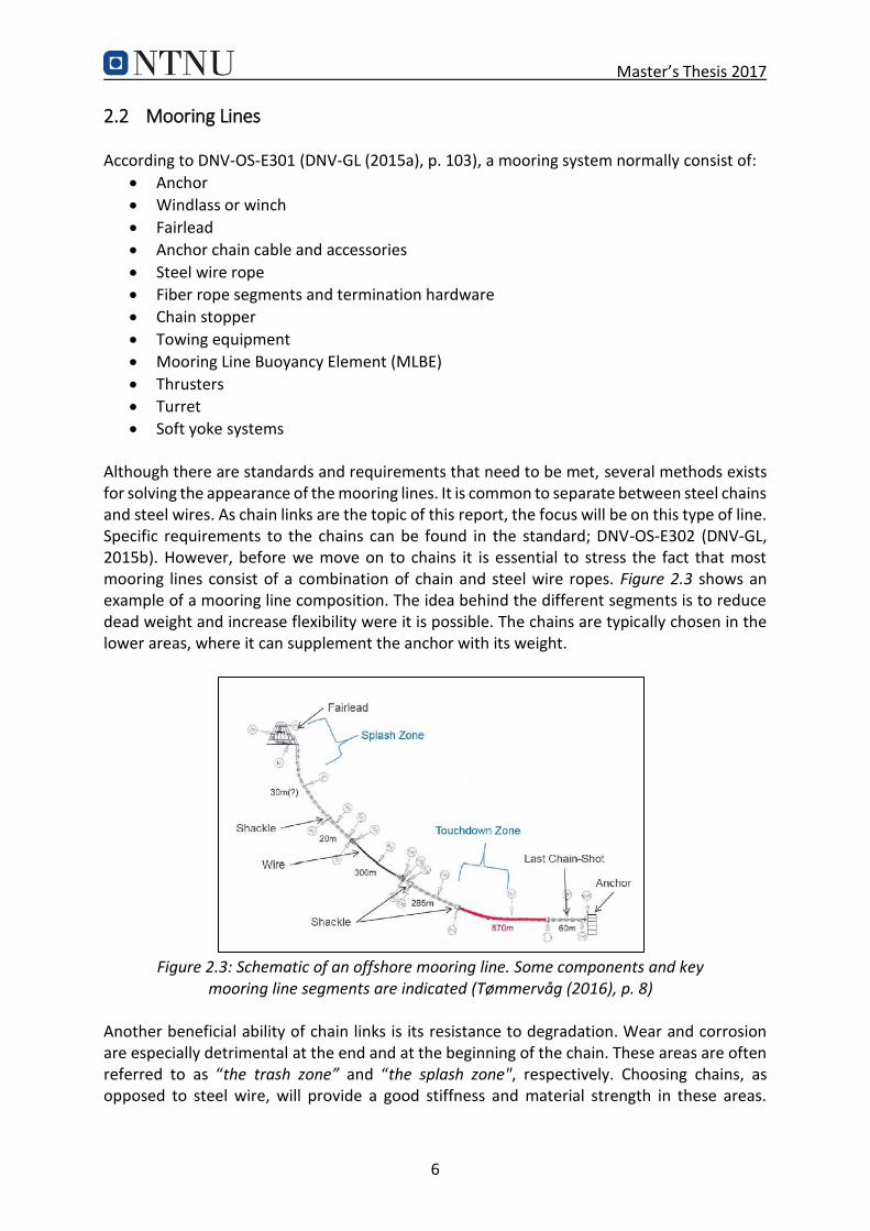
Soft yoke systems Although there are standards and requirements that need to be met, several methods exists for solving the appearance of the mooring lines. It is common to separate between steel chains and steel wires. As chain links are the topic of this report, the focus will be on this type of line. Specific requirements to the chains can be found in the standard; DNV-OS-E302 (DNV-GL, 2015b). However, before we move on to chains it is essential to stress the fact that most mooring lines consist of a combination of chain and steel wire ropes. Figure 2.3 shows an example of a mooring line composition. The idea behind the different segments is to reduce dead weight and increase flexibility were it is possible. The chains are typically chosen in the lower areas, where it can supplement the anchor with its weight.
Figure 2.3: Schematic of an offshore mooring line. Some components and key mooring line segments are indicated (Tømmervåg (2016), p. 8)
Another beneficial ability of chain links is its resistance to degradation. Wear and corrosion are especially detrimental at the end and at the beginning of the chain. These areas are often referred to as “the trash zone” and “the splash zone", respectively. Choosing chains, as opposed to steel wire, will provide a good stiffness and material strength in these areas.
Master’s Thesis 2017
7
However, after some adequate amount of time, there will still be some degradation present, even in the chains. To be appropriate, the steel need to satisfy special requirements. In the offshore industry, five different grades of steel chains are normally used. These grades are listed with their minimum mechanical properties in Table 2.1. Many precautions need to be made before a material is chosen. It is neither desirable to have too low or too high tensile strength. Too low might not be strong enough, while chains with too high tensile strength seem to be more susceptible to hydrogen assisted cracking (Kvitrud, 2014). Consequently, Statoil ASA does not use a higher steel grade than R4S in their structures. (Hove et al., 2015) Table 2.1: Minimum mechanical properties of offshore steel grades (DNV-GL, 2015b)
Steel grade Yield stress [MPa] Tensile strength [MPa]
Elongation [%] Reduction of area [%]
R3 410 690 17 50
R3S 490 770 15 50
R4 580 860 12 50
R4S 700 960 12 50
R5 760 1000 12 50
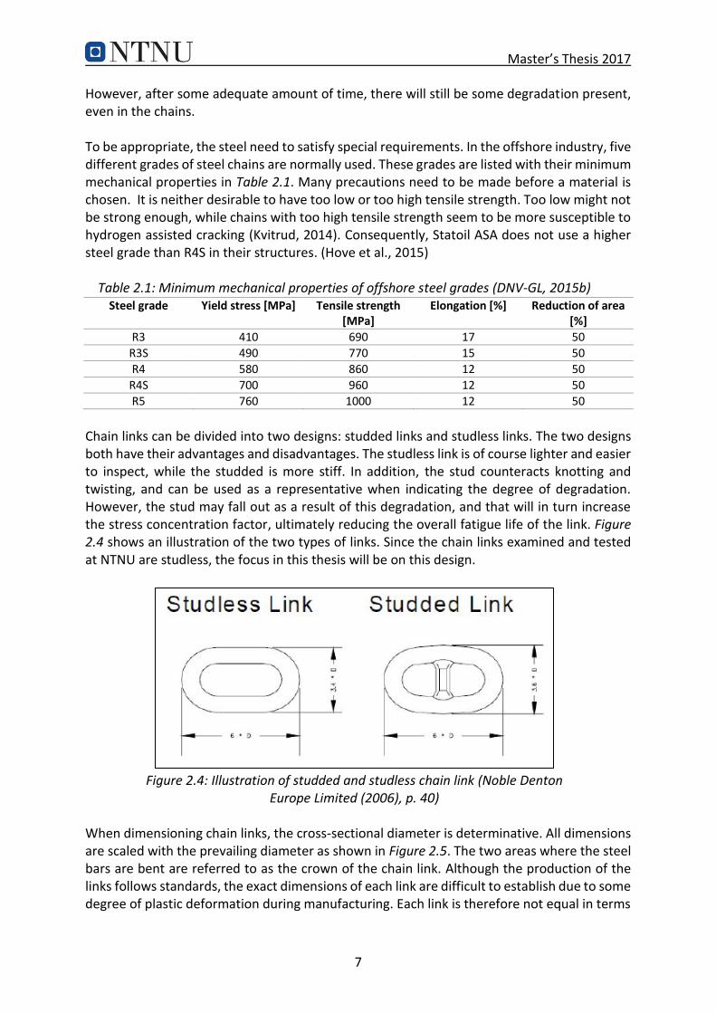
Chain links can be divided into two designs: studded links and studless links. The two designs both have their advantages and disadvantages. The studless link is of course lighter and easier to inspect, while the studded is more stiff. In addition, the stud counteracts knotting and twisting, and can be used as a representative when indicating the degree of degradation. However, the stud may fall out as a result of this degradation, and that will in turn increase the stress concentration factor, ultimately reducing the overall fatigue life of the link. Figure 2.4 shows an illustration of the two types of links. Since the chain links examined and tested at NTNU are studless, the focus in this thesis will be on this design.
Figure 2.4: Illustration of studded and studless chain link (Noble Denton Europe Limited (2006), p. 40)
When dimensioning chain links, the cross-sectional diameter is determinative. All dimensions are scaled with the prevailing diameter as shown in Figure 2.5. The two areas where the steel bars are bent are referred to as the crown of the chain link. Although the production of the links follows standards, the exact dimensions of each link are difficult to establish due to some degree of plastic deformation during manufacturing. Each link is therefore not equal in terms
Master’s Thesis 2017
8
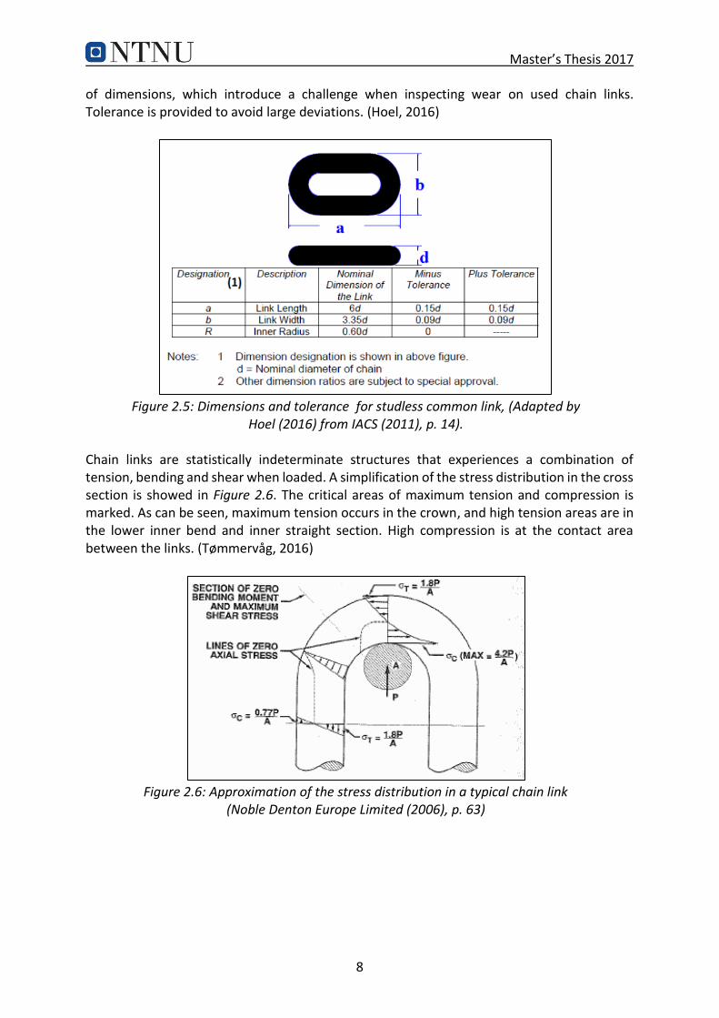
of dimensions, which introduce a challenge when inspecting wear on used chain links. Tolerance is provided to avoid large deviations. (Hoel, 2016)
Figure 2.5: Dimensions and tolerance for studless common link, (Adapted by Hoel (2016) from IACS (2011), p. 14).
Chain links are statistically indeterminate structures that experiences a combination of tension, bending and shear when loaded. A simplification of the stress distribution in the cross section is showed in Figure 2.6. The critical areas of maximum tension and compression is marked. As can be seen, maximum tension occurs in the crown, and high tension areas are in the lower inner bend and inner straight section. High compression is at the contact area between the links. (Tømmervåg, 2016)
Figure 2.6: Approximation of the stress distribution in a typical chain link (Noble Denton Europe Limited (2006), p. 63)

Master’s Thesis 2017
9
2.3 Mooring Failure The failure of a mooring line can be a quite dramatic incident. Even though most structures are designed to tolerate one single line failure, such failures may introduce considerable loss in costs and time. More dramatically, a single failure could eventually develop into a multiple line failure, due to increased loads on the remaining lines. This will not only be an economical drawback – human lives may even be put in danger. Current regulations state that flotels and production facilities should tolerate loss of two lines without serious consequences. The corresponding requirement for mobile drilling facilities is loss of one line without serious consequences (Petroleum Safety Authority Norway (2016c), p. 28). This means that the operator may have the opportunity to continue operation, if the environmental conditions allows it. A common procedure is to analyze the event of line breakage, in order to find which weather conditions that require shut down. If the production or drilling operations are shut down, the consequences of additional line breakage could be reduced, and in such cases lower safety factors than during state of operation is allowed. (Norwegian Maritime Authority (2009), Petroleum Safety Authority Norway (2016a), §3, Petroleum Safety Authority Norway (2015), §63)
2.3.1 A Financial Perspective The financial cost of mooring failure has historically shown to be quite high. Not only does the equipment need to be replaced, it is often required to stop production when waiting for new equipment. In the incident with Gryphon Alpha, the approximate insurance cost was in the range of 440 million GBP as the risers ruptured due to loss of position in a storm. In this accident a FPSO broke four of its ten mooring lines (Crighton, 2013). This was a particularly expensive case, but it gives a perspective of how severe the costs may become. A Joint Industry Project (JIP) was carried out by Noble Denton between 2003 and 2004, aiming to improve the integrity of the mooring system on Floating Production Systems (FPSs). This report investigated the so called business interruption impact in the event of failure and replacement of one line. A hypothetical scenario was introduced for both a medium sized North Sea FPSO, with the capacity of producing 50 000 barrels per day (bpd) and a large West African FPSO, with the capacity of 250 000 bpd. Assuming two days stop in production and necessary safety measures, the final cost came to approximately 2 million GBP for the North Sea FPSO, without including costs for replacing the equipment. The similar assumptions for the West African FPSO, resulted in a loss of almost 10.5 million GBP, due to bigger capacity and longer mobilization time. Even though the cost estimates presented involve a substantial uncertainty, this clearly illustrates that mooring line failure is a great economic burden. (Noble Denton Europe Limited, 2006)
2.3.2 Failure Statistics The rest of this section will introduce some failure statistics on the Norwegian Continental Shelf (NCS). This is included to illustrate the extent of the problem. The statistics are based on reports made by the Petroleum Safety Authority Norway (PSA). In the period 1996-2005, a high number mooring failures were observed on the NCS. The industry took measurements as a result, evidenced by a decrease in incidents the following

Master’s Thesis 2017
10
years. In 2010 the trend shifted, recognized by a period of increase in incidents. As a result, the industry was posed with further questions of improvement measures. Some of the old failure modes had vanished, while others reappeared or were entirely new (Kvitrud, 2014). In total, 16 failures of offshore mooring lines occurred in the period of 2010-2014 on the Norwegian Continental Shelf. The failures were caused by a mixture of overload, fatigue, mechanical damages and gross errors during the manufacturing. PSAs conclusion states that once again a lift of the quality in the industry is needed. In PSAs most recent version of RNNP, at the time of writing, statistics concerning mooring systems between 2000 and 2015 are presented (Petroleum Safety Authority Norway (2016b), p. 125). Figure 2.7 displays number of recorded incidents where mooring lines have lost their load carrying capacity. The incidents are sorted after the number of failed lines. Blue columns demonstrate situations where one line has lost its load carrying capacity, while the red columns represent the same for multiple lines.
Figure 2.7: Number of recorded incidents where mooring lines have lost their load carrying capacity (adapted by author from Petroleum Safety Authority Norway
(2016b), p. 125).
To investigate the occurrence of later failures, the author has been in contact with the PSA. After the incident in 2014, there has only been one failure on the Norwegian Continental Shelf. This happened the 16th of March 2016, on the semi-submersible, Songa Delta (Songa Offshore, 2016). Regarding the statistics, it is reasonable to assume that increased attention has led to less failures. The industry has been more aware of the problem and the PSA has run more frequent supervisions. Although this trend is positive, it does not entirely solve the problem. Means for a proper understanding of the failure mechanisms are still not in place. A substantial amount of time and cost could be saved through more specific methods of locating critical chain segments.
0
1
2
3
4
5
6
7
20
00
20
01
20
02
20
03
20
04
20
05
20
06
20
07
20
08
20
09
20
10
20
11
20
12
20
13
20
14
20
15
Nu
mb
er o
f in
cid
ents
Loss of one line Loss of multiple lines

Master’s Thesis 2017
11
2.4 Inspection Today On the Norwegian Continental Shelf, the requirements for mooring line inspection is a combination of standards and government regulations, (DNV-GL (2015c), p. 133) (Norwegian Maritime Authority (2009), §15). Chains that are less than 20 years, have proper documentation and service history, and no previous failures, should be examined as follows:
100% visual examination
5% non-destructive testing (NDT) on general chain
20% NDT on chain which has been in way of fairleads over the last 5 years
20% NDT on chain that will be in way of fairleads for the next 5 years Typical examples of NDT are magnetic particle inspection (MPI) and liquid penetrant testing (LPI). If no documentation or history is available, the examination shall be increased to include mechanical testing of each length of chain and NDT increased to cover 20% of the whole chain. Chains that are more than 20 years have to be recertified every 2.5 years by the use of NDT on the entire chain length. Although many lines theoretically could be used for 20 plus years, many companies choose to change them more frequently. This is done as a precautionary measure to avoid the catastrophic consequences of mooring line failures. Introduction of a reliable method for determining the fatigue life, could therefore be beneficial both for decreasing number of failures and number of unnecessary replacements.
Master’s Thesis 2017
12
3 Fatigue This chapter will introduce the concept of fatigue and ways of assessing the fatigue life of a component. Towards the end, some important factors influencing the fatigue life will be presented.
3.1 The Basics of Fatigue The process of damage and failure due to cyclic loading is called fatigue. Use of this term arose because it appeared to early investigators that cyclic stresses caused gradual, but not readily observable, change in the ability of the material to resist stress. In fact, today the majority of engineering failures are caused by fatigue. Generally, the fatigue process is initiated by a crack in the material, which slowly disintegrates the material until complete failure occurs. Cracks may initially be present in a component from manufacturing, or they may start early in the service life. Emphasis must then be placed on the possible growth of these cracks by fatigue, as this can lead to brittle or ductile fractures once the cracks are sufficiently large. (Dowling, 2013) The fatigue lives is traditionally divided into two different periods; crack initiation- (𝑁𝑖) and crack propagation period (𝑁𝑝) (Hove, 2016). The initiation of a crack is described to occur due
to movement of slip planes. They will move relative to each other, resulting in multiple inclusions and extrusions, which in turn can result in a crack. Cracks can also initiate at internal impurities in the material.
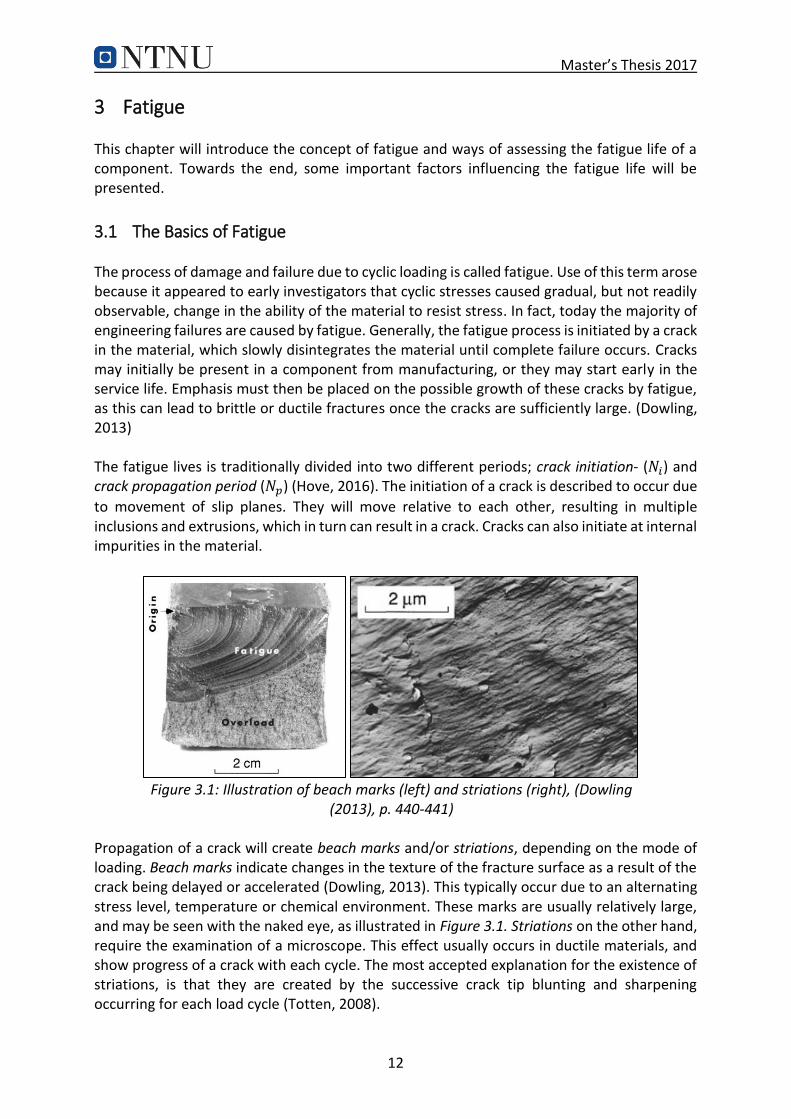
Figure 3.1: Illustration of beach marks (left) and striations (right), (Dowling (2013), p. 440-441)
Propagation of a crack will create beach marks and/or striations, depending on the mode of loading. Beach marks indicate changes in the texture of the fracture surface as a result of the crack being delayed or accelerated (Dowling, 2013). This typically occur due to an alternating stress level, temperature or chemical environment. These marks are usually relatively large, and may be seen with the naked eye, as illustrated in Figure 3.1. Striations on the other hand, require the examination of a microscope. This effect usually occurs in ductile materials, and show progress of a crack with each cycle. The most accepted explanation for the existence of striations, is that they are created by the successive crack tip blunting and sharpening occurring for each load cycle (Totten, 2008).

Master’s Thesis 2017
13
3.2 Fatigue Life Curves An important concept when considering fatigue, is the fatigue life curves. The German scientist, August Wöhler, began the development of design strategies for avoiding fatigue failure, and tested iron, steel, and other metals under bending, torsion and axial loads (Dowling, 2013). Later, by the use of this test data, Basquin formulated Basquin’s law, which shows a logarithmic relation between the stress amplitude applied to the component and its life (Ås, 2006): 𝜎𝑎 = 𝐶 ∙ 𝑁𝑚 (3.1)
Where 𝑁 is cycles to failure, 𝜎𝑎 is the stress amplitude, and 𝐶 and 𝑚 are fitting constants. The use of Stress-Life curves (S-N curves), is today an important part of the fatigue life estimation. The most common form of Eq. (3.1) is: 𝜎𝑎 = 𝜎𝑓
′(2𝑁)𝑏 (3.2)
Where 𝜎𝑓
′ is the fatigue strength coefficient and 𝑏 is the fatigue strength exponent. These
values are usually tabulated are material properties (Dowling, 2013). Basquin’s law is only valid in the high cycle fatigue region, which will be explained next.
Figure 3.2: Fatigue life regions (Hove (2016), p. 16)
The fatigue effects on a component is usually divided into low cycle- and high cycle fatigue. Low cycle fatigue occurs when the component is subjected to large stresses, and life is less than 103 cycles. High cycle fatigue is in the region between 103 to 106 cycles. When a given stress level results in lifetimes beyond 106, the stress is said to be below fatigue limit. Any amount of cycles in this region, does not reduce the life of the component. When the component is subjected to environmental effects, such as corrosion, a fatigue limit does not necessarily exist. In these cases, the stress-life curve will instead show a bend beyond where the material would usually exhibit a fatigue limit.

Master’s Thesis 2017
14
3.3 Assessment of Fatigue There are three major approaches for analyzing and designing against fatigue failures (Dowling, 2013):
Stress-Based approach
Strain-Based approach
Fracture mechanics approach The stress-based approach, focuses on nominal stresses, and considers the effects of mean stress and stress increasing effects, such as notches and grooves. The method is commonly associated with the high cycle fatigue, and thus small elastic deformations. The strain-based approach involves a more detailed analysis of the localized yielding around stress raisers which may occur during cyclic loading. This method is conversely associated with low cycle fatigue. The fracture mechanics approach treats the fatigue failure as a consequence of growing cracks, and analyzes them by the use of fracture mechanics. This situation does not involve the situations before a small crack is developed. After several years of use, a mooring line may suddenly fail due to fatigue. At this point, the line would have experienced a substantial amount of stress cycles, often below the designed fatigue limit. However, as the lines are subjected to a variety of environmental effects, these fatigue limits do not necessarily exist. Corrosion and other mechanisms will lower the curve, hence accelerating the crack initiation. Still, it is assumed that fatigue failure of mooring lines occurs in the region of high cycle fatigue. Consequently, this thesis focuses on the stress-based approach. This method is revolved around the use of S-N curves in order to determine the fatigue life of a component. S-N curves are generated empirically, by testing small specimens until failure, and thus acquire data for applied stress and lifetime. Data for such curves, have over the years, been gathered and established for different components and geometries, and are today listed in standards and recommended practices like DNV RP-C203 (DNV-GL, 2014). The stress-based approach uses relevant S-N curves to determine fatigue properties of a component. These properties are often based on standard specimens that do not necessarily resemble the actual component, and empirical correction factors must therefore often be applied. To properly represent the applied stress in the component, the following formula is used: 𝜎𝑙𝑜𝑐𝑎𝑙 = 𝑆𝐶𝐹𝜎𝑛𝑜𝑚 (3.3)
The fatigue life is affected by numerous factors, which all will result in variations between different specimens of the same material. The author has summarized some of the best documented factors in three categories:
The type of loading
The effect of notches
The surface condition These three factors are explained in detail in the final sections of this chapter.

Master’s Thesis 2017
15
3.4 Type of Loading The fatigue life of a component varies with the loading it is subjected to, that being axial, torsional or bending. However, it is not wholly dependent on the stress amplitude, but also varies with the mean stress applied. Different models to account for this effect has been proposed, such as the one by Morrow: 𝜎𝑎
𝜎𝑎𝑟+
𝜎𝑚𝜎𝑓′ = 1 (3.4)
Where 𝜎𝑎𝑟 is the equivalent zero mean stress amplitude, and 𝜎𝑚 is the applied mean stress. The mean stress is given by
𝜎𝑚 =𝜎𝑚𝑎𝑥 +𝜎𝑚𝑖𝑛
2
(3.5)
Where 𝜎𝑚𝑖𝑛 is the minimum stress for a cycle and 𝜎𝑚𝑎𝑥 is the maximum stress. When running fatigue tests at different stress ranges, the mean stress is commonly expressed by the load ratio 𝑅 =
𝜎𝑚𝑖𝑛
𝜎𝑚𝑎𝑥 (3.6)
So that 𝑅 = −1 for zero mean stress. If the mean stress is above zero, like in Figure 3.3, R becomes value between 0 and 1.
Figure 3.3: Constant amplitude cycling with nonzero mean stress 𝜎𝑚 (Dowling (2013), p. 419)

Master’s Thesis 2017
16
3.5 Stress Concentration Factors To understand the notch effect, it is essential to introduce the concept of stress concentration. A stress concentration is a location in a specimen where the stress is concentrated. This occurs due to discontinuities in the material, which interrupt the stress pattern in the specimen, making it non-uniform, hence increasing the local stress level. The presence of shoulders, grooves, holes and pits are some examples. The measure of the concentration is denoted by the stress concentration factor (SCF). This factor is defined as ratio between the peak stress and a relevant reference stress, and it is formulated as follows (Pilkey, 1997): 𝐾𝑡 =
𝜎𝑚𝑎𝑥
𝜎𝑛𝑜𝑚 (3.7)
𝐾𝑡𝑠 =
𝜏𝑚𝑎𝑥
𝜏𝑛𝑜𝑚 (3.8)
Here, 𝐾𝑡 represent the normal stress (tension or bending) and 𝐾𝑡𝑠 the shear stress (torsion). The maximum stress in the member is given by, 𝜎𝑚𝑎𝑥 and 𝜏𝑚𝑎𝑥, while 𝜎𝑛𝑜𝑚 and 𝜏𝑛𝑜𝑚 is a measure of the reference normal- and shear stress. The t subscript indicates that the stress concentration factor is a theoretical factor. It is important to note that 𝐾𝑡 is most relevant to ideal elastic materials under dynamic loading, and is mainly dependent on geometry and load type. The reference stress is commonly recognized as the nominal stress, which is a stress that depends on the problem at hand. Two methods exist for defining these stresses, and they are explained and discussed through the example in Figure 3.4.
Figure 3.4: Tension bar with circular hole (Pilkey (1997), p.7)
By using the stress in a cross section far from the circular hole as the reference stress, the SCF can be define as 𝐾𝑡𝑔, where g stands for gross cross-sectional area. Thus, the nominal stress
is defined by;
𝜎𝑛𝑜𝑚 = 𝑃
𝐻ℎ= 𝜎
(3.9)

Master’s Thesis 2017
17
Thus, the stress concentration factor becomes;
𝐾𝑡𝑔 = 𝜎𝑚𝑎𝑥
𝜎𝑛𝑜𝑚=
𝜎𝑚𝑎𝑥
𝜎=
𝜎𝑚𝑎𝑥𝐻ℎ
𝑃
(3.10)
On the other hand, if one defines the reference stress based on the cross section at the hole, which is formed by removing the circular hole from the gross cross section, then the SCF will be defined by 𝐾𝑡𝑛, where n stands for net cross-sectional area. If the stresses at this cross section are uniformly distributed they can be formulated as:
𝜎𝑛 =𝑃
(𝐻 − 𝑑)ℎ
(3.11)
Where 𝐻 is the width of the plate, and ℎ is the thickness. Thus the stress concentration based on the reference stress, 𝜎𝑛, is defined by:
𝐾𝑡𝑛 = 𝜎𝑚𝑎𝑥
𝜎𝑛𝑜𝑚=
𝜎𝑚𝑎𝑥
𝜎𝑛=
𝜎𝑚𝑎𝑥(𝐻 − 𝑑)ℎ
𝑃= 𝐾𝑡𝑔
𝐻 − 𝑑
𝑃
(3.12)
There are no distinct rules for which of these concentration factors to use, the choice is entirely up to the user. As long as the appropriate reference stress is used, the final solutions will be identical. However, one could argue that 𝐾𝑡𝑔 is easier to determine as 𝜎 immediatley
is evident from the geometry of the bar. On the other hand, if the values are taken from a
chart, 𝐾𝑡𝑔 will be harder to determine when 𝑑
𝐻> 0.5, since the curves in these areas become
very steep. For that particular use, 𝐾𝑡𝑛 is superior. The most important thing is however to indicate which one that has been used.
3.5.1 Stress Concentration Factors as a Three-Dimensional Problem The stress concentration factor is mainly dependent on geometry and loading. Still, when introducing three-dimensional problems, some additional factors may be influential. The current section discusses the Poisson’s ratio, and takes a look at how this ratio can alter the stress distribution. It is a parameter that often is involved in three-dimensional stress concentration analyses, the influence will vary with the configuration of the problem. Consider a hyperbolic circumferential groove in a round bar under tension load P, see Figure 3.5. The stress concentration factor in the axial direction is;
𝐾𝑡𝑥 =𝜎𝑥𝑚𝑎𝑥
𝜎𝑛𝑜𝑚=
1
(𝑎𝑟) + 2𝜈𝐶 + 2
[𝑎
𝑟(𝐶 + 𝜈 + 0.5) + (1 + 𝜈)(𝐶 + 1)]
(3.13)
Whereas in the circumferential direction;
𝐾𝑡𝜃 =𝜎𝜃𝑚𝑎𝑥
𝜎𝑛𝑜𝑚=
𝑎𝑟
(𝑎𝑟) + 2𝜈𝐶 + 2
(𝜈𝐶 + 0.5) (3.14)

Master’s Thesis 2017
18
From this it is obvious that the two functions are dependent on𝜈. As 𝜈 increases, 𝐾𝑡𝑥 will decrease slowly, whereas 𝐾𝑡𝜃 increases relatively rapidly. Consequently, the Poisson’s ratio may actually play a significant role on how the stresses are distributed. Steels usually have Poisson’s ratios between 0.27 and 0.3, hence it does not require significant changes before the material transforms substantially. Still, it is important to be aware of the effect these
properties may have. In both of the above equations, 𝐶 is substituted for √(𝑎/𝑟) + 1.
Figure 3.5: Hyperbolic circumferential groove in a round bar (Pilkey (1997), p.12)
The example above shows that even for very simple load conditions, as uniaxial tension P, a biaxial system may be the result. The axial load P results in an axial tension 𝜎𝑥 = 𝜎1 and a circumferential tension 𝜎𝜃 = 𝜎2, which could be expressed in principal stresses. A principal stress is the normal stress 𝜎 acting on an area 𝐴, when 𝐴 is free of shear stress (Young and Cook, 1999). Considering a three-dimensional problem, there are three principal stresses; one is the maximum normal stress acting on any plane, another is the minimum normal stress acting on any plane, and the remaining one has an intermediate value. Any state of stress can be reduced through a rotation of coordinates to a state of stress involving only the principal stresses 𝜎1, 𝜎2 and 𝜎3. If a member is in an uniaxial stress state (i.e., 𝜎𝑚𝑎𝑥 =𝜎1, 𝜎2 =𝜎3 = 0), the maximum stress can be used directly in Eq. (3.7) for a failure analysis. However, when the location of the maximum stress is in a biaxial or triaxial stress state, the case is a bit different. Then, it is important to consider not only the effects of 𝜎1, but also 𝜎2 and 𝜎3. This is taken from the theories of strength and failure. The most used theory is the von Mises theory. The following expression was proposed by Richard von Mises (1913), as representing a criterion of failure by yielding:
𝜎𝑦 =√(𝜎1 − 𝜎2)2 +(𝜎2 − 𝜎3)2 + (𝜎1 − 𝜎3)2
2
(3.15)

Master’s Thesis 2017
19
Where 𝜎𝑦 is the yield strength in a uniaxial loaded bar. The quantity on the right-hand side of
Eq. (3.15), which is sometimes available as output of structural analysis software, is often referred to as the equivalent stress 𝜎𝑒𝑞:
𝜎𝑒𝑞 =√(𝜎1 − 𝜎2)2 + (𝜎2 − 𝜎3)2 + (𝜎1 − 𝜎3)2
2
(3.16)
To combine the stress concentration and the von Mises theory, introduce a factor 𝐾𝑡
′: 𝐾𝑡
′ = 𝜎𝑒𝑞
𝜎 (3.17)
In general, 𝐾𝑡
′ is about 90% to 95% of 𝐾𝑡 and not less than 85%. As 𝐾𝑡′ is lower than and quite
close to 𝐾𝑡, it can be concluded that the usual design using 𝐾𝑡 is on the safe side and will not be accompanied by significant errors. Therefore most charts are based on 𝐾𝑡.
3.5.2 Notch Sensitivity Thus far, this paper has only dealt with the theoretical stress concentration factor. This factor applies mainly to ideal elastic materials and depend on the geometry of the body and the loading. Sometimes, it is however preferable to use a more realistic model. When the applied loads reach a certain level, plastic deformations may be involved. Thus, the actual strength of the structural members may be quite different from that derived using theoretical stress concentration factors, especially for the cases of impact and alternating loads. As a consequence, it is reasonable to introduce a new concept, namely the effective stress concentration factor, 𝐾𝑒. This factor is obtained experimentally, and is not only a function of the geometry but also of material properties. (Pilkey, 1997) The effective stress concentration factor can be defined by the example in Figure 3.6. Here, there are two specimens with the same material, one has a rupture load, while the other has 𝑃, the diameter 𝑑 is identical. Then the effective stress concentration factor becomes:
𝐾𝑒 =𝑃
𝑃′
(3.18)
Figure 3.6: Specimens for obtaining 𝐾𝑒 (Pilkey (1997), p.36)

Master’s Thesis 2017
20
As the factor is dependent on the material properties, the effect will be different in ductile and brittle specimens. Let us now consider the effects of 𝐾𝑒 in a ductile material. We choose to look at the two tensile specimens in Figure 3.6 once again. If the maximum stress at the root of the notch is less than the yield strength 𝜎𝑚𝑎𝑥 =𝜎𝑦, the stress distribution near the notch would appear as in curve
1 and 2 in Figure 3.7. The maximum stress value is: 𝜎𝑚𝑎𝑥 = 𝐾𝑡𝜎𝑛𝑜𝑚 (3.19)
As the 𝜎𝑚𝑎𝑥 exceeds 𝜎𝑦, the strain at the root of the notch continues to increase but the
maximum stress increases only slightly. The stress distribution on the cross section will be of the form of curves 3 and 4 in Figure 3.7, and hence Eq. (3.19) no longer applies to this case. As 𝜎𝑛𝑜𝑚 continues to increase, the stress distribution at the notch becomes more uniform and the effective stress concentration factor 𝐾𝑒 is close to unity.
Figure 3.7: Stress distribution near a notch for a ductile material (Pilkey (1997), p.37)
It can be reasoned that the effective stress concentration factor depends on the characteristics of the material and the nature of the load, as well as the geometry of the stress raiser. The maximum stress at the rupture can be defined to be: 𝜎𝑚𝑎𝑥 = 𝐾𝑒𝜎𝑛𝑜𝑚 (3.20)
To express the relationship between 𝐾𝑒 and 𝐾𝑡, introduce the concept of notch sensitivity 𝑞:
𝑞 = 𝐾𝑒 − 1
𝐾𝑡 − 1
(3.21)
Master’s Thesis 2017
21
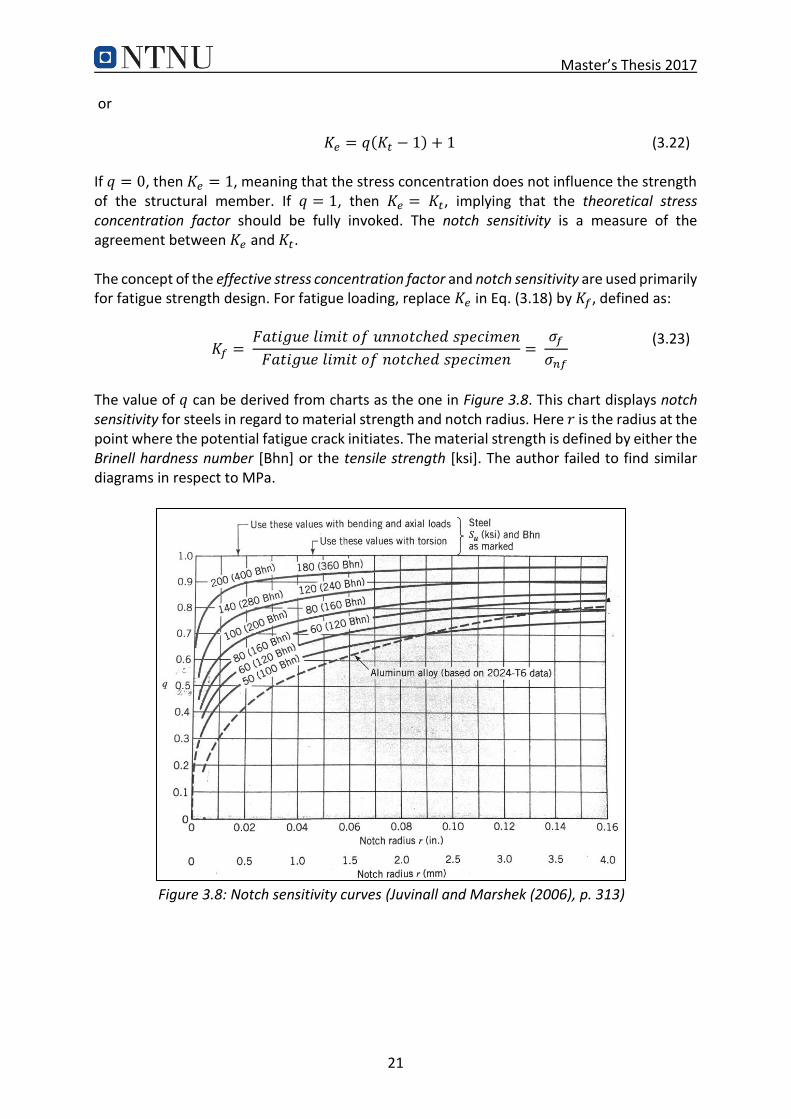
or 𝐾𝑒 = 𝑞(𝐾𝑡 − 1) + 1 (3.22)
If 𝑞 = 0, then 𝐾𝑒 = 1, meaning that the stress concentration does not influence the strength of the structural member. If 𝑞 = 1, then 𝐾𝑒 =𝐾𝑡, implying that the theoretical stress concentration factor should be fully invoked. The notch sensitivity is a measure of the agreement between 𝐾𝑒 and 𝐾𝑡. The concept of the effective stress concentration factor and notch sensitivity are used primarily for fatigue strength design. For fatigue loading, replace 𝐾𝑒 in Eq. (3.18) by 𝐾𝑓, defined as:
𝐾𝑓 = 𝐹𝑎𝑡𝑖𝑔𝑢𝑒𝑙𝑖𝑚𝑖𝑡𝑜𝑓𝑢𝑛𝑛𝑜𝑡𝑐ℎ𝑒𝑑𝑠𝑝𝑒𝑐𝑖𝑚𝑒𝑛
𝐹𝑎𝑡𝑖𝑔𝑢𝑒𝑙𝑖𝑚𝑖𝑡𝑜𝑓𝑛𝑜𝑡𝑐ℎ𝑒𝑑𝑠𝑝𝑒𝑐𝑖𝑚𝑒𝑛=
𝜎𝑓
𝜎𝑛𝑓
(3.23)
The value of 𝑞 can be derived from charts as the one in Figure 3.8. This chart displays notch sensitivity for steels in regard to material strength and notch radius. Here 𝑟 is the radius at the point where the potential fatigue crack initiates. The material strength is defined by either the Brinell hardness number [Bhn] or the tensile strength [ksi]. The author failed to find similar diagrams in respect to MPa.
Figure 3.8: Notch sensitivity curves (Juvinall and Marshek (2006), p. 313)

Master’s Thesis 2017
22
3.6 Surface Conditions The surface condition of the chains has shown to be a result of several degradation mechanisms, often working together. The most detrimental seem to be wear, corrosion and environmental assisted cracking (EAC). This thesis will not go in detail on these mechanisms, instead it will focus on the effect of them. For a detailed explanation of the degradation mechanisms the reader is referred to Tømmervåg (2016). As fatigue cracks initiate predominantly at the free surface of a material, the condition of the surface can be assumed to be critical with regard to fatigue crack initiation (Suhr, 1986). It is common practice to use three parameters when referring to the surface conditions (Ås, 2006):
A geometrical parameter; surface roughness
A mechanical parameter; residual stress
A metallurgical parameter; microstructure These parameters can vary separately according to the machining- or service conditions. In engineering design, the effects of these parameters are commonly accounted for by using empirical reduction factors which modify the fatigue limit of the material: Δσ𝑚𝑜𝑑 = 𝐶𝑠Δσ0 (3.24)
where 𝐶𝑠 is the product of individual surface reduction factors for residual stress, surface roughness and microstructure. The fatigue limit is commonly taken at 𝑁𝑓 = 107 cycles. These
factors are almost impossible to quantify with any degree of confidence, so we tend to present data in terms of the measurable surface roughness and the method of manufacturing, see Figure 3.9. Each curve in Figure 3.9 is based on fatigue limit testing of several steel types.
Figure 3.9: Effect of surface condition on fatigue limit for steels with various manufacturing methods and hardness (Juvinall and Marshek (2006), p. 301)

Master’s Thesis 2017
23
Surface roughness covers a wide dimensional range, extending from that produced in the largest planing machines having a traverse step of 20 mm or so, down to the finest lapping where the scratch marks may be spaced by a few tenths of a micrometer (Whitehouse (1994), p. 7). In the case of the mooring chains, it is relevant to divide into a measure of the entire surface, taking pits and everything into account, and a measure for the local surface, outside and inside of the pits. Regardless of the measure, these values impose stress concentrations in the surface where fatigue cracks may initiate. Residual stress is introduced through machining- and thermal processes. Material removal can cause the outer material layer to yield in tension, producing compressive residual stresses at the surface due to the constraint of the bulk material. Residual stresses are also affected by thermal processes such as heat treatment and welding. Compressive residual stress is beneficial while tensile residual stress is detrimental to fatigue life. (Ås, 2006) Even the surface microstructure may include stress raisers. This can come from inclusions and second phase particles with different elastic modulus than the surrounding matrix. This introduce a “weakest-link” mechanism in the specimen – the larger the specimen, the larger is the probability of encountering microstructural weaknesses. Consequently, a reduction of fatigue life can be observed with the increase in specimen size. (Ås, 2006) Not all parameters are distinguishable through the application of a 3D-scanner. Therefore, the focus of this thesis, will mainly be on the severe corrosion pits, for whom we have good tools for capturing. In addition, a small study will be conducted to see if the existing tools may provide reasonable values for the surface roughness.

Master’s Thesis 2017
24
3.7 FEA and Fatigue Life Assessment This thesis aims to use finite element analysis (FEA) for the prediction of cycles to failure. The idea behind this procedure is taken from Eq. (3.1), which states that the local stress is a product of the nominal stress and an appropriate SCF. After defining the maximum local stress, this value can be used in a relevant S-N diagram. This S-N diagram must be based on test specimens that are comparable to the simulated component. Additional correction factors, as the ones discussed in the previous sections, can be added for a more precise evaluation. The reference S-N diagram used in this project, is taken from DNV-RP-C203. These S-N curves are defined by the following formula: 𝑁 = 𝐶(Δσ)𝑚 (3.25)
The stress range Δσ is thus altered by multiplying either stress concentration factors, or other correction factors, i.e. as in Eq. (3.24). The cycles to failure is represented through 𝑁 in the above equation, 𝐶 and 𝑚 are fitting constants, with 𝑚 being the negative slope and 𝐶 the intercept on the 𝑁-axis. The current FEA will only use 𝐾𝑡𝑔, as it would be difficult to always calculate the loss of
material in the evaluated pits. For simplicity, this value will from now on be denoted as 𝐾𝑡. Furthermore, it has been considered most appropriate to use the equivalent stress 𝜎𝑒𝑞 as the
relevant stress parameter, resulting in the theoretical stress concentration factor 𝐾𝑡′. As the
problem is a three-dimensional scenario, Poisson’s ratio is expected to be influential, and consequently von Mises is regarded as the best stress representation. This is further backed by statements in DNV-RP-C203, which states that stress ranges calculated based on von Mises can be used for fatigue of notches in base material where initiation of a fatigue crack is a significant part of the fatigue life (DNV-GL (2014), p. 15).

Master’s Thesis 2017
25
4 Replicating a Surface This chapter will introduce the scanning method used for replicating the actual chain links. Techniques for quantifying the surface parameters will be discussed, before a simple validation study is presented. Finally, the preparation of a relevant fatigue test is described on the basis of scanning procedures and realistic pit geometries.
4.1 3D-scanning The use of 3D-scanners has drastically increased during the last couple of years. Contemporary scanners are accurate and often less complicated in use than traditional measuring methods. Though there are numerous ways to use these scanners, one can still divide the techniques into two main categories; contact and non-contact methods. Contact methods typically use a probe to trace the surface of the measuring object, while non-contact uses lights or lasers. The scanner used throughout this project exploits the non-contact method, and the following section will give a brief introduction to how this scanner is used. (Bache, 2016)
4.1.1 ATOS
Figure 4.1: Configuration of ATOS III SO at the Department of Structural Engineering.
The ATOS III SO is a structured light scanner that projects different fringe patterns onto the measuring object. By the use of triangulation and recording from two cameras, the ATOS can calculate the distance from the object to the scanner. Each camera has a resolution of 2048 pixels, resulting in 4 million data points in one single measurement. By the use of reference points, ATOS transforms these individual measurements automatically into a common global coordinate system. (GOM, 2008, GOM, 2010) Every component that is scanned by the ATOS undergoes several scans in different positions in order to completely capture the geometry. After that is done, the individual scans are stitched into one single surface. In order to create an actual surface that can be exported and analyzed, the surface needs to be polygonised. This is done either manually or automatically in the scanning software. The result is something called a polygon surface. This surface can eventually be exported and analyzed in a wide range of software.

Master’s Thesis 2017
26
After initial creation of a scan, it is common practice to perform certain after-treatments. This often involve deleting of scanner noise, reduction of file size and other surface enhancement tools. These processes have already been studied in detail by Hoel (2016), who prepared a surface enhancing routine for future use in this project. As a consequence, much work is gathered from his thesis. However, as the author discovered certain flaws with the finished surfaces, some additional steps have been added. A brief review of the post-processing steps is thus included in Appendix A. For after-treatments the author has deployed the powerful GeoMagic Studio 14, henceforth referred to as GS14. This is a software created entirely for the processing of surface scans, and thus contains several useful tools. Some of the relevant tools will be discussed in the following, and some in later parts of the thesis. Eventually, when a surface is completely processed, it is ready for meshing, which is the last step before numerical analysis. These processes will however be discussed later in Section 6.3.
4.1.2 Important Limitation with the ATOS Issues with the surface are often the main cause of bad measurements. The surface could be too complex for a specific set of lenses, or it could be too heterogeneous in color distribution. In general, the ATOS system only accepts data if both two cameras are in agreement. This introduces problems when you for instance have strong color transitions or shiny metal areas. The general rule is that a dull and light surface is the optimal surface to scan. The overall project considers a corroded chain surface, which is rather simple to measure. This surface is relatively dull in color, and does not exhibit too strong color transitions. Problems arise however if the surface is substantially scratched, and fresh shiny metal appears. Shiny metal has been a problem in several measurements throughout this work, and the author has thus been forced to establish precautionary measures. The solution to shiny metal areas has shown to be simple white spray paint, with a dull finish. An illustration of the spray and how it has been used, can be seen in the figure below. The small layer of paint that is introduced through spray painting is assumed to be negligible for the result.
Figure 4.2: Illustration of simple white dull spray paint

Master’s Thesis 2017
27
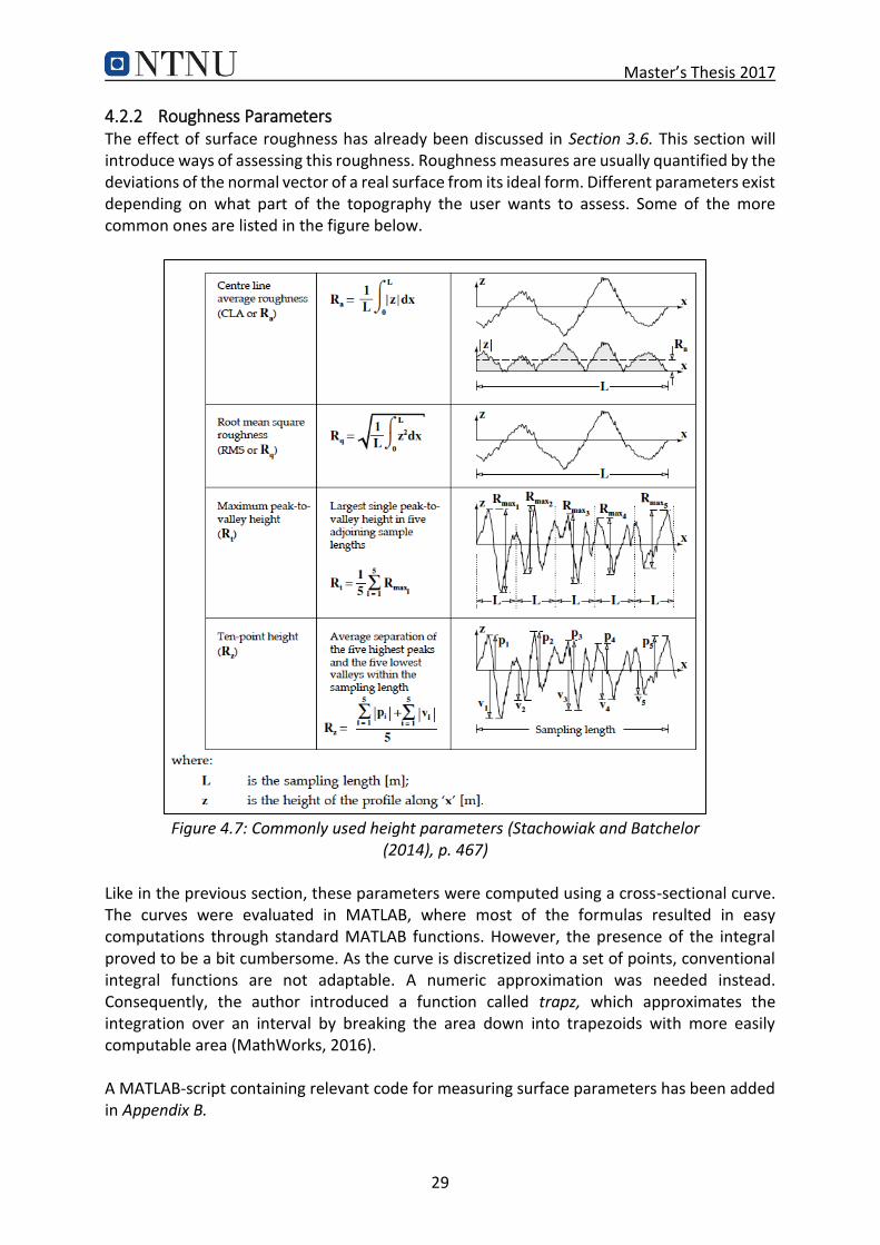
4.2 Extracting Surface Parameters This section will review some methods for extracting surface parameters from the chain links. The parameters are divided in roughness parameters and geometry parameters.
4.2.1 Geometry Parameters The shape of a pit is normally described through its cross section. Several shapes could be defined, with the most common ones defined in Figure 4.3. Even though no exact measures are used for determining the shapes, certain geometries could be useful when separating between them. As a consequence, this section will introduce some simple parameters, referred to as geometry parameters. They consist of simple measures like depth, diameter and curvature.
Figure 4.3: Variations in the cross-sectional shape of pits (ISO (2008), p. 2)
Different possibilities have been investigated when extracting these measurements. The first, and most visual alternative, was to use a direct tool in GS14. This method creates a best-fit plane to a surface, and uses the fitting parameters to evaluate distances from the plane. Though being easy and giving good results for one cavity, it proved more challenging for several pits. When introducing several pits, there was no easy way of distinguishing the values of the different pits. Still, this might be the superior choice when approximate numbers are sufficient, due to the methods simplicity. Figure 4.4 shows an illustration of the procedure.
Figure 4.4: Measuring depth with a best-fit plane

Master’s Thesis 2017
28
Figure 4.5: From surface scan to sample points
The other method investigated was based on creating a cross-sectional curve through the pit, exploiting an option called curve sectioning in GS14. This curve was successively converted into a uniform set of points, that had the ability to be exported, and thus evaluated in an alternate software. As the points were defined in x- and z-directions, they were ideal inputs for software like MATLAB, that easily can determine the lowest point in a large sample. Not only was this used for evaluating the depth, measures like diameter and curvature were also found. An approximation of the curvature was computed at the middle point of three successive points, like the illustration in Figure 4.6 indicates.
Figure 4.6: Radius of curvature
The radius of the curvature, and the curvature itself, was established using the following formulas: 𝑥𝑀 =√𝑟𝜅2 − 2𝑦𝑚𝑦3 − 𝑦32 + 𝑥2 (4.1)
𝑦𝑚 =√𝑟𝜅2 − 2𝑥𝑚𝑥𝑚 − 𝑥12 + 𝑦1 (4.2)
𝑟𝜅 =√𝑥𝑚2 − 2𝑥𝑚𝑥2 +𝑥22 +𝑦𝑚2 − 2𝑦𝑚𝑦2 + 𝑦2
2 (4.3)
𝜅 =1
𝑟𝜅
(4.4)
Here 𝜅 is the curvature and 𝑟𝜅 the radius of the curvature. This is a simple approximation, but still regarded to be appropriate for our use.
Master’s Thesis 2017
29
4.2.2 Roughness Parameters The effect of surface roughness has already been discussed in Section 3.6. This section will introduce ways of assessing this roughness. Roughness measures are usually quantified by the deviations of the normal vector of a real surface from its ideal form. Different parameters exist depending on what part of the topography the user wants to assess. Some of the more common ones are listed in the figure below.
Figure 4.7: Commonly used height parameters (Stachowiak and Batchelor (2014), p. 467)
Like in the previous section, these parameters were computed using a cross-sectional curve. The curves were evaluated in MATLAB, where most of the formulas resulted in easy computations through standard MATLAB functions. However, the presence of the integral proved to be a bit cumbersome. As the curve is discretized into a set of points, conventional integral functions are not adaptable. A numeric approximation was needed instead. Consequently, the author introduced a function called trapz, which approximates the integration over an interval by breaking the area down into trapezoids with more easily computable area (MathWorks, 2016). A MATLAB-script containing relevant code for measuring surface parameters has been added in Appendix B.

Master’s Thesis 2017
30
4.3 Validation Study of Scan Before using actual scans in a finite element analysis, the author wanted to validate the accuracy of the scans. The aim was not necessarily to find a specific number representing the accuracy, but to control that the measurements were in the same ballpark as the actual dimensions. One test was performed for the surface roughness, and one for the overall geometry.
4.3.1 Artificially Made Corrosion Pits The first validation step focused on how well the scanner was able to represent a certain geometry. By making the geometries from scratch, one can decide the dimensions in prior, and eventually use them as reference to the scanned results. For relevance to the mooring chains, the idea was to create something comparable to the large corrosion pits. This was achieved by machining pits in a small metal plate. Two sets of pits were established, one hemispherical and one conical. Both had a diameter of approximately 8 mm, and a depth of 4 mm. The hemispherical ones were made with a milling tool, whereas the conical were made with a drill. To more precisely represent the surface of a corrosion pit, two of each pit category was corroded. This was achieved by introducing simple NaCl-water in the pits, and leaving them over the weekend. The remaining pits were kept uncorroded due to reference purposes. Eventually the scanned pits were measured using the methods in Section 4.2.1. Unfortunately, due to shiny metal the uncorroded pits were unable to be captured. The associated reflection introduced too much trouble for the scanner, and the precautionary measures discussed in Section 4.1.2 were not yet developed.
Figure 4.8: Artificial corrosion pits
Although the dimensions were defined in prior, machining of a component always present some amount of error. For optimizing the accuracy, the author introduced additional measuring procedures. Instead of just comparing with the initial dimensions, the scanner was matched with other scanners and equipment of different accuracy. An illustration of the different equipment can be found in Figure 4.9, on the next page. The equipment existed of two micrometers, a supplementary 3D-scanner, a laser measurement tool and a replicating compound. The replicating compound is spurted in the pits and left there for hardening. When they are firm, the small rubbery pits are sliced and scanned with a traditional paper scanner. Figure 4.9 e) illustrates the hardened pit before slicing. The scanned slices were eventually measured using simple geometry features in

Master’s Thesis 2017
31
Microsoft PowerPoint. The idea was originally to use an optical comparator, but such equipment could not be located.
a) b) c)
d) e) f)
Figure 4.9: Equipment used for measuring depth and diameter of artificial corrosion pits; a) micrometer with pointed ends, b) inside micrometer, c)
ATOS III SO 3D-scanner, d) ROMER RA-7525SI 3D-scanner, e) high resolution replicating compound and f) Panasonic industrial laser HG-C1030-P
All the different equipment has an initial accuracy, which is listed in Table 4.1. However, as most of the measuring procedures introduce a substantial amount of human error, these accuracies are not given too much attention in this study. Instead, they are used as a rough guideline for finding the most accurate tool. If the aim was to make a real statistical validation study, the situation would be different. However, such statistical studies require an abundant amount of measurements, and was not found crucial for the particular work. Table 4.1: Accuracy of the equipment
Equipment Accuracy [mm] Comments
Micrometer with pointed ends
0.005 This tool was initially calibrated with a deviation of 0.12 mm. However, as we subtract the measure of the plate thickness with the thickness of the remaining material in a pit, this deviation eliminates itself. Instead, the accuracy was taken from information written on the tool.
Inside micrometer 0.005 Accuracy taken from information written on the tool.
Panasonic 0.01 Information from Panasonic (2016)
ATOS III SO 0.03-0.08 Information from GOM (2008) and Schuman-Olsen et al. (2010)
ROMER RA-7525SI 0.038 Information from Hexagon Manufacturing Intelligence (2016)
High Resolution Replicating Compound
0.0001 The compound has a resolution of 0.0001 mm (written on the box). The scanning of the pieces will arise some additional error. A standard Ricoh paper scanner was used for digitizing the sliced piece.

Master’s Thesis 2017
32
The micrometer with the pointed end is very exposed to human error, and is therefore not considered the most accurate choice. The same applies for the high resolution compound, which in addition needs to undergo four different procedures; spurting, slicing, scanning and final measuring. Instead, more faith is put in the industrial laser from Panasonic. This device experience a minimal amount of human error and has a good initial accuracy. Hence, this measuring procedure is viewed superior when examining the depth. The ROMER utilize the same measuring methods as the ATOS, but produces the scans in a different way. It is not considered superior to the ATOS. Table 4.2: Depth of pits
Equipment Depth of pits [mm]
2 3 5 6
Micrometer with pointed ends 3.99 4.05 3.89 3.92
Panasonic 4.01 4.03 3.90 3.92
ATOS 4.00 4.04 3.88 3.93
ROMER 4.02 4.02 3.87 3.93
High Resolution Replicating Compound 3.96 4.10 3.90 3.89
The final depth measurements display small deviations between the different procedures, with none drastically off. It can be seen that the ATOS only differ by a couple of hundredth decimal places to the Panasonic. This is viewed as acceptable results, and it is concluded that the ATOS appropriately measure the depths. Unfortunately, the industrial laser is inaccessible for the diameter measurements – the device cannot be used on these kinds of measurements. Instead, the inside micrometer is regarded as the superior tool. Table 4.3: Diameter of pits
Equipment Diameter of pits [mm]
2 3 5 6
Inside micrometer 8.00 8.03 8.01 8.07
ATOS 8.03 8.05 8.04 8.06
ROMER 8.03 7.96 8.09 8.12
High Resolution Replicating Compound 8.11 8.05 8.13 8.05
Also this time, the the ATOS only differ by a couple of hundredths, and we can conclude that the procedure is sufficient for representing a reasonable diameter.
4.3.2 Surface Roughness Specimen The second control scan was taken of a traditional surface roughness specimen. This specimen was chosen for the evaluation of surface roughness. It is a piece with known parameters, as can be seen in Figure 4.10. The value of the surface roughness ranges from 𝑅𝑎 = 50.0𝜇𝑚 to 𝑅𝑎 = 0.4𝜇𝑚. To start with, only the four roughest was scanned. If these scans gave reasonable results, the idea was to move on to the remaining 𝑅𝑎-values.

Master’s Thesis 2017
33
Figure 4.10: Surface roughness specimen
After initial scanning, the surface was post-processed in four different ways. The post-processing routine adopted from Hoel (2016) was already viewed as superior, the only reason for performing several procedures was to control that the finer surfaces maintained their peaks, which could have been mistaken for scanner noise. Table 4.4: Four different post-processing routines
Routine Procedures Comments
Alternative 1 - Convert to points - Point clean-up - Wrapping - Mesh doctor - Relax surface
Exactly the same routine as used in Hoel (2016)
Alternative 2 - Convert to points - Point clean-up - Wrapping - Mesh doctor
Alternative 3 - Convert to points - Point clean-up - Wrapping
Alternative 4 Untreated
The method for computing roughness parameters discussed in Section 4.2.2 was executed on the surface, and results are given in Table 4.5. 𝑅𝑎 has been chosen as the relevant parameter, and the values are measured on the normal of the roughness area, which is the highest point on the curved area. Table 4.5: Surface roughness measurements, 𝑅𝑎 [𝜇𝑚]
Roughness number
Measured on the normal
Alternative 1 Alternative 2 Alternative 3 Alternative 4
N12 52.5 51.5 49.8 59.6 63.0
-> 1.9% off -> 5.1% off -> 13.5% off -> 20.0% off N11 23.8 14.8 14.5 18.8 22.5
-> 37.9% off -> 39.1% off -> 21.0% off -> 5.5% off
N10 11.87 8.4 8.4 8.9 8.3
-> 29.2% off -> 29.2% off -> 25.0% off -> 30.1% off
N9 5.75 5.27 5.19 7.30 9.90
-> 7.8% off -> 9.6% off -> 26.9% off -> 72.2% off

Master’s Thesis 2017
34
The result clearly shows significant deviations between both measuring routines and specific roughness areas. Still, it seems like alternative 1 is the superior method, despite the fact that it gives high deviations for the two middle roughness numbers. A possible explanation could be derived from the process of reducing scanner noise. It may seem like the software interprets the peaks as noise when they get as small as for N11. As a result, they are being cut off. That does not happen in the untreated case, where the measure of N11 show promising results. As the peaks gets even smaller, there is less to “remove”, and thus the measurements seem to get better. Arguably, one could say that either the software or the scanner no longer is able to perceive the peaks. The figure below shows the evolution of the cross-sectional curve for alternative 1.
Figure 4.11: Evolution of cross-sectional curve from N12 at the top to N9 at the bottom.
This study indicates that the current measuring procedure have good means of capturing surface roughness in the area of 𝑅𝑎 = 50𝜇𝑚. Furthermore, it might be possible to do minor adjustments in the post-processing to make it adaptable for 𝑅𝑎 between 50 and 25𝜇𝑚. However, roughness levels below this point, seem like a lost case, and should be measured by other means. For this particular project, this signify that the current procedures are sufficient for macroscopic cases, which involves larger corrosion pits. The local roughness, inside and outside of the pits, is however undetectable with the present equipment. Instead, the surface roughness will be determined using the standardized diagram in Figure 3.9. It is however suggested to investigate other equipment for this particular measurement in future studies.

Master’s Thesis 2017
35
4.4 Preparing a Fatigue Test The present thesis has been aimed at designing a method for numerically analyzing 3D-scanned corrosion pits. Ultimately, the method is thought to be used for the actual chain links in a mooring system. However, before this can be utilized some verification of the technique is required. To verify that the scanning method works, it is of interest to evaluate shapes where the stress concentration factors are easily computable. Some kind of similarity to the actual pits is at the same time vital to ensure. Pitting corrosion is an extreme form of localized corrosion characterized by the formation of pits that penetrate into the metal. Such pits exhibit all kinds of random shapes and distributions. The pit size and shape greatly influence the materials fatigue resistance. Sharper pits, i.e. smaller pit radius, gives lower fatigue resistance. Also, deeper pits reduce the fatigue resistance of materials more so than shallow pits. (Ziomek-Moroz, 2012).
Figure 4.12: Example of chain section with corrosion pits (curtesy Statoil ASA)
Substantial lengths of old mooring chain retrieved by Statoil ASA are at disposal at the Department of Structural Engineering at NTNU, see Figure 4.12. This chain has been in active use for approximately 15 years and exhibit certain areas of severe corrosion pit distribution. Tømmervåg (2016) have investigated these chains in regards to corrosion, and compared them to similar cases (Brown et al., 2010, Little and Lee, 2007). Pitting corrosion is found to be the dominating damage on the retrieved chains, in addition to uniform corrosion. The pits are relatively deep and well defined. Besides, they are roughly cut-type hemispherical into the surface, and are either circular, elongated oval-shaped or a cluster of these types of pits. Similar corrosion pits generally display a diameter of 5 to 8 mm (Tømmervåg (2016), p. 40). From the author’s own visual inspection and relevant literature (Brown et al., 2010), the pit depth is found to range from 1 to 6 mm. Consequently, this will be relevant dimensions for defining a set of artificial pits. The idea is to make simple, but realistic approximations of the actual corrosion pits. After serious consideration of the observed characteristics of typical pits, it was decided to make a set of hemispherical pits, equal to the ones in Section 4.3.1, with 8 mm diameter and 4 mm

Master’s Thesis 2017
36
depth. This is a relatively simple and standard shape, not too difficult to produce through machining. Later sections will also reveal relevant analytical solutions for this configuration. As it was a desire to evaluate two types of notches, the conical shape from Section 4.3.1 was also introduced. This cavity had the same depth and diameter as the hemispherical one. Introducing two relatively similar notch categories (hemispherical and conical) puts the consistency of the simulations to the test. The rest of this paper is devoted to this particular simplification – performing laboratory tests and numerical analyses.

Master’s Thesis 2017
37
5 Fatigue Testing of Tensile Specimens It is assumed that corrosion pits in offshore mooring lines act as stress raisers, influencing the overall fatigue life of the components. Tensile tests with artificial pits have been made in the attempt of representing the corrosion pits subjected to cyclic stress. The results of these physical tests will later be compared to FEM simulations of the same specimens.
5.1 Objective The main objective is to display relevant fatigue data for later comparisons with FEM simulations. Another important objective will be to determine what impact the corrosion pits has on the fatigue strength of steel plates. This is achieved by comparing fatigue data for plain plates with data for plates with corrosion pits. The fatigue data for plain plates are taken from DNV RP-C203 (DNV-GL, 2014).
5.2 Experimental Work
5.2.1 Test Specimens The specimens were made from 10 mm thick structural steel plates, with a minimum yield strength of 235 MPa, see Figure 5.1. A dog-bone configuration was used, and four specimens were made. The edges in the central part of the specimen are rounded by sandpaper to avoid premature crack initiation. The radius of the grinded fillet is approximately 1 mm.
Figure 5.1: Dimensions of tensile test specimens
Two types of artificial pits were tested, as shown in Figure 5.2. They were put in an alternating sequence of four, two of each. This was done in order to more accurately control the small amount of tests. The pits have a distance, center-to-center, equal to five diameters (40 mm).
Figure 5.2: Artificial corrosion pits. Detail A is made from a drill and B from a ball nose end mill.
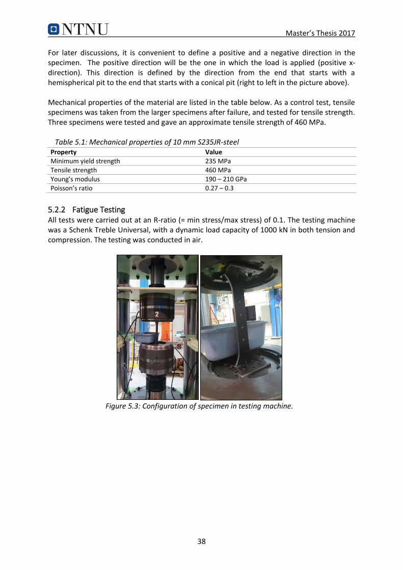
Master’s Thesis 2017
38
For later discussions, it is convenient to define a positive and a negative direction in the specimen. The positive direction will be the one in which the load is applied (positive x-direction). This direction is defined by the direction from the end that starts with a hemispherical pit to the end that starts with a conical pit (right to left in the picture above). Mechanical properties of the material are listed in the table below. As a control test, tensile specimens was taken from the larger specimens after failure, and tested for tensile strength. Three specimens were tested and gave an approximate tensile strength of 460 MPa. Table 5.1: Mechanical properties of 10 mm S235JR-steel
Property Value Minimum yield strength 235 MPa Tensile strength 460 MPa Young’s modulus 190 – 210 GPa Poisson’s ratio 0.27 – 0.3
5.2.2 Fatigue Testing All tests were carried out at an R-ratio (= min stress/max stress) of 0.1. The testing machine was a Schenk Treble Universal, with a dynamic load capacity of 1000 kN in both tension and compression. The testing was conducted in air.
Figure 5.3: Configuration of specimen in testing machine.
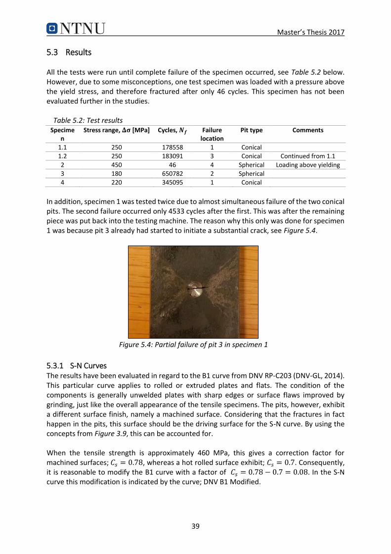
Master’s Thesis 2017
39
5.3 Results All the tests were run until complete failure of the specimen occurred, see Table 5.2 below. However, due to some misconceptions, one test specimen was loaded with a pressure above the yield stress, and therefore fractured after only 46 cycles. This specimen has not been evaluated further in the studies. Table 5.2: Test results
Specimen
Stress range, 𝚫𝛔 [MPa] Cycles, 𝑵𝒇 Failure location
Pit type Comments
1.1 250 178558 1 Conical
1.2 250 183091 3 Conical Continued from 1.1
2 450 46 4 Spherical Loading above yielding
3 180 650782 2 Spherical
4 220 345095 1 Conical
In addition, specimen 1 was tested twice due to almost simultaneous failure of the two conical pits. The second failure occurred only 4533 cycles after the first. This was after the remaining piece was put back into the testing machine. The reason why this only was done for specimen 1 was because pit 3 already had started to initiate a substantial crack, see Figure 5.4.
Figure 5.4: Partial failure of pit 3 in specimen 1
5.3.1 S-N Curves The results have been evaluated in regard to the B1 curve from DNV RP-C203 (DNV-GL, 2014). This particular curve applies to rolled or extruded plates and flats. The condition of the components is generally unwelded plates with sharp edges or surface flaws improved by grinding, just like the overall appearance of the tensile specimens. The pits, however, exhibit a different surface finish, namely a machined surface. Considering that the fractures in fact happen in the pits, this surface should be the driving surface for the S-N curve. By using the concepts from Figure 3.9, this can be accounted for. When the tensile strength is approximately 460 MPa, this gives a correction factor for machined surfaces;𝐶𝑠 = 0.78, whereas a hot rolled surface exhibit; 𝐶𝑠 = 0.7. Consequently, it is reasonable to modify the B1 curve with a factor of 𝐶𝑠 = 0.78 − 0.7 = 0.08. In the S-N curve this modification is indicated by the curve; DNV B1 Modified.

Master’s Thesis 2017
40
Besides, a study conducted by Zhang et al. (2016) argues that the B1 curve historically is based on fatigue tests from specimens with continuous longitudinal butt welds, and therefore exhibit high tensile residual stresses. As a result, the effective R-ratio is found to be 𝑅 = 0.76, which is substantially over the R-ratio used in our tests (𝑅 = 0.1). The study further proposes an alternative design curve for 𝑅 = 0.1, where 𝑚 = 8.3 and 𝐶 = 3.23 ∙ 1026 in reference to Eq. (5.1). Consequently, this introduces an additional reference curve. In order to compare the data, the results have been plotted in a S-N diagram with logarithmic axes. A statistical analysis has been made on the data, resulting in a relevant regression line for comparison. An ordinary linear regression has been used, with the least square method for fitting of a straight line. Since the values are plotted in a log-log plot, the following regression model has been adopted: 𝑁 = 𝐶(Δσ)𝑚 (5.1)
𝑙𝑜𝑔(𝑁) = 𝑙𝑜𝑔(𝐶) + 𝑚 𝑙𝑜𝑔(𝛥𝜎) (5.2)
Eq. (5.1) is similar to the one in Eq. (3.25), together with associated parameters. As the sample points are closely distributed, the estimate of the slope is rather uncertain. Consequently, the analysis was carried out in two ways: one with the slope as a free parameter, and one with 𝑚 equal to the DNV-curves. The results of this statistical analysis can be seen in Table 5.3. Table 5.3: Results of statistical analysis of test data
Regression line Slope parameter, m Standard deviation Goodness of fit C
Free 3.93 0.40 0.985 4.88 x 10¹⁴
B1 4 0.33 0.985 7.24 x 10¹⁴
B1 (R=0.1) 8.3 0.30 - 9.08 x 1024
The statistical analysis is performed through a combination of the software Edna60 and Microsoft Excel. Edna60 is a software entirely devoted to the creation and evaluation of S-N curves. Regression lines were calculated in Excel, and controlled in Edna60. The values in Table 5.3, are taken directly from the latter. The values for standard deviation seems strange. The free slope parameter appears to correspond best with the original B1 curve, yet the B1 curve for 𝑅 = 0.1 produces best values for the standard deviation. However, visual inspection of the lines clearly shows a bad correlation when 𝑚 = 8.3. This is further backed by the software’s failed attempt to produce a value for the goodness of fit at this slope. This might be an indication that the B1 line is the most appropriate reference line. On the other hand, the sample is quite small, and might therefore not represent a sufficiently reliable trend. Therefore, both curves will be preserved. However, additional tests, at a wider range of load levels, should be conducted in future work.

Master’s Thesis 2017
41
The design curve is taken directly from values in DNV RP-C203, while the mean curve is created by the following formula: 𝑙𝑜𝑔(𝐶) = 𝑙𝑜𝑔(𝐶) − 2𝑠𝑙𝑜𝑔𝑁 (5.3)
Where 𝑠𝑙𝑜𝑔𝑁 is standard deviation of 𝑙𝑜𝑔(𝑁). A typical standard deviation of 𝑠𝑙𝑜𝑔𝑁 = 0.200 is
commonly used for the standard S-N curves in DNV-GL (2014) For both S-N curves the test data are below the design curve for plain plate material. This indicates that artificial corrosion pits have a significant effect on the fatigue life. The decrease in fatigue life due to the pits, show to be 37% if compared with the modified B1 mean curve and 46% if compared to the modified B1 (𝑅 = 0.1)mean curve. Defined as an effective correction factor, these values are 𝐶𝑓 = 0.63 and 𝐶𝑓 = 0.54, respectively. This correction
factor is introduced by the author, simply for comparison reasons. It can be derived from the following formula: Δσ𝑚𝑜𝑑 = 𝐶𝑓Δσ0 (5.4)
Where Δσ0 is the fatigue limit at 𝑁 = 107. The formula is similar to what was seen in Eq. (3.24).
Figure 5.5: Test results compared with the DNV B1 curve
10
100
1000
1E+04 1E+05 1E+06 1E+07
Stre
ss r
ange
(M
Pa)
Number of cycles to failure (N)
Test - 1.1Test - 1.2Test - 3Test - 4Test - regression lineDNV B1 DesignDNV B1 MeanDNV B1 Modified

Master’s Thesis 2017
42
Figure 5.6: Test results compared with B1 (R=0.1) curve
10
100
1000
1E+04 1E+05 1E+06 1E+07
Stre
ss r
ange
(M
Pa)
Number of cycles to failure (N)
Test - 1.1Test - 1.2Test - 3Test - 4Test - regression lineDNV B1 Design (R=0.1)DNV B1 Mean (R=0.1)DNV B1 Modified (R=0.1)

Master’s Thesis 2017
43
5.4 Similar Tests DNV-GL have, on contract with Statoil ASA, performed tests on actual mooring chain that have been in active service for approximately 10-12 years (Fredheim et al., 2013). The aim of the tests was to establish the importance of the chain surface condition, such as corrosion and mechanical wear. The tests were performed in a 750 tons’ capacity testing machine, on studless chains of grade R4, with diameter 114 and 126 mm. Statoil have retrieved the chain lengths from the mooring systems of the semi-submersible platform, Njord A, as well as from the FPSO vessel, Åsgard A. The following will focus on the Åsgard chains, as these were to only ones to show severe pitting corrosion.
Figure 5.7: Chain from Åsgard A (left) and testing rig (right). (Fredheim et al. (2013), p. 3 and 6)
The results from the DNV-tests have been plotted in Figure 5.8, on the next page. The regression line is computed by the author in a similar manner as above, using 𝑚 = 3 as a forced slope parameter. The effective correction factor was found to be 𝐶𝑓 = 0.62, indicating
a substantial effect of the pitting corrosion. The S-N curves in Figure 5.8 are provided by Vicinay Cadenas and DNV-GL, and expressed in Table 5.4. The curve is established for new R4 and R5 grade chain tested in seawater conditions. The Njord A chains are produced by Vicinay, while the Åsgard A chains were made by Hamanaka Chain in Japan. However, as Fredheim et al. (2013) were not able to retrieve fatigue curves for Hamanaka Chain, the Vicinay curve is used for comparison purposes. The Åsgard A chains are high strength R4 chain, so the comparison is relevant. Table 5.4: S-N curves for Åsgard A chain
S-N curves
Vicinay – mean curve 𝑁 = 3.6 ∙ 1011(Δσ)3
DNV approved Vicinay curve 𝑁 = 1.41 ∙ 1010(Δσ)3
Regression line 𝑁 = 8.39 ∙ 1010(Δσ)3
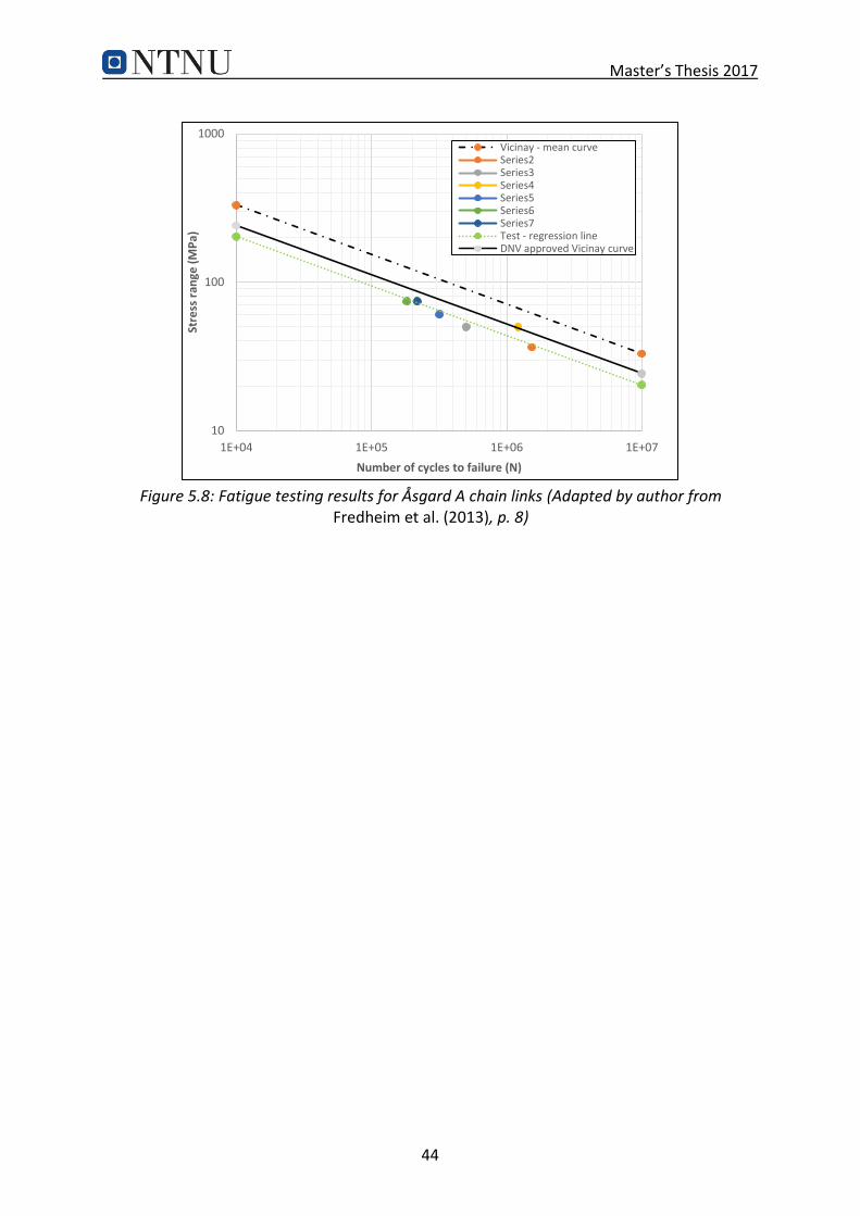
Master’s Thesis 2017
44
Figure 5.8: Fatigue testing results for Åsgard A chain links (Adapted by author from Fredheim et al. (2013), p. 8)
10
100
1000
1E+04 1E+05 1E+06 1E+07
Stre
ss r
ange
(M
Pa)
Number of cycles to failure (N)
Vicinay - mean curveSeries2Series3Series4Series5Series6Series7Test - regression lineDNV approved Vicinay curve

Master’s Thesis 2017
45
6 Finite Element Analysis This study has investigated the effect of stress concentration factors in uniaxial loaded corrosion pits. The investigations have been conducted through a series of 3D stress analyses, performed in the finite element software, ABAQUS/CAE 6.14, henceforth referred to as ABAQUS. The beginning of this chapter will introduce some basic concepts of the finite element method, and review the process of creating a relevant model for this particular case. Finally, actual scans produced with a 3D-scanner, will be introduced for analyses. Finite Element Analysis (FEA), also called the Finite Element Method (FEM), is a method for numerical solution of field problems. Mathematically, a field problem is described by differential equations or by an integral expression. The essence of the method is to idealize a physical problem into a mathematical model, and calculate approximate values of the solutions desired (pressure, stress, temperature, etc.). (George, 1991) In order to solve the mathematical problem, the model is discretized by dividing it into a mesh with elements of finite size. Each element has a certain amount of nodes and degrees of freedom. Elements are connected to other elements in the nodes, eventually creating an entire mesh of elements. The mesh is represented by a system of algebraic equations, that is solved for unknowns at the nodes. Thus, the field quantity over the entire structure is approximated element by element, in a piecewise fashion, hence the element method. (Cook et al., 2002)
6.1 Constructing the Model The purpose of a FEM simulation is to approximate a real life problem. Through reasonable loads and boundary conditions, this can be done rather truthfully. Chapter 5 have already described the actual tests of four tensile specimens. The aim of this section is to explain how these tests, in a best way possible, can be represented in a finite element analysis. The Stress-Based approach will be used to calculate a relevant stress concentration factor for the specimens. As we are only interested in the fatigue life of the component, the calculation of a theoretical stress concentration factor will do. As previously described, this factor is mainly dependent on geometry and loading. Hence, a linear elastic material model will be deployed. The mechanical drawing in Figure 5.1 is based on a CAD-model created in SOLIDWORKS. This model has been imported to ABAQUS for use in the FEM simulations.
6.1.1 Loads and Boundary Conditions The tests are prepared on a classical dog-bone specimen, with the middle section being the part of interest. The end sections are only there as a security – to make sure that fracture occurs in the portion we are interested in. The CAD-model for the dog-bone specimens have been the cornerstone of the finite element model, and has been used in almost all the analyses. This piece has acted as the global model,
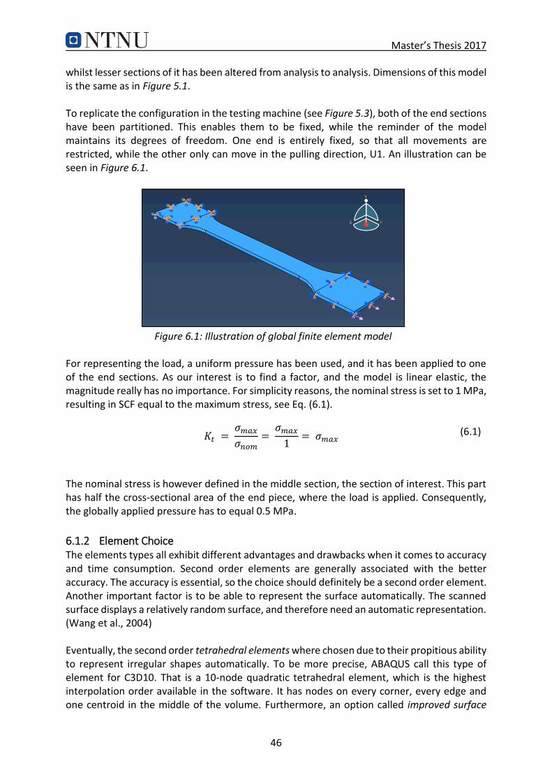
Master’s Thesis 2017
46
whilst lesser sections of it has been altered from analysis to analysis. Dimensions of this model is the same as in Figure 5.1. To replicate the configuration in the testing machine (see Figure 5.3), both of the end sections have been partitioned. This enables them to be fixed, while the reminder of the model maintains its degrees of freedom. One end is entirely fixed, so that all movements are restricted, while the other only can move in the pulling direction, U1. An illustration can be seen in Figure 6.1.
Figure 6.1: Illustration of global finite element model
For representing the load, a uniform pressure has been used, and it has been applied to one of the end sections. As our interest is to find a factor, and the model is linear elastic, the magnitude really has no importance. For simplicity reasons, the nominal stress is set to 1 MPa, resulting in SCF equal to the maximum stress, see Eq. (6.1). 𝐾𝑡 =
𝜎𝑚𝑎𝑥
𝜎𝑛𝑜𝑚=
𝜎𝑚𝑎𝑥
1= 𝜎𝑚𝑎𝑥
(6.1)
The nominal stress is however defined in the middle section, the section of interest. This part has half the cross-sectional area of the end piece, where the load is applied. Consequently, the globally applied pressure has to equal 0.5 MPa.
6.1.2 Element Choice The elements types all exhibit different advantages and drawbacks when it comes to accuracy and time consumption. Second order elements are generally associated with the better accuracy. The accuracy is essential, so the choice should definitely be a second order element. Another important factor is to be able to represent the surface automatically. The scanned surface displays a relatively random surface, and therefore need an automatic representation. (Wang et al., 2004) Eventually, the second order tetrahedral elements where chosen due to their propitious ability to represent irregular shapes automatically. To be more precise, ABAQUS call this type of element for C3D10. That is a 10-node quadratic tetrahedral element, which is the highest interpolation order available in the software. It has nodes on every corner, every edge and one centroid in the middle of the volume. Furthermore, an option called improved surface
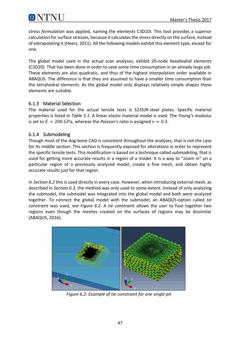
Master’s Thesis 2017
47
stress formulation was applied, naming the elements C3D10I. This tool provides a superior calculation for surface stresses, because it calculates the stress directly on the surface, instead of extrapolating it (Heers, 2011). All the following models exhibit this element type, except for one. The global model used in the actual scan analyses, exhibit 20-node hexahedral elements (C3D20). That has been done in order to save some time consumption in an already large job. These elements are also quadratic, and thus of the highest interpolation order available in ABAQUS. The difference is that they are assumed to have a smaller time consumption than the tetrahedral elements. As the global model only displays relatively simple shapes these elements are suitable.
6.1.3 Material Selection The material used for the actual tensile tests is S235JR-steel plates. Specific material properties is listed in Table 5.1. A linear elastic material model is used. The Young’s modulus is set to 𝐸 = 200𝐺𝑃𝑎, whereas the Poisson’s ratio is assigned 𝜈 = 0.3.
6.1.4 Submodeling Though most of the dog-bone CAD is consistent throughout the analyses, that is not the case for its middle section. This section is frequently exposed for alterations in order to represent the specific tensile tests. This modification is based on a technique called submodeling, that is used for getting more accurate results in a region of a model. It is a way to “zoom in” on a particular region of a previously analyzed model, create a fine mesh, and obtain highly accurate results just for that region. In Section 6.2 this is used directly in every case. However, when introducing external mesh, as described in Section 6.3, the method was only used to some extent. Instead of only analyzing the submodel, the submodel was integrated into the global model and both were analyzed together. To connect the global model with the submodel, an ABAQUS-option called tie constraint was used, see Figure 6.2. A tie constraint allows the user to fuse together two regions even though the meshes created on the surfaces of regions may be dissimilar (ABAQUS, 2016).
Figure 6.2: Example of tie constraint for one single pit

Master’s Thesis 2017
48
6.2 Validation of the Model Prior to testing the actual scans, a study of comparable ideal geometries was conducted. The idea was to start with something simple and gradually work towards the desired scenario. When working with ideal shapes, it was possible to find analytical solutions to the problems, and eventually use these to confirm the model. Certainly arriving at similar solutions as acknowledged literatures would be a good indication of the methods capabilities.
6.2.1 Previous Studies Several shapes and features were investigated, but the most promising was by far the hemispherical pit in a semi-infinite body. Consequently, this was chosen as the first step of the validation study. A wide range of studies was discovered on this particular scenario. Some of the studies involved numerical solutions similar to this case (Eksi et al. (2009), Turnbull et al. (2010), Kolios et al. (2014)), while others were associated with analytical explanations (Fujita et al. (1982), Eubanks (1953)). Eubanks looked into the situation of a hemispherical pit exposed to biaxial tension, whereas Fujita covered the uniaxial case. As this project involves uniaxial tension, that will be the focus. Eubanks had earlier concluded that the maximum stress appeared in the bottom of the pit when the loading was biaxial, so it was with some astonishment Fujita found the uniaxial load to produce two maximum locations. The locations were found perpendicular to the loading direction, a little distance up the cavity wall. Regarding Figure 6.3, the two points can be established where 𝑅 = 1, 𝜑 = 65°, 𝜃 = 90° and 𝜃 = 270°. The SCFs were found to equal 𝐾𝑡 = 2.062 in the uniaxial case, and 𝐾𝑡 = 2.181 in the biaxial case. Both studies were performed in a semi-infinite body, with an anticipated Poisson’s ratio of 𝜈 = 0.3. The nominal stress was referred to in the gross cross-sectional area, whereas maximum stress was given as maximum principal stress.
Figure 6.3: Coordinate system (Fujita et al. (1982), p.2)

Master’s Thesis 2017
49
The study conducted by Eksi et al. (2009), uses numerical calculations in ANSYS to investigate a series of three-dimensional semi-elliptical pitted models. In the hemispherical pit, the critical area is found to lie between base and mouth of the pit, as a band perpendicular to the loading direction. The maximum stress occurs slightly below the mouth of the pit, and has a value a little above what was seen in Fujitas study (𝐾𝑡 = 2.1). Below this point the stress varies less than 1% throughout the described band. Furthermore, the study has identified the pit aspect ratio (pit depth 𝑎/pit diameter 𝑑) as the main parameter effecting the stress concentration factor. Similar findings are derived in the studies of Turnbull et al. (2010) and Kolios et al. (2014).
6.2.2 Recreation of Analytical Results The first on the agenda, was to recreate the problem in Fujita et al. (1982). Fujita and his team used a semi-infinite body in their calculations. The account for this, the model was made rather large compared to the cavity. The dimensions were as follows; Length 𝐿 = 200𝑚𝑚, width 𝐻 = 200𝑚𝑚 and thickness ℎ = 100𝑚𝑚. An illustration of the model can be seen in Figure 6.4. In the center of the top plane lies a hemispherical pit with radius 𝑟 = 4𝑚𝑚. Due to symmetry reasons, only ¼ of the model needed to be analyzed. A uniform pressure was used for the load, with a magnitude of 1 MPa. The boundary conditions were set to x-symmetry (U1 = UR2 = UR3 = 0) in the x-direction and z-symmetry (U3 = UR1 = UR2 = 0) in the z-direction. (Aryarad and Heshmati, 2015)
Figure 6.4: Large body with small hemispherical pit in one of the free surfaces. The left model illustrates the entire body, whereas the right display one
quarter.
Submodeling was used in this particular analysis because the requirement of a very fine mesh was needed in order to get the maximum stress to converge. Figure 6.5, on the next page, shows an illustration of the convergence study. When the elements increase, so does the maximum stress in the first two or three analyses. However, after some time the stress will converge to the same value. The maximum von Mises settle at around 𝜎𝑒𝑞 = 2.02𝑀𝑃𝑎, which
gives a stress concentration equal to 98% of the analytical 𝐾𝑡, and thus seems like a reasonable result. Furthermore, if we consider the maximum principal stress, as can be seen in Figure 6.6, this value converge at 𝐾𝑡 = 2.068. That is only 0.29% off from the analytical value, and is thus a very accurate result.
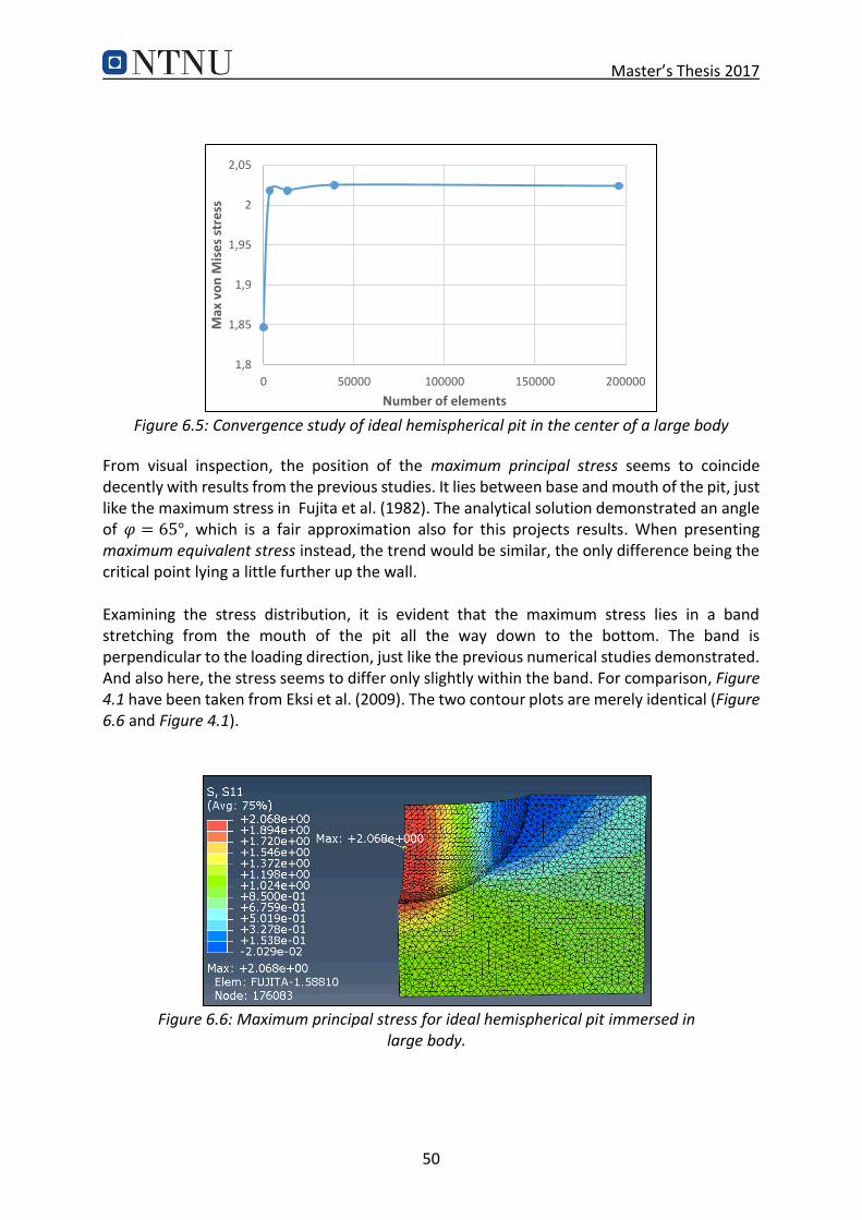
Master’s Thesis 2017
50
Figure 6.5: Convergence study of ideal hemispherical pit in the center of a large body
From visual inspection, the position of the maximum principal stress seems to coincide decently with results from the previous studies. It lies between base and mouth of the pit, just like the maximum stress in Fujita et al. (1982). The analytical solution demonstrated an angle of 𝜑 = 65°, which is a fair approximation also for this projects results. When presenting maximum equivalent stress instead, the trend would be similar, the only difference being the critical point lying a little further up the wall. Examining the stress distribution, it is evident that the maximum stress lies in a band stretching from the mouth of the pit all the way down to the bottom. The band is perpendicular to the loading direction, just like the previous numerical studies demonstrated. And also here, the stress seems to differ only slightly within the band. For comparison, Figure 4.1 have been taken from Eksi et al. (2009). The two contour plots are merely identical (Figure 6.6 and Figure 4.1).
Figure 6.6: Maximum principal stress for ideal hemispherical pit immersed in large body.
1,8
1,85
1,9
1,95
2
2,05
0 50000 100000 150000 200000
Max
vo
n M
ise
s st
ress
Number of elements

Master’s Thesis 2017
51
Figure 6.7: Maximum principal stress in hemispherical pit (Eksi et al. (2009), p. 2469)
Now that it is confirmed that FEA is able to arrive at similar solutions as the analytical values, the validation of a more realistic case can be assessed. Therefore, the global model from Section 6.1 will be introduced. This specimen is both slimmer and thinner than the situation of the large body, and is thus expected to demonstrate slightly different 𝐾𝑡-values. The pit will be positioned in the center of the global model. The loads and boundary conditions are as described in Section 6.1. Submodelling is used on a lesser section with the pit. Also for this analysis, it is evident that the results converge relatively fast, see Figure 6.8. As expected there is a slight jump in the 𝐾𝑡-values (𝐾𝑡 = 2.197, 𝐾𝑡
′ = 2.167). This jump is a result of decreased width and thickness. This time the maximum von Mises stress is illustrated, and can be seen in Figure 6.9. As described earlier, this value is located a little higher up the cavity wall compared to the position of the principal stress.
Figure 6.8: Convergence study of ideal hemispherical pit in tensile specimen
2,165
2,166
2,167
2,168
2,169
2,17
2,171
2,172
2,173
0 100000 200000 300000 400000 500000
Max
vo
n M
Ise
s st
ress
Number of elements

Master’s Thesis 2017
52
Figure 6.9: Maximum equivalent stress for ideal hemispherical pit immersed
in a tensile specimen
Thus far, only simple geometries have been investigated, especially compared to the conical pit. To get a more realistic scenario, the complexity of the model needs to increase. Hence, the following will make an analysis of the actual CAD-model. Figure 6.10 shows a cross section of the CAD-pits. As can be seen from Figure 6.10 a), some of the features demonstrate sharp edges, like the one in the bottom of the conical pit. Edges like this may eventually introduce singularities, which can be detrimental for the final stress convergence. As a result, the pits are smoothed as illustrated in Figure 6.10 b). Not only will this solve the problem with the singularities, it will make the features look more like the actual case (see Figure 6.10 c)). The fillet in the conical pit has a radius of 𝑟 = 1.5𝑚𝑚, whereas the one introduced in the hemispherical has a radius equal 𝑟 = 0.5𝑚𝑚. Stress singularities appear in sharp corners, eventually making the stress in these areas infinitely large. The stress will keep growing no matter how fine the mesh is made. Of course, such infinite stresses do not exist in real life, it is merely a theoretical phenomenon. But this theoretical phenomenon will be pertinent in a FEA as long as measures are not taken. Even when a perfect CAD geometry is possible, it is common practice to defeature the geometry to remove small details that are not important within the scope of the analysis. (Sönnerlind, 2015, Frei, 2013)
a) b) c)
Figure 6.10: a) cross section of CAD-pits, b) cross section of modified CAD-pits and c) cross section of scanned pits

Master’s Thesis 2017
53
The modified CAD-pits has been modeled as described in Section 6.1. Convergence studies result in 𝐾𝑡 = 2.233 and 𝐾𝑡
′ = 2.188 for the hemispherical pit, and 𝐾𝑡 = 2.571 and 𝐾𝑡′ =
2.444 for the conical pit. The stress distributions is illustrated in Figure 4.1 and Figure 6.12.
Figure 6.11: Maximum von Mises in hemispherical CAD-pit
Figure 6.12: Maximum von Mises in conical CAD-pit Finally, expected values for both the conical and hemispherical pit have been derived, and the study can move on to introduce the actual scans of the pits. It is interesting to note the difference of roughly 10% between the two pit categories. Before we move on, a table summarizing the different convergence studies, is presented on the next page. Relevant information will be extracted from this table in later sections. The most adaptable parameter is probably the element size, which eventually will be adopted for the scanned surfaces. From the table, it is reasonable to the assume that convergence happens at an element size equal to 0.4 mm. The element size is typically defined as for the diameter in Figure 6.13, represented by ℎ𝐾.

Master’s Thesis 2017
54
Figure 6.13: Diameter and sphericity for a triangular element (left) and quadrilateral element (right). (Quarteroni (2014), p. 144)
Table 6.1: Summary of convergence results
Case Elements Element size [mm] Max principal [MPa] Max von Mises [MPa]
Ideal hemispherical (large body)
108 5 1,901 1,847 3379 1 2,06 2,018 13181 0,6 2,074 2,018 39215 0,4 2,071 2,025 196275 0,2 2,068 2,024
Ideal hemispherical (tensile specimen)
5988 1 2,224 2,172 23181 0,6 2,2 2,166 69903 0,4 2,197 2,166 424677 0,2 2,197 2,166
Hemispherical CAD 3634 1 2,22 2,175 12344 0,6 2,227 2,179 38984 0,4 2,231 2,198 247841 0,2 2,233 2,188
Conical CAD 4184 1 2,578 2,394 15088 0,6 2,566 2,428 45293 0,4 2,57 2,444 296520 0,2 2,571 2,444

Master’s Thesis 2017
55
6.2.3 Convergence of Global Model
Figure 6.14: Final assembly of tensile stress specimens
Figure 6.14 shows the final assembly of the scanned pits embed into the global model. Thus far, the focus has been on getting reliable results from the submodel. However, those numbers mean little if the global model presents unrealistic results. The above calculations have been based on the assumption that 𝜎𝑛𝑜𝑚 = 1𝑀𝑃𝑎, in the middle section of the global model. That can be confirmed by looking at a simple convergence study of the global model. The figure below illustrates what happens in the global model when the elements are refined. The contour is set to show values from 1 MPa and upwards, with blue color indicating 1MPa. Just from visual inspection, it is clear that the section with the scans, always will experience the same stress.
Figure 6.15: Simple convergence of global model
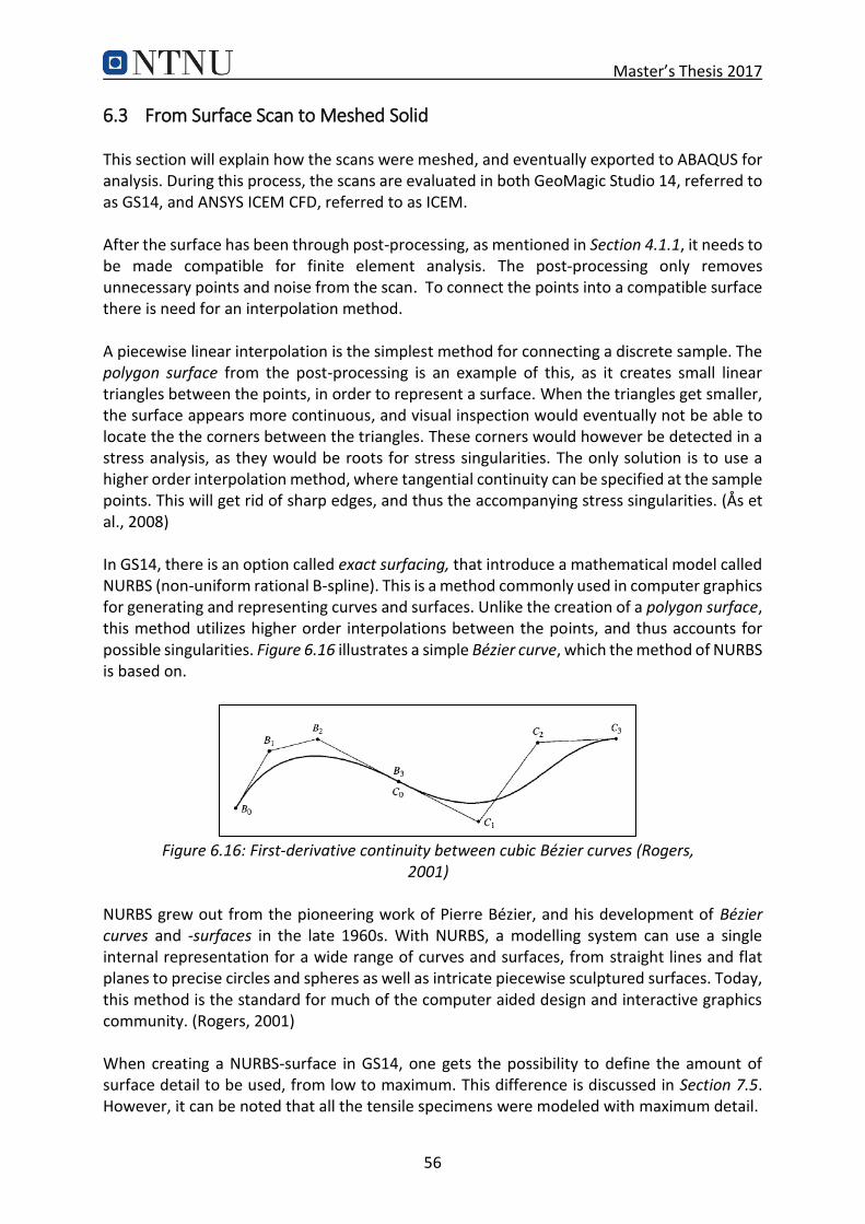
Master’s Thesis 2017
56
6.3 From Surface Scan to Meshed Solid This section will explain how the scans were meshed, and eventually exported to ABAQUS for analysis. During this process, the scans are evaluated in both GeoMagic Studio 14, referred to as GS14, and ANSYS ICEM CFD, referred to as ICEM. After the surface has been through post-processing, as mentioned in Section 4.1.1, it needs to be made compatible for finite element analysis. The post-processing only removes unnecessary points and noise from the scan. To connect the points into a compatible surface there is need for an interpolation method. A piecewise linear interpolation is the simplest method for connecting a discrete sample. The polygon surface from the post-processing is an example of this, as it creates small linear triangles between the points, in order to represent a surface. When the triangles get smaller, the surface appears more continuous, and visual inspection would eventually not be able to locate the the corners between the triangles. These corners would however be detected in a stress analysis, as they would be roots for stress singularities. The only solution is to use a higher order interpolation method, where tangential continuity can be specified at the sample points. This will get rid of sharp edges, and thus the accompanying stress singularities. (Ås et al., 2008) In GS14, there is an option called exact surfacing, that introduce a mathematical model called NURBS (non-uniform rational B-spline). This is a method commonly used in computer graphics for generating and representing curves and surfaces. Unlike the creation of a polygon surface, this method utilizes higher order interpolations between the points, and thus accounts for possible singularities. Figure 6.16 illustrates a simple Bézier curve, which the method of NURBS is based on.
Figure 6.16: First-derivative continuity between cubic Bézier curves (Rogers, 2001)
NURBS grew out from the pioneering work of Pierre Bézier, and his development of Bézier curves and -surfaces in the late 1960s. With NURBS, a modelling system can use a single internal representation for a wide range of curves and surfaces, from straight lines and flat planes to precise circles and spheres as well as intricate piecewise sculptured surfaces. Today, this method is the standard for much of the computer aided design and interactive graphics community. (Rogers, 2001) When creating a NURBS-surface in GS14, one gets the possibility to define the amount of surface detail to be used, from low to maximum. This difference is discussed in Section 7.5. However, it can be noted that all the tensile specimens were modeled with maximum detail.

Master’s Thesis 2017
57
6.3.1 Modelling in ICEM Much of the modeling in ICEM have been adapted from Hoel’s work (Hoel, 2016). There are however some exceptions – procedures that the author has found it necessary to adapt. This section will introduce some key procedures, and discuss their relevance. For a more detailed review of the basic procedures the reader is referred to Hoel (2016) or the step-by-step guide added in Appendix A. After introducing NURBS to the scanned surfaces, they are finally ready for meshing, and can be exported to ICEM. The files are exported in iges-format, and opened under legacy geometry in ICEM. Before the surfaces can be used in a FEA, they need to have an accompanying body, and this body needs to be meshed. ICEM provides advanced geometry acquisition, mesh generation, and mesh diagnostic to provide integrated mesh generation for today’s sophisticated analyses ((ANSYS ICEM CFD, 2016a)). Thus, it is ideal for converting the surfaces into solid meshed components. The modelling functions in ICEM enables the user to define walls around a surface geometry. This was used to create a closed and hollow box, where one of the six sides was represented by the scanned surface. This box was later meshed with volume elements. As the boxes need to fit perfectly in the global model, the dimensioning requires careful consideration. The top surface is extended, in order to give it exact dimensions, and subsequently extruded 10 mm, to give it the same thickness as the dog-bone specimens. The dimensions of the top surface varied with the respective model. The figure below shows an example where the single hemispherical pit, used for convergence of the scans, is illustrated. Whenever an entire specimen was modelled, the top surface had a dimension equal 165x15 mm.
Figure 6.17: Meshed ICEM-model of single hemispherical pit
After modeling the box, and before introducing the mesh, the model should always undergo the build topology tool. This tool automatically extracts curves and points from surface edges and corners, forcing the mesh nodes to lie along the respective features of the geometry. The extracted features depend on the proximity of the surface edges to each other. Figure 6.18 shows an example where the first picture illustrates the curves and points representing the geometry. The second picture shows the result when the features are preserved in the geometry, while the last illustrates what will happen if the curves and points are deleted from the geometry.

Master’s Thesis 2017
58
Figure 6.18: Effect of build topology (ANSYS ICEM CFD, 2016b)
The model is now ready for meshing, and an appropriate meshing procedure should be selected. The final goal of the mesh is to get the results to converge. If the results do not converge, they are not reliable. Previous examples have highlighted mesh refinement as an effective method of achieving convergence. This will be adapted to the scanned specimens. However, as these models are meshed in ICEM, and not ABAQUS, alternate refinement solutions must be investigated. Hoel (2016) suggests the use of The Octree (Robust) method for meshing. This method generates a volume mesh using a top-down approach, which will make the volume mesh conformal to the geometry and generate a patch-independent surface mesh at all the boundaries and internal walls. The method ensures refinement of the mesh where necessary, but maintains larger elements where possible, enabling faster computation. It is regarded as a good alternative, and will thus be adapted in this work. However, this method alone is not sufficient for refining specific areas more than others. It is further suggested by Hoel (2016) to use a tool called proximity based refinement. This is an accompanying tool to the The Octree (Robust) method, which is supposed to allow for a fine mesh in areas with complex geometry, and coarser mesh in areas with simple geometry. Although this sounds good, it will produce a huge amount of elements in areas of no interest, eventually making the files very large, and that is not feasible. The tool could be used, but it

Master’s Thesis 2017
59
should not be the mere solution for refining the mesh. Alternatively, it could be used when the sufficient element size is found. Alternate options for refining the mesh are the density tool and the part mesh tool. The density tool creates a box where all features covered by the box can be denoted with an alternative element size to that of the global model. The part mesh, on the other hand, is a straight forward way of assigning different mesh characteristics to different parts. Separate parts can be created for each pit, selecting the relevant NURBS-patches in these areas. The different parts are eventually assigned an element size, of the users’ choice. The part mesh was regarded as the best solution in this project. During meshing, an option called smoothing was enabled. This is an iterative process that modifies the quality of the mesh. The quality can be defined in numerous ways, but the most common definition is based on the element aspect ratio. This value is calculated differently in all types of elements, however, the main idea is to maintain a perfectly regular element as far as it is possible. The values are scaled so that 1 represents a perfectly regular element, while 0 indicates that an element has zero volume. The aspect ratio for a tetra element is given by the following formula:
𝐴𝑠𝑝𝑒𝑐𝑡𝑅𝑎𝑡𝑖𝑜 = (𝑉 𝑟3⁄ )
𝑎𝑐𝑡𝑢𝑎𝑙
(𝑉 𝑟3⁄ )𝑖𝑑𝑒𝑎𝑙
(6.2)
Where 𝑉 is the volume of the element and 𝑟 is the radius of the circumscribed sphere. Actual represent the current element, while ideal is a perfectly regular element. The smoothing was set to not give values below 0.4. After meshing, usually only a few elements were found to display this value, whereas the majority displayed an aspect ratio equal to 1. Eventually, when the model is properly meshed, it can be exported to an appropriate finite element software. As this project have used ABAQUS, the files were converted to ABAQUS input files, of .inp-format. The figure below shows a finished ICEM-mesh embed in the global ABAQUS-model. ICEM did not have the ability to produce C3D10 elements, so the elements had to be converted from C3D4 once imported. This conversion enhances the nodes of the elements, adding one to every edge and one in the centroid, while the shape of the elements stays the same.
Figure 6.19: Scanned tensile test, meshed in ICEM and exported to ABAQUS

Master’s Thesis 2017
60
6.4 The Scanned Specimens Finally, the actual scans can be submitted for analysis. The meshed scans are exported to ABAQUS, and combined with the global model, as described in Section 6.1. As the aim is to get converged results, several versions of each specimen is imported, with minimum element size fluctuating from 0.4 mm to 0.05 mm. The highest value was chosen from where the ideal geometries were seen to converge. Due to the irregularities, the scanned specimens are expected to require even more refining. To save time and disk space, only one conical pit and one hemispherical pit was tested for convergence. Afterwards, the associated parameters were used for all the tensile tests. Final simulation results for the four tensile specimens are introduced and discussed in Chapter 7. Two plots describing the convergence is illustrated below. The first shows convergence in regard to the number of elements, and the other to the element size. In both pit categories the stress converges at roughly 0.1 mm. This gives a concentration factor of 𝐾𝑡
′ = 2,61 for the conical pit and 𝐾𝑡
′ = 2,20 for the hemispherical one.
Figure 6.20: Convergence of scanned pits, regarding the number of elements
Figure 6.21: Convergence of scanned pits, regarding the element size
2,1
2,2
2,3
2,4
2,5
2,6
2,7
0 100000 200000 300000 400000 500000
Max
vo
n M
ise
s st
ress
[M
Pa]
Number of elements
Hemispherical Conical
2,1
2,2
2,3
2,4
2,5
2,6
2,7
00,10,20,30,40,5
Max
vo
n M
ise
s st
ress
[M
Pa]
Element size [mm]
Hemispherical Conical

Master’s Thesis 2017
61
6.5 An Actual Corrosion Pit Thus far, all the analyses have dealt with either ideal geometries or scanned artificial pits. Although the method has been confirmed for these simplified scenarios, a test of the real case still remains. This section will address this last obstacle, and prove the methods capability for real corrosion pits. Hoel (2016) tried to analyze one single corrosion pit in his thesis, but failed to give credible results, as the values never converged. There could be several reasons for this, but the most detrimental is seemingly the lack of practical surfaces. Recalling the stress singularities discussed in Section 6.3, it is evident that a surface created by linear interpolations will have troubles converging. To cope for this, the current thesis has utilized higher order interpolations, effectively removing small singularities. The mathematical model called NURBS, is to thank for this. This procedure alone, is expected to result in converged results. Moreover, a different method for mesh refinement has been introduced. Instead of the rather overwhelming proximity based refinement, a very direct method has been deployed for specific convergence of relevant areas (see Section 6.3.1). Together, these procedures were expected to cause convergence.
Figure 6.22: Stress distribution in corrosion pit subjected to uniaxial loading. The element size is 0.4 mm.
For consistency in the project, the exact same pit as utilized in Hoel (2016), have been analyzed in this work, see Figure 6.22. However, for simplicity, the pit was added to a tensile specimen similar to the ones used in the laboratory tests. Prior to analysis, the surface of the pit was converted to a NURBS-surface and meshed as described in Section 6.3. Subsequently, two simulations were run – one converged and one did not. The first attempt employed maximum surface detail when converting to NURBS-surface, because this was the practice from earlier specimens. It was a desire to use surfaces that was as identical as possible to the real case. However, convergence was not achieved, and thus another attempt with a minimum amount of detail was endeavored. This time the analysis succeeded, meaning that the maximum stress finally converged. A table summarizing the analyses is added in Chapter 7 for further discussion (Table 7.9).

Master’s Thesis 2017
62
7 Results and Discussion The results from the finite element analysis will be introduced and compared up against the outcomes of the laboratory test. Both the crack fronts and the prediction of lifetime will be discussed. Finally, the outcomes for an actual corrosion pit will be considered.
7.1 Critical Pits Analyses was run on all four tensile tests. The first round was meant to locate the critical areas for the subsequent analyses, and was thus run with an element size of 0.4 mm. This size was chosen from the convergence of the ideal shapes (Section 6.2). After locating the critical areas in the first round of analyses, all the specimens were refined according to the convergence study of the scanned pits (Section 6.4). That resulted in a final element size of 0.1 mm in the critical areas. The results are displayed in the table below, and graphics of the most critical pits can be found in Figure 7.1. All specimens exhibit the most critical areas in conical pits. Table 7.1: Maximum stress in tensile specimens
Specimen Element size [mm] Max von Mises [MPa] Pits with stress close to global maximum
1 0.1 2,626 1 and 3
2 0.1 2,645 1 and 3
3 0.1 2,536 All
4 0.1 2,597 1 and 3
a) b)
c) d)
Figure 7.1: The pits with highest SCF in each specimen; a) Pit 1 in tensile test 1, b) pit 1 in tensile test 2, c) pit 1 in tensile test 3 and d) pit 3 tensile test 4

Master’s Thesis 2017
63
7.2 Failure Locations From the results in Table 7.1, it is clear that the conical pits in general experience a higher stress than the hemispherical ones. That correlates well with the results of the ideal shapes. However, it does not correspond entirely with actual tests. The tensile specimens tested in the laboratory experienced failures in both conical and hemispherical pits. In total, only 2/5 failures occurred where it was predicted. This section discusses the failures and attempts to provide reasonable solutions for their behavior(s). The following table illustrates where failure was predicted and where it actually happened, as well as the associated SCF from the simulations. Table 7.2: Failure location – predicted/reality
Failure Predicted pit Actual pit
Number 𝐾𝑡′ Number 𝐾𝑡
′
1.1 1 2.626 1 2.626
1.2 3 2.549 3 2.549
2 1 2.645 4 2.217
3 1 2.536 2 2.396 4 3 2.597 1 2.549
All the analyses generated maximum stress in the conical pits, 1 and 3. It is therefore reasonable to expect failure in these locations. The difference between these pits is often seen to be in the range of 1%, essentially suggesting that failure could occur in either. Consequently, the failure of pit 3 in specimen 4, was somewhat expected. It is more surprising that two failures struck in hemispherical pits. Recalling the ideal shapes, the maximum stress was expected to differ by almost 10% between the two pit categories, with hemispherical displaying the lowest value. This is however not always the case when evaluating the scans. The maximum value between pit 1 and 2 in specimen 3 only deviates with 5.5%. Failure 2 occurs during overloading, and is thus not representative for fatigue failure. One explanation for this behavior, could be the introduction of irregularities from machining. Some of the pits revealed significant defects from the machining process, that may have influenced the stress distribution. The small peak in the bottom of a hemispherical pit in Figure 7.2 is an example of that.
Figure 7.2: Example of machining defects

Master’s Thesis 2017
64
The machining also shows poor consistency in fulfilling the dimensional requirements of the pits. This is another possible factor influencing the stress distribution. Eksi et al. (2009), concluded that stress concentrations of elliptical pits were highly dependent on pit aspect ratios – higher ratios gave higher stress concentrations. By applying the methods in section 4.2.1, the geometry of the pits have been determined, and aspect ratios are listed in Table 7.3. The effects of pit aspect ratios are however not that clear in this study. It may be there, but other factors seem to be superior, like the machining defects. Nevertheless, it could be argued that the difference in aspect ratio between conical and hemispherical pits, seem to be minimal in specimen three, making the stress distribution of each pit more alike. Table 7.3: Aspect ratios of scanned pits
Specimen Aspect Ratio (depth/diameter)
1 2 3 4
1 0.37 0.39 0.37 0.4
2 0.44 0.47 0.45 0.48
3 0.40 0.42 0.42 0.44
4 0.44 0.47 0.44 0.46
Finally, the concept of fatigue stress concentration factor should be discussed. This factor is described in Section 3.5.2, but to summarize; it is an empirical induced factor that can be introduced to give more reasonable results when the local stress exceeds the yield stress. Consequently, if local yielding occurs in the pits, this may eventually alter the effective stress concentration factors, possibly leading to similar results for conical and hemispherical pits. This is highly plausible explanation of the prediction error. The local stress is calculated by multiplying the relevant SCF with the nominal stress. This can be done through any of the three equations; Eq.(3.3), (3.19) or (3.20). Eq. (3.3) is the overall case, while Eq. (3.19) is used for the theoretical stress concentration factor and Eq. (3.20) is used for the fatigue stress concentration factor. Eq. (3.20) is only needed if the local stress exceeds yielding, but in the scenario where that happens, this equation gives the most reasonable results. It is therefore of interest to calculate the maximum stress in the critical pits, to see if yielding occurs. Hence, this is done in Table 7.4, by the use of Eq. (3.19). Table 7.4: Calculation of maximum local stress in failed pits
Failure Stress range, 𝚫𝛔 [MPa] 𝑲𝒕′ Maximum stress, 𝚫𝝈𝒎𝒂𝒙 [MPa]
1.1 250 2.626 657
1.2 250 2.549 637
2 450 2.217 998
3 180 2.396 431
4 220 2.549 561
Recalling that the used material exhibits a minimum yield strength of 235 MPa, it is evident that local yielding will occur in the pits. Consequently, the fatigue stress concentration factor has to be used. This factor is dependent on the theoretical SCF and the notch sensitivity. The notch sensitivity can be estimated from charts like the one in Figure 3.8, when the radius of the pit and the tensile strength is known.
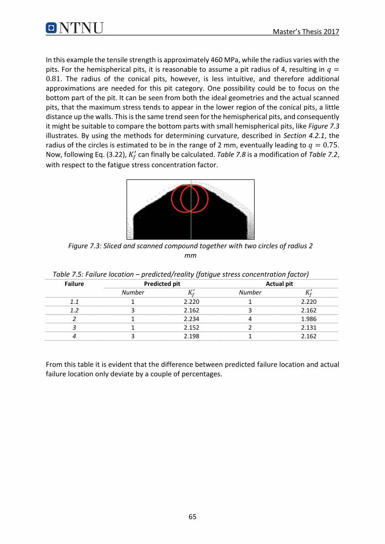
Master’s Thesis 2017
65
In this example the tensile strength is approximately 460 MPa, while the radius varies with the pits. For the hemispherical pits, it is reasonable to assume a pit radius of 4, resulting in 𝑞 =0.81. The radius of the conical pits, however, is less intuitive, and therefore additional approximations are needed for this pit category. One possibility could be to focus on the bottom part of the pit. It can be seen from both the ideal geometries and the actual scanned pits, that the maximum stress tends to appear in the lower region of the conical pits, a little distance up the walls. This is the same trend seen for the hemispherical pits, and consequently it might be suitable to compare the bottom parts with small hemispherical pits, like Figure 7.3 illustrates. By using the methods for determining curvature, described in Section 4.2.1, the radius of the circles is estimated to be in the range of 2 mm, eventually leading to 𝑞 = 0.75. Now, following Eq. (3.22), 𝐾𝑓
′ can finally be calculated. Table 7.8 is a modification of Table 7.2,
with respect to the fatigue stress concentration factor.
Figure 7.3: Sliced and scanned compound together with two circles of radius 2 mm
Table 7.5: Failure location – predicted/reality (fatigue stress concentration factor)
Failure Predicted pit Actual pit
Number 𝐾𝑓′ Number 𝐾𝑓
′
1.1 1 2.220 1 2.220
1.2 3 2.162 3 2.162
2 1 2.234 4 1.986
3 1 2.152 2 2.131
4 3 2.198 1 2.162
From this table it is evident that the difference between predicted failure location and actual failure location only deviate by a couple of percentages.

Master’s Thesis 2017
66
7.3 Crack Surfaces More or less all of the simulations did predict reasonable stress distributions for the actual failure pits. In Figure 7.4 to Figure 7.8, all the failure locations are illustrated with the actual crack surface and the corresponding stress distribution in ABAQUS. The rightmost picture is added to give a more focused distribution of the maximum stress. The pictures are seen in the negative direction, as defined in Section 5.2.1. The area where crack initiation is expected to have started, are marked in all the pictures. The red arrow indicates a suggested crack initiation spot.
Figure 7.4: Failure 1.1 compared to FEA. Failure occurred in pit number 1.
Figure 7.5: Failure 1.2 compared to FEA. Failure occurred in pit number 3.
Figure 7.6: Failure 2 compared to FEA. Failure occurred in pit number 4.

Master’s Thesis 2017
67
Figure 7.7: Failure 3 compared to FEA. Failure occurred in pit number 2.
Figure 7.8: Failure 4 compared to FEA. Failure occurred in pit number 1.
A previous study, conducted by Hove (2016), suggested that hemispherical pits should initiate in the side of the pits. The hypothesis supporting this proposition said that the crack would grow until it reached the same depth as the pit, and then it would start to grow sideways eventually encompassing the pit with an elliptical crack surface. That is exactly what can be seen for the one hemispherical pit that failed due to a fatigue crack, see Figure 7.7. Failure 2, which is illustrated in Figure 7.6, does not have a crack front. That is because this failure occurred during overloading, when the entire model was in the plastic area.
Figure 7.9: Red zone is the initial growth regime, blue is the transition regime and yellow is the stable growth regime (Hove (2016), p. 35)

Master’s Thesis 2017
68
The failures that occurred in the conical pits, all initiated at the bottom side of the pit. This section of the pit can almost be viewed as two small hemispherical pits, see Figure 7.3. If that is considered the case, the hypothesis from Hove (2016) could be applied also for these scenarios. Even here, a small displacement of the crack front can be seen towards the side where the maximum stress occurs. This is especially visible in Figure 7.8, where the crack surface is tilted to the left, when seen in the negative direction. The crack surface seen for the tensile specimens are classical beach marks, as described in Section 3.1. The reason why most of the failures exhibit just one beach mark, is because the cyclic loading is kept constant until failure. The only location that undoubtedly display more than one, is failure 1.2 (Figure 7.5), which has two. This is because specimen 1 first was loaded until failure 1.1, before it was loaded again to produce failure 1.2. The small circle is from the first round. If the specimens are examined closely, whit a microscope, the presence of striations are most likely to be present. However, such examinations are beyond the scope of this thesis.

Master’s Thesis 2017
69
7.4 Predicting Fatigue Life on the Basis of FEM Simulations Finally, it has come to the prediction of final fatigue life of the specimens. Section 3.7 introduced the ultimate idea of the method, this section will resume to perform the calculations. The first concept to account for, is the stress concentration factors. The stress concentration factor is the key parameter for the FEM simulation, and is thus the driving constraint for this entire method. Care must be taken when deciding on the most appropriate SCF, as it may change according to the actual applied loads, like discussed in Section 7.2. As the factor is computed in a linear elastic material model, it does not account for local plastic deformation, it is an ideal theoretical factor. Consequently, if the location of the SCF exceeds yield, 𝐾𝑡
′ no longer is valid. Instead, the solution becomes to introduce the fatigue stress concentration factor, 𝐾𝑓
′. This factor will thus be preferred for estimating the final fatigue life.
As it has been stressed earlier, the S-N curves often need minor adjustments in order to fully represent an actual case. Several correction factors, as described through Sections 3.3 - 3.6, are used in order to make the curves more realistic. The B1 curve has already been recognized as the most appropriate curve for the tensile specimens, and adjusted thereafter. Section 5.3.1 introduced an additional curve for 𝑅 = 0.1 and raised both of them to account for the machined pit surface. These two curves will be used together with the SCF to predict a final lifetime of each specimen. The following formulas, presented again from Eq. (3.3), (3.24) and (3.25), are used to calculate the final fatigue life: 𝜎𝑙𝑜𝑐𝑎𝑙 = 𝑆𝐶𝐹𝜎𝑛𝑜𝑚𝑖𝑛𝑎𝑙 (7.1)
Δσ𝑚𝑜𝑑 = 𝐶𝑠Δσ0 (7.2)
𝑁 = 𝐶(Δσ)𝑚 (7.3)
The results are illustrated in Figure 7.10 and Figure 7.11, and summarized in Table 7.6 and Table 7.7. Table 7.6: Cycles to failure
Failure Cycles to failure, N
B1 Modified B1 Laboratory tests
1.1 47 197 25 680 178 558
1.2 52 446 31 961 183 091
3 171 185 507 066 650 782
4 89 050 80 517 345 095
Table 7.7: Correction factors for FEA results
FEA – regression line Effective correction factor, 𝑪𝒇 Factor of test regression line, 𝑪𝒇𝟐
B1 0.47 0.72
Modified B1 0.46 0.85

Master’s Thesis 2017
70
The effective correction factor, 𝐶𝑓, is referred to the associated reference S-N curve, and is
derived through the formula in Eq. (5.4). 𝐶𝑓2 is the factor between the FEA regression line and
the test regression line. The regression lines are constructed as in Section 5.3.1, see Table 7.8. Table 7.8: Results of statistical analysis of FEA data
Regression line Slope parameter, m Standard deviation Goodness of fit C
B1 4 0.33 0.984 1.94 x 10¹⁴
B1 (R=0.1) 8.3 0.52 0.992 2.36 x 1024
Figure 7.10: FEA results compared with B1 curve
Figure 7.11: FEA results compare with B1 (R = 0.1) curve
10
100
1000
1E+04 1E+05 1E+06 1E+07
Stre
ss r
ange
(M
Pa)
Number of cycles (N)
Test - 1.1Test - 1.2Test - 3Test - 4FEA - 1.1FEA - 1.2FEA - 3FEA - 4Test - regression lineFEA - regression lineDNV B1 DesignDNV B1 Mean
10
100
1000
1E+04 1E+05 1E+06 1E+07
Stre
ss r
ange
(M
Pa)
Number of cycles to failure (N)
Test - 1.1Test - 1.2Test - 3Test - 4Test - regression lineFEA - 1.1FEA - 1.2FEA - 3FEA - 4FEA - regression lineDNV B1 Design (R=0.1)DNV B1 Mean (R=0.1)

Master’s Thesis 2017
71
It is quite obvious that none of the predictions properly manages to predict the actual results. The curve adapted for 𝑅 = 0.1 displays the smallest deviation between actual tests and predictions, with 15%. At the same time, it is developed from the reference line showing worst correlation with the actual results. The need for a more reliable indication of the slope is evident. The prediction from the ordinary B1 seem to correspond very well with the test results in regard to regression line fit. The specimens seem to fail in a similar frequency to one another as seen in the actual case, the only difference is that the all the FEM simulations fail approximately 26% faster.
7.4.1 Cause of Errors A possible explanation for the substantial difference between predicted values and actual results, could be inadequate use of the surface condition correction factors. These correction factors have, in this work, only been based on data from Figure 3.9. It is not unrealistic that these curves are too conservative regarding the conditions of the actual surfaces. It has already been concluded that the current scanner fails to represent the local surface roughness of the specimens. As a consequence, this parameter will only be dependent on the curves from Figure 3.9. This could lead to unrealistic results, as the diagram is based on roughness parameters like 𝑅𝑧 and 𝑅𝑎. This parameter cannot distinguish certain types of surface features known to affect fatigue life, the most significant being valley/peak spacing and valley tip radius. Figure 7.12 illustrates three different surface profiles that could have been produced by milling operations. The roughness parameters, 𝑅𝑧 and 𝑅𝑎, would not be able to separate between them. (Ås, 2006)
Figure 7.12: Three surfaces with different fatigue properties that cannot be distinguished by commonly used roughness parameters like 𝑅𝑧 and 𝑅𝑎 (Ås
(2006), p. 22)
The effect of surface roughness is however generally lower than the dominating residual stress. The most plausible cause of error is the presence of additional residual stress in the machined pits. Residual stress can enhance or impair the functional behavior of a machined part. Although the surface conditions of the used S-N curves are supposed to represent a machined surface, such surfaces could differ substantially in the amount of residual stress present. The S-N curves only gives reason for a combination of surface roughness, residual stress and microstructure, it does not give any information about the method of machining. Some machining process will introduce tensile residual stresses, whereas others will initiate

Master’s Thesis 2017
72
compressive residual stresses. The sign of stress will have a significant effect on the fatigue life - compressive is beneficial while tensile is detrimental (Ås, 2006). When residual stress is generated, there is an effect from both the heat generated and the mechanical work going into the surface. Dominant mechanical work is commonly related with compressive residual stress, whereas high temperatures are related to tensile residual stress. The relation between these parameters will vary with the machining processes. (Tan et al., 2016, Whitehouse, 1994) The conical pits are machined with a drill, whereas the hemispherical ones are produced using a ball nose end mill. Both drilling and milling operations are generally associated with compressive stresses. Consequently, one could assume additional compressive residual stresses in the pits, in turn extending the actual fatigue life of the tensile specimens. To control this hypothesis, measurements of residual stress should be conducted. The Handbook of Residual Stress and Deformations (Inoue et al., 2002) describes the major experimental methods for determining residual stress such as X-ray diffraction, hole-drilling and sectioning. For this particular problem however, it would probably be sufficient to perform a thermal stress relief. This was done in the studies of Lopes et al. (2008) and Taylor and Clancy (1991). They both performed heat treatments on previously machined surfaces to remove residual stress. By comparing results from heat treated specimens with results from non-heat treated specimens, the effect of residual stress may eventually be determined. In this project it is expected that this would lower the fatigue life of the actual specimens, making them more similar to the FEM simulations.
7.4.2 Comparison with DNV-Results The tests performed by DNV-GL are conducted on actual chain links that have been in use for over 10 years. The tests are conducted in seawater and on several successively connected chain links. This is consequently a much more realistic scenario than the test performed in this work. Hence, a comparison should be made with care. With approximately 40% decrease in fatigue life, the DNV tests indicate a substantial effect of pitting corrosion. A similar trend is seen in this works tests, with an approximated effective correction factor in the range of 0.54 – 0.63 (Section 5.3.1). However, regarding the suggested presence of additional residual stress, this correction factor is expected to decrease even further. If we are to believe the FEM simulations, this correction factor will eventually be in the range of 0.47 (or 53% decrease). Recalling that the tensile tests consist of a much less robust material, these are not unrealistic numbers. The DNV chains are of R4 grade, meaning that they exhibit a tensile strength in the range of 860 MPa. That is significantly higher than 460 MPa unveiled in the dog-bone specimens. The effects of pit collusions should also be mentioned. The actual chain will experience a combined effect of the pits that is not present in our test. Kolios et al. (2014) found that with a large number of pits, colluded pits had a smaller pit-concentrating effect than pits that were spaced a larger distance from each other.

Master’s Thesis 2017
73
7.5 Actual pits Section 6.5 introduced an actual corrosion pit to the designed analysis method. This pit was identical to the one tested in Hoel (2016), the only difference being the NURBS surface. The first analysis failed to converge, but the second succeeded. The table below illustrates the simulation results for both surfaces. Table 7.9: Convergence study of an actual corrosion pit
Surface Element size [mm] Max von Mises [MPa]
High detail 0.4 2.793 0.2 2.870 0.1 2.998 0.05 3.061 0.025 3.102
Low detail 0.4 2.828 0.2 2.866 0.1 2.965 0.05 2.981 0.025 2.970
It seems like the low detail surface accomplishes convergence at an element size of roughly 0.1 mm. That is the same approximate element size seen for the artificial corrosion pits (Section 6.4). The failed convergence of the high detail surface is rather surprising. Recalling that the artificial pits converged with this detail, this was expected for the current scenario as well. A possible explanation is the amount of complexity related to these naturally composed corrosion pits – they consist of no general geometry, and exhibit what can be assumed to be relatively random surfaces. It is not unlikely that this randomness forces the convergence far below the element size of the artificial pits. Then again, even this surface is expected to converge eventually, it is not a case of divergence. The only problem is what this convergence requires of the element size. Already at 0.025 mm, the element sizes will produce huge files, drastically influencing both disk space and time consumption. When remembering that this is only for one single pit, the applicability on a whole chain link seems rather distant. However, regarding the trend of the converging stress, it seems like it will end up somewhere between 𝐾𝑡
′ = 3.1 or 𝐾𝑡′ = 3.2. At worst, that is a 10%
difference from the convergence of the low detail surface. In practical use, this could be added as a safety factor, just like the correction factor 𝐶𝑠 for surface conditions used in the artificial pits. Actually, comparing the difference of the two details with 𝐶𝑠 seems quite appropriate. When examining what the difference in surface detail means, it is evident that it is a microscopical difference. The pictures in Figure 7.13 illustrates the deviation between the NURBS surface and the actual measuring points. Even for these magnified pictures, the naked eye has problems telling the two surfaces apart. Certainly the difference becomes more visible when the contour plots are displayed, but it would be practically impossible to see such differences on actual pits. The maximum distance for the low detail is 0.02508 mm, while the same value

Master’s Thesis 2017
74
for the high detail surface is 0.01693 mm. The average distance is +0.0015/-0.0014 mm and +0.0007/-0.0007 mm, respectively.
Figure 7.13: Representation of low detail surface (top) and high detail surface (bottom). The pictures are taken during exact surfacing in GS14.
It is however important to remember that the surface already has a certain amount of deviation – some due to the scanning itself, and some due to post-processing. Section 4.3.2 made it evident that the scanning procedure produce poor results for the overall surface roughness. This parameter is suggested to be described by other means. Consequently, the FEM simulations becomes a method for finding an appropriate overall geometry of the pits, while the surface roughness is accounted for by correction factors. This could eventually mean that the lower detailed surface is desirable, as it takes lesser account of the surface roughness, but still represents the overall geometry in a good way.

Master’s Thesis 2017
75
8 Conclusion The presented thesis aimed to identify critical surface parameters, and to design a method for numerical evaluation of them. The focus has been on the severe pitting corrosion, and its associated stress concentration factors. For replicating of the pits a 3D-scanner has been deployed. Scans have been taken of relevant test specimens, and eventually simulated for comparison with the actual test results. The validation of the scanner confirmed the equipment’s ability of measuring general geometries comparable to the corrosion pits. This procedure seemed to involve little error, eventually not detrimental for the practical use in this project. The errors are however involved with the presence of surface roughness, which turned out to be a difficult measure for the scanner. It seems like roughness’ below 𝑅𝑎 = 25𝜇𝑚 is too fine a measure for the current equipment. Tensile tests were created from a S235JR-steel plate, in order to compare actual test results with FEM simulations. Artificial corrosion pits were machined into the surface of the specimens. Although these pits only represent the actual case in a simple manner, it is thought to give reasonable indications of the methods capabilities. The actual test results were compared to two modified situations of the B1 curve from DNV-RP-C203: one adjusted just for the machined pit surfaces, and one adjusted for both pit surface and load ratio (𝑅 = 0.1). These comparisons indicate a substantial effect from pitting corrosion. Before performing numerical analyses on the scans, the method was proved for simpler geometries of idealized corrosion pits. The stress concentration factor of an ideal hemispherical pit, exposed to uniaxial tension, was used as reference. The convergence towards the associated analytical solution eventually confirmed the methods capabilities. This gave green light for the introduction of scanned artificial pits, and finally scans of actual corrosion pits. They both converged at an element size of approximately 0.1 mm. The artificial pits produced SCFs in the range of 2.3-2.6 (𝐾𝑡
′). Machining defects and pit aspect ratios, seem to be important factors influencing this parameter. By using the estimated SCFs for the tensile specimens, predictions were given regarding the most likely pit to fail, critical location inside pits and final fatigue life of each specimen. Predictions of the critical pit, at first sight, seemed to be far off from the actual scenario. However, as concepts like fatigue stress concentration factor and machining defects were introduced, the predictions eventually started to make sense. Reasonable results were also produced for the critical locations inside the pits. These show promising resemblance with the actual crack surface, and supports the initiation hypothesis from Hove (2016). Problems did however arise when predicting the cycles to failure. This prediction seems too conservative compared to the actual results, and differ with as much as 15-28%, depending on the reference S-N curve. This error is suggested to originate from unrealistic representation of surface conditions, with the presence of residual stress as the main parameter. The machined tensile specimens are thought to contain substantial effect of compressive residual

Master’s Thesis 2017
76
stress, not included in the conventional correction factors. The FEM simulations suggested a 50% decrease in fatigue life due to the artificial pits. Compared to the 40% decrease in the DNV-test, these results seem rather reasonable.

Master’s Thesis 2017
77
9 Future Work This final chapter is intended as a review of additional work that could be interesting for the current project.
9.1.1 Increased Complexity The final aim of the project is to scan an entire chain link, for subsequent analyzes in a finite element software. Before this is done on a large scale, it needs to be confirmed on a small scale. As a consequence, this thesis has considered a very simplified scenario, where the corrosion pits are made artificially, and only exposed to uniaxial tension. A natural extension of this work, would therefore be to increase the complexity, moving the scenario even closer towards the real case. One way of doing that, is to introduce a more realistic load. Active mooring chains will not only experience axial forces, a substantial effect from bending will also be present. The current simulation procedures could without too much alteration, be adjusted to apply for bending forces. Like the simulations in this work, the bending simulations should eventually be compared to actual bending tests. A possible testing procedure has been suggested by Tømmervåg (2016). Gradually, the simulations may be extended to apply for more than just one single pit. This thesis has disclosed that it is possible to calculate stress concentrations for one single pit, but it has not investigated the effect when several pits work together. Kolios et al. (2014) performed several stochastic parametric finite element analyses, studying the effect of various randomized characteristics of pitting on the stress concentration factor. Collusion of the pits was found to add several layers of any pitting corrosion simulation. Something similar could be done in this project – simulations could be conducted for randomly distributed pits and for pits moved relatively towards one another.
9.1.2 Determining Surface Conditions The presence of compressive residual stress after machining has been highlighted as a possible explanation for the deviation between predicted and actual results. The influence of the residual stress could be determined using methods like X-ray diffraction, hole-drilling, or even heat treatments. Proper heat treatments would relax substantial amounts of the residual stress, effectively giving a better indication of the pitting influence. It has been demonstrated that the available scanner has troubles measuring the local surface roughness. Instead, the current thesis has based this parameter on correction factors, from the diagram in Figure 3.9. This diagram is based on surface roughness like 𝑅𝑎 and 𝑅𝑧, which have troubles distinguishing certain types of surface features known to effect fatigue life (Section 7.4.1). It is believed that separate measures of the surface roughness may introduce different correction factors to what is seen from the diagram in Figure 3.9. Supplementary measures of both the residual stress and the local surface roughness is therefore seen as interesting in relevance to the project.

Master’s Thesis 2017
78
9.1.3 Automating the Process For future applicability of this method in the industry, a more automated process is required. Ås et al. (2008) have performed a similar study, where microscopic surface measurements are used to create finite element models of surface topography. During this study a script was developed for automating finite element analyses. Investigations on automating this procedure in a similar manner, could be performed.

Master’s Thesis 2017
79
10 Bibliography
ABAQUS 2016. Abaqus/CAE User's Guide (6.14) - 15.5 Understanding Constraints. Dassault Systems.
ANSYS ICEM CFD 2016a. Help System (Release 17.0) - Introduction to ANSYS ICEM CFD.
ANSYS ICEM CFD 2016b. Help System (Release 17.0) - Specifying the Geometry Details.
ARYARAD, M. & HESHMATI, M. 2015. Evaluation and analysis of the stress concentration
factor reduction techniques on perforated plates using finite element method.
Science Journal (CSJ), 36, 531-555.
BACHE, T. B. 2016. 3D Scanning of a Corroded Chain Link. Trondheim, Norway: Norwegian
University of Science and Technology.
BJØRNSON, E. 2014. Chains in Mooring Systems. Master's Thesis, Norwegian University of Science and Technology.
BROWN, M. G., COMLEY, A. P., ERIKSEN, M., WILLIAMS, I., SMEDLEY, P. & BHATTACHERJEE, S. OTC-20613-MS: Phase 2 Mooring Integrity JIP - Summary of findings Offshore
Technology Conference, 2010 Houston, Texas.
BROWN, M. G., HALL, T. D., MARR, D. G. & SNELL, R. O. 2005. OTC 17499: Floating
Production Mooring Integrity JIP - Key Findings Offshore Technology Confrence.
Houston, Texas.
COOK, R. D., MALKUS, D. S., PLESHA, M. E. & WITT, R. J. 2002. Concepts and Applications of Finite Element Analysis, John Wiley & Sons.
CRIGHTON, R. 2013. Gryphon insurance payouts close to £440m [Online]. Available:
https://www.energyvoice.com/oilandgas/45369/gryphon-insurance-payouts-close-440m/ [Accessed 06.01.2017].
DNV-GL 2014. RP-C203: Fatigue design of offshore steel structures.
DNV-GL 2015a. OS-E301: Postion Mooring. Høvik, Norway.
DNV-GL 2015b. OS-E302: Offshore mooring chain. Høvik, Norway.
DNV-GL 2015c. RU-OU-0101: Offshore drilling and support units. Miscellaneous main class
surveys. Høvik, Norway.
DOWLING, N. E. 2013. Mechanical Behavior of Materials, Essex, England, Pearson Education
Limited.
EKSI, S., CERIT, M. & GENEL, K. 2009. Numerical Investigation on Stress Concentration of Corrosion Pit. Engineering Failure Analysis, 16, 2467-2472.
EUBANKS, R. A. 1953. Stress Concentration due to a Hemispherical Pit at a Free Surface.
Chicago, Illinois: Illinois Institute of Technology.
FALTINSEN, O. M. 1990. Sea Loads on Ships and Offshore Structures, Cambridge, England, Cambridge University.
FREDHEIM, S., HÅSKOLL, L., LIE, H. B. & REINHOLDTSEN, S. A. 2013. Corrosion Fatigue
Testing of Used, Studless, Offshore Mooring Chain. OMAE2013. Nantes, France.
FREI, W. 2013. How to Identify and Resolve Singularities in the Model when Meshing.
Available from: https://www.comsol.com/blogs/how-identify-resolve-singularities-model-meshing/ [Accessed 11.10.2016.
FUJITA, T., TSUCHIDA, E. & NAKAHARA, I. 1982. Asymmetric problem of a semi-infinite body
having a hemispherical pit under uniaxial tension. Journal of Elasticity, 12, 177-192.
GEORGE, P. L. 1991. Automatic Mesh Generation John Wiley & Sons.
GOM 2008. ATOS III - User Manual (Software). ATOS v6.1.
GOM 2010. User Manual - Hardware. ATOS v7.

Master’s Thesis 2017
80
HEERS, B. 2011. Frequently Overlooked Features in Abaqus. SIMULIA Great Lakes Regional User Meeting: Dassault Systems.
HEXAGON MANUFACTURING INTELLIGENCE. 2016. ROMER Absolute Arm with Integrated
Scanner [Online]. Hexagon Manufacturing Intelligence. Available:
http://www.hexagonmi.com/products/portable-measuring-arms/romer-absolute-arm-with-integrated-scanner [Accessed 10.10.2016].
HOEL, A. 2016. 3D Scanning of Corroded Mooring Chain. Master's Thesis, Noregian
University of Science and Technology.
HOVE, M. 2016. Growth of Fatigue Cracks in Mooring Line Chains. Master's Thesis, Norwegian University of Science and Technology.
HOVE, M., TØMMERVÅG, K. & HOEL, A. 2015. Assessment of the Life of Offshore Mooring
Chains. Trondheim, Norway: Norwegian University of Science and Technology.
IACS 2011. Offshore Mooring Chain, Standard W22.
INOUE, T., HOWES, M. A. H. & TOTTEN, G. 2002. Handbook of Residual Stress and
Deformation of Steel, Materials Park, Ohio, ASM International. ISO 2008. ISO 11463: Corrosion of metal and alloys - Evaluation of pitting corrosion.
International Organization for Standardization.
JUVINALL, R. C. & MARSHEK, K. M. 2006. Fundamentals of Machine Component Design, John Wiley & Sons.
KOLIOS, A., SRIKANTH, S. & SALONITIS, K. Numerical Simulation of Material Strength
Deterioration due to Pitting Corrosion. 2nd CIRP Conference on Surface Integrity
(CSI), 2014. 230-236.
KVITRUD, A. 2014. Anchor line failures - Norwegian Continental Shelf - 2010-2014.
Stavanger, Norway: Petroleum Safety Authority Norway.
LITTLE, B. J. & LEE, J. S. 2007. Microbiologically Influenced Corrosion, Hoboken, NJ, USA, John Wiley & Sons, Inc.
LOPES, K. S. S., SALES, W. F. & PALMA, E. S. 2008. Influence of Machining Parameters on
Fatigue Endurance Limit of AISI 4140 Steel. Journal of the Brazilian Society of Mechanical Sciences and Engineering, 77-83.
MATHWORKS. 2016. Trapezoidal Numerical Integration [Online]. Available:
https://se.mathworks.com/help/matlab/ref/trapz.html [Accessed 05.10.2016].
NOBLE DENTON EUROPE LIMITED 2006. Floating production system - JIP FPS mooring
integrity. Aberdeen, UK: Noble Denton Europe Limited.
NORWEGIAN MARITIME AUTHORITY. 2009. Forskrift om posisjonerings- og
ankringssystemer på flyttbare innretninger [Online]. Available:
https://lovdata.no/dokument/SF/forskrift/2009-07-10-998 [Accessed 04.01.2017].
PANASONIC. 2016. HG-C Measurement Sensor [Online]. Available: https://www.panasonic-electric-works.com/eu/hg-c-measurement-sensor.htm [Accessed 10.10.2016].
PETROLEUM SAFETY AUTHORITY NORWAY. 2015. Regulations relating to design and
outfitting of facilities, etc. in the petroleum activities (the facilites regulations)
[Online]. Available: http://www.ptil.no/innretningsforskriften/category380.html - _Toc438215277 [Accessed 04.01.2017].
PETROLEUM SAFETY AUTHORITY NORWAY. 2016a. Regulations relating to health, safety and
the environment in the petroleum activities and at certain onshore facilities (the
framework regulations) [Online]. Available:
http://www.ptil.no/rammeforskriften/category381.html - _Toc440873984 [Accessed
04.01.2017].
http://www.hexagonmi.com/products/portable-measuring-arms/romer-absolute-arm-with-integrated-scanner
Master’s Thesis 2017
81
PETROLEUM SAFETY AUTHORITY NORWAY 2016b. RNNP: Hovedrapport Sokkel. Stavanger, Norway.
PETROLEUM SAFETY AUTHORITY NORWAY 2016c. RNNP: Sammendragsrapport Sokkel. Stavanger, Norway.
PILKEY, W. D. 1997. Stress Concentration Factors, New York, USA, John Wiley & Sons.
QUARTERONI, A. 2014. Numerical Models for Differential Problems, Springer. ROGERS, D. F. 2001. An Introduction to NURBS, Elsevier Inc.
SCHUMAN-OLSEN, H., SKOTHEIM, O., BREIVIK, G. M. & JOHANSEN, G. 2010. Sensors and
environmental study - Next Generation Robotics for Norwegian Industry
(NextGenRob). SINTEF.
SONGA OFFSHORE 2016. Investigation Report - Loss of Mooring Line.
STACHOWIAK, G. W. & BATCHELOR, A. W. 2014. Engineering Tribology, Elsevier. SUHR, R. W. 1986. The Effect of Surface Finish on High Cycle Fatigue of a Low Alloy Steel.
The Behaviour of Short Fatigue Cracks. London, UK: Mechanical Engingeering
Publications.
SÖNNERLIND, H. 2015. Singularities in Finite Element Models: Dealing with Red Spots
Available from: https://www.comsol.com/blogs/singularities-in-finite-element-models-dealing-with-red-spots/ [Accessed 10.11.2016.
TAN, L., CHANGFENG, Y., REN, J. & ZHANG, D. 2016. Effect of cutter path orientations on
cutting forces, tool wear, and surface integrity when ball end milling TC17.
International Journal of Advanced Manufacturing Technology.
TAYLOR, D. & CLANCY, O. M. 1991. The Fatigue Performance of Machined Surfaces. Fatiuge
& Fracture of Engineering Materials & Structures. Wiley.
TOTTEN, G. 2008. Fatigue Crack Propagation. Advanved Materials & Processes. Seattle, Washington: ASM International.
TURNBULL, A., WRIGHT, L. & CROCKER, L. 2010. New insight into the pit-to-crack transition
from finite element analysis of the stress and strain distribution around a corrosion
pit. Corrosion Science, 52, 1492-1498.
TØMMERVÅG, K. H. 2016. Degradation Mechanisms of Chain Links in Offshore Mooring
Lines. Master's Thesis, Norwegian University of Science and Technology.
WANG, E., NELSON, T. & RAUCH, R. Back to Elements - Tetrahedra vs. Hexahedra.
International ANSYS Confrence, 2004.
WHITEHOUSE, D. J. 1994. Handbook of Surface Metrology, Bristol and Philadephia, Institute
of Physics Publishing.
YOUNG, W. C. & COOK, R. D. 1999. Advanced Mechanics of Materials, New Jeresey, USA, Prentice-Hall.
ZHANG, Y. H., S., M. & MADDOX, S. J. 2016. Verification of Class B S-N curve for fatigue
design of steel forgings. International Journal of Fatigue, 92, 246-261.
ZIOMEK-MOROZ, M. 2012. Environmentally Assisted Cracking of Drill Pipes in Deep Drilling
Oil and Natural Gas Wells. Journal of Materials Engineering and Performance, 21, 1061-1069.
ÅS, S. K. 2006. Fatigue Life Prediction of an Aluminium Alloy Automotive Component using
Finite Element Analysis of Surface Topography. Doctoral Thesis, Norwegian
University of Science and Technology.
ÅS, S. K., SKALLERUD, B. & TVEITEN, B. W. 2008. Surface roughness characterization for fatigue life predictions using finite
element analysis. International Journal of Fatigue, 30, 2200–2209.

Master’s Thesis 2017
82
Appendix A. Modelling Tutorial This section is intended to give a brief introduction to the creation of a solid meshed model. Table A.1 displays the different steps encountered in GS14, whereas Table A.2 does the same for ICEM. The following procedures are based on suggestions by Hoel (2016), and further improved where the author saw it necessary. The steps follow the processing of tensile specimen 1, hence the model information. The bullet points under job description represent distinct tools in the relevant software. Table A.1: Creating the top surface in GeoMagic Studio 14
Operation Job description Model information
Importing file The surface is imported from the ATOS software in .stl format
3 853 744 triangles
Fill holes Sometimes the scanning procedure failed to capture certain areas, this resulted in holes. This can be read more about in Hoel (2016) or Bache (2016)
Fill single
3 919 405 triangles
Point cloud conversion
Conversion from polygon to points
Convert to points 2 099 522 points
Point clean-up
Removing noise and decreasing the size of the surface
Reduce noise: Free-form shapes, smoothness level 1
Select outliers for deleting: 85% sensitivity
Select disconnected components: low separation, size 5
Curvature sample: 75%
1 484 874 points
Wrapping Creation of polygon mesh again
Wrap: keep original data, erase small components, max 1.7 million triangles, prioritize quality
1 699 999 triangles
Mesh doctor Repairing of mesh
Mesh doctor: Auto-repair 1 688 216 triangles
Manual cutting
Removal of unwanted areas
Selection tool
Delete
330 121 triangles
Relax surface Removing additional noise
Relax: max smoothness level, max strength, max curvature priority
330 121 triangles
Straighten boundaries
Straightening of four surrounding boundaries
Modify: Straighten boundaries 330 121 triangles
Relax top This will repair the boundaries that are straighten in the previous step. One should only select the upper part of surface, leaving the pit untouched
Selection tool
Relax: max smoothness level, max strength, min curvature priority
330 121 triangles
Mesh doctor One last repair before the model is converted to NURBS
Mesh doctor: Auto-repair 330 121 triangles
Convert to NURBS
Finally, the model can be created to a NURBS surface
Exact surfacing: Create new patch layout 137 patches

Master’s Thesis 2017
83
AutoSurface: Organic, AutoEstimate, High surface detail, merge patches automatically
Export The surface should be saved in iges. format. Strekkprover1.iges
Table A.2: Creating the solid model and mesh in ANSYS ICEM CFD
Operation Job description
Importing file Import top surface in .iges-format
Import geometry: Legacy, STEP/IGES
Extend top surface
In order to fit the model perfectly into a CAD of the tensile tests, we need to use exact dimensions. That is not easy to do in GS14, so we will extend the top surface in ICEM
Concatenate curves: This is done to attach the surrounding boundaries to four curves, one for each side
Curve length: Found under info, used to measure the 4 curves
Base point and delta: Use the points on each corner and the curve length to create four new points at the corner of the new extended surface
Create curves from points: Between the four new points
Create surface from 2-4 curves: Use this to make a surface from the four new curves
Segment surface by curves: use the concatenate curves to segment the surface
Delete surface: Delete unwanted part of surface Create box Base point and delta: 10 mm down from the corners of the top surface
Create curves from points
Create surface from 2-4 curves
Create body For creating a solid model, with solid mesh, a material point is needed. This is created somewhere inside the box
Create body: Material point, centroid of 2 points
Define parts This is performed in order to refine certain areas with a smaller mesh than others
Create parts: accessed from display window by right-clicking on parts
Repair geometry
This is performed in order to fit the mesh in sharp corners
Build diagnostic topology: tolerance 0.0
Meshing Global mesh size: scale factor 1.0, curvature/proximity based refinement enabled and set to 1.0
Volume meshing parameters: Tetra/mixed, robust (octree), Smooth mesh (iterations: 5, quality: 0.4)
Part mesh setup: Change critical areas with desired refinement (maximum size, min size limit)
Compute mesh
Export This will write a file in .inp-format, which can be opened in ABAQUS
FEA Solve Options
Write/view input file: Choose ABAQUS as method o Volume elements: All o Shell elements: None o Bar elements: None o Point elements: None

Master’s Thesis 2017
84
B. MATLAB-code for Surface Parameters This section introduce the MATLAB-code designed by the author for evaluating surface parameters. The general input has been files of .asc-format taken directly from GS14. For the use on curved specimens, like a chain link section, an additional best-fit function should be applied. Table B.3: MATLAB-code for Roughness Parameters clear all clc
file = input('Write file name: ','s'); R1 = input('Curvature less than or equal to: '); R2 = input('Curvature larger than: ');
[M] = csvread(file,2,0);
[X] = M(:,1); [Y] = M(:,2); [Z] = M(:,3);
[X] = abs(X(1))+[X];
[Z] = [Z]+ abs(Z(1));
L = X(end); n = length(X);
%--------------------------------------------------
%CENTRE LINE AVERAGE ROUGHNESS (CLA or Ra)
Ra1 = (sum(abs(Z)))/length(Z);
%trapz calculates the area under a set of discrete
%data by breaking the region into trapezoids. %The function then adds the area of each trapezoid %to compute the total area.
Ra2 = (1/L)*trapz(X,abs(Z));
%--------------------------------------------------
%ROOT MEAN SQUARE ROUGHNESS (Rq)
Rq = sqrt((1/L)*trapz(X,Z.^2));
%--------------------------------------------------
%MAXIMUM PEAK-TO-VALLEY HEIGHT (Rt)
A = floor(length(Z)/5);

Master’s Thesis 2017
85
z(1,:) = (Z(1:A))'; z(2,:) = (Z(A+1:2*A))'; z(3,:) = (Z(2*A+1:3*A))'; z(4,:) = (Z(3*A+1:4*A))'; z(5,:) = (Z(4*A+1:5*A))';
Rt=0;
for i = 1:5
Rt = Rt+(max(z(i,:))-min(z(i,:)));
end
Rt = Rt*(1/5);
%--------------------------------------------------
%TEN-POINT HEIGHT (Rz)
zRz = sort(Z,'descend'); zRz2 = sort(Z,'ascend');
Rz = (sum(abs(zRz(1:5)))+sum(abs(zRz2(1:5))))/5;
%--------------------------------------------------
%R-max i = 0; j = 0; k = 0;
while i < n-1 i = i+1;
if Z(i) < Z(i+1)
while Z(i) < Z(i+1) && i < n-1 i = i+1; end
j = j+1; topp(j) = Z(i);
else
while Z(i) > Z(i+1) && i < n-1
i = i+1; end
k = k+1; bunn(k) = Z(i);

Master’s Thesis 2017
86
end
end
if length(topp) > length(bunn)
maksprofil = topp(1:length(topp)-1) - bunn;
elseif length(bunn) > length(topp)
maksprofil = topp - bunn(1:length(bunn)-1);
else
maksprofil = topp - bunn;
end
Rmax = max(maksprofil);
%--------------------------------------------------
%MAX AND MIN
maks = max(Z); mini = min(Z);
%--------------------------------------------------
%CURVATURE
for i = 1:n-2
x1(i) = X(i); z1(i) = Z(i);
x2(i+1) = X(i+1); z2(i+1) = Z(i+1); x3(i+2) = X(i+2); z3(i+2) = Z(i+2);
K(i) = 2*abs((x2(i+1)-x1(i)).*(z3(i+2)-z1(i))-(x3(i+2)-
x1(i)).*(z2(i+1)-z1(i))) ./ ... sqrt(((x2(i+1)-x1(i)).^2+(z2(i+1)-z1(i)).^2)*((x3(i+2)-
x1(i)).^2+(z3(i+2)-z1(i)).^2)*((x3(i+2)-x2(i+1)).^2+(z3(i+2)-
z2(i+1)).^2));
R(i) = 1/K(i);
end
index = find(R <= R1 & R > R2);
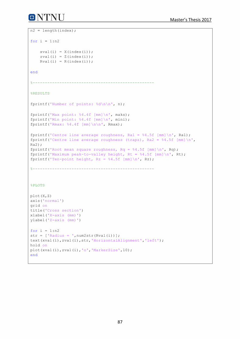
Master’s Thesis 2017
87
n2 = length(index);
for i = 1:n2
xval(i) = X(index(i)); zval(i) = Z(index(i)); Rval(i) = R(index(i));
end
%--------------------------------------------------
%RESULTS
fprintf('Number of points: %d\n\n', n);
fprintf('Max point: %4.4f [mm]\n', maks); fprintf('Min point: %4.4f [mm]\n', mini); fprintf('Rmax: %4.4f [mm]\n\n', Rmax);
fprintf('Centre line average roughness, Ra1 = %4.5f [mm]\n', Ra1); fprintf('Centre line average roughness (trapz), Ra2 = %4.5f [mm]\n',
Ra2); fprintf('Root mean square roughness, Rq = %4.5f [mm]\n', Rq); fprintf('Maximum peak-to-valley height, Rt = %4.5f [mm]\n', Rt);
fprintf('Ten-point height, Rz = %4.5f [mm]\n', Rz);
%--------------------------------------------------
%PLOTS
plot(X,Z) axis('normal') grid on title('Cross section') xlabel('X-axis (mm)')
ylabel('Z-axis (mm)')
for i = 1:n2 str = ['Radius = ',num2str(Rval(i))]; text(xval(i),zval(i),str,'HorizontalAlignment','left'); hold on plot(xval(i),zval(i),'o','MarkerSize',10); end
Related Documents