HAL Id: tel-01883642 https://tel.archives-ouvertes.fr/tel-01883642 Submitted on 28 Sep 2018 HAL is a multi-disciplinary open access archive for the deposit and dissemination of sci- entific research documents, whether they are pub- lished or not. The documents may come from teaching and research institutions in France or abroad, or from public or private research centers. L’archive ouverte pluridisciplinaire HAL, est destinée au dépôt et à la diffusion de documents scientifiques de niveau recherche, publiés ou non, émanant des établissements d’enseignement et de recherche français ou étrangers, des laboratoires publics ou privés. Numerical and experimental study of misaligned and wavy mechanical face seals operating under pressure pulses and pressure inversions Jérémy Cochain To cite this version: Jérémy Cochain. Numerical and experimental study of misaligned and wavy mechanical face seals operating under pressure pulses and pressure inversions. Mechanical engineering [physics.class-ph]. Université de Poitiers, 2018. English. NNT : 2018POIT2271. tel-01883642

Welcome message from author
This document is posted to help you gain knowledge. Please leave a comment to let me know what you think about it! Share it to your friends and learn new things together.
Transcript
HAL Id: tel-01883642https://tel.archives-ouvertes.fr/tel-01883642
Submitted on 28 Sep 2018
HAL is a multi-disciplinary open accessarchive for the deposit and dissemination of sci-entific research documents, whether they are pub-lished or not. The documents may come fromteaching and research institutions in France orabroad, or from public or private research centers.
L’archive ouverte pluridisciplinaire HAL, estdestinée au dépôt et à la diffusion de documentsscientifiques de niveau recherche, publiés ou non,émanant des établissements d’enseignement et derecherche français ou étrangers, des laboratoirespublics ou privés.
Numerical and experimental study of misaligned andwavy mechanical face seals operating under pressure
pulses and pressure inversionsJérémy Cochain
To cite this version:Jérémy Cochain. Numerical and experimental study of misaligned and wavy mechanical face sealsoperating under pressure pulses and pressure inversions. Mechanical engineering [physics.class-ph].Université de Poitiers, 2018. English. NNT : 2018POIT2271. tel-01883642
Annee 2018
THESE
Pour l’obtention du Grade de
Docteur de l’Universite de Poitiers
(Faculte des Sciences Fondamentales et Appliquees)(Diplome National - Arrete du 25 mai 2016)
ECOLE DOCTORALE :Sciences et Ingenierie en Materiaux, Mecanique, Energetique et Aeronautique
Secteur de Recherche :Genie mecanique, Productique, Transport
Presentee par :
Jeremy COCHAIN
Numerical and experimental study of misaligned andwavy mechanical face seals operating under pressure
pulses and inversions
Directeur de these : Noel BRUNETIERE
Soutenue le 31 Mai 2018devant la Commission d’Examen
JURY
Rapporteurs : M. Khonsari Professor, Louisiana State UniversityW. Seemann Professor, Karlsruher Institut fur Technologie
Examinateurs : J. Cayer-Barrioz Directeur de recherche, Ecole Centrale de Lyon, LTDSN. Brunetiere Chercheur, CNRS, Institut PprimeA. Parry Ingenieur, Schlumberger, ClamartA. Maoui Ingenieur, Cetim, Nantes
President : M. Arghir Professeur, Universite de Poitiers, Institut Pprime

2
3
Abstract
Face seals are mechanical devices used to seal rotating shafts in numerous applications. While they can operateefficiently under steady conditions for years, they tend to fail prematurely when operating in severe, or rapidlyvarying conditions. The focus of this research is the development and use of an experimental and a numericalmethod to investigate the impact of pressure pulses, pressure inversions and induced dynamic loading on theperformance of mechanical face seals exhibiting face misalignment and waviness.
The fluid solver of a state-of-the art face seal numerical model was extended to transient conditions and amodule for solving the dynamics for the axial and angular degrees of freedom of a flexibly-mounted statorwas added. A system-level experimental setup generating pressure pulses was instrumented and methods tocharacterise the performance of the face seal in terms of oil volume loss and ingression of water outer-fluidwere selected and implemented.
Face seals, with flat and misaligned faces, operating under pressure pulses and pressure inversions were exper-imentally tested and simulated. They showed only slight increase of water in the oil, no proportional increasewith time, and no measurable oil leakage. The low water ingression is due to the low film thickness combinedwith the short duration of the pressure inversions. An exploratory face seal of high waviness was also experi-mentally tested. Contrary to the other parameters, the waviness appears to significantly increase the leakageand promote water ingression and could thus be at the origin of some seal failures.
Resume
Les garnitures mecaniques sont utilisees dans de multiples applications pour realiser l’etancheite autour d’arbresen rotation. Ces composants peuvent fonctionner efficacement pendant plusieurs annees en conditions stables,mais leur duree de vie est significativement reduite lorsque les conditions varient. L’objectif de ce travailde recherche est de developper et d’utiliser un banc d’essais et un code de calcul pour etudier l’impact depulsations de pression, d’inversions de pression et du chargement dynamique resultant sur les performances degarnitures mecaniques ayant des faces mesalignees et presentant des defauts de planeite.
Le solveur fluide d’un modele numerique de garnitures mecaniques a ete etendu aux conditions transitoires.Un module resolvant la dynamique des forces et des moments a ete ajoute afin de predire le deplacement axialet les deplacements angulaires de la face montee de maniere flexible. Afin de caracteriser les performances degarnitures, un banc d’essais generant des pulsations de pression a ete instrumente et des methodes de mesurede perte de volume d’huile et d’entree d’eau mises en place
Des garnitures mecaniques a faces paralleles puis mesalignees, fonctionnant sous pulsations et inversions depression, ont ete testees experimentalement et simulees. Seules de tres faibles augmentations d’eau dans l’huileont ete observees, sans augmentation proportionnelle avec le temps, et sans fuite d’huile mesurable. Les faiblesvaleurs d’entrees d’eau sont dues a la faible epaisseur de film et a la courte duree des inversions de pression.Une garniture mecanique experimentale a fort defaut de planeite a aussi ete testee. Contrairement aux autresparametres, le defaut de planeite semble augmenter significativement la fuite et promouvoir les entrees d’eauet pourrait ainsi etre a l’origine de certaines defaillances.

4

5
Aknowledgement
Firstly, I would like to offer a sincere thanks to my supervisor, Noel Brunetiere, for his guidance and technicalhelp throughout my PhD. He is an exceptional supervisor both on the technical and relational aspects. I feelprivileged to have done my PhD under his guidance.I am also very grateful to the people of the department for our insightful discussions as well as for providinga friendly work environment.
In addition, I would like to thank the engineers and technicians of the Cetim sealing lab in Nantes for theirpractical help and collaboration.
Further, I wish to express my profound appreciation to all my colleagues, engineers, managers, advisors fortheir support and advice, especially to Guillaume, Andrea, Nicolas, Roel, Martin, Yves, Eric, Frederic, Jakub,Peter.In particular, I would like to deeply thank Henri for his resolute support, technical advice, and for helping meto connect my project to the broader context. Also, I would like to thank Andrew for being such a nice officeco-worker, for his technical support, and insightful reviews.
Lastly, I would like to thank my family and friends for their continuous support.

6
Contents
Nomenclature 11
Introduction 15
1 State of the art 191.1 Face seal basics . . . . . . . . . . . . . . . . . . . . . . . . . . . . . . . . . . . . . . . . . . . . . 20
1.1.1 Components . . . . . . . . . . . . . . . . . . . . . . . . . . . . . . . . . . . . . . . . . . 201.1.2 Design specifications . . . . . . . . . . . . . . . . . . . . . . . . . . . . . . . . . . . . . . 201.1.3 Operating principles - Phenomenology . . . . . . . . . . . . . . . . . . . . . . . . . . . . 211.1.4 Elementary equations . . . . . . . . . . . . . . . . . . . . . . . . . . . . . . . . . . . . . 211.1.5 General design considerations . . . . . . . . . . . . . . . . . . . . . . . . . . . . . . . . . 24
1.2 Review of face seals operating under severe transient conditions . . . . . . . . . . . . . . . . . . 261.2.1 Vibrations and misalignments . . . . . . . . . . . . . . . . . . . . . . . . . . . . . . . . . 261.2.2 Unsteady thermal effects . . . . . . . . . . . . . . . . . . . . . . . . . . . . . . . . . . . . 291.2.3 Pressure variations and pressure inversions . . . . . . . . . . . . . . . . . . . . . . . . . 311.2.4 Effect of face waviness . . . . . . . . . . . . . . . . . . . . . . . . . . . . . . . . . . . . . 321.2.5 Mixed lubrication . . . . . . . . . . . . . . . . . . . . . . . . . . . . . . . . . . . . . . . 331.2.6 Conclusions from the literature review . . . . . . . . . . . . . . . . . . . . . . . . . . . . 35
1.3 Summary of the state of the art . . . . . . . . . . . . . . . . . . . . . . . . . . . . . . . . . . . . 36
2 Face seal modelling 372.1 Modelling strategy and model building . . . . . . . . . . . . . . . . . . . . . . . . . . . . . . . . 372.2 The continuous equations . . . . . . . . . . . . . . . . . . . . . . . . . . . . . . . . . . . . . . . 39
2.2.1 Face kinematic description . . . . . . . . . . . . . . . . . . . . . . . . . . . . . . . . . . . 392.2.2 Axial and angular balance of a flexibly mounted stator . . . . . . . . . . . . . . . . . . . 422.2.3 Reynolds equation . . . . . . . . . . . . . . . . . . . . . . . . . . . . . . . . . . . . . . . 452.2.4 Contact model . . . . . . . . . . . . . . . . . . . . . . . . . . . . . . . . . . . . . . . . . 482.2.5 Energy equations and thermo-mechanical deformation equations . . . . . . . . . . . . . 492.2.6 Coupling strategies . . . . . . . . . . . . . . . . . . . . . . . . . . . . . . . . . . . . . . . 512.2.7 Closing remarks . . . . . . . . . . . . . . . . . . . . . . . . . . . . . . . . . . . . . . . . 52
2.3 Discrete equations . . . . . . . . . . . . . . . . . . . . . . . . . . . . . . . . . . . . . . . . . . . 532.3.1 Spatial discretisation using the finite element method . . . . . . . . . . . . . . . . . . . 532.3.2 Time integration schemes . . . . . . . . . . . . . . . . . . . . . . . . . . . . . . . . . . . 58
2.4 Numerical algorithms . . . . . . . . . . . . . . . . . . . . . . . . . . . . . . . . . . . . . . . . . 632.4.1 Non-linear algorithm for the Reynolds equation . . . . . . . . . . . . . . . . . . . . . . . 632.4.2 Non-linear algorithm for the axial and angular force balance solver . . . . . . . . . . . . 652.4.3 Closing remarks . . . . . . . . . . . . . . . . . . . . . . . . . . . . . . . . . . . . . . . . 672.4.4 Code workflow . . . . . . . . . . . . . . . . . . . . . . . . . . . . . . . . . . . . . . . . . 68
2.5 Summary of the face seal modelling strategy . . . . . . . . . . . . . . . . . . . . . . . . . . . . . 70
3 Comparison of the numerical model with published results 713.1 Verification of the axial and angular balance solver . . . . . . . . . . . . . . . . . . . . . . . . . 72
3.1.1 Characterisation of misaligned face seals . . . . . . . . . . . . . . . . . . . . . . . . . . . 723.1.2 Comparison with the analytical model of Green and Etsion . . . . . . . . . . . . . . . . 723.1.3 Comparison with the dynamic tracking model of Person et al. . . . . . . . . . . . . . . . 743.1.4 Verification with the dynamic model of Tournerie and Frene . . . . . . . . . . . . . . . . 763.1.5 Conclusions about the verification of the dynamic solver . . . . . . . . . . . . . . . . . . 77
3.2 Verification of the thermal and deformation solver . . . . . . . . . . . . . . . . . . . . . . . . . 78
7
8 CONTENTS
3.2.1 Verification of the thermal deformations . . . . . . . . . . . . . . . . . . . . . . . . . . . 783.2.2 Verification of unsteady thermal deformations . . . . . . . . . . . . . . . . . . . . . . . . 803.2.3 Conclusion about the verification of the thermal solver . . . . . . . . . . . . . . . . . . . 81
3.3 Comparison to the experimental data of Adjemout . . . . . . . . . . . . . . . . . . . . . . . . . 823.4 Summary of the numerical model verification and validation . . . . . . . . . . . . . . . . . . . . 83
4 Experimental test setup 854.1 System description . . . . . . . . . . . . . . . . . . . . . . . . . . . . . . . . . . . . . . . . . . . 86
4.1.1 Industrial test setup . . . . . . . . . . . . . . . . . . . . . . . . . . . . . . . . . . . . . . 864.1.2 Face seal holder . . . . . . . . . . . . . . . . . . . . . . . . . . . . . . . . . . . . . . . . . 864.1.3 Face seal . . . . . . . . . . . . . . . . . . . . . . . . . . . . . . . . . . . . . . . . . . . . 87
4.2 Instrumentation . . . . . . . . . . . . . . . . . . . . . . . . . . . . . . . . . . . . . . . . . . . . . 894.2.1 Measure of the volume of fluid in the reservoir . . . . . . . . . . . . . . . . . . . . . . . 894.2.2 Measurements of the inner and outer pressures of the face seal . . . . . . . . . . . . . . 904.2.3 Measurement of water ingression . . . . . . . . . . . . . . . . . . . . . . . . . . . . . . . 90
4.3 Setup characterisation . . . . . . . . . . . . . . . . . . . . . . . . . . . . . . . . . . . . . . . . . 924.3.1 Emergency shut-down . . . . . . . . . . . . . . . . . . . . . . . . . . . . . . . . . . . . . 924.3.2 Temperature . . . . . . . . . . . . . . . . . . . . . . . . . . . . . . . . . . . . . . . . . . 924.3.3 Pressure . . . . . . . . . . . . . . . . . . . . . . . . . . . . . . . . . . . . . . . . . . . . . 924.3.4 Rotational speed . . . . . . . . . . . . . . . . . . . . . . . . . . . . . . . . . . . . . . . . 924.3.5 Operating test conditions . . . . . . . . . . . . . . . . . . . . . . . . . . . . . . . . . . . 934.3.6 Face seal pressure difference . . . . . . . . . . . . . . . . . . . . . . . . . . . . . . . . . . 93
4.4 Test procedure . . . . . . . . . . . . . . . . . . . . . . . . . . . . . . . . . . . . . . . . . . . . . 974.5 Summary of the experimental test setup . . . . . . . . . . . . . . . . . . . . . . . . . . . . . . . 98
5 Numerical and experimental results 995.1 Face seal parameters and reference conditions . . . . . . . . . . . . . . . . . . . . . . . . . . . . 100
5.1.1 Geometry definition . . . . . . . . . . . . . . . . . . . . . . . . . . . . . . . . . . . . . . 1005.1.2 Parameters of the reference face seal . . . . . . . . . . . . . . . . . . . . . . . . . . . . . 1015.1.3 Face seal performance in reference conditions . . . . . . . . . . . . . . . . . . . . . . . . 101
5.2 Parametric study . . . . . . . . . . . . . . . . . . . . . . . . . . . . . . . . . . . . . . . . . . . . 1045.2.1 Impact of uncertainties of the inputs on the numerical predictions . . . . . . . . . . . . 1045.2.2 Impact of the operating conditions on numerical predictions . . . . . . . . . . . . . . . . 1085.2.3 Simulations of accelerations with transient thermal effects . . . . . . . . . . . . . . . . . 1105.2.4 Modelling simplifications and numerical considerations . . . . . . . . . . . . . . . . . . 112
5.3 Effect of pressure pulses . . . . . . . . . . . . . . . . . . . . . . . . . . . . . . . . . . . . . . . . 1135.3.1 Experimental results with pressure pulses . . . . . . . . . . . . . . . . . . . . . . . . . . 1135.3.2 Simulations with pressure pulses . . . . . . . . . . . . . . . . . . . . . . . . . . . . . . . 1145.3.3 Conclusions from the study of pressure pulses . . . . . . . . . . . . . . . . . . . . . . . . 121
5.4 Effect of rotor misalignment . . . . . . . . . . . . . . . . . . . . . . . . . . . . . . . . . . . . . . 1225.4.1 Experimental results with rotor misalignment and pressure pulses . . . . . . . . . . . . 1225.4.2 Simulations with a misaligned rotor . . . . . . . . . . . . . . . . . . . . . . . . . . . . . 1235.4.3 Simulation with a rotor misalignment of 3.5 mrad and pressure pulses . . . . . . . . . . 1275.4.4 Conclusions from the study of the face seal with rotor misalignment . . . . . . . . . . . 129
5.5 Effect of waviness . . . . . . . . . . . . . . . . . . . . . . . . . . . . . . . . . . . . . . . . . . . . 1305.5.1 Experimental results for the wavy face seal prototype under pressure pulses . . . . . . . 1305.5.2 Simulation of the reference face seal with consideration of waviness . . . . . . . . . . . . 1325.5.3 Simulation of the reference face seal with waviness and with pressure pulses . . . . . . . 1415.5.4 Simulation of the wavy face seal prototype . . . . . . . . . . . . . . . . . . . . . . . . . 1425.5.5 Conclusions from the study of the effect of face waviness . . . . . . . . . . . . . . . . . . 144
5.6 Summary of the main results of the studies and conclusion . . . . . . . . . . . . . . . . . . . . . 1455.6.1 Summary of the main results . . . . . . . . . . . . . . . . . . . . . . . . . . . . . . . . . 1455.6.2 Conclusions from the experimental and numerical studies . . . . . . . . . . . . . . . . . 146
Conclusion and outlook 147
A Appendix 149A.1 Transformation from material to reference coordinates . . . . . . . . . . . . . . . . . . . . . . . 149A.2 Derivation of the Reynolds equation . . . . . . . . . . . . . . . . . . . . . . . . . . . . . . . . . 151A.3 Contact model sensitivity . . . . . . . . . . . . . . . . . . . . . . . . . . . . . . . . . . . . . . . 155

CONTENTS 9
A.4 Semi-Discrete form of the energy equation . . . . . . . . . . . . . . . . . . . . . . . . . . . . . . 157A.5 Semi-Discrete form of the deformation equation . . . . . . . . . . . . . . . . . . . . . . . . . . . 158A.6 Data used for the verification of the dynamic solver . . . . . . . . . . . . . . . . . . . . . . . . . 159A.7 Data used for the verification of the thermo-mechanical solver . . . . . . . . . . . . . . . . . . . 161A.8 Data used for the comparison with Adjemout . . . . . . . . . . . . . . . . . . . . . . . . . . . . 162A.9 Impact of number of nodes and length of the time step for the axial and angular solver . . . . . 164A.10 Memento on measures of flow . . . . . . . . . . . . . . . . . . . . . . . . . . . . . . . . . . . . . 165A.11 Additional measurements investigated . . . . . . . . . . . . . . . . . . . . . . . . . . . . . . . . 166
List of figures 167
List of tables 170
Bibliography 173

10 CONTENTS
Nomenclature
Continuous variables
Symbol Description Unit
a, b, c Coordinates of a material point of a face . . . . . . . ma Acceleration vector . . . . . . . . . . . . . . . . . . . . . . . . . . . . m/s2
a, b Contact model coefficients . . . . . . . . . . . . . . . . . . . . .A Amplitude of pressure signal . . . . . . . . . . . . . . . . . . . PaAw Waviness amplitude . . . . . . . . . . . . . . . . . . . . . . . . . . . mB Balance ratio . . . . . . . . . . . . . . . . . . . . . . . . . . . . . . . . . .bvisc Thermo-viscosity coefficient . . . . . . . . . . . . . . . . . . . 1/ KC Face centre distance . . . . . . . . . . . . . . . . . . . . . . . . . . . mC0 Designed face centre distance . . . . . . . . . . . . . . . . . . mCp Heat capacity . . . . . . . . . . . . . . . . . . . . . . . . . . . . . . . . . J/(K · kg)Cj−1 Parameters for axial and angular balance solverD Dimensionless damping coefficient . . . . . . . . . . . . .d Damping . . . . . . . . . . . . . . . . . . . . . . . . . . . . . . . . . . . . . . Ns/mD Seal diameter . . . . . . . . . . . . . . . . . . . . . . . . . . . . . . . . . me Face seal ring thickness . . . . . . . . . . . . . . . . . . . . . . . . mE Young’s modulus . . . . . . . . . . . . . . . . . . . . . . . . . . . . . . PaE′ Equivalent Young’s modulus . . . . . . . . . . . . . . . . . . . Paf Friction coefficient . . . . . . . . . . . . . . . . . . . . . . . . . . . . .f Frequency of pressure signal . . . . . . . . . . . . . . . . . . . HzF Force . . . . . . . . . . . . . . . . . . . . . . . . . . . . . . . . . . . . . . . . . . NFz dimensionless axial force . . . . . . . . . . . . . . . . . . . . . . .G Duty parameter . . . . . . . . . . . . . . . . . . . . . . . . . . . . . . .h Film thickness . . . . . . . . . . . . . . . . . . . . . . . . . . . . . . . . . mhc Heat convection coefficient . . . . . . . . . . . . . . . . . . . . W/K ·m2
K Dimensionless stiffness coefficient . . . . . . . . . . . . . .Khydraulic Factor for film thickness shape . . . . . . . . . . . . . . . .k Stiffness . . . . . . . . . . . . . . . . . . . . . . . . . . . . . . . . . . . . . . . N/mk Heat conductivity . . . . . . . . . . . . . . . . . . . . . . . . . . . . . W/mK Compliance matrix . . . . . . . . . . . . . . . . . . . . . . . . . . . .I Support inertia coefficient . . . . . . . . . . . . . . . . . . . . . kg ·m2
I Dimensionless support inertia coefficient . . . . . . .L Axial position of the face centre . . . . . . . . . . . . . . . m
Le Upwinding function . . . . . . . . . . . . . . . . . . . . . . . . . . .M Moment . . . . . . . . . . . . . . . . . . . . . . . . . . . . . . . . . . . . . . . N ·mm Mass . . . . . . . . . . . . . . . . . . . . . . . . . . . . . . . . . . . . . . . . . . kgm Fluid mass flow . . . . . . . . . . . . . . . . . . . . . . . . . . . . . . . kg/sm Dimensionless mass . . . . . . . . . . . . . . . . . . . . . . . . . . . .µ Fluid viscosity . . . . . . . . . . . . . . . . . . . . . . . . . . . . . . . . . Pa · sNu Nusselt number . . . . . . . . . . . . . . . . . . . . . . . . . . . . . . .nx, ny Unit vector normal to the film surface . . . . . . . . .O Origin of the reference frame . . . . . . . . . . . . . . . . . .
11
12 CONTENTS
Continuous variables
Symbol Description Unit
p Pressure . . . . . . . . . . . . . . . . . . . . . . . . . . . . . . . Papc Contact pressure vector . . . . . . . . . . . . . . . . Papφ Oil overpressure offset . . . . . . . . . . . . . . . . . PaP Dissipated power . . . . . . . . . . . . . . . . . . . . . . WPr Prandtl number . . . . . . . . . . . . . . . . . . . . . . .Q Flow rate or leakage . . . . . . . . . . . . . . . . . . . m3/sq Heat flux per unit surface . . . . . . . . . . . . . . W/m2
r Radius . . . . . . . . . . . . . . . . . . . . . . . . . . . . . . . . mrgas Gas constant for air . . . . . . . . . . . . . . . . . . . J/(K · kg)Re Reynolds number . . . . . . . . . . . . . . . . . . . . . .R, S Rotor and stator material point . . . . . . . .R0 Absolute reference frame . . . . . . . . . . . . . . .
R′′
Rotating reference frame . . . . . . . . . . . . . . .R Average asperity radius . . . . . . . . . . . . . . . . mS Seal surface . . . . . . . . . . . . . . . . . . . . . . . . . . . . m2
Sq Standard deviation of surface roughness mS Pressure signal . . . . . . . . . . . . . . . . . . . . . . . . Pat Time . . . . . . . . . . . . . . . . . . . . . . . . . . . . . . . . . . s∆t Time step duration . . . . . . . . . . . . . . . . . . . . stcharac Characteristic time . . . . . . . . . . . . . . . . . . . . sT Torque . . . . . . . . . . . . . . . . . . . . . . . . . . . . . . . . N ·mT Temperature . . . . . . . . . . . . . . . . . . . . . . . . . . . Ku Displacement vector . . . . . . . . . . . . . . . . . . .u, v, w Fluid velocities . . . . . . . . . . . . . . . . . . . . . . . . m/sU, V Face velocities in Cartesien coordinates m/sV Tangential speed . . . . . . . . . . . . . . . . . . . . . . . m/sV Volume of the sealing interface . . . . . . . . . m3
x, y Coordinates of a point in the film . . . . . . mX, Y, Z Unit vectors . . . . . . . . . . . . . . . . . . . . . . . . . . .z Face centre distance . . . . . . . . . . . . . . . . . . . m
Symbol Description Unitαε Upwinding coefficient . . . . . . . . . . . . . . . . . . . . . . . . . . . . . . .α thermal expansion coefficient . . . . . . . . . . . . . . . . . . . . . . .β Taper or coning angle . . . . . . . . . . . . . . . . . . . . . . . . . . . . . . radγ Dimensionless relative misalignment . . . . . . . . . . . . . . . .γ0 Dimensionless relative misalignment due to rotor tiltδ Taper ratio . . . . . . . . . . . . . . . . . . . . . . . . . . . . . . . . . . . . . . . . .ε Strain tensor . . . . . . . . . . . . . . . . . . . . . . . . . . . . . . . . . . . . . . .ζ, η Coordinates in iso-parametric representation . . . . . . . .ζ Cumulative volume of fluid entering/leaving the seal %θ Generalized theta parameter . . . . . . . . . . . . . . . . . . . . . . . .ϑ Arbitrary weight function . . . . . . . . . . . . . . . . . . . . . . . . . .η Number of asperity peaks per unit square area . . . . . . m−2
θ Face angular position . . . . . . . . . . . . . . . . . . . . . . . . . . . . . . . radλ Gas mass fraction . . . . . . . . . . . . . . . . . . . . . . . . . . . . . . . . . .λ, µ Lame parameters . . . . . . . . . . . . . . . . . . . . . . . . . . . . . . . . . . . Paλ Surface correlation length . . . . . . . . . . . . . . . . . . . . . . . . . . m

CONTENTS 13
Continuous variables
Symbol Description Unitσs Standard deviation of the heights of the summits of the asperities mρ Density . . . . . . . . . . . . . . . . . . . . . . . . . . . . . . . . . . . . . . . . . . . . . . . . . . . . . . . . . kg/m3
ς, γ Newmark scheme parameter . . . . . . . . . . . . . . . . . . . . . . . . . . . . . . . . . . . . .σ Stress tensor . . . . . . . . . . . . . . . . . . . . . . . . . . . . . . . . . . . . . . . . . . . . . . . . . . . . N/m2
τ Delay in pressure signals . . . . . . . . . . . . . . . . . . . . . . . . . . . . . . . . . . . . . . . . sτ Shear stress . . . . . . . . . . . . . . . . . . . . . . . . . . . . . . . . . . . . . . . . . . . . . . . . . . . . . N/m2
φ Phase angle . . . . . . . . . . . . . . . . . . . . . . . . . . . . . . . . . . . . . . . . . . . . . . . . . . . . . radχ Misalignment angle . . . . . . . . . . . . . . . . . . . . . . . . . . . . . . . . . . . . . . . . . . . . . . radω Rotational speed . . . . . . . . . . . . . . . . . . . . . . . . . . . . . . . . . . . . . . . . . . . . . . . . rad/sΩ Domain . . . . . . . . . . . . . . . . . . . . . . . . . . . . . . . . . . . . . . . . . . . . . . . . . . . . . . . . .∂Ω Domain boundary . . . . . . . . . . . . . . . . . . . . . . . . . . . . . . . . . . . . . . . . . . . . . . .
Discrete variables
Symbol Descriptionnnode Number of nodesKij Stiffness matrixbi RHS vectorfi Source and boundary vectorTj Nodal temperaturer Residual vectorHij , Mij Thermal and mechanical influence coefficientsui Displacement at node ipj Nodal pressureNj Shape functionJ Jacobian matrix
Subscripts and Superscripts
Subscript or Superscript Descriptionc contacti innero outerh hydraulicav averagedry dryvisc viscousr, 1 rotors, 2 statorf fluidx along x axisy along y axisg gasl liquidPROD Product upwind schemer Element-wiseT Transposetj At time instant tj
k At kth iteration

14 CONTENTS
Introduction
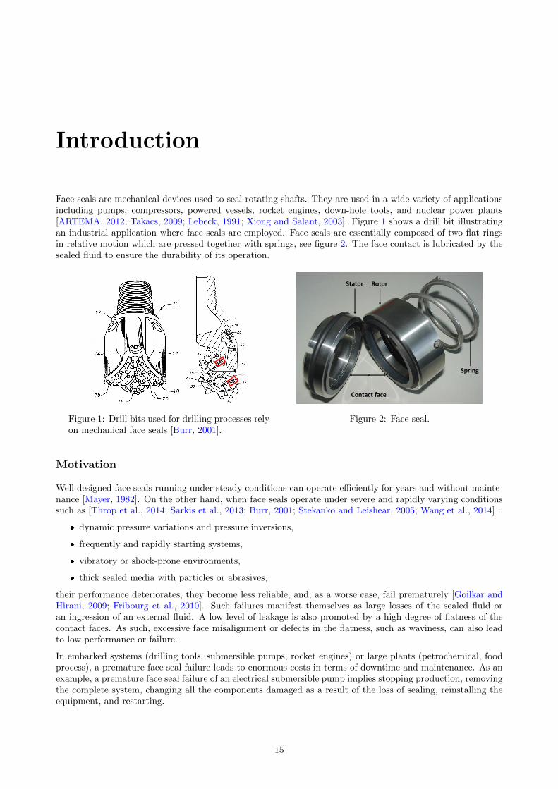
Face seals are mechanical devices used to seal rotating shafts. They are used in a wide variety of applicationsincluding pumps, compressors, powered vessels, rocket engines, down-hole tools, and nuclear power plants[ARTEMA, 2012; Takacs, 2009; Lebeck, 1991; Xiong and Salant, 2003]. Figure 1 shows a drill bit illustratingan industrial application where face seals are employed. Face seals are essentially composed of two flat ringsin relative motion which are pressed together with springs, see figure 2. The face contact is lubricated by thesealed fluid to ensure the durability of its operation.
Figure 1: Drill bits used for drilling processes relyon mechanical face seals [Burr, 2001].
RotorStator
Spring
Contact face
Figure 2: Face seal.
Motivation
Well designed face seals running under steady conditions can operate efficiently for years and without mainte-nance [Mayer, 1982]. On the other hand, when face seals operate under severe and rapidly varying conditionssuch as [Throp et al., 2014; Sarkis et al., 2013; Burr, 2001; Stekanko and Leishear, 2005; Wang et al., 2014] :
dynamic pressure variations and pressure inversions,
frequently and rapidly starting systems,
vibratory or shock-prone environments,
thick sealed media with particles or abrasives,
their performance deteriorates, they become less reliable, and, as a worse case, fail prematurely [Goilkar andHirani, 2009; Fribourg et al., 2010]. Such failures manifest themselves as large losses of the sealed fluid oran ingression of an external fluid. A low level of leakage is also promoted by a high degree of flatness of thecontact faces. As such, excessive face misalignment or defects in the flatness, such as waviness, can also leadto low performance or failure.
In embarked systems (drilling tools, submersible pumps, rocket engines) or large plants (petrochemical, foodprocess), a premature face seal failure leads to enormous costs in terms of downtime and maintenance. As anexample, a premature face seal failure of an electrical submersible pump implies stopping production, removingthe complete system, changing all the components damaged as a result of the loss of sealing, reinstalling theequipment, and restarting.
15
16 CONTENTS
The true root causes of a face seal failure are often difficult to identify, as many components are damaged andbecause of the overall complexity of the system and of the face seals themselves. In this regard, three actionsare generally undertaken on a short-term basis in the industry [Merrill and Dwiggins, 2017] :
Place multiple face seals in series in case one or two fail. This increases the manufacturing and operatingcost.
Perform more regular maintenance and frequent changes of the seal. This increases the maintenance andsustaining cost.
Narrow the operating envelope of the product to less demanding conditions. This induces a financial lossas the operating market is reduced or production slowed down.
Taking into account the above information, the main industrial motivations to improve face seals operating insevere conditions are:
to reduce the total cost of ownership of the system,
to open up to yet inaccessible markets,
to increase system efficiency/production rate,
to reduce the occurrence of premature/catastrophic failure.
To illustrate, a step increase in face seal reliability may allow reducing the number of redundant seals in anelectrical submersible pump and therefore the total cost of ownership. The use of high temperature resistantsemi-dynamic seals in drilling tools may open up to high temperature markets. The choice of grooved facesmay allow higher rotating speeds in a process plan, thus leading to a higher production rate. A more robustdesign may resist unplanned events and avoid a catastrophic failure.
Moreover, the increase of face seal performance and reduction of failures help to preserve the environment bylimiting the leakage of the process fluids.
Industrial context
The behavior and performance of face seals are governed by coupled mechanisms, including: face lubrication,dynamic motion, heat generation, and thermo-mechanical deformations. Given this inherent complexity, bothnumerical simulations and experimental testing are relied upon to reduce the cost and time of the face sealimprovement process.
Numerical simulations help to:
Understand the behavior of the seal and the impact of varying the design parameters (closing force,geometrical dimensions, etc.).
Evaluate, in a timely manner, multiple designs to identify a reduced set of promising prototypes.
Conduct post-mortem analysis of past failures.
The level of confidence of the simulation results is directly related to the degree of verification and validation ofthe underlying models and algorithms. To be used as a good design tool, a numerical model needs a thoroughcomparison with (i) previously published results and (ii) experimental data.
Experimental tests allow subjecting the face seals to operating-like conditions and thus:
Comparing and validating promising prototypes,
Collect data for the validation of numerical models,
Reproducing operating failures to gain a better understanding of them.
Experimental tests for face seals generally provide only system level information, such as leakage, torque, andsurface topography. This information is, however, of limited use for the understanding of the internal behav-ior of the seal (lubrication regime, heat generation, etc.). Experimental campaigns also require substantialresources.
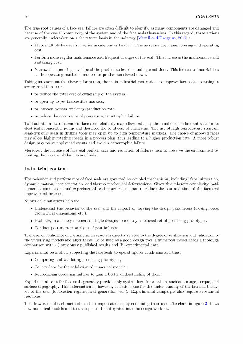
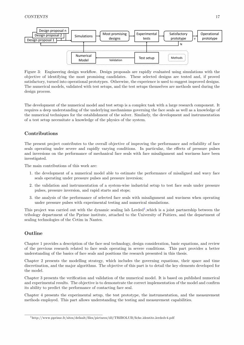
The drawbacks of each method can be compensated for by combining their use. The chart in figure 3 showshow numerical models and test setups can be integrated into the design workflow.
CONTENTS 17
Design proposal 1
Design proposal 2Design proposal n
SimulationsMost promising
designsExperimental
tests Operational prototype
Numerical Model
Test setupValidation
Satisfactory prototype
N
Y
Methods
Figure 3: Engineering design workflow. Design proposals are rapidly evaluated using simulations with theobjective of identifying the most promising candidates. These selected designs are tested and, if provedsatisfactory, turned into operational prototypes. Otherwise, the experience is used to suggest improved designs.The numerical models, validated with test setups, and the test setups themselves are methods used during thedesign process.
The development of the numerical model and test setup is a complex task with a large research component. Itrequires a deep understanding of the underlying mechanisms governing the face seals as well as a knowledge ofthe numerical techniques for the establishment of the solver. Similarly, the development and instrumentationof a test setup necessitate a knowledge of the physics of the system.
Contributions
The present project contributes to the overall objective of improving the performance and reliability of faceseals operating under severe and rapidly varying conditions. In particular, the effects of pressure pulsesand inversions on the performance of mechanical face seals with face misalignment and waviness have beeninvestigated.
The main contributions of this work are:
1. the development of a numerical model able to estimate the performance of misaligned and wavy faceseals operating under pressure pulses and pressure inversion;
2. the validation and instrumentation of a system-wise industrial setup to test face seals under pressurepulses, pressure inversion, and rapid starts and stops;
3. the analysis of the performance of selected face seals with misalignment and waviness when operatingunder pressure pulses with experimental testing and numerical simulations.
This project was carried out with the dynamic sealing lab Lerded1,which is a joint partnership between thetribology department of the Pprime institute, attached to the University of Poitiers, and the department ofsealing technologies of the Cetim in Nantes.
Outline
Chapter 1 provides a description of the face seal technology, design consideration, basic equations, and reviewof the previous research related to face seals operating in severe conditions. This part provides a betterunderstanding of the basics of face seals and positions the research presented in this thesis.
Chapter 2 presents the modelling strategy, which includes the governing equations, their space and timediscretisation, and the major algorithms. The objective of this part is to detail the key elements developed forthe model.
Chapter 3 presents the verification and validation of the numerical model. It is based on published numericaland experimental results. The objective is to demonstrate the correct implementation of the model and confirmits ability to predict the performance of contacting face seal.
Chapter 4 presents the experimental setup, the test prototype, the instrumentation, and the measurementmethods employed. This part allows understanding the testing and measurement capabilities.
1http://www.pprime.fr/sites/default/files/pictures/d3/TRIBOLUB/fiche identite lerdedv4.pdf

18 CONTENTS
Chapter 5 presents the numerical and experimental results of selected face seals operating under pressurepulses. The performance in terms of outer fluid ingression, leakage, and wear, depending on the misalignmentand waviness, are analysed.
Chapter 6 presents the main results of this research and suggests future developments.
Chapter 1
State of the art
The objective of this part is firstly to present the main components of mechanical face seals and their operatingprinciples. Elementary equations that may be used to obtain a first order of magnitude of the performance arealso presented. Secondly, a review of the studies pertaining to the operation of face seals in severe conditionswill be given.
Contents1.1 Face seal basics . . . . . . . . . . . . . . . . . . . . . . . . . . . . . . . . . . . . . . . 20
1.1.1 Components . . . . . . . . . . . . . . . . . . . . . . . . . . . . . . . . . . . . . . . . 20
1.1.2 Design specifications . . . . . . . . . . . . . . . . . . . . . . . . . . . . . . . . . . . . 20
1.1.3 Operating principles - Phenomenology . . . . . . . . . . . . . . . . . . . . . . . . . . 21
1.1.4 Elementary equations . . . . . . . . . . . . . . . . . . . . . . . . . . . . . . . . . . . 21
1.1.5 General design considerations . . . . . . . . . . . . . . . . . . . . . . . . . . . . . . . 24
1.2 Review of face seals operating under severe transient conditions . . . . . . . . . 26
1.2.1 Vibrations and misalignments . . . . . . . . . . . . . . . . . . . . . . . . . . . . . . . 26
1.2.2 Unsteady thermal effects . . . . . . . . . . . . . . . . . . . . . . . . . . . . . . . . . . 29
1.2.3 Pressure variations and pressure inversions . . . . . . . . . . . . . . . . . . . . . . . 31
1.2.4 Effect of face waviness . . . . . . . . . . . . . . . . . . . . . . . . . . . . . . . . . . . 32
1.2.5 Mixed lubrication . . . . . . . . . . . . . . . . . . . . . . . . . . . . . . . . . . . . . 33
1.2.6 Conclusions from the literature review . . . . . . . . . . . . . . . . . . . . . . . . . . 35
1.3 Summary of the state of the art . . . . . . . . . . . . . . . . . . . . . . . . . . . . 36
19
20 CHAPTER 1. STATE OF THE ART
1.1 Face seal basics
1.1.1 Components
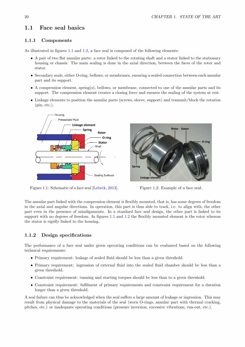
As illustrated in figures 1.1 and 1.2, a face seal is composed of the following elements:
A pair of two flat annular parts: a rotor linked to the rotating shaft and a stator linked to the stationaryhousing or chassis. The main sealing is done in the axial direction, between the faces of the rotor andstator.
Secondary seals, either O-ring, bellows, or membranes, ensuring a sealed connection between each annularpart and its support.
A compression element, spring(s), bellows, or membrane, connected to one of the annular parts and itssupport. The compression element creates a closing force and ensures the sealing of the system at rest.
Linkage elements to position the annular parts (screws, sleeve, support) and transmit/block the rotation(pin, etc.).
Rotor
Stator
O-ring
Spring
Linkage element
Figure 1.1: Schematic of a face seal [Lebeck, 2013].
Rotor Stator
Spring
O-ring
Linkage element
Figure 1.2: Example of a face seal.
The annular part linked with the compression element is flexibly mounted, that is, has some degrees of freedomin the axial and angular directions. In operation, this part is thus able to track, i.e. to align with, the otherpart even in the presence of misalignments. In a standard face seal design, the other part is linked to itssupport with no degrees of freedom. In figures 1.1 and 1.2 the flexibly mounted element is the rotor whereasthe stator is rigidly linked to the housing.
1.1.2 Design specifications
The performance of a face seal under given operating conditions can be evaluated based on the followingtechnical requirements:
Primary requirement: leakage of sealed fluid should be less than a given threshold.
Primary requirement: ingression of external fluid into the sealed fluid chamber should be less than agiven threshold.
Constraint requirement: running and starting torques should be less than to a given threshold.
Constraint requirement: fulfilment of primary requirements and constraint requirement for a durationlonger than a given threshold.
A seal failure can thus be acknowledged when the seal suffers a large amount of leakage or ingression. This mayresult from physical damage to the materials of the seal (worn O-rings, annular part with thermal cracking,pitches, etc.) or inadequate operating conditions (pressure inversion, excessive vibrations, run-out, etc.).
1.1. FACE SEAL BASICS 21
1.1.3 Operating principles - Phenomenology
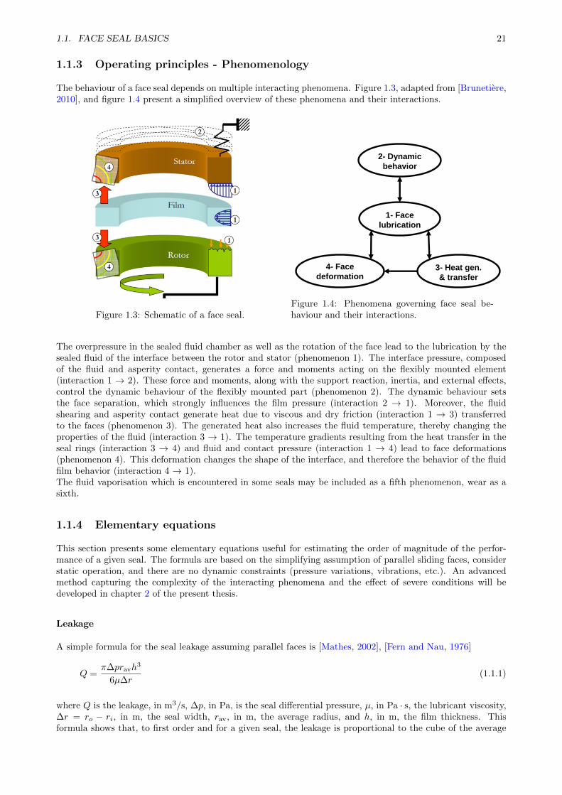
The behaviour of a face seal depends on multiple interacting phenomena. Figure 1.3, adapted from [Brunetiere,2010], and figure 1.4 present a simplified overview of these phenomena and their interactions.
Figure 1.3: Schematic of a face seal.
1- Face
lubrication
2- Dynamic
behavior
3- Heat gen.
& transfer
4- Face
deformation
Figure 1.4: Phenomena governing face seal be-haviour and their interactions.
The overpressure in the sealed fluid chamber as well as the rotation of the face lead to the lubrication by thesealed fluid of the interface between the rotor and stator (phenomenon 1). The interface pressure, composedof the fluid and asperity contact, generates a force and moments acting on the flexibly mounted element(interaction 1 → 2). These force and moments, along with the support reaction, inertia, and external effects,control the dynamic behaviour of the flexibly mounted part (phenomenon 2). The dynamic behaviour setsthe face separation, which strongly influences the film pressure (interaction 2 → 1). Moreover, the fluidshearing and asperity contact generate heat due to viscous and dry friction (interaction 1 → 3) transferredto the faces (phenomenon 3). The generated heat also increases the fluid temperature, thereby changing theproperties of the fluid (interaction 3 → 1). The temperature gradients resulting from the heat transfer in theseal rings (interaction 3 → 4) and fluid and contact pressure (interaction 1 → 4) lead to face deformations(phenomenon 4). This deformation changes the shape of the interface, and therefore the behavior of the fluidfilm behavior (interaction 4 → 1).The fluid vaporisation which is encountered in some seals may be included as a fifth phenomenon, wear as asixth.
1.1.4 Elementary equations
This section presents some elementary equations useful for estimating the order of magnitude of the perfor-mance of a given seal. The formula are based on the simplifying assumption of parallel sliding faces, considerstatic operation, and there are no dynamic constraints (pressure variations, vibrations, etc.). An advancedmethod capturing the complexity of the interacting phenomena and the effect of severe conditions will bedeveloped in chapter 2 of the present thesis.
Leakage
A simple formula for the seal leakage assuming parallel faces is [Mathes, 2002], [Fern and Nau, 1976]
Q =π∆pravh
3
6µ∆r(1.1.1)
where Q is the leakage, in m3/s, ∆p, in Pa, is the seal differential pressure, µ, in Pa · s, the lubricant viscosity,∆r = ro − ri, in m, the seal width, rav, in m, the average radius, and h, in m, the film thickness. Thisformula shows that, to first order and for a given seal, the leakage is proportional to the cube of the average
22 CHAPTER 1. STATE OF THE ART
film thickness, proportional to the pressure difference, and inversely proportional to the viscosity. All theparameters, except the film thickness, are known a priori. In practice the face seal film thickness varies alongthe radius and circumference, as it depends on the phenomena governing the behaviour of the seal. In the caseof parallel faces, asperity contact occurs and the film thickness can thus be considered as being on the orderof 3 to 5 times the standard deviation of the surface roughness, Sq.
Friction torque
The overall friction torque is due to energy dissipation from fluid viscous shearing and friction of the contactingasperities. An order of magnitude of the torque can be obtained using the formulas below, valid for parallelfaces [Brunetiere and Tournerie, 2016a]
T = Tvisc + Tdry (1.1.2)
with
Tvisc =πµω
h
r4o − r4
i
2(1.1.3)
Tdry = 2πfpcr3o − r3
i
3(1.1.4)
where f is the dry contact friction coefficient, ω, in rad/s, is the speed of rotation, and pc, in Pa, is an averagedseal contact pressure.
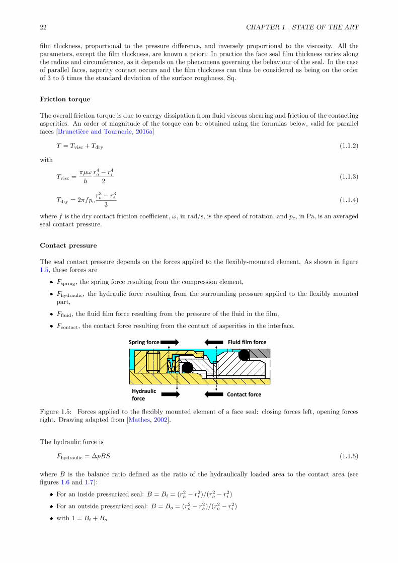
Contact pressure
The seal contact pressure depends on the forces applied to the flexibly-mounted element. As shown in figure1.5, these forces are
Fspring, the spring force resulting from the compression element,
Fhydraulic, the hydraulic force resulting from the surrounding pressure applied to the flexibly mountedpart,
Ffluid, the fluid film force resulting from the pressure of the fluid in the film,
Fcontact, the contact force resulting from the contact of asperities in the interface.
Spring force
Hydraulic force
Fluid film force
Contact force
Figure 1.5: Forces applied to the flexibly mounted element of a face seal: closing forces left, opening forcesright. Drawing adapted from [Mathes, 2002].
The hydraulic force is
Fhydraulic = ∆pBS (1.1.5)
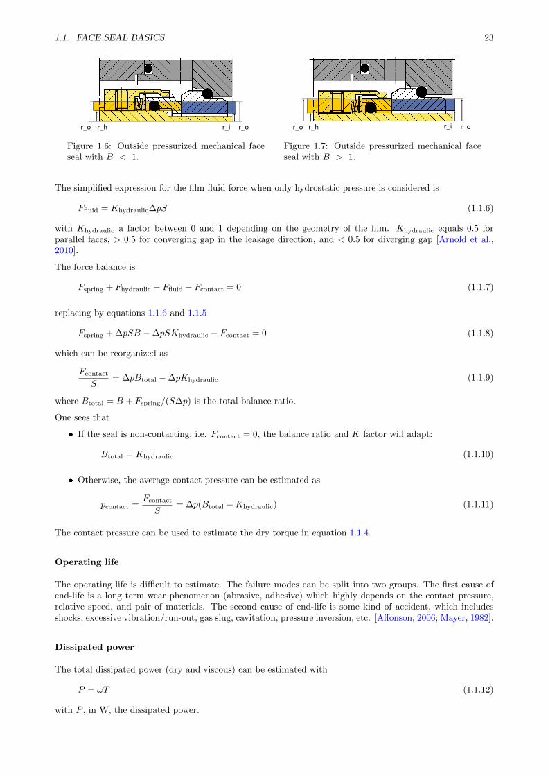
where B is the balance ratio defined as the ratio of the hydraulically loaded area to the contact area (seefigures 1.6 and 1.7):
For an inside pressurized seal: B = Bi = (r2h − r2
i )/(r2o − r2
i )
For an outside pressurized seal: B = Bo = (r2o − r2
h)/(r2o − r2
i )
with 1 = Bi +Bo
1.1. FACE SEAL BASICS 23
r_o r_h r_i r_o
Figure 1.6: Outside pressurized mechanical faceseal with B < 1.
r_o r_h r_i r_o
Figure 1.7: Outside pressurized mechanical faceseal with B > 1.
The simplified expression for the film fluid force when only hydrostatic pressure is considered is
Ffluid = Khydraulic∆pS (1.1.6)
with Khydraulic a factor between 0 and 1 depending on the geometry of the film. Khydraulic equals 0.5 forparallel faces, > 0.5 for converging gap in the leakage direction, and < 0.5 for diverging gap [Arnold et al.,2010].
The force balance is
Fspring + Fhydraulic − Ffluid − Fcontact = 0 (1.1.7)
replacing by equations 1.1.6 and 1.1.5
Fspring + ∆pSB −∆pSKhydraulic − Fcontact = 0 (1.1.8)
which can be reorganized as
Fcontact
S= ∆pBtotal −∆pKhydraulic (1.1.9)
where Btotal = B + Fspring/(S∆p) is the total balance ratio.
One sees that
If the seal is non-contacting, i.e. Fcontact = 0, the balance ratio and K factor will adapt:
Btotal = Khydraulic (1.1.10)
Otherwise, the average contact pressure can be estimated as
pcontact =Fcontact
S= ∆p(Btotal −Khydraulic) (1.1.11)
The contact pressure can be used to estimate the dry torque in equation 1.1.4.
Operating life
The operating life is difficult to estimate. The failure modes can be split into two groups. The first cause ofend-life is a long term wear phenomenon (abrasive, adhesive) which highly depends on the contact pressure,relative speed, and pair of materials. The second cause of end-life is some kind of accident, which includesshocks, excessive vibration/run-out, gas slug, cavitation, pressure inversion, etc. [Affonson, 2006; Mayer, 1982].
Dissipated power
The total dissipated power (dry and viscous) can be estimated with
P = ωT (1.1.12)
with P , in W, the dissipated power.
24 CHAPTER 1. STATE OF THE ART
Example
To illustrate, the face seal with parameters shown in table 1.1 is considered. The values are based on those ofthe seal studied in this work.
Table 1.1: Parameters of a face seal.
Parameters Symbol Unit ValueInner radius ri m 0.0114Outer radius ro m 0.0142Pressure difference ∆p Pa 1 · 105
Lubricant viscosity µ Pa · s 0.0078Surface roughness standard deviation Sq µm 0.21Balance ratio B 1.0Spring force Fspring N 125
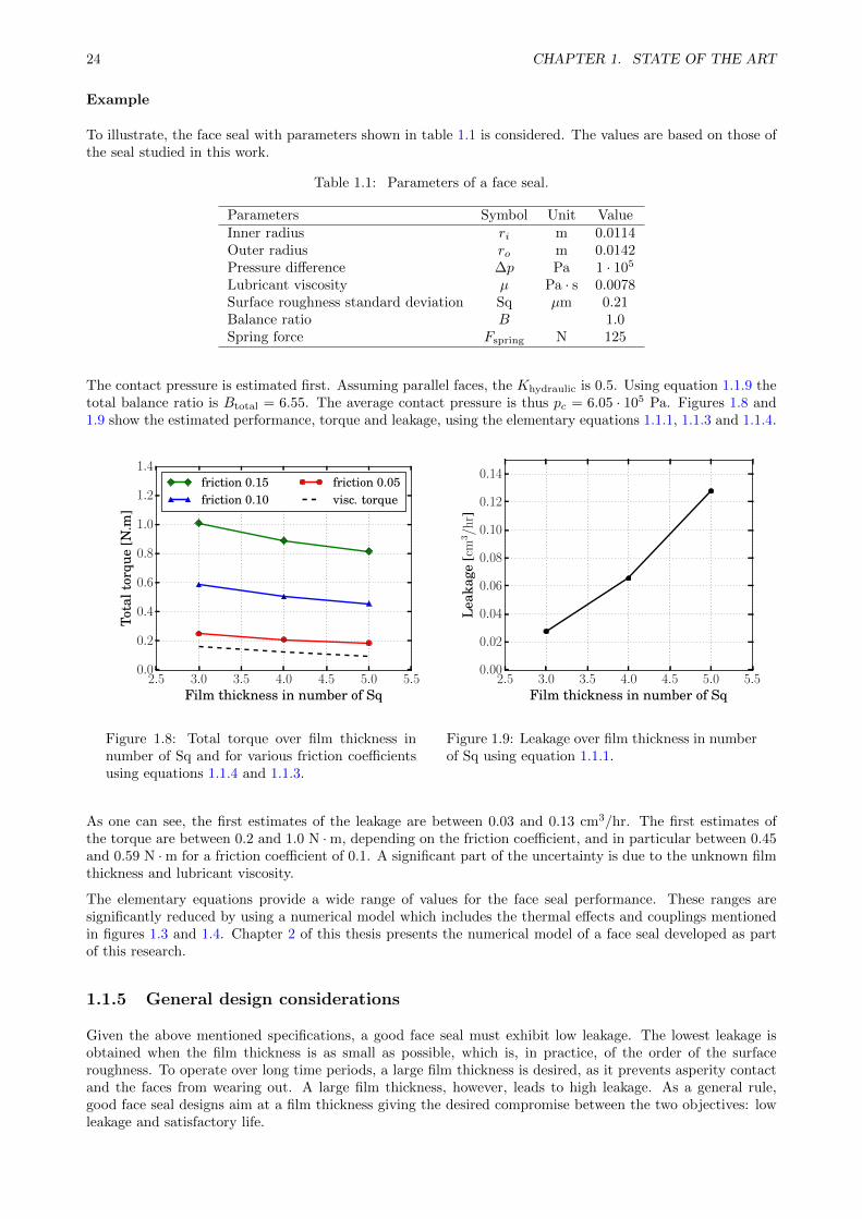
The contact pressure is estimated first. Assuming parallel faces, the Khydraulic is 0.5. Using equation 1.1.9 thetotal balance ratio is Btotal = 6.55. The average contact pressure is thus pc = 6.05 · 105 Pa. Figures 1.8 and1.9 show the estimated performance, torque and leakage, using the elementary equations 1.1.1, 1.1.3 and 1.1.4.
2.5 3.0 3.5 4.0 4.5 5.0 5.5Film thickness in number of Sq
0.0
0.2
0.4
0.6
0.8
1.0
1.2
1.4
Tota
ltor
que
[N.m
]
friction 0.15friction 0.10
friction 0.05visc. torque
Figure 1.8: Total torque over film thickness innumber of Sq and for various friction coefficientsusing equations 1.1.4 and 1.1.3.
2.5 3.0 3.5 4.0 4.5 5.0 5.5Film thickness in number of Sq
0.00
0.02
0.04
0.06
0.08
0.10
0.12
0.14L
eaka
ge[c
m3/h
r]
Figure 1.9: Leakage over film thickness in numberof Sq using equation 1.1.1.
As one can see, the first estimates of the leakage are between 0.03 and 0.13 cm3/hr. The first estimates ofthe torque are between 0.2 and 1.0 N ·m, depending on the friction coefficient, and in particular between 0.45and 0.59 N ·m for a friction coefficient of 0.1. A significant part of the uncertainty is due to the unknown filmthickness and lubricant viscosity.
The elementary equations provide a wide range of values for the face seal performance. These ranges aresignificantly reduced by using a numerical model which includes the thermal effects and couplings mentionedin figures 1.3 and 1.4. Chapter 2 of this thesis presents the numerical model of a face seal developed as partof this research.
1.1.5 General design considerations
Given the above mentioned specifications, a good face seal must exhibit low leakage. The lowest leakage isobtained when the film thickness is as small as possible, which is, in practice, of the order of the surfaceroughness. To operate over long time periods, a large film thickness is desired, as it prevents asperity contactand the faces from wearing out. A large film thickness, however, leads to high leakage. As a general rule,good face seal designs aim at a film thickness giving the desired compromise between the two objectives: lowleakage and satisfactory life.
1.1. FACE SEAL BASICS 25
The ingression of an external fluid may occur when the pressure reverses, that is, when the sealed fluid pressurebecomes lower than that of the external fluid. As with the leakage, ingression can be reduced by reducing thefilm thickness.
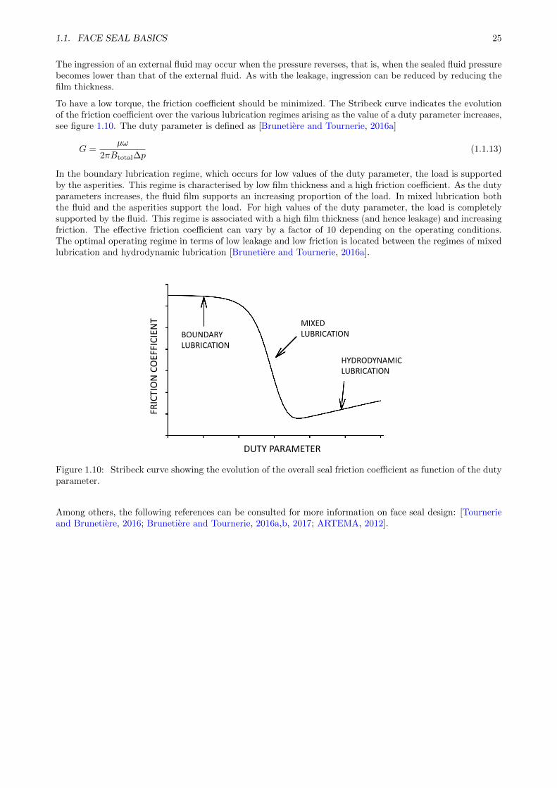
To have a low torque, the friction coefficient should be minimized. The Stribeck curve indicates the evolutionof the friction coefficient over the various lubrication regimes arising as the value of a duty parameter increases,see figure 1.10. The duty parameter is defined as [Brunetiere and Tournerie, 2016a]
G =µω
2πBtotal∆p(1.1.13)
In the boundary lubrication regime, which occurs for low values of the duty parameter, the load is supportedby the asperities. This regime is characterised by low film thickness and a high friction coefficient. As the dutyparameters increases, the fluid film supports an increasing proportion of the load. In mixed lubrication boththe fluid and the asperities support the load. For high values of the duty parameter, the load is completelysupported by the fluid. This regime is associated with a high film thickness (and hence leakage) and increasingfriction. The effective friction coefficient can vary by a factor of 10 depending on the operating conditions.The optimal operating regime in terms of low leakage and low friction is located between the regimes of mixedlubrication and hydrodynamic lubrication [Brunetiere and Tournerie, 2016a].
BOUNDARY LUBRICATION
MIXED LUBRICATION
HYDRODYNAMIC LUBRICATION
DUTY PARAMETER
FRIC
TIO
N C
OEF
FIC
IEN
T
Figure 1.10: Stribeck curve showing the evolution of the overall seal friction coefficient as function of the dutyparameter.
Among others, the following references can be consulted for more information on face seal design: [Tournerieand Brunetiere, 2016; Brunetiere and Tournerie, 2016a,b, 2017; ARTEMA, 2012].
26 CHAPTER 1. STATE OF THE ART
1.2 Review of face seals operating under severe transient conditions
This thesis is primarily interested in face seals operating in severe conditions. Such conditions are encounteredin various applications, including some types of pumps [Stekanko and Leishear, 2005; Leishear and Stekanko,2007], high power diesel engines [Fribourg et al., 2010], drilling tools [Throp et al., 2014; Burr, 2001; Wang et al.,2014], electrical submersible pumps used for oilfield production [Sarkis et al., 2013], heavy-duty boilers [Youngand Key, 2003], nuclear power plants [Mayer, 1989], aerospace turbopumps [NASA, 1978], desulphurization offlue gases [Schoepplein, 1986], etc.
More specifically, the demanding conditions of interest here are:
vibrations,
frequent and rapid starts of the system,
dynamic pressure variations and pressure inversions.
Mixed lubrication, contact, and surface defects can also detrimentally affect the behaviour of the face seal,and are reviewed as well.
1.2.1 Vibrations and misalignments
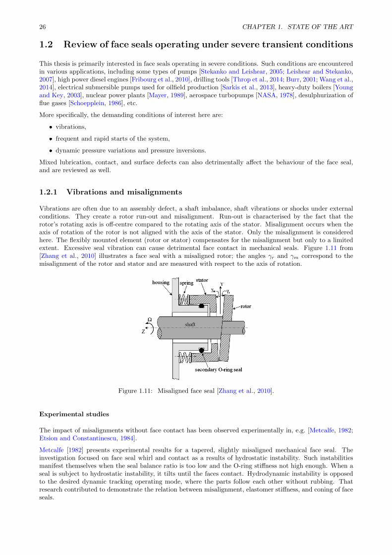
Vibrations are often due to an assembly defect, a shaft imbalance, shaft vibrations or shocks under externalconditions. They create a rotor run-out and misalignment. Run-out is characterised by the fact that therotor’s rotating axis is off-centre compared to the rotating axis of the stator. Misalignment occurs when theaxis of rotation of the rotor is not aligned with the axis of the stator. Only the misalignment is consideredhere. The flexibly mounted element (rotor or stator) compensates for the misalignment but only to a limitedextent. Excessive seal vibration can cause detrimental face contact in mechanical seals. Figure 1.11 from[Zhang et al., 2010] illustrates a face seal with a misaligned rotor; the angles γr and γm correspond to themisalignment of the rotor and stator and are measured with respect to the axis of rotation.
Figure 1.11: Misaligned face seal [Zhang et al., 2010].
Experimental studies
The impact of misalignments without face contact has been observed experimentally in, e.g. [Metcalfe, 1982;Etsion and Constantinescu, 1984].
Metcalfe [1982] presents experimental results for a tapered, slightly misaligned mechanical face seal. Theinvestigation focused on face seal whirl and contact as a results of hydrostatic instability. Such instabilitiesmanifest themselves when the seal balance ratio is too low and the O-ring stiffness not high enough. When aseal is subject to hydrostatic instability, it tilts until the faces contact. Hydrodynamic instability is opposedto the desired dynamic tracking operating mode, where the parts follow each other without rubbing. Thatresearch contributed to demonstrate the relation between misalignment, elastomer stiffness, and coning of faceseals.
1.2. REVIEW OF FACE SEALS OPERATING UNDER SEVERE TRANSIENT CONDITIONS 27
Etsion and Constantinescu [1984] present experimental results on a tapered, non-contacting face seal. Theresults show the variation of stator tilt and phase angle over time measured using proximity probes. Thesealing gap is also inferred based on leakage measurement. Two types of failure modes are observed. Forthe first failure mode, the stator tracks the rotor but the relative misalignment is so high that the faces arein contact. Wear marks are observed on both faces. The stator is evenly worn along the circumference. Incontrast, the rotor wear is manifested mostly at the rotor location which is the closest to the stator. Thesecond failure mode highlighted is a dynamic instability characterised by the stator’s inability to follow therotor.
Analytical studies
In parallel with the experimental observations, some authors have developed analytical models with the aimof providing estimates of the seals’ dynamic behavior.
Green and Etsion [1985] derived an analytical model predicting the dynamic behaviour of a non-contacting,tapered face seal. Three stability criteria were identified: (i) the faces must have a converging gap in thedirection of the flow, (ii) the rotational speed must be less than a threshold which depends on the inertiaand dynamic coefficients, and (iii) there is a limiting misalignment above which the faces may contact. Oneof the main equations is shown below. It allows estimating the relative transmissibility for given operatingconditions. The transmissibility is the ratio of relative misalignment γ0 due to rotor misalignment alone, tothe rotor misalignment γr(
γ0
γr
)2
=I2 +D2
s
(K − I)2 + (Ds + 0.5Dfluid)2(1.2.1)
Here, I is the support inertia coefficient, Ds the support damping coefficient, K the stiffness coefficient, andDfluid the fluid damping coefficient (all dimensionless). A good face tracking supposes a low value of γ0, whichis promoted by high values of the stiffness and damping coefficient. In contrast, high inertia leads to highrelative misalignment, which may lead to unstable behaviour. The limiting values of relative misalignmentare also provided in that article. The coefficients are derived from the dynamic film coefficients presented in[Green and Etsion, 1983] and based on earlier publications [Sharoni and Etsion, 1981; Etsion and Sharoni, 1980;Etsion, 1980]. These publications use small displacements to compute the forces, moments, and associatedstiffness and damping of narrow and aligned face seals. That research significantly contributed to the studyof misaligned face seals. The analytical model proposed enables immediate calculations for a misaligned faceseal.
That model has been largely used in subsequent work and extended to many types of face seal, in e.g. [Green,1987, 1990; Wileman and Green, 1991].
Numerical studies
Numerical models for misaligned face seals have also been proposed. They aim at estimating the overall faceseal performance while considering the effects of misalignment.
Etsion [1982] uses an analytical solution of the Reynolds equation along with a numerical solution of thenonlinear equations of motion for the face seal ring. The model is used to propose a seal stability map wherethree operating modes are identified: stable, unstable, and transition. In the stable mode, a disturbancedecreases over time, but in the unstable mode, it increases over time. In the transition mode, it remainsconstant over time. Groups of dimensionless parameters indicating transitions between the operating modesare identified. A study of the effect of various design parameters on the stability is also presented. Themain conclusions are that reducing the mass, radius of gyration, or operating speed; and increasing the springconstant, or the axial and angular stiffness encourage stable operation. The magnitude of the optimal valueof the coning angle for stable operation is also presented.
Tournerie and Frene [1984] or Green and Etsion [1986] developed a transient non-linear model to investigatethe effects of misalignment angle on the initial response of face seals. Such models solve the motion equationof the flexibly mounted element with the Reynolds equation over time.
28 CHAPTER 1. STATE OF THE ART
In [Tournerie and Frene, 1984], the equation of motion solved are Iχx1 = Mx,spring +Mx,fluid
Iχy1 = My,spring +My,fluid
mz = Fspring + Fhydraulic − Ffluid
(1.2.2)
with m the mass of the seal ring, I its moment of inertia (assumed equal in the different directions), whileM and F are the moments and forces applied by the fluid and support (only the spring is considered) to theflexibly-mounted element.
The equations are solved using time integration and a predictor-corrector method based on the Euler method.The contributions of the fluid are obtained from the pressure distribution solution of the Reynolds equation.The equation is solved using finite differences and a Gauss-Seidel iterative method with over-relaxation. Themodel is used for a parametric study covering a wide range of values of the misalignment angles for the stablecases. The stability observed is in accordance with the criteria of [Etsion, 1982].
Green and Etsion [1986] present a model solving the non-linear equation of motion for a flexibly mountedstator. The procedure starts by selecting arbitrary values for the amplitude γs, of the stator misalignmentamplitude, the phase angle φ, the axial displacement z and their derivative. The relative misalignment, γ, iscomputed using
γ =(γ2s + γ2
r − 2γsγr cos(φ− ωt))1/2
(1.2.3)
where γs and γr are, respectively, the stator and rotor misalignments, φ is the phase angle, and ω is therotational speed. The film thickness h is obtained using
h = C
(1 +
γ
1 + z/C0
r
r0cos θ +
β
1 + z/C0(r − riC0
)
)(1.2.4)
with β the coning angle, β = (h(ro) − h(ri))/(ro − ri), C the face centre distance, and C0 the designed facecentre distance. The pressure field and moments are calculated and the accelerations subsequently obtainedusing
γs =Mx
I+ φ2γs (1.2.5)
φ =
(My
I− 2φγs
)/γs (1.2.6)
1
C0z =
Fzm
(1.2.7)
with m, respectively, Fz, the dimensionless mass and axial force. The values are integrated with respect totime. The procedure is repeated until convergence. The model is used to evaluate the stability thresholdand steady state response of a flexibly mounted stator. A parametric study to explore the effect of variousdesign parameters and operating conditions is also presented. The main conclusions are that a high pressuredifference and optimal coning provide a high film stiffness, which reduces the risks of large misalignment andconsequently high leakage. Further, these numerical results were compared with the analytical predictions of[Green and Etsion, 1985]. A very good correlation was found for most cases and a fair correlation was foundfor the cases with more than small perturbations. Such results validate the use of the analytical model.
As highlighted above, the dynamic tracking mode is the desired and usual operating mode, in which theflexibly mounted part tracks the other. Some models have been developed specifically for such cases. Thecomputational time is significantly reduced, as no time integration technique is required since it is a stationaryconfiguration. The misalignment angles evolve as sine functions, and so do their derivatives. This approach isused in, e.g. [Person et al., 1997] or [Brunetiere et al., 2003a].
In [Person et al., 1997], the equations solved areMx,support +Mx,fluid − Iχx1 = 0
My,support +My,fluid − Iχy1 = 0Fz,support − Ffluid = 0
(1.2.8)
1.2. REVIEW OF FACE SEALS OPERATING UNDER SEVERE TRANSIENT CONDITIONS 29
with χx1 = χ1 cos(ωt + φ1) and χy1 = χ1 sin(ωt + φ1) the misalignment angles of the flexibly mounted stator.Equations 1.2.8 are solved using a Newton-Raphson method. The model is used to perform a parametricstudy evaluating the impact of varying operating conditions and grooves present on the faces. The mainobservations for the smooth face seal simulated are that the phase angle linearly decreases with increasingspeed, and increases and then decreases when the pressure difference is increased. Brunetiere et al. [2003a]use a similar method for the dynamic behaviour of the flexibly mounted element. This routine is coupled to afluid solver and a thermal solver. The authors show that the misalignment has only a limited impact on thetemperature distribution.
It is only recently that asperity contact has been considered in studies of misaligned face seals. Varney andGreen in [Varney and Green, 2016] present a numerical model for contacting face seals which includes a contactmodel, a solver for the non-linear equations of motion and an analytical expression for the film pressure. Themodel is used to simulate the behaviour of two contacting face seals. For the first case, the film thickness isshown to oscillate periodically at the rotating frequency and at half the rotating frequency; the minimum filmthickness is about four times the standard deviation of the surface roughness. In the second case, a heavycontact is imposed by considering flat surfaces. This leads to a rich non-linear response in the frequencydomain and repetitive face contact associated to system failure.
While all the models presented above cover a wide range of applications, none have the ability to predict theperformance of a non-narrow, contacting, misaligned face seal operating under varying conditions, such asthose encountered in severe environments.
Given that simulations of face seals in such conditions are targeted, the present model should include a generalmodel to capture the balance of the forces and moments of the flexibly mounted element.
1.2.2 Unsteady thermal effects
It is fundamental to consider thermal effects in face seals, since they determine the film temperature and hencethe viscosity and the temperature of the solids, and in turn the geometry of the seal faces. Thermal effectsare also responsible for some failure modes.
At rest, the two faces of the seal are usually pressed on each other to avoid leakage. As the shaft and rotorstart to rotate, a lift force is generated and the faces are taken apart, depending on the degree of contact ofthe seal. The heat generated deforms the seal rings, creating a coning of the seal faces and thus a non-uniformdistribution of the film thickness. This thermal coning brings about a hydrostatic load support and stabilityfor the inward face seals (leaking from outer to inner radius).
Issues associated with thermal effects
Rapid start ups induce strong thermal gradients. The sudden heat generated at the interface takes time todiffuse inside the seal parts. The face of the rotor and stator expand as a result of the heat but the back ofthe part is still cold and not expanded. This differential expansion leads to cracks originating at the rear ofthe part subject to extension [Kingery, 1953]. This heat checking failure mode due to transient thermal stressis also highlighted in [Nau, 1997]. Heat checking may also occur as a result of sudden cooling.
Another type of thermal cracking may occur when the face seal is suddenly put in contact with process fluidat a different temperature. Such a failure tends to be difficult to reproduce in the lab. Nyemeck et al. [2014]present a setup used to test face seals under a thermal shock of 100 K in 4 s. A face seal made of carbon andsilicon carbide was tested and showed no signs of damage.
Guichelaar et al. [2000] studied the blistering of carbon-graphite face seal faces which is a detrimental phe-nomenon associated to thermal effects. Blisters are noticeably burnished areas of elliptical or cylindrical shapeslightly elevated above the seal surface. Such face irregularities induce poor sealing performance and higherincidence of failure. Blistering occurs more readily with frequent starts and stops and higher rotational speeds.As part of that research, a test setup was designed to evaluate various grades of carbon-graphite seal materials.Blisters were characterised using interference microscopy and Raman spectroscopy. Based on the experimentalevidence, the authors concluded that the occurrence of blisters is not predictable and is not correlated withthe number of startup cycles.
Parmar [1992] presented a method to predict the susceptibility of a face seal to thermal cycling. Thermalcycling is a periodic variation of the face temperature, which can cause increased leakage, accelerated wear,and failure if it has a significant amplitude. Such effects were reported in, e.g. [Doust and Parmar, 1987;
30 CHAPTER 1. STATE OF THE ART
Salant et al., 1987; Rouillon, 2017]. The method proposed in the article is based on a two dimensional transientheat transfer model including thermal distortions, interface fluid load support, and contact. The numericalpredictions are validated with measurements. Based on the measurements, the thermal cycling mechanismappears to be possible if: there is significant thermal coning, there is a lag between the heat generation andthe thermal coning, and there is face contact. Further, the author found that increasing values of
√(α/k2),
where α is the diffusivity and k the thermal conductivity, are associated with a higher risk of thermal cycling.The general recommendations to reduce thermal cycling are: reduce thermal coning, reduce hard face contact,and choose a material pair with low contact friction.
Methods to capture thermal effects and deformations
Green [2002] developed a face seal model with an analytical contact model and 1D transient thermal deforma-tion model. The thermal model is based on the observation that the evolution of the thermal field is similarto a first order system response
tcharacdδ
dt+ δ = u(t) (1.2.9)
with δ = β/βref , β being the coning, with u(t) a unit step function, and tcharac a characteristic time. Thecharacteristic time tcharac and the steady state coning angle βref are obtained from off-line FEA. Using Laplacetransformations and step functions of the various types, constant, ramp-up, and ramp-down the above equationcan be solved analytically. The model is used to carry out a parametric study of the impact of the balanceratio and time constant on the performance of the face seal during start-up and shut-down. The start-up ismodelled as an increase of rotational speed and pressure, the shut-down as a decrease of rotational speed whilethe pressure is maintained. The author shows that the balance ratio has no significant effect on the transientresponse. However, this parameter strongly influences the leakage, as it controls the face centre distance. Also,when the time constant is increased, the deformation (coning) is delayed which leads to seal leakage for a shortperiod of time following shut-down.
The influence coefficient is a widely used method for capturing thermo-mechanical deformations [Xiong andSalant, 2002; Brunetiere et al., 2003a; Ruan et al., 1997; Harp and Salant, 1998]. With this method, thedeformation is assumed to be linearly related to the applied forces and rate of heat generation. The deformationat node ui follows a relation of the type
ui =
n∑j=1
(THijqj +MijFj) (1.2.10)
where the influence coefficients THij and Mij are the thermal and mechanical deformations at node i producedby a unit heat input and force at node j. qj is the generated heat flux at node j and Fj is the force due to thefluid and contact pressure at node j. The coefficients are computed off-line with an FEA method. This methodis time efficient when the boundary conditions are constant, as the influence coefficients are only computedonce. In transient cases or for varying boundary conditions, the influence coefficients have to be recomputed.Alternatively, Duhamel’s approximation method ([Ozisik, 1968]) can also be used, as in, e.g. [Salant and Bin,2005]. The thermal lag is found empirically from numerical experiments using a finite element thermal analysisof the seal. This semi-empirical approach was successfully used for simulating start-up and shut-down. Thismethod can be seen as the extension of the 1D method of [Green, 2002].
Another method is to embed a thermo-mechanical solver in the face seal numerical model. This approach isconvenient because there is no need for supplementary software, as the governing equations are directly solvedin the face seal model. A built-in mesher or a mesh-reader module has to be implemented in the code. If theboundary conditions do not change, there is no need to recompute the overall system. Such a method can beused to treat transient problems. The computation time is as good as with the influence coefficient methodThis method was applied in, e.g. [Migout et al., 2015].
Regarding the model developed in the present thesis, it is desirable to have an embedded thermo-mechanicalsolver to avoid relying on external software. Further, the code developed is based on previously existingmodules that include a built-in thermo-mechanical solver. For these reasons, it was decided to use a built-inthermo-mechanical solver to determine the temperature and deformations of the faces in the present model.
1.2. REVIEW OF FACE SEALS OPERATING UNDER SEVERE TRANSIENT CONDITIONS 31
Convective heat transfer
The convective heat transfer contributes significantly to the thermal behaviour and cooling of the face seal.The convective heat flux can be modelled as q(T ) = hc(T − Tref), with hc, in W/(K ·m), the convectioncoefficient, T the temperature of the wall, and Tref the known fluid temperature far from the wall. Here,hc is obtained from the Nusselt number Nu = hcD/kf , where D is the seal diameter and kf the thermalconductivity of the fluid. There are numerous publications proposing correlations for the Nusselt number onthe face seal [Becker, 1963; Ayadi et al., 2016; Luan and Khonsari, 2009b,a; Doane et al., 1991; Tachibanaet al., 1960; Childs and Long, 1996; Lebeck et al., 1998]. Overall, the Nusselt number is a power function ofthe Reynolds number ReD = ρωD/2µ and of the Prandtl number of the fluid Pr = Cpµ/kf , where Cp is theheat capacity of the fluid.
As an example, according to [Becker, 1963], for faces surrounded by a rotating fluid, the Nusselt number is
Nu = 0.133Re2/3D Pr1/3 (1.2.11)
This correlation was suggested for face seals by Lebeck [1991] and used in, e.g. [Brunetiere et al., 2003b;Nyemeck et al., 2015].
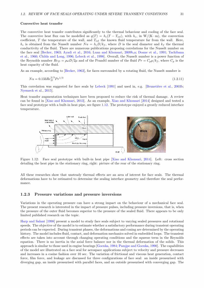
Heat transfer augmentation techniques have been proposed to reduce the risk of thermal damage. A reviewcan be found in [Xiao and Khonsari, 2013]. As an example, Xiao and Khonsari [2014] designed and tested aface seal prototype with a built-in heat pipe, see figure 1.12. The prototype enjoyed a greatly reduced interfacetemperature.
Figure 1.12: Face seal prototype with built-in heat pipe [Xiao and Khonsari, 2014]. Left: cross sectiondetailing the heat pipe in the stationary ring, right: picture of the rear of the stationary ring.
All these researches show that unsteady thermal effects are an area of interest for face seals. The thermaldeformations have to be estimated to determine the sealing interface geometry and therefore the seal perfor-mance.
1.2.3 Pressure variations and pressure inversions
Variations in the operating pressure can have a strong impact on the behaviour of a mechanical face seal.The present research is interested in the impact of pressure pulses, including pressure inversions, that is, whenthe pressure of the outer fluid becomes superior to the pressure of the sealed fluid. There appears to be onlylimited published research on the topic.
Harp and Salant [1998] present a model to study face seals subject to varying sealed pressures and rotationalspeeds. The objective of the model is to estimate whether a satisfactory performance during transient operatingperiods can be expected. During transient phases, the deformations and coning are determined by the operatinghistory. The model includes fluid, contact, and deformation mechanics solved in embedded loops. The transienteffects are taken into account through changing operating conditions and the squeeze term in the Reynoldsequation. There is no inertia in the axial force balance nor in the thermal deformation of the solids. Thisapproach is similar to those used in engine bearings [Goenka, 1984; Pamjpe and Goenka, 1990]. The capabilitiesof the model are illustrated on a face seal for aerospace applications subject to velocity and pressure decreasesand increases in a cosine fashion over 10 sec. The variation of frictional and viscous heat generation, contactforce, film force, and leakage are discussed for three configurations of face seal: an inside pressurised withdiverging gap, an inside pressurised with parallel faces, and an outside pressurised with converging gap. The
32 CHAPTER 1. STATE OF THE ART
first design suffers from excessively high contact pressures. The second has acceptable contact. The third hasalmost no contact pressure but a much greater leakage rate.
That study shows how some mechanisms impact the transient response of a face seal. The time scale of theunsteady processes are, however, of a few seconds and cannot be extended to smaller time scales. Further,there appears to be no work pertaining to face seals operating with pressure inversions.
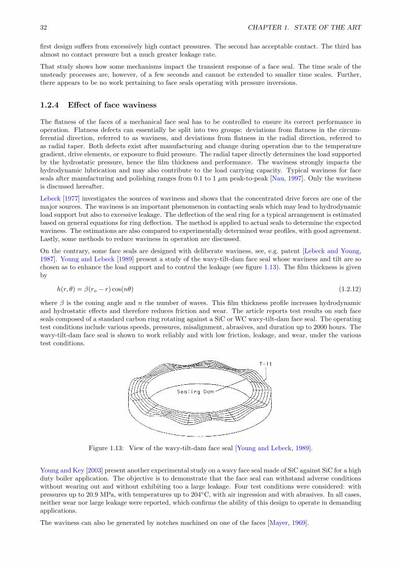
1.2.4 Effect of face waviness
The flatness of the faces of a mechanical face seal has to be controlled to ensure its correct performance inoperation. Flatness defects can essentially be split into two groups: deviations from flatness in the circum-ferential direction, referred to as waviness, and deviations from flatness in the radial direction, referred toas radial taper. Both defects exist after manufacturing and change during operation due to the temperaturegradient, drive elements, or exposure to fluid pressure. The radial taper directly determines the load supportedby the hydrostatic pressure, hence the film thickness and performance. The waviness strongly impacts thehydrodynamic lubrication and may also contribute to the load carrying capacity. Typical waviness for faceseals after manufacturing and polishing ranges from 0.1 to 1 µm peak-to-peak [Nau, 1997]. Only the wavinessis discussed hereafter.
Lebeck [1977] investigates the sources of waviness and shows that the concentrated drive forces are one of themajor sources. The waviness is an important phenomenon in contacting seals which may lead to hydrodynamicload support but also to excessive leakage. The deflection of the seal ring for a typical arrangement is estimatedbased on general equations for ring deflection. The method is applied to actual seals to determine the expectedwaviness. The estimations are also compared to experimentally determined wear profiles, with good agreement.Lastly, some methods to reduce waviness in operation are discussed.
On the contrary, some face seals are designed with deliberate waviness, see, e.g. patent [Lebeck and Young,1987]. Young and Lebeck [1989] present a study of the wavy-tilt-dam face seal whose waviness and tilt are sochosen as to enhance the load support and to control the leakage (see figure 1.13). The film thickness is givenby
h(r, θ) = β(ro − r) cos(nθ) (1.2.12)
where β is the coning angle and n the number of waves. This film thickness profile increases hydrodynamicand hydrostatic effects and therefore reduces friction and wear. The article reports test results on such faceseals composed of a standard carbon ring rotating against a SiC or WC wavy-tilt-dam face seal. The operatingtest conditions include various speeds, pressures, misalignment, abrasives, and duration up to 2000 hours. Thewavy-tilt-dam face seal is shown to work reliably and with low friction, leakage, and wear, under the varioustest conditions.
Figure 1.13: View of the wavy-tilt-dam face seal [Young and Lebeck, 1989].
Young and Key [2003] present another experimental study on a wavy face seal made of SiC against SiC for a highduty boiler application. The objective is to demonstrate that the face seal can withstand adverse conditionswithout wearing out and without exhibiting too a large leakage. Four test conditions were considered: withpressures up to 20.9 MPa, with temperatures up to 204C, with air ingression and with abrasives. In all cases,neither wear nor large leakage were reported, which confirms the ability of this design to operate in demandingapplications.
The waviness can also be generated by notches machined on one of the faces [Mayer, 1969].
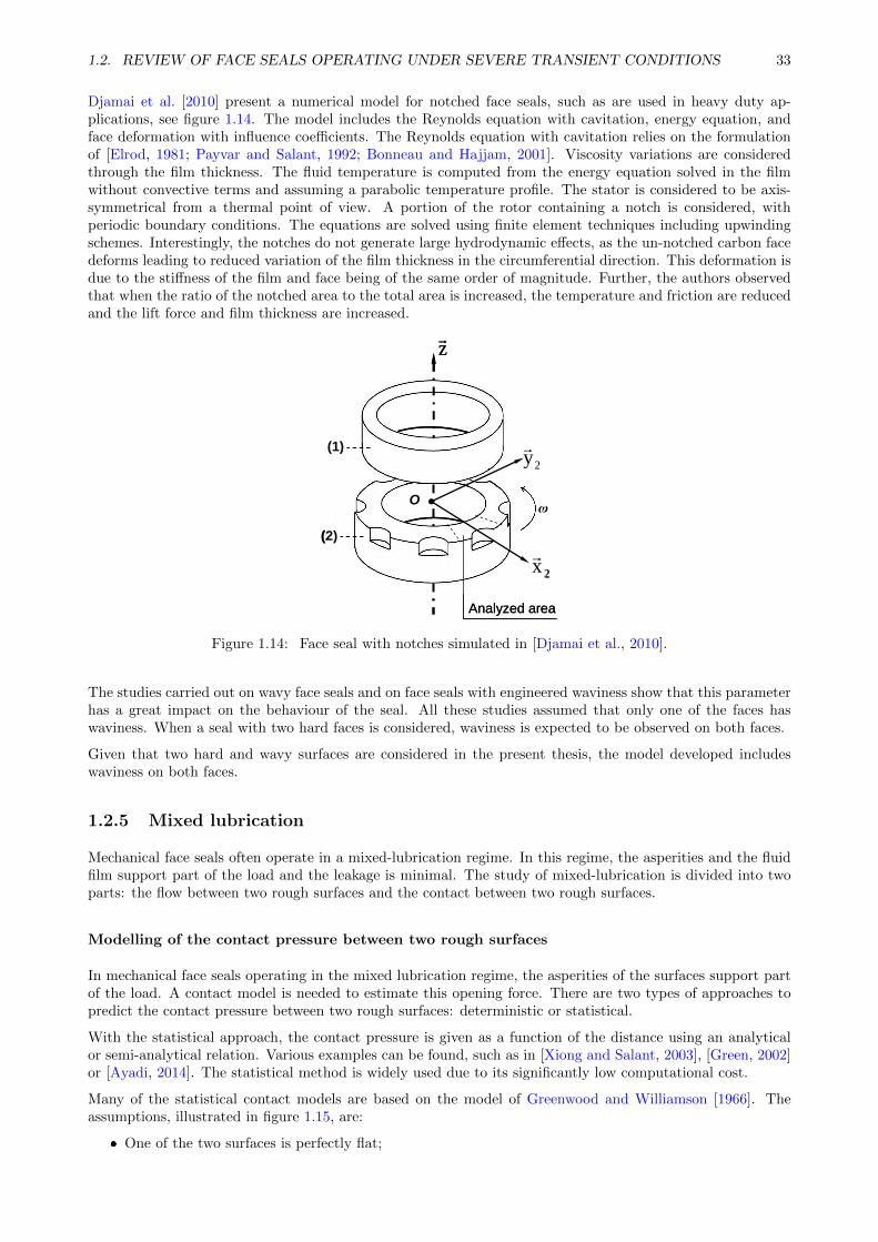
1.2. REVIEW OF FACE SEALS OPERATING UNDER SEVERE TRANSIENT CONDITIONS 33
Djamai et al. [2010] present a numerical model for notched face seals, such as are used in heavy duty ap-plications, see figure 1.14. The model includes the Reynolds equation with cavitation, energy equation, andface deformation with influence coefficients. The Reynolds equation with cavitation relies on the formulationof [Elrod, 1981; Payvar and Salant, 1992; Bonneau and Hajjam, 2001]. Viscosity variations are consideredthrough the film thickness. The fluid temperature is computed from the energy equation solved in the filmwithout convective terms and assuming a parabolic temperature profile. The stator is considered to be axis-symmetrical from a thermal point of view. A portion of the rotor containing a notch is considered, withperiodic boundary conditions. The equations are solved using finite element techniques including upwindingschemes. Interestingly, the notches do not generate large hydrodynamic effects, as the un-notched carbon facedeforms leading to reduced variation of the film thickness in the circumferential direction. This deformation isdue to the stiffness of the film and face being of the same order of magnitude. Further, the authors observedthat when the ratio of the notched area to the total area is increased, the temperature and friction are reducedand the lift force and film thickness are increased.
O
(1)
(2)
ω
z
2y
2x
Analyzed area
O
(1)
(2)
ω
z
2y
2x
Analyzed area
Figure 1.14: Face seal with notches simulated in [Djamai et al., 2010].
The studies carried out on wavy face seals and on face seals with engineered waviness show that this parameterhas a great impact on the behaviour of the seal. All these studies assumed that only one of the faces haswaviness. When a seal with two hard faces is considered, waviness is expected to be observed on both faces.
Given that two hard and wavy surfaces are considered in the present thesis, the model developed includeswaviness on both faces.
1.2.5 Mixed lubrication
Mechanical face seals often operate in a mixed-lubrication regime. In this regime, the asperities and the fluidfilm support part of the load and the leakage is minimal. The study of mixed-lubrication is divided into twoparts: the flow between two rough surfaces and the contact between two rough surfaces.
Modelling of the contact pressure between two rough surfaces
In mechanical face seals operating in the mixed lubrication regime, the asperities of the surfaces support partof the load. A contact model is needed to estimate this opening force. There are two types of approaches topredict the contact pressure between two rough surfaces: deterministic or statistical.
With the statistical approach, the contact pressure is given as a function of the distance using an analyticalor semi-analytical relation. Various examples can be found, such as in [Xiong and Salant, 2003], [Green, 2002]or [Ayadi, 2014]. The statistical method is widely used due to its significantly low computational cost.
Many of the statistical contact models are based on the model of Greenwood and Williamson [1966]. Theassumptions, illustrated in figure 1.15, are:
One of the two surfaces is perfectly flat;
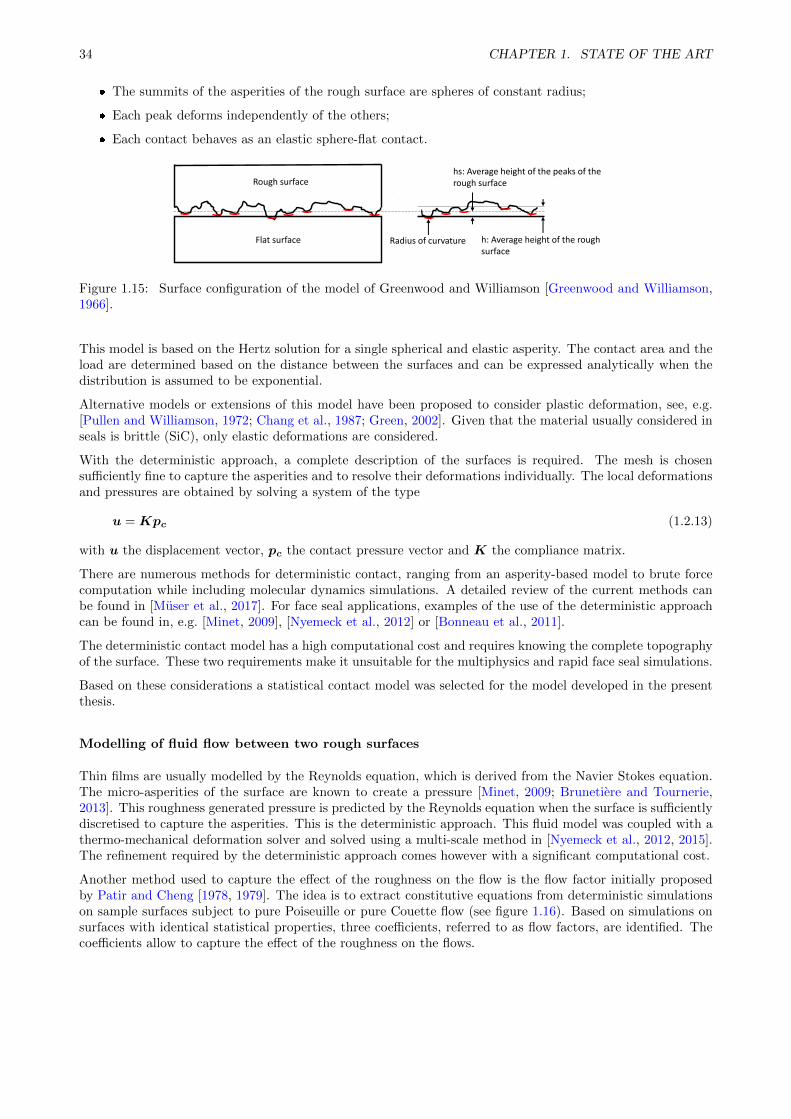
34 CHAPTER 1. STATE OF THE ART
The summits of the asperities of the rough surface are spheres of constant radius;
Each peak deforms independently of the others;
Each contact behaves as an elastic sphere-flat contact.
Flat surface h: Average height of the rough surface
hs: Average height of the peaks of the rough surface Rough surface
Radius of curvature
Figure 1.15: Surface configuration of the model of Greenwood and Williamson [Greenwood and Williamson,1966].
This model is based on the Hertz solution for a single spherical and elastic asperity. The contact area and theload are determined based on the distance between the surfaces and can be expressed analytically when thedistribution is assumed to be exponential.
Alternative models or extensions of this model have been proposed to consider plastic deformation, see, e.g.[Pullen and Williamson, 1972; Chang et al., 1987; Green, 2002]. Given that the material usually considered inseals is brittle (SiC), only elastic deformations are considered.
With the deterministic approach, a complete description of the surfaces is required. The mesh is chosensufficiently fine to capture the asperities and to resolve their deformations individually. The local deformationsand pressures are obtained by solving a system of the type
u = Kpc (1.2.13)
with u the displacement vector, pc the contact pressure vector and K the compliance matrix.
There are numerous methods for deterministic contact, ranging from an asperity-based model to brute forcecomputation while including molecular dynamics simulations. A detailed review of the current methods canbe found in [Muser et al., 2017]. For face seal applications, examples of the use of the deterministic approachcan be found in, e.g. [Minet, 2009], [Nyemeck et al., 2012] or [Bonneau et al., 2011].
The deterministic contact model has a high computational cost and requires knowing the complete topographyof the surface. These two requirements make it unsuitable for the multiphysics and rapid face seal simulations.
Based on these considerations a statistical contact model was selected for the model developed in the presentthesis.
Modelling of fluid flow between two rough surfaces
Thin films are usually modelled by the Reynolds equation, which is derived from the Navier Stokes equation.The micro-asperities of the surface are known to create a pressure [Minet, 2009; Brunetiere and Tournerie,2013]. This roughness generated pressure is predicted by the Reynolds equation when the surface is sufficientlydiscretised to capture the asperities. This is the deterministic approach. This fluid model was coupled with athermo-mechanical deformation solver and solved using a multi-scale method in [Nyemeck et al., 2012, 2015].The refinement required by the deterministic approach comes however with a significant computational cost.
Another method used to capture the effect of the roughness on the flow is the flow factor initially proposedby Patir and Cheng [1978, 1979]. The idea is to extract constitutive equations from deterministic simulationson sample surfaces subject to pure Poiseuille or pure Couette flow (see figure 1.16). Based on simulations onsurfaces with identical statistical properties, three coefficients, referred to as flow factors, are identified. Thecoefficients allow to capture the effect of the roughness on the flows.
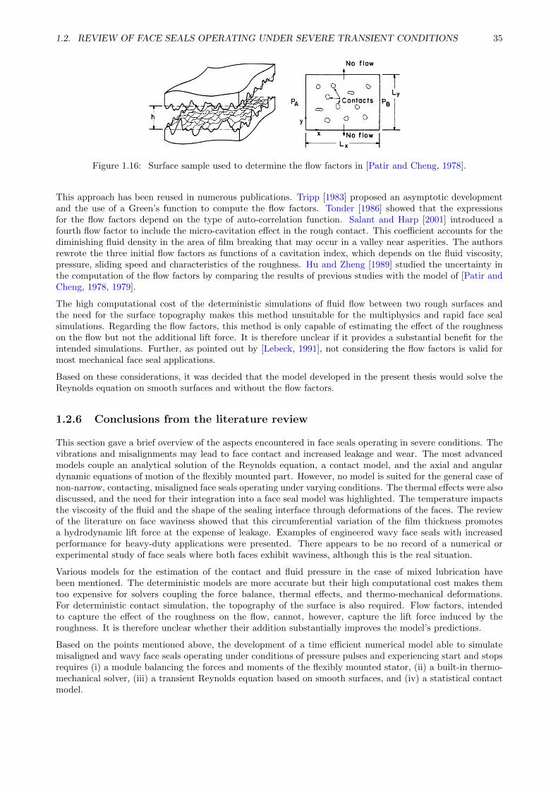
1.2. REVIEW OF FACE SEALS OPERATING UNDER SEVERE TRANSIENT CONDITIONS 35
Figure 1.16: Surface sample used to determine the flow factors in [Patir and Cheng, 1978].
This approach has been reused in numerous publications. Tripp [1983] proposed an asymptotic developmentand the use of a Green’s function to compute the flow factors. Tonder [1986] showed that the expressionsfor the flow factors depend on the type of auto-correlation function. Salant and Harp [2001] introduced afourth flow factor to include the micro-cavitation effect in the rough contact. This coefficient accounts for thediminishing fluid density in the area of film breaking that may occur in a valley near asperities. The authorsrewrote the three initial flow factors as functions of a cavitation index, which depends on the fluid viscosity,pressure, sliding speed and characteristics of the roughness. Hu and Zheng [1989] studied the uncertainty inthe computation of the flow factors by comparing the results of previous studies with the model of [Patir andCheng, 1978, 1979].
The high computational cost of the deterministic simulations of fluid flow between two rough surfaces andthe need for the surface topography makes this method unsuitable for the multiphysics and rapid face sealsimulations. Regarding the flow factors, this method is only capable of estimating the effect of the roughnesson the flow but not the additional lift force. It is therefore unclear if it provides a substantial benefit for theintended simulations. Further, as pointed out by [Lebeck, 1991], not considering the flow factors is valid formost mechanical face seal applications.
Based on these considerations, it was decided that the model developed in the present thesis would solve theReynolds equation on smooth surfaces and without the flow factors.
1.2.6 Conclusions from the literature review
This section gave a brief overview of the aspects encountered in face seals operating in severe conditions. Thevibrations and misalignments may lead to face contact and increased leakage and wear. The most advancedmodels couple an analytical solution of the Reynolds equation, a contact model, and the axial and angulardynamic equations of motion of the flexibly mounted part. However, no model is suited for the general case ofnon-narrow, contacting, misaligned face seals operating under varying conditions. The thermal effects were alsodiscussed, and the need for their integration into a face seal model was highlighted. The temperature impactsthe viscosity of the fluid and the shape of the sealing interface through deformations of the faces. The reviewof the literature on face waviness showed that this circumferential variation of the film thickness promotesa hydrodynamic lift force at the expense of leakage. Examples of engineered wavy face seals with increasedperformance for heavy-duty applications were presented. There appears to be no record of a numerical orexperimental study of face seals where both faces exhibit waviness, although this is the real situation.
Various models for the estimation of the contact and fluid pressure in the case of mixed lubrication havebeen mentioned. The deterministic models are more accurate but their high computational cost makes themtoo expensive for solvers coupling the force balance, thermal effects, and thermo-mechanical deformations.For deterministic contact simulation, the topography of the surface is also required. Flow factors, intendedto capture the effect of the roughness on the flow, cannot, however, capture the lift force induced by theroughness. It is therefore unclear whether their addition substantially improves the model’s predictions.
Based on the points mentioned above, the development of a time efficient numerical model able to simulatemisaligned and wavy face seals operating under conditions of pressure pulses and experiencing start and stopsrequires (i) a module balancing the forces and moments of the flexibly mounted stator, (ii) a built-in thermo-mechanical solver, (iii) a transient Reynolds equation based on smooth surfaces, and (iv) a statistical contactmodel.

36 CHAPTER 1. STATE OF THE ART
1.3 Summary of the state of the art
This section has presented some elementary considerations regarding face seals, in particular:
The main components and operating principles;
The design specifications and general design rules;
Elementary equations used to obtain a first idea of the expected performance.
Further, a review of the current research pertaining to face seals operating in severe conditions was presentedto position the current research work. It covered:
Experimental, analytical and numerical research on vibrations and misalignments;
Thermal effects in face seals, the associated issues and methods to include them in models;
The effect of face waviness;
Methods used to capture mixed-lubrication, which include modelling of the pressure generated by micro-asperities of the surface and contact pressure.
Chapter 2
Face seal modelling
The objective of this chapter is to present the equations governing the behaviour of the face seal and the nu-merical techniques employed for their solution. The resulting code will be verified by comparing its predictionsto published results and validated with experimental data in chapter 3 of the thesis. The verified and validatedcode will be used for the numerical and experimental studies in chapter 5.
Contents2.1 Modelling strategy and model building . . . . . . . . . . . . . . . . . . . . . . . . 37
2.2 The continuous equations . . . . . . . . . . . . . . . . . . . . . . . . . . . . . . . . 39
2.2.1 Face kinematic description . . . . . . . . . . . . . . . . . . . . . . . . . . . . . . . . . 39
2.2.2 Axial and angular balance of a flexibly mounted stator . . . . . . . . . . . . . . . . . 42
2.2.3 Reynolds equation . . . . . . . . . . . . . . . . . . . . . . . . . . . . . . . . . . . . . 45
2.2.4 Contact model . . . . . . . . . . . . . . . . . . . . . . . . . . . . . . . . . . . . . . . 48
2.2.5 Energy equations and thermo-mechanical deformation equations . . . . . . . . . . . 49
2.2.6 Coupling strategies . . . . . . . . . . . . . . . . . . . . . . . . . . . . . . . . . . . . . 51
2.2.7 Closing remarks . . . . . . . . . . . . . . . . . . . . . . . . . . . . . . . . . . . . . . 52
2.3 Discrete equations . . . . . . . . . . . . . . . . . . . . . . . . . . . . . . . . . . . . . 53
2.3.1 Spatial discretisation using the finite element method . . . . . . . . . . . . . . . . . 53
2.3.2 Time integration schemes . . . . . . . . . . . . . . . . . . . . . . . . . . . . . . . . . 58
2.4 Numerical algorithms . . . . . . . . . . . . . . . . . . . . . . . . . . . . . . . . . . . 63
2.4.1 Non-linear algorithm for the Reynolds equation . . . . . . . . . . . . . . . . . . . . . 63
2.4.2 Non-linear algorithm for the axial and angular force balance solver . . . . . . . . . . 65
2.4.3 Closing remarks . . . . . . . . . . . . . . . . . . . . . . . . . . . . . . . . . . . . . . 67
2.4.4 Code workflow . . . . . . . . . . . . . . . . . . . . . . . . . . . . . . . . . . . . . . . 68
2.5 Summary of the face seal modelling strategy . . . . . . . . . . . . . . . . . . . . . 70
2.1 Modelling strategy and model building
The general process of going from the physical phenomena governing the behaviour of a system to a numericalsolver capable of predicting the performance of the system is shown in figure 2.1. The phenomena governing thebehaviour of face seals dictate the equations to be considered for building the model. Based on these generalequations, closures and assumptions are selected to derive specific governing equations. The specific equationsare discretised in space and time and formulated in an algorithmic manner to construct the numerical solver.
37
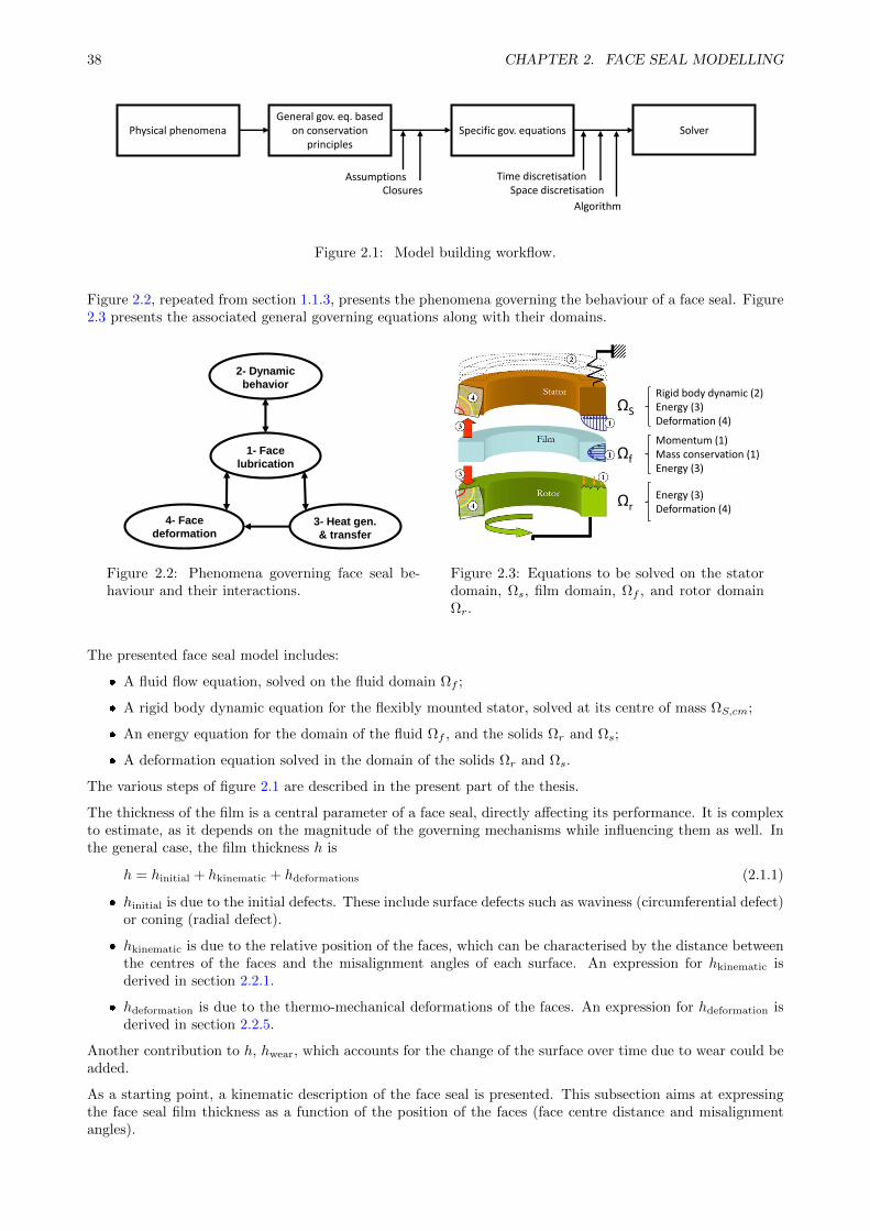
38 CHAPTER 2. FACE SEAL MODELLING
Physical phenomenaGeneral gov. eq. based
on conservation principles
AssumptionsClosures
Specific gov. equations Solver
Space discretisationTime discretisation
Algorithm
Figure 2.1: Model building workflow.
Figure 2.2, repeated from section 1.1.3, presents the phenomena governing the behaviour of a face seal. Figure2.3 presents the associated general governing equations along with their domains.
1- Face
lubrication
2- Dynamic
behavior
3- Heat gen.
& transfer
4- Face
deformation
Figure 2.2: Phenomena governing face seal be-haviour and their interactions.
Momentum (1)Mass conservation (1)Energy (3)
Rigid body dynamic (2)Energy (3)Deformation (4)
Energy (3)Deformation (4)
ΩS
Ωf
Ωr
Figure 2.3: Equations to be solved on the statordomain, Ωs, film domain, Ωf , and rotor domainΩr.
The presented face seal model includes:
A fluid flow equation, solved on the fluid domain Ωf ;
A rigid body dynamic equation for the flexibly mounted stator, solved at its centre of mass ΩS,cm;
An energy equation for the domain of the fluid Ωf , and the solids Ωr and Ωs;
A deformation equation solved in the domain of the solids Ωr and Ωs.
The various steps of figure 2.1 are described in the present part of the thesis.
The thickness of the film is a central parameter of a face seal, directly affecting its performance. It is complexto estimate, as it depends on the magnitude of the governing mechanisms while influencing them as well. Inthe general case, the film thickness h is
h = hinitial + hkinematic + hdeformations (2.1.1)
hinitial is due to the initial defects. These include surface defects such as waviness (circumferential defect)or coning (radial defect).
hkinematic is due to the relative position of the faces, which can be characterised by the distance betweenthe centres of the faces and the misalignment angles of each surface. An expression for hkinematic isderived in section 2.2.1.
hdeformation is due to the thermo-mechanical deformations of the faces. An expression for hdeformation isderived in section 2.2.5.
Another contribution to h, hwear, which accounts for the change of the surface over time due to wear could beadded.
As a starting point, a kinematic description of the face seal is presented. This subsection aims at expressingthe face seal film thickness as a function of the position of the faces (face centre distance and misalignmentangles).
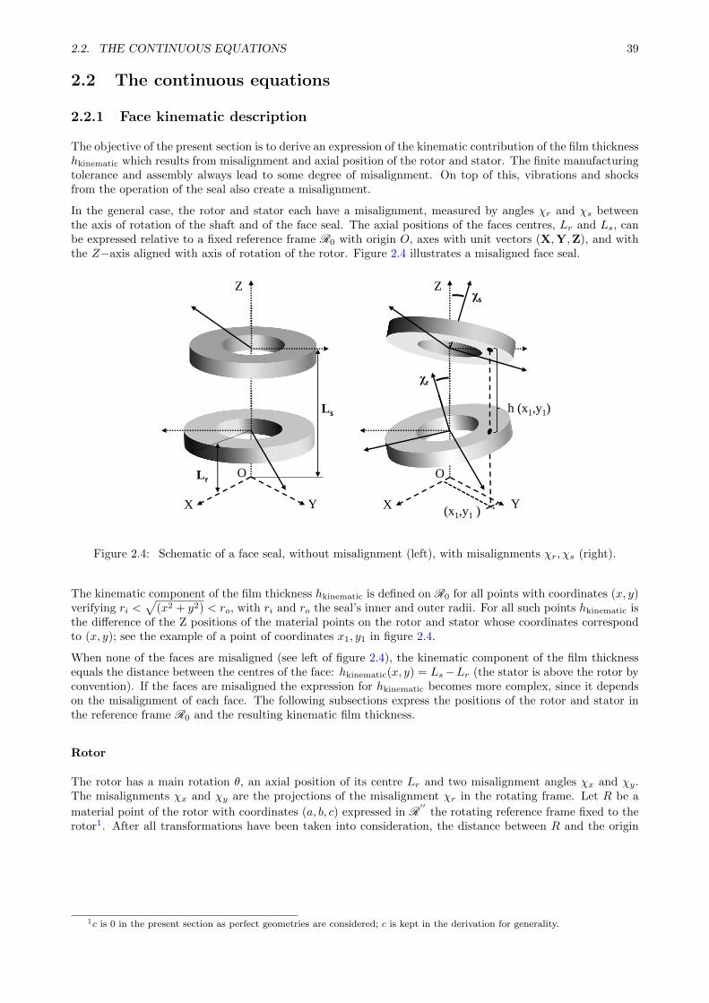
2.2. THE CONTINUOUS EQUATIONS 39
2.2 The continuous equations
2.2.1 Face kinematic description
The objective of the present section is to derive an expression of the kinematic contribution of the film thicknesshkinematic which results from misalignment and axial position of the rotor and stator. The finite manufacturingtolerance and assembly always lead to some degree of misalignment. On top of this, vibrations and shocksfrom the operation of the seal also create a misalignment.
In the general case, the rotor and stator each have a misalignment, measured by angles χr and χs betweenthe axis of rotation of the shaft and of the face seal. The axial positions of the faces centres, Lr and Ls, canbe expressed relative to a fixed reference frame R0 with origin O, axes with unit vectors (X,Y,Z), and withthe Z−axis aligned with axis of rotation of the rotor. Figure 2.4 illustrates a misaligned face seal.
χr
χs
XY
Z
Y
Z
X
h (x1,y1)
(x1,y1 )
OLr
Ls
O
Figure 2.4: Schematic of a face seal, without misalignment (left), with misalignments χr, χs (right).
The kinematic component of the film thickness hkinematic is defined on R0 for all points with coordinates (x, y)verifying ri <
√(x2 + y2) < ro, with ri and ro the seal’s inner and outer radii. For all such points hkinematic is
the difference of the Z positions of the material points on the rotor and stator whose coordinates correspondto (x, y); see the example of a point of coordinates x1, y1 in figure 2.4.
When none of the faces are misaligned (see left of figure 2.4), the kinematic component of the film thicknessequals the distance between the centres of the face: hkinematic(x, y) = Ls−Lr (the stator is above the rotor byconvention). If the faces are misaligned the expression for hkinematic becomes more complex, since it dependson the misalignment of each face. The following subsections express the positions of the rotor and stator inthe reference frame R0 and the resulting kinematic film thickness.
Rotor
The rotor has a main rotation θ, an axial position of its centre Lr and two misalignment angles χx and χy.The misalignments χx and χy are the projections of the misalignment χr in the rotating frame. Let R be a
material point of the rotor with coordinates (a, b, c) expressed in R′′
the rotating reference frame fixed to therotor1. After all transformations have been taken into consideration, the distance between R and the origin
1c is 0 in the present section as perfect geometries are considered; c is kept in the derivation for generality.
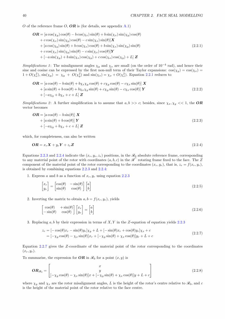
40 CHAPTER 2. FACE SEAL MODELLING
O of the reference frame O, OR is (for details, see appendix A.1)
OR = [a cos(χy) cos(θ)− b cos(χx) sin(θ) + b sin(χx) sin(χy) cos(θ)
+ c cos(χx) sin(χy) cos(θ)− c sin(χx) sin(θ)]X
+ [a cos(χy) sin(θ) + b cos(χx) cos(θ) + b sin(χx) sin(χy) sin(θ)
+ c cos(χx) sin(χy) sin(θ)− c sin(χx) cos(θ)]Y
+ [−a sin(χy) + b sin(χx) cos(χy) + c cos(χx) cos(χy) + L] Z
(2.2.1)
Simplifications 1 : The misalignment angles χy and χx are small (on the order of 10−4 rad), and hence theirsine and cosine can be expressed by the first non-null term of their Taylor expansions: cos(χy) = cos(χx) =1 +O(χ2
x), sin(χy) = χy + O(χ2y) and sin(χx) = χx +O(χ2
x). Equation 2.2.1 reduces to
OR = [a cos(θ)− b sin(θ) + bχxχy cos(θ) + cχy cos(θ)− cχx sin(θ)] X
+ [a sin(θ) + b cos(θ) + bχxχy sin(θ) + cχy sin(θ)− cχx cos(θ)] Y
+ [−aχy + bχx + c+ L] Z
(2.2.2)
Simplifications 2 : A further simplification is to assume that a, b >> c; besides, since χx, χy << 1, the ORvector becomes
OR = [a cos(θ)− b sin(θ)] X
+ [a sin(θ) + b cos(θ)] Y
+ [−aχy + bχx + c+ L] Z
(2.2.3)
which, for completeness, can also be written
OR = xrX + yrY + zrZ (2.2.4)
Equations 2.2.3 and 2.2.4 indicate the (xr, yr, zr) positions, in the R0 absolute reference frame, correspondingto any material point of the rotor with coordinates (a, b, c) in the R
′′rotating frame fixed to the face. The Z
component of the material point of the rotor corresponding to the coordinates (xr, yr), that is, zr = f(xr, yr),is obtained by combining equations 2.2.3 and 2.2.4:
1. Express a and b as a function of xr, yr using equation 2.2.3[xryr
]=
[cos(θ) − sin(θ)sin(θ) cos(θ)
] [ab
](2.2.5)
2. Inverting the matrix to obtain a, b = f(xr, yr), yields[cos(θ) + sin(θ)− sin(θ) cos(θ)
] [xryr
]=
[ab
](2.2.6)
3. Replacing a, b by their expression in terms of X,Y in the Z-equation of equation yields 2.2.3
zr = [− cos(θ)xr − sin(θ)yr]χy + L+ [− sin(θ)xr + cos(θ)yr]χx + c
= [−χy cos(θ)− χx sin(θ)]xr + [−χy sin(θ) + χx cos(θ)]yr + L+ c(2.2.7)
Equation 2.2.7 gives the Z-coordinate of the material point of the rotor corresponding to the coordinates(xr, yr).
To summarise, the expression for OR in R0 for a point (x, y) is
ORR0 =
xy
[−χy cos(θ)− χx sin(θ)]x+ [−χy sin(θ) + χx cos(θ)]y + L+ c
(2.2.8)
where χy and χx are the rotor misalignment angles, L is the height of the rotor’s centre relative to R0, and cis the height of the material point of the rotor relative to the face centre.
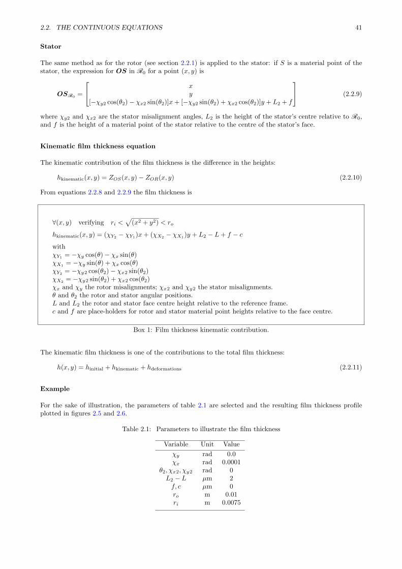
2.2. THE CONTINUOUS EQUATIONS 41
Stator
The same method as for the rotor (see section 2.2.1) is applied to the stator: if S is a material point of thestator, the expression for OS in R0 for a point (x, y) is
OSR0=
xy
[−χy2 cos(θ2)− χx2 sin(θ2)]x+ [−χy2 sin(θ2) + χx2 cos(θ2)]y + L2 + f
(2.2.9)
where χy2 and χx2 are the stator misalignment angles, L2 is the height of the stator’s centre relative to R0,and f is the height of a material point of the stator relative to the centre of the stator’s face.
Kinematic film thickness equation
The kinematic contribution of the film thickness is the difference in the heights:
hkinematic(x, y) = ZOS(x, y)− ZOR(x, y) (2.2.10)
From equations 2.2.8 and 2.2.9 the film thickness is
∀(x, y) verifying ri <√
(x2 + y2) < ro
hkinematic(x, y) = (χY2 − χY1)x+ (χX2 − χX1)y + L2 − L+ f − cwithχY1 = −χy cos(θ)− χx sin(θ)χX1
= −χy sin(θ) + χx cos(θ)χY2
= −χy2 cos(θ2)− χx2 sin(θ2)χX2
= −χy2 sin(θ2) + χx2 cos(θ2)χx and χy the rotor misalignments; χx2 and χy2 the stator misalignments.θ and θ2 the rotor and stator angular positions.L and L2 the rotor and stator face centre height relative to the reference frame.c and f are place-holders for rotor and stator material point heights relative to the face centre.
Box 1: Film thickness kinematic contribution.
The kinematic film thickness is one of the contributions to the total film thickness:
h(x, y) = hinitial + hkinematic + hdeformations (2.2.11)
Example
For the sake of illustration, the parameters of table 2.1 are selected and the resulting film thickness profileplotted in figures 2.5 and 2.6.
Table 2.1: Parameters to illustrate the film thickness
Variable Unit Value
χy rad 0.0χx rad 0.0001
θ2, χx2, χy2 rad 0L2 − L µm 2f, c µm 0ro m 0.01ri m 0.0075
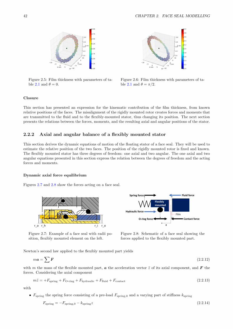
42 CHAPTER 2. FACE SEAL MODELLING
X mm
105
05
10
Y mm
10
5
0
5
10
Z um
1.0
1.5
2.0
2.5
3.0
1.00
1.25
1.50
1.75
2.00
2.25
2.50
2.75
3.00
Figure 2.5: Film thickness with parameters of ta-ble 2.1 and θ = 0.
X mm
105
05
10
Y mm
10
5
0
5
10
Z um
1.0
1.5
2.0
2.5
3.0
1.0
1.2
1.4
1.6
1.8
2.0
2.2
2.4
2.6
2.8
3.0
Figure 2.6: Film thickness with parameters of ta-ble 2.1 and θ = π/2.
Closure
This section has presented an expression for the kinematic contribution of the film thickness, from knownrelative positions of the faces. The misalignment of the rigidly mounted rotor creates forces and moments thatare transmitted to the fluid and to the flexibly-mounted stator, thus changing its position. The next sectionpresents the relations between the forces, moments, and the resulting axial and angular positions of the stator.
2.2.2 Axial and angular balance of a flexibly mounted stator
This section derives the dynamic equations of motion of the floating stator of a face seal. They will be used toestimate the relative position of the two faces. The position of the rigidly mounted rotor is fixed and known.The flexibly mounted stator has three degrees of freedom: one axial and two angular. The one axial and twoangular equations presented in this section express the relation between the degrees of freedom and the actingforces and moments.
Dynamic axial force equilibrium
Figures 2.7 and 2.8 show the forces acting on a face seal.
r_o r_h r_i r_o
Figure 2.7: Example of a face seal with radii po-sition, flexibly mounted element on the left.
Flexibly mounted
Film
Fluid force
Contact forceO-ring force
Spring force
Hydraulic force
z
Figure 2.8: Schematic of a face seal showing theforces applied to the flexibly mounted part.
Newton’s second law applied to the flexibly mounted part yields
ma =∑
F (2.2.12)
with m the mass of the flexible mounted part, a the acceleration vector z of its axial component, and F theforces. Considering the axial component
mz = +Fspring + FO-ring + Fhydraulic + Ffluid + Fcontact (2.2.13)
with
Fspring the spring force consisting of a pre-load Fspring,0 and a varying part of stiffness kspring
Fspring = −Fspring,0 − kspringz (2.2.14)
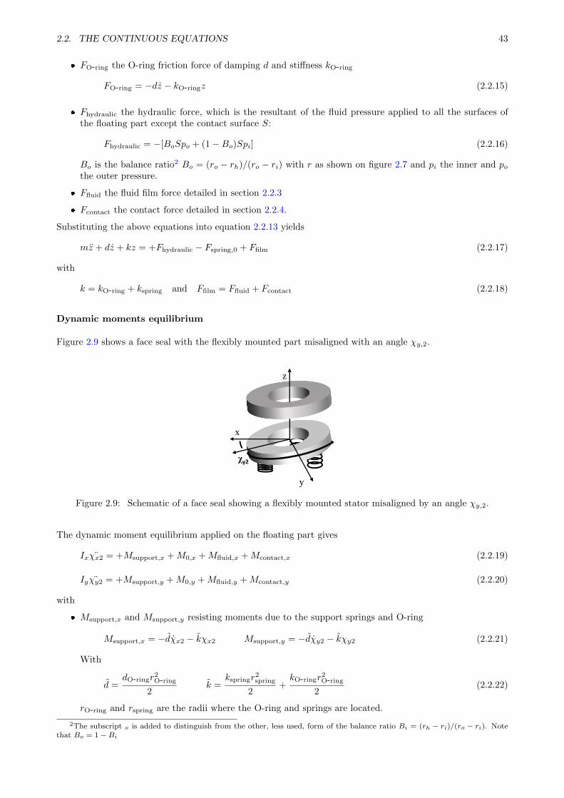
2.2. THE CONTINUOUS EQUATIONS 43
FO-ring the O-ring friction force of damping d and stiffness kO-ring
FO-ring = −dz − kO-ringz (2.2.15)
Fhydraulic the hydraulic force, which is the resultant of the fluid pressure applied to all the surfaces ofthe floating part except the contact surface S:
Fhydraulic = −[BoSpo + (1−Bo)Spi] (2.2.16)
Bo is the balance ratio2 Bo = (ro − rh)/(ro − ri) with r as shown on figure 2.7 and pi the inner and pothe outer pressure.
Ffluid the fluid film force detailed in section 2.2.3
Fcontact the contact force detailed in section 2.2.4.
Substituting the above equations into equation 2.2.13 yields
mz + dz + kz = +Fhydraulic − Fspring,0 + Ffilm (2.2.17)
with
k = kO-ring + kspring and Ffilm = Ffluid + Fcontact (2.2.18)
Dynamic moments equilibrium
Figure 2.9 shows a face seal with the flexibly mounted part misaligned with an angle χy,2.
χy2
y
x
z
Figure 2.9: Schematic of a face seal showing a flexibly mounted stator misaligned by an angle χy,2.
The dynamic moment equilibrium applied on the floating part gives
Ixχx2 = +Msupport,x +M0,x +Mfluid,x +Mcontact,x (2.2.19)
Iyχy2 = +Msupport,y +M0,y +Mfluid,y +Mcontact,y (2.2.20)
with
Msupport,x and Msupport,y resisting moments due to the support springs and O-ring
Msupport,x = −dχx2 − kχx2 Msupport,y = −dχy2 − kχy2 (2.2.21)
With
d =dO-ringr
2O-ring
2k =
kspringr2spring
2+kO-ringr
2O-ring
2(2.2.22)
rO-ring and rspring are the radii where the O-ring and springs are located.
2The subscript o is added to distinguish from the other, less used, form of the balance ratio Bi = (rh − ri)/(ro − ri). Notethat Bo = 1 −Bi
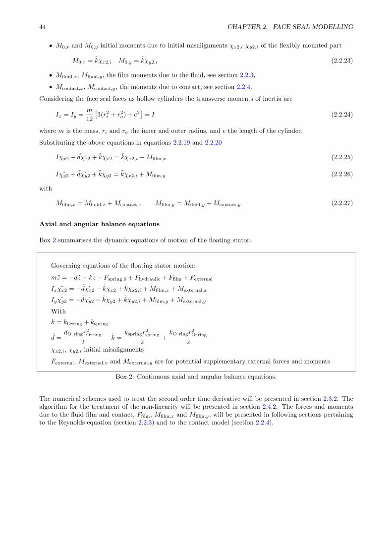
44 CHAPTER 2. FACE SEAL MODELLING
M0,x and M0,y initial moments due to initial misalignments χx2,i χy2,i of the flexibly mounted part
M0,x = kχx2,i M0,y = kχy2,i (2.2.23)
Mfluid,x, Mfluid,y, the film moments due to the fluid, see section 2.2.3,
Mcontact,x, Mcontact,y, the moments due to contact, see section 2.2.4.
Considering the face seal faces as hollow cylinders the transverse moments of inertia are
Ix = Iy =m
12
[3(r2
i + r2o) + e2
]= I (2.2.24)
where m is the mass, ri and ro the inner and outer radius, and e the length of the cylinder.
Substituting the above equations in equations 2.2.19 and 2.2.20
Iχx2 + d ˙χx2 + kχx2 = kχx2,i +Mfilm,x (2.2.25)
Iχy2 + d ˙χy2 + kχy2 = kχx2,i +Mfilm,y (2.2.26)
with
Mfilm,x = Mfluid,x +Mcontact,x Mfilm,y = Mfluid,y +Mcontact,y (2.2.27)
Axial and angular balance equations
Box 2 summarises the dynamic equations of motion of the floating stator.
Governing equations of the floating stator motion:
mz = −dz − kz − Fspring,0 + Fhydraulic + Ffilm + Fexternal
Ixχx2 = −d ˙χx2 − kχx2 + kχx2,i +Mfilm,x +Mexternal,x
Iyχy2 = −d ˙χy2 − kχy2 + kχy2,i +Mfilm,y +Mexternal,y
With
k = kO-ring + kspring
d =dO-ringr
2O-ring
2k =
kspringr2spring
2+kO-ringr
2O-ring
2χx2,i, χy2,i initial misalignments
Fexternal, Mexternal,x and Mexternal,y are for potential supplementary external forces and moments
Box 2: Continuous axial and angular balance equations.
The numerical schemes used to treat the second order time derivative will be presented in section 2.3.2. Thealgorithm for the treatment of the non-linearity will be presented in section 2.4.2. The forces and momentsdue to the fluid film and contact, Ffilm, Mfilm,x and Mfilm,y, will be presented in following sections pertainingto the Reynolds equation (section 2.2.3) and to the contact model (section 2.2.4).
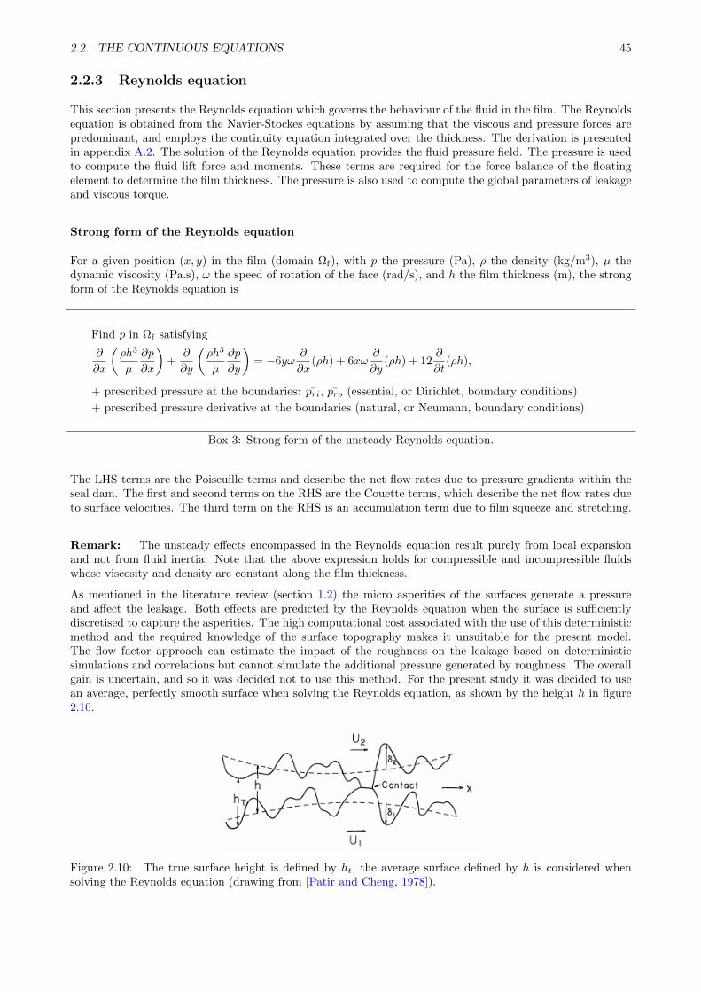
2.2. THE CONTINUOUS EQUATIONS 45
2.2.3 Reynolds equation
This section presents the Reynolds equation which governs the behaviour of the fluid in the film. The Reynoldsequation is obtained from the Navier-Stockes equations by assuming that the viscous and pressure forces arepredominant, and employs the continuity equation integrated over the thickness. The derivation is presentedin appendix A.2. The solution of the Reynolds equation provides the fluid pressure field. The pressure is usedto compute the fluid lift force and moments. These terms are required for the force balance of the floatingelement to determine the film thickness. The pressure is also used to compute the global parameters of leakageand viscous torque.
Strong form of the Reynolds equation
For a given position (x, y) in the film (domain Ωf), with p the pressure (Pa), ρ the density (kg/m3), µ thedynamic viscosity (Pa.s), ω the speed of rotation of the face (rad/s), and h the film thickness (m), the strongform of the Reynolds equation is
Find p in Ωf satisfying
∂
∂x
(ρh3
µ
∂p
∂x
)+
∂
∂y
(ρh3
µ
∂p
∂y
)= −6yω
∂
∂x(ρh) + 6xω
∂
∂y(ρh) + 12
∂
∂t(ρh),
+ prescribed pressure at the boundaries: pri, pro (essential, or Dirichlet, boundary conditions)
+ prescribed pressure derivative at the boundaries (natural, or Neumann, boundary conditions)
Box 3: Strong form of the unsteady Reynolds equation.
The LHS terms are the Poiseuille terms and describe the net flow rates due to pressure gradients within theseal dam. The first and second terms on the RHS are the Couette terms, which describe the net flow rates dueto surface velocities. The third term on the RHS is an accumulation term due to film squeeze and stretching.
Remark: The unsteady effects encompassed in the Reynolds equation result purely from local expansionand not from fluid inertia. Note that the above expression holds for compressible and incompressible fluidswhose viscosity and density are constant along the film thickness.
As mentioned in the literature review (section 1.2) the micro asperities of the surfaces generate a pressureand affect the leakage. Both effects are predicted by the Reynolds equation when the surface is sufficientlydiscretised to capture the asperities. The high computational cost associated with the use of this deterministicmethod and the required knowledge of the surface topography makes it unsuitable for the present model.The flow factor approach can estimate the impact of the roughness on the leakage based on deterministicsimulations and correlations but cannot simulate the additional pressure generated by roughness. The overallgain is uncertain, and so it was decided not to use this method. For the present study it was decided to usean average, perfectly smooth surface when solving the Reynolds equation, as shown by the height h in figure2.10.
Figure 2.10: The true surface height is defined by ht, the average surface defined by h is considered whensolving the Reynolds equation (drawing from [Patir and Cheng, 1978]).
46 CHAPTER 2. FACE SEAL MODELLING
To solve the Reynolds equation, the film thickness h, its time variation, the face velocity ω, and the fluid char-acteristics µ, ρ are required. Sections 2.2.3 and 2.2.3 below show how the density and viscosity are estimated.
Evaluation of the density
In practical applications of a liquid face seal, the film may break, leading to a varying density if
the fluid is stretched due to the seal motion, or
the fluid pressure become lower than the cavitation pressure leading to vaporisation, or
some surrounding air is sucked into the seal, or
some dissolved gas is released when the pressure decreases (especially with mineral oils).
In these cases, a closure is needed for the density.
The Elrod-Adams algorithm [Elrod, 1981] relying on the Jakobson, Floberg and Olsson (JFO) model, is astandard cavitation model. The JFO theory divides the flow into zones of full film and full cavitation. TheReynolds equation governs the flow in the full film regions, whilst the pressure in the cavitated regions isassumed equal to the cavitation pressure and it is the density that varies. Elrod developed an algorithm whichconsiders all JFO conditions in a single Reynolds equation. This model, or a similar one, was used in e.g.[Lebeck, 1991; Salant and Homiller, 1992; Hirayama et al., 2004]
Another method relying on a homogeneous formulation was proposed by [Brunetiere and Wang, 2011] andused in, e.g. [Brunetiere, 2018]. This method has the advantage of being continuous, smooth, and inexpensive,while reproducing the results of the JFO model. The homogeneous method is used in the present work. Theessence of this model is to consider a permanent liquid-gas mixture where the gas phase takes the form ofbubbles cohabiting with the liquid phase. The density is
ρ =1
1− λρl
+λ
ρg
(2.2.28)
with λ the gas mass fraction, which can be fixed to a small value, computed using saturation data if gas releaseis considered or computed using energy balance if vaporisation is considered. As a default, λ can be consideredto be ∈
[10−7; 10−5
]. The liquid density ρl is assumed constant.
The gas density ρg is related to the pressure with an equation of state. In an initial approach, the perfect gaslaw can be used
ρg =p
rgasT(2.2.29)
with rgas the gas constant. When air is considered, rgas = 287 J ·K−1 · kg−1.
Evaluation of the viscosity
Saadat and Flint [1996] showed that the McAdams law is accurate to estimate the viscosity of mixtures
µ =1
1− λµl
+λ
µg
(2.2.30)
Here, µl is the viscosity of the liquid and µg that of the gas. Such a law is used in other works on mechanicalface seals, such as [Brunetiere, 2016, 2018]. µg and µl are assumed to be only temperature dependent and tofollow the Reynolds model [Reynolds, 1886]
µl(T ) = µ(T0) exp(bvisc(T − T0)) (2.2.31)
where bvisc, in K−1, is the coefficient of thermo-viscosity, which can be estimated using a temperature superiorto T , T1 and its associated viscosity µ1
bvisc = ln(µ0
µ1)/(T1 − T0) (2.2.32)
More details on viscosity and its dependence on temperature can be found in, e.g. [Stachowiak and Batchelor,2014] or [Hamrock et al., 2004].
2.2. THE CONTINUOUS EQUATIONS 47
Outputs of the solution of the Reynolds equation
The solution of the Reynolds equation provides the pressure field which allows determining the intrinsic sealparameters: the fluid velocity, and shear rate, as well as the global parameters: the leakage, viscous torque,and the fluid film forces and moments.
Leakage
The face seal leakage is the flow of fluid through the outer (or inner) radius. As a mass flow, it equals thedensity times the velocity of the fluid projected onto the normal to the surface times the surface
m =
∫h
∫θ
ρ(unx + vny)rdθdh (2.2.33)
with nx and ny the components of the normal to the surface S. Here, u and v are the fluid velocities and areknown when the pressure is determined, see appendix A.2.
Shear stress
The shearing of the fluid dissipates or transforms some of the energy of the fluid momentum into heat. Fluidshearing is due to the friction of superposed fluid layers of different speeds. The shear stress is given by
τyz = µ∂v
∂zτxz = µ
∂u
∂z(2.2.34)
Based on equations A.2.15 and A.2.16 of appendix A.2 and with U2, V2 the speeds of the surface
τxz =1
2
∂p
∂xh+ µ
U2
hτyz =
1
2
∂p
∂yh+ µ
V2
h(2.2.35)
Local viscous heat generation
The shear stresses are used to estimate the local viscous heat generation qvisc
qvisc(x, y) = ω(xτyz − yτxz) (2.2.36)
Face seal viscous torque
At a global level, the force generated by fluid shearing τxydS times the distance to the rotating axis producesa viscous resisting torque
Tvisc =
∫∫x,y
(xτyz − yτxz)dxdy (2.2.37)
Global power
The overall power dissipated by viscous friction is directly obtained from the torque
P = ωTvisc (2.2.38)
Fluid forces and moments
The lift fluid force due to the fluid is obtained by integrating the fluid pressure
F =
∫S
pdS (2.2.39)
The moments are obtained using
Mx =
∫S
pydS (2.2.40)
My = −∫S
pxdS (2.2.41)
The last three equations are direct inputs to the force and moment balance solver (see box 8 in section 2.2.2).The contact forces and moments which are also input to the dynamic solid solver will be presented in the nextsection.
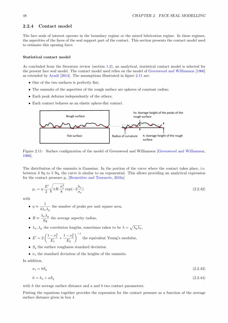
48 CHAPTER 2. FACE SEAL MODELLING
2.2.4 Contact model
The face seals of interest operate in the boundary regime or the mixed lubrication regime. In these regimes,the asperities of the faces of the seal support part of the contact. This section presents the contact model usedto estimate this opening force.
Statistical contact model
As concluded from the literature review (section 1.2), an analytical, statistical contact model is selected forthe present face seal model. The contact model used relies on the model of Greenwood and Williamson [1966]as extended by Ayadi [2014]. The assumptions illustrated in figure 2.11 are:
One of the two surfaces is perfectly flat;
The summits of the asperities of the rough surface are spheres of constant radius;
Each peak deforms independently of the others;
Each contact behaves as an elastic sphere-flat contact.
Flat surface h: Average height of the rough surface
hs: Average height of the peaks of the rough surface Rough surface
Radius of curvature
Figure 2.11: Surface configuration of the model of Greenwood and Williamson [Greenwood and Williamson,1966].
The distribution of the summits is Gaussian. In the portion of the curve where the contact takes place, i.e.between 3 Sq to 5 Sq, the curve is similar to an exponential. This allows providing an analytical expressionfor the contact pressure pc [Brunetiere and Tournerie, 2016a]
pc = ηE′
2
√πR
σ3s
8exp(−2
hsσs
) (2.2.42)
with
η ≈ 1
4λxλythe number of peaks per unit square area,
R ≈ λxλySq
the average asperity radius,
λx, λy the correlation lengths, sometimes taken to be λ =√λyλx,
E′ = 2
(1− ν2
1
E1+
1− ν22
E2
)−1
the equivalent Young’s modulus,
Sq the surface roughness standard deviation
σs the standard deviation of the heights of the summits.
In addition,
σs = bSq (2.2.43)
h = hs + aSq (2.2.44)
with h the average surface distance and a and b two contact parameters.
Putting the equations together provides the expression for the contact pressure as a function of the averagesurface distance given in box 4
2.2. THE CONTINUOUS EQUATIONS 49
Equation for the contact pressure as a function of the average face distance
pc(h) =E′
8λSq
√π
8b1.5 exp(
2a
b) exp(− 2h
bSq)
Box 4: Explicit contact equation.
pc(h) =E′
8λSq
√π
8exp(1) exp(−2h
Sq) (2.2.45)
The correlation length λ and the standard deviation of the roughness of the surface Sq are obtained frommeasuring the topography of the surfaces. The representative values are determined using
Sq =√S2q,1 + S2
q,2 (2.2.46)
λ =
(1
λ1+
1
λ2
)−1
(2.2.47)
The contact parameters a and b are used to tune the contact model to specific surfaces. Minet et al. [2010]compared the contact pressure of a face seal obtained with a statistical contact model and with his deterministiccontact model and observed that 0.2 < a < 1.1 and 0.4 < b < 1.2. Ayadi [2014] obtained a = 1.13 and b = 0.37while Brunetiere and Tournerie [2016a] propose a default value of a = 0.5 and b = 1.0. Based on several teststhe parameters a = 0.5 and b = 1.0 are used in this thesis. Appendix A.3 presents a parametric studyhighlighting the impact of the variation of varying a and b.
Outputs from the computation of the contact pressure
The contact pressure pc is used to compute the following outputs:
Global contact force
Fcontact =
∫S
pcdS (2.2.48)
Global moments due to contact
Mcontact,x =
∫S
pcydS Mcontact,y = −∫S
pcxdS (2.2.49)
Global dry torque Tdry and power dissipated by friction Pc
Tdry =
∫∫x,y
fpc√x2 + y2dS Pc = ωTdry (2.2.50)
Local heat generation due to dry friction, with f the friction coefficient
qdry(x, y) = fpcω√x2 + y2 (2.2.51)
2.2.5 Energy equations and thermo-mechanical deformation equations
This section presents the equations used to compute the temperature of the solids and fluid and the thermo-mechanical deformations. The temperature in the solids is used to determine the thermal deformations of thesolids, which directly affect the film thickness. The temperature field in the liquid is used to determine theviscosity, which directly affects the leakage, heat generation, and torque.
As concluded from the literature review section, see section 1.2.2, it was decided to integrate a thermo-mechanical module in the face seal model. This includes a temperature and a thermo-mechanical equationsolved in the parts of the face seal.
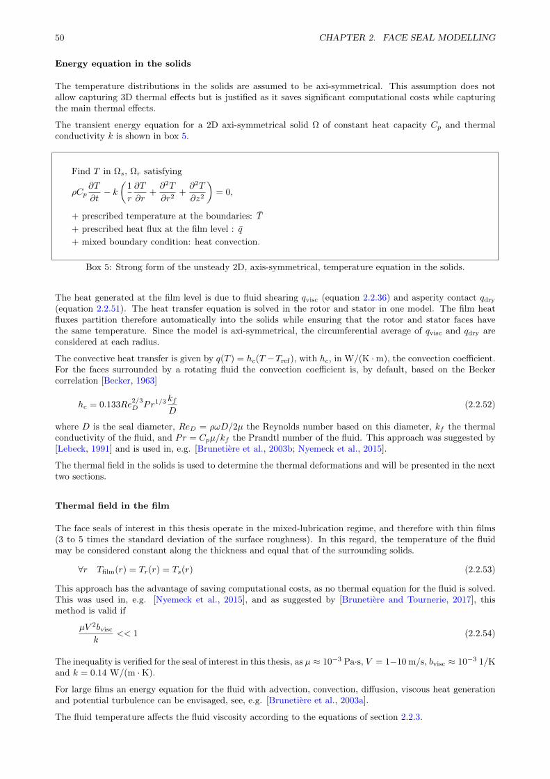
50 CHAPTER 2. FACE SEAL MODELLING
Energy equation in the solids
The temperature distributions in the solids are assumed to be axi-symmetrical. This assumption does notallow capturing 3D thermal effects but is justified as it saves significant computational costs while capturingthe main thermal effects.
The transient energy equation for a 2D axi-symmetrical solid Ω of constant heat capacity Cp and thermalconductivity k is shown in box 5.
Find T in Ωs, Ωr satisfying
ρCp∂T
∂t− k
(1
r
∂T
∂r+∂2T
∂r2+∂2T
∂z2
)= 0,
+ prescribed temperature at the boundaries: T
+ prescribed heat flux at the film level : q
+ mixed boundary condition: heat convection.
Box 5: Strong form of the unsteady 2D, axis-symmetrical, temperature equation in the solids.
The heat generated at the film level is due to fluid shearing qvisc (equation 2.2.36) and asperity contact qdry
(equation 2.2.51). The heat transfer equation is solved in the rotor and stator in one model. The film heatfluxes partition therefore automatically into the solids while ensuring that the rotor and stator faces havethe same temperature. Since the model is axi-symmetrical, the circumferential average of qvisc and qdry areconsidered at each radius.
The convective heat transfer is given by q(T ) = hc(T −Tref), with hc, in W/(K ·m), the convection coefficient.For the faces surrounded by a rotating fluid the convection coefficient is, by default, based on the Beckercorrelation [Becker, 1963]
hc = 0.133Re2/3D Pr1/3 kf
D(2.2.52)
where D is the seal diameter, ReD = ρωD/2µ the Reynolds number based on this diameter, kf the thermalconductivity of the fluid, and Pr = Cpµ/kf the Prandtl number of the fluid. This approach was suggested by[Lebeck, 1991] and is used in, e.g. [Brunetiere et al., 2003b; Nyemeck et al., 2015].
The thermal field in the solids is used to determine the thermal deformations and will be presented in the nexttwo sections.
Thermal field in the film
The face seals of interest in this thesis operate in the mixed-lubrication regime, and therefore with thin films(3 to 5 times the standard deviation of the surface roughness). In this regard, the temperature of the fluidmay be considered constant along the thickness and equal that of the surrounding solids.
∀r Tfilm(r) = Tr(r) = Ts(r) (2.2.53)
This approach has the advantage of saving computational costs, as no thermal equation for the fluid is solved.This was used in, e.g. [Nyemeck et al., 2015], and as suggested by [Brunetiere and Tournerie, 2017], thismethod is valid if
µV 2bvisc
k<< 1 (2.2.54)
The inequality is verified for the seal of interest in this thesis, as µ ≈ 10−3 Pa·s, V = 1−10 m/s, bvisc ≈ 10−3 1/Kand k = 0.14 W/(m ·K).
For large films an energy equation for the fluid with advection, convection, diffusion, viscous heat generationand potential turbulence can be envisaged, see, e.g. [Brunetiere et al., 2003a].
The fluid temperature affects the fluid viscosity according to the equations of section 2.2.3.
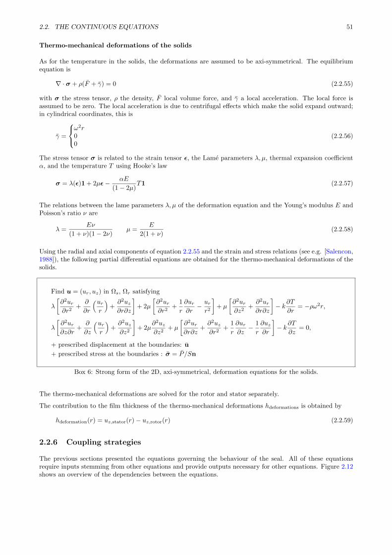
2.2. THE CONTINUOUS EQUATIONS 51
Thermo-mechanical deformations of the solids
As for the temperature in the solids, the deformations are assumed to be axi-symmetrical. The equilibriumequation is
∇ · σ + ρ(F + γ) = 0 (2.2.55)
with σ the stress tensor, ρ the density, F local volume force, and γ a local acceleration. The local force isassumed to be zero. The local acceleration is due to centrifugal effects which make the solid expand outward;in cylindrical coordinates, this is
γ =
ω2r
00
(2.2.56)
The stress tensor σ is related to the strain tensor ε, the Lame parameters λ, µ, thermal expansion coefficientα, and the temperature T using Hooke’s law
σ = λ(ε)1 + 2µε− αE
(1− 2µ)T1 (2.2.57)
The relations between the lame parameters λ, µ of the deformation equation and the Young’s modulus E andPoisson’s ratio ν are
λ =Eν
(1 + ν)(1− 2ν)µ =
E
2(1 + ν)(2.2.58)
Using the radial and axial components of equation 2.2.55 and the strain and stress relations (see e.g. [Salencon,1988]), the following partial differential equations are obtained for the thermo-mechanical deformations of thesolids.
Find u = (ur, uz) in Ωs, Ωr satisfying
λ
[∂2ur∂r2
+∂
∂r
(urr
)+∂2uz∂r∂z
]+ 2µ
[∂2ur∂r2
+1
r
∂ur∂r− urr2
]+ µ
[∂2ur∂z2
+∂2ur∂r∂z
]− k∂T
∂r= −ρω2r,
λ
[∂2ur∂z∂r
+∂
∂z
(urr
)+∂2uz∂z2
]+ 2µ
∂2uz∂z2
+ µ
[∂2ur∂r∂z
+∂2uz∂r2
+1
r
∂ur∂z− 1
r
∂uz∂r
]− k∂T
∂z= 0,
+ prescribed displacement at the boundaries: u
+ prescribed stress at the boundaries : σ = P /Sn
Box 6: Strong form of the 2D, axi-symmetrical, deformation equations for the solids.
The thermo-mechanical deformations are solved for the rotor and stator separately.
The contribution to the film thickness of the thermo-mechanical deformations hdeformations is obtained by
hdeformation(r) = uz,stator(r)− uz,rotor(r) (2.2.59)
2.2.6 Coupling strategies
The previous sections presented the equations governing the behaviour of the seal. All of these equationsrequire inputs stemming from other equations and provide outputs necessary for other equations. Figure 2.12shows an overview of the dependencies between the equations.
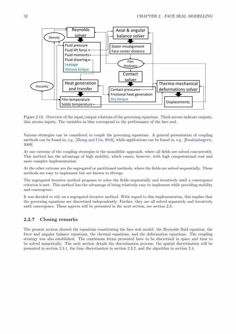
52 CHAPTER 2. FACE SEAL MODELLING
Reynolds solver
Fluid pressureFluid lift forceFluid momentsFluid shearingLeakageViscous torque
Heat generation and transfer
Film temperatureSolids temperature
Axial & angular balance solver
Contact solver
Thermo-mechanical deformations solver
Stator misalignmentFace center distance
Contact pressureFrictional heat generationDry torque
Displacements
Film thickness
Viscosity
Density
Figure 2.12: Overview of the input/output relations of the governing equations. Thick arrows indicate outputs,thin arrows inputs. The variables in blue correspond to the performance of the face seal.
Various strategies can be considered to couple the governing equations. A general presentation of couplingmethods can be found in, e.g. [Zhang and Cen, 2016], while applications can be found in, e.g. [Ibrahimbegovic,2009]
At one extreme of the coupling strategies is the monolithic approach, where all fields are solved concurrently.This method has the advantage of high stability, which comes, however, with high computational cost andmore complex implementation.
At the other extreme are the segregated or partitioned methods, where the fields are solved sequentially. Thesemethods are easy to implement but are known to diverge.
The segregated iterative method proposes to solve the fields sequentially and iteratively until a convergencecriterion is met. This method has the advantage of being relatively easy to implement while providing stabilityand convergence.
It was decided to rely on a segregated iterative method. With regard to this implementation, this implies thatthe governing equations are discretised independently. Further, they are all solved separately and iterativelyuntil convergence. These aspects will be presented in the next section, see section 2.3.
2.2.7 Closing remarks
The present section showed the equations constituting the face seal model: the Reynolds fluid equation, theforce and angular balance equations, the thermal equations, and the deformation equations. The couplingstrategy was also established. The continuous forms presented have to be discretised in space and time tobe solved numerically. The next section details the discretisation process: the spatial discretisation will bepresented in section 2.3.1, the time discretisation in section 2.3.2, and the algorithm in section 2.4.
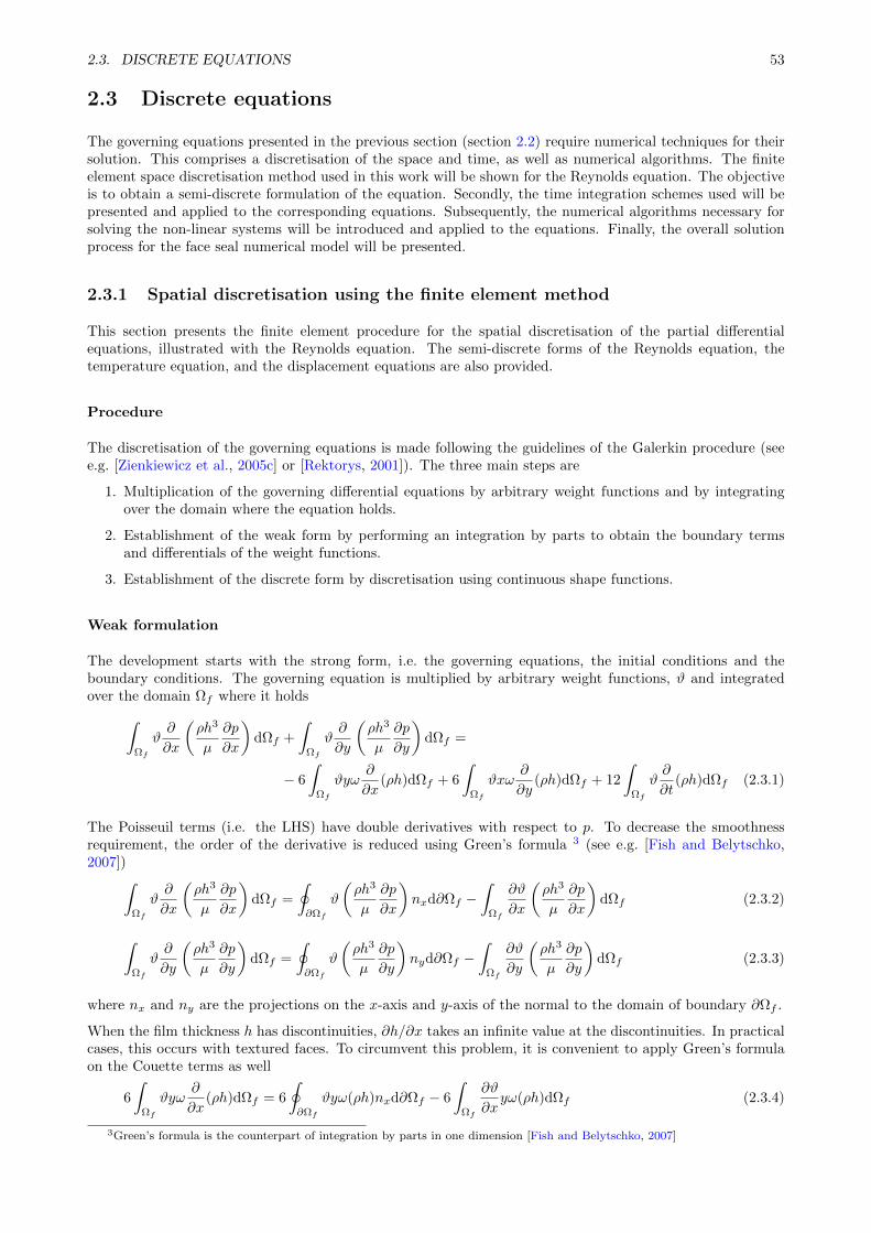
2.3. DISCRETE EQUATIONS 53
2.3 Discrete equations
The governing equations presented in the previous section (section 2.2) require numerical techniques for theirsolution. This comprises a discretisation of the space and time, as well as numerical algorithms. The finiteelement space discretisation method used in this work will be shown for the Reynolds equation. The objectiveis to obtain a semi-discrete formulation of the equation. Secondly, the time integration schemes used will bepresented and applied to the corresponding equations. Subsequently, the numerical algorithms necessary forsolving the non-linear systems will be introduced and applied to the equations. Finally, the overall solutionprocess for the face seal numerical model will be presented.
2.3.1 Spatial discretisation using the finite element method
This section presents the finite element procedure for the spatial discretisation of the partial differentialequations, illustrated with the Reynolds equation. The semi-discrete forms of the Reynolds equation, thetemperature equation, and the displacement equations are also provided.
Procedure
The discretisation of the governing equations is made following the guidelines of the Galerkin procedure (seee.g. [Zienkiewicz et al., 2005c] or [Rektorys, 2001]). The three main steps are
1. Multiplication of the governing differential equations by arbitrary weight functions and by integratingover the domain where the equation holds.
2. Establishment of the weak form by performing an integration by parts to obtain the boundary termsand differentials of the weight functions.
3. Establishment of the discrete form by discretisation using continuous shape functions.
Weak formulation
The development starts with the strong form, i.e. the governing equations, the initial conditions and theboundary conditions. The governing equation is multiplied by arbitrary weight functions, ϑ and integratedover the domain Ωf where it holds∫
Ωf
ϑ∂
∂x
(ρh3
µ
∂p
∂x
)dΩf +
∫Ωf
ϑ∂
∂y
(ρh3
µ
∂p
∂y
)dΩf =
− 6
∫Ωf
ϑyω∂
∂x(ρh)dΩf + 6
∫Ωf
ϑxω∂
∂y(ρh)dΩf + 12
∫Ωf
ϑ∂
∂t(ρh)dΩf (2.3.1)
The Poisseuil terms (i.e. the LHS) have double derivatives with respect to p. To decrease the smoothnessrequirement, the order of the derivative is reduced using Green’s formula 3 (see e.g. [Fish and Belytschko,2007])∫
Ωf
ϑ∂
∂x
(ρh3
µ
∂p
∂x
)dΩf =
∮∂Ωf
ϑ
(ρh3
µ
∂p
∂x
)nxd∂Ωf −
∫Ωf
∂ϑ
∂x
(ρh3
µ
∂p
∂x
)dΩf (2.3.2)
∫Ωf
ϑ∂
∂y
(ρh3
µ
∂p
∂y
)dΩf =
∮∂Ωf
ϑ
(ρh3
µ
∂p
∂y
)nyd∂Ωf −
∫Ωf
∂ϑ
∂y
(ρh3
µ
∂p
∂y
)dΩf (2.3.3)
where nx and ny are the projections on the x-axis and y-axis of the normal to the domain of boundary ∂Ωf .
When the film thickness h has discontinuities, ∂h/∂x takes an infinite value at the discontinuities. In practicalcases, this occurs with textured faces. To circumvent this problem, it is convenient to apply Green’s formulaon the Couette terms as well
6
∫Ωf
ϑyω∂
∂x(ρh)dΩf = 6
∮∂Ωf
ϑyω(ρh)nxd∂Ωf − 6
∫Ωf
∂ϑ
∂xyω(ρh)dΩf (2.3.4)
3Green’s formula is the counterpart of integration by parts in one dimension [Fish and Belytschko, 2007]
54 CHAPTER 2. FACE SEAL MODELLING
6
∫Ωf
ϑxω∂
∂y(ρh)dΩf = 6
∮∂Ωf
ϑxω(ρh)nyd∂Ωf − 6
∫Ωf
∂ϑ
∂yxω(ρh)dΩf (2.3.5)
Substituting equations 2.3.2, 2.3.3, 2.3.4 and 2.3.5 into equatiom 2.3.1 the weak form of the Reynolds equationis obtained
−∫
Ωf
∂ϑ
∂x
(ρh3
µ
∂p
∂x
)dΩf −
∫Ωf
∂ϑ
∂y
(ρh3
µ
∂p
∂y
)dΩf = −
∮∂Ωf
ϑ
(ρh3
µ
∂p
∂x
)nx∂Ωf −
∮∂Ωf
ϑ
(ρh3
µ
∂p
∂y
)nyd∂Ωf
+ 6
∫Ω
∂ϑ
∂xyω(ρh)dΩf − 6
∫Ωf
∂ϑ
∂yxω(ρh)dΩf
− 6
∮∂Ωf
ϑyω(ρh)nxd∂Ωf + 6
∮∂Ωf
ϑxω(ρh)nyd∂Ωf
+ 12
∫Ωf
ϑ∂
∂t(ρh)dΩf
(2.3.6)
Spatial discretisation
The idea of the finite element method is to split the domain Ω into ne non-overlapping sub-domains Ωe,referred to as elements. Each element has a defined number of nodes, and each node i has an associated shapefunction Ni.In finite element, each global continuous variable is approximated by the sum of its value at the node (nodalvariable) multiplied by the associated nodal shape function
p ≈nnode∑j=1
Njpj , (2.3.7)
This approximation is used for the unknown p, T,u and all the parameters h, µ, etc.. To help identifying thediscontinuous variable, such as the nodal pressure pj , they are not italicised by convention.
The approximation of equation 2.3.7 is applied to the weak form of the Reynolds equation. The nodal pressurepj are taken out of the integral and the error resulting from the approximations is gathered into a residual r
r =
nnode∑j=1
[∫Ωf
∂ϑ
∂x
(ρh3
µ
∂Nj∂x
)dΩfpj +
∫Ωf
∂ϑ
∂y
(ρh3
µ
∂Nj∂y
)dΩfpj
]
+ 6
∫Ωf
∂ϑ
∂xyωρhdΩf − 6
∫Ωf
∂ϑ
∂yxωρhdΩf
+ 12
∫Ωf
ϑ∂
∂t(hρ)dΩf
−∮∂Ωf
ϑ
(ρh3
µ
∂p
∂x
)nxd∂Ωf −
∮∂Ωf
ϑ
(ρh3
µ
∂p
∂y
)nyd∂Ωf
− 6
∮∂Ωf
ϑyω(ρh)nxd∂Ωf + 6
∮∂Ωf
ϑxω(ρh)nyd∂Ωf
(2.3.8)
As can be seen, there are nnode unknown pj . The weight functions have to be chosen so as to provide the same
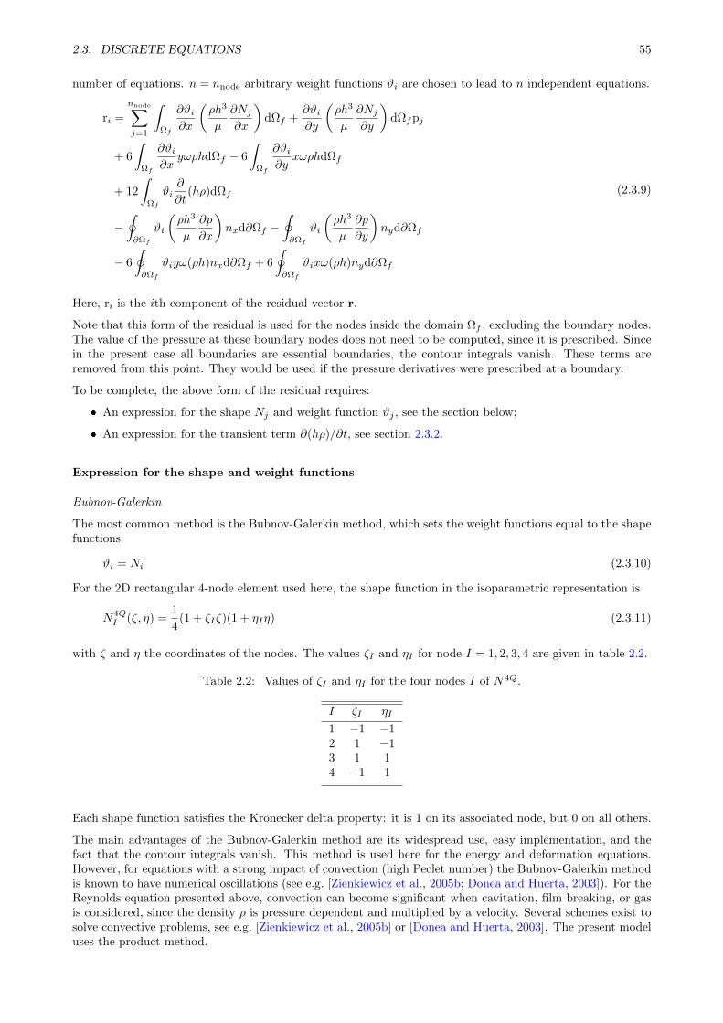
2.3. DISCRETE EQUATIONS 55
number of equations. n = nnode arbitrary weight functions ϑi are chosen to lead to n independent equations.
ri =
nnode∑j=1
∫Ωf
∂ϑi∂x
(ρh3
µ
∂Nj∂x
)dΩf +
∂ϑi∂y
(ρh3
µ
∂Nj∂y
)dΩfpj
+ 6
∫Ωf
∂ϑi∂x
yωρhdΩf − 6
∫Ωf
∂ϑi∂y
xωρhdΩf
+ 12
∫Ωf
ϑi∂
∂t(hρ)dΩf
−∮∂Ωf
ϑi
(ρh3
µ
∂p
∂x
)nxd∂Ωf −
∮∂Ωf
ϑi
(ρh3
µ
∂p
∂y
)nyd∂Ωf
− 6
∮∂Ωf
ϑiyω(ρh)nxd∂Ωf + 6
∮∂Ωf
ϑixω(ρh)nyd∂Ωf
(2.3.9)
Here, ri is the ith component of the residual vector r.
Note that this form of the residual is used for the nodes inside the domain Ωf , excluding the boundary nodes.The value of the pressure at these boundary nodes does not need to be computed, since it is prescribed. Sincein the present case all boundaries are essential boundaries, the contour integrals vanish. These terms areremoved from this point. They would be used if the pressure derivatives were prescribed at a boundary.
To be complete, the above form of the residual requires:
An expression for the shape Nj and weight function ϑj , see the section below;
An expression for the transient term ∂(hρ)/∂t, see section 2.3.2.
Expression for the shape and weight functions
Bubnov-Galerkin
The most common method is the Bubnov-Galerkin method, which sets the weight functions equal to the shapefunctions
ϑi = Ni (2.3.10)
For the 2D rectangular 4-node element used here, the shape function in the isoparametric representation is
N4QI (ζ, η) =
1
4(1 + ζIζ)(1 + ηIη) (2.3.11)
with ζ and η the coordinates of the nodes. The values ζI and ηI for node I = 1, 2, 3, 4 are given in table 2.2.
Table 2.2: Values of ζI and ηI for the four nodes I of N4Q.
I ζI ηI
1 −1 −12 1 −13 1 14 −1 1
Each shape function satisfies the Kronecker delta property: it is 1 on its associated node, but 0 on all others.
The main advantages of the Bubnov-Galerkin method are its widespread use, easy implementation, and thefact that the contour integrals vanish. This method is used here for the energy and deformation equations.However, for equations with a strong impact of convection (high Peclet number) the Bubnov-Galerkin methodis known to have numerical oscillations (see e.g. [Zienkiewicz et al., 2005b; Donea and Huerta, 2003]). For theReynolds equation presented above, convection can become significant when cavitation, film breaking, or gasis considered, since the density ρ is pressure dependent and multiplied by a velocity. Several schemes exist tosolve convective problems, see e.g. [Zienkiewicz et al., 2005b] or [Donea and Huerta, 2003]. The present modeluses the product method.
56 CHAPTER 2. FACE SEAL MODELLING
Upwinding scheme: product method
The Peclet number of the Reynolds equation can be defined as [Brunetiere, 2018]
Pe =3µ√U2V2Leρh2
∂ρ
∂p(2.3.12)
with Le a characteristic length of the element. Based on the method of [Heinrich et al., 1977], the upwindingfunctions are
L1 =1
2(1− ζ)− 3αζ
4(1− ζ)(1 + ζ) L2 =
1
2(1 + ζ)− 3αζ
4(1− ζ)(1 + ζ) (2.3.13)
with ζ the local coordinate of the element (resp. η) and αζ the upwinding coefficient, which varies between−1 and 1
αζ =1
Peζ− 1
tanh(Peζ)(2.3.14)
with Peζ the projection of the speed√U2V2 on the ζ direction.
Using a two-dimensional quadrangle, the upwinding functions in the (ζ, η) basis are [Brunetiere and Tournerie,2005]
N4Q,PROD1 (ζ, η) = L1(ζ)L1(η) N4Q,PROD
2 (ζ, η) = L2(ζ)L1(η)
N4Q,PROD3 (ζ, η) = L1(ζ)L2(η) N4Q,PROD
4 (ζ, η) = L2(ζ)L2(η)(2.3.15)
Note that if α = 0, the usual shape functions are recovered. This method was used in [Brunetiere, 2018, 2016]
Choice of weight and shape functions
For the energy and deformation equation, the Bubnov-Galerkin method is used with the shape functions N4Q.For the Reynolds equation, the Bubnov Galerkin method is used for all the weight functions and the desiredupwinding effect is obtained by using the product method (PROD) on (ρh) in the Couette term (i.e. convectiveterm).
(ρh) = (ρh)PROD =
nnode∑i
NPRODi (ρh)i (2.3.16)
Remark Expressing ρh with the product formulation may seem to contradict section 2.3.1, which indicatedthat the weight functions (and not the variables) are to be expressed with upwinding formulation. The issueis that if the product formulation were used on the weight function, the desired upwinding effect would becanceled for the 4Q element due to the derivative (except for a residual cross-derivative contribution). Theproduct formulation is used on the variable (and not the weight function) to ensure the upwinding effect. Thisapproach was successfully used in e.g. [Faria, 2001].
Semi-discrete form of the Reynolds equation
The space-discretised form of the Reynolds equation obtained using the above equations is given in box 7.
The semi-discrete form of the Reynolds equation is
ri = Kijpj − bi
with Kij and bi defined by equations 2.3.17 - 2.3.21.
Box 7: Semi-discrete form of the Reynolds equation.
Kij =
∫Ωf
∂Ni∂x
(ρh3
µ
∂Nj∂x
)dΩf +
∫Ωf
∂Ni∂y
(ρh3
µ
∂Nj∂y
)dΩf (2.3.17)
2.3. DISCRETE EQUATIONS 57
b1,i = −6
∫Ωf
∂Ni∂x
yω(ρh)PRODdΩf (2.3.18)
b2,i = 6
∫Ωf
∂Ni∂y
xω(ρh)PRODdΩf (2.3.19)
b3,i = +12
∫Ωf
Ni∂
∂t(hρ)dΩf (2.3.20)
bi = b1,i + b2,i + b3,i (2.3.21)
Equations 2.3.17 - 2.3.21 are the terms of the residual in equation 2.3.9 gathered into a matrix and vectors.
Semi-discrete form of the energy equation
The semi-discrete form of the energy equation obtained with a similar procedure is shown in appendix A.4. Itis of the form
Mij∂Tj∂t
+ KijTj − fT,i = 0 (2.3.22)
with Mij the mass matrix, Kij the stiffness matrix and fT,i the boundary term (see appendix A.4).
Semi-discrete form of the deformation equation
The semi-discrete form of the deformation equation obtained with a similar procedure is shown in appendixA.5. It is of the form[
krrij krzijkzrij kzzij
] [urjuzj
]=
[frifzi
](2.3.23)
with krrij , krzij , kzrij , and kzzij , the stiffness, and fri and fzi the boundary terms (see appendix A.5).
Note on implementation
Numerical integration
All the integrals are evaluated using Gauss quadrature. This method was chosen due to its ability to exactlyevaluate the integrals of polynomial functions, for details, see [Hughes, 2000].
Assembly
The indicial expression of the semi-discrete form has a matrix counterpart. For the Reynolds equation
r = Kp− b (2.3.24)
K is equivalent to a stiffness matrix and b to a source varying in time and depending on the unknown vectorp.
It is important to note that the global matrix - K and vectors r,p,b - are the sum of the contributions of allthe element-level vectors and matrices. Formally written, this assembly procedure is
r =
nb elt∑e=1
Lere (2.3.25)
and
K =
nb elt∑e=1
LTe KeLe (2.3.26)
where Le are the scatter matrices representing the assembling procedure. Implementation-wise, the assemblyis performed by adding the contributions of the various elements in the global matrix. More details on thisprocedure can be found in e.g. [Zienkiewicz et al., 2005b] or [Fish and Belytschko, 2007].
58 CHAPTER 2. FACE SEAL MODELLING
2.3.2 Time integration schemes
The next step is the discretisation of the time dependent terms: the first-order time derivative ∂ρh/∂t for theReynolds equation, the first-order time derivative ∂T/∂t for the energy equation, and first- and second-ordertime derivatives z, z, χx, χx, χy, χy for the axial and angular balance solver.
The time interval [t0, tmax] - where the equations are valid - is partitioned into time intervals [tj−1, tj ] of length∆t, where j is the index of the time step and tj denotes the unknown point in time sought. The value of thevariables at tj is determined from their values at time tj−1 through time integration schemes.
Schemes for first order differential equations
The generalised theta method, also referred to as the generalised trapezoidal method, can be found in, e.g.[Hughes, 2000]. Applying the generalized theta scheme to the energy equation yields
Mij
Ttj
j − Ttj−∆tj
∆t+ θKijT
tj
j + (1− θ)KijTtj−∆tj − θftjT,i − (1− θ)ftj−∆t
T,i = 0 (2.3.27)
with θ a parameter controlling the type of scheme, in particular,
θ = 0: explicit scheme,
θ = 1: implicit scheme,
0 < θ < 1: intermediate time integration schemes (e.g. mid-side Crank-Nicolson for θ = 0.5).
Setting for the energy equation θ = 1 to have an implicit scheme with first order precision and unconditionalstability yields
(1
∆tMij + Kij)T
tj =1
∆tMijT
tj−∆t + ftj
T,i (2.3.28)
The Reynolds equation is also discretised with the generalised theta scheme implicit (θ = 1). The residual is
rtj
i = KijPtj
j − bitj (2.3.29)
where btj
3,i of equation 2.3.21 is now
btj
3,i = 12
∫Ω
Ni∂hρ
∂tdΩ =
12
∆t
∫Ω
Ni(ρh)tj
dΩ− 12
∆t
∫Ω
Ni(ρh)tj−∆tdΩ (2.3.30)
Schemes for second order differential equations
Three different time integration schemes have been tested for second order partial differential equations: Eulerparabolic, Euler cubic and Generalized Newmark.
The parabolic Euler temporal scheme
The underlying idea of this scheme is to assume a parabolic, i.e. second order polynomial, evolution of thevariable
x(tj) = a(tj)2 + btj + c (2.3.31)
The associated derivatives are
∂x
∂t
∣∣∣∣tj
= 2atj + b (2.3.32)
∂2x
∂t2
∣∣∣∣tj
= 2a (2.3.33)
2.3. DISCRETE EQUATIONS 59
The parameters a, b need to be expressed as functions of x(tj−1) and x(tj−2) to obtain the derivative. x(t) isconsidered at ∆t, 0, and −∆t (which is equivalent to tj , tj−1, and tj−2 with tj−1 = 0)
x(∆t) = a(∆t)2 + b∆t+ c
x(0) = c
x(−∆t) = a(∆t)2 − b∆t+ c
(2.3.34)
The parameters a, b, and c are deduced from equations 2.3.34. The derivatives are thus
∂x
∂t
∣∣∣∣tj
=3x(t)− 4x(tj−1) + x(tj−2)
2∆t(2.3.35)
∂2x
∂t2
∣∣∣∣tj
=x(t)− 2x(tj−1) + x(tj−2)
∆t2(2.3.36)
In the next sub-section, a cubic scheme will be derived in the same fashion. The cubic scheme has one moreequation, but, unlike the parabolic scheme, allows a variation of the acceleration within the time step.
The cubic Euler temporal scheme
The variable x(t) is assumed to evolve as
x(tj) = a(tj)3 + b(tj)2 + c(tj) + d (2.3.37)
The associated derivatives are
∂x
∂t
∣∣∣∣tj
= 3a(tj)2 + 2b∆t+ c (2.3.38)
∂2x
∂t2
∣∣∣∣tj
= 6atj + 2b (2.3.39)
In the same fashion as for the parabolic scheme, the parameters a, b, c, and d need to be expressed as functionsof x(tj−1), x(tj−2), and x(tj−3) to obtain the derivatives. x(t) is considered at ∆t, 0, −∆t, and −2∆t (whichis equivalent to tj , tj−1, tj−2, and tj−3 with tj−1 = 0)
x(∆t) = a(∆t)3 + b(∆t)2 + c(∆t) + d
x(0) = d
x(−∆t) = −a(∆t)3 + b(∆t)2 − c(∆t) + d
x(−2∆t) = −8a(∆t)3 + 4b(∆t)2 − c(∆t) + d
(2.3.40)
The parameters are
a = −x(−2∆t)− x(∆t) + 3x(0)− 3(−∆t)
6∆t3
b =x(∆t) + x(−∆t)− 2x(0)
2∆t2
c =2x(∆t) + x(−2∆t) + 3x(0)− 6x(−∆t)
6∆td = x(0)
(2.3.41)
Consequently
∂x
∂t
∣∣∣∣tj
=−2x(tj−3) + 11x(tj)− 18x(tj−1) + 9x(tj−2)
6∆t(2.3.42)
∂2x
∂t2
∣∣∣∣tj
=−x(tj−3) + 2x(tj)− 5x(tj−1) + 4x(tj−2)
∆t2(2.3.43)
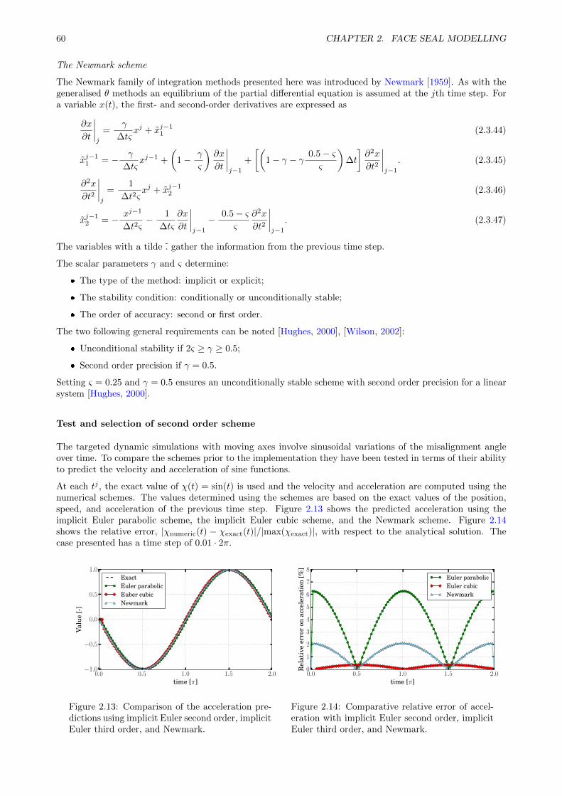
60 CHAPTER 2. FACE SEAL MODELLING
The Newmark scheme
The Newmark family of integration methods presented here was introduced by Newmark [1959]. As with thegeneralised θ methods an equilibrium of the partial differential equation is assumed at the jth time step. Fora variable x(t), the first- and second-order derivatives are expressed as
∂x
∂t
∣∣∣∣j
=γ
∆tςxj + xj−1
1 (2.3.44)
xj−11 = − γ
∆tςxj−1 +
(1− γ
ς
)∂x
∂t
∣∣∣∣j−1
+
[(1− γ − γ 0.5− ς
ς
)∆t
]∂2x
∂t2
∣∣∣∣j−1
. (2.3.45)
∂2x
∂t2
∣∣∣∣j
=1
∆t2ςxj + xj−1
2 (2.3.46)
xj−12 = − xj−1
∆t2ς− 1
∆tς
∂x
∂t
∣∣∣∣j−1
− 0.5− ςς
∂2x
∂t2
∣∣∣∣j−1
. (2.3.47)
The variables with a tilde . gather the information from the previous time step.
The scalar parameters γ and ς determine:
The type of the method: implicit or explicit;
The stability condition: conditionally or unconditionally stable;
The order of accuracy: second or first order.
The two following general requirements can be noted [Hughes, 2000], [Wilson, 2002]:
Unconditional stability if 2ς ≥ γ ≥ 0.5;
Second order precision if γ = 0.5.
Setting ς = 0.25 and γ = 0.5 ensures an unconditionally stable scheme with second order precision for a linearsystem [Hughes, 2000].
Test and selection of second order scheme
The targeted dynamic simulations with moving axes involve sinusoidal variations of the misalignment angleover time. To compare the schemes prior to the implementation they have been tested in terms of their abilityto predict the velocity and acceleration of sine functions.
At each tj , the exact value of χ(t) = sin(t) is used and the velocity and acceleration are computed using thenumerical schemes. The values determined using the schemes are based on the exact values of the position,speed, and acceleration of the previous time step. Figure 2.13 shows the predicted acceleration using theimplicit Euler parabolic scheme, the implicit Euler cubic scheme, and the Newmark scheme. Figure 2.14shows the relative error, |χnumeric(t) − χexact(t)|/|max(χexact)|, with respect to the analytical solution. Thecase presented has a time step of 0.01 · 2π.
0.0 0.5 1.0 1.5 2.0time [π]
−1.0
−0.5
0.0
0.5
1.0
Valu
e[-
]
ExactEuler parabolicEuber cubicNewmark
Figure 2.13: Comparison of the acceleration pre-dictions using implicit Euler second order, implicitEuler third order, and Newmark.
0.0 0.5 1.0 1.5 2.0time [π]
0
1
2
3
4
5
6
7
8
Rel
ativ
eer
ror
onac
cele
rati
on[%
]
Euler parabolicEuler cubicNewmark
Figure 2.14: Comparative relative error of accel-eration with implicit Euler second order, implicitEuler third order, and Newmark.
2.3. DISCRETE EQUATIONS 61
One sees that the relative error has a maximum of 6% for the Euler parabolic scheme, 2% for the Newmarkscheme, and is below 0.5% for the Euler cubic scheme. The Euler cubic time integration scheme was selecteddue to its better predictions and its relatively simple implementation.
Remark Alternative time integration schemes such as the generalized alpha Wilson [2002]; Hulbert andChung [1993]; Cottrell et al. [2009] were also considered, but not implemented.
Application of a second order time integration scheme to the axial and angular balance solver
Recall the axial equation presented in section 2.2.2
mz = −dz − kx− F0 + F (z, χx, χy) (2.3.48)
with, for compactness, F0 = Fspring − Fhydraulic and F (z, χx, χy) = Ffilm + Fexternal.
This equation being valid at all time instants, it is at t = tj
mzj = −dzj − kzj − F0 + F j(zj , χjz, χjy) (2.3.49)
Applying the Euler cubic equations 2.3.42 and 2.3.43 and re-ordering yields[2m
∆t2+
11
6
d
∆t+ k
]zj =
[5m
∆t2+ 3
d
∆t
]zj−1 +
[−4
m
∆t2− 3
2
d
∆t
]zj−2
+
[m
∆t2+
1
3
d
∆t
]zj−3 − F0 + F j(zj , χjz, χ
jy)
(2.3.50)
Similarly, for the angular equation
Ixχjx = −dχjx − kχjx +Mx,0 +M j
x(z, χx, χy) (2.3.51)
with, for compactness, Mx,0 = kχx2,i and M jx(z, χx, χy) = Mfilm,x +Mexternal,x[
2I
∆t2+
11
6
d
∆t+ k
]χjx =
[5I
∆t2+ 3
d
∆t
]χj−1x +
[−4
I
∆t2− 3
2
d
∆t
]χj−2x
+
[I
∆t2+
1
3
d
∆t
]χj−3x +Mx,0 +M j
x(z, χx, χy)
(2.3.52)
and equivalently for the y equation.
The three governing equations discretised in time using an implicit Euler cubic scheme can be put in thecompact matrix form shown in box 8 below.
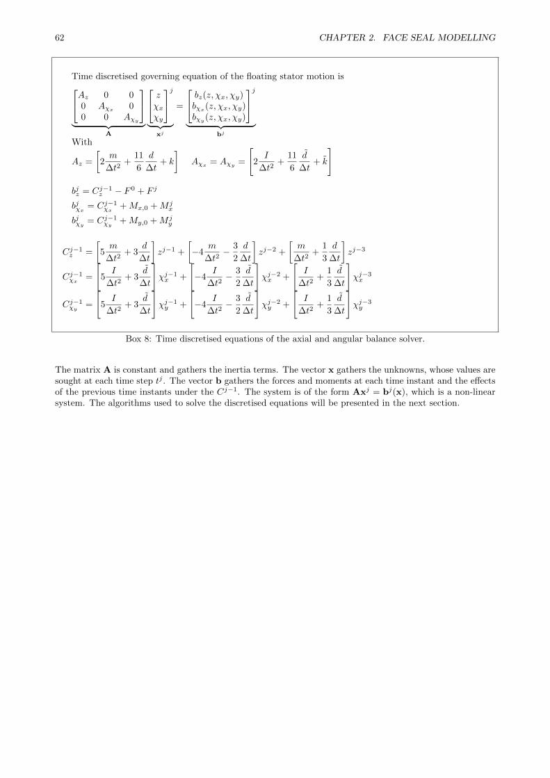
62 CHAPTER 2. FACE SEAL MODELLING
Time discretised governing equation of the floating stator motion isAz 0 00 Aχx
00 0 Aχy
︸ ︷︷ ︸
A
zχxχy
j︸ ︷︷ ︸
xj
=
bz(z, χx, χy)bχx
(z, χx, χy)bχy
(z, χx, χy)
j︸ ︷︷ ︸
bj
With
Az =
[2m
∆t2+
11
6
d
∆t+ k
]Aχx
= Aχy=
[2I
∆t2+
11
6
d
∆t+ k
]
bjz = Cj−1z − F 0 + F j
bjχx= Cj−1
χx+Mx,0 +M j
x
bjχy= Cj−1
χy+My,0 +M j
y
Cj−1z =
[5m
∆t2+ 3
d
∆t
]zj−1 +
[−4
m
∆t2− 3
2
d
∆t
]zj−2 +
[m
∆t2+
1
3
d
∆t
]zj−3
Cj−1χx
=
[5I
∆t2+ 3
d
∆t
]χj−1x +
[−4
I
∆t2− 3
2
d
∆t
]χj−2x +
[I
∆t2+
1
3
d
∆t
]χj−3x
Cj−1χy
=
[5I
∆t2+ 3
d
∆t
]χj−1y +
[−4
I
∆t2− 3
2
d
∆t
]χj−2y +
[I
∆t2+
1
3
d
∆t
]χj−3y
Box 8: Time discretised equations of the axial and angular balance solver.
The matrix A is constant and gathers the inertia terms. The vector x gathers the unknowns, whose values aresought at each time step tj . The vector b gathers the forces and moments at each time instant and the effectsof the previous time instants under the Cj−1. The system is of the form Axj = bj(x), which is a non-linearsystem. The algorithms used to solve the discretised equations will be presented in the next section.
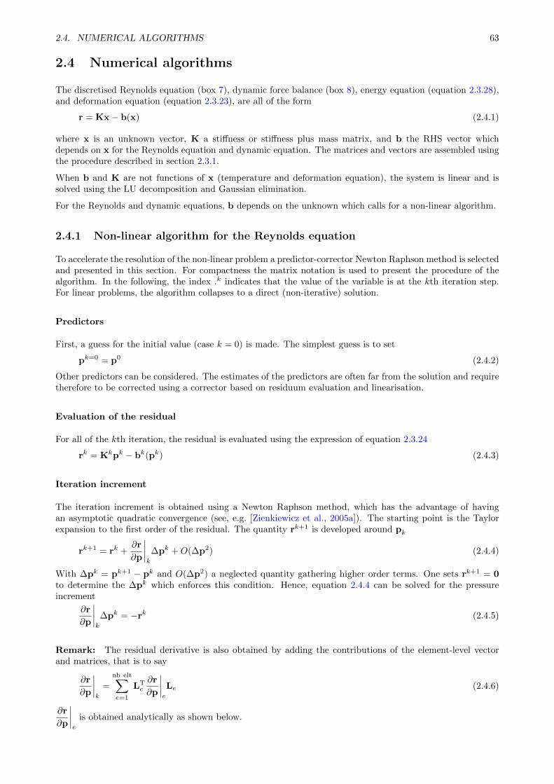
2.4. NUMERICAL ALGORITHMS 63
2.4 Numerical algorithms
The discretised Reynolds equation (box 7), dynamic force balance (box 8), energy equation (equation 2.3.28),and deformation equation (equation 2.3.23), are all of the form
r = Kx− b(x) (2.4.1)
where x is an unknown vector, K a stiffness or stiffness plus mass matrix, and b the RHS vector whichdepends on x for the Reynolds equation and dynamic equation. The matrices and vectors are assembled usingthe procedure described in section 2.3.1.
When b and K are not functions of x (temperature and deformation equation), the system is linear and issolved using the LU decomposition and Gaussian elimination.
For the Reynolds and dynamic equations, b depends on the unknown which calls for a non-linear algorithm.
2.4.1 Non-linear algorithm for the Reynolds equation
To accelerate the resolution of the non-linear problem a predictor-corrector Newton Raphson method is selectedand presented in this section. For compactness the matrix notation is used to present the procedure of thealgorithm. In the following, the index .k indicates that the value of the variable is at the kth iteration step.For linear problems, the algorithm collapses to a direct (non-iterative) solution.
Predictors
First, a guess for the initial value (case k = 0) is made. The simplest guess is to set
pk=0 = p0 (2.4.2)
Other predictors can be considered. The estimates of the predictors are often far from the solution and requiretherefore to be corrected using a corrector based on residuum evaluation and linearisation.
Evaluation of the residual
For all of the kth iteration, the residual is evaluated using the expression of equation 2.3.24
rk = Kkpk − bk(pk) (2.4.3)
Iteration increment
The iteration increment is obtained using a Newton Raphson method, which has the advantage of havingan asymptotic quadratic convergence (see, e.g. [Zienkiewicz et al., 2005a]). The starting point is the Taylorexpansion to the first order of the residual. The quantity rk+1 is developed around pk
rk+1 = rk +∂r
∂p
∣∣∣∣k
∆pk +O(∆p2) (2.4.4)
With ∆pk = pk+1 − pk and O(∆p2) a neglected quantity gathering higher order terms. One sets rk+1 = 0to determine the ∆pk which enforces this condition. Hence, equation 2.4.4 can be solved for the pressureincrement
∂r
∂p
∣∣∣∣k
∆pk = −rk (2.4.5)
Remark: The residual derivative is also obtained by adding the contributions of the element-level vectorand matrices, that is to say
∂r
∂p
∣∣∣∣k
=
nb elt∑e=1
LTe
∂r
∂p
∣∣∣∣e
Le (2.4.6)
∂r
∂p
∣∣∣∣e
is obtained analytically as shown below.
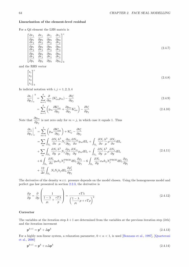
64 CHAPTER 2. FACE SEAL MODELLING
Linearization of the element-level residual
For a Q4 element the LHS matrix is
∂r1
∂p1
∂r1
∂p2
∂r1
∂p3
∂r1
∂p4∂r2
∂p1
∂r2
∂p2
∂r2
∂p3
∂r2
∂p4∂r3
∂p1
∂r3
∂p2
∂r3
∂p3
∂r3
∂p4∂r4
∂p1
∂r4
∂p2
∂r4
∂p3
∂r4
∂p4
e
k
(2.4.7)
and the RHS vectorr1
r2
r3
r4
e
k
(2.4.8)
In indicial notation with i, j = 1, 2, 3, 4
∂ri
∂pj
∣∣∣∣e
k
=
4∑m=1
∂
∂pj(Ke
impm)− ∂bei∂pj
(2.4.9)
=
4∑m=1
(pm
∂Keim
∂pj+∂pm∂pj
Keim
)− ∂bei∂pj
(2.4.10)
Note that∂pm∂pj
is not zero only for m = j, in which case it equals 1. Thus
∂ri∂pj
∣∣∣∣e
k
=
4∑m=1
(pm
∂Keim
∂pj
)+ Ke
ij −∂bei∂pj
=∑m
∫Ωe
∂Ni∂x
h3
µNj
∂ρj∂pj
∂Nm∂x
pmdΩe +
∫Ωe
∂Ni∂x
h3
µρ∂Nj∂x
dΩe
+∑m
∫Ωe
∂Ni∂y
h3
µNj
∂ρj∂pj
∂Nm∂y
pmdΩe +
∫Ωe
∂Ni∂y
h3
µρ∂Nj∂y
dΩe
+ 6
∫Ωe
∂Ni
∂xyωhjN
PRODj dΩe
∂ρj∂pj− 6
∫Ωe
∂Ni
∂yxωhjN
PRODj dΩe
∂ρj∂pj
+12
∆t
∫Ωe
NiNjhjdΩe∂ρtj∂pj
(2.4.11)
The derivative of the density w.r.t. pressure depends on the model chosen. Using the homogeneous model andperfect gas law presented in section 2.2.3, the derivative is
∂ρ
∂p=
∂
∂p
1
1− λρl
+rTλ
p
=rTλ(
1− λρl
p+ rTρ
)2 (2.4.12)
Corrector
The variables at the iteration step k+ 1 are determined from the variables at the previous iteration step (kth)and the iteration increment
pk+1 = pk + ∆pk (2.4.13)
For a highly non-linear system, a relaxation parameter, 0 < α < 1, is used [Bonnans et al., 1997], [Quarteroniet al., 2000]
pk+1 = pk + α∆pk (2.4.14)
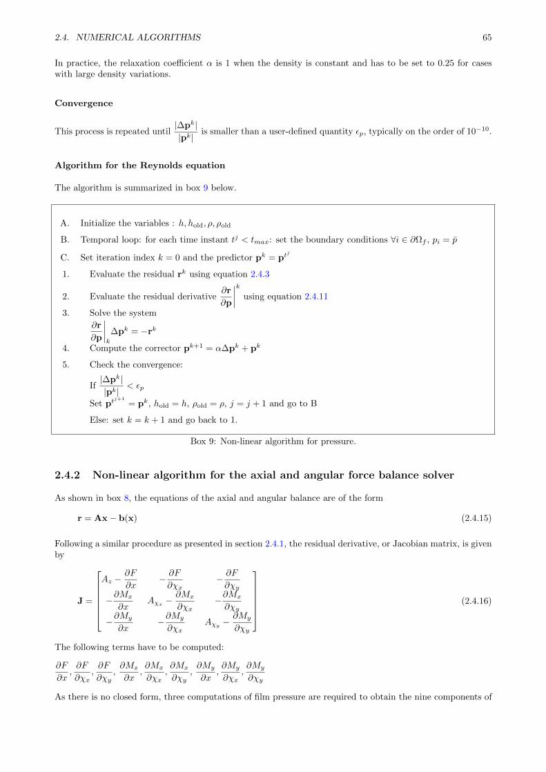
2.4. NUMERICAL ALGORITHMS 65
In practice, the relaxation coefficient α is 1 when the density is constant and has to be set to 0.25 for caseswith large density variations.
Convergence
This process is repeated until|∆pk||pk| is smaller than a user-defined quantity εp, typically on the order of 10−10.
Algorithm for the Reynolds equation
The algorithm is summarized in box 9 below.
A. Initialize the variables : h, hold, ρ, ρold
B. Temporal loop: for each time instant tj < tmax: set the boundary conditions ∀i ∈ ∂Ωf , pi = p
C. Set iteration index k = 0 and the predictor pk = ptj
1. Evaluate the residual rk using equation 2.4.3
2. Evaluate the residual derivative∂r
∂p
∣∣∣∣k using equation 2.4.11
3. Solve the system
∂r
∂p
∣∣∣∣k
∆pk = −rk
4. Compute the corrector pk+1 = α∆pk + pk
5. Check the convergence:
If|∆pk||pk| < εp
Set ptj+1
= pk, hold = h, ρold = ρ, j = j + 1 and go to B
Else: set k = k + 1 and go back to 1.
Box 9: Non-linear algorithm for pressure.
2.4.2 Non-linear algorithm for the axial and angular force balance solver
As shown in box 8, the equations of the axial and angular balance are of the form
r = Ax− b(x) (2.4.15)
Following a similar procedure as presented in section 2.4.1, the residual derivative, or Jacobian matrix, is givenby
J =
Az −
∂F
∂x− ∂F
∂χx− ∂F∂χy
−∂Mx
∂xAχx− ∂Mx
∂χx−∂Mx
∂χy
−∂My
∂x−∂My
∂χxAχy− ∂My
∂χy
(2.4.16)
The following terms have to be computed:
∂F
∂x,∂F
∂χx,∂F
∂χy,∂Mx
∂x,∂Mx
∂χx,∂Mx
∂χy,∂My
∂x,∂My
∂χx,∂My
∂χy
As there is no closed form, three computations of film pressure are required to obtain the nine components of
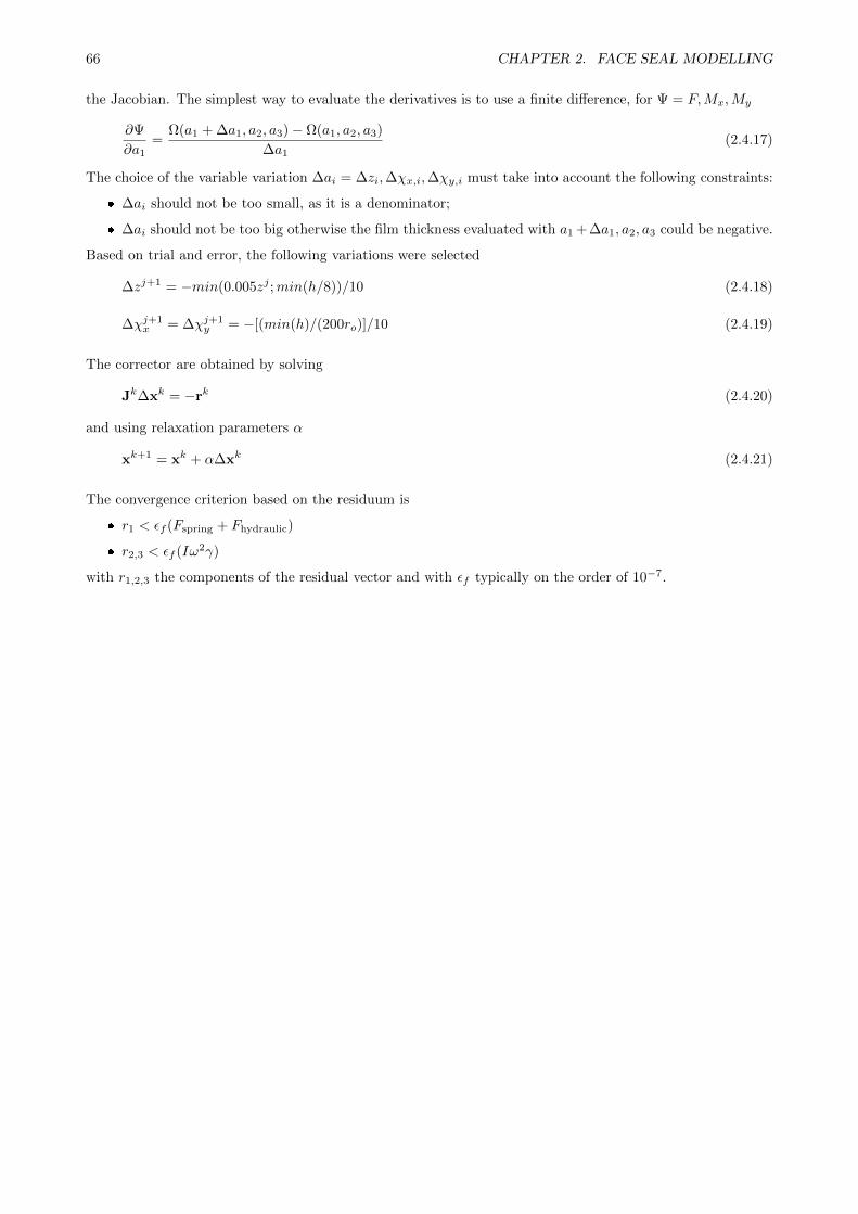
66 CHAPTER 2. FACE SEAL MODELLING
the Jacobian. The simplest way to evaluate the derivatives is to use a finite difference, for Ψ = F,Mx,My
∂Ψ
∂a1=
Ω(a1 + ∆a1, a2, a3)− Ω(a1, a2, a3)
∆a1(2.4.17)
The choice of the variable variation ∆ai = ∆zi,∆χx,i,∆χy,i must take into account the following constraints:
∆ai should not be too small, as it is a denominator;
∆ai should not be too big otherwise the film thickness evaluated with a1 + ∆a1, a2, a3 could be negative.
Based on trial and error, the following variations were selected
∆zj+1 = −min(0.005zj ;min(h/8))/10 (2.4.18)
∆χj+1x = ∆χj+1
y = −[(min(h)/(200ro)]/10 (2.4.19)
The corrector are obtained by solving
Jk∆xk = −rk (2.4.20)
and using relaxation parameters α
xk+1 = xk + α∆xk (2.4.21)
The convergence criterion based on the residuum is
r1 < εf (Fspring + Fhydraulic)
r2,3 < εf (Iω2γ)
with r1,2,3 the components of the residual vector and with εf typically on the order of 10−7.
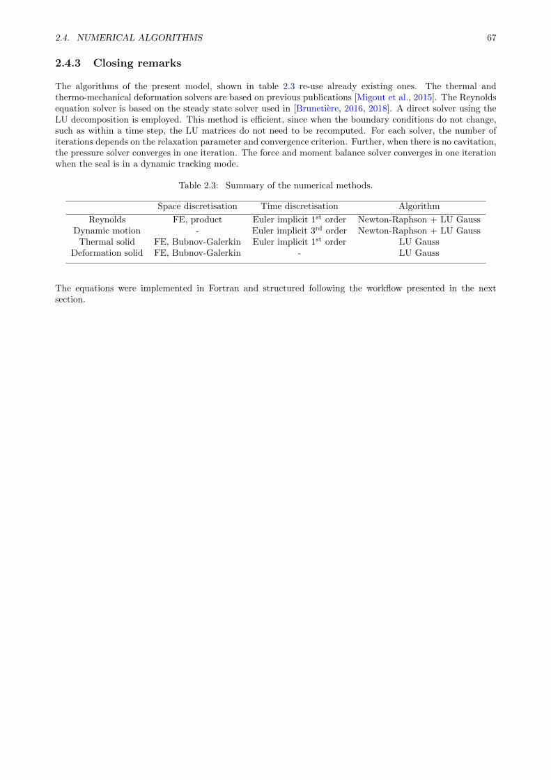
2.4. NUMERICAL ALGORITHMS 67
2.4.3 Closing remarks
The algorithms of the present model, shown in table 2.3 re-use already existing ones. The thermal andthermo-mechanical deformation solvers are based on previous publications [Migout et al., 2015]. The Reynoldsequation solver is based on the steady state solver used in [Brunetiere, 2016, 2018]. A direct solver using theLU decomposition is employed. This method is efficient, since when the boundary conditions do not change,such as within a time step, the LU matrices do not need to be recomputed. For each solver, the number ofiterations depends on the relaxation parameter and convergence criterion. Further, when there is no cavitation,the pressure solver converges in one iteration. The force and moment balance solver converges in one iterationwhen the seal is in a dynamic tracking mode.
Table 2.3: Summary of the numerical methods.
Space discretisation Time discretisation Algorithm
Reynolds FE, product Euler implicit 1st order Newton-Raphson + LU GaussDynamic motion - Euler implicit 3rd order Newton-Raphson + LU Gauss
Thermal solid FE, Bubnov-Galerkin Euler implicit 1st order LU GaussDeformation solid FE, Bubnov-Galerkin - LU Gauss
The equations were implemented in Fortran and structured following the workflow presented in the nextsection.
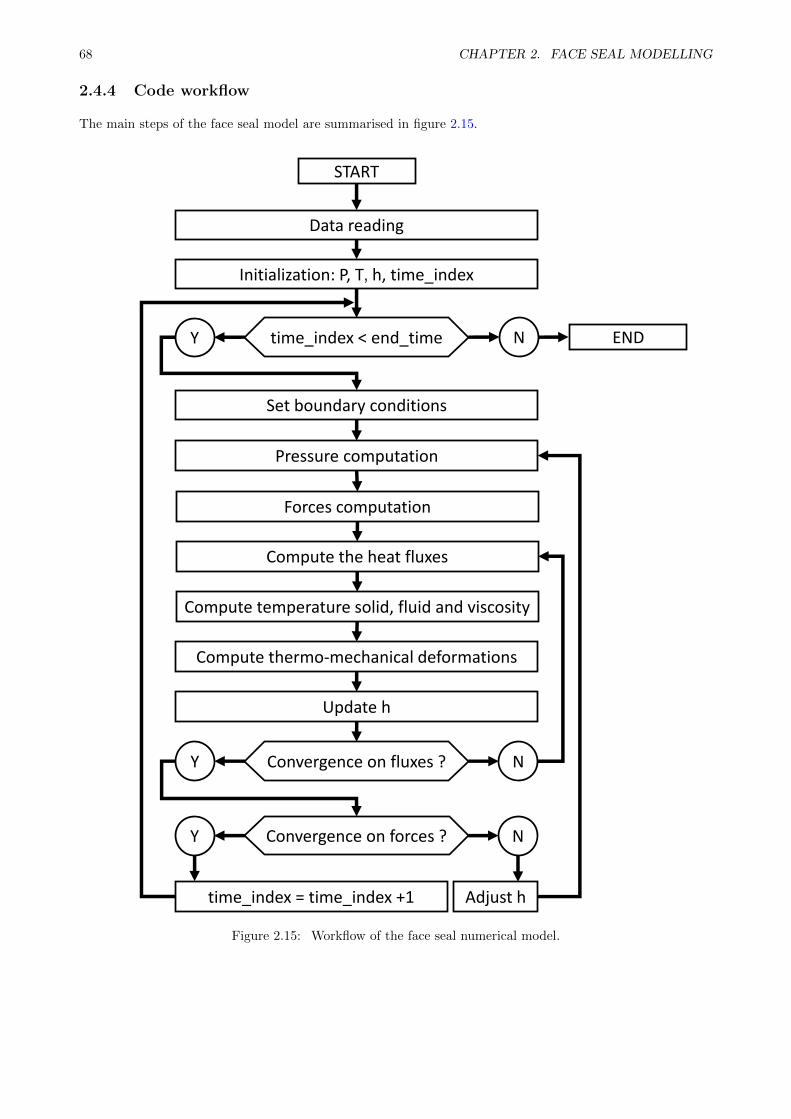
68 CHAPTER 2. FACE SEAL MODELLING
2.4.4 Code workflow
The main steps of the face seal model are summarised in figure 2.15.
START
Data reading
Initialization: P, T, h, time_index
Set boundary conditions
Pressure computation
Forces computation
Compute the heat fluxes
Adjust h
Compute temperature solid, fluid and viscosity
Compute thermo-mechanical deformations
Update h
Convergence on forces ?
Convergence on fluxes ? NY
NY
time_index = time_index +1
time_index < end_time NY END
Figure 2.15: Workflow of the face seal numerical model.
2.4. NUMERICAL ALGORITHMS 69
The convergence criteria are:
For the pressure|∆pk||pk| < εp with εp typically on the order of 10−10.
For the forces and moment balance:
– r1 < εf (Fspring + Fhydraulic)
– r2,3 < εf (Iω2γ)
with r1,2,3 the component of the residual vector and with εf typically on the order of 10−7.
For the heat fluxes|∆qk||qk| < εt with εt typically on the order of 10−6.
These criteria were selected based on a trial and error and on the values suggested in previous literature onthe Reynolds and thermo-mechanical solvers.
The code developed has been used to perform the simulations on face seals whose results will be presented inchapter 5. Chapter 3 will present a verification of the code, made by comparing its predictions to publishedresults, and a validation, made by a comparison with experimental data.
70 CHAPTER 2. FACE SEAL MODELLING
2.5 Summary of the face seal modelling strategy
This section presented the four main equations of the face seal numerical model:
The Reynolds equation for the motion of the fluid in the interface.
Newton’s second law for the dynamic motion of the floating stator. This equation is composed of anaxial force balance and two angular moment balances.
The unsteady, 2D axi-symmetrical thermal equation for the solids. The temperature of the fluid is setequal to the temperature of the solid.
The 2D axi-symmetrical deformation equation for the solids.
Further:
These coupled equations are solved sequentially and iteratively with a convergence criterion.
The Reynolds equation, as well as the thermal and deformation equations are discretised using the finiteelement method. A product upwinding method is used for the Reynolds equation.
The transient terms of the Reynolds equation and thermal equation are discretised using an implicit,first order, backward Euler scheme. An implicit Euler cubic scheme is used for the axial and angularbalance solver.
A Newton-Raphson algorithm is used for solving the non-linear Reynolds equation and axial and angularbalance equation.
Chapter 3
Comparison of the numerical modelwith published results
This chapter presents the comparisons made as part of the verification and validation of the numerical model.The verification aims at confirming the correct implementation of the solver, by comparing the predictions ofthe model to published results. The validation aims at demonstrating the validity of the assumptions of themodel, by comparing the predictions of the model to the relevant experimental data.
Contents3.1 Verification of the axial and angular balance solver . . . . . . . . . . . . . . . . . 72
3.1.1 Characterisation of misaligned face seals . . . . . . . . . . . . . . . . . . . . . . . . . 72
3.1.2 Comparison with the analytical model of Green and Etsion . . . . . . . . . . . . . . 72
3.1.3 Comparison with the dynamic tracking model of Person et al. . . . . . . . . . . . . . 74
3.1.4 Verification with the dynamic model of Tournerie and Frene . . . . . . . . . . . . . . 76
3.1.5 Conclusions about the verification of the dynamic solver . . . . . . . . . . . . . . . . 77
3.2 Verification of the thermal and deformation solver . . . . . . . . . . . . . . . . . 78
3.2.1 Verification of the thermal deformations . . . . . . . . . . . . . . . . . . . . . . . . . 78
3.2.2 Verification of unsteady thermal deformations . . . . . . . . . . . . . . . . . . . . . . 80
3.2.3 Conclusion about the verification of the thermal solver . . . . . . . . . . . . . . . . . 81
3.3 Comparison to the experimental data of Adjemout . . . . . . . . . . . . . . . . . 82
3.4 Summary of the numerical model verification and validation . . . . . . . . . . . 83
71
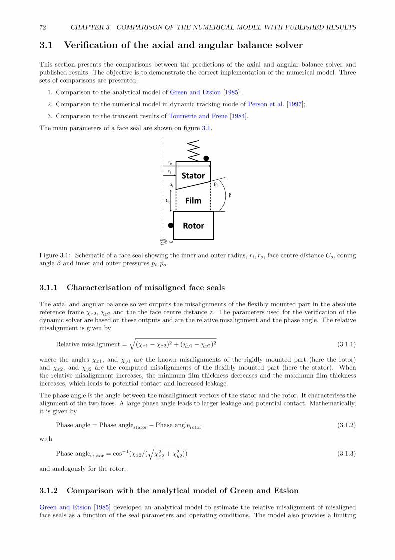
72 CHAPTER 3. COMPARISON OF THE NUMERICAL MODEL WITH PUBLISHED RESULTS
3.1 Verification of the axial and angular balance solver
This section presents the comparisons between the predictions of the axial and angular balance solver andpublished results. The objective is to demonstrate the correct implementation of the numerical model. Threesets of comparisons are presented:
1. Comparison to the analytical model of Green and Etsion [1985];
2. Comparison to the numerical model in dynamic tracking mode of Person et al. [1997];
3. Comparison to the transient results of Tournerie and Frene [1984].
The main parameters of a face seal are shown on figure 3.1.
Film
Stator
Rotor
ri
ro
Co
β
pi po
ω
Figure 3.1: Schematic of a face seal showing the inner and outer radius, ri, ro, face centre distance Co, coningangle β and inner and outer pressures pi, po.
3.1.1 Characterisation of misaligned face seals
The axial and angular balance solver outputs the misalignments of the flexibly mounted part in the absolutereference frame χx2, χy2 and the the face centre distance z. The parameters used for the verification of thedynamic solver are based on these outputs and are the relative misalignment and the phase angle. The relativemisalignment is given by
Relative misalignment =√
(χx1 − χx2)2 + (χy1 − χy2)2 (3.1.1)
where the angles χx1, and χy1 are the known misalignments of the rigidly mounted part (here the rotor)and χx2, and χy2 are the computed misalignments of the flexibly mounted part (here the stator). Whenthe relative misalignment increases, the minimum film thickness decreases and the maximum film thicknessincreases, which leads to potential contact and increased leakage.
The phase angle is the angle between the misalignment vectors of the stator and the rotor. It characterises thealignment of the two faces. A large phase angle leads to larger leakage and potential contact. Mathematically,it is given by
Phase angle = Phase anglestator − Phase anglerotor (3.1.2)
with
Phase anglestator = cos−1(χx2/(√χ2x2 + χ2
y2)) (3.1.3)
and analogously for the rotor.
3.1.2 Comparison with the analytical model of Green and Etsion
Green and Etsion [1985] developed an analytical model to estimate the relative misalignment of misalignedface seals as a function of the seal parameters and operating conditions. The model also provides a limiting
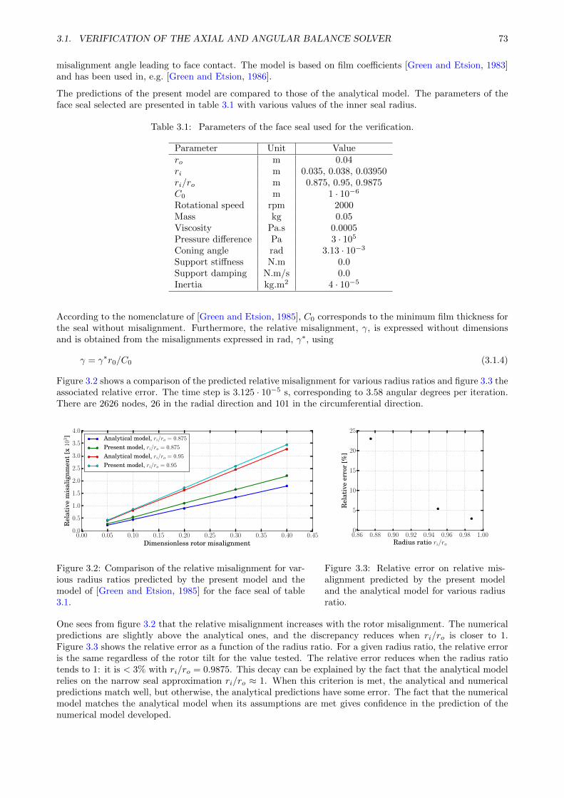
3.1. VERIFICATION OF THE AXIAL AND ANGULAR BALANCE SOLVER 73
misalignment angle leading to face contact. The model is based on film coefficients [Green and Etsion, 1983]and has been used in, e.g. [Green and Etsion, 1986].
The predictions of the present model are compared to those of the analytical model. The parameters of theface seal selected are presented in table 3.1 with various values of the inner seal radius.
Table 3.1: Parameters of the face seal used for the verification.
Parameter Unit Valuero m 0.04ri m 0.035, 0.038, 0.03950ri/ro m 0.875, 0.95, 0.9875C0 m 1 · 10−6
Rotational speed rpm 2000Mass kg 0.05Viscosity Pa.s 0.0005Pressure difference Pa 3 · 105
Coning angle rad 3.13 · 10−3
Support stiffness N.m 0.0Support damping N.m/s 0.0Inertia kg.m2 4 · 10−5
According to the nomenclature of [Green and Etsion, 1985], C0 corresponds to the minimum film thickness forthe seal without misalignment. Furthermore, the relative misalignment, γ, is expressed without dimensionsand is obtained from the misalignments expressed in rad, γ∗, using
γ = γ∗r0/C0 (3.1.4)
Figure 3.2 shows a comparison of the predicted relative misalignment for various radius ratios and figure 3.3 theassociated relative error. The time step is 3.125 · 10−5 s, corresponding to 3.58 angular degrees per iteration.There are 2626 nodes, 26 in the radial direction and 101 in the circumferential direction.
0.00 0.05 0.10 0.15 0.20 0.25 0.30 0.35 0.40 0.45Dimensionless rotor misalignment
0.0
0.5
1.0
1.5
2.0
2.5
3.0
3.5
4.0
Rel
ativ
em
isal
ignm
ent
[x10
3] Analytical model, ri/ro = 0.875
Present model, ri/ro = 0.875
Analytical model, ri/ro = 0.95
Present model, ri/ro = 0.95
Figure 3.2: Comparison of the relative misalignment for var-ious radius ratios predicted by the present model and themodel of [Green and Etsion, 1985] for the face seal of table3.1.
0.86 0.88 0.90 0.92 0.94 0.96 0.98 1.00Radius ratio ri/ro
0
5
10
15
20
25
Rel
ativ
eer
ror
[%]
Figure 3.3: Relative error on relative mis-alignment predicted by the present modeland the analytical model for various radiusratio.
One sees from figure 3.2 that the relative misalignment increases with the rotor misalignment. The numericalpredictions are slightly above the analytical ones, and the discrepancy reduces when ri/ro is closer to 1.Figure 3.3 shows the relative error as a function of the radius ratio. For a given radius ratio, the relative erroris the same regardless of the rotor tilt for the value tested. The relative error reduces when the radius ratiotends to 1: it is < 3% with ri/ro = 0.9875. This decay can be explained by the fact that the analytical modelrelies on the narrow seal approximation ri/ro ≈ 1. When this criterion is met, the analytical and numericalpredictions match well, but otherwise, the analytical predictions have some error. The fact that the numericalmodel matches the analytical model when its assumptions are met gives confidence in the prediction of thenumerical model developed.
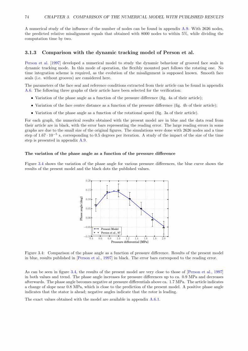
74 CHAPTER 3. COMPARISON OF THE NUMERICAL MODEL WITH PUBLISHED RESULTS
A numerical study of the influence of the number of nodes can be found in appendix A.9. With 2626 nodes,the predicted relative misalignment equals that obtained with 8000 nodes to within 5%, while dividing thecomputation time by two.
3.1.3 Comparison with the dynamic tracking model of Person et al.
Person et al. [1997] developed a numerical model to study the dynamic behaviour of grooved face seals indynamic tracking mode. In this mode of operation, the flexibly mounted part follows the rotating one. Notime integration scheme is required, as the evolution of the misalignment is supposed known. Smooth faceseals (i.e. without grooves) are considered here.
The parameters of the face seal and reference conditions extracted from their article can be found in appendixA.6. The following three graphs of their article have been selected for the verification:
Variation of the phase angle as a function of the pressure difference (fig. 4a of their article);
Variation of the face centre distance as a function of the pressure difference (fig. 4b of their article);
Variation of the phase angle as a function of the rotational speed (fig. 3a of their article).
For each graph, the numerical results obtained with the present model are in blue and the data read fromtheir article are in black, with the error bars representing the reading error. The large reading errors in somegraphs are due to the small size of the original figures. The simulations were done with 2626 nodes and a timestep of 1.67 · 10−5 s, corresponding to 0.5 degrees per iteration. A study of the impact of the size of the timestep is presented in appendix A.9.
The variation of the phase angle as a function of the pressure difference
Figure 3.4 shows the variation of the phase angle for various pressure differences, the blue curve shows theresults of the present model and the black dots the published values.
0.4 0.6 0.8 1.0 1.2 1.4 1.6 1.8 2.0Pressure differential [MPa]
−0.10
−0.05
0.00
0.05
0.10
0.15
0.20
Pha
sean
gle
[deg
]
Present ModelPerson et al., 97
Figure 3.4: Comparison of the phase angle as a function of pressure difference. Results of the present modelin blue, results published in [Person et al., 1997] in black. The error bars correspond to the reading error.
As can be seen in figure 3.4, the results of the present model are very close to those of [Person et al., 1997]in both values and trend. The phase angle increases for pressure differences up to ca. 0.9 MPa and decreasesafterwards. The phase angle becomes negative at pressure differentials above ca. 1.7 MPa. The article indicatesa change of slope near 0.8 MPa, which is close to the prediction of the present model. A positive phase angleindicates that the stator is ahead; negative angles indicate that the rotor is leading.
The exact values obtained with the model are available in appendix A.6.1.
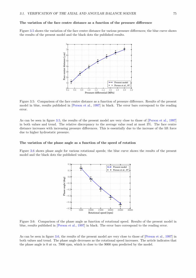
3.1. VERIFICATION OF THE AXIAL AND ANGULAR BALANCE SOLVER 75
The variation of the face centre distance as a function of the pressure difference
Figure 3.5 shows the variation of the face centre distance for various pressure differences; the blue curve showsthe results of the present model and the black dots the published results.
0.4 0.6 0.8 1.0 1.2 1.4 1.6 1.8 2.0 2.2Pressure differential [MPa]
0
1
2
3
4
5
6
7
8
Face
cent
erdi
stan
ce[µ
m]
Present modelPerson et al., 97
Figure 3.5: Comparison of the face centre distance as a function of pressure difference. Results of the presentmodel in blue, results published in [Person et al., 1997] in black. The error bars correspond to the readingerror.
As can be seen in figure 3.5, the results of the present model are very close to those of [Person et al., 1997]in both values and trend. The relative discrepancy to the average value read at most 3%. The face centredistance increases with increasing pressure differences. This is essentially due to the increase of the lift forcedue to higher hydrostatic pressure.
The variation of the phase angle as a function of the speed of rotation
Figure 3.6 shows phase angle for various rotational speeds; the blue curve shows the results of the presentmodel and the black dots the published values.
0 5000 10000 15000 20000 25000 30000Rotational speed [rpm]
−0.5
−0.4
−0.3
−0.2
−0.1
0.0
0.1
0.2
Pha
sean
gle
[deg
]
Present modelPerson et al., 97
Figure 3.6: Comparison of the phase angle as function of rotational speed. Results of the present model inblue, results published in [Person et al., 1997] in black. The error bars correspond to the reading error.
As can be seen in figure 3.6, the results of the present model are very close to those of [Person et al., 1997] inboth values and trend. The phase angle decreases as the rotational speed increases. The article indicates thatthe phase angle is 0 at ca. 7000 rpm, which is close to the 9000 rpm predicted by the model.
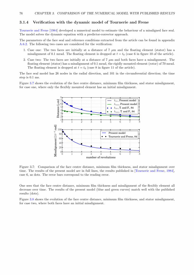
76 CHAPTER 3. COMPARISON OF THE NUMERICAL MODEL WITH PUBLISHED RESULTS
3.1.4 Verification with the dynamic model of Tournerie and Frene
Tournerie and Frene [1984] developed a numerical model to estimate the behaviour of a misaligned face seal.The model solves the dynamic equation with a predictor-corrector approach.
The parameters of the face seal and reference conditions extracted from the article can be found in appendixA.6.2. The following two cases are considered for the verification:
1. Case one: The two faces are initially at a distance of 7 µm and the floating element (stator) has amisalignment of 0.1 mrad. The floating element is dropped at t = t0 (case 6 in figure 10 of the article).
2. Case two: The two faces are initially at a distance of 7 µm and both faces have a misalignment. Thefloating element (stator) has a misalignment of 0.1 mrad, the rigidly mounted element (rotor) of 70 mrad.The floating element is dropped at t = t0 (case 8 in figure 11 of the article).
The face seal model has 26 nodes in the radial direction, and 101 in the circumferential direction; the timestep is 0.1 ms.
Figure 3.7 shows the evolution of the face centre distance, minimum film thickness, and stator misalignment,for case one, where only the flexibly mounted element has an initial misalignment.
0 1 2 3 4 5 6 7 812345678
Dis
tanc
e[µ
m] hctr, Present model
hmin, Present modelhctr, T. and F., 84hmin, T. and F., 84
0 1 2 3 4 5 6 7 8number of revolutions
0
20
40
60
80
100
Mis
alig
nmen
t[1
0−6
rad]
Present modelTournerie and Frene, 84
Figure 3.7: Comparison of the face centre distance, minimum film thickness, and stator misalignment overtime. The results of the present model are in full lines, the results published in [Tournerie and Frene, 1984],case 6, as dots. The error bars correspond to the reading error.
One sees that the face centre distance, minimum film thickness and misalignment of the flexibly element alldecrease over time. The results of the present model (blue and green curves) match well with the publishedresults (dots).
Figure 3.8 shows the evolution of the face centre distance, minimum film thickness, and stator misalignment,for case two, where both faces have an initial misalignment.
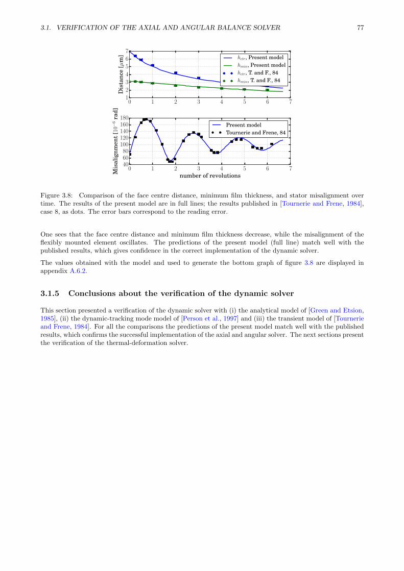
3.1. VERIFICATION OF THE AXIAL AND ANGULAR BALANCE SOLVER 77
0 1 2 3 4 5 6 71
2
3
4
5
6
7
Dis
tanc
e[µ
m] hctr, Present model
hmin, Present modelhctr, T. and F., 84hmin, T. and F., 84
0 1 2 3 4 5 6 7number of revolutions
406080
100120140160180
Mis
alig
nmen
t[1
0−6
rad]
Present modelTournerie and Frene, 84
Figure 3.8: Comparison of the face centre distance, minimum film thickness, and stator misalignment overtime. The results of the present model are in full lines; the results published in [Tournerie and Frene, 1984],case 8, as dots. The error bars correspond to the reading error.
One sees that the face centre distance and minimum film thickness decrease, while the misalignment of theflexibly mounted element oscillates. The predictions of the present model (full line) match well with thepublished results, which gives confidence in the correct implementation of the dynamic solver.
The values obtained with the model and used to generate the bottom graph of figure 3.8 are displayed inappendix A.6.2.
3.1.5 Conclusions about the verification of the dynamic solver
This section presented a verification of the dynamic solver with (i) the analytical model of [Green and Etsion,1985], (ii) the dynamic-tracking mode model of [Person et al., 1997] and (iii) the transient model of [Tournerieand Frene, 1984]. For all the comparisons the predictions of the present model match well with the publishedresults, which confirms the successful implementation of the axial and angular solver. The next sections presentthe verification of the thermal-deformation solver.
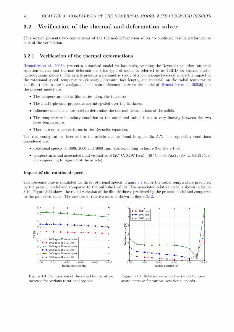
78 CHAPTER 3. COMPARISON OF THE NUMERICAL MODEL WITH PUBLISHED RESULTS
3.2 Verification of the thermal and deformation solver
This section presents two comparisons of the thermal-deformation solver to published results performed aspart of the verification.
3.2.1 Verification of the thermal deformations
Brunetiere et al. [2003b] present a numerical model for face seals, coupling the Reynolds equation, an axialequation solver, and thermal deformations (this type of model is referred to as TEHD for thermo-elasto-hydrodynamic model). The article presents a parametric study of a low leakage face seal where the impact ofthe rotational speed, temperature (viscosity), pressure, face length, and material, on the radial temperatureand film thickness are investigated. The main differences between the model of [Brunetiere et al., 2003b] andthe present model are:
The temperature of the film varies along the thickness.
The fluid’s physical properties are integrated over the thickness.
Influence coefficients are used to determine the thermal deformations of the solids.
The temperature boundary condition at the outer seal radius is set to vary linearly between the twofaces temperature.
There are no transient terms in the Reynolds equation.
The seal configuration described in the article can be found in appendix A.7. The operating conditionsconsidered are:
rotational speeds of 1000, 2000 and 5000 rpm (corresponding to figure 3 of the article)
temperatures and associated fluid viscosities of (20 C, 0.197 Pa.s); (40 C, 0.08 Pa.s) ; (80 C, 0.013 Pa.s)(corresponding to figure 4 of the article)
Impact of the rotational speed
The reference case is simulated for three rotational speeds. Figure 3.9 shows the radial temperature predictedby the present model and compared to the published values. The associated relative error is shown in figure3.10. Figure 3.11 shows the radial variation of the film thickness predicted by the present model and comparedto the published value. The associated relative error is shown in figure 3.12.
0.040 0.041 0.042 0.043 0.044 0.045Radial position [m]
0
10
20
30
40
50
60
70
80
∆T
[K]
1000 rpm, Present model1000 rpm, B. et al., 032000 rpm, Present model2000 rpm, B. et al., 035000 rpm, Present model5000 rpm, B. et al., 03
Figure 3.9: Comparison of the radial temperatureincrease for various rotational speeds.
0.040 0.041 0.042 0.043 0.044 0.045Radial position [m]
0
1
2
3
4
5
6
Rel
ativ
eer
ror
[%]
1000 rpm2000 rpm5000 rpm
Figure 3.10: Relative error on the radial temper-ature increase for various rotational speeds.
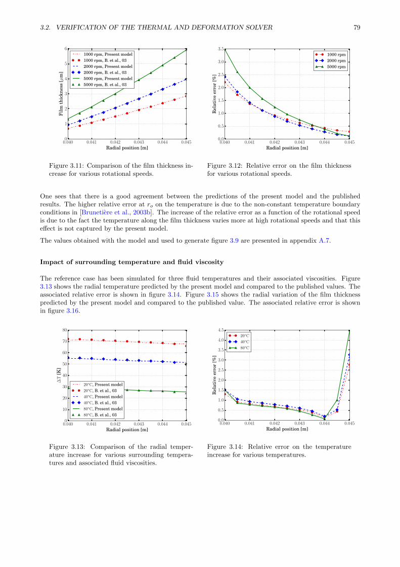
3.2. VERIFICATION OF THE THERMAL AND DEFORMATION SOLVER 79
0.040 0.041 0.042 0.043 0.044 0.045Radial position [m]
0
1
2
3
4
5
6
Film
thic
knes
s[µ
m]
1000 rpm, Present model1000 rpm, B. et al., 032000 rpm, Present model2000 rpm, B. et al., 035000 rpm, Present model5000 rpm, B. et al., 03
Figure 3.11: Comparison of the film thickness in-crease for various rotational speeds.
0.040 0.041 0.042 0.043 0.044 0.045Radial position [m]
0.0
0.5
1.0
1.5
2.0
2.5
3.0
3.5
Rel
ativ
eer
ror
[%]
1000 rpm2000 rpm5000 rpm
Figure 3.12: Relative error on the film thicknessfor various rotational speeds.
One sees that there is a good agreement between the predictions of the present model and the publishedresults. The higher relative error at ro on the temperature is due to the non-constant temperature boundaryconditions in [Brunetiere et al., 2003b]. The increase of the relative error as a function of the rotational speedis due to the fact the temperature along the film thickness varies more at high rotational speeds and that thiseffect is not captured by the present model.
The values obtained with the model and used to generate figure 3.9 are presented in appendix A.7.
Impact of surrounding temperature and fluid viscosity
The reference case has been simulated for three fluid temperatures and their associated viscosities. Figure3.13 shows the radial temperature predicted by the present model and compared to the published values. Theassociated relative error is shown in figure 3.14. Figure 3.15 shows the radial variation of the film thicknesspredicted by the present model and compared to the published value. The associated relative error is shownin figure 3.16.
0.040 0.041 0.042 0.043 0.044 0.045Radial position [m]
0
10
20
30
40
50
60
70
80
∆T
[K]
20C, Present model20C, B. et al., 0340C, Present model40C, B. et al., 0380C, Present model80C, B. et al., 03
Figure 3.13: Comparison of the radial temper-ature increase for various surrounding tempera-tures and associated fluid viscosities.
0.040 0.041 0.042 0.043 0.044 0.045Radial position [m]
0.0
0.5
1.0
1.5
2.0
2.5
3.0
3.5
4.0
4.5
Rel
ativ
eer
ror
[%]
20C
40C
80C
Figure 3.14: Relative error on the temperatureincrease for various temperatures.
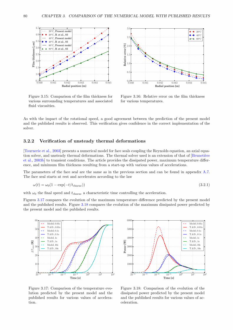
80 CHAPTER 3. COMPARISON OF THE NUMERICAL MODEL WITH PUBLISHED RESULTS
0.040 0.041 0.042 0.043 0.044 0.045Radial position [m]
0.5
1.0
1.5
2.0
2.5
3.0
3.5
4.0
4.5
Film
thic
knes
s[µ
m]
20C, Present model20C, B. et al., 0340C, Present model40C, B. et al., 0380C, Present model80C, B. et al., 03
Figure 3.15: Comparison of the film thickness forvarious surrounding temperatures and associatedfluid viscosities.
0.040 0.041 0.042 0.043 0.044 0.045Radial position [m]
0.0
0.5
1.0
1.5
2.0
2.5
3.0
Rel
ativ
eer
ror
[%]
20C
40C
80C
Figure 3.16: Relative error on the film thicknessfor various temperatures.
As with the impact of the rotational speed, a good agreement between the prediction of the present modeland the published results is observed. This verification gives confidence in the correct implementation of thesolver.
3.2.2 Verification of unsteady thermal deformations
[Tournerie et al., 2003] presents a numerical model for face seals coupling the Reynolds equation, an axial equa-tion solver, and unsteady thermal deformations. The thermal solver used is an extension of that of [Brunetiereet al., 2003b] to transient conditions. The article provides the dissipated power, maximum temperature differ-ence, and minimum film thickness resulting from a start-up with various values of accelerations.
The parameters of the face seal are the same as in the previous section and can be found in appendix A.7.The face seal starts at rest and accelerates according to the law
ω(t) = ω0(1− exp(−t/tcharac)) (3.2.1)
with ω0 the final speed and tcharac a characteristic time controlling the acceleration.
Figures 3.17 compares the evolution of the maximum temperature difference predicted by the present modeland the published results. Figure 3.18 compares the evolution of the maximum dissipated power predicted bythe present model and the published results.
10−4 10−3 10−2 10−1 100 101 102
Time [s]
0
10
20
30
40
50
60
∆T
max
[K]
Model, 0.01s
T.&D., 0.01s
Model, 0.1s
T.&D., 0.1s
Model, 1s
T.&D., 1s
Model, 10s
T.&D., 10s
Figure 3.17: Comparison of the temperature evo-lution predicted by the present model and thepublished results for various values of accelera-tion.
10−4 10−3 10−2 10−1 100 101 102
Time [s]
0
1000
2000
3000
4000
5000
6000
Pow
er[W
]
Model, 0.01s
T.&D., 0.01s
Model, 0.1s
T.&D., 0.1s
Model, 1s
T.&D., 1s
Model, 10s
T.&D., 10s
Figure 3.18: Comparison of the evolution of thedissipated power predicted by the present modeland the published results for various values of ac-celeration.

3.2. VERIFICATION OF THE THERMAL AND DEFORMATION SOLVER 81
One sees that the predictions of the present model match well with the published results, which confirms thecorrect implementation of the transient thermal model.
Note that the model of [Tournerie et al., 2003] considers a steady-state form of the Reynolds equation. Forthe comparison, the transient term in the Reynolds equation of the present model was removed.
3.2.3 Conclusion about the verification of the thermal solver
This section presented a verification of the thermal deformation solver of the face seal model using the articlesof [Brunetiere et al., 2003b] for the steady thermal deformations and [Tournerie et al., 2003] for the unsteadythermal deformation. The predictions of the model match well with the published results which confirmsthe successful implementation of the thermal deformation solver. The verification of the pure mechanicaldeformations was also performed but is not presented here. The next section of this part presents a comparisonof the predictions of the model with the experimental results.
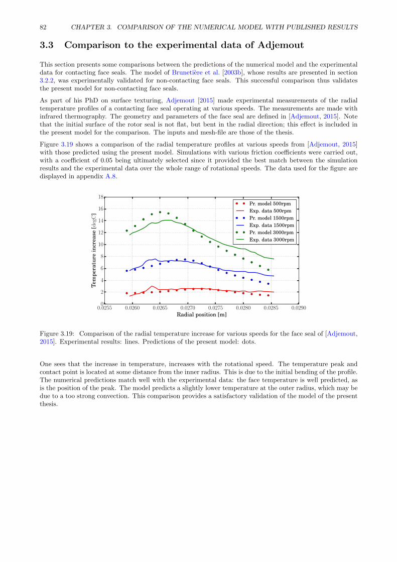
82 CHAPTER 3. COMPARISON OF THE NUMERICAL MODEL WITH PUBLISHED RESULTS
3.3 Comparison to the experimental data of Adjemout
This section presents some comparisons between the predictions of the numerical model and the experimentaldata for contacting face seals. The model of Brunetiere et al. [2003b], whose results are presented in section3.2.2, was experimentally validated for non-contacting face seals. This successful comparison thus validatesthe present model for non-contacting face seals.
As part of his PhD on surface texturing, Adjemout [2015] made experimental measurements of the radialtemperature profiles of a contacting face seal operating at various speeds. The measurements are made withinfrared thermography. The geometry and parameters of the face seal are defined in [Adjemout, 2015]. Notethat the initial surface of the rotor seal is not flat, but bent in the radial direction; this effect is included inthe present model for the comparison. The inputs and mesh-file are those of the thesis.
Figure 3.19 shows a comparison of the radial temperature profiles at various speeds from [Adjemout, 2015]with those predicted using the present model. Simulations with various friction coefficients were carried out,with a coefficient of 0.05 being ultimately selected since it provided the best match between the simulationresults and the experimental data over the whole range of rotational speeds. The data used for the figure aredisplayed in appendix A.8.
0.0255 0.0260 0.0265 0.0270 0.0275 0.0280 0.0285 0.0290Radial position [m]
0
2
4
6
8
10
12
14
16
18
Tem
pera
ture
incr
ease
[deg
C]
Pr. model 500rpmExp. data 500rpmPr. model 1500rpmExp. data 1500rpmPr. model 3000rpmExp. data 3000rpm
Figure 3.19: Comparison of the radial temperature increase for various speeds for the face seal of [Adjemout,2015]. Experimental results: lines. Predictions of the present model: dots.
One sees that the increase in temperature, increases with the rotational speed. The temperature peak andcontact point is located at some distance from the inner radius. This is due to the initial bending of the profile.The numerical predictions match well with the experimental data: the face temperature is well predicted, asis the position of the peak. The model predicts a slightly lower temperature at the outer radius, which may bedue to a too strong convection. This comparison provides a satisfactory validation of the model of the presentthesis.
3.4. SUMMARY OF THE NUMERICAL MODEL VERIFICATION AND VALIDATION 83
3.4 Summary of the numerical model verification and validation
This section presented various comparisons verifying and validating the face seal model developed for thepresent thesis. In particular, the following verifications have been presented:
Verification of the dynamic solver by comparison with the analytical model of [Green and Etsion, 1985];
Verification of the dynamic solver by comparing it to the dynamic-tracking model of [Person et al., 1997];
Verification of the dynamic solver by comparing it to the transient model of [Tournerie and Frene, 1984];
Verification of the thermal and thermal deformation solver by comparison with [Brunetiere et al., 2003b];
Verification of the transient thermal and thermal deformation solver by comparison them with [Tournerieet al., 2003].
The verifications provided satisfactory results, which confirms the correct implementation of the model. Thevalidation was made by successfully comparing the predictions of the present model with the experimentaldata of [Adjemout, 2015]. The comparison with this representative experimental data is satisfactory, whichgives confidence in the ability of the model to predict the performance of face seals. The studies performedwith the model are presented in chapter 5.

84 CHAPTER 3. COMPARISON OF THE NUMERICAL MODEL WITH PUBLISHED RESULTS
Chapter 4
Experimental test setup
The objective of this chapter is to present the industrial test setup as well as the instrumentation and testmethods developed. The test results are part of the numerical and experimental studies and will be presentedand analysed in chapter 5 of this thesis.
The overall project includes industrial motivations. The setup is an industrial apparatus designed to reproducesevere operating conditions - pressure, temperature, and pressure inversions - and to investigate their effectson the performance of a face seal.
Contents4.1 System description . . . . . . . . . . . . . . . . . . . . . . . . . . . . . . . . . . . . 86
4.1.1 Industrial test setup . . . . . . . . . . . . . . . . . . . . . . . . . . . . . . . . . . . . 86
4.1.2 Face seal holder . . . . . . . . . . . . . . . . . . . . . . . . . . . . . . . . . . . . . . . 86
4.1.3 Face seal . . . . . . . . . . . . . . . . . . . . . . . . . . . . . . . . . . . . . . . . . . 87
4.2 Instrumentation . . . . . . . . . . . . . . . . . . . . . . . . . . . . . . . . . . . . . . 89
4.2.1 Measure of the volume of fluid in the reservoir . . . . . . . . . . . . . . . . . . . . . 89
4.2.2 Measurements of the inner and outer pressures of the face seal . . . . . . . . . . . . 90
4.2.3 Measurement of water ingression . . . . . . . . . . . . . . . . . . . . . . . . . . . . . 90
4.3 Setup characterisation . . . . . . . . . . . . . . . . . . . . . . . . . . . . . . . . . . 92
4.3.1 Emergency shut-down . . . . . . . . . . . . . . . . . . . . . . . . . . . . . . . . . . . 92
4.3.2 Temperature . . . . . . . . . . . . . . . . . . . . . . . . . . . . . . . . . . . . . . . . 92
4.3.3 Pressure . . . . . . . . . . . . . . . . . . . . . . . . . . . . . . . . . . . . . . . . . . . 92
4.3.4 Rotational speed . . . . . . . . . . . . . . . . . . . . . . . . . . . . . . . . . . . . . . 92
4.3.5 Operating test conditions . . . . . . . . . . . . . . . . . . . . . . . . . . . . . . . . . 93
4.3.6 Face seal pressure difference . . . . . . . . . . . . . . . . . . . . . . . . . . . . . . . . 93
4.4 Test procedure . . . . . . . . . . . . . . . . . . . . . . . . . . . . . . . . . . . . . . . 97
4.5 Summary of the experimental test setup . . . . . . . . . . . . . . . . . . . . . . . 98
85
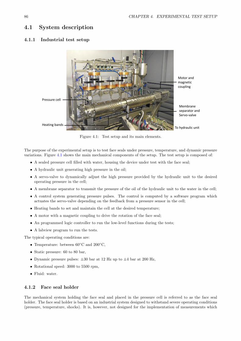
86 CHAPTER 4. EXPERIMENTAL TEST SETUP
4.1 System description
4.1.1 Industrial test setup
Pressure cell
Membrane separator andServo-valve
To hydraulic unit
Motor and magnetic coupling
Heating bands
Figure 4.1: Test setup and its main elements.
The purpose of the experimental setup is to test face seals under pressure, temperature, and dynamic pressurevariations. Figure 4.1 shows the main mechanical components of the setup. The test setup is composed of:
A sealed pressure cell filled with water, housing the device under test with the face seal;
A hydraulic unit generating high pressure in the oil;
A servo-valve to dynamically adjust the high pressure provided by the hydraulic unit to the desiredoperating pressure in the cell;
A membrane separator to transmit the pressure of the oil of the hydraulic unit to the water in the cell;
A control system generating pressure pulses. The control is computed by a software program whichactuates the servo-valve depending on the feedback from a pressure sensor in the cell;
Heating bands to set and maintain the cell at the desired temperature;
A motor with a magnetic coupling to drive the rotation of the face seal;
An programmed logic controller to run the low-level functions during the tests;
A labview program to run the tests.
The typical operating conditions are:
Temperature: between 60C and 200C,
Static pressure: 60 to 80 bar,
Dynamic pressure pulses: ±30 bar at 12 Hz up to ±4 bar at 200 Hz,
Rotational speed: 3000 to 5500 rpm,
Fluid: water.
4.1.2 Face seal holder
The mechanical system holding the face seal and placed in the pressure cell is referred to as the face sealholder. The face seal holder is based on an industrial system designed to withstand severe operating conditions(pressure, temperature, shocks). It is, however, not designed for the implementation of measurements which
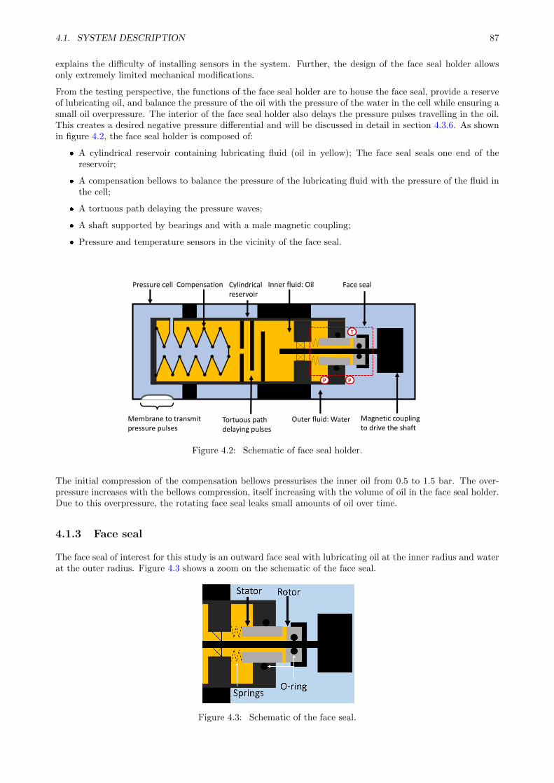
4.1. SYSTEM DESCRIPTION 87
explains the difficulty of installing sensors in the system. Further, the design of the face seal holder allowsonly extremely limited mechanical modifications.
From the testing perspective, the functions of the face seal holder are to house the face seal, provide a reserveof lubricating oil, and balance the pressure of the oil with the pressure of the water in the cell while ensuring asmall oil overpressure. The interior of the face seal holder also delays the pressure pulses travelling in the oil.This creates a desired negative pressure differential and will be discussed in detail in section 4.3.6. As shownin figure 4.2, the face seal holder is composed of:
A cylindrical reservoir containing lubricating fluid (oil in yellow); The face seal seals one end of thereservoir;
A compensation bellows to balance the pressure of the lubricating fluid with the pressure of the fluid inthe cell;
A tortuous path delaying the pressure waves;
A shaft supported by bearings and with a male magnetic coupling;
Pressure and temperature sensors in the vicinity of the face seal.
P P
T
Compensation Inner fluid: Oil Face seal
Membrane to transmit pressure pulses
Outer fluid: Water Magnetic coupling to drive the shaft
Tortuous path delaying pulses
Cylindrical reservoir
Pressure cell
Figure 4.2: Schematic of face seal holder.
The initial compression of the compensation bellows pressurises the inner oil from 0.5 to 1.5 bar. The over-pressure increases with the bellows compression, itself increasing with the volume of oil in the face seal holder.Due to this overpressure, the rotating face seal leaks small amounts of oil over time.
4.1.3 Face seal
The face seal of interest for this study is an outward face seal with lubricating oil at the inner radius and waterat the outer radius. Figure 4.3 shows a zoom on the schematic of the face seal.
Schlu
mb
erger Co
nfid
ential
Figure 4.3: Schematic of the face seal.

88 CHAPTER 4. EXPERIMENTAL TEST SETUP
The stator is linked to the face seal holder by springs and an O-ring. The O-ring acts as a semi-dynamic sealbetween the stator and the face seal holder. The springs press the stator against the rotor. The sides of thestator facing the housing have flats (not represented) which prevent its rotation and limit its swiveling. Thestator part is 16 mm long and the contact area has an inner radius of 11.4 mm and outer radius of 14.3 mm.The rotor is 9 mm long and its contact area has the same diameters as the stator. The rotor has an O-ringat the inner radius acting as a seal between the shaft and rotor. The rotor also has flats facing its holderto transmit the rotation of the shaft. The rotor is blocked axially in the direction opposite to the stator(translation from left to right according to figure 4.3 is prevented).
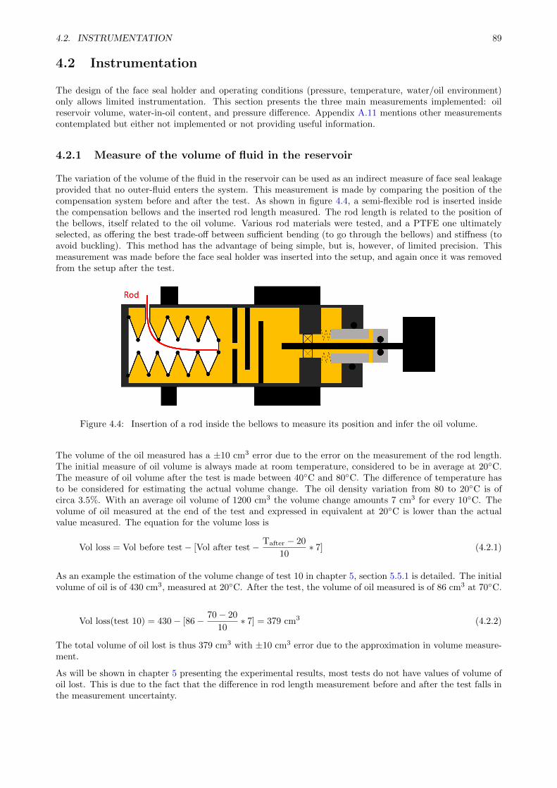
4.2. INSTRUMENTATION 89
4.2 Instrumentation
The design of the face seal holder and operating conditions (pressure, temperature, water/oil environment)only allows limited instrumentation. This section presents the three main measurements implemented: oilreservoir volume, water-in-oil content, and pressure difference. Appendix A.11 mentions other measurementscontemplated but either not implemented or not providing useful information.
4.2.1 Measure of the volume of fluid in the reservoir
The variation of the volume of the fluid in the reservoir can be used as an indirect measure of face seal leakageprovided that no outer-fluid enters the system. This measurement is made by comparing the position of thecompensation system before and after the test. As shown in figure 4.4, a semi-flexible rod is inserted insidethe compensation bellows and the inserted rod length measured. The rod length is related to the position ofthe bellows, itself related to the oil volume. Various rod materials were tested, and a PTFE one ultimatelyselected, as offering the best trade-off between sufficient bending (to go through the bellows) and stiffness (toavoid buckling). This method has the advantage of being simple, but is, however, of limited precision. Thismeasurement was made before the face seal holder was inserted into the setup, and again once it was removedfrom the setup after the test.
Figure 4.4: Insertion of a rod inside the bellows to measure its position and infer the oil volume.
The volume of the oil measured has a ±10 cm3 error due to the error on the measurement of the rod length.The initial measure of oil volume is always made at room temperature, considered to be in average at 20C.The measure of oil volume after the test is made between 40C and 80C. The difference of temperature hasto be considered for estimating the actual volume change. The oil density variation from 80 to 20C is ofcirca 3.5%. With an average oil volume of 1200 cm3 the volume change amounts 7 cm3 for every 10C. Thevolume of oil measured at the end of the test and expressed in equivalent at 20C is lower than the actualvalue measured. The equation for the volume loss is
Vol loss = Vol before test− [Vol after test− Tafter − 20
10∗ 7] (4.2.1)
As an example the estimation of the volume change of test 10 in chapter 5, section 5.5.1 is detailed. The initialvolume of oil is of 430 cm3, measured at 20C. After the test, the volume of oil measured is of 86 cm3 at 70C.
Vol loss(test 10) = 430− [86− 70− 20
10∗ 7] = 379 cm3 (4.2.2)
The total volume of oil lost is thus 379 cm3 with ±10 cm3 error due to the approximation in volume measure-ment.
As will be shown in chapter 5 presenting the experimental results, most tests do not have values of volume ofoil lost. This is due to the fact that the difference in rod length measurement before and after the test falls inthe measurement uncertainty.
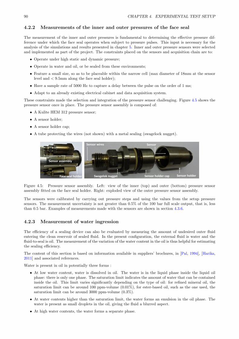
90 CHAPTER 4. EXPERIMENTAL TEST SETUP
4.2.2 Measurements of the inner and outer pressures of the face seal
The measurement of the inner and outer pressures is fundamental to determining the effective pressure dif-ference under which the face seal operates when subject to pressure pulses. This input is necessary for theanalysis of the simulations and results presented in chapter 5. Inner and outer pressure sensors were selectedand implemented as part of the project. The constraints placed on the sensors and acquisition chain are to:
Operate under high static and dynamic pressure;
Operate in water and oil, or be sealed from these environments;
Feature a small size, so as to be placeable within the narrow cell (max diameter of 18mm at the sensorlevel and < 9.5mm along the face seal holder);
Have a sample rate of 5000 Hz to capture a delay between the pulse on the order of 1 ms;
Adapt to an already existing electrical cabinet and data acquisition system.
These constraints made the selection and integration of the pressure sensor challenging. Figure 4.5 shows thepressure sensor once in place. The pressure sensor assembly is composed of:
A Kulite HEM 312 pressure sensor;
A sensor holder;
A sensor holder cap;
A tube protecting the wires (not shown) with a metal sealing (swagelock nugget).
Sensor holderSensor holder capSwagelok nugget
Sensor wires Sensor
Face seal holder
Sensor assembly
Figure 4.5: Pressure sensor assembly. Left: view of the inner (top) and outer (bottom) pressure sensorassembly fitted on the face seal holder. Right: exploded view of the outer pressure sensor assembly.
The sensors were calibrated by carrying out pressure steps and using the values from the setup pressuresensors. The measurement uncertainty is not greater than 0.5% of the 100 bar full scale output, that is, lessthan 0.5 bar. Examples of measurements made with the sensors are shown in section 4.3.6.
4.2.3 Measurement of water ingression
The efficiency of a sealing device can also be evaluated by measuring the amount of undesired outer fluidentering the clean reservoir of sealed fluid. In the present configuration, the external fluid is water and thefluid-to-seal is oil. The measurement of the variation of the water content in the oil is thus helpful for estimatingthe sealing efficiency.
The content of this section is based on information available in suppliers’ brochures, in [Pal, 1994], [Harika,2011] and associated references.
Water is present in oil in potentially three forms :
At low water content, water is dissolved in oil. The water is in the liquid phase inside the liquid oilphase: there is only one phase. The saturation limit indicates the amount of water that can be containedinside the oil. This limit varies significantly depending on the type of oil: for refined mineral oil, thesaturation limit can be around 100 ppm-volume (0.01%), for ester-based oil, such as the one used, thesaturation limit can be around 3000 ppm-volume (0.3%).
At water contents higher than the saturation limit, the water forms an emulsion in the oil phase. Thewater is present as small droplets in the oil, giving the fluid a blurred aspect.
At high water contents, the water forms a separate phase.
4.2. INSTRUMENTATION 91
Measurement device
There are a variety of measurement devices based on different measurement principles, of which an overviewcan be found in [Pal, 1994]. As part of the present project, it was desired to have a measurement device thatcould be readily implemented. Three of the measurement principles considered are presented below as well asthe method selected for the tests.
In-line capacitive measurement method
Measurement of water-in-oil content using a capacitive measurement (measurement of the dielectric constant)is based on the fact that water has a much higher capacitance than oil. The measurement of the capacitance canbe related to the amount of water in the oil solution [Pal, 1994]. An in-line capacitive sensor was considered,but not implemented because of the absence of a commercially available sensor which can withstand thepressures and temperatures and be fit in the system.
Off-line methods
Calcium hydride test
The calcium hydride test is an indirect method which determines the water content through a measurementof the pressure following a reaction transforming water in dihydrogene:
CaH2 + 2H2O→ Ca(OH)2 + 2H2 (4.2.3)
In a sealed cell, the reagent CaH2 reacts with the water H2O of the oil sample of known volume to form a solidCa(OH)2 while releasing H2 gas. The increase of pressure is measured and translated into the quantity of H2Oand subsequently the amount of water in the oil sample. A device of this type with reagents was purchasedand used to obtain an on-site approximate measurement of the water-in-oil content. The advantage of thisapparatus is that it is able to obtain an estimate of the water content directly at the end of the test and thusallows adapting the test conditions for the next test on the same day.
Karl Fisher titration
The Karl Fisher titration method measures all water with a high precision [Standard-NFISO6296, 2001]. Thisapparatus is, however, expensive and usually only available in laboratories. Measurement of the water contentusing the Karl Fisher method was carried out by an external lab to complement the on-site measurementsdone with the calcium hydride test.
Sampling procedure
The determination of the increase in the water-in-oil content is based on the measurement of the water-in-oilcontent before and after a test.
After each test, all the oil is drained from the face seal holder and collected in a container. The collectedoil is stirred and a sample is taken and used for the water content analysis. It is critical to stir the collectedoil to obtain a representative sample. If the oil is not stirred, the water content is higher at the bottomof the container and lower at the top. The representativeness of the sample obtained with this process wasvalidated by measuring the water-in-oil content of several samples. Note that it is not possible to apply thesame procedure for collecting a sample before the test, as this would require emptying the whole system (whichhas to be filled for the test). The sample used for measuring the water content before the test was insteadcollected at the end of the filling process in the outlet pipe connected to the face seal holder. There maybe a difference between the amount of water-in-oil truly present in the system before the test and the valuemeasured. The water-in-oil content of a just-opened can of oil is 0.08%. If the oil stays under vacuum in thepump filling system, the water-in-oil content drops to below 0.02% (the minimum value measurable by thecalcium hydride test at our disposal). The amount of oil in the reservoir of the face seal holder is comprisedbetween 1000 to 1350 cm3, depending on the test. As an example, a measurement of 0.08% of water-in-oilobtained on a representative sample indicates a total of about 1 cm3 water in the whole system.
92 CHAPTER 4. EXPERIMENTAL TEST SETUP
4.3 Setup characterisation
At the start of the project, the test setup had not been validated and it was unclear whether the setup couldoperate according to the functional specifications (pressure, temperature, rotational speed, test duration) andwhether the pressure pulses would lead to pressure inversions at the face seal level. This section presents thesafe operating envelope determined during the first year and one-half of the project, and the measurement ofthe pressure difference.
4.3.1 Emergency shut-down
An emergency shut-down leads to an instantaneous loss of pressure (and vaporization if the temperatureis greater than one hundred degrees Celsius) and subsequent membrane perforation and/or breaking of thecompensation bellows. Due to the time and cost of repairs as well as non-productive time induced, a strongemphasis was placed on avoiding emergency shut-downs. There are two main causes for an emergency shut-down: (i) discrepancy between the pressure measured in the cell and the pressure command (with 15 barcompliance) and (ii) divergence of the optical sensors measuring the position of the membrane in the membraneseparator located between the cell and hydraulic unit. The first cause happens when
the test temperature becomes too high (> 120C), as the pressure sensors do not compensate for atemperature change and start diverging.
The setup has a sealing fault. As a result of the loss of fluid, the membrane of the separator is makingcontact on one side and thus is no longer able to adjust the pressure.
Regarding the second cause, the position of the membrane in the membrane separator is measured using anoptical sensor located in membrane oil. The membranes are slightly permeable and let some water from thecell go through the membrane oil. This water pollutes the oil and leads to an erroneous reading by the opticalsensor.
The first issue is circumvented by limiting the test temperature to 120C. The second issue is remedied bychecking the system’s integrity and performing frequent maintenance. The last issue is remedied by changingthe membrane oil every 150 hours of test or when deemed too polluted.
4.3.2 Temperature
The test temperature is limited to 120C due to the fact that at higher temperatures, the pressure sensorreadings would diverge. Operating above this limit leads to erroneous pressure feedback followed by anemergency shut-down due to a discrepancy between the command and measured pressure. It was decided tooperate at 80C to avoid this operational issue. Note that this value is an average of the water temperature;depending on the thermo-couple position the temperature can be from 75C to 85C.
4.3.3 Pressure
Pressure can be generated without any particular issue. The maximum operating threshold was fixed to 100bar static pressure. In static operation, the pressure command is achieved at ±0.1 bar.
4.3.4 Rotational speed
The rotating magnetic field generates eddy currents in the bell closing the cell and located between the magneticcouplings. These currents lead to extreme heating. To avoid overheating, the speed must not exceed 3500 rpmif the motor is operating continuously. Short time rotations at 5500 rpm are possible, as well as accelerationsup to 1000 rpm per second. The speed command is met at ±2%.
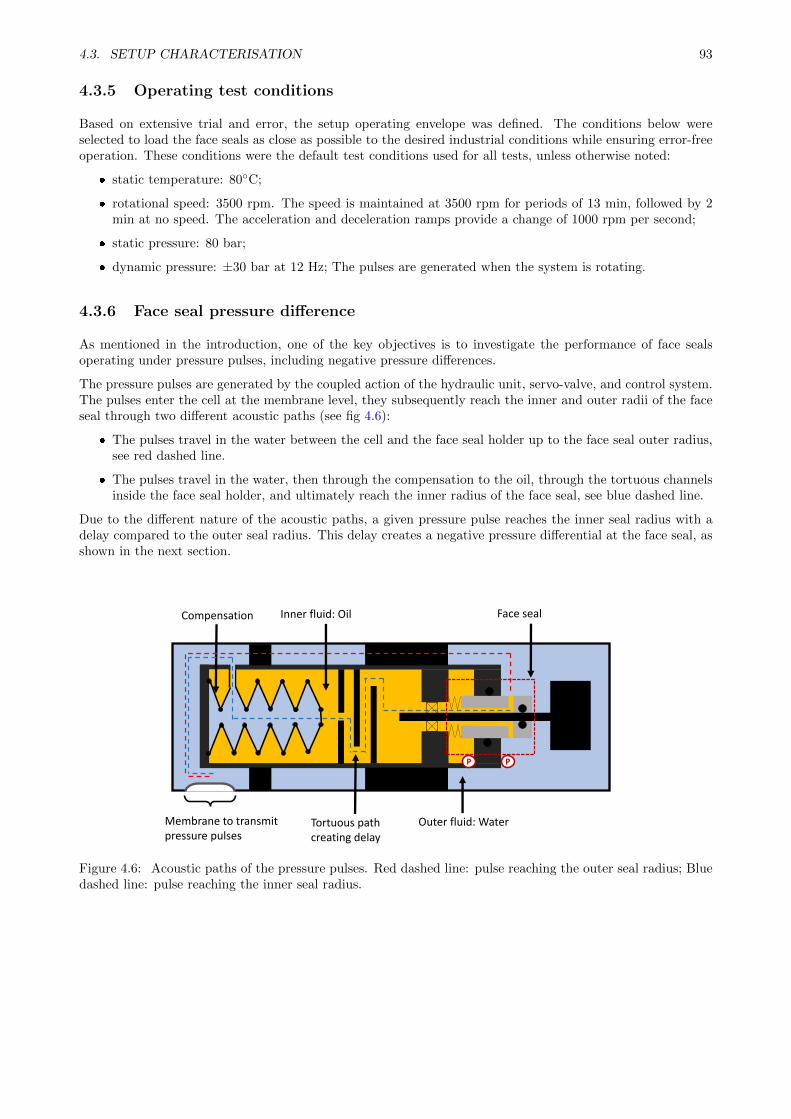
4.3. SETUP CHARACTERISATION 93
4.3.5 Operating test conditions
Based on extensive trial and error, the setup operating envelope was defined. The conditions below wereselected to load the face seals as close as possible to the desired industrial conditions while ensuring error-freeoperation. These conditions were the default test conditions used for all tests, unless otherwise noted:
static temperature: 80C;
rotational speed: 3500 rpm. The speed is maintained at 3500 rpm for periods of 13 min, followed by 2min at no speed. The acceleration and deceleration ramps provide a change of 1000 rpm per second;
static pressure: 80 bar;
dynamic pressure: ±30 bar at 12 Hz; The pulses are generated when the system is rotating.
4.3.6 Face seal pressure difference
As mentioned in the introduction, one of the key objectives is to investigate the performance of face sealsoperating under pressure pulses, including negative pressure differences.
The pressure pulses are generated by the coupled action of the hydraulic unit, servo-valve, and control system.The pulses enter the cell at the membrane level, they subsequently reach the inner and outer radii of the faceseal through two different acoustic paths (see fig 4.6):
The pulses travel in the water between the cell and the face seal holder up to the face seal outer radius,see red dashed line.
The pulses travel in the water, then through the compensation to the oil, through the tortuous channelsinside the face seal holder, and ultimately reach the inner radius of the face seal, see blue dashed line.
Due to the different nature of the acoustic paths, a given pressure pulse reaches the inner seal radius with adelay compared to the outer seal radius. This delay creates a negative pressure differential at the face seal, asshown in the next section.
P P
Compensation Inner fluid: Oil Face seal
Membrane to transmit pressure pulses
Outer fluid: WaterTortuous path creating delay
Figure 4.6: Acoustic paths of the pressure pulses. Red dashed line: pulse reaching the outer seal radius; Bluedashed line: pulse reaching the inner seal radius.
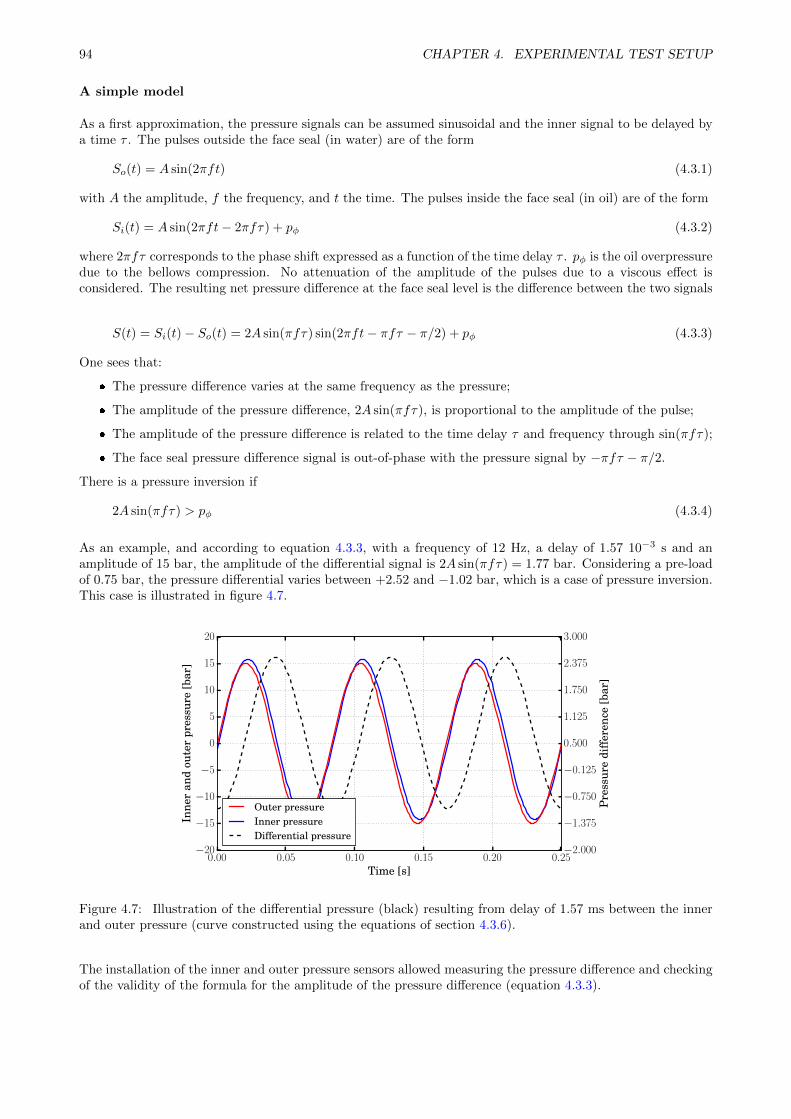
94 CHAPTER 4. EXPERIMENTAL TEST SETUP
A simple model
As a first approximation, the pressure signals can be assumed sinusoidal and the inner signal to be delayed bya time τ . The pulses outside the face seal (in water) are of the form
So(t) = A sin(2πft) (4.3.1)
with A the amplitude, f the frequency, and t the time. The pulses inside the face seal (in oil) are of the form
Si(t) = A sin(2πft− 2πfτ) + pφ (4.3.2)
where 2πfτ corresponds to the phase shift expressed as a function of the time delay τ . pφ is the oil overpressuredue to the bellows compression. No attenuation of the amplitude of the pulses due to a viscous effect isconsidered. The resulting net pressure difference at the face seal level is the difference between the two signals
S(t) = Si(t)− So(t) = 2A sin(πfτ) sin(2πft− πfτ − π/2) + pφ (4.3.3)
One sees that:
The pressure difference varies at the same frequency as the pressure;
The amplitude of the pressure difference, 2A sin(πfτ), is proportional to the amplitude of the pulse;
The amplitude of the pressure difference is related to the time delay τ and frequency through sin(πfτ);
The face seal pressure difference signal is out-of-phase with the pressure signal by −πfτ − π/2.
There is a pressure inversion if
2A sin(πfτ) > pφ (4.3.4)
As an example, and according to equation 4.3.3, with a frequency of 12 Hz, a delay of 1.57 10−3 s and anamplitude of 15 bar, the amplitude of the differential signal is 2A sin(πfτ) = 1.77 bar. Considering a pre-loadof 0.75 bar, the pressure differential varies between +2.52 and −1.02 bar, which is a case of pressure inversion.This case is illustrated in figure 4.7.
0.00 0.05 0.10 0.15 0.20 0.25Time [s]
−20
−15
−10
−5
0
5
10
15
20
Inne
ran
dou
ter
pres
sure
[bar
]
−2.000
−1.375
−0.750
−0.125
0.500
1.125
1.750
2.375
3.000
Pre
ssur
edi
ffer
ence
[bar
]
Outer pressureInner pressureDifferential pressure
Figure 4.7: Illustration of the differential pressure (black) resulting from delay of 1.57 ms between the innerand outer pressure (curve constructed using the equations of section 4.3.6).
The installation of the inner and outer pressure sensors allowed measuring the pressure difference and checkingof the validity of the formula for the amplitude of the pressure difference (equation 4.3.3).
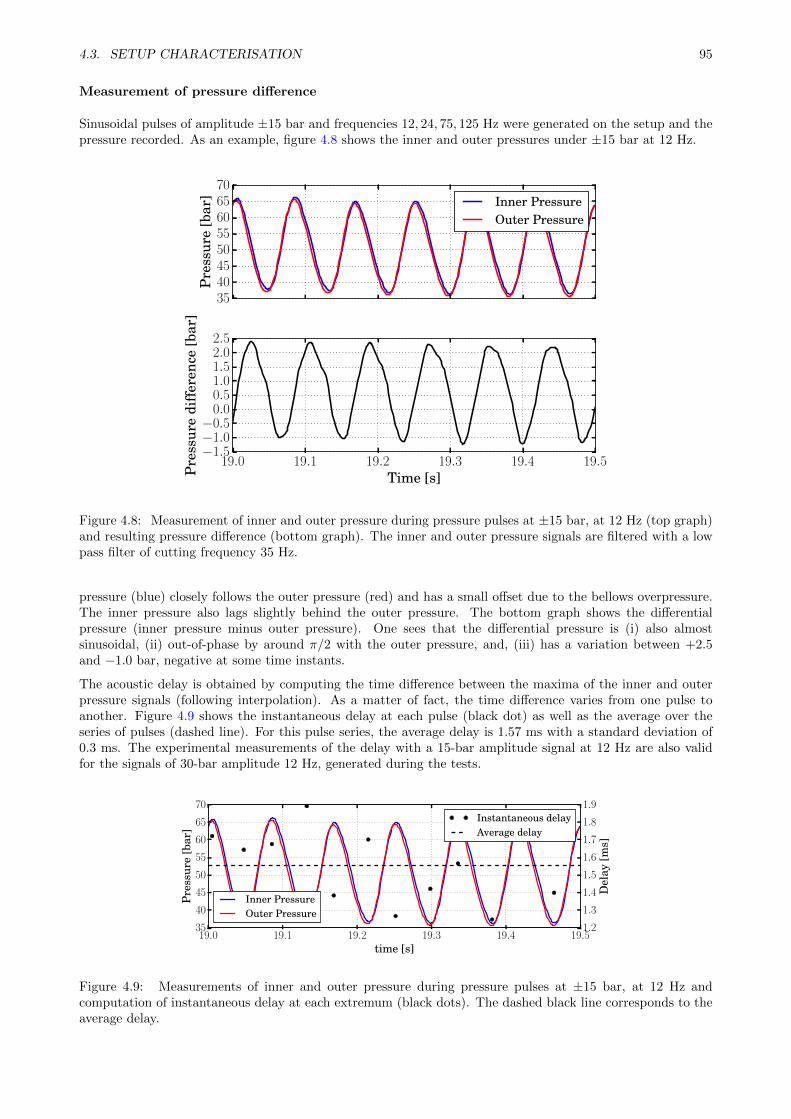
4.3. SETUP CHARACTERISATION 95
Measurement of pressure difference
Sinusoidal pulses of amplitude ±15 bar and frequencies 12, 24, 75, 125 Hz were generated on the setup and thepressure recorded. As an example, figure 4.8 shows the inner and outer pressures under ±15 bar at 12 Hz.
3540455055606570
Pre
ssur
e[b
ar] Inner Pressure
Outer Pressure
19.0 19.1 19.2 19.3 19.4 19.5Time [s]
−1.5−1.0−0.5
0.00.51.01.52.02.5
Pre
ssur
edi
ffer
ence
[bar
]
Figure 4.8: Measurement of inner and outer pressure during pressure pulses at ±15 bar, at 12 Hz (top graph)and resulting pressure difference (bottom graph). The inner and outer pressure signals are filtered with a lowpass filter of cutting frequency 35 Hz.
pressure (blue) closely follows the outer pressure (red) and has a small offset due to the bellows overpressure.The inner pressure also lags slightly behind the outer pressure. The bottom graph shows the differentialpressure (inner pressure minus outer pressure). One sees that the differential pressure is (i) also almostsinusoidal, (ii) out-of-phase by around π/2 with the outer pressure, and, (iii) has a variation between +2.5and −1.0 bar, negative at some time instants.
The acoustic delay is obtained by computing the time difference between the maxima of the inner and outerpressure signals (following interpolation). As a matter of fact, the time difference varies from one pulse toanother. Figure 4.9 shows the instantaneous delay at each pulse (black dot) as well as the average over theseries of pulses (dashed line). For this pulse series, the average delay is 1.57 ms with a standard deviation of0.3 ms. The experimental measurements of the delay with a 15-bar amplitude signal at 12 Hz are also validfor the signals of 30-bar amplitude 12 Hz, generated during the tests.
19.0 19.1 19.2 19.3 19.4 19.5time [s]
35
40
45
50
55
60
65
70
Pre
ssur
e[b
ar]
Inner PressureOuter Pressure
1.2
1.3
1.4
1.5
1.6
1.7
1.8
1.9
Del
ay[m
s]
Instantaneous delayAverage delay
Figure 4.9: Measurements of inner and outer pressure during pressure pulses at ±15 bar, at 12 Hz andcomputation of instantaneous delay at each extremum (black dots). The dashed black line corresponds to theaverage delay.
96 CHAPTER 4. EXPERIMENTAL TEST SETUP
The fact that (1) delays were measured and that (2) they lead to negative pressure differences validates thesetup as a tool to test face seals under pressure pulses, and negative pressure as stated in the goal setting.
Equation 4.3.3 predicts a pressure difference varying between 2.52 and −1.02 bar when the same signal pa-rameters and the average delay of 1.57 ms is considered. The amplitudes measured experimentally are veryclose to the values estimated with the formula, which validates the formula estimations of differential signalamplitudes from known delay, frequency, and amplitude.
Pressure difference at the face seal level for the pressure pulses used in the tests
The two previous subsections showed and validated an equation for the face seal pressure difference. Theyalso present measurements of the face seal holder delay of τ = 1.57 ms for pulses at 12 Hz. Based on theseresults, the amplitude of the pressure difference seen by the face seal when the face seal holder is subject tooperating pressure pulses of amplitude A = 30 bar at a frequency of f = 12 Hz is
2A sin(πfτ) = 2 · 30 · sin(π · 12 · 1.57 · 10−3) = 3.55 bar (4.3.5)
Further, considering an oil pre-load of pφ = 0.7 bar, the face seal pressure difference varies from +4.25 bar to−2.85 bar at 12 Hz. In an equivalent manner, when the setup generates pulses of ±30 bar at 12 Hz, the faceseal pressures are
pi = pback pressure + pφpo(t) = pback pressure + pdifference sin(2 · π · f · t) (4.3.6)
with pdifference = 3.55 · 105 Pa.
These values are also those used as boundary conditions for the numerical simulations presented in chapter 5.
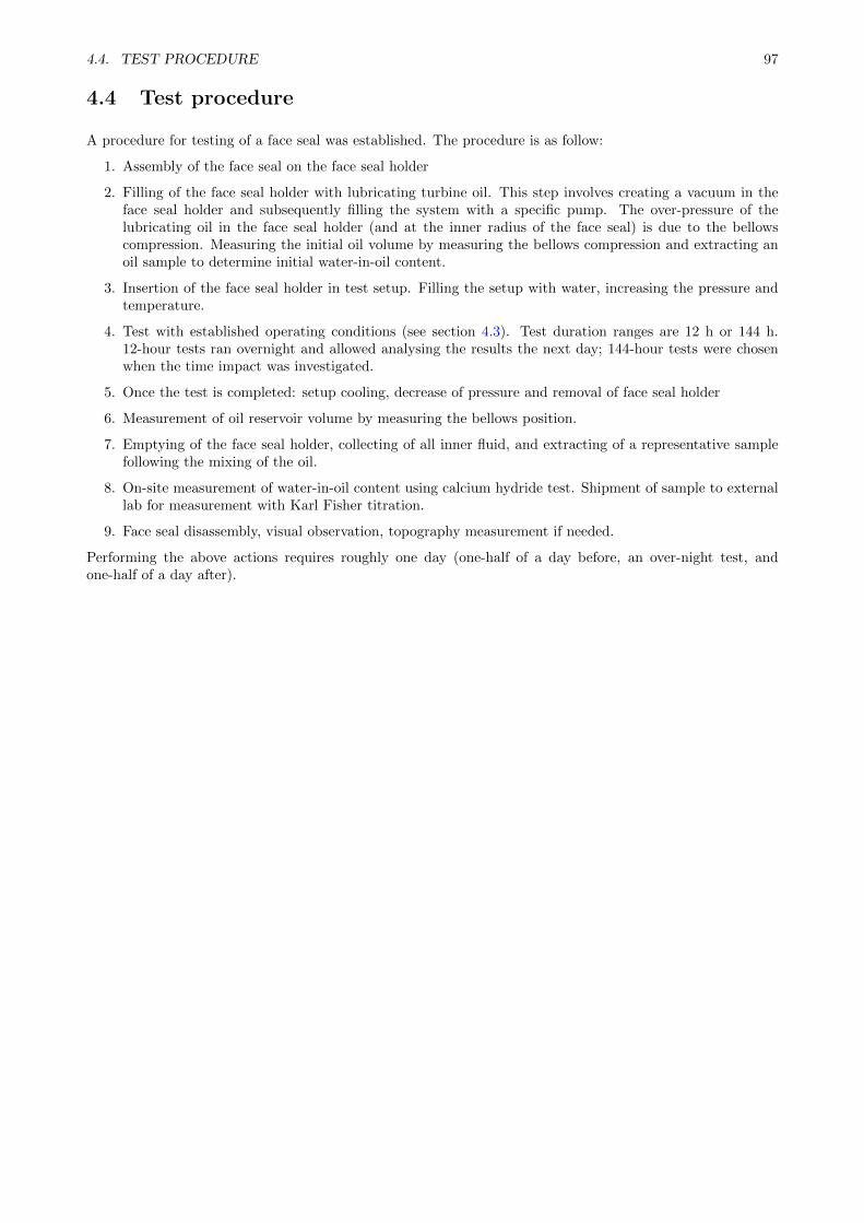
4.4. TEST PROCEDURE 97
4.4 Test procedure
A procedure for testing of a face seal was established. The procedure is as follow:
1. Assembly of the face seal on the face seal holder
2. Filling of the face seal holder with lubricating turbine oil. This step involves creating a vacuum in theface seal holder and subsequently filling the system with a specific pump. The over-pressure of thelubricating oil in the face seal holder (and at the inner radius of the face seal) is due to the bellowscompression. Measuring the initial oil volume by measuring the bellows compression and extracting anoil sample to determine initial water-in-oil content.
3. Insertion of the face seal holder in test setup. Filling the setup with water, increasing the pressure andtemperature.
4. Test with established operating conditions (see section 4.3). Test duration ranges are 12 h or 144 h.12-hour tests ran overnight and allowed analysing the results the next day; 144-hour tests were chosenwhen the time impact was investigated.
5. Once the test is completed: setup cooling, decrease of pressure and removal of face seal holder
6. Measurement of oil reservoir volume by measuring the bellows position.
7. Emptying of the face seal holder, collecting of all inner fluid, and extracting of a representative samplefollowing the mixing of the oil.
8. On-site measurement of water-in-oil content using calcium hydride test. Shipment of sample to externallab for measurement with Karl Fisher titration.
9. Face seal disassembly, visual observation, topography measurement if needed.
Performing the above actions requires roughly one day (one-half of a day before, an over-night test, andone-half of a day after).
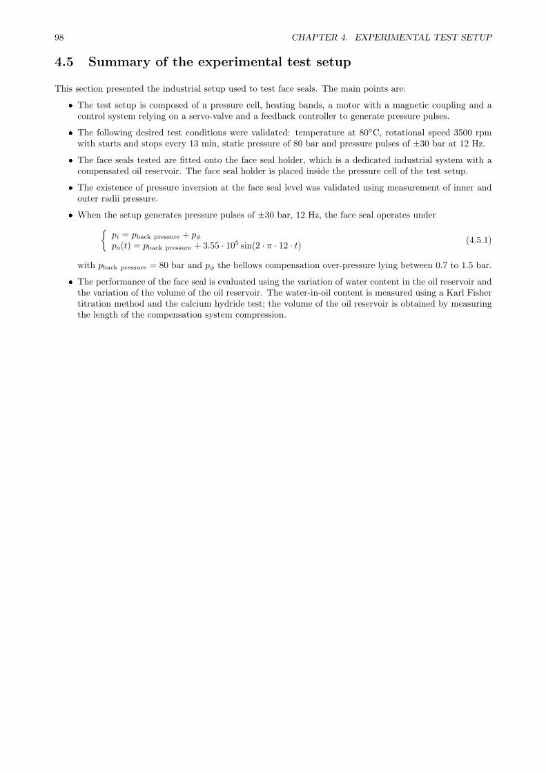
98 CHAPTER 4. EXPERIMENTAL TEST SETUP
4.5 Summary of the experimental test setup
This section presented the industrial setup used to test face seals. The main points are:
The test setup is composed of a pressure cell, heating bands, a motor with a magnetic coupling and acontrol system relying on a servo-valve and a feedback controller to generate pressure pulses.
The following desired test conditions were validated: temperature at 80C, rotational speed 3500 rpmwith starts and stops every 13 min, static pressure of 80 bar and pressure pulses of ±30 bar at 12 Hz.
The face seals tested are fitted onto the face seal holder, which is a dedicated industrial system with acompensated oil reservoir. The face seal holder is placed inside the pressure cell of the test setup.
The existence of pressure inversion at the face seal level was validated using measurement of inner andouter radii pressure.
When the setup generates pressure pulses of ±30 bar, 12 Hz, the face seal operates underpi = pback pressure + pφpo(t) = pback pressure + 3.55 · 105 sin(2 · π · 12 · t) (4.5.1)
with pback pressure = 80 bar and pφ the bellows compensation over-pressure lying between 0.7 to 1.5 bar.
The performance of the face seal is evaluated using the variation of water content in the oil reservoir andthe variation of the volume of the oil reservoir. The water-in-oil content is measured using a Karl Fishertitration method and the calcium hydride test; the volume of the oil reservoir is obtained by measuringthe length of the compensation system compression.
Chapter 5
Numerical and experimental results
The main objective of this section is to evaluate the amount of outer fluid ingression resulting from pressurepulses for a reference face seal, for a face seal with a misaligned rotor, and for a face seal with waviness. Thestudy is motivated by industrial interests. The results from a three series of tests on the experimental setupare analysed and simulated with the model developed.
Contents5.1 Face seal parameters and reference conditions . . . . . . . . . . . . . . . . . . . . 100
5.1.1 Geometry definition . . . . . . . . . . . . . . . . . . . . . . . . . . . . . . . . . . . . 100
5.1.2 Parameters of the reference face seal . . . . . . . . . . . . . . . . . . . . . . . . . . . 101
5.1.3 Face seal performance in reference conditions . . . . . . . . . . . . . . . . . . . . . . 101
5.2 Parametric study . . . . . . . . . . . . . . . . . . . . . . . . . . . . . . . . . . . . . 104
5.2.1 Impact of uncertainties of the inputs on the numerical predictions . . . . . . . . . . 104
5.2.2 Impact of the operating conditions on numerical predictions . . . . . . . . . . . . . . 108
5.2.3 Simulations of accelerations with transient thermal effects . . . . . . . . . . . . . . . 110
5.2.4 Modelling simplifications and numerical considerations . . . . . . . . . . . . . . . . 112
5.3 Effect of pressure pulses . . . . . . . . . . . . . . . . . . . . . . . . . . . . . . . . . 113
5.3.1 Experimental results with pressure pulses . . . . . . . . . . . . . . . . . . . . . . . . 113
5.3.2 Simulations with pressure pulses . . . . . . . . . . . . . . . . . . . . . . . . . . . . . 114
5.3.3 Conclusions from the study of pressure pulses . . . . . . . . . . . . . . . . . . . . . . 121
5.4 Effect of rotor misalignment . . . . . . . . . . . . . . . . . . . . . . . . . . . . . . . 122
5.4.1 Experimental results with rotor misalignment and pressure pulses . . . . . . . . . . 122
5.4.2 Simulations with a misaligned rotor . . . . . . . . . . . . . . . . . . . . . . . . . . . 123
5.4.3 Simulation with a rotor misalignment of 3.5 mrad and pressure pulses . . . . . . . . 127
5.4.4 Conclusions from the study of the face seal with rotor misalignment . . . . . . . . . 129
5.5 Effect of waviness . . . . . . . . . . . . . . . . . . . . . . . . . . . . . . . . . . . . . 130
5.5.1 Experimental results for the wavy face seal prototype under pressure pulses . . . . . 130
5.5.2 Simulation of the reference face seal with consideration of waviness . . . . . . . . . . 132
5.5.3 Simulation of the reference face seal with waviness and with pressure pulses . . . . . 141
5.5.4 Simulation of the wavy face seal prototype . . . . . . . . . . . . . . . . . . . . . . . 142
5.5.5 Conclusions from the study of the effect of face waviness . . . . . . . . . . . . . . . . 144
5.6 Summary of the main results of the studies and conclusion . . . . . . . . . . . . 145
5.6.1 Summary of the main results . . . . . . . . . . . . . . . . . . . . . . . . . . . . . . . 145
5.6.2 Conclusions from the experimental and numerical studies . . . . . . . . . . . . . . . 146
In the first place, the face seal is presented, followed by a parametric study performed with the numericalmodel. The study aims at evaluating the sensitivity of the predictions of the model to variations of the inputparameters to gain a better understanding of the face seal. In the second part, the experimental results arepresented and analysed along with the numerical simulations to provide insight into the behaviour of the faceseal under pressure pulses. The three studies are: face seal with pressure pulses, misaligned face seal withpressure pulses, and wavy face seal with pressure pulses. The test results are used to evaluate the capacity ofthe model to predict water entry. The face seal wear through analysis of the contact pressure is also discussed.
99
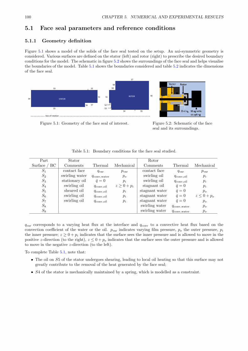
100 CHAPTER 5. NUMERICAL AND EXPERIMENTAL RESULTS
5.1 Face seal parameters and reference conditions
5.1.1 Geometry definition
Figure 5.1 shows a model of the solids of the face seal tested on the setup. An axi-symmetric geometry isconsidered. Various surfaces are defined on the stator (left) and rotor (right) to prescribe the desired boundaryconditions for the model. The schematic in figure 5.2 shows the surroundings of the face seal and helps visualisethe boundaries of the model. Table 5.1 shows the boundaries considered and table 5.2 indicates the dimensionsof the face seal.
STATORS1
S2S3
S4
S5
S6 S7
S1
S2
S3
S4 S5
S6
S7
S8
S9
ROTOR
Axis of rotation
Figure 5.1: Geometry of the face seal of interest.
Schlu
mb
erger Co
nfid
ential
Figure 5.2: Schematic of the faceseal and its surroundings.
Table 5.1: Boundary conditions for the face seal studied.
Part Stator RotorSurface / BC Comments Thermal Mechanical Comments Thermal Mechanical
S1 contact face qvar pvar contact face qvar pvar
S2 swirling water qconv,water po swirling oil qconv,oil piS3 stationary oil q = 0 pi swirling oil qconv,oil piS4 swirling oil qconv,oil z ≥ 0 + pi stagnant oil q = 0 piS5 sheared oil qconv,oil pi stagnant water q = 0 poS6 swirling oil qconv,oil pi stagnant water q = 0 z ≤ 0 + poS7 swirling oil qconv,oil pi stagnant water q = 0 poS8 swirling water qconv,water poS9 swirling water qconv,water po
qvar corresponds to a varying heat flux at the interface and qconv to a convective heat flux based on theconvection coefficient of the water or the oil. pvar indicates varying film pressure, po the outer pressure, pithe inner pressure; z ≥ 0 + pi indicates that the surface sees the inner pressure and is allowed to move in thepositive z-direction (to the right), z ≤ 0 + po indicates that the surface sees the outer pressure and is allowedto move in the negative z-direction (to the left).
To complete Table 5.1, note that:
The oil on S5 of the stator undergoes shearing, leading to local oil heating so that this surface may notgreatly contribute to the removal of the heat generated by the face seal;
S4 of the stator is mechanically maintained by a spring, which is modelled as a constraint.
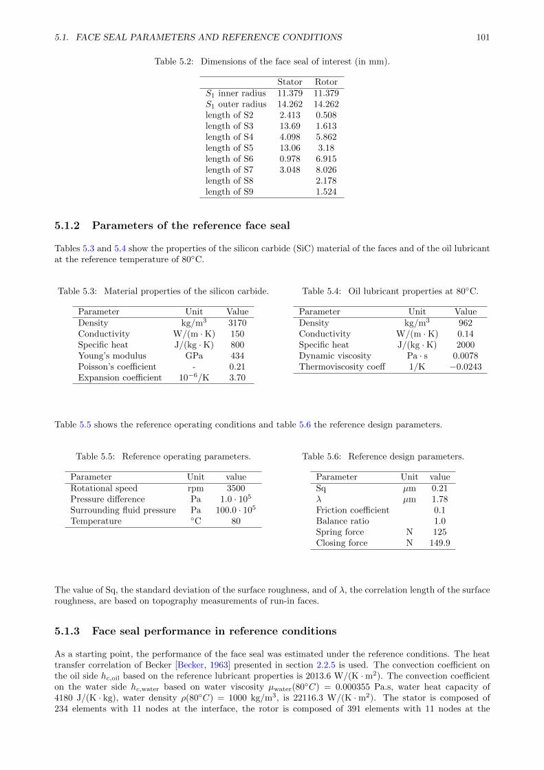
5.1. FACE SEAL PARAMETERS AND REFERENCE CONDITIONS 101
Table 5.2: Dimensions of the face seal of interest (in mm).
Stator RotorS1 inner radius 11.379 11.379S1 outer radius 14.262 14.262length of S2 2.413 0.508length of S3 13.69 1.613length of S4 4.098 5.862length of S5 13.06 3.18length of S6 0.978 6.915length of S7 3.048 8.026length of S8 2.178length of S9 1.524
5.1.2 Parameters of the reference face seal
Tables 5.3 and 5.4 show the properties of the silicon carbide (SiC) material of the faces and of the oil lubricantat the reference temperature of 80C.
Table 5.3: Material properties of the silicon carbide.
Parameter Unit ValueDensity kg/m3 3170Conductivity W/(m ·K) 150Specific heat J/(kg ·K) 800Young’s modulus GPa 434Poisson’s coefficient - 0.21Expansion coefficient 10−6/K 3.70
Table 5.4: Oil lubricant properties at 80C.
Parameter Unit ValueDensity kg/m3 962Conductivity W/(m ·K) 0.14Specific heat J/(kg ·K) 2000Dynamic viscosity Pa · s 0.0078Thermoviscosity coeff 1/K −0.0243
Table 5.5 shows the reference operating conditions and table 5.6 the reference design parameters.
Table 5.5: Reference operating parameters.
Parameter Unit valueRotational speed rpm 3500Pressure difference Pa 1.0 · 105
Surrounding fluid pressure Pa 100.0 · 105
Temperature C 80
Table 5.6: Reference design parameters.
Parameter Unit valueSq µm 0.21λ µm 1.78Friction coefficient 0.1Balance ratio 1.0Spring force N 125Closing force N 149.9
The value of Sq, the standard deviation of the surface roughness, and of λ, the correlation length of the surfaceroughness, are based on topography measurements of run-in faces.
5.1.3 Face seal performance in reference conditions
As a starting point, the performance of the face seal was estimated under the reference conditions. The heattransfer correlation of Becker [Becker, 1963] presented in section 2.2.5 is used. The convection coefficient onthe oil side hc,oil based on the reference lubricant properties is 2013.6 W/(K ·m2). The convection coefficienton the water side hc,water based on water viscosity µwater(80C) = 0.000355 Pa.s, water heat capacity of4180 J/(K · kg), water density ρ(80C) = 1000 kg/m3, is 22116.3 W/(K ·m2). The stator is composed of234 elements with 11 nodes at the interface, the rotor is composed of 391 elements with 11 nodes at the
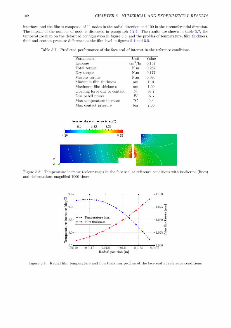
102 CHAPTER 5. NUMERICAL AND EXPERIMENTAL RESULTS
interface, and the film is composed of 11 nodes in the radial direction and 100 in the circumferential direction.The impact of the number of node is discussed in paragraph 5.2.4. The results are shown in table 5.7, thetemperature map on the deformed configuration in figure 5.3, and the profiles of temperature, film thickness,fluid and contact pressure difference at the film level in figures 5.4 and 5.5.
Table 5.7: Predicted performance of the face seal of interest in the reference conditions.
Parameters Unit ValueLeakage cm3/hr 0.137Total torque N.m 0.267Dry torque N.m 0.177Viscous torque N.m 0.090Minimum film thickness µm 1.01Maximum film thickness µm 1.09Opening force due to contact % 93.7Dissipated power W 97.7Max temperature increase C 9.3Max contact pressure bar 7.60
Figure 5.3: Temperature increase (colour map) in the face seal at reference conditions with isotherms (lines)and deformations magnified 1000 times.
0.0110 0.0117 0.0124 0.0131 0.0138 0.0145Radial position [m]
7.5
8.0
8.5
9.0
9.5
Tem
pera
ture
incr
ease
[deg
C]
1.000
1.025
1.050
1.075
1.100
Film
thic
knes
s[µ
m]
Temperature incr.Film thickness
Figure 5.4: Radial film temperature and film thickness profiles of the face seal at reference conditions.
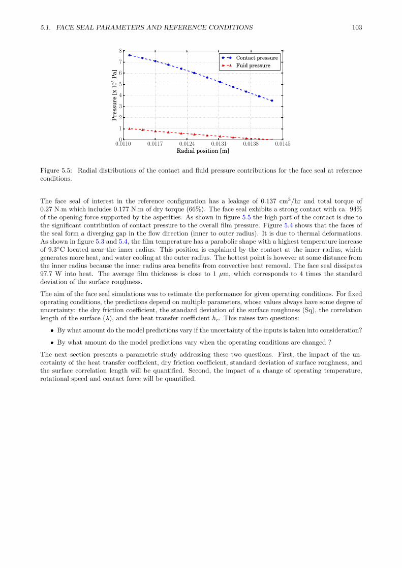
5.1. FACE SEAL PARAMETERS AND REFERENCE CONDITIONS 103
0.0110 0.0117 0.0124 0.0131 0.0138 0.0145Radial position [m]
0
1
2
3
4
5
6
7
8
Pre
ssur
e[x
105
Pa]
Contact pressureFuid pressure
Figure 5.5: Radial distributions of the contact and fluid pressure contributions for the face seal at referenceconditions.
The face seal of interest in the reference configuration has a leakage of 0.137 cm3/hr and total torque of0.27 N.m which includes 0.177 N.m of dry torque (66%). The face seal exhibits a strong contact with ca. 94%of the opening force supported by the asperities. As shown in figure 5.5 the high part of the contact is due tothe significant contribution of contact pressure to the overall film pressure. Figure 5.4 shows that the faces ofthe seal form a diverging gap in the flow direction (inner to outer radius). It is due to thermal deformations.As shown in figure 5.3 and 5.4, the film temperature has a parabolic shape with a highest temperature increaseof 9.3C located near the inner radius. This position is explained by the contact at the inner radius, whichgenerates more heat, and water cooling at the outer radius. The hottest point is however at some distance fromthe inner radius because the inner radius area benefits from convective heat removal. The face seal dissipates97.7 W into heat. The average film thickness is close to 1 µm, which corresponds to 4 times the standarddeviation of the surface roughness.
The aim of the face seal simulations was to estimate the performance for given operating conditions. For fixedoperating conditions, the predictions depend on multiple parameters, whose values always have some degree ofuncertainty: the dry friction coefficient, the standard deviation of the surface roughness (Sq), the correlationlength of the surface (λ), and the heat transfer coefficient hc. This raises two questions:
By what amount do the model predictions vary if the uncertainty of the inputs is taken into consideration?
By what amount do the model predictions vary when the operating conditions are changed ?
The next section presents a parametric study addressing these two questions. First, the impact of the un-certainty of the heat transfer coefficient, dry friction coefficient, standard deviation of surface roughness, andthe surface correlation length will be quantified. Second, the impact of a change of operating temperature,rotational speed and contact force will be quantified.
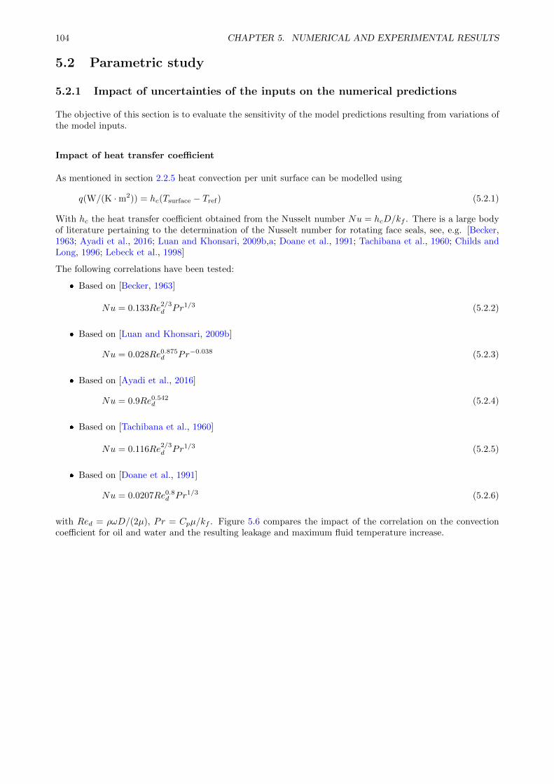
104 CHAPTER 5. NUMERICAL AND EXPERIMENTAL RESULTS
5.2 Parametric study
5.2.1 Impact of uncertainties of the inputs on the numerical predictions
The objective of this section is to evaluate the sensitivity of the model predictions resulting from variations ofthe model inputs.
Impact of heat transfer coefficient
As mentioned in section 2.2.5 heat convection per unit surface can be modelled using
q(W/(K ·m2)) = hc(Tsurface − Tref) (5.2.1)
With hc the heat transfer coefficient obtained from the Nusselt number Nu = hcD/kf . There is a large bodyof literature pertaining to the determination of the Nusselt number for rotating face seals, see, e.g. [Becker,1963; Ayadi et al., 2016; Luan and Khonsari, 2009b,a; Doane et al., 1991; Tachibana et al., 1960; Childs andLong, 1996; Lebeck et al., 1998]
The following correlations have been tested:
Based on [Becker, 1963]
Nu = 0.133Re2/3d Pr1/3 (5.2.2)
Based on [Luan and Khonsari, 2009b]
Nu = 0.028Re0.875d Pr−0.038 (5.2.3)
Based on [Ayadi et al., 2016]
Nu = 0.9Re0.542d (5.2.4)
Based on [Tachibana et al., 1960]
Nu = 0.116Re2/3d Pr1/3 (5.2.5)
Based on [Doane et al., 1991]
Nu = 0.0207Re0.8d Pr1/3 (5.2.6)
with Red = ρωD/(2µ), Pr = Cpµ/kf . Figure 5.6 compares the impact of the correlation on the convectioncoefficient for oil and water and the resulting leakage and maximum fluid temperature increase.
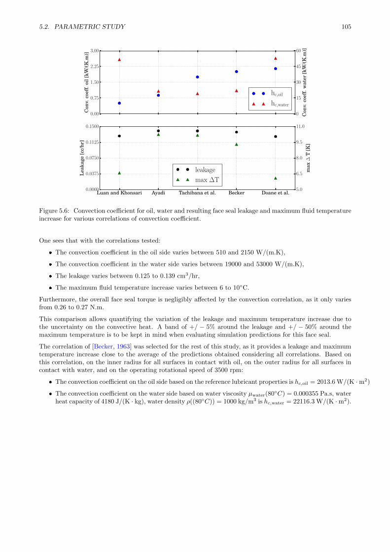
5.2. PARAMETRIC STUDY 105
0.00
0.75
1.50
2.25
3.00
Con
v.co
eff.
oil[
kW/(K
.m)]
hc,oil
hc,water
Luan and Khonsari Ayadi Tachibana et al. Becker Doane et al.0.0000
0.0375
0.0750
0.1125
0.1500
Lea
kage
[cc/
hr]
leakage
max ∆T
0
15
30
45
60
Con
v.co
eff.
wat
er[k
W/(K
.m)]
5.0
6.5
8.0
9.5
11.0
max
∆T
[K]
Figure 5.6: Convection coefficient for oil, water and resulting face seal leakage and maximum fluid temperatureincrease for various correlations of convection coefficient.
One sees that with the correlations tested:
The convection coefficient in the oil side varies between 510 and 2150 W/(m.K),
The convection coefficient in the water side varies between 19000 and 53000 W/(m.K),
The leakage varies between 0.125 to 0.139 cm3/hr,
The maximum fluid temperature increase varies between 6 to 10C.
Furthermore, the overall face seal torque is negligibly affected by the convection correlation, as it only variesfrom 0.26 to 0.27 N.m.
This comparison allows quantifying the variation of the leakage and maximum temperature increase due tothe uncertainty on the convective heat. A band of +/ − 5% around the leakage and +/ − 50% around themaximum temperature is to be kept in mind when evaluating simulation predictions for this face seal.
The correlation of [Becker, 1963] was selected for the rest of this study, as it provides a leakage and maximumtemperature increase close to the average of the predictions obtained considering all correlations. Based onthis correlation, on the inner radius for all surfaces in contact with oil, on the outer radius for all surfaces incontact with water, and on the operating rotational speed of 3500 rpm:
The convection coefficient on the oil side based on the reference lubricant properties is hc,oil = 2013.6 W/(K ·m2)
The convection coefficient on the water side based on water viscosity µwater(80C) = 0.000355 Pa.s, waterheat capacity of 4180 J/(K · kg), water density ρ((80C)) = 1000 kg/m3 is hc,water = 22116.3 W/(K ·m2).
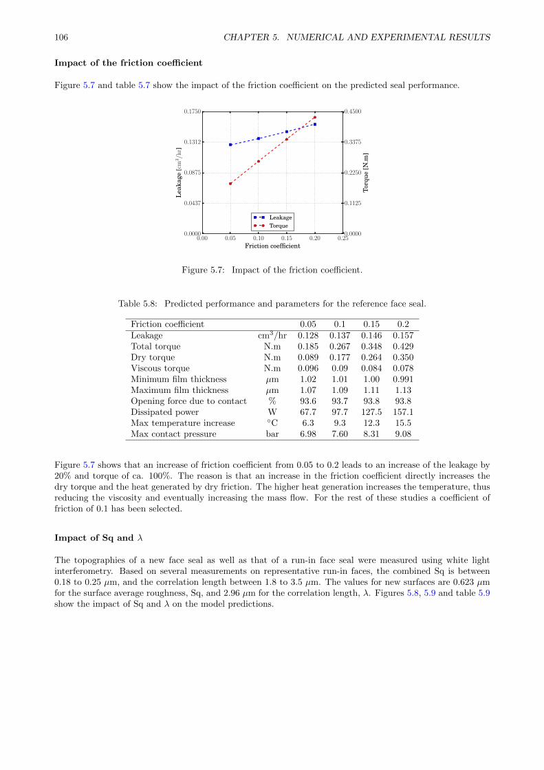
106 CHAPTER 5. NUMERICAL AND EXPERIMENTAL RESULTS
Impact of the friction coefficient
Figure 5.7 and table 5.7 show the impact of the friction coefficient on the predicted seal performance.
0.00 0.05 0.10 0.15 0.20 0.25Friction coefficient
0.0000
0.0437
0.0875
0.1312
0.1750
Lea
kage
[cm
3/h
r]
LeakageTorque
0.0000
0.1125
0.2250
0.3375
0.4500
Torq
ue[N
.m]
Figure 5.7: Impact of the friction coefficient.
Table 5.8: Predicted performance and parameters for the reference face seal.
Friction coefficient 0.05 0.1 0.15 0.2Leakage cm3/hr 0.128 0.137 0.146 0.157Total torque N.m 0.185 0.267 0.348 0.429Dry torque N.m 0.089 0.177 0.264 0.350Viscous torque N.m 0.096 0.09 0.084 0.078Minimum film thickness µm 1.02 1.01 1.00 0.991Maximum film thickness µm 1.07 1.09 1.11 1.13Opening force due to contact % 93.6 93.7 93.8 93.8Dissipated power W 67.7 97.7 127.5 157.1Max temperature increase C 6.3 9.3 12.3 15.5Max contact pressure bar 6.98 7.60 8.31 9.08
Figure 5.7 shows that an increase of friction coefficient from 0.05 to 0.2 leads to an increase of the leakage by20% and torque of ca. 100%. The reason is that an increase in the friction coefficient directly increases thedry torque and the heat generated by dry friction. The higher heat generation increases the temperature, thusreducing the viscosity and eventually increasing the mass flow. For the rest of these studies a coefficient offriction of 0.1 has been selected.
Impact of Sq and λ
The topographies of a new face seal as well as that of a run-in face seal were measured using white lightinterferometry. Based on several measurements on representative run-in faces, the combined Sq is between0.18 to 0.25 µm, and the correlation length between 1.8 to 3.5 µm. The values for new surfaces are 0.623 µmfor the surface average roughness, Sq, and 2.96 µm for the correlation length, λ. Figures 5.8, 5.9 and table 5.9show the impact of Sq and λ on the model predictions.
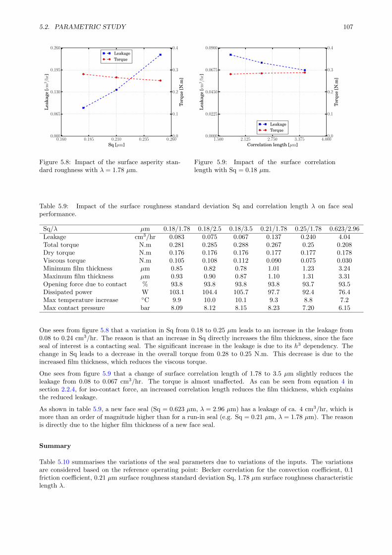
5.2. PARAMETRIC STUDY 107
0.160 0.185 0.210 0.235 0.260Sq [µm]
0.000
0.065
0.130
0.195
0.260L
eaka
ge[c
m3/h
r]
LeakageTorque
0.0
0.1
0.2
0.3
0.4
Torq
ue[N
.m]
Figure 5.8: Impact of the surface asperity stan-dard roughness with λ = 1.78 µm.
1.500 2.125 2.750 3.375 4.000Correlation length [µm]
0.0000
0.0225
0.0450
0.0675
0.0900
Lea
kage
[cm
3/h
r]
LeakageTorque
0.0
0.1
0.2
0.3
0.4
Torq
ue[N
.m]
Figure 5.9: Impact of the surface correlationlength with Sq = 0.18 µm.
Table 5.9: Impact of the surface roughness standard deviation Sq and correlation length λ on face sealperformance.
Sq/λ µm 0.18/1.78 0.18/2.5 0.18/3.5 0.21/1.78 0.25/1.78 0.623/2.96Leakage cm3/hr 0.083 0.075 0.067 0.137 0.240 4.04Total torque N.m 0.281 0.285 0.288 0.267 0.25 0.208Dry torque N.m 0.176 0.176 0.176 0.177 0.177 0.178Viscous torque N.m 0.105 0.108 0.112 0.090 0.075 0.030Minimum film thickness µm 0.85 0.82 0.78 1.01 1.23 3.24Maximum film thickness µm 0.93 0.90 0.87 1.10 1.31 3.31Opening force due to contact % 93.8 93.8 93.8 93.8 93.7 93.5Dissipated power W 103.1 104.4 105.7 97.7 92.4 76.4Max temperature increase C 9.9 10.0 10.1 9.3 8.8 7.2Max contact pressure bar 8.09 8.12 8.15 8.23 7.20 6.15
One sees from figure 5.8 that a variation in Sq from 0.18 to 0.25 µm leads to an increase in the leakage from0.08 to 0.24 cm3/hr. The reason is that an increase in Sq directly increases the film thickness, since the faceseal of interest is a contacting seal. The significant increase in the leakage is due to its h3 dependency. Thechange in Sq leads to a decrease in the overall torque from 0.28 to 0.25 N.m. This decrease is due to theincreased film thickness, which reduces the viscous torque.
One sees from figure 5.9 that a change of surface correlation length of 1.78 to 3.5 µm slightly reduces theleakage from 0.08 to 0.067 cm3/hr. The torque is almost unaffected. As can be seen from equation 4 insection 2.2.4, for iso-contact force, an increased correlation length reduces the film thickness, which explainsthe reduced leakage.
As shown in table 5.9, a new face seal (Sq = 0.623 µm, λ = 2.96 µm) has a leakage of ca. 4 cm3/hr, which ismore than an order of magnitude higher than for a run-in seal (e.g. Sq = 0.21 µm, λ = 1.78 µm). The reasonis directly due to the higher film thickness of a new face seal.
Summary
Table 5.10 summarises the variations of the seal parameters due to variations of the inputs. The variationsare considered based on the reference operating point: Becker correlation for the convection coefficient, 0.1friction coefficient, 0.21 µm surface roughness standard deviation Sq, 1.78 µm surface roughness characteristiclength λ.
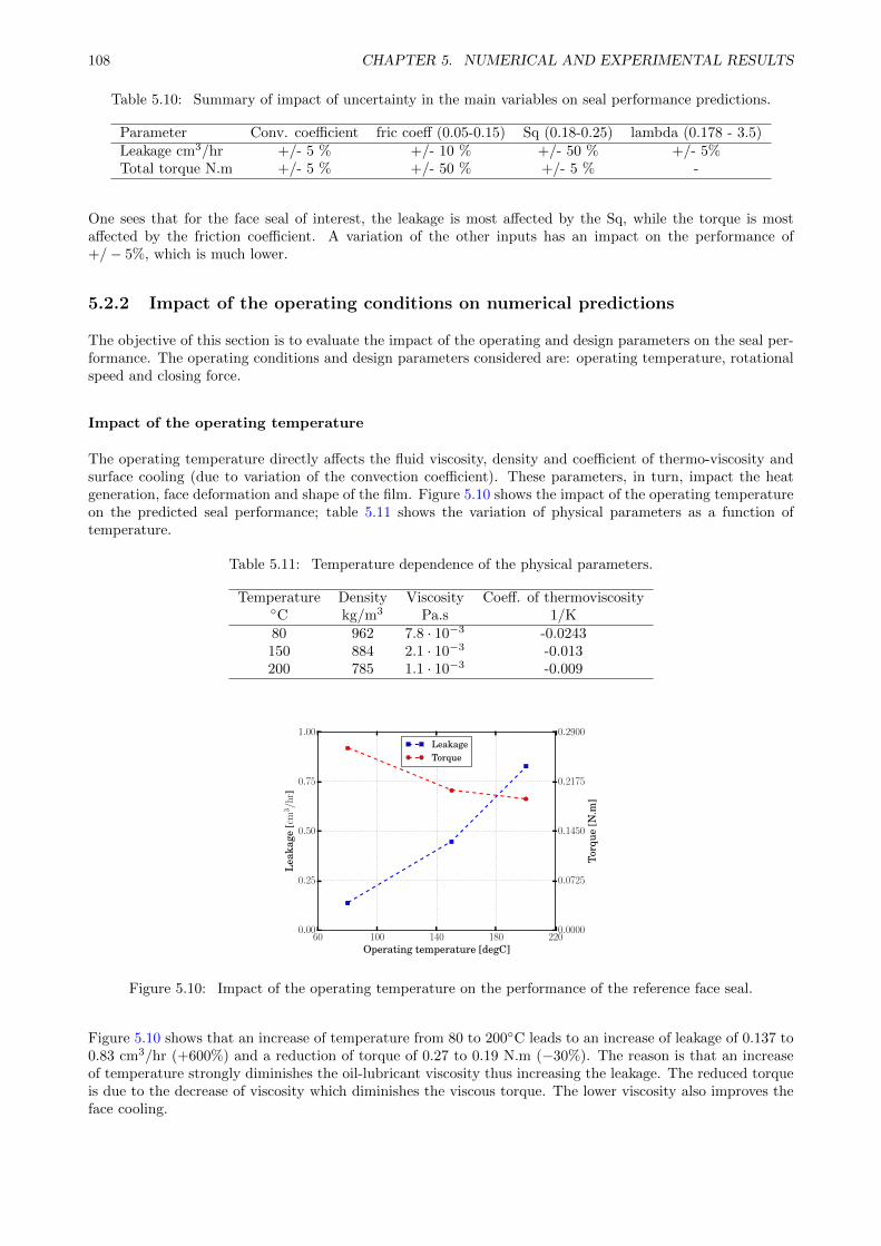
108 CHAPTER 5. NUMERICAL AND EXPERIMENTAL RESULTS
Table 5.10: Summary of impact of uncertainty in the main variables on seal performance predictions.
Parameter Conv. coefficient fric coeff (0.05-0.15) Sq (0.18-0.25) lambda (0.178 - 3.5)Leakage cm3/hr +/- 5 % +/- 10 % +/- 50 % +/- 5%Total torque N.m +/- 5 % +/- 50 % +/- 5 % -
One sees that for the face seal of interest, the leakage is most affected by the Sq, while the torque is mostaffected by the friction coefficient. A variation of the other inputs has an impact on the performance of+/− 5%, which is much lower.
5.2.2 Impact of the operating conditions on numerical predictions
The objective of this section is to evaluate the impact of the operating and design parameters on the seal per-formance. The operating conditions and design parameters considered are: operating temperature, rotationalspeed and closing force.
Impact of the operating temperature
The operating temperature directly affects the fluid viscosity, density and coefficient of thermo-viscosity andsurface cooling (due to variation of the convection coefficient). These parameters, in turn, impact the heatgeneration, face deformation and shape of the film. Figure 5.10 shows the impact of the operating temperatureon the predicted seal performance; table 5.11 shows the variation of physical parameters as a function oftemperature.
Table 5.11: Temperature dependence of the physical parameters.
Temperature Density Viscosity Coeff. of thermoviscosityC kg/m3 Pa.s 1/K80 962 7.8 · 10−3 -0.0243150 884 2.1 · 10−3 -0.013200 785 1.1 · 10−3 -0.009
60 100 140 180 220Operating temperature [degC]
0.00
0.25
0.50
0.75
1.00
Lea
kage
[cm
3/h
r]
LeakageTorque
0.0000
0.0725
0.1450
0.2175
0.2900
Torq
ue[N
.m]
Figure 5.10: Impact of the operating temperature on the performance of the reference face seal.
Figure 5.10 shows that an increase of temperature from 80 to 200C leads to an increase of leakage of 0.137 to0.83 cm3/hr (+600%) and a reduction of torque of 0.27 to 0.19 N.m (−30%). The reason is that an increaseof temperature strongly diminishes the oil-lubricant viscosity thus increasing the leakage. The reduced torqueis due to the decrease of viscosity which diminishes the viscous torque. The lower viscosity also improves theface cooling.
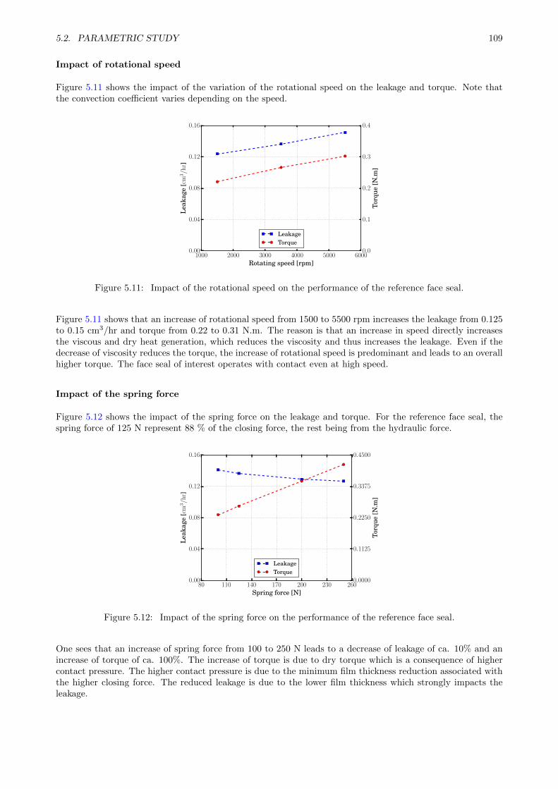
5.2. PARAMETRIC STUDY 109
Impact of rotational speed
Figure 5.11 shows the impact of the variation of the rotational speed on the leakage and torque. Note thatthe convection coefficient varies depending on the speed.
1000 2000 3000 4000 5000 6000Rotating speed [rpm]
0.00
0.04
0.08
0.12
0.16
Lea
kage
[cm
3/h
r]
LeakageTorque
0.0
0.1
0.2
0.3
0.4
Torq
ue[N
.m]
Figure 5.11: Impact of the rotational speed on the performance of the reference face seal.
Figure 5.11 shows that an increase of rotational speed from 1500 to 5500 rpm increases the leakage from 0.125to 0.15 cm3/hr and torque from 0.22 to 0.31 N.m. The reason is that an increase in speed directly increasesthe viscous and dry heat generation, which reduces the viscosity and thus increases the leakage. Even if thedecrease of viscosity reduces the torque, the increase of rotational speed is predominant and leads to an overallhigher torque. The face seal of interest operates with contact even at high speed.
Impact of the spring force
Figure 5.12 shows the impact of the spring force on the leakage and torque. For the reference face seal, thespring force of 125 N represent 88 % of the closing force, the rest being from the hydraulic force.
80 110 140 170 200 230 260Spring force [N]
0.00
0.04
0.08
0.12
0.16
Lea
kage
[cm
3/h
r]
LeakageTorque
0.0000
0.1125
0.2250
0.3375
0.4500
Torq
ue[N
.m]
Figure 5.12: Impact of the spring force on the performance of the reference face seal.
One sees that an increase of spring force from 100 to 250 N leads to a decrease of leakage of ca. 10% and anincrease of torque of ca. 100%. The increase of torque is due to dry torque which is a consequence of highercontact pressure. The higher contact pressure is due to the minimum film thickness reduction associated withthe higher closing force. The reduced leakage is due to the lower film thickness which strongly impacts theleakage.
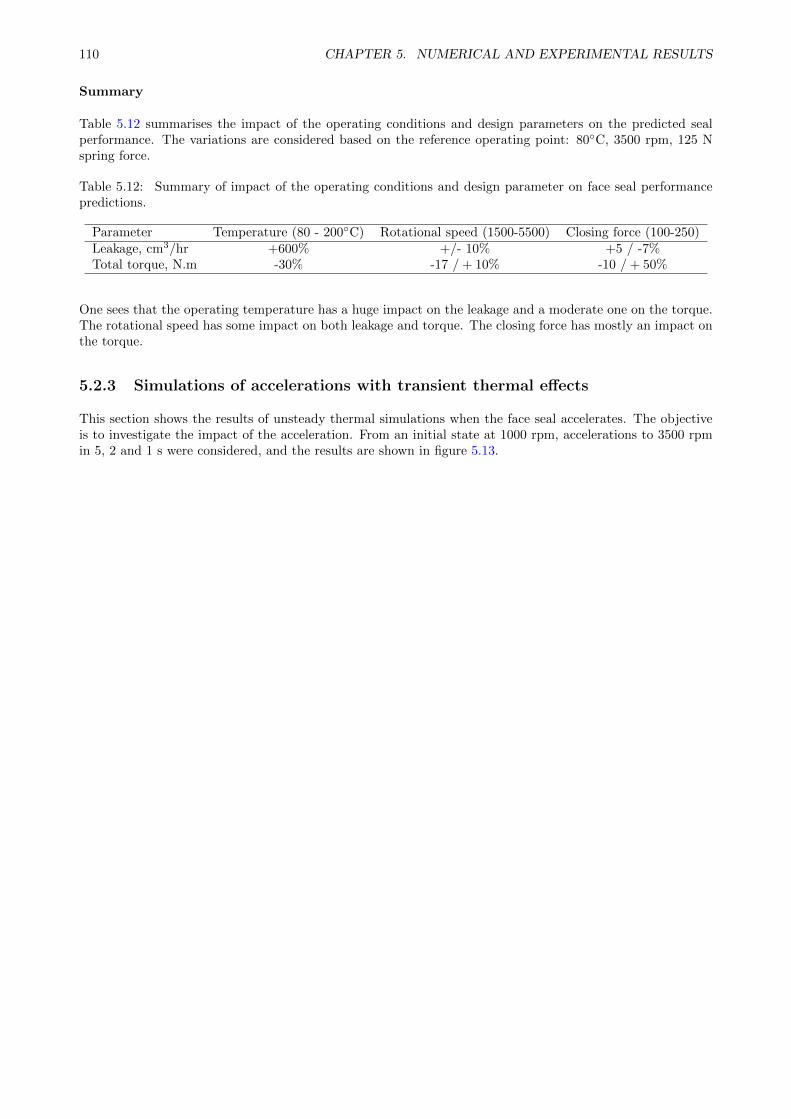
110 CHAPTER 5. NUMERICAL AND EXPERIMENTAL RESULTS
Summary
Table 5.12 summarises the impact of the operating conditions and design parameters on the predicted sealperformance. The variations are considered based on the reference operating point: 80C, 3500 rpm, 125 Nspring force.
Table 5.12: Summary of impact of the operating conditions and design parameter on face seal performancepredictions.
Parameter Temperature (80 - 200C) Rotational speed (1500-5500) Closing force (100-250)Leakage, cm3/hr +600% +/- 10% +5 / -7%Total torque, N.m -30% -17 /+ 10% -10 /+ 50%
One sees that the operating temperature has a huge impact on the leakage and a moderate one on the torque.The rotational speed has some impact on both leakage and torque. The closing force has mostly an impact onthe torque.
5.2.3 Simulations of accelerations with transient thermal effects
This section shows the results of unsteady thermal simulations when the face seal accelerates. The objectiveis to investigate the impact of the acceleration. From an initial state at 1000 rpm, accelerations to 3500 rpmin 5, 2 and 1 s were considered, and the results are shown in figure 5.13.
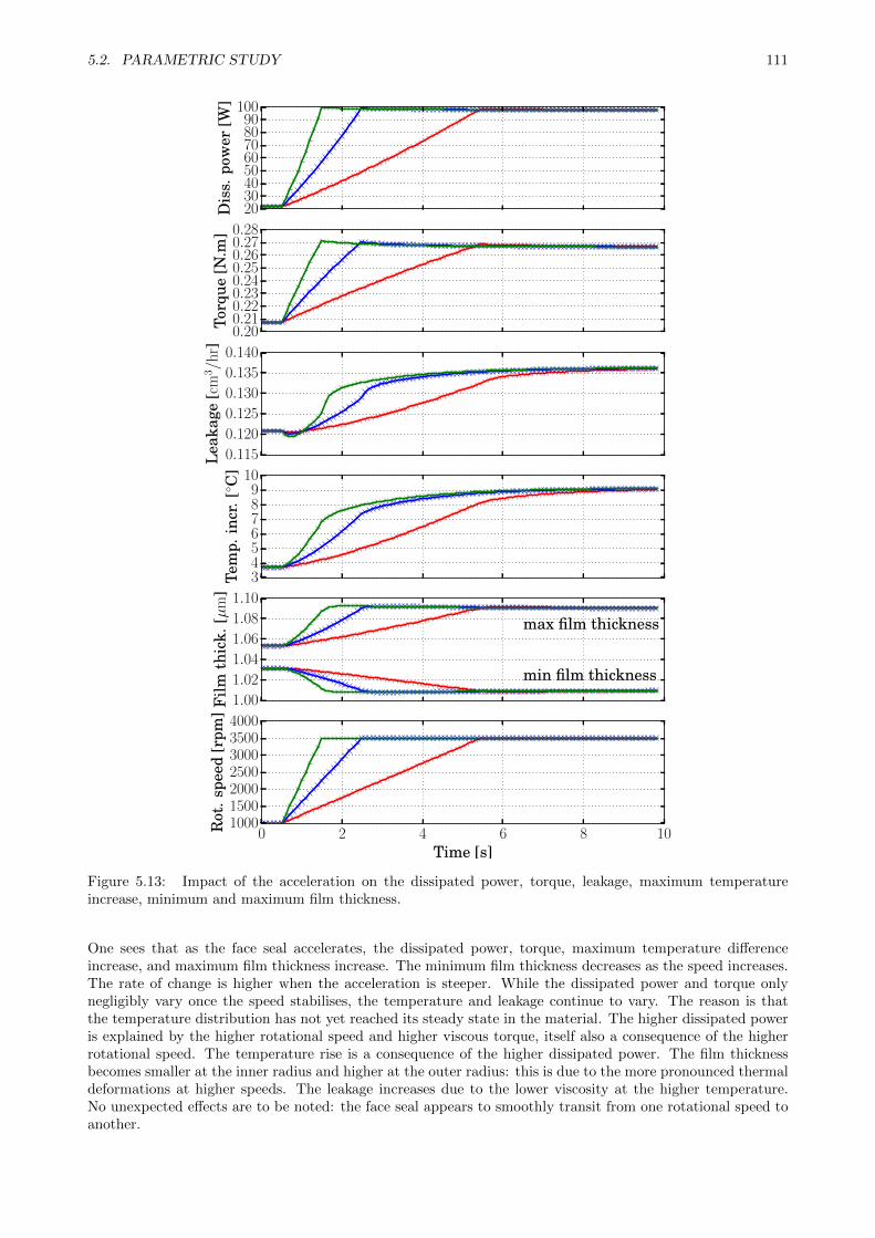
5.2. PARAMETRIC STUDY 111
2030405060708090
100
Dis
s.po
wer
[W]
0.200.210.220.230.240.250.260.270.28
Torq
ue[N
.m]
0.115
0.120
0.125
0.130
0.135
0.140
Lea
kage
[cm
3/h
r]
3456789
10
Tem
p.in
cr.[ C
]
1.00
1.02
1.04
1.06
1.08
1.10
Film
thic
k.[µ
m]
max film thickness
min film thickness
0 2 4 6 8 10Time [s]
1000150020002500300035004000
Rot
.spe
ed[r
pm]
Figure 5.13: Impact of the acceleration on the dissipated power, torque, leakage, maximum temperatureincrease, minimum and maximum film thickness.
One sees that as the face seal accelerates, the dissipated power, torque, maximum temperature differenceincrease, and maximum film thickness increase. The minimum film thickness decreases as the speed increases.The rate of change is higher when the acceleration is steeper. While the dissipated power and torque onlynegligibly vary once the speed stabilises, the temperature and leakage continue to vary. The reason is thatthe temperature distribution has not yet reached its steady state in the material. The higher dissipated poweris explained by the higher rotational speed and higher viscous torque, itself also a consequence of the higherrotational speed. The temperature rise is a consequence of the higher dissipated power. The film thicknessbecomes smaller at the inner radius and higher at the outer radius: this is due to the more pronounced thermaldeformations at higher speeds. The leakage increases due to the lower viscosity at the higher temperature.No unexpected effects are to be noted: the face seal appears to smoothly transit from one rotational speed toanother.
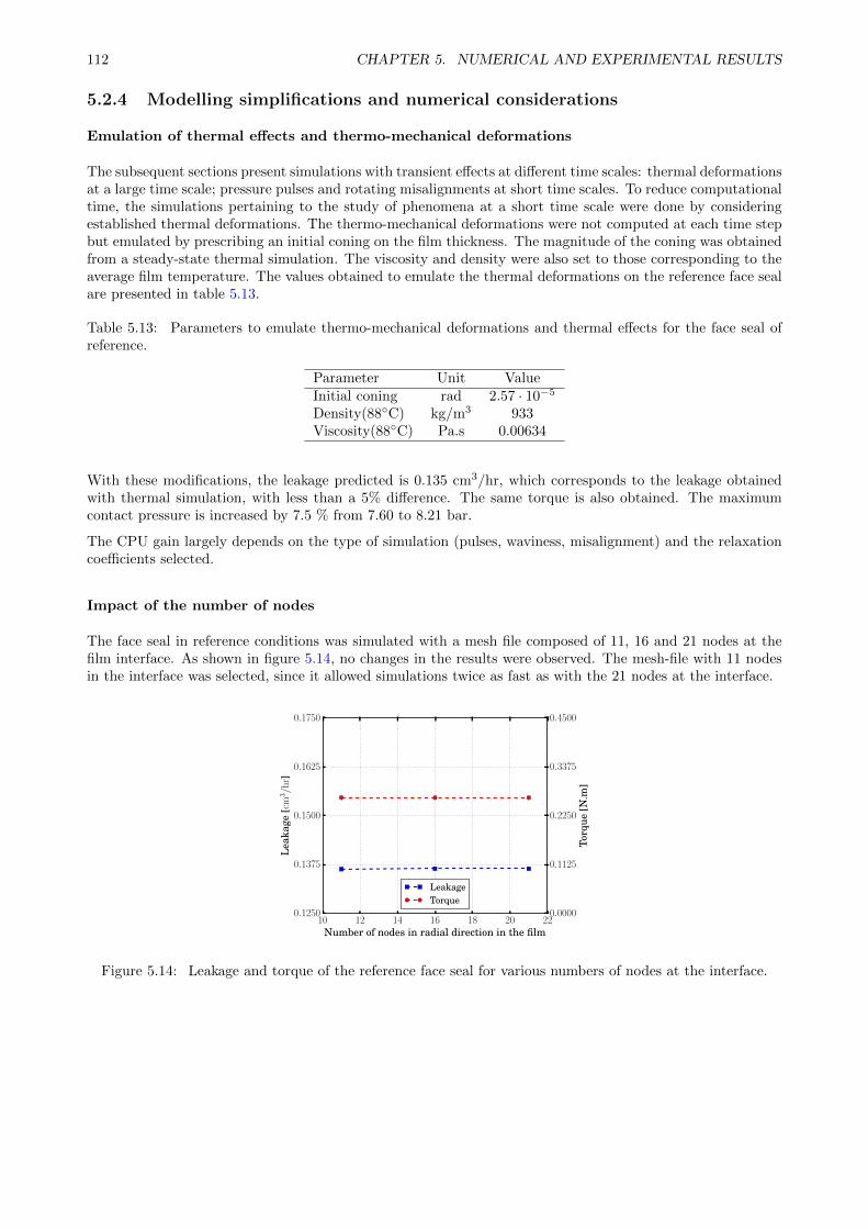
112 CHAPTER 5. NUMERICAL AND EXPERIMENTAL RESULTS
5.2.4 Modelling simplifications and numerical considerations
Emulation of thermal effects and thermo-mechanical deformations
The subsequent sections present simulations with transient effects at different time scales: thermal deformationsat a large time scale; pressure pulses and rotating misalignments at short time scales. To reduce computationaltime, the simulations pertaining to the study of phenomena at a short time scale were done by consideringestablished thermal deformations. The thermo-mechanical deformations were not computed at each time stepbut emulated by prescribing an initial coning on the film thickness. The magnitude of the coning was obtainedfrom a steady-state thermal simulation. The viscosity and density were also set to those corresponding to theaverage film temperature. The values obtained to emulate the thermal deformations on the reference face sealare presented in table 5.13.
Table 5.13: Parameters to emulate thermo-mechanical deformations and thermal effects for the face seal ofreference.
Parameter Unit ValueInitial coning rad 2.57 · 10−5
Density(88C) kg/m3 933Viscosity(88C) Pa.s 0.00634
With these modifications, the leakage predicted is 0.135 cm3/hr, which corresponds to the leakage obtainedwith thermal simulation, with less than a 5% difference. The same torque is also obtained. The maximumcontact pressure is increased by 7.5 % from 7.60 to 8.21 bar.
The CPU gain largely depends on the type of simulation (pulses, waviness, misalignment) and the relaxationcoefficients selected.
Impact of the number of nodes
The face seal in reference conditions was simulated with a mesh file composed of 11, 16 and 21 nodes at thefilm interface. As shown in figure 5.14, no changes in the results were observed. The mesh-file with 11 nodesin the interface was selected, since it allowed simulations twice as fast as with the 21 nodes at the interface.
10 12 14 16 18 20 22Number of nodes in radial direction in the film
0.1250
0.1375
0.1500
0.1625
0.1750
Lea
kage
[cm
3/h
r]
LeakageTorque
0.0000
0.1125
0.2250
0.3375
0.4500
Torq
ue[N
.m]
Figure 5.14: Leakage and torque of the reference face seal for various numbers of nodes at the interface.
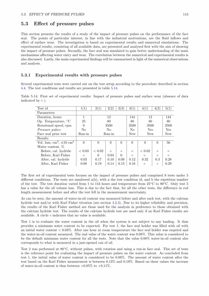
5.3. EFFECT OF PRESSURE PULSES 113
5.3 Effect of pressure pulses
This section presents the results of a study of the impact of pressure pulses on the performance of the faceseal. The points of particular interest, in line with the industrial motivations, are the fluid inflows andeffect of surface wear. The investigation is based on experimental results and numerical simulations. Theexperimental results, consisting of all available data, are presented and analysed first with the aim of showingthe impact of pressure pulses. Secondly, the face seal was simulated to gain better understanding of the mainmechanisms affecting water entry and wear. The correlation between the numerical and experimental results isalso discussed. Lastly, the main experimental findings will be summarised in light of the numerical observationsand analysis.
5.3.1 Experimental results with pressure pulses
Several experimental tests were carried out on the test setup according to the procedure described in section4.4. The test conditions and results are presented in table 5.14.
Table 5.14: First set of experimental results: Impact of pressure pulses and surface wear (absence of dataindicated by ).
Test id 1(1) 2(1) 2(2) 2(3) 3(1) 4(1) 4(2) 5(1)ParametersDuration, hours 1 12 144 12 144Op. Temperature, C 25 80 80 80 80Rotational speed, rpm 0 3500 3500 3500 3500Pressure pulses No No No Yes YesFace seal prior test Run-in Run-in New New NewResultsVol. loss, cm3, ±10 cm3 0 0 0 0 0 0 0 56Water content, %
Before, cal. hydride < 0.03 < 0.02 < 0.02 Before, Karl Fisher 0 0.04 0 After, cal. hydride 0.03 0.17 0.10 0.09 0.12 0.32 0.3 0.28After, Karl Fisher 0.08 0.19 0.14 0.13 0.16 0.29
The first set of experimental tests focuses on the impact of pressure pulses and comprised 8 tests under 5different conditions. The tests are numbered a(b), with a the test condition id, and b the repetition numberof the test. The test duration varied from 1 to 144 hours and temperature from 25C to 80C. Only test 5has a value for the oil volume loss. This is due to the fact that, for all the other tests, the difference in rodlength measurement before and after the test fell in the measurement uncertainty.
As can be seen, the amount of water-in-oil content was measured before and after each test, with the calciumhydride test and/or with Karl Fisher titration (see section 4.2.3). Due to its higher reliability and precision,the results of the Karl Fisher method are those used for the analysis in preference to those obtained withthe calcium hydride test. The results of the calcium hydride test are used only if no Karl Fisher results areavailable. A circle indicates that no value is available.
Test 1 is to evaluate the water content in the oil when the system is not subject to any loading. It thusprovides a minimum water content to be expected. For test 1, the face seal holder was filled with oil withan initial water content < 0.03%. After one hour at room temperature the face seal holder was emptied andthe water-in-oil content measured. The end value of the water content was 0.08%. This value is considered tobe the default minimum water content for all the tests. Note that the value 0.08% water-in-oil content alsocorresponds to what is measured in a just-opened can of oil.
Test 2 was performed at 80C, without pulses, with rotation and using a run-in face seal. This set of testsis the reference point for evaluating the impact of pressure pulses on the water content. As concluded fromtest 1, the initial value of water content is considered to be 0.08%. The amount of water content after thetest based on the Karl Fisher measurement is between 0.13% and 0.19%. Based on these values the increaseof water-in-oil content is thus between +0.05% to +0.11%.
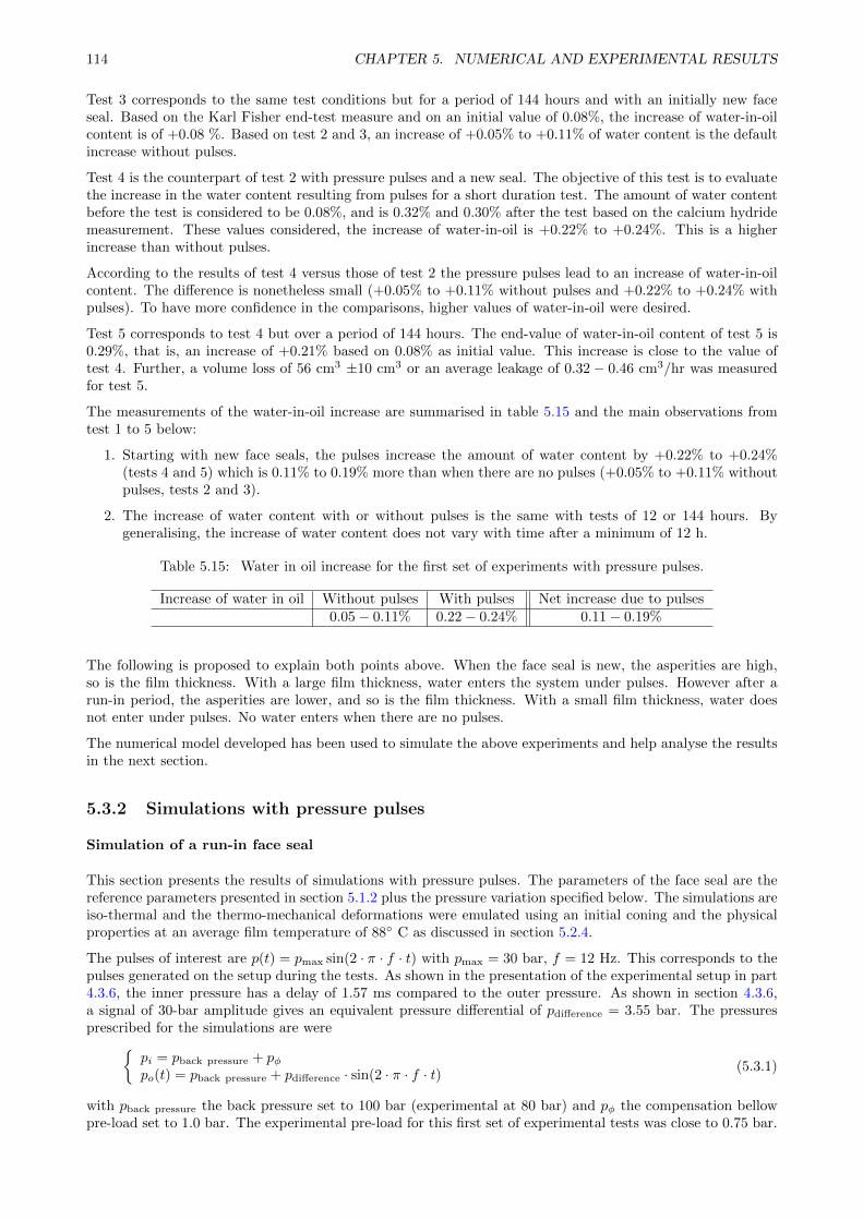
114 CHAPTER 5. NUMERICAL AND EXPERIMENTAL RESULTS
Test 3 corresponds to the same test conditions but for a period of 144 hours and with an initially new faceseal. Based on the Karl Fisher end-test measure and on an initial value of 0.08%, the increase of water-in-oilcontent is of +0.08 %. Based on test 2 and 3, an increase of +0.05% to +0.11% of water content is the defaultincrease without pulses.
Test 4 is the counterpart of test 2 with pressure pulses and a new seal. The objective of this test is to evaluatethe increase in the water content resulting from pulses for a short duration test. The amount of water contentbefore the test is considered to be 0.08%, and is 0.32% and 0.30% after the test based on the calcium hydridemeasurement. These values considered, the increase of water-in-oil is +0.22% to +0.24%. This is a higherincrease than without pulses.
According to the results of test 4 versus those of test 2 the pressure pulses lead to an increase of water-in-oilcontent. The difference is nonetheless small (+0.05% to +0.11% without pulses and +0.22% to +0.24% withpulses). To have more confidence in the comparisons, higher values of water-in-oil were desired.
Test 5 corresponds to test 4 but over a period of 144 hours. The end-value of water-in-oil content of test 5 is0.29%, that is, an increase of +0.21% based on 0.08% as initial value. This increase is close to the value oftest 4. Further, a volume loss of 56 cm3 ±10 cm3 or an average leakage of 0.32− 0.46 cm3/hr was measuredfor test 5.
The measurements of the water-in-oil increase are summarised in table 5.15 and the main observations fromtest 1 to 5 below:
1. Starting with new face seals, the pulses increase the amount of water content by +0.22% to +0.24%(tests 4 and 5) which is 0.11% to 0.19% more than when there are no pulses (+0.05% to +0.11% withoutpulses, tests 2 and 3).
2. The increase of water content with or without pulses is the same with tests of 12 or 144 hours. Bygeneralising, the increase of water content does not vary with time after a minimum of 12 h.
Table 5.15: Water in oil increase for the first set of experiments with pressure pulses.
Increase of water in oil Without pulses With pulses Net increase due to pulses0.05− 0.11% 0.22− 0.24% 0.11− 0.19%
The following is proposed to explain both points above. When the face seal is new, the asperities are high,so is the film thickness. With a large film thickness, water enters the system under pulses. However after arun-in period, the asperities are lower, and so is the film thickness. With a small film thickness, water doesnot enter under pulses. No water enters when there are no pulses.
The numerical model developed has been used to simulate the above experiments and help analyse the resultsin the next section.
5.3.2 Simulations with pressure pulses
Simulation of a run-in face seal
This section presents the results of simulations with pressure pulses. The parameters of the face seal are thereference parameters presented in section 5.1.2 plus the pressure variation specified below. The simulations areiso-thermal and the thermo-mechanical deformations were emulated using an initial coning and the physicalproperties at an average film temperature of 88 C as discussed in section 5.2.4.
The pulses of interest are p(t) = pmax sin(2 · π · f · t) with pmax = 30 bar, f = 12 Hz. This corresponds to thepulses generated on the setup during the tests. As shown in the presentation of the experimental setup in part4.3.6, the inner pressure has a delay of 1.57 ms compared to the outer pressure. As shown in section 4.3.6,a signal of 30-bar amplitude gives an equivalent pressure differential of pdifference = 3.55 bar. The pressuresprescribed for the simulations are were
pi = pback pressure + pφpo(t) = pback pressure + pdifference · sin(2 · π · f · t) (5.3.1)
with pback pressure the back pressure set to 100 bar (experimental at 80 bar) and pφ the compensation bellowpre-load set to 1.0 bar. The experimental pre-load for this first set of experimental tests was close to 0.75 bar.
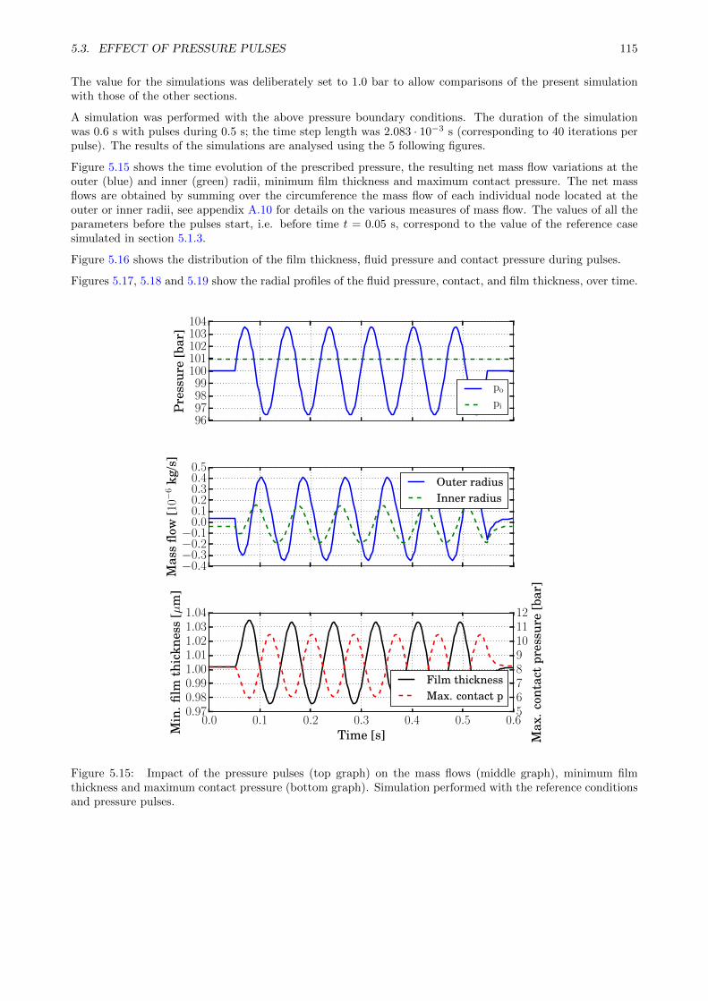
5.3. EFFECT OF PRESSURE PULSES 115
The value for the simulations was deliberately set to 1.0 bar to allow comparisons of the present simulationwith those of the other sections.
A simulation was performed with the above pressure boundary conditions. The duration of the simulationwas 0.6 s with pulses during 0.5 s; the time step length was 2.083 · 10−3 s (corresponding to 40 iterations perpulse). The results of the simulations are analysed using the 5 following figures.
Figure 5.15 shows the time evolution of the prescribed pressure, the resulting net mass flow variations at theouter (blue) and inner (green) radii, minimum film thickness and maximum contact pressure. The net massflows are obtained by summing over the circumference the mass flow of each individual node located at theouter or inner radii, see appendix A.10 for details on the various measures of mass flow. The values of all theparameters before the pulses start, i.e. before time t = 0.05 s, correspond to the value of the reference casesimulated in section 5.1.3.
Figure 5.16 shows the distribution of the film thickness, fluid pressure and contact pressure during pulses.
Figures 5.17, 5.18 and 5.19 show the radial profiles of the fluid pressure, contact, and film thickness, over time.
96979899
100101102103104
Pre
ssur
e[b
ar]
po
pi
−0.4−0.3−0.2−0.1
0.00.10.20.30.40.5
Mas
sflo
w[1
0−6
kg/s
]
Outer radiusInner radius
0.0 0.1 0.2 0.3 0.4 0.5 0.6Time [s]
0.970.980.991.001.011.021.031.04
Min
.film
thic
knes
s[µ
m]
56789101112
Max
.con
tact
pres
sure
[bar
]
Film thicknessMax. contact p
Figure 5.15: Impact of the pressure pulses (top graph) on the mass flows (middle graph), minimum filmthickness and maximum contact pressure (bottom graph). Simulation performed with the reference conditionsand pressure pulses.
116 CHAPTER 5. NUMERICAL AND EXPERIMENTAL RESULTS
A1 B1
t =
0.0
70
83
st
= 0
.09
16
7 s
t =
0.1
12
5 s
t =
0.1
33
3 s
A2
A3
A4
B2
B3
B4
C1
C2
C3
C4
Figure 5.16: Evolution of the film thickness (left), fluid pressure (middle) and contact pressure (right) of thereference face seal during pressure pulses.
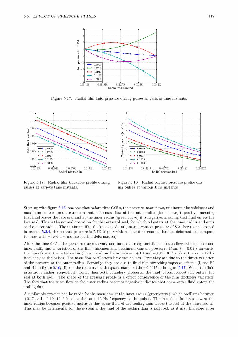
5.3. EFFECT OF PRESSURE PULSES 117
0.011138 0.011919 0.012700 0.013481 0.014262Radial position [m]
−4
−3
−2
−1
0
1
2
3
4
Flu
idpr
essu
re[x
105
Pa]
0.05000.07080.09170.11250.1333
Figure 5.17: Radial film fluid pressure during pulses at various time instants.
0.011138 0.011919 0.012700 0.013481 0.014262Radial position [m]
0.98
1.00
1.02
1.04
1.06
1.08
1.10
1.12
Film
thic
knes
s[µ
m]
0.05000.07080.09170.11250.1333
Figure 5.18: Radial film thickness profile duringpulses at various time instants.
0.011138 0.011919 0.012700 0.013481 0.014262Radial position [m]
2
3
4
5
6
7
8
9
10
11
Con
tact
pres
sure
[x10
5P
a]
0.05000.07080.09170.11250.1333
Figure 5.19: Radial contact pressure profile dur-ing pulses at various time instants.
Starting with figure 5.15, one sees that before time 0.05 s, the pressure, mass flows, minimum film thickness andmaximum contact pressure are constant. The mass flow at the outer radius (blue curve) is positive, meaningthat fluid leaves the face seal and at the inner radius (green curve) it is negative, meaning that fluid enters theface seal. This is the normal operation for this outward seal, for which oil enters at the inner radius and exitsat the outer radius. The minimum film thickness is of 1.00 µm and contact pressure of 8.21 bar (as mentionedin section 5.2.4, the contact pressure is 7.5% higher with emulated thermo-mechanical deformations compareto cases with solved thermo-mechanical deformation).
After the time 0.05 s the pressure starts to vary and induces strong variations of mass flows at the outer andinner radii, and a variation of the film thickness and maximum contact pressure. From t = 0.05 s onwards,the mass flow at the outer radius (blue curve) oscillates between +0.4 and −0.33 ·10−6 kg/s at the same 12 Hzfrequency as the pulses. The mass flow oscillations have two causes. First they are due to the direct variationof the pressure at the outer radius. Secondly, they are due to fluid film stretching/squeeze effects: (i) see B2and B4 in figure 5.16; (ii) see the red curve with square markers (time 0.0917 s) in figure 5.17. When the fluidpressure is higher, respectively lower, than both boundary pressures, the fluid leaves, respectively enters, theseal at both radii. The shape of the pressure profile is a direct consequence of the film thickness variation.The fact that the mass flow at the outer radius becomes negative indicates that some outer fluid enters thesealing dam.
A similar observation can be made for the mass flow at the inner radius (green curve), which oscillates between+0.17 and −0.19 · 10−6 kg/s at the same 12-Hz frequency as the pulses. The fact that the mass flow at theinner radius becomes positive indicates that some fluid of the sealing dam leaves the seal at the inner radius.This may be detrimental for the system if the fluid of the sealing dam is polluted, as it may therefore enter
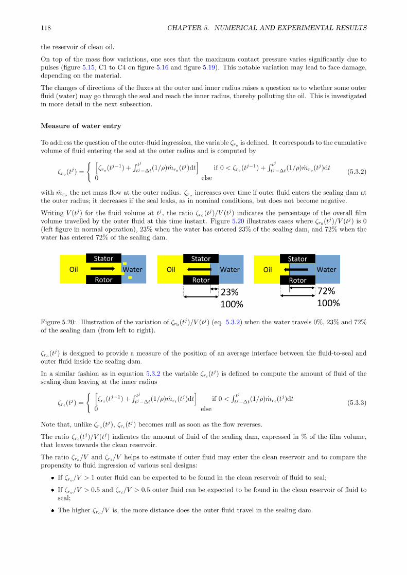
118 CHAPTER 5. NUMERICAL AND EXPERIMENTAL RESULTS
the reservoir of clean oil.
On top of the mass flow variations, one sees that the maximum contact pressure varies significantly due topulses (figure 5.15, C1 to C4 on figure 5.16 and figure 5.19). This notable variation may lead to face damage,depending on the material.
The changes of directions of the fluxes at the outer and inner radius raises a question as to whether some outerfluid (water) may go through the seal and reach the inner radius, thereby polluting the oil. This is investigatedin more detail in the next subsection.
Measure of water entry
To address the question of the outer-fluid ingression, the variable ζro is defined. It corresponds to the cumulativevolume of fluid entering the seal at the outer radius and is computed by
ζro(tj) =
[ζro(tj−1) +
∫ tjtj−∆t
(1/ρ)mro(tj)dt]
if 0 < ζro(tj−1) +∫ tjtj−∆t
(1/ρ)mro(tj)dt
0 else(5.3.2)
with mro the net mass flow at the outer radius. ζro increases over time if outer fluid enters the sealing dam atthe outer radius; it decreases if the seal leaks, as in nominal conditions, but does not become negative.
Writing V (tj) for the fluid volume at tj , the ratio ζr0(tj)/V (tj) indicates the percentage of the overall filmvolume travelled by the outer fluid at this time instant. Figure 5.20 illustrates cases where ζr0(tj)/V (tj) is 0(left figure in normal operation), 23% when the water has entered 23% of the sealing dam, and 72% when thewater has entered 72% of the sealing dam.
WaterOil
Stator
Rotor
100%23%
WaterOil
Stator
Rotor
WaterOil
Stator
Rotor
100%72%
Figure 5.20: Illustration of the variation of ζr0(tj)/V (tj) (eq. 5.3.2) when the water travels 0%, 23% and 72%of the sealing dam (from left to right).
ζro(tj) is designed to provide a measure of the position of an average interface between the fluid-to-seal andouter fluid inside the sealing dam.
In a similar fashion as in equation 5.3.2 the variable ζri(tj) is defined to compute the amount of fluid of the
sealing dam leaving at the inner radius
ζri(tj) =
[ζri(t
j−1) +∫ tjtj−∆t
(1/ρ)mri(tj)dt
]if 0 <
∫ tjtj−∆t
(1/ρ)mri(tj)dt
0 else(5.3.3)
Note that, unlike ζro(tj), ζri(tj) becomes null as soon as the flow reverses.
The ratio ζri(tj)/V (tj) indicates the amount of fluid of the sealing dam, expressed in % of the film volume,
that leaves towards the clean reservoir.
The ratio ζro/V and ζri/V helps to estimate if outer fluid may enter the clean reservoir and to compare thepropensity to fluid ingression of various seal designs:
If ζro/V > 1 outer fluid can be expected to be found in the clean reservoir of fluid to seal;
If ζro/V > 0.5 and ζri/V > 0.5 outer fluid can be expected to be found in the clean reservoir of fluid toseal;
The higher ζro/V is, the more distance does the outer fluid travel in the sealing dam.
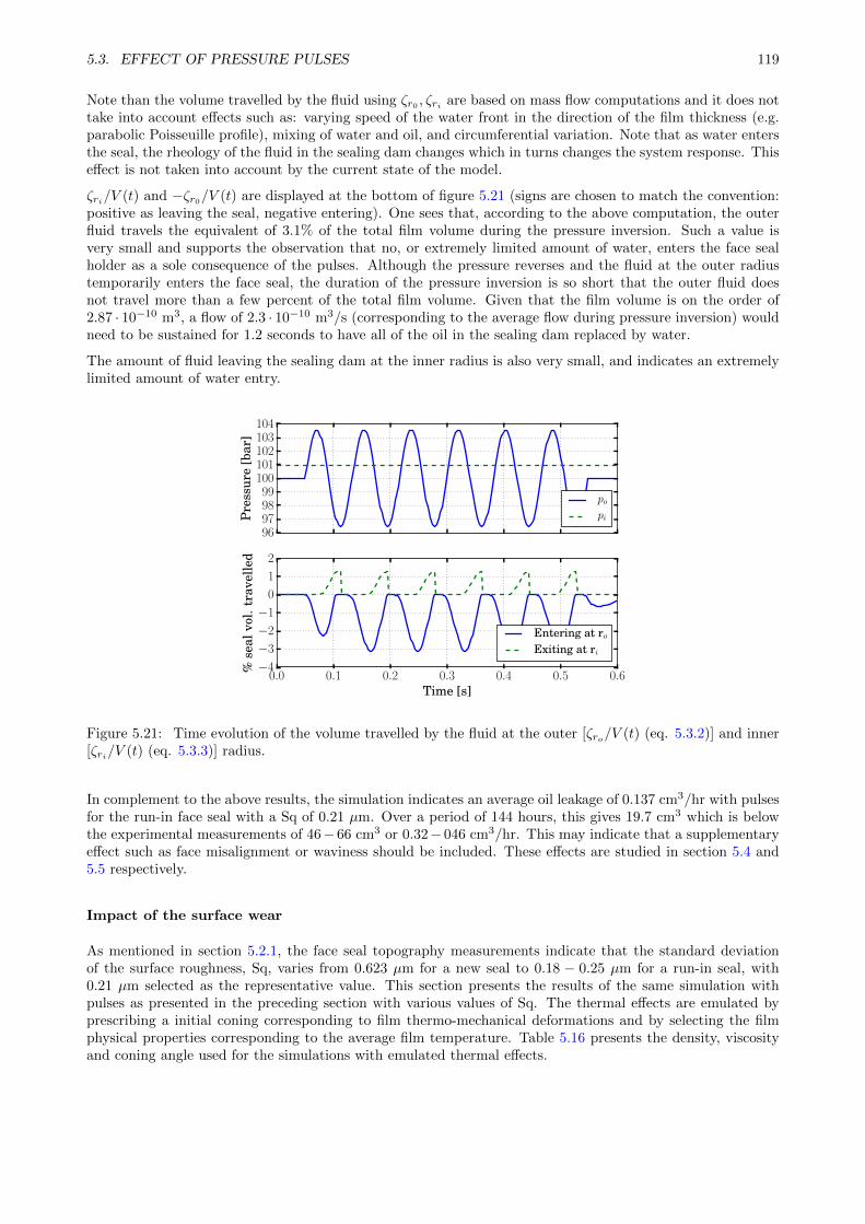
5.3. EFFECT OF PRESSURE PULSES 119
Note than the volume travelled by the fluid using ζr0 , ζri are based on mass flow computations and it does nottake into account effects such as: varying speed of the water front in the direction of the film thickness (e.g.parabolic Poisseuille profile), mixing of water and oil, and circumferential variation. Note that as water entersthe seal, the rheology of the fluid in the sealing dam changes which in turns changes the system response. Thiseffect is not taken into account by the current state of the model.
ζri/V (t) and −ζr0/V (t) are displayed at the bottom of figure 5.21 (signs are chosen to match the convention:positive as leaving the seal, negative entering). One sees that, according to the above computation, the outerfluid travels the equivalent of 3.1% of the total film volume during the pressure inversion. Such a value isvery small and supports the observation that no, or extremely limited amount of water, enters the face sealholder as a sole consequence of the pulses. Although the pressure reverses and the fluid at the outer radiustemporarily enters the face seal, the duration of the pressure inversion is so short that the outer fluid doesnot travel more than a few percent of the total film volume. Given that the film volume is on the order of2.87 · 10−10 m3, a flow of 2.3 · 10−10 m3/s (corresponding to the average flow during pressure inversion) wouldneed to be sustained for 1.2 seconds to have all of the oil in the sealing dam replaced by water.
The amount of fluid leaving the sealing dam at the inner radius is also very small, and indicates an extremelylimited amount of water entry.
96979899
100101102103104
Pre
ssur
e[b
ar]
po
pi
0.0 0.1 0.2 0.3 0.4 0.5 0.6Time [s]
−4
−3
−2
−1
0
1
2
%se
alvo
l.tr
avel
led
Entering at roExiting at ri
Figure 5.21: Time evolution of the volume travelled by the fluid at the outer [ζro/V (t) (eq. 5.3.2)] and inner[ζri/V (t) (eq. 5.3.3)] radius.
In complement to the above results, the simulation indicates an average oil leakage of 0.137 cm3/hr with pulsesfor the run-in face seal with a Sq of 0.21 µm. Over a period of 144 hours, this gives 19.7 cm3 which is belowthe experimental measurements of 46− 66 cm3 or 0.32− 046 cm3/hr. This may indicate that a supplementaryeffect such as face misalignment or waviness should be included. These effects are studied in section 5.4 and5.5 respectively.
Impact of the surface wear
As mentioned in section 5.2.1, the face seal topography measurements indicate that the standard deviationof the surface roughness, Sq, varies from 0.623 µm for a new seal to 0.18 − 0.25 µm for a run-in seal, with0.21 µm selected as the representative value. This section presents the results of the same simulation withpulses as presented in the preceding section with various values of Sq. The thermal effects are emulated byprescribing a initial coning corresponding to film thermo-mechanical deformations and by selecting the filmphysical properties corresponding to the average film temperature. Table 5.16 presents the density, viscosityand coning angle used for the simulations with emulated thermal effects.
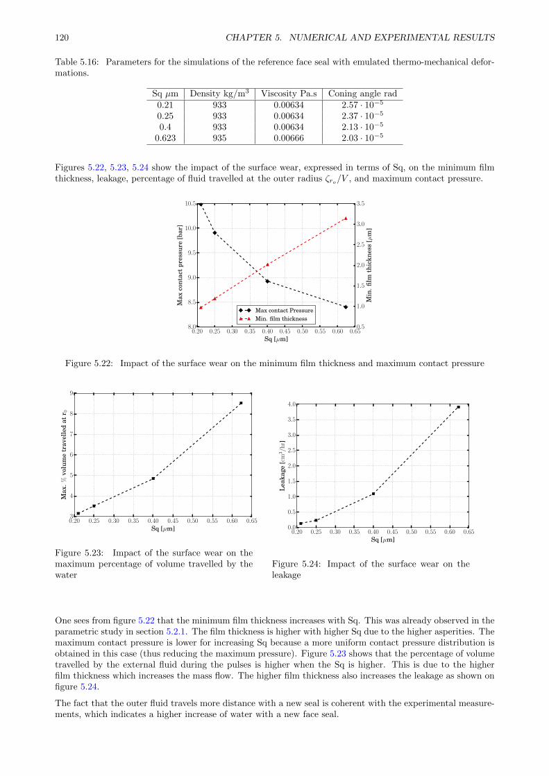
120 CHAPTER 5. NUMERICAL AND EXPERIMENTAL RESULTS
Table 5.16: Parameters for the simulations of the reference face seal with emulated thermo-mechanical defor-mations.
Sq µm Density kg/m3 Viscosity Pa.s Coning angle rad0.21 933 0.00634 2.57 · 10−5
0.25 933 0.00634 2.37 · 10−5
0.4 933 0.00634 2.13 · 10−5
0.623 935 0.00666 2.03 · 10−5
Figures 5.22, 5.23, 5.24 show the impact of the surface wear, expressed in terms of Sq, on the minimum filmthickness, leakage, percentage of fluid travelled at the outer radius ζro/V , and maximum contact pressure.
0.20 0.25 0.30 0.35 0.40 0.45 0.50 0.55 0.60 0.65Sq [µm]
8.0
8.5
9.0
9.5
10.0
10.5
Max
cont
act
pres
sure
[bar
]
0.5
1.0
1.5
2.0
2.5
3.0
3.5
Min
.film
thic
knes
s[µ
m]
Max contact PressureMin. film thickness
Figure 5.22: Impact of the surface wear on the minimum film thickness and maximum contact pressure
0.20 0.25 0.30 0.35 0.40 0.45 0.50 0.55 0.60 0.65Sq [µm]
3
4
5
6
7
8
9
Max
.%vo
lum
etr
avel
led
atr 0
Figure 5.23: Impact of the surface wear on themaximum percentage of volume travelled by thewater
0.20 0.25 0.30 0.35 0.40 0.45 0.50 0.55 0.60 0.65Sq [µm]
0.0
0.5
1.0
1.5
2.0
2.5
3.0
3.5
4.0
Lea
kage
[cm
3/h
r]
Figure 5.24: Impact of the surface wear on theleakage
One sees from figure 5.22 that the minimum film thickness increases with Sq. This was already observed in theparametric study in section 5.2.1. The film thickness is higher with higher Sq due to the higher asperities. Themaximum contact pressure is lower for increasing Sq because a more uniform contact pressure distribution isobtained in this case (thus reducing the maximum pressure). Figure 5.23 shows that the percentage of volumetravelled by the external fluid during the pulses is higher when the Sq is higher. This is due to the higherfilm thickness which increases the mass flow. The higher film thickness also increases the leakage as shown onfigure 5.24.
The fact that the outer fluid travels more distance with a new seal is coherent with the experimental measure-ments, which indicates a higher increase of water with a new face seal.
5.3. EFFECT OF PRESSURE PULSES 121
5.3.3 Conclusions from the study of pressure pulses
This section presented an experimental and numerical study of the impact of pressure pulses and pressureinversion on the face seal of interest. As shown by the experimental results, when a new face seal with 1.0 barover pressure is subject to pulses of ±3.55 bar at 12 Hz:
The pulses increase the amount of water content in the oil by +0.22% to +0.24% (tests 4 and 5) whichis 0.11% to 0.19% more than when there are no pulses (+0.05% to +0.11% without pulses, tests 2 and3);
The increase of water content in oil, with or without pulses, is the same with tests of 12 or 144 hours.By generalising, the increase of water content does not vary with time after a minimum of 12 h.
The water entry is larger with a new face seal operating under pulses and does not increase proportionallywith time. This can be explained by the fact that water enters only when the seal in not run-in, as it has ahigher film thickness. When the surfaces are run-in, the film thickness is lower and does not allow water toenter. This is supported by the simulation results done for face seals with various levels of wear, characterisedby the Sq of the face (see figure 5.22). When considering a new face seal, typically Sq = 0.623 µm, the outerfluid travels 10% of the film volume compared to 3.3% for a run-in seal of Sq = 0.21 µm.
The volume loss predicted by the simulation over a period of 144 h is of 19.7 cm3 which is lower than the46− 66 cm3 measured for test 5. Supplementary effects such as face misalignment or face waviness may haveto be included in the simulations and are investigated in the subsequent sections.
The new face seals also have lower maximum contact pressure. This can be understood by looking at thecontact equation (equation 4 in section 2.2.4) and observing the variation of contact pressure as a function ofboth Sq and Sq/h.
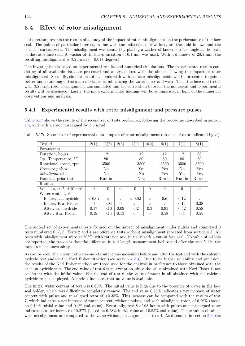
122 CHAPTER 5. NUMERICAL AND EXPERIMENTAL RESULTS
5.4 Effect of rotor misalignment
This section presents the results of a study of the impact of rotor misalignment on the performance of the faceseal. The points of particular interest, in line with the industrial motivations, are the fluid inflows and theeffect of surface wear. The misalignment was created by placing a washer of known surface angle at the backof the rotor face seal. A washer of thickness variation of 0.1 mm was used. With a diameter of 28.5 mm, theresulting misalignment is 3.5 mrad (= 0.017 degrees).
The investigation is based on experimental results and numerical simulations. The experimental results con-sisting of all available data are presented and analysed first with the aim of showing the impact of rotormisalignment. Secondly, simulations of face seals with various rotor misalignments will be presented to gain abetter understanding of the main mechanisms influencing the water entry and wear. Then the face seal testedwith 3.5 mrad rotor misalignment was simulated and the correlation between the numerical and experimentalresults will be discussed. Lastly, the main experimental findings will be summarised in light of the numericalobservations and analysis.
5.4.1 Experimental results with rotor misalignment and pressure pulses
Table 5.17 shows the results of the second set of tests performed, following the procedure described in section4.4, and with a rotor misaligned by 3.5 mrad
Table 5.17: Second set of experimental data: Impact of rotor misalignment (absence of data indicated by ).
Test id 2(1) 2(2) 2(3) 4(1) 4(2) 6(1) 7(1) 8(1)ParametersDuration, hours 12 12 12 12 68Op. Temperature, C 80 80 80 80 80Rotational speed, rpm 3500 3500 3500 3500 3500Pressure pulses No Yes Yes No YesMisalignment No No Yes Yes YesFace seal prior test Run-in New Run-in Run-in Run-inResultsVol. loss, cm3, ±10 cm3 0 0 0 0 0 0 0 0Water content, %
Before, cal. hydride < 0.02 < 0.02 0.6 0.12 Before, Karl Fisher 0 0.04 0 0.14 0.28After, cal. hydride 0.17 0.10 0.09 0.32 0.3 0.95 0.42 0.58After, Karl Fisher 0.19 0.14 0.13 0.58 0.4 0.55
The second set of experimental tests focused on the impact of misalignment under pulses and comprised 3tests numbered 6, 7, 8. Tests 2 and 4 are reference tests without misalignment repeated from section 5.3. Alltests with misalignment were at 80C, with rotation and initially with a run-in face seal. No value of oil lossare reported, the reason is that the difference in rod length measurement before and after the test fell in themeasurement uncertainty.
As can be seen, the amount of water-in-oil content was measured before and after the test and with the calciumhydride test and/or the Karl Fisher titration (see section 4.2.3). Due to its higher reliability and precision,the results of the Karl Fisher method are those used for the analysis in preference to those obtained with thecalcium hydride test. The end value of test 6 is an exception, since the value obtained with Karl Fisher is notconsistent with the initial value. For the end of test 6, the value of water in oil obtained with the calciumhydride test is employed. A circle indicates that no value is available.
The initial water content of test 6 is 0.60%. The initial value is high due to the presence of water in the faceseal holder, which was difficult to completely remove. The end value 0.95% indicates a net increase of watercontent with pulses and misaligned rotor of +0.35%. This increase can be compared with the results of test7, which indicates a net increase of water content, without pulses, and with misaligned rotor, of 0.26% (basedon 0.14% initial value and 0.4% end-value). Eventually, test 8 of 68 hours with pulses and misaligned rotorindicates a water increase of 0.27% (based on 0.28% initial value and 0.55% end-value). These values obtainedwith misalignment are compared to the value without misalignment of test 4. As discussed in section 5.3, the
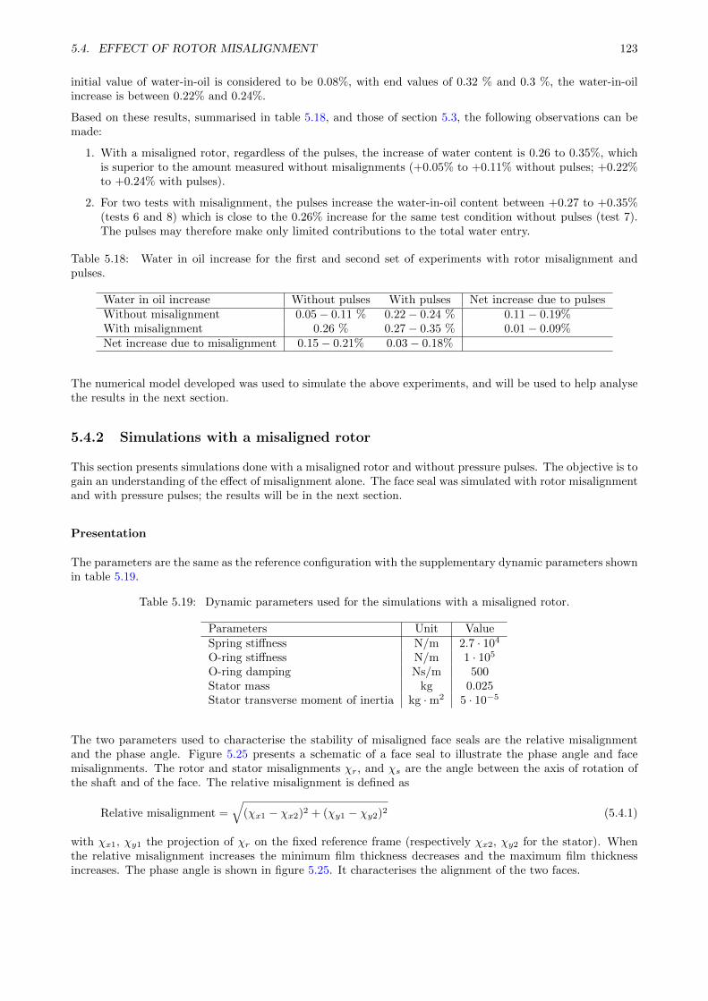
5.4. EFFECT OF ROTOR MISALIGNMENT 123
initial value of water-in-oil is considered to be 0.08%, with end values of 0.32 % and 0.3 %, the water-in-oilincrease is between 0.22% and 0.24%.
Based on these results, summarised in table 5.18, and those of section 5.3, the following observations can bemade:
1. With a misaligned rotor, regardless of the pulses, the increase of water content is 0.26 to 0.35%, whichis superior to the amount measured without misalignments (+0.05% to +0.11% without pulses; +0.22%to +0.24% with pulses).
2. For two tests with misalignment, the pulses increase the water-in-oil content between +0.27 to +0.35%(tests 6 and 8) which is close to the 0.26% increase for the same test condition without pulses (test 7).The pulses may therefore make only limited contributions to the total water entry.
Table 5.18: Water in oil increase for the first and second set of experiments with rotor misalignment andpulses.
Water in oil increase Without pulses With pulses Net increase due to pulsesWithout misalignment 0.05− 0.11 % 0.22− 0.24 % 0.11− 0.19%With misalignment 0.26 % 0.27− 0.35 % 0.01− 0.09%Net increase due to misalignment 0.15− 0.21% 0.03− 0.18%
The numerical model developed was used to simulate the above experiments, and will be used to help analysethe results in the next section.
5.4.2 Simulations with a misaligned rotor
This section presents simulations done with a misaligned rotor and without pressure pulses. The objective is togain an understanding of the effect of misalignment alone. The face seal was simulated with rotor misalignmentand with pressure pulses; the results will be in the next section.
Presentation
The parameters are the same as the reference configuration with the supplementary dynamic parameters shownin table 5.19.
Table 5.19: Dynamic parameters used for the simulations with a misaligned rotor.
Parameters Unit ValueSpring stiffness N/m 2.7 · 104
O-ring stiffness N/m 1 · 105
O-ring damping Ns/m 500Stator mass kg 0.025Stator transverse moment of inertia kg ·m2 5 · 10−5
The two parameters used to characterise the stability of misaligned face seals are the relative misalignmentand the phase angle. Figure 5.25 presents a schematic of a face seal to illustrate the phase angle and facemisalignments. The rotor and stator misalignments χr, and χs are the angle between the axis of rotation ofthe shaft and of the face. The relative misalignment is defined as
Relative misalignment =√
(χx1 − χx2)2 + (χy1 − χy2)2 (5.4.1)
with χx1, χy1 the projection of χr on the fixed reference frame (respectively χx2, χy2 for the stator). Whenthe relative misalignment increases the minimum film thickness decreases and the maximum film thicknessincreases. The phase angle is shown in figure 5.25. It characterises the alignment of the two faces.
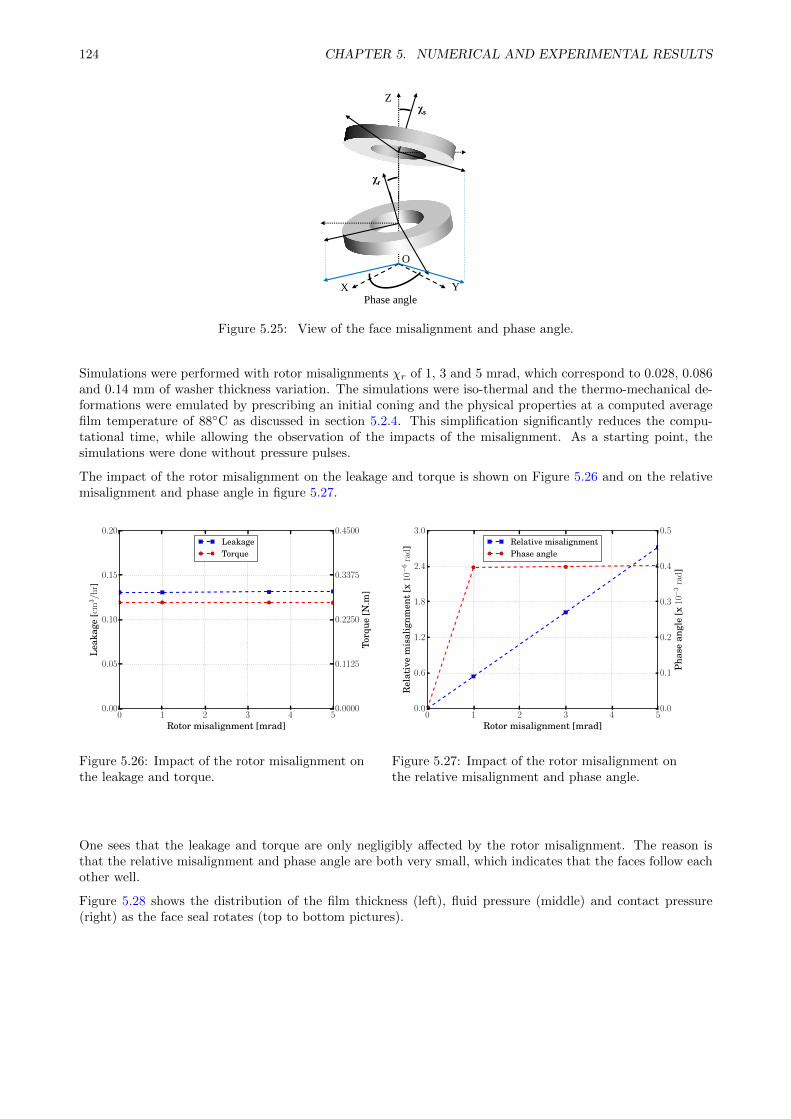
124 CHAPTER 5. NUMERICAL AND EXPERIMENTAL RESULTS
χr
χs
X Y
Z
O
Phase angle
Figure 5.25: View of the face misalignment and phase angle.
Simulations were performed with rotor misalignments χr of 1, 3 and 5 mrad, which correspond to 0.028, 0.086and 0.14 mm of washer thickness variation. The simulations were iso-thermal and the thermo-mechanical de-formations were emulated by prescribing an initial coning and the physical properties at a computed averagefilm temperature of 88C as discussed in section 5.2.4. This simplification significantly reduces the compu-tational time, while allowing the observation of the impacts of the misalignment. As a starting point, thesimulations were done without pressure pulses.
The impact of the rotor misalignment on the leakage and torque is shown on Figure 5.26 and on the relativemisalignment and phase angle in figure 5.27.
0 1 2 3 4 5Rotor misalignment [mrad]
0.00
0.05
0.10
0.15
0.20
Lea
kage
[cm
3/h
r]
LeakageTorque
0.0000
0.1125
0.2250
0.3375
0.4500
Torq
ue[N
.m]
Figure 5.26: Impact of the rotor misalignment onthe leakage and torque.
0 1 2 3 4 5Rotor misalignment [mrad]
0.0
0.6
1.2
1.8
2.4
3.0
Rel
ativ
em
isal
ignm
ent
[x10−
6ra
d] Relative misalignment
Phase angle
0.0
0.1
0.2
0.3
0.4
0.5
Pha
sean
gle
[x10−
3ra
d]
Figure 5.27: Impact of the rotor misalignment onthe relative misalignment and phase angle.
One sees that the leakage and torque are only negligibly affected by the rotor misalignment. The reason isthat the relative misalignment and phase angle are both very small, which indicates that the faces follow eachother well.
Figure 5.28 shows the distribution of the film thickness (left), fluid pressure (middle) and contact pressure(right) as the face seal rotates (top to bottom pictures).
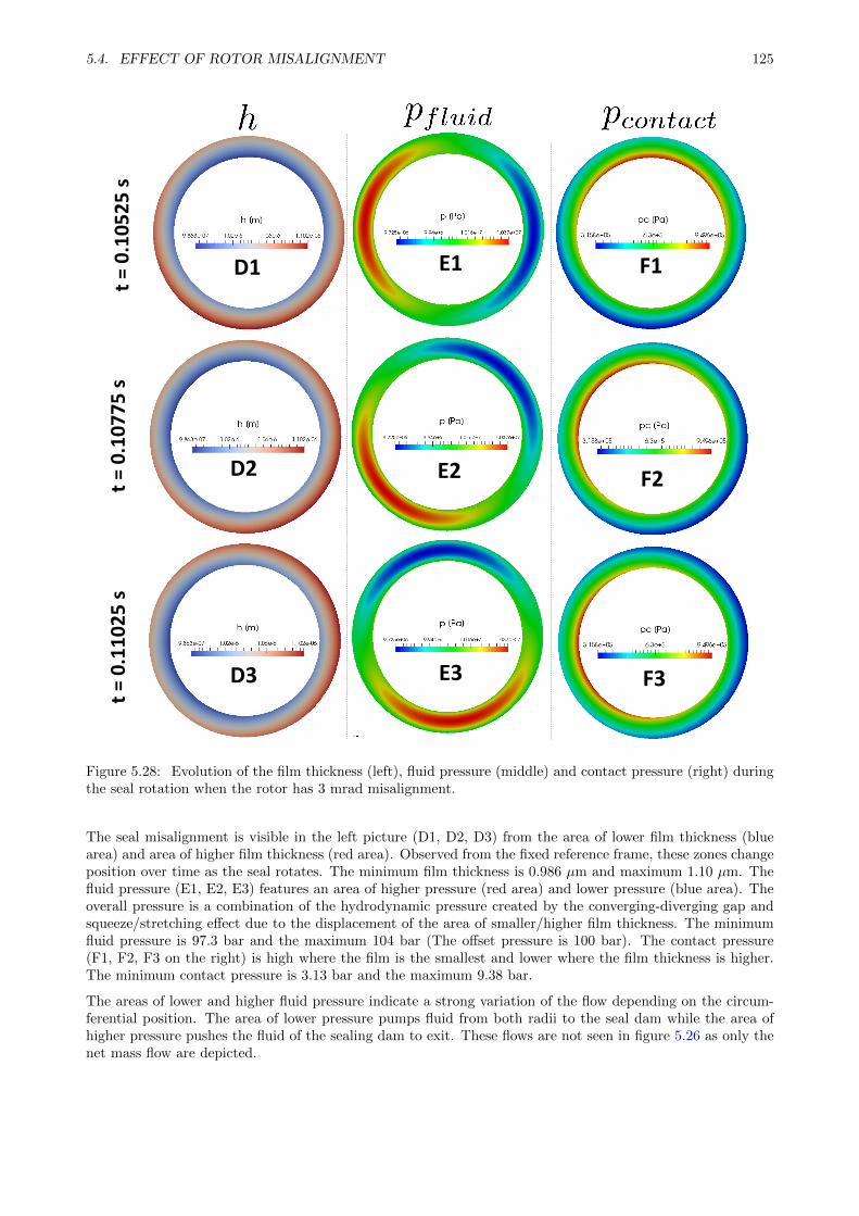
5.4. EFFECT OF ROTOR MISALIGNMENT 125
D1 E1
t =
0.1
05
25
st
= 0
.10
77
5 s
t =
0.1
10
25
s
D2
D3
E2
E3
F1
F2
F3
Figure 5.28: Evolution of the film thickness (left), fluid pressure (middle) and contact pressure (right) duringthe seal rotation when the rotor has 3 mrad misalignment.
The seal misalignment is visible in the left picture (D1, D2, D3) from the area of lower film thickness (bluearea) and area of higher film thickness (red area). Observed from the fixed reference frame, these zones changeposition over time as the seal rotates. The minimum film thickness is 0.986 µm and maximum 1.10 µm. Thefluid pressure (E1, E2, E3) features an area of higher pressure (red area) and lower pressure (blue area). Theoverall pressure is a combination of the hydrodynamic pressure created by the converging-diverging gap andsqueeze/stretching effect due to the displacement of the area of smaller/higher film thickness. The minimumfluid pressure is 97.3 bar and the maximum 104 bar (The offset pressure is 100 bar). The contact pressure(F1, F2, F3 on the right) is high where the film is the smallest and lower where the film thickness is higher.The minimum contact pressure is 3.13 bar and the maximum 9.38 bar.
The areas of lower and higher fluid pressure indicate a strong variation of the flow depending on the circum-ferential position. The area of lower pressure pumps fluid from both radii to the seal dam while the area ofhigher pressure pushes the fluid of the sealing dam to exit. These flows are not seen in figure 5.26 as only thenet mass flow are depicted.
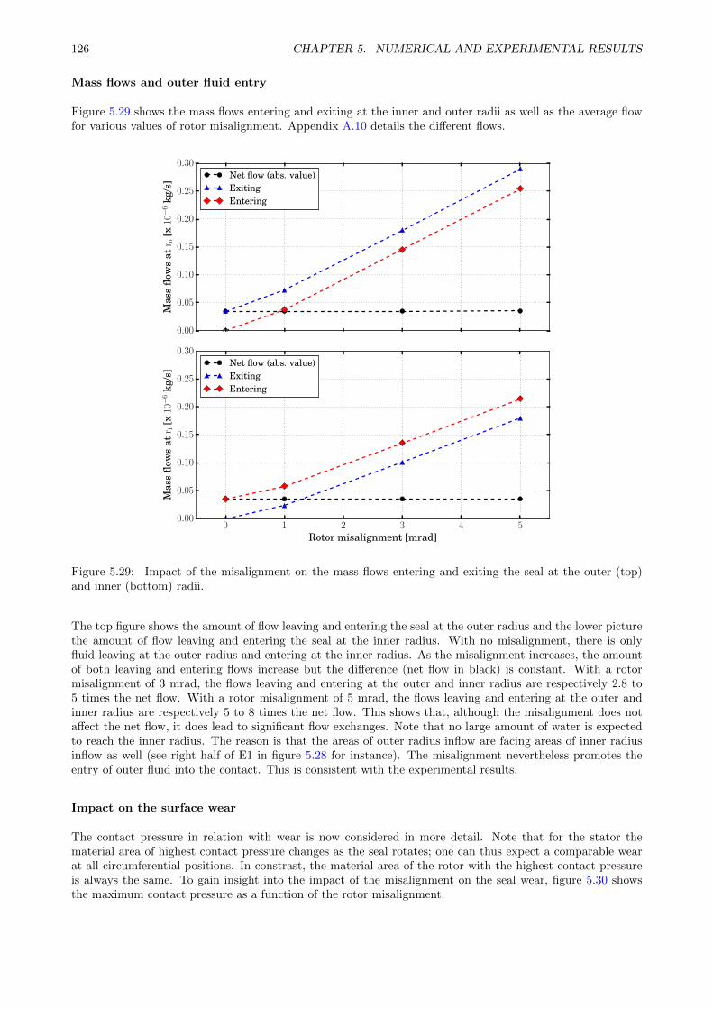
126 CHAPTER 5. NUMERICAL AND EXPERIMENTAL RESULTS
Mass flows and outer fluid entry
Figure 5.29 shows the mass flows entering and exiting at the inner and outer radii as well as the average flowfor various values of rotor misalignment. Appendix A.10 details the different flows.
0.00
0.05
0.10
0.15
0.20
0.25
0.30M
ass
flow
sat
r o[x
10−
6kg
/s] Net flow (abs. value)
ExitingEntering
0 1 2 3 4 5Rotor misalignment [mrad]
0.00
0.05
0.10
0.15
0.20
0.25
0.30
Mas
sflo
ws
atr i
[x10−
6kg
/s]
Net flow (abs. value)ExitingEntering
Figure 5.29: Impact of the misalignment on the mass flows entering and exiting the seal at the outer (top)and inner (bottom) radii.
The top figure shows the amount of flow leaving and entering the seal at the outer radius and the lower picturethe amount of flow leaving and entering the seal at the inner radius. With no misalignment, there is onlyfluid leaving at the outer radius and entering at the inner radius. As the misalignment increases, the amountof both leaving and entering flows increase but the difference (net flow in black) is constant. With a rotormisalignment of 3 mrad, the flows leaving and entering at the outer and inner radius are respectively 2.8 to5 times the net flow. With a rotor misalignment of 5 mrad, the flows leaving and entering at the outer andinner radius are respectively 5 to 8 times the net flow. This shows that, although the misalignment does notaffect the net flow, it does lead to significant flow exchanges. Note that no large amount of water is expectedto reach the inner radius. The reason is that the areas of outer radius inflow are facing areas of inner radiusinflow as well (see right half of E1 in figure 5.28 for instance). The misalignment nevertheless promotes theentry of outer fluid into the contact. This is consistent with the experimental results.
Impact on the surface wear
The contact pressure in relation with wear is now considered in more detail. Note that for the stator thematerial area of highest contact pressure changes as the seal rotates; one can thus expect a comparable wearat all circumferential positions. In constrast, the material area of the rotor with the highest contact pressureis always the same. To gain insight into the impact of the misalignment on the seal wear, figure 5.30 showsthe maximum contact pressure as a function of the rotor misalignment.
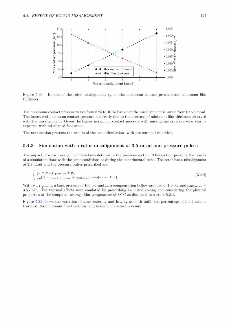
5.4. EFFECT OF ROTOR MISALIGNMENT 127
0 1 2 3 4 5Rotor misalignment [mrad]
8.0
8.5
9.0
9.5
10.0
10.5
11.0
Max
cont
act
pres
sure
[bar
]
0.970
0.975
0.980
0.985
0.990
0.995
1.000
1.005
Min
.film
thic
knes
s[µ
m]
Max contact PressureMin. film thickness
Figure 5.30: Impact of the rotor misalignment χr on the maximum contact pressure and minimum filmthickness.
The maximum contact pressure varies from 8.25 to 10.75 bar when the misalignment is varied from 0 to 5 mrad.The increase of maximum contact pressure is directly due to the decrease of minimum film thickness observedwith the misalignment. Given the higher maximum contact pressure with misalignments, more wear can beexpected with misaligned face seals.
The next section presents the results of the same simulations with pressure pulses added.
5.4.3 Simulation with a rotor misalignment of 3.5 mrad and pressure pulses
The impact of rotor misalignment has been detailed in the previous section. This section presents the resultsof a simulation done with the same conditions as during the experimental tests. The rotor has a misalignmentof 3.5 mrad and the pressure pulses prescribed are
pi = pback pressure + pφpo(t) = pback pressure + pdifference · sin(2 · π · f · t) (5.4.2)
With pback pressure a back pressure of 100 bar and pφ a compensation bellow pre-load of 1.0 bar and pdifference =3.55 bar. The thermal effects were emulated by prescribing an initial coning and considering the physicalproperties at the computed average film temperature of 88C as discussed in section 5.2.4.
Figure 5.31 shows the variation of mass entering and leaving at both radii, the percentage of fluid volumetravelled, the minimum film thickness, and maximum contact pressure.
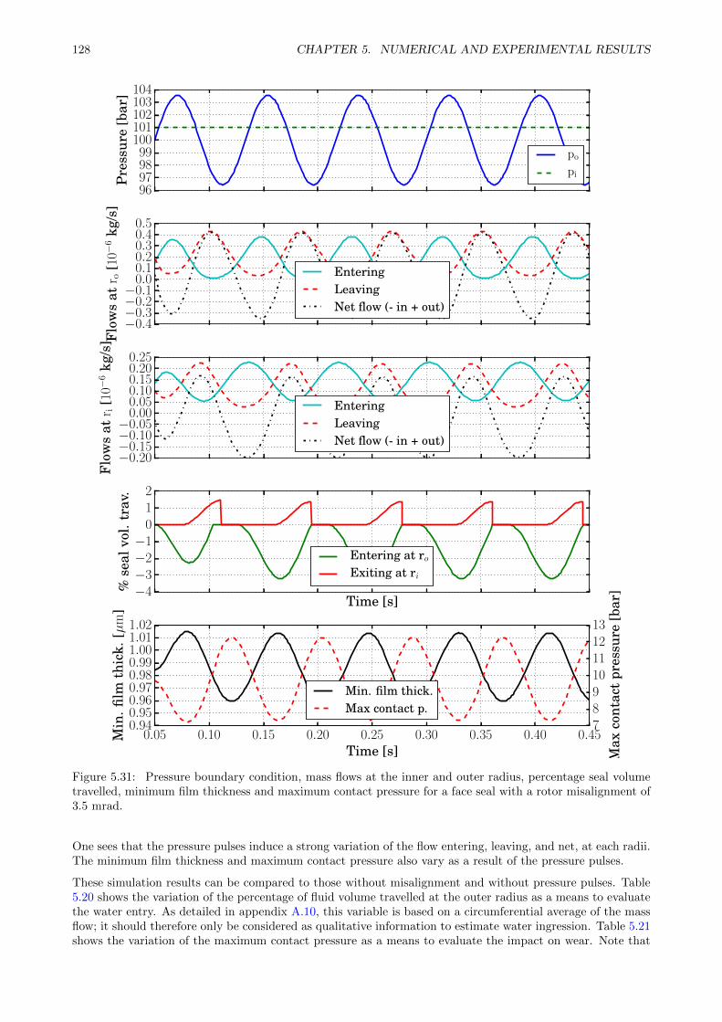
128 CHAPTER 5. NUMERICAL AND EXPERIMENTAL RESULTS
96979899
100101102103104
Pre
ssur
e[b
ar]
po
pi
−0.4−0.3−0.2−0.1
0.00.10.20.30.40.5
Flo
ws
atr o
[10−
6kg
/s]
EnteringLeavingNet flow (- in + out)
−0.20−0.15−0.10−0.05
0.000.050.100.150.200.25
Flo
ws
atr i
[10−
6kg
/s]
EnteringLeavingNet flow (- in + out)
Time [s]−4−3−2−1
012
%se
alvo
l.tr
av.
Entering at roExiting at ri
0.05 0.10 0.15 0.20 0.25 0.30 0.35 0.40 0.45Time [s]
0.940.950.960.970.980.991.001.011.02
Min
.film
thic
k.[µ
m]
78910111213
Max
cont
act
pres
sure
[bar
]
Min. film thick.Max contact p.
Figure 5.31: Pressure boundary condition, mass flows at the inner and outer radius, percentage seal volumetravelled, minimum film thickness and maximum contact pressure for a face seal with a rotor misalignment of3.5 mrad.
One sees that the pressure pulses induce a strong variation of the flow entering, leaving, and net, at each radii.The minimum film thickness and maximum contact pressure also vary as a result of the pressure pulses.
These simulation results can be compared to those without misalignment and without pressure pulses. Table5.20 shows the variation of the percentage of fluid volume travelled at the outer radius as a means to evaluatethe water entry. As detailed in appendix A.10, this variable is based on a circumferential average of the massflow; it should therefore only be considered as qualitative information to estimate water ingression. Table 5.21shows the variation of the maximum contact pressure as a means to evaluate the impact on wear. Note that
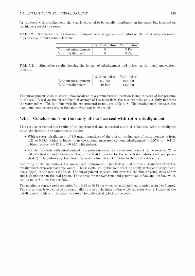
5.4. EFFECT OF ROTOR MISALIGNMENT 129
for the cases with misalignment, the wear is expected to be equally distributed on the stator but localised onthe higher spot for the rotor.
Table 5.20: Simulation results showing the impact of misalignment and pulses on the water entry expressedin percentage of fluid volume travelled.
Without pulses With pulsesWithout misalignment 0 3.1%With misalignment 0 3.3%
Table 5.21: Simulation results showing the impact of misalignment and pulses on the maximum contactpressure.
Without pulses With pulsesWithout misalignment 8.2 bar 10.5 barWith misalignment 10 bar 12.2 bar
The misalignment leads to water inflow localised in a circumferential position facing the area of low pressurein the seal. Based on the circumferential average of the mass flow, the misalignment only slightly increasesthe water inflow. This is in line with the experimental results, see table 5.18. The misalignment increases themaximum contact pressure, so that more wear can be expected.
5.4.4 Conclusions from the study of the face seal with rotor misalignment
This section presented the results of an experimental and numerical study of a face seal with a misalignedrotor. As shown by the experimental results:
With a rotor misalignment of 3.5 mrad, regardless of the pulses, the increase of water content is from0.26 to 0.35%, which is higher than the amount measured without misalignment (+0.05% to +0.11%without pulses; +0.22% to +0.24% with pulses).
For the two tests with misalignment, the pulses increase the water-in-oil content by between +0.27 to+0.35% (tests 6 and 8) which is close to the 0.26% increase for the same test conditions without pulses(test 7). The pulses may therefore only make a limited contribution to the total water entry.
According to the simulations, the overall seal performance - net leakage and torque - is unaffected by themisalignment even when of large values. This is explained by the good tracking ability (relative misalignment,phase angle) of the face seal tested. The misalignment squeezes and stretches the film, creating areas of lowand high pressure in the seal region. These areas rotate over time and generate an inflow and outflow whichcan be up to 8 times the net flow.
The maximum contact pressure varies from 8.25 to 10.75 bar when the misalignment is varied from 0 to 5 mrad.The stator wear is expected to be equally distributed at the inner radius while the rotor wear is located at themisalignment. This will ultimately create a circumferential defect in the rotor.
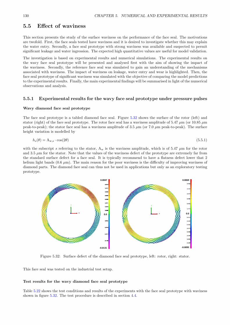
130 CHAPTER 5. NUMERICAL AND EXPERIMENTAL RESULTS
5.5 Effect of waviness
This section presents the study of the surface waviness on the performance of the face seal. The motivationsare twofold. First, the face seals tested have waviness and it is desired to investigate whether this may explainthe water entry. Secondly, a face seal prototype with strong waviness was available and suspected to permitsignificant leakage and water ingression. The expected high quantitative values are useful for model validation.
The investigation is based on experimental results and numerical simulations. The experimental results onthe wavy face seal prototype will be presented and analysed first with the aim of showing the impact ofthe waviness. Secondly, the reference face seal was simulated to gain an understanding of the mechanismsassociated with waviness. The impact of waviness on leakage, water entry and wear is highlighted. Then, theface seal prototype of significant waviness was simulated with the objective of comparing the model predictionsto the experimental results. Finally, the main experimental findings will be summarised in light of the numericalobservations and analysis.
5.5.1 Experimental results for the wavy face seal prototype under pressure pulses
Wavy diamond face seal prototype
The face seal prototype is a tabled diamond face seal. Figure 5.32 shows the surface of the rotor (left) andstator (right) of the face seal prototype. The rotor face seal has a waviness amplitude of 5.47 µm (or 10.85 µmpeak-to-peak); the stator face seal has a waviness amplitude of 3.5 µm (or 7.0 µm peak-to-peak). The surfaceheight variation is modelled by
hs(θ) = Aw,s · cos(2θ) (5.5.1)
with the subscript s referring to the stator, Aw is the waviness amplitude, which is of 5.47 µm for the rotorand 3.5 µm for the stator. Note that the values of the waviness defect of the prototype are extremely far fromthe standard surface defect for a face seal. It is typically recommend to have a flatness defect lower that 2helium light bands (0.6 µm). The main reason for the poor waviness is the difficulty of improving waviness ofdiamond parts. The diamond face seal can thus not be used in applications but only as an exploratory testingprototype.
0.0047
-0.0131
0.0
-0.0095
0.0069
0.0
Figure 5.32: Surface defect of the diamond face seal prototype, left: rotor, right: stator.
This face seal was tested on the industrial test setup.
Test results for the wavy diamond face seal prototype
Table 5.22 shows the test conditions and results of the experiments with the face seal prototype with wavinessshown in figure 5.32. The test procedure is described in section 4.4.
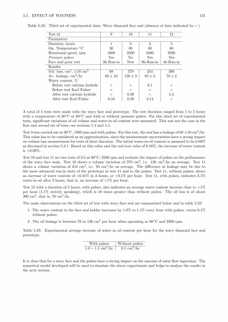
5.5. EFFECT OF WAVINESS 131
Table 5.22: Third set of experimental data: Wavy diamond face seal (absence of data indicated by ).
Test id 9 10 11 12ParametersDuration, hours 1 3 3 5Op. Temperature C 30 80 80 80Rotational speed, rpm 1000 3500 3500 3500Pressure pulses Yes No Yes YesFace seal prior test 3h-Run-in New 9h-Run-in 4h-Run-inResultsVol. loss, cm3, ±10 cm3 68 379 254 390Av. leakage, cm3/hr 68± 10 126± 3 85± 3 78± 2Water content, %
Before test calcium hydride 0.1 Before test Karl Fisher After test calcium hydride 0.39 5.5After test Karl Fisher 0.16 0.39 3.14
A total of 4 tests were made with the wavy face seal prototype. The test duration ranged from 1 to 5 hourswith a temperature of 30C or 80C and with or without pressure pulses. For this third set of experimentaltests, significant variations of oil volume and water-in-oil content were measured. This was not the case in thefirst and second set of tests, see sections 5.3 and 5.4.
Test 9 was carried out at 30C, 1000 rpm and with pulses. For this test, the seal has a leakage of 68 ±10 cm3/hr.This value has to be considered as an approximation, since the measurement uncertainties have a strong impacton volume loss measurement for tests of short duration. The initial water-in-oil content is assumed to be 0.08%as discussed in section 5.3.1. Based on this value and the end-test value of 0.16%, the increase of water contentis +0.08%.
Test 10 and test 11 are two tests of 3 h at 80C, 3500 rpm and evaluate the impact of pulses on the performanceof the wavy face seals. Test 10 shows a volume variation of 379 cm3, i.e. 126 cm3/hr on average. Test 11shows a volume variation of 254 cm3, i.e. 85 cm3/hr on average. The difference in leakage may be due tothe more advanced run-in state of the prototype in test 11 and to the pulses. Test 11, without pulses, showsan increase of water content of +0.31% in 3 hours, or +0.1% per hour. Test 11, with pulses, indicates 3.1%water-in-oil after 3 hours, that is, an increase of +1% per hour.
Test 12 with a duration of 5 hours, with pulses, also indicates an average water content increase close to +1%per hour (1.1% strictly speaking), which is 10 times greater than without pulses. The oil loss is of about390 cm3, that is, 78 cm3/hr.
The main observations on the third set of test with wavy face seal are summarised below and in table 5.23:
1. The water content in the face seal holder increases by 1.0% to 1.1% every hour with pulses, versus 0.1%without pulses.
2. The oil leakage is between 78 to 126 cm3 per hour when operating at 80C and 3500 rpm.
Table 5.23: Experimental average increase of water in oil content per hour for the wavy diamond face sealprototype.
With pulses Without pulses1.0− 1.1 cm3/hr 0.1 cm3/hr
It is clear that for a wavy face seal the pulses have a strong impact on the amount of outer flow ingression. Thenumerical model developed will be used to simulate the above experiments and helps to analyse the results inthe next section.
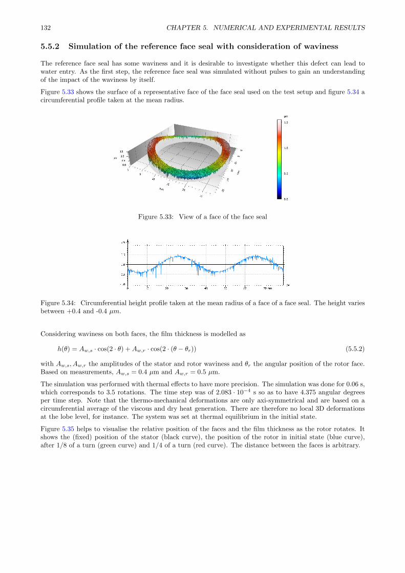
132 CHAPTER 5. NUMERICAL AND EXPERIMENTAL RESULTS
5.5.2 Simulation of the reference face seal with consideration of waviness
The reference face seal has some waviness and it is desirable to investigate whether this defect can lead towater entry. As the first step, the reference face seal was simulated without pulses to gain an understandingof the impact of the waviness by itself.
Figure 5.33 shows the surface of a representative face of the face seal used on the test setup and figure 5.34 acircumferential profile taken at the mean radius.
Figure 5.33: View of a face of the face seal
Figure 5.34: Circumferential height profile taken at the mean radius of a face of a face seal. The height variesbetween +0.4 and -0.4 µm.
Considering waviness on both faces, the film thickness is modelled as
h(θ) = Aw,s · cos(2 · θ) +Aw,r · cos(2 · (θ − θr)) (5.5.2)
with Aw,s, Aw,r the amplitudes of the stator and rotor waviness and θr the angular position of the rotor face.Based on measurements, Aw,s = 0.4 µm and Aw,r = 0.5 µm.
The simulation was performed with thermal effects to have more precision. The simulation was done for 0.06 s,which corresponds to 3.5 rotations. The time step was of 2.083 · 10−4 s so as to have 4.375 angular degreesper time step. Note that the thermo-mechanical deformations are only axi-symmetrical and are based on acircumferential average of the viscous and dry heat generation. There are therefore no local 3D deformationsat the lobe level, for instance. The system was set at thermal equilibrium in the initial state.
Figure 5.35 helps to visualise the relative position of the faces and the film thickness as the rotor rotates. Itshows the (fixed) position of the stator (black curve), the position of the rotor in initial state (blue curve),after 1/8 of a turn (green curve) and 1/4 of a turn (red curve). The distance between the faces is arbitrary.
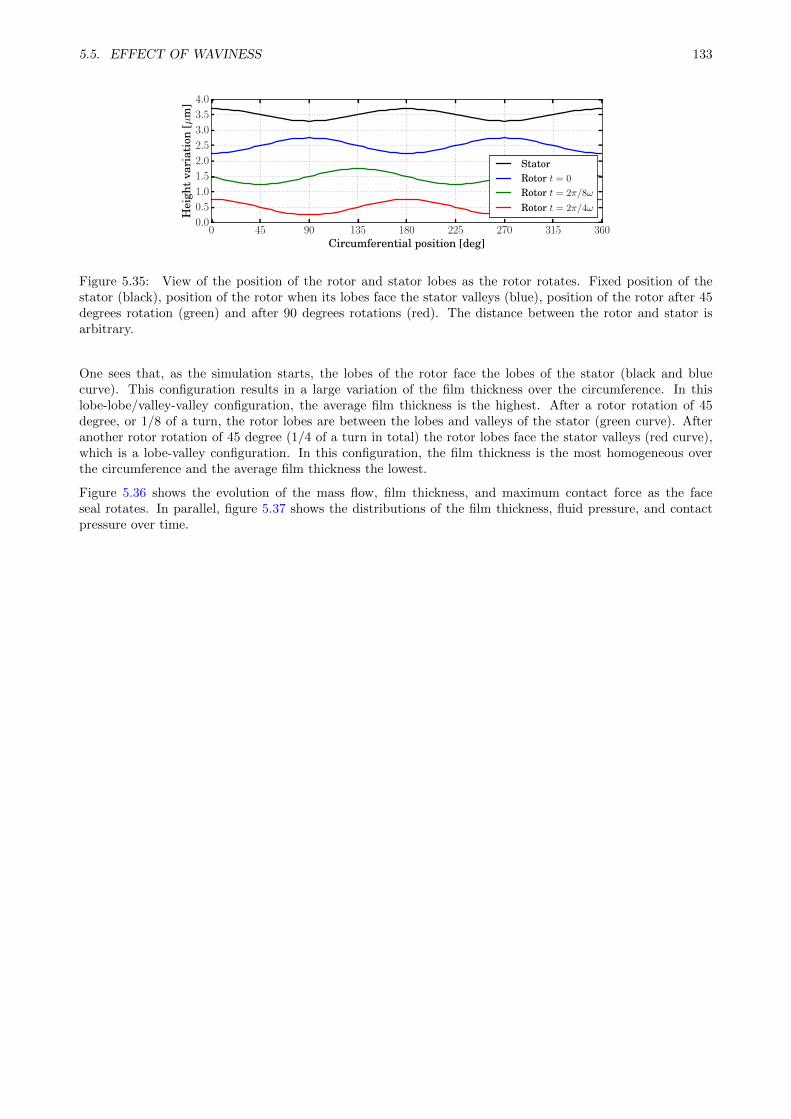
5.5. EFFECT OF WAVINESS 133
0 45 90 135 180 225 270 315 360Circumferential position [deg]
0.0
0.5
1.0
1.5
2.0
2.5
3.0
3.5
4.0
Hei
ght
vari
atio
n[µ
m]
StatorRotor t = 0
Rotor t = 2π/8ω
Rotor t = 2π/4ω
Figure 5.35: View of the position of the rotor and stator lobes as the rotor rotates. Fixed position of thestator (black), position of the rotor when its lobes face the stator valleys (blue), position of the rotor after 45degrees rotation (green) and after 90 degrees rotations (red). The distance between the rotor and stator isarbitrary.
One sees that, as the simulation starts, the lobes of the rotor face the lobes of the stator (black and bluecurve). This configuration results in a large variation of the film thickness over the circumference. In thislobe-lobe/valley-valley configuration, the average film thickness is the highest. After a rotor rotation of 45degree, or 1/8 of a turn, the rotor lobes are between the lobes and valleys of the stator (green curve). Afteranother rotor rotation of 45 degree (1/4 of a turn in total) the rotor lobes face the stator valleys (red curve),which is a lobe-valley configuration. In this configuration, the film thickness is the most homogeneous overthe circumference and the average film thickness the lowest.
Figure 5.36 shows the evolution of the mass flow, film thickness, and maximum contact force as the faceseal rotates. In parallel, figure 5.37 shows the distributions of the film thickness, fluid pressure, and contactpressure over time.
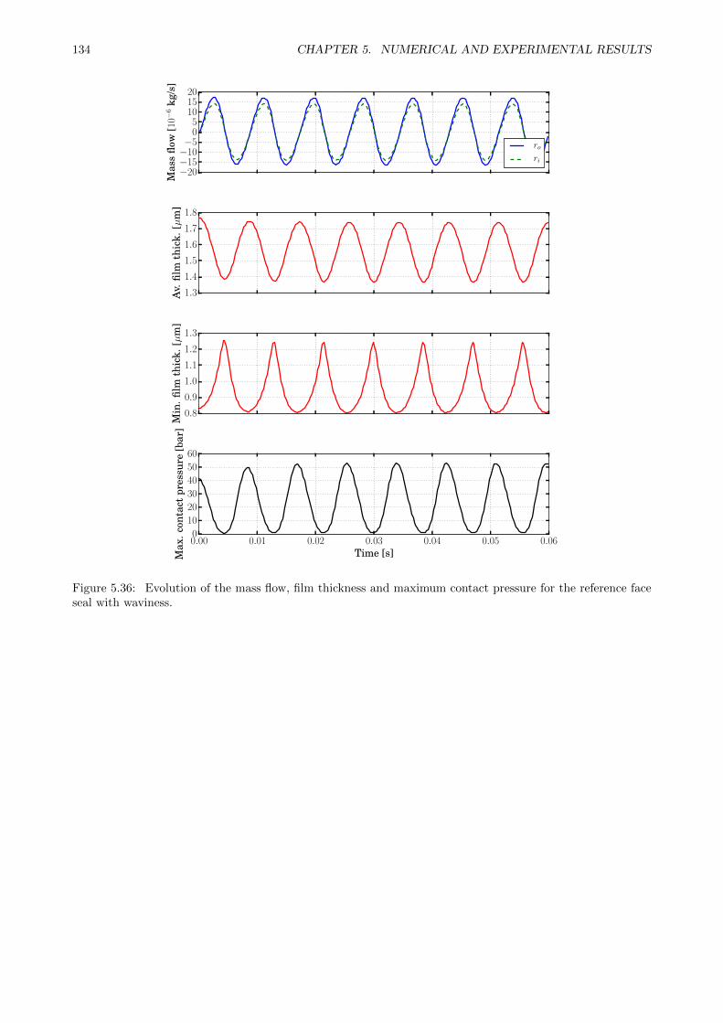
134 CHAPTER 5. NUMERICAL AND EXPERIMENTAL RESULTS
−20−15−10−5
05
101520
Mas
sflo
w[1
0−6
kg/s
]
ro
ri
1.3
1.4
1.5
1.6
1.7
1.8
Av.
film
thic
k.[µ
m]
0.8
0.9
1.0
1.1
1.2
1.3
Min
.film
thic
k.[µ
m]
0.00 0.01 0.02 0.03 0.04 0.05 0.06Time [s]
0
10
20
30
40
50
60
Max
.con
tact
pres
sure
[bar
]
Figure 5.36: Evolution of the mass flow, film thickness and maximum contact pressure for the reference faceseal with waviness.
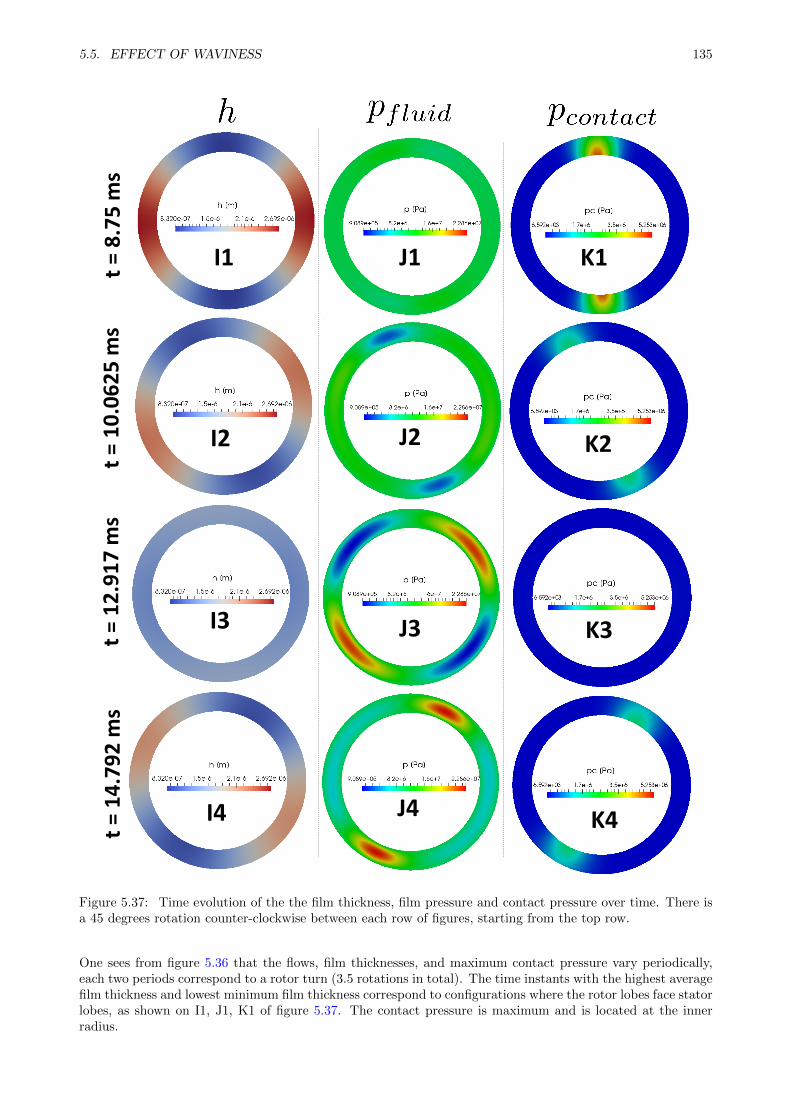
5.5. EFFECT OF WAVINESS 135
I1 J1
t =
8.7
5 m
st
= 1
0.0
62
5 m
st
= 1
2.9
17
ms
t =
14
.79
2 m
s
I2
I3
I4
J2
J3
J4
K1
K2
K3
K4
Figure 5.37: Time evolution of the the film thickness, film pressure and contact pressure over time. There isa 45 degrees rotation counter-clockwise between each row of figures, starting from the top row.
One sees from figure 5.36 that the flows, film thicknesses, and maximum contact pressure vary periodically,each two periods correspond to a rotor turn (3.5 rotations in total). The time instants with the highest averagefilm thickness and lowest minimum film thickness correspond to configurations where the rotor lobes face statorlobes, as shown on I1, J1, K1 of figure 5.37. The contact pressure is maximum and is located at the innerradius.
136 CHAPTER 5. NUMERICAL AND EXPERIMENTAL RESULTS
As the rotor rotates, the lobes move to the stator valley (time 8.75 ms to 12.917 ms). The average filmthickness diminishes, the minimum film thickness increases, and maximum contact pressure diminishes. Ascan be seen from the top graph of figure 5.36, this phase is associated with positive mass flow, that is, fluidleaving at both radii. As seen in J2 from figure 5.37, areas of higher and lower pressure exist at the sametime in the film. The subsequent configuration depicted in J3 is a lobe-valley. In this case the average filmthickness is minimum, the minimum film thickness maximum, the maximum contact pressure minimum, andthe fluid stops leaving. The system moves then from a lobe-valley to lobe-lobe configuration during which theaverage film thickness increases, minimum film thickness decreases, maximum contact pressure increases. Themass flows are negative, indicating that the fluid enters the seal at both radii during this phase.
The rotor lobes are then facing the stator lobes, as in the initial configuration. Overall, the instantaneousmass flows vary between 17 to −16 · 10−6 kg/s. Figure 5.36 also shows that the maximum contact pressurevaries significantly, from 50 bar in lobe-lobe configuration to 0 bar in lobe-valley configuration.
The next sections will investigate the impact of the waviness on the mass flow and wear through the maximumcontact pressure in more detail.
Mass flows variations
As shown in figure 5.38 below, the net flows at each radius are composed of inflows and outflows varying in time.This is due to the complex pressure profile depicted in figure 5.37. The inflows take place at the circumferentialpositions facing areas of low pressure in the film and the outflows at the circumferential positions facing areasof high pressure in the film.
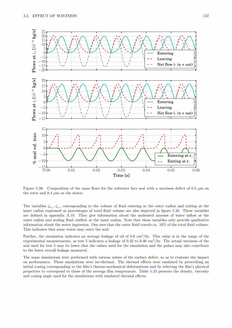
5.5. EFFECT OF WAVINESS 137
−20−15−10−5
05
10152025
Flo
ws
atr o
[10−
6kg
/s]
EnteringLeavingNet flow (- in + out)
−15−10−5
05
101520
Flo
ws
atr i
[10−
6kg
/s]
EnteringLeavingNet flow (- in + out)
0.00 0.01 0.02 0.03 0.04 0.05 0.06Time [s]
−15
−10
−5
0
5
10
15
%se
alvo
l.tr
av.
Entering at roExiting at ri
Figure 5.38: Composition of the mass flows for the reference face seal with a waviness defect of 0.5 µm onthe rotor and 0.4 µm on the stator.
The variables ζro , ζri , corresponding to the volume of fluid entering at the outer radius and exiting at theinner radius expressed as percentages of total fluid volume are also depicted in figure 5.38. These variablesare defined in appendix A.10. They give information about the undesired amount of water inflow at theouter radius and sealing fluid outflow at the inner radius. Note that these variables only provide qualitativeinformation about the water ingression. One sees that the outer fluid travels ca. 10% of the total fluid volume.This indicates that some water may enter the seal.
Further, the simulation indicates an average leakage of oil of 0.6 cm3/hr. This value is in the range of theexperimental measurements, as test 5 indicates a leakage of 0.32 to 0.46 cm3/hr. The actual waviness of theseal used for test 5 may be lower that the values used for the simulation and the pulses may also contributeto the lower overall leakage measured.
The same simulations were performed with various values of the surface defect, so as to evaluate the impacton performance. These simulations were iso-thermal. The thermal effects were emulated by prescribing aninitial coning corresponding to the film’s thermo-mechanical deformations and by selecting the film’s physicalproperties to correspond to those of the average film temperature. Table 5.24 presents the density, viscosityand coning angle used for the simulations with emulated thermal effects.
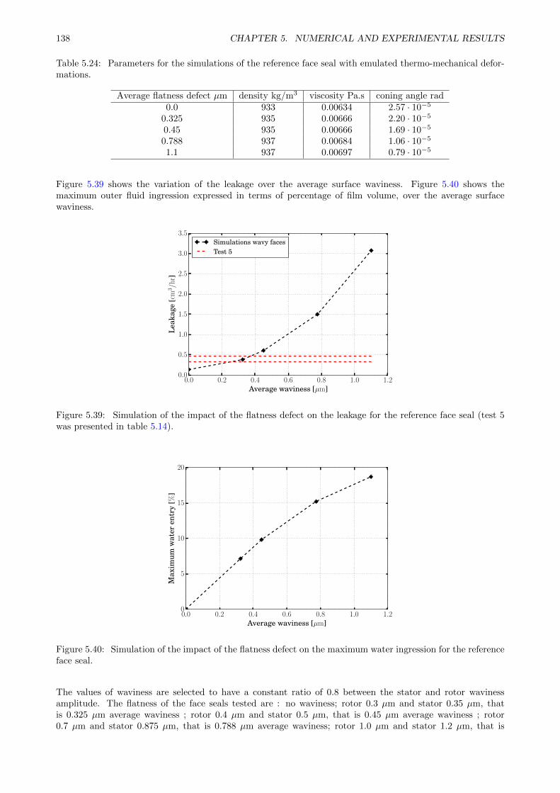
138 CHAPTER 5. NUMERICAL AND EXPERIMENTAL RESULTS
Table 5.24: Parameters for the simulations of the reference face seal with emulated thermo-mechanical defor-mations.
Average flatness defect µm density kg/m3 viscosity Pa.s coning angle rad0.0 933 0.00634 2.57 · 10−5
0.325 935 0.00666 2.20 · 10−5
0.45 935 0.00666 1.69 · 10−5
0.788 937 0.00684 1.06 · 10−5
1.1 937 0.00697 0.79 · 10−5
Figure 5.39 shows the variation of the leakage over the average surface waviness. Figure 5.40 shows themaximum outer fluid ingression expressed in terms of percentage of film volume, over the average surfacewaviness.
0.0 0.2 0.4 0.6 0.8 1.0 1.2Average waviness [µm]
0.0
0.5
1.0
1.5
2.0
2.5
3.0
3.5
Lea
kage
[cm
3/h
r]
Simulations wavy facesTest 5
Figure 5.39: Simulation of the impact of the flatness defect on the leakage for the reference face seal (test 5was presented in table 5.14).
0.0 0.2 0.4 0.6 0.8 1.0 1.2Average waviness [µm]
0
5
10
15
20
Max
imum
wat
eren
try
[%]
Figure 5.40: Simulation of the impact of the flatness defect on the maximum water ingression for the referenceface seal.
The values of waviness are selected to have a constant ratio of 0.8 between the stator and rotor wavinessamplitude. The flatness of the face seals tested are : no waviness; rotor 0.3 µm and stator 0.35 µm, thatis 0.325 µm average waviness ; rotor 0.4 µm and stator 0.5 µm, that is 0.45 µm average waviness ; rotor0.7 µm and stator 0.875 µm, that is 0.788 µm average waviness; rotor 1.0 µm and stator 1.2 µm, that is
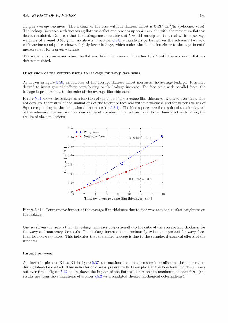
5.5. EFFECT OF WAVINESS 139
1.1 µm average waviness. The leakage of the case without flatness defect is 0.137 cm3/hr (reference case).The leakage increases with increasing flatness defect and reaches up to 3.1 cm3/hr with the maximum flatnessdefect simulated. One sees that the leakage measured for test 5 would correspond to a seal with an averagewaviness of around 0.325 µm. As shown in section 5.5.3, simulations performed on the reference face sealwith waviness and pulses show a slightly lower leakage, which makes the simulation closer to the experimentalmeasurement for a given waviness.
The water entry increases when the flatness defect increases and reaches 18.7% with the maximum flatnessdefect simulated.
Discussion of the contributions to leakage for wavy face seals
As shown in figure 5.39, an increase of the average flatness defect increases the average leakage. It is heredesired to investigate the effects contributing to the leakage increase. For face seals with parallel faces, theleakage is proportional to the cube of the average film thickness.
Figure 5.41 shows the leakage as a function of the cube of the average film thickness, averaged over time. Thered dots are the results of the simulations of the reference face seal without waviness and for various values ofSq (corresponding to the simulations done in section 5.2.1). The blue squares are the results of the simulationsof the reference face seal with various values of waviness. The red and blue dotted lines are trends fitting theresults of the simulations.
0 2 4 6 8 10 12 14 16
Time av. average cubic film thickness [µm3]
0.0
0.5
1.0
1.5
2.0
2.5
3.0
3.5
Lea
kage
[cm
3/h
r]
0.2016h3 + 0.15
0.1167h3 + 0.005
Wavy facesNon wavy faces
Figure 5.41: Comparative impact of the average film thickness due to face waviness and surface roughness onthe leakage.
One sees from the trends that the leakage increases proportionally to the cube of the average film thickness forthe wavy and non-wavy face seals. This leakage increase is approximately twice as important for wavy facesthan for non wavy faces. This indicates that the added leakage is due to the complex dynamical effects of thewaviness.
Impact on wear
As shown in pictures K1 to K4 in figure 5.37, the maximum contact pressure is localised at the inner radiusduring lobe-lobe contact. This indicates that wear preferentially takes place at the lobe level, which will wearout over time. Figure 5.42 below shows the impact of the flatness defect on the maximum contact force (theresults are from the simulations of section 5.5.2 with emulated thermo-mechanical deformations).
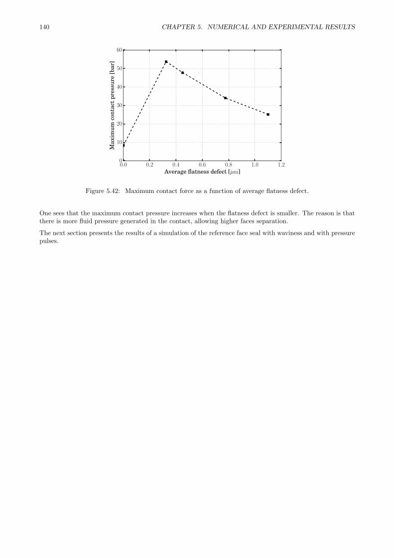
140 CHAPTER 5. NUMERICAL AND EXPERIMENTAL RESULTS
0.0 0.2 0.4 0.6 0.8 1.0 1.2Average flatness defect [µm]
0
10
20
30
40
50
60
Max
imum
cont
act
pres
sure
[bar
]
Figure 5.42: Maximum contact force as a function of average flatness defect.
One sees that the maximum contact pressure increases when the flatness defect is smaller. The reason is thatthere is more fluid pressure generated in the contact, allowing higher faces separation.
The next section presents the results of a simulation of the reference face seal with waviness and with pressurepulses.
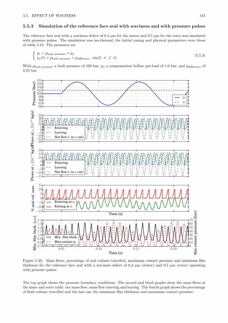
5.5. EFFECT OF WAVINESS 141
5.5.3 Simulation of the reference face seal with waviness and with pressure pulses
The reference face seal with a waviness defect of 0.4 µm for the stator and 0.5 µm for the rotor was simulatedwith pressure pulses. The simulation was iso-thermal, the initial coning and physical parameters were thoseof table 5.24. The pressures are
pi = pback pressure + pφpo(t) = pback pressure + pdifference · sin(2 · π · f · t) (5.5.3)
With pback pressure a back pressure of 100 bar, pφ a compensation bellow pre-load of 1.0 bar, and pdifference of3.55 bar.
96979899
100101102103104
Pre
ssur
e[b
ar]
po
pi
−20−15−10−5
05
10152025
Flo
ws
atr o
[10−
6kg
/s]
EnteringLeavingNet flow (- in + out)
−15−10−5
05
101520
Flo
ws
atr i
[10−
6kg
/s]
EnteringLeavingNet flow (- in + out)
Time [s]−15−10−5
05
1015
%se
alvo
l.tr
av.
Entering at roExiting at ri
0.05 0.10 0.15 0.20Time [s]
0.70.80.91.01.11.21.31.4
Min
.film
thic
k.[µ
m]
010203040506070
Max
cont
act
pres
sure
[bar
]
Min. film thick.Max contact p.
Figure 5.43: Mass flows, percentage of seal volume travelled, maximum contact pressure and minimum filmthickness for the reference face seal with a waviness defect of 0.4 µm (stator) and 0.5 µm (rotor) operatingwith pressure pulses
The top graph shows the pressure boundary conditions. The second and third graphs show the mass flows atthe inner and outer radii: net mass flow, mass flow entering and leaving. The fourth graph shows the percentageof fluid volume travelled and the last one the minimum film thickness and maximum contact pressure.
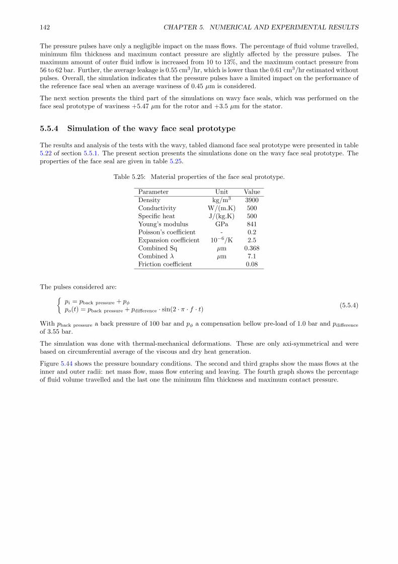
142 CHAPTER 5. NUMERICAL AND EXPERIMENTAL RESULTS
The pressure pulses have only a negligible impact on the mass flows. The percentage of fluid volume travelled,minimum film thickness and maximum contact pressure are slightly affected by the pressure pulses. Themaximum amount of outer fluid inflow is increased from 10 to 13%, and the maximum contact pressure from56 to 62 bar. Further, the average leakage is 0.55 cm3/hr, which is lower than the 0.61 cm3/hr estimated withoutpulses. Overall, the simulation indicates that the pressure pulses have a limited impact on the performance ofthe reference face seal when an average waviness of 0.45 µm is considered.
The next section presents the third part of the simulations on wavy face seals, which was performed on theface seal prototype of waviness +5.47 µm for the rotor and +3.5 µm for the stator.
5.5.4 Simulation of the wavy face seal prototype
The results and analysis of the tests with the wavy, tabled diamond face seal prototype were presented in table5.22 of section 5.5.1. The present section presents the simulations done on the wavy face seal prototype. Theproperties of the face seal are given in table 5.25.
Table 5.25: Material properties of the face seal prototype.
Parameter Unit ValueDensity kg/m3 3900Conductivity W/(m.K) 500Specific heat J/(kg.K) 500Young’s modulus GPa 841Poisson’s coefficient - 0.2Expansion coefficient 10−6/K 2.5Combined Sq µm 0.368Combined λ µm 7.1Friction coefficient 0.08
The pulses considered are:pi = pback pressure + pφpo(t) = pback pressure + pdifference · sin(2 · π · f · t) (5.5.4)
With pback pressure a back pressure of 100 bar and pφ a compensation bellow pre-load of 1.0 bar and pdifference
of 3.55 bar.
The simulation was done with thermal-mechanical deformations. These are only axi-symmetrical and werebased on circumferential average of the viscous and dry heat generation.
Figure 5.44 shows the pressure boundary conditions. The second and third graphs show the mass flows at theinner and outer radii: net mass flow, mass flow entering and leaving. The fourth graph shows the percentageof fluid volume travelled and the last one the minimum film thickness and maximum contact pressure.
5.5. EFFECT OF WAVINESS 143
96979899
100101102103104
Pre
ssur
e[b
ar]
po
pi
−400−300−200−100
0100200300400
Flo
ws
atr o
[10−
6kg
/s]
EnteringLeavingNet flow (- in + out)
−400−300−200−100
0100200300400
Flo
ws
atr i
[10−
6kg
/s]
EnteringLeavingNet flow (- in + out)
Time [s]−200−150−100−50
050
100
%se
alvo
l.tr
av.
Entering at roExiting at ri
0.05 0.10 0.15 0.20Time [s]
1.01.21.41.61.82.02.22.4
Min
.film
thic
k.[µ
m]
0255075100125150175
Max
cont
act
pres
sure
[bar
]
Min. film thick.Max contact p.
Figure 5.44: Mass flows, percentage of seal volume travelled, maximum contact pressure and minimum filmthickness for the diamond face seal of waviness 3.5 µm (stator) and 5.47 µm (rotor) operating with pressurepulses
The net flows vary between −350 · 10−6 kg/s to 350 · 10−6 kg/s, which is more than an order of magnitudeof the values of the reference face seal (see figure 5.36). The maximum outer radius inflow increases from288 · 10−6 kg/s to 372 · 10−6 kg/s due to the pulses. Similarly the maximum inner radius outflow changesfrom from 258 · 10−6 kg/s to 370 · 10−6 kg/s with the pulses. The change of outer fluid entry is also depictedby the fourth graph which indicates that, from the net mass flow, the outer fluid travels 150 % of the totalfilm volume. Based on this estimation, outer fluid ingression can be expected. Comparatively, the outer fluidtravels 26 % of the film volume when there are no pulses. These estimations are coherent with the experimentalresults, which indicate significant water entry, 1.1 %/hr, with pulses on that face seal; but limited withoutpulses 0.1 %/hr. The pressure pulses also increase the maximum contact pressure so that more wear can beexpected.
Further, the simulation indicates an average leakage of 109 cm3/hr at 80C. Similarly the same simulation at30C estimates an average leakage of 23 cm3/hr. These values are close to the experimental measurements,tests 9 and 11, as indicated in table 5.26 below.
144 CHAPTER 5. NUMERICAL AND EXPERIMENTAL RESULTS
Table 5.26: Average leakage for the wavy diamond face seal prototype.
Operating temperature Experiments Simulation30C 68± 10 cm3/hr 23 cm3/hr80C 78± 2− 126± 3 cm3/hr 109 cm3/hr
5.5.5 Conclusions from the study of the effect of face waviness
This section presented the results of an the experimental and numerical study of the impact of face waviness.A face seal with waviness of 5.47 µm for the rotor and 3.5 µm for the stator was tested on the setup. Themain experimental results are:
1. The pulses have a significant impact on the outer fluid ingression: an average increase of water of 1.0%to 1.1% per hour was measured with pulses, an average increase of water of 0.1% per hour was measuredwithout pulses.
2. The oil leakage is between 78 to 126 cm3 per hour when operating at 80C and 3500 rpm.
The simulation allowed to highlight a significant film squeeze and stretching effect due to the rotation of thewavy surfaces. Such effects lead to inflows and outflows at both radii. The following analysis can be made:
The surface waviness, which always exists to some extent, increases the leakage significantly. For thereference face seal, the leakage increases from 0.137 cm3/hr with no waviness to 3.1 cm3/hr with arotor waviness of 1.0 µm and stator waviness of 1.2 µm. The volume loss measured for test 5 of 144 hcorrespond to the value predicted for a face seal of waviness of 0.325 µm which is close to the measuredwaviness.
Based on instantaneous circumferential average mass flows, the wavy face seal prototype is expected toshow water ingression under pulses. This observation is in line with the experimental measurements.
The simulation indicates a leakage of 109 cm3/hr at 80C and of 23 cm3/hr at 30C for the face sealprototype, which is close to the measured values of 78± 2− 126± 3 cm3/hr at 80C and 68± 10 cm3/hrat 30C.
The addition of a transport equation for the outer fluid should be considered as this would allow betterestimating the outer fluid ingression and making quantitative comparisons.
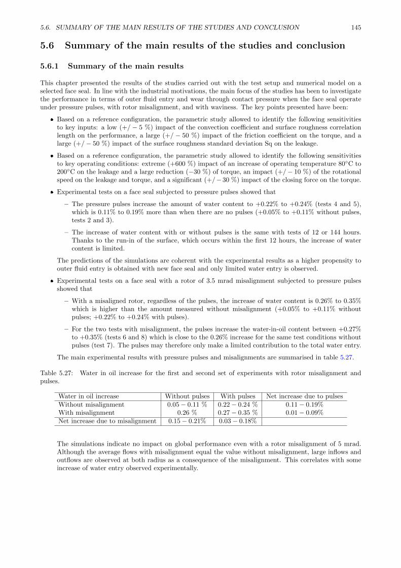
5.6. SUMMARY OF THE MAIN RESULTS OF THE STUDIES AND CONCLUSION 145
5.6 Summary of the main results of the studies and conclusion
5.6.1 Summary of the main results
This chapter presented the results of the studies carried out with the test setup and numerical model on aselected face seal. In line with the industrial motivations, the main focus of the studies has been to investigatethe performance in terms of outer fluid entry and wear through contact pressure when the face seal operateunder pressure pulses, with rotor misalignment, and with waviness. The key points presented have been:
Based on a reference configuration, the parametric study allowed to identify the following sensitivitiesto key inputs: a low (+/ − 5 %) impact of the convection coefficient and surface roughness correlationlength on the performance, a large (+/ − 50 %) impact of the friction coefficient on the torque, and alarge (+/− 50 %) impact of the surface roughness standard deviation Sq on the leakage.
Based on a reference configuration, the parametric study allowed to identify the following sensitivitiesto key operating conditions: extreme (+600 %) impact of an increase of operating temperature 80C to200C on the leakage and a large reduction (−30 %) of torque, an impact (+/− 10 %) of the rotationalspeed on the leakage and torque, and a significant (+/−30 %) impact of the closing force on the torque.
Experimental tests on a face seal subjected to pressure pulses showed that
– The pressure pulses increase the amount of water content to +0.22% to +0.24% (tests 4 and 5),which is 0.11% to 0.19% more than when there are no pulses (+0.05% to +0.11% without pulses,tests 2 and 3).
– The increase of water content with or without pulses is the same with tests of 12 or 144 hours.Thanks to the run-in of the surface, which occurs within the first 12 hours, the increase of watercontent is limited.
The predictions of the simulations are coherent with the experimental results as a higher propensity toouter fluid entry is obtained with new face seal and only limited water entry is observed.
Experimental tests on a face seal with a rotor of 3.5 mrad misalignment subjected to pressure pulsesshowed that
– With a misaligned rotor, regardless of the pulses, the increase of water content is 0.26% to 0.35%which is higher than the amount measured without misalignment (+0.05% to +0.11% withoutpulses; +0.22% to +0.24% with pulses).
– For the two tests with misalignment, the pulses increase the water-in-oil content between +0.27%to +0.35% (tests 6 and 8) which is close to the 0.26% increase for the same test conditions withoutpulses (test 7). The pulses may therefore only make a limited contribution to the total water entry.
The main experimental results with pressure pulses and misalignments are summarised in table 5.27.
Table 5.27: Water in oil increase for the first and second set of experiments with rotor misalignment andpulses.
Water in oil increase Without pulses With pulses Net increase due to pulsesWithout misalignment 0.05− 0.11 % 0.22− 0.24 % 0.11− 0.19%With misalignment 0.26 % 0.27− 0.35 % 0.01− 0.09%Net increase due to misalignment 0.15− 0.21% 0.03− 0.18%
The simulations indicate no impact on global performance even with a rotor misalignment of 5 mrad.Although the average flows with misalignment equal the value without misalignment, large inflows andoutflows are observed at both radius as a consequence of the misalignment. This correlates with someincrease of water entry observed experimentally.
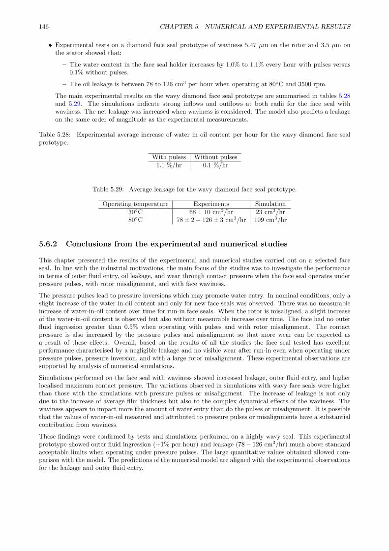
146 CHAPTER 5. NUMERICAL AND EXPERIMENTAL RESULTS
Experimental tests on a diamond face seal prototype of waviness 5.47 µm on the rotor and 3.5 µm onthe stator showed that:
– The water content in the face seal holder increases by 1.0% to 1.1% every hour with pulses versus0.1% without pulses.
– The oil leakage is between 78 to 126 cm3 per hour when operating at 80C and 3500 rpm.
The main experimental results on the wavy diamond face seal prototype are summarised in tables 5.28and 5.29. The simulations indicate strong inflows and outflows at both radii for the face seal withwaviness. The net leakage was increased when waviness is considered. The model also predicts a leakageon the same order of magnitude as the experimental measurements.
Table 5.28: Experimental average increase of water in oil content per hour for the wavy diamond face sealprototype.
With pulses Without pulses1.1 %/hr 0.1 %/hr
Table 5.29: Average leakage for the wavy diamond face seal prototype.
Operating temperature Experiments Simulation30C 68± 10 cm3/hr 23 cm3/hr80C 78± 2− 126± 3 cm3/hr 109 cm3/hr
5.6.2 Conclusions from the experimental and numerical studies
This chapter presented the results of the experimental and numerical studies carried out on a selected faceseal. In line with the industrial motivations, the main focus of the studies was to investigate the performancein terms of outer fluid entry, oil leakage, and wear through contact pressure when the face seal operates underpressure pulses, with rotor misalignment, and with face waviness.
The pressure pulses lead to pressure inversions which may promote water entry. In nominal conditions, only aslight increase of the water-in-oil content and only for new face seals was observed. There was no measurableincrease of water-in-oil content over time for run-in face seals. When the rotor is misaligned, a slight increaseof the water-in-oil content is observed but also without measurable increase over time. The face had no outerfluid ingression greater than 0.5% when operating with pulses and with rotor misalignment. The contactpressure is also increased by the pressure pulses and misalignment so that more wear can be expected asa result of these effects. Overall, based on the results of all the studies the face seal tested has excellentperformance characterised by a negligible leakage and no visible wear after run-in even when operating underpressure pulses, pressure inversion, and with a large rotor misalignment. These experimental observations aresupported by analysis of numerical simulations.
Simulations performed on the face seal with waviness showed increased leakage, outer fluid entry, and higherlocalised maximum contact pressure. The variations observed in simulations with wavy face seals were higherthan those with the simulations with pressure pulses or misalignment. The increase of leakage is not onlydue to the increase of average film thickness but also to the complex dynamical effects of the waviness. Thewaviness appears to impact more the amount of water entry than do the pulses or misalignment. It is possiblethat the values of water-in-oil measured and attributed to pressure pulses or misalignments have a substantialcontribution from waviness.
These findings were confirmed by tests and simulations performed on a highly wavy seal. This experimentalprototype showed outer fluid ingression (+1% per hour) and leakage (78− 126 cm3/hr) much above standardacceptable limits when operating under pressure pulses. The large quantitative values obtained allowed com-parison with the model. The predictions of the numerical model are aligned with the experimental observationsfor the leakage and outer fluid entry.
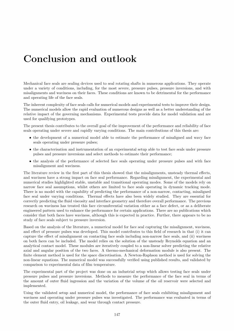
Conclusion and outlook
Mechanical face seals are sealing devices used to seal rotating shafts in numerous applications. They operateunder a variety of conditions, including, for the most severe, pressure pulses, pressure inversions, and withmisalignments and waviness on their faces. These conditions are known to be detrimental for the performanceand operating life of the face seals.
The inherent complexity of face seals calls for numerical models and experimental tests to improve their design.The numerical models allow the rapid evaluation of numerous designs as well as a better understanding of therelative impact of the governing mechanisms. Experimental tests provide data for model validation and areused for qualifying prototypes.
The present thesis contributes to the overall goal of the improvement of the performance and reliability of faceseals operating under severe and rapidly varying conditions. The main contributions of this thesis are:
the development of a numerical model able to estimate the performance of misaligned and wavy faceseals operating under pressure pulses;
the characterisation and instrumentation of an experimental setup able to test face seals under pressurepulses and pressure inversions and select methods to estimate their performance;
the analysis of the performance of selected face seals operating under pressure pulses and with facemisalignment and waviness.
The literature review in the first part of this thesis showed that the misalignments, unsteady thermal effects,and waviness have a strong impact on face seal performance. Regarding misalignment, the experimental andnumerical studies highlighted stable, unstable and transitional operating modes. Some of the models rely onnarrow face seal assumptions, whilst others are limited to face seals operating in dynamic tracking mode.There is no model with the capability of predicting the performance of a non-narrow, contacting, misalignedface seal under varying conditions. Thermal effects have also been widely studied. They are essential forcorrectly predicting the fluid viscosity and interface geometry and therefore overall performance. The previousresearch on waviness has treated this face circumferential variation either as a face defect, or as a deliberateengineered pattern used to enhance the performance for certain applications. There are no publications whichconsider that both faces have waviness, although this is expected in practice. Further, there appears to be nostudy of face seals subject to pressure inversion.
Based on the analysis of the literature, a numerical model for face seal capturing the misalignment, waviness,and effect of pressure pulses was developed. This model contributes to this field of research in that (i) it cancapture the effect of misalignment on contacting face seals including non-narrow face seals, and (ii) wavinesson both faces can be included. The model relies on the solution of the unsteady Reynolds equation and ananalytical contact model. These modules are iteratively coupled to a non-linear solver predicting the relativeaxial and angular position of the two faces. A thermo-mechanical deformation module is also present. Thefinite element method is used for the space discretisation. A Newton-Raphson method is used for solving thenon-linear equations. The numerical model was successfully verified using published results, and validated bycomparison to experimental data of film temperature.
The experimental part of the project was done on an industrial setup which allows testing face seals underpressure pulses and pressure inversions. Methods to measure the performance of the face seal in terms ofthe amount of outer fluid ingression and the variation of the volume of the oil reservoir were selected andimplemented.
Using the validated setup and numerical model, the performance of face seals exhibiting misalignment andwaviness and operating under pressure pulses was investigated. The performance was evaluated in terms ofthe outer fluid entry, oil leakage, and wear through contact pressure.
147
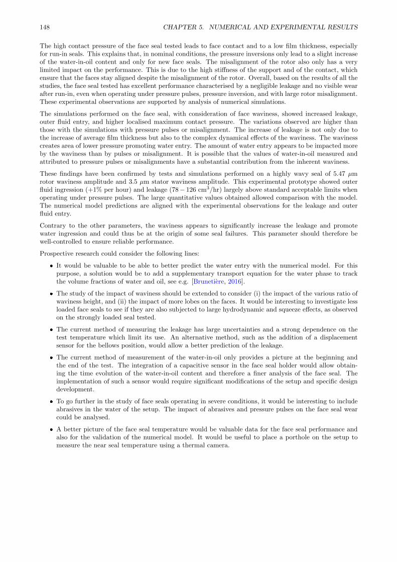
148 CHAPTER 5. NUMERICAL AND EXPERIMENTAL RESULTS
The high contact pressure of the face seal tested leads to face contact and to a low film thickness, especiallyfor run-in seals. This explains that, in nominal conditions, the pressure inversions only lead to a slight increaseof the water-in-oil content and only for new face seals. The misalignment of the rotor also only has a verylimited impact on the performance. This is due to the high stiffness of the support and of the contact, whichensure that the faces stay aligned despite the misalignment of the rotor. Overall, based on the results of all thestudies, the face seal tested has excellent performance characterised by a negligible leakage and no visible wearafter run-in, even when operating under pressure pulses, pressure inversion, and with large rotor misalignment.These experimental observations are supported by analysis of numerical simulations.
The simulations performed on the face seal, with consideration of face waviness, showed increased leakage,outer fluid entry, and higher localised maximum contact pressure. The variations observed are higher thanthose with the simulations with pressure pulses or misalignment. The increase of leakage is not only due tothe increase of average film thickness but also to the complex dynamical effects of the waviness. The wavinesscreates area of lower pressure promoting water entry. The amount of water entry appears to be impacted moreby the waviness than by pulses or misalignment. It is possible that the values of water-in-oil measured andattributed to pressure pulses or misalignments have a substantial contribution from the inherent waviness.
These findings have been confirmed by tests and simulations performed on a highly wavy seal of 5.47 µmrotor waviness amplitude and 3.5 µm stator waviness amplitude. This experimental prototype showed outerfluid ingression (+1% per hour) and leakage (78− 126 cm3/hr) largely above standard acceptable limits whenoperating under pressure pulses. The large quantitative values obtained allowed comparison with the model.The numerical model predictions are aligned with the experimental observations for the leakage and outerfluid entry.
Contrary to the other parameters, the waviness appears to significantly increase the leakage and promotewater ingression and could thus be at the origin of some seal failures. This parameter should therefore bewell-controlled to ensure reliable performance.
Prospective research could consider the following lines:
It would be valuable to be able to better predict the water entry with the numerical model. For thispurpose, a solution would be to add a supplementary transport equation for the water phase to trackthe volume fractions of water and oil, see e.g. [Brunetiere, 2016].
The study of the impact of waviness should be extended to consider (i) the impact of the various ratio ofwaviness height, and (ii) the impact of more lobes on the faces. It would be interesting to investigate lessloaded face seals to see if they are also subjected to large hydrodynamic and squeeze effects, as observedon the strongly loaded seal tested.
The current method of measuring the leakage has large uncertainties and a strong dependence on thetest temperature which limit its use. An alternative method, such as the addition of a displacementsensor for the bellows position, would allow a better prediction of the leakage.
The current method of measurement of the water-in-oil only provides a picture at the beginning andthe end of the test. The integration of a capacitive sensor in the face seal holder would allow obtain-ing the time evolution of the water-in-oil content and therefore a finer analysis of the face seal. Theimplementation of such a sensor would require significant modifications of the setup and specific designdevelopment.
To go further in the study of face seals operating in severe conditions, it would be interesting to includeabrasives in the water of the setup. The impact of abrasives and pressure pulses on the face seal wearcould be analysed.
A better picture of the face seal temperature would be valuable data for the face seal performance andalso for the validation of the numerical model. It would be useful to place a porthole on the setup tomeasure the near seal temperature using a thermal camera.
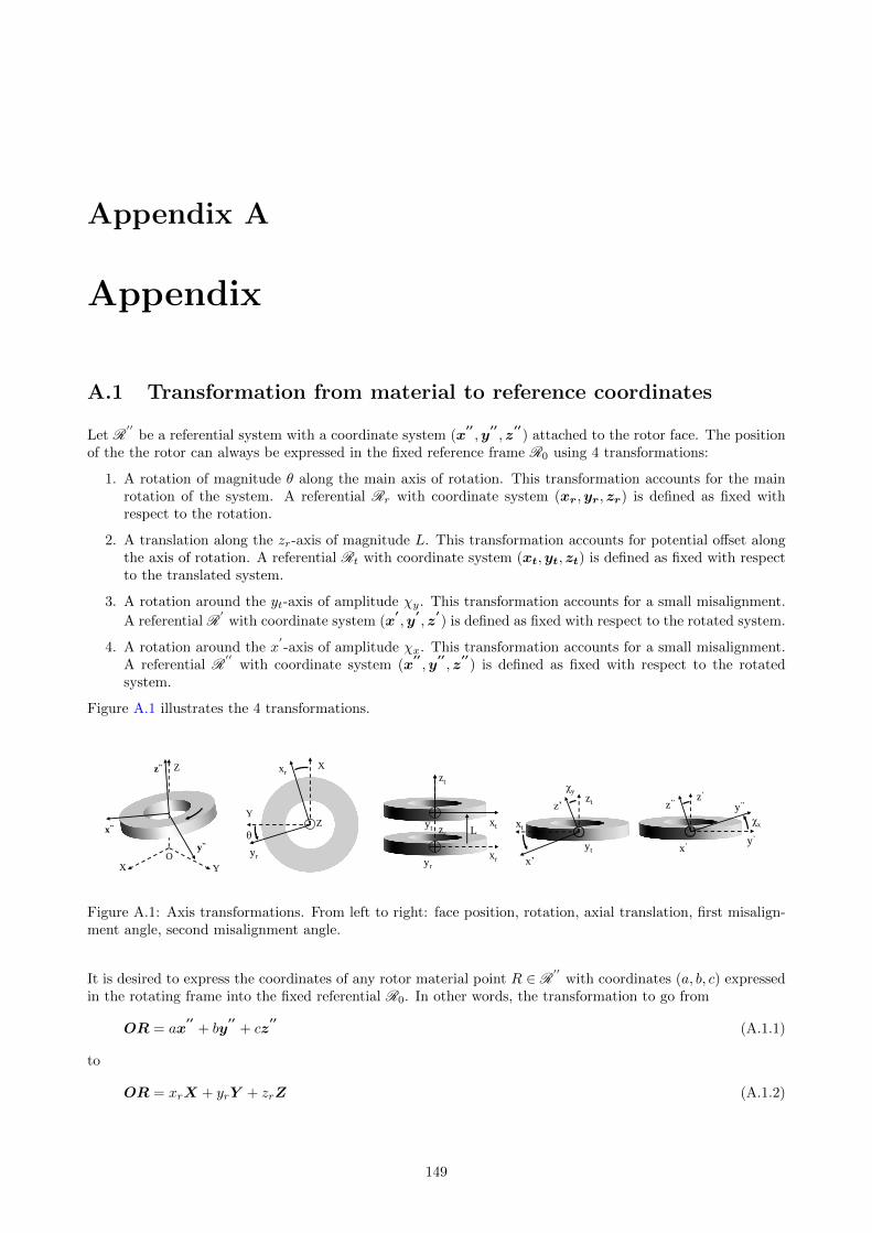
Appendix A
Appendix
A.1 Transformation from material to reference coordinates
Let R′′
be a referential system with a coordinate system (x′′,y
′′, z
′′) attached to the rotor face. The position
of the the rotor can always be expressed in the fixed reference frame R0 using 4 transformations:
1. A rotation of magnitude θ along the main axis of rotation. This transformation accounts for the mainrotation of the system. A referential Rr with coordinate system (xr,yr, zr) is defined as fixed withrespect to the rotation.
2. A translation along the zr-axis of magnitude L. This transformation accounts for potential offset alongthe axis of rotation. A referential Rt with coordinate system (xt,yt, zt) is defined as fixed with respectto the translated system.
3. A rotation around the yt-axis of amplitude χy. This transformation accounts for a small misalignment.
A referential R′
with coordinate system (x′,y
′, z
′) is defined as fixed with respect to the rotated system.
4. A rotation around the x′-axis of amplitude χx. This transformation accounts for a small misalignment.
A referential R′′
with coordinate system (x′′,y
′′, z
′′) is defined as fixed with respect to the rotated
system.
Figure A.1 illustrates the 4 transformations.
xr
xt
yr
yt zr
zt
L
YX
Zz’’
x’’
y’’
O
zt
yt
xt
z’
x’
χy
X
Y
xr
yr
Z
θy’
z’
χx
z’’ y’’
x’
Figure A.1: Axis transformations. From left to right: face position, rotation, axial translation, first misalign-ment angle, second misalignment angle.
It is desired to express the coordinates of any rotor material point R ∈ R′′
with coordinates (a, b, c) expressedin the rotating frame into the fixed referential R0. In other words, the transformation to go from
OR = ax′′
+ by′′
+ cz′′
(A.1.1)
to
OR = xrX + yrY + zrZ (A.1.2)
149
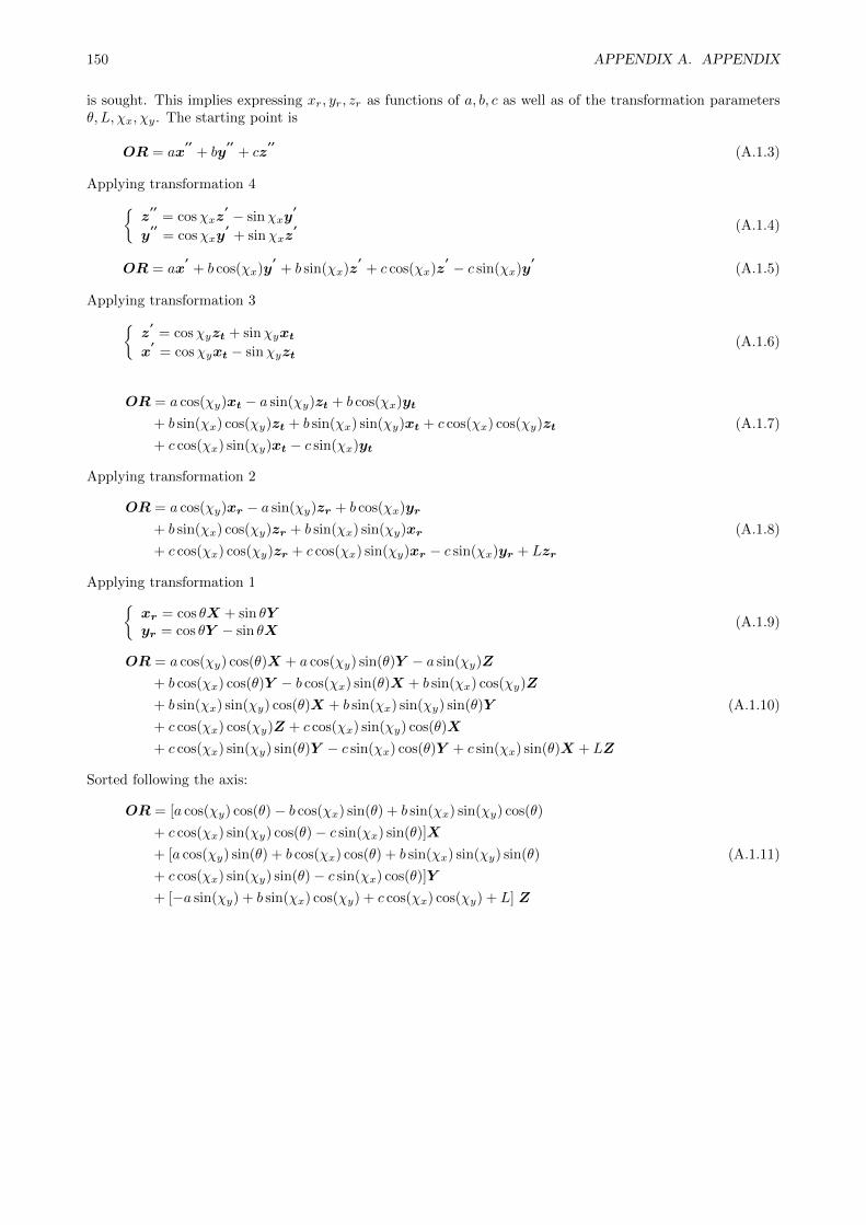
150 APPENDIX A. APPENDIX
is sought. This implies expressing xr, yr, zr as functions of a, b, c as well as of the transformation parametersθ, L, χx, χy. The starting point is
OR = ax′′
+ by′′
+ cz′′
(A.1.3)
Applying transformation 4z
′′= cosχxz
′ − sinχxy′
y′′
= cosχxy′
+ sinχxz′ (A.1.4)
OR = ax′
+ b cos(χx)y′
+ b sin(χx)z′
+ c cos(χx)z′ − c sin(χx)y
′(A.1.5)
Applying transformation 3z
′= cosχyzt + sinχyxt
x′
= cosχyxt − sinχyzt(A.1.6)
OR = a cos(χy)xt − a sin(χy)zt + b cos(χx)yt
+ b sin(χx) cos(χy)zt + b sin(χx) sin(χy)xt + c cos(χx) cos(χy)zt
+ c cos(χx) sin(χy)xt − c sin(χx)yt
(A.1.7)
Applying transformation 2
OR = a cos(χy)xr − a sin(χy)zr + b cos(χx)yr
+ b sin(χx) cos(χy)zr + b sin(χx) sin(χy)xr
+ c cos(χx) cos(χy)zr + c cos(χx) sin(χy)xr − c sin(χx)yr + Lzr
(A.1.8)
Applying transformation 1xr = cos θX + sin θYyr = cos θY − sin θX
(A.1.9)
OR = a cos(χy) cos(θ)X + a cos(χy) sin(θ)Y − a sin(χy)Z
+ b cos(χx) cos(θ)Y − b cos(χx) sin(θ)X + b sin(χx) cos(χy)Z
+ b sin(χx) sin(χy) cos(θ)X + b sin(χx) sin(χy) sin(θ)Y
+ c cos(χx) cos(χy)Z + c cos(χx) sin(χy) cos(θ)X
+ c cos(χx) sin(χy) sin(θ)Y − c sin(χx) cos(θ)Y + c sin(χx) sin(θ)X + LZ
(A.1.10)
Sorted following the axis:
OR = [a cos(χy) cos(θ)− b cos(χx) sin(θ) + b sin(χx) sin(χy) cos(θ)
+ c cos(χx) sin(χy) cos(θ)− c sin(χx) sin(θ)]X
+ [a cos(χy) sin(θ) + b cos(χx) cos(θ) + b sin(χx) sin(χy) sin(θ)
+ c cos(χx) sin(χy) sin(θ)− c sin(χx) cos(θ)]Y
+ [−a sin(χy) + b sin(χx) cos(χy) + c cos(χx) cos(χy) + L] Z
(A.1.11)
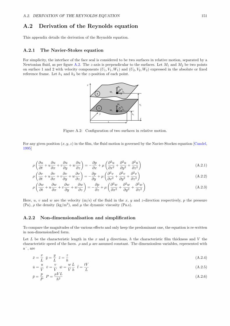
A.2. DERIVATION OF THE REYNOLDS EQUATION 151
A.2 Derivation of the Reynolds equation
This appendix details the derivation of the Reynolds equation.
A.2.1 The Navier-Stokes equation
For simplicity, the interface of the face seal is considered to be two surfaces in relative motion, separated by aNewtonian fluid, as per figure A.2. The z-axis is perpendicular to the surfaces. Let M1 and M2 be two pointson surface 1 and 2 with velocity components (U1, V1,W1) and (U2, V2,W2) expressed in the absolute or fixedreference frame. Let h1 and h2 be the z-position of each point.
𝑦
𝑥
𝑧
M2
M1
h1
h2
W2
U2
V2
W1
V1
U1
L
1
2
Figure A.2: Configuration of two surfaces in relative motion.
For any given position (x, y, z) in the film, the fluid motion is governed by the Navier-Stockes equation [Candel,1995]
ρ
(∂u
∂t+ u
∂u
∂x+ v
∂u
∂y+ w
∂u
∂z
)= −∂p
∂x+ µ
(∂2u
∂x2+∂2u
∂y2+∂2u
∂z2
)(A.2.1)
ρ
(∂v
∂t+ u
∂v
∂x+ v
∂v
∂y+ w
∂v
∂z
)= −∂p
∂y+ µ
(∂2v
∂x2+∂2v
∂y2+∂2v
∂z2
)(A.2.2)
ρ
(∂w
∂t+ u
∂w
∂x+ v
∂w
∂y+ w
∂w
∂z
)= −∂p
∂z+ µ
(∂2w
∂x2+∂2w
∂y2+∂2w
∂z2
)(A.2.3)
Here, u, v and w are the velocity (m/s) of the fluid in the x, y and z-direction respectively, p the pressure(Pa), ρ the density (kg/m3), and µ the dynamic viscosity (Pa.s).
A.2.2 Non-dimensionalisation and simplification
To compare the magnitudes of the various effects and only keep the predominant one, the equation is re-writtenin non-dimensionlised form.
Let L be the characteristic length in the x and y directions, h the characteristic film thickness and V thecharacteristic speed of the faces. ρ and µ are assumed constant. The dimensionless variables, represented witha¯, are
x =x
Ly =
y
Lz =
z
h(A.2.4)
u =u
Vv =
v
Vw =
w
V
L
ht =
tV
L(A.2.5)
p =p
PP =
µV L
h2(A.2.6)
152 APPENDIX A. APPENDIX
Substituting yields
Re ε
(∂u
∂t+ u
∂u
∂x+ v
∂u
∂y+ w
∂u
∂z
)= −∂p
∂x+
(ε2∂2u
∂x2+ ε2
∂2u
∂y2+∂2u
∂z2
)(A.2.7)
Re ε
(∂v
∂t+ u
∂v
∂x+ v
∂v
∂y+ w
∂v
∂z
)= −∂p
∂y+
(ε2∂2v
∂x2+ ε2
∂2v
∂y2+∂2v
∂z2
)(A.2.8)
Re ε3(∂w
∂t+ u
∂w
∂x+ v
∂w
∂y+ w
∂w
∂z
)= −∂p
∂z+
(ε4∂2w
∂x2+ ε4
∂2w
∂y2+ ε2
∂2w
∂z2
)(A.2.9)
with
ε =h
LRe =
ρV h
µ(A.2.10)
which controls the order of the terms in the equation. For liquid face seals, such as those of interest here, onetypically has: h ∼ 10−6 m, L ∼ 10−2 m, ρ ∼ 103 kg/m3, V ∼ 1 − 10 m/s, µ ∼ 10−3 Pa.s; thus ε < 10−3,Re < 10.
By keeping only first order terms (and re-using dimensional variables), the equations become
∂p
∂x=
∂
∂z
(µ∂u
∂z
)(A.2.11)
∂p
∂y=
∂
∂z
(µ∂v
∂z
)(A.2.12)
∂p
∂z= 0 (A.2.13)
The last equation indicates that the pressure is supposed constant along the film thickness. The two firstequations are integrated to express the velocity as a function of the pressure gradient.
Remark: For a high-speed, large, liquid face seal, the magnitude of the parameters are different and sup-plementary centrifugal inertia terms should be included, see e.g. [Rouillon, 2017] or [Brunetiere, 2016].
A.2.3 Velocity profiles
For simplicity, without losing generality, one sets h = h2 − h1 and h1 = 0. Assuming constant pressure alongthe thickness, the integration of equation A.2.11 gives∫ h
0
∂
∂z
(µ∂u
∂z
)dz =
∫ h
0
∂p
∂xdz ⇒ u(z) =
1
2µ
∂p
∂xz2 + C1z + C2 (A.2.14)
with C1 and C2 two integration constants determined by the boundary conditions. One assumes that the fluidadheres to the walls (i.e. the speed of the fluid at a wall equals the wall speed): u(z = h1 = 0) = U1 andu(z = h2) = U2. Using these boundary conditions, the velocity becomes
u(z) =1
2µ
∂p
∂xz2 + z
(U2 − U1
h− 1
2µ
∂p
∂xh
)+ U1 (A.2.15)
in a similar fashion for v
v(z) =1
2µ
∂p
∂yz2 + z
(V2 − V1
h− 1
2µ
∂p
∂yh
)+ V1 (A.2.16)
The velocity equations are left in this form to ease the further integration. The form below is sometimespreferred to underline the contributions of the velocity profile
v(z) =1
2µ
∂p
∂y(z2 − zh) + z
V2 − V1
h+ V1 (A.2.17)
One sees that the velocity is the sum of two contributions:
A Poiseuille flow due to a pressure gradient ∂p/∂y. This effect leads to parabolic shape of the velocityprofile(z2 dependency)
A Couette flow due to wall velocities V1 and V2. This effects leads to a linear shape of the velocity profile(z dependency)
A.2. DERIVATION OF THE REYNOLDS EQUATION 153
A.2.4 Mass conservation
To proceed with the derivation, the mass conservation equation is integrated over the film thickness∫ h
0
(∂ρ
∂t+∂ρu
∂x+∂ρv
∂y+∂ρw
∂z
)dz = 0 (A.2.18)
The next step is to use the Leibniz integration rule to take the space derivative out of the integral (see e.g. the’general integration rule’ of [Hamrock et al., 2004])1. Applied to the terms separately for clarity, one obtains∫ h
0
∂ρu
∂xdz = −(ρu)h
∂h
∂x
∣∣∣∣h
+ (ρu)h=0∂h
∂x
∣∣∣∣h=0
+∂
∂x
∫ h
0
ρudz (A.2.19)
= −ρU2∂h2
∂x+ ρU1
∂h1
∂x+
∂
∂x
∫ h
0
ρudz (A.2.20)
Considering a constant density over the film thickness, it is taken out of the integral in equation A.2.20. Usingequation A.2.15, the remaining integral of velocity is∫ h
0
udz =
∫ h
0
1
2µ
∂p
∂xz2dz +
∫ h
0
z
(U2 − U1
h− 1
2µ
∂p
∂xh
)dz +
∫ h
0
U1dz (A.2.21)
=1
6µ
∂p
∂xh3 +
(U2 − U1)h
2− 1
4µ
∂p
∂xh3 + U1h (A.2.22)
= − 1
12µ
∂p
∂xh3 +
(U2 + U1)h
2(A.2.23)
In the same manner∫ h
0
∂ρv
∂ydz = −ρV2
∂h2
∂y+ ρV1
∂h1
∂y+
∂
∂y
∫ h
0
ρvdz (A.2.24)
with, from integration equation A.2.16 gives∫ h
0
vdz = − 1
12µ
∂p
∂yh3 +
(V2 + V1)h
2(A.2.25)
Besides∫ h
0
∂ρw
∂zdz = ρ(w2 − w1) (A.2.26)
Substituting equations A.2.20, A.2.23, A.2.24, A.2.25, A.2.26 into A.2.18 gives
0 = h∂ρ
∂t− ρU2
∂h2
∂x+ ρU1
∂h1
∂x− ∂
∂x
ρ
12µ
∂p
∂xh3 +
∂
∂xρ
(U2 + U1)h
2
− ρV2∂h2
∂x+ ρV1
∂h1
∂x− ∂
∂y
ρ
12µ
∂p
∂yh3 +
∂
∂yρ
(V2 + V1)h
2
+ ρ(W2 −W1)
(A.2.27)
One recognises (see the proof in the subsequent section A.2.5)
∂h
∂t= W2 − U2
∂h2
∂x− V2
∂h2
∂y−W1 + U1
∂h1
∂x+ V1
∂h1
∂y(A.2.28)
And employing the chain rule on ρh
ρ∂h
∂t+ h
∂ρ
∂t=
∂
∂t(ρh) (A.2.29)
A compact form of the Reynolds equation is obtained
∂
∂x
(ρh3
µ
∂p
∂x
)+
∂
∂y
(ρh3
µ
∂p
∂y
)= 6
∂
∂x[(U1 + U2) ρh] + 6
∂
∂y[(V1 + V2) ρh] + 12
∂
∂t(ρh) (A.2.30)
For the case of interest, the velocities of face number 2, i.e., the stator, are zero: U2 = V2 = 0. The velocities ofthe rotor are U1 = −yω and V1 = xω (see section A.2.6). With these consideration the form shown in section2.2.3 is obtained.
1see also Leibniz integration rule, [Szeri, 2011]
154 APPENDIX A. APPENDIX
A.2.5 Partial derivative of the film thickness with respect to time
For face (1), one has
dh1 =∂h1
∂XdX1 +
∂h1
∂YdY1 +
∂h1
∂tdt (A.2.31)
∂h1
∂t=
dh1
dt− ∂h1
∂X
dX1
dt− ∂h1
∂Y
dY1
dt(A.2.32)
∂h1
∂t= W1 −
∂h1
∂XU1 −
∂h1
∂YV1 (A.2.33)
Similarly, for face (2)
∂h2
∂t= W2 −
∂h2
∂XU2 −
∂h2
∂YV2 (A.2.34)
By combining subtracting the face heights with face (2) above as per convection, one obtains the film thickness
∂h
∂t=∂h2
∂t− ∂h1
∂t(A.2.35)
∂h
∂t= −W1 +W2 +
∂h1
∂XU1 −
∂h2
∂XU2 +
∂h1
∂YV1 −
∂h2
∂YV2 (A.2.36)
A.2.6 Face velocities
The velocities of the faces U and V used in the derivation of the Reynolds equation are obtained by differen-tiating the corresponding component of the vector OR or OS with respect to time
U1 =dx
dt=
dx
dθ
dθ
dt= (−a sin(θ)− b cos(θ))θ = −yθ = −yω (A.2.37)
V1 =dy
dt=
dy
dθ
dθ
dt= (a cos(θ)− b sin(θ))θ = xθ = xω (A.2.38)
U2 = −(d sin(θ2) + e cos(θ2))θ2 = −yθ2 = 0 (A.2.39)
V2 = (d cos(θ2)− e sin(θ2))θ2 = xθ2 = 0 (A.2.40)
with ω the rotor’s rotational speed. The velocity of the stator’s faces is zero because in practice the linkageelements prevent the stator from rotating, that is, θ2 = 0, thus U2 = V2 = 0.
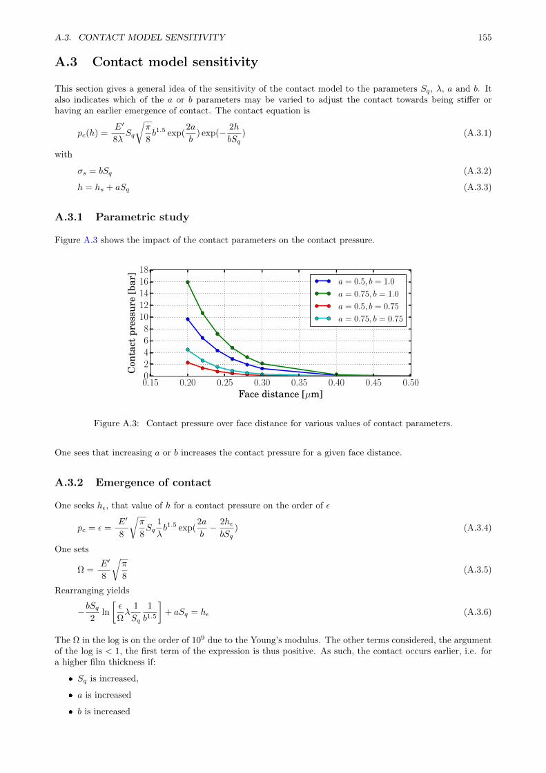
A.3. CONTACT MODEL SENSITIVITY 155
A.3 Contact model sensitivity
This section gives a general idea of the sensitivity of the contact model to the parameters Sq, λ, a and b. Italso indicates which of the a or b parameters may be varied to adjust the contact towards being stiffer orhaving an earlier emergence of contact. The contact equation is
pc(h) =E′
8λSq
√π
8b1.5 exp(
2a
b) exp(− 2h
bSq) (A.3.1)
with
σs = bSq (A.3.2)
h = hs + aSq (A.3.3)
A.3.1 Parametric study
Figure A.3 shows the impact of the contact parameters on the contact pressure.
0.15 0.20 0.25 0.30 0.35 0.40 0.45 0.50Face distance [µm]
02468
1012141618
Con
tact
pres
sure
[bar
]
a = 0.5, b = 1.0
a = 0.75, b = 1.0
a = 0.5, b = 0.75
a = 0.75, b = 0.75
Figure A.3: Contact pressure over face distance for various values of contact parameters.
One sees that increasing a or b increases the contact pressure for a given face distance.
A.3.2 Emergence of contact
One seeks hε, that value of h for a contact pressure on the order of ε
pc = ε =E′
8
√π
8Sq
1
λb1.5 exp(
2a
b− 2hεbSq
) (A.3.4)
One sets
Ω =E′
8
√π
8(A.3.5)
Rearranging yields
−bSq2
ln
[ε
Ωλ
1
Sq
1
b1.5
]+ aSq = hε (A.3.6)
The Ω in the log is on the order of 109 due to the Young’s modulus. The other terms considered, the argumentof the log is < 1, the first term of the expression is thus positive. As such, the contact occurs earlier, i.e. fora higher film thickness if:
Sq is increased,
a is increased
b is increased
156 APPENDIX A. APPENDIX
A.3.3 Contact model stiffness sensitivity
Differentiating equation A.3.4 with respect to h yields
∂pc∂h
= ΩSqλb1.5−2
bSqexp(
2a
b− 2h
bSq) (A.3.7)
or
∂pc∂h
= −2Ω1
λ
√b exp(
2
b
(a− h
Sq
)) (A.3.8)
h is on the order of 2 to 4 times Sq, while a and b are on the order of unity. Therefore, the contact is stiffer if
b is increased
a is increased
Sq is increased
λ is decreased
Ω, that is, E′ is increased.
The argument in the exponential is close to 0, hence the exponential can be developed as a series to the firstterm 1.
A.3.4 Conclusion
For a surface of given Sq and λ, the contact model:
can be set stiffer by increasing b
can be set to have an emerging contact for higher thickness, by increasing a (preferentially) or b
For two surface of different Sq and λ, the contact model is stiffer and has an earlier emergence of contact forthe surface with the higher Sq and λ.
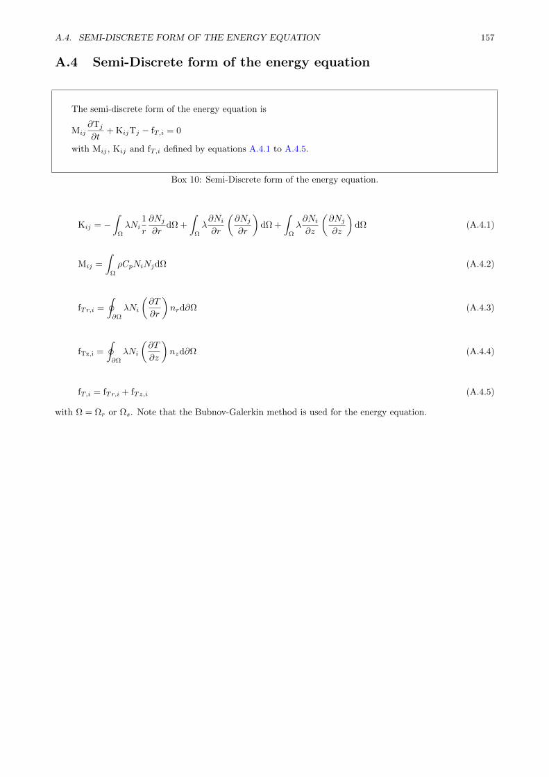
A.4. SEMI-DISCRETE FORM OF THE ENERGY EQUATION 157
A.4 Semi-Discrete form of the energy equation
The semi-discrete form of the energy equation is
Mij∂Tj∂t
+ KijTj − fT,i = 0
with Mij , Kij and fT,i defined by equations A.4.1 to A.4.5.
Box 10: Semi-Discrete form of the energy equation.
Kij = −∫
Ω
λNi1
r
∂Nj∂r
dΩ +
∫Ω
λ∂Ni∂r
(∂Nj∂r
)dΩ +
∫Ω
λ∂Ni∂z
(∂Nj∂z
)dΩ (A.4.1)
Mij =
∫Ω
ρCpNiNjdΩ (A.4.2)
fTr,i =
∮∂Ω
λNi
(∂T
∂r
)nrd∂Ω (A.4.3)
fTz,i =
∮∂Ω
λNi
(∂T
∂z
)nzd∂Ω (A.4.4)
fT,i = fTr,i + fTz,i (A.4.5)
with Ω = Ωr or Ωs. Note that the Bubnov-Galerkin method is used for the energy equation.
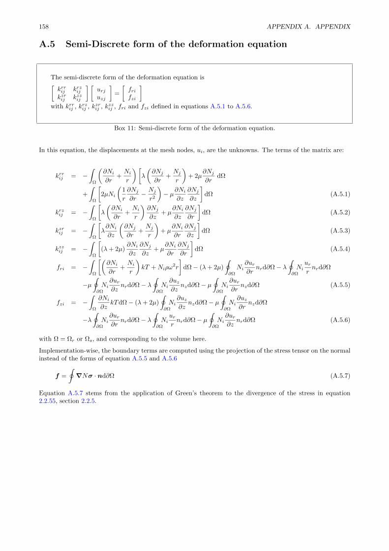
158 APPENDIX A. APPENDIX
A.5 Semi-Discrete form of the deformation equation
The semi-discrete form of the deformation equation is[krrij krzijkzrij kzzij
] [urjuzj
]=
[frifzi
]with krrij , krzij , kzrij , kzzij , fri and fzi defined in equations A.5.1 to A.5.6.
Box 11: Semi-discrete form of the deformation equation.
In this equation, the displacements at the mesh nodes, ui, are the unknowns. The terms of the matrix are:
krrij = −∫
Ω
(∂Ni∂r
+Nir
)[λ
(∂Nj∂r
+Njr
)+ 2µ
∂Nj∂r
dΩ
+
∫Ω
[2µNi
(1
r
∂Nj∂r− Njr2
)− µ∂Ni
∂z
∂Nj∂z
]dΩ (A.5.1)
krzij = −∫
Ω
[λ
(∂Ni∂r
+Nir
)∂Nj∂z
+ µ∂Ni∂z
∂Nj∂r
]dΩ (A.5.2)
kzrij = −∫
Ω
[λ∂Ni∂z
(∂Nj∂r
+Njr
)+ µ
∂Ni∂r
∂Nj∂z
]dΩ (A.5.3)
kzzij = −∫
Ω
[(λ+ 2µ)
∂Ni∂z
∂Nj∂z
+ µ∂Ni∂r
∂Nj∂r
]dΩ (A.5.4)
fri = −∫
Ω
[(∂Ni∂r
+Nir
)kT +Niρω
2r
]dΩ− (λ+ 2µ)
∮∂Ω
Ni∂ur∂r
nrd∂Ω− λ∮∂Ω
Niurrnrd∂Ω
−µ∮∂Ω
Ni∂ur∂z
nrd∂Ω− λ∮∂Ω
Ni∂uz∂z
nzd∂Ω− µ∮∂Ω
Ni∂ur∂r
nzd∂Ω (A.5.5)
fzi = −∫
Ω
∂Ni∂z
kTdΩ− (λ+ 2µ)
∮∂Ω
Ni∂uz∂z
nzd∂Ω− µ∮∂Ω
Ni∂uz∂r
nzd∂Ω
−λ∮∂Ω
Ni∂ur∂r
nrd∂Ω− λ∮∂Ω
Niurrnrd∂Ω− µ
∮∂Ω
Ni∂ur∂z
nrd∂Ω (A.5.6)
with Ω = Ωr or Ωs, and corresponding to the volume here.
Implementation-wise, the boundary terms are computed using the projection of the stress tensor on the normalinstead of the forms of equation A.5.5 and A.5.6
f =
∮∇Nσ · nd∂Ω (A.5.7)
Equation A.5.7 stems from the application of Green’s theorem to the divergence of the stress in equation2.2.55, section 2.2.5.
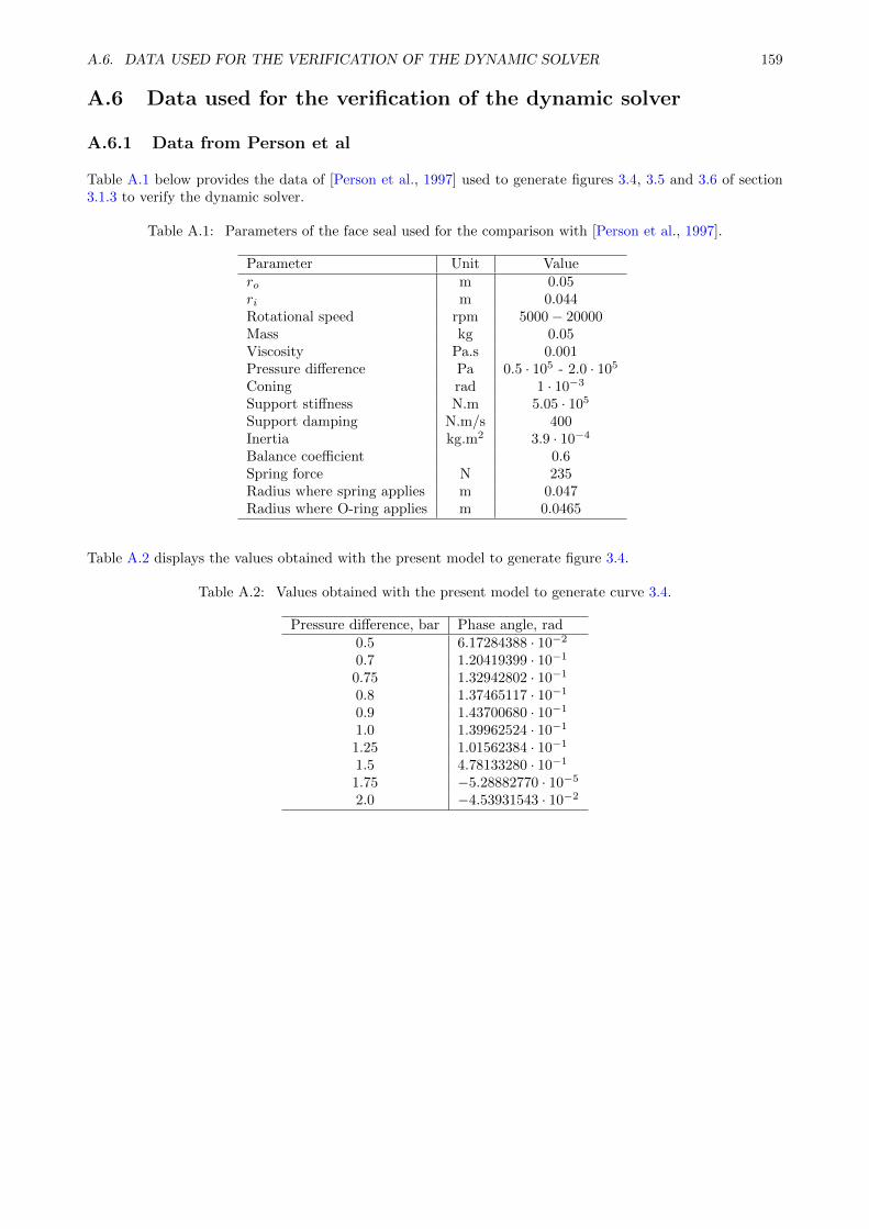
A.6. DATA USED FOR THE VERIFICATION OF THE DYNAMIC SOLVER 159
A.6 Data used for the verification of the dynamic solver
A.6.1 Data from Person et al
Table A.1 below provides the data of [Person et al., 1997] used to generate figures 3.4, 3.5 and 3.6 of section3.1.3 to verify the dynamic solver.
Table A.1: Parameters of the face seal used for the comparison with [Person et al., 1997].
Parameter Unit Valuero m 0.05ri m 0.044Rotational speed rpm 5000− 20000Mass kg 0.05Viscosity Pa.s 0.001Pressure difference Pa 0.5 · 105 - 2.0 · 105
Coning rad 1 · 10−3
Support stiffness N.m 5.05 · 105
Support damping N.m/s 400Inertia kg.m2 3.9 · 10−4
Balance coefficient 0.6Spring force N 235Radius where spring applies m 0.047Radius where O-ring applies m 0.0465
Table A.2 displays the values obtained with the present model to generate figure 3.4.
Table A.2: Values obtained with the present model to generate curve 3.4.
Pressure difference, bar Phase angle, rad0.5 6.17284388 · 10−2
0.7 1.20419399 · 10−1
0.75 1.32942802 · 10−1
0.8 1.37465117 · 10−1
0.9 1.43700680 · 10−1
1.0 1.39962524 · 10−1
1.25 1.01562384 · 10−1
1.5 4.78133280 · 10−1
1.75 −5.28882770 · 10−5
2.0 −4.53931543 · 10−2
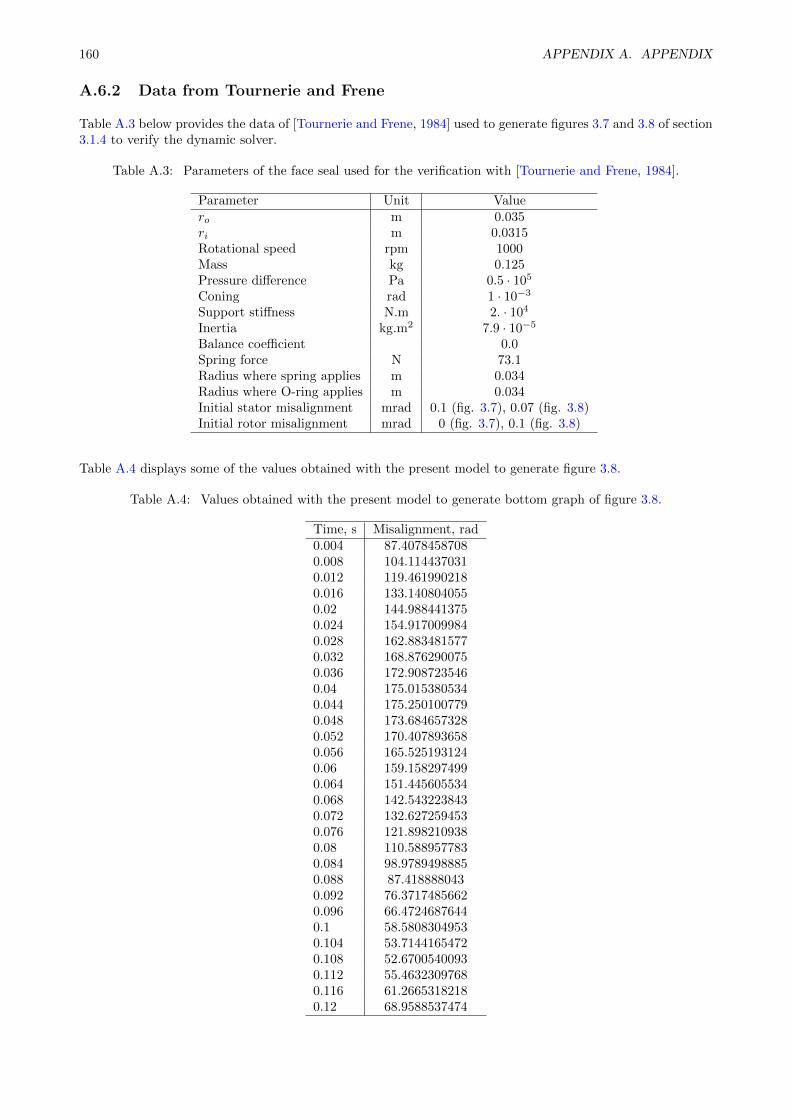
160 APPENDIX A. APPENDIX
A.6.2 Data from Tournerie and Frene
Table A.3 below provides the data of [Tournerie and Frene, 1984] used to generate figures 3.7 and 3.8 of section3.1.4 to verify the dynamic solver.
Table A.3: Parameters of the face seal used for the verification with [Tournerie and Frene, 1984].
Parameter Unit Valuero m 0.035ri m 0.0315Rotational speed rpm 1000Mass kg 0.125Pressure difference Pa 0.5 · 105
Coning rad 1 · 10−3
Support stiffness N.m 2. · 104
Inertia kg.m2 7.9 · 10−5
Balance coefficient 0.0Spring force N 73.1Radius where spring applies m 0.034Radius where O-ring applies m 0.034Initial stator misalignment mrad 0.1 (fig. 3.7), 0.07 (fig. 3.8)Initial rotor misalignment mrad 0 (fig. 3.7), 0.1 (fig. 3.8)
Table A.4 displays some of the values obtained with the present model to generate figure 3.8.
Table A.4: Values obtained with the present model to generate bottom graph of figure 3.8.
Time, s Misalignment, rad0.004 87.40784587080.008 104.1144370310.012 119.4619902180.016 133.1408040550.02 144.9884413750.024 154.9170099840.028 162.8834815770.032 168.8762900750.036 172.9087235460.04 175.0153805340.044 175.2501007790.048 173.6846573280.052 170.4078936580.056 165.5251931240.06 159.1582974990.064 151.4456055340.068 142.5432238430.072 132.6272594530.076 121.8982109380.08 110.5889577830.084 98.97894988850.088 87.4188880430.092 76.37174856620.096 66.47246876440.1 58.58083049530.104 53.71441654720.108 52.67005400930.112 55.46323097680.116 61.26653182180.12 68.9588537474
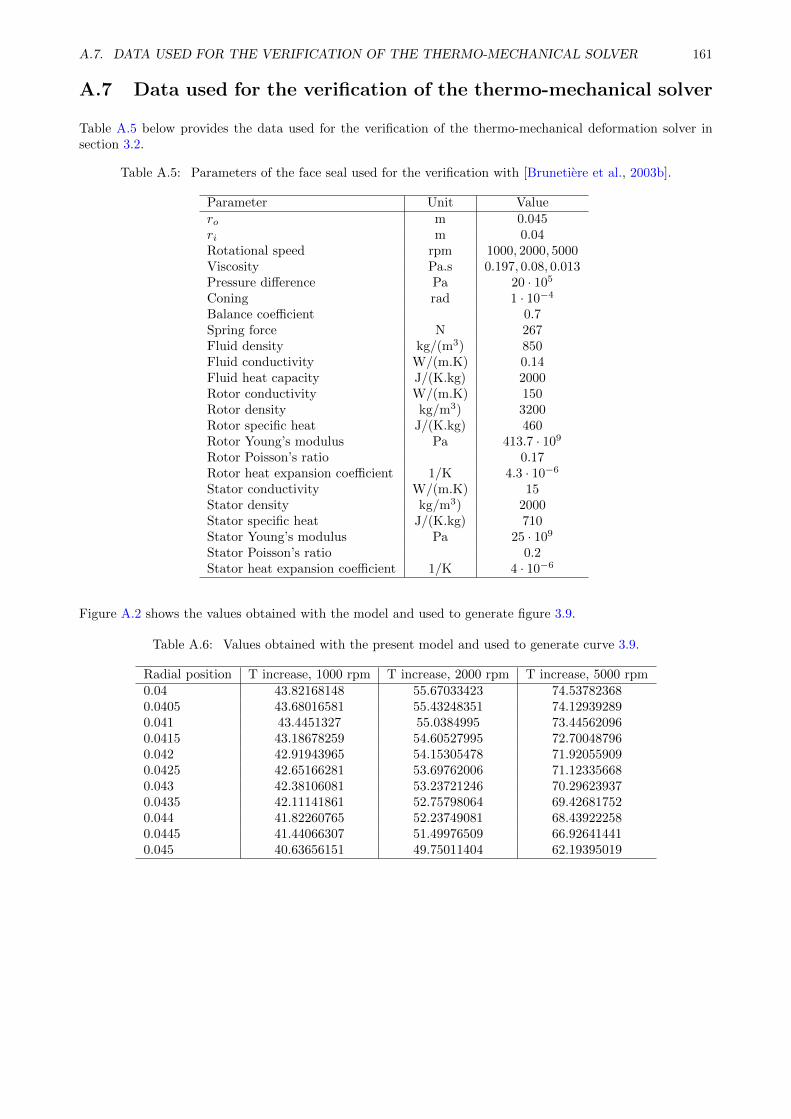
A.7. DATA USED FOR THE VERIFICATION OF THE THERMO-MECHANICAL SOLVER 161
A.7 Data used for the verification of the thermo-mechanical solver
Table A.5 below provides the data used for the verification of the thermo-mechanical deformation solver insection 3.2.
Table A.5: Parameters of the face seal used for the verification with [Brunetiere et al., 2003b].
Parameter Unit Valuero m 0.045ri m 0.04Rotational speed rpm 1000, 2000, 5000Viscosity Pa.s 0.197, 0.08, 0.013Pressure difference Pa 20 · 105
Coning rad 1 · 10−4
Balance coefficient 0.7Spring force N 267Fluid density kg/(m3) 850Fluid conductivity W/(m.K) 0.14Fluid heat capacity J/(K.kg) 2000Rotor conductivity W/(m.K) 150Rotor density kg/m3) 3200Rotor specific heat J/(K.kg) 460Rotor Young’s modulus Pa 413.7 · 109
Rotor Poisson’s ratio 0.17Rotor heat expansion coefficient 1/K 4.3 · 10−6
Stator conductivity W/(m.K) 15Stator density kg/m3) 2000Stator specific heat J/(K.kg) 710Stator Young’s modulus Pa 25 · 109
Stator Poisson’s ratio 0.2Stator heat expansion coefficient 1/K 4 · 10−6
Figure A.2 shows the values obtained with the model and used to generate figure 3.9.
Table A.6: Values obtained with the present model and used to generate curve 3.9.
Radial position T increase, 1000 rpm T increase, 2000 rpm T increase, 5000 rpm0.04 43.82168148 55.67033423 74.537823680.0405 43.68016581 55.43248351 74.129392890.041 43.4451327 55.0384995 73.445620960.0415 43.18678259 54.60527995 72.700487960.042 42.91943965 54.15305478 71.920559090.0425 42.65166281 53.69762006 71.123356680.043 42.38106081 53.23721246 70.296239370.0435 42.11141861 52.75798064 69.426817520.044 41.82260765 52.23749081 68.439222580.0445 41.44066307 51.49976509 66.926414410.045 40.63656151 49.75011404 62.19395019
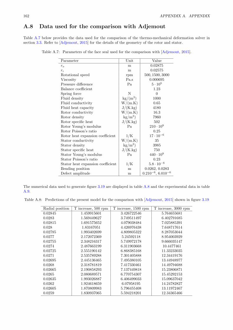
162 APPENDIX A. APPENDIX
A.8 Data used for the comparison with Adjemout
Table A.7 below provides the data used for the comparison of the thermo-mechanical deformation solver insection 3.3. Refer to [Adjemout, 2015] for the details of the geometry of the rotor and stator.
Table A.7: Parameters of the face seal used for the comparison with [Adjemout, 2015].
Parameter Unit Valuero m 0.02875ri m 0.02575Rotational speed rpm 500, 1500, 3000Viscosity Pa.s 0.000695Pressure difference Pa 5 · 105
Balance coefficient 1.23Spring force N 0Fluid density kg/(m3) 1000Fluid conductivity W/(m.K) 0.65Fluid heat capacity J/(K.kg) 4180Rotor conductivity W/(m.K) 16.3Rotor density kg/m3) 7960Rotor specific heat J/(K.kg) 502Rotor Young’s modulus Pa 210 · 109
Rotor Poisson’s ratio 0.25Rotor heat expansion coefficient 1/K 17 · 10−6
Stator conductivity W/(m.K) 35Stator density kg/m3) 3985Stator specific heat J/(K.kg) 750Stator Young’s modulus Pa 440 · 109
Stator Poisson’s ratio 0.23Stator heat expansion coefficient 1/K 5.8 · 10−6
Bending position m 0.0262, 0.0283Defect amplitude m 0.210−6, 6.010−6
The numerical data used to generate figure 3.19 are displayed in table A.8 and the experimental data in tableA.9.
Table A.8: Predictions of the present model for the comparison with [Adjemout, 2015] shown in figure 3.19
Radial position T increase, 500 rpm T increase, 1500 rpm T increase, 3000 rpm0.02845 1.459915601 3.426722546 5.7646556810.0283 1.569449627 3.749511497 6.4027916850.02815 1.691575652 4.079038484 7.0258853910.028 1.83167051 4.426976438 7.6487176140.02785 1.993402699 4.809805322 8.2870530440.0277 2.172072369 5.24592118 8.9540039290.02755 2.348216317 5.749972178 9.6660351470.0274 2.487663199 6.311903668 10.44774610.02725 2.555190142 6.868385168 11.332330350.0271 2.535789288 7.301405888 12.344191760.02695 2.445136465 7.495380105 13.449489770.0268 2.318781819 7.417330461 14.497946880.02665 2.190858293 7.137449818 15.238068710.0265 2.080689571 6.770754307 15.452921530.02635 1.993026887 6.406499033 15.096370420.0262 1.924618659 6.07958195 14.247828270.02605 1.870809983 5.796455408 13.119724670.0259 1.830937065 5.594218201 12.34365466
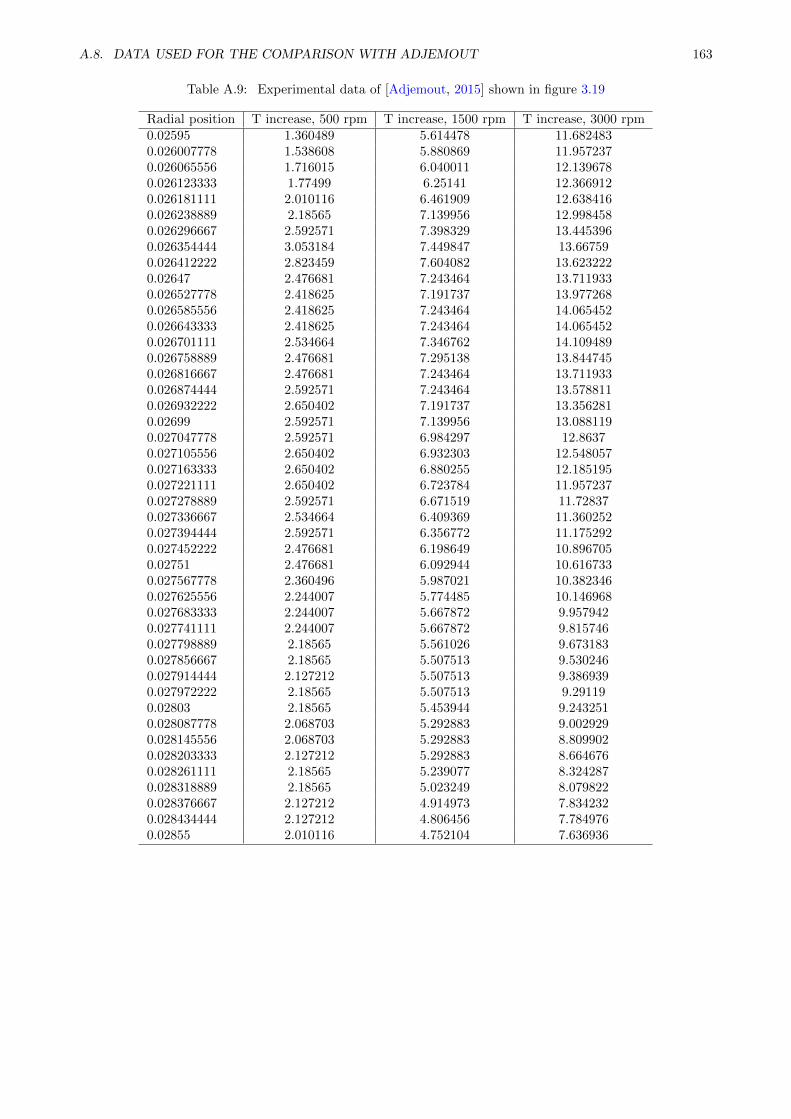
A.8. DATA USED FOR THE COMPARISON WITH ADJEMOUT 163
Table A.9: Experimental data of [Adjemout, 2015] shown in figure 3.19
Radial position T increase, 500 rpm T increase, 1500 rpm T increase, 3000 rpm0.02595 1.360489 5.614478 11.6824830.026007778 1.538608 5.880869 11.9572370.026065556 1.716015 6.040011 12.1396780.026123333 1.77499 6.25141 12.3669120.026181111 2.010116 6.461909 12.6384160.026238889 2.18565 7.139956 12.9984580.026296667 2.592571 7.398329 13.4453960.026354444 3.053184 7.449847 13.667590.026412222 2.823459 7.604082 13.6232220.02647 2.476681 7.243464 13.7119330.026527778 2.418625 7.191737 13.9772680.026585556 2.418625 7.243464 14.0654520.026643333 2.418625 7.243464 14.0654520.026701111 2.534664 7.346762 14.1094890.026758889 2.476681 7.295138 13.8447450.026816667 2.476681 7.243464 13.7119330.026874444 2.592571 7.243464 13.5788110.026932222 2.650402 7.191737 13.3562810.02699 2.592571 7.139956 13.0881190.027047778 2.592571 6.984297 12.86370.027105556 2.650402 6.932303 12.5480570.027163333 2.650402 6.880255 12.1851950.027221111 2.650402 6.723784 11.9572370.027278889 2.592571 6.671519 11.728370.027336667 2.534664 6.409369 11.3602520.027394444 2.592571 6.356772 11.1752920.027452222 2.476681 6.198649 10.8967050.02751 2.476681 6.092944 10.6167330.027567778 2.360496 5.987021 10.3823460.027625556 2.244007 5.774485 10.1469680.027683333 2.244007 5.667872 9.9579420.027741111 2.244007 5.667872 9.8157460.027798889 2.18565 5.561026 9.6731830.027856667 2.18565 5.507513 9.5302460.027914444 2.127212 5.507513 9.3869390.027972222 2.18565 5.507513 9.291190.02803 2.18565 5.453944 9.2432510.028087778 2.068703 5.292883 9.0029290.028145556 2.068703 5.292883 8.8099020.028203333 2.127212 5.292883 8.6646760.028261111 2.18565 5.239077 8.3242870.028318889 2.18565 5.023249 8.0798220.028376667 2.127212 4.914973 7.8342320.028434444 2.127212 4.806456 7.7849760.02855 2.010116 4.752104 7.636936
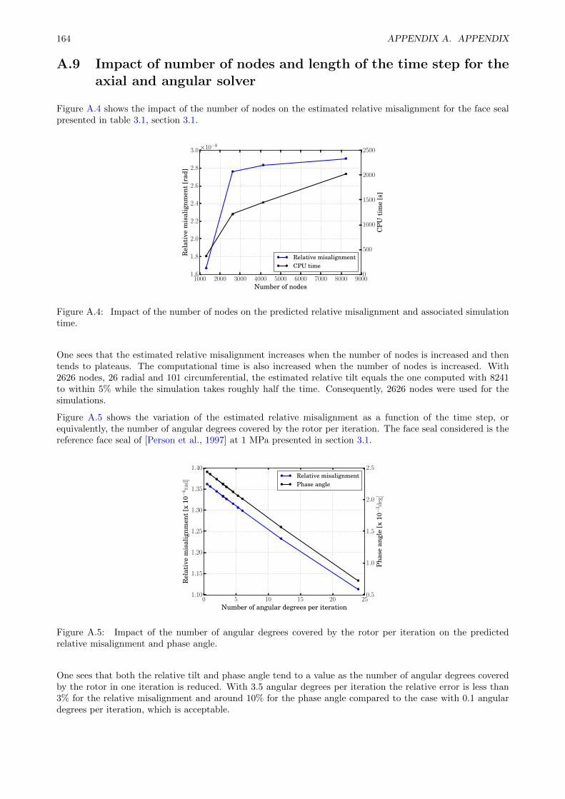
164 APPENDIX A. APPENDIX
A.9 Impact of number of nodes and length of the time step for theaxial and angular solver
Figure A.4 shows the impact of the number of nodes on the estimated relative misalignment for the face sealpresented in table 3.1, section 3.1.
1000 2000 3000 4000 5000 6000 7000 8000 9000Number of nodes
1.6
1.8
2.0
2.2
2.4
2.6
2.8
3.0
Rel
ativ
em
isal
ignm
ent
[rad
]
×10−8
Relative misalignmentCPU time
0
500
1000
1500
2000
2500
CP
Uti
me
[s]
Figure A.4: Impact of the number of nodes on the predicted relative misalignment and associated simulationtime.
One sees that the estimated relative misalignment increases when the number of nodes is increased and thentends to plateaus. The computational time is also increased when the number of nodes is increased. With2626 nodes, 26 radial and 101 circumferential, the estimated relative tilt equals the one computed with 8241to within 5% while the simulation takes roughly half the time. Consequently, 2626 nodes were used for thesimulations.
Figure A.5 shows the variation of the estimated relative misalignment as a function of the time step, orequivalently, the number of angular degrees covered by the rotor per iteration. The face seal considered is thereference face seal of [Person et al., 1997] at 1 MPa presented in section 3.1.
0 5 10 15 20 25Number of angular degrees per iteration
1.10
1.15
1.20
1.25
1.30
1.35
1.40
Rel
ativ
em
isal
ignm
ent
[x10−
6ra
d] Relative misalignment
Phase angle
0.5
1.0
1.5
2.0
2.5
Pha
sean
gle
[x10−
3d
eg]
Figure A.5: Impact of the number of angular degrees covered by the rotor per iteration on the predictedrelative misalignment and phase angle.
One sees that both the relative tilt and phase angle tend to a value as the number of angular degrees coveredby the rotor in one iteration is reduced. With 3.5 angular degrees per iteration the relative error is less than3% for the relative misalignment and around 10% for the phase angle compared to the case with 0.1 angulardegrees per iteration, which is acceptable.
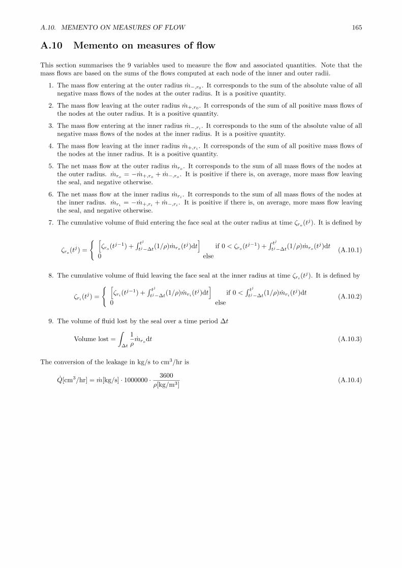
A.10. MEMENTO ON MEASURES OF FLOW 165
A.10 Memento on measures of flow
This section summarises the 9 variables used to measure the flow and associated quantities. Note that themass flows are based on the sums of the flows computed at each node of the inner and outer radii.
1. The mass flow entering at the outer radius m−,r0 . It corresponds to the sum of the absolute value of allnegative mass flows of the nodes at the outer radius. It is a positive quantity.
2. The mass flow leaving at the outer radius m+,r0 . It corresponds of the sum of all positive mass flows ofthe nodes at the outer radius. It is a positive quantity.
3. The mass flow entering at the inner radius m−,ri . It corresponds to the sum of the absolute value of allnegative mass flows of the nodes at the inner radius. It is a positive quantity.
4. The mass flow leaving at the inner radius m+,ri . It corresponds of the sum of all positive mass flows ofthe nodes at the inner radius. It is a positive quantity.
5. The net mass flow at the outer radius mro . It corresponds to the sum of all mass flows of the nodes atthe outer radius. mro = −m+,ro + m−,ro . It is positive if there is, on average, more mass flow leavingthe seal, and negative otherwise.
6. The net mass flow at the inner radius mri . It corresponds to the sum of all mass flows of the nodes atthe inner radius. mri = −m+,ri + m−,ri . It is positive if there is, on average, more mass flow leavingthe seal, and negative otherwise.
7. The cumulative volume of fluid entering the face seal at the outer radius at time ζro(tj). It is defined by
ζro(tj) =
[ζro(tj−1) +
∫ tjtj−∆t
(1/ρ)mro(tj)dt]
if 0 < ζro(tj−1) +∫ tjtj−∆t
(1/ρ)mro(tj)dt
0 else(A.10.1)
8. The cumulative volume of fluid leaving the face seal at the inner radius at time ζri(tj). It is defined by
ζri(tj) =
[ζri(t
j−1) +∫ tjtj−∆t
(1/ρ)mri(tj)dt
]if 0 <
∫ tjtj−∆t
(1/ρ)mri(tj)dt
0 else(A.10.2)
9. The volume of fluid lost by the seal over a time period ∆t
Volume lost =
∫∆t
1
ρmrodt (A.10.3)
The conversion of the leakage in kg/s to cm3/hr is
Q[cm3/hr] = m[kg/s] · 1000000 · 3600
ρ[kg/m3](A.10.4)
166 APPENDIX A. APPENDIX
A.11 Additional measurements investigated
This section presents other measurements contemplated for the experimental setup but that could not beimplemented or provided limited results.
A.11.1 Seal temperature measurement
It is desirable to monitor the face seal temperature during the test, especially during start-ups. Three mea-surements were contemplated:
measurement of the rotor temperature;
measurement of stator temperature;
measurement of the fluid temperature in the vicinity of the face seal.
Measurement of rotor temperature The idea considered was to glue a thermocouple on the rotor’slateral or rear face and to connect it to a transmitter located on the rotating shaft. The measurement wouldbe sent via high frequency waves to a receiver located outside of the pressure cell. This measurement couldnot be implemented due to space limitations and the absence of commercially available transmitters operatingin water.
Measurement of stator temperature The idea was to glue a thermocouple or PT100 sensor to a part ofthe stator located in the oil. The thermo-couple wires would then be placed inside the face seal holder andexit through a feedthrough. This could not be implemented due to the limited space around the stator.
Measurement of temperature at the vicinity of the face seal The idea was to place a thermo-couplein the water along the face seal holder and to position its temperature-sensing end close to the outer radiusof the stator. Although this second idea was implemented, the thermo-couple end could not be placed closeenough to the stator to record any valuable data; this measurement was subsequently abandoned.
A.11.2 Torque measurement
A torque meter located between the motor and the female magnetic coupling was originally present in thesetup. The torque meter broke, as it was not capable of withstanding the shaft temperature resulting fromcontinuous operation of the setup at 3500 rpm. The torque measurement was replaced by a measurementof the drive intensity calibrated using another torque meter. The torque measurement includes the variouselement of the shaft: bearings, magnetic coupling, fluid friction around the seal. As such, only average andqualitative information about the face seal torque could be obtained.
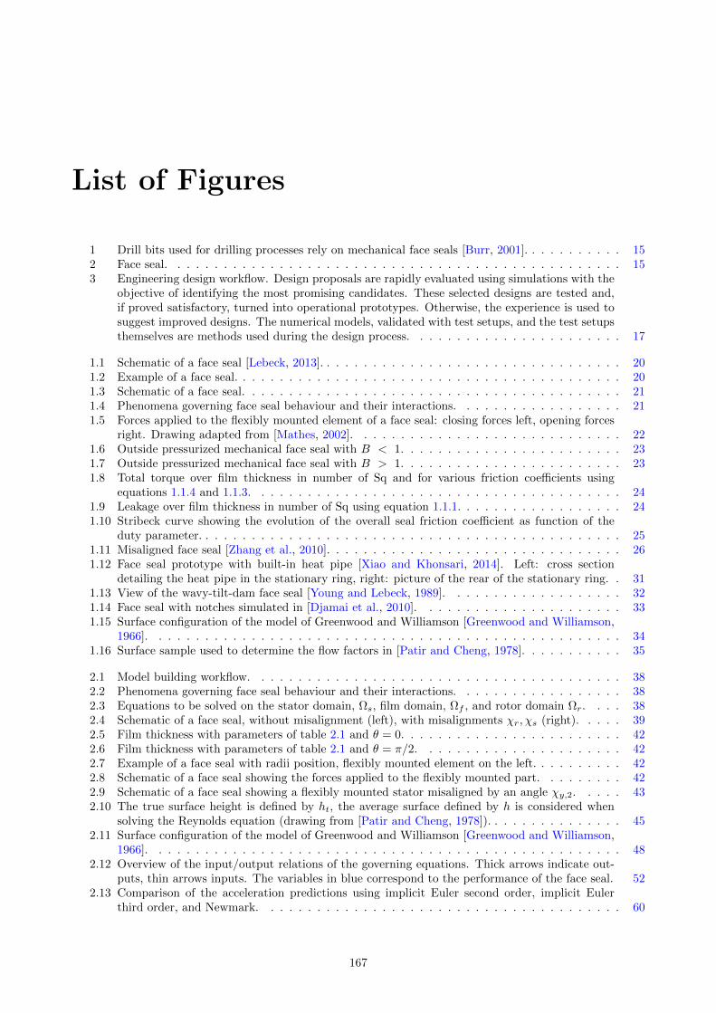
List of Figures
1 Drill bits used for drilling processes rely on mechanical face seals [Burr, 2001]. . . . . . . . . . . 152 Face seal. . . . . . . . . . . . . . . . . . . . . . . . . . . . . . . . . . . . . . . . . . . . . . . . . 153 Engineering design workflow. Design proposals are rapidly evaluated using simulations with the
objective of identifying the most promising candidates. These selected designs are tested and,if proved satisfactory, turned into operational prototypes. Otherwise, the experience is used tosuggest improved designs. The numerical models, validated with test setups, and the test setupsthemselves are methods used during the design process. . . . . . . . . . . . . . . . . . . . . . . 17
1.1 Schematic of a face seal [Lebeck, 2013]. . . . . . . . . . . . . . . . . . . . . . . . . . . . . . . . . 201.2 Example of a face seal. . . . . . . . . . . . . . . . . . . . . . . . . . . . . . . . . . . . . . . . . . 201.3 Schematic of a face seal. . . . . . . . . . . . . . . . . . . . . . . . . . . . . . . . . . . . . . . . . 211.4 Phenomena governing face seal behaviour and their interactions. . . . . . . . . . . . . . . . . . 211.5 Forces applied to the flexibly mounted element of a face seal: closing forces left, opening forces
right. Drawing adapted from [Mathes, 2002]. . . . . . . . . . . . . . . . . . . . . . . . . . . . . 221.6 Outside pressurized mechanical face seal with B < 1. . . . . . . . . . . . . . . . . . . . . . . . 231.7 Outside pressurized mechanical face seal with B > 1. . . . . . . . . . . . . . . . . . . . . . . . 231.8 Total torque over film thickness in number of Sq and for various friction coefficients using
equations 1.1.4 and 1.1.3. . . . . . . . . . . . . . . . . . . . . . . . . . . . . . . . . . . . . . . . 241.9 Leakage over film thickness in number of Sq using equation 1.1.1. . . . . . . . . . . . . . . . . . 241.10 Stribeck curve showing the evolution of the overall seal friction coefficient as function of the
duty parameter. . . . . . . . . . . . . . . . . . . . . . . . . . . . . . . . . . . . . . . . . . . . . . 251.11 Misaligned face seal [Zhang et al., 2010]. . . . . . . . . . . . . . . . . . . . . . . . . . . . . . . . 261.12 Face seal prototype with built-in heat pipe [Xiao and Khonsari, 2014]. Left: cross section
detailing the heat pipe in the stationary ring, right: picture of the rear of the stationary ring. . 311.13 View of the wavy-tilt-dam face seal [Young and Lebeck, 1989]. . . . . . . . . . . . . . . . . . . 321.14 Face seal with notches simulated in [Djamai et al., 2010]. . . . . . . . . . . . . . . . . . . . . . 331.15 Surface configuration of the model of Greenwood and Williamson [Greenwood and Williamson,
1966]. . . . . . . . . . . . . . . . . . . . . . . . . . . . . . . . . . . . . . . . . . . . . . . . . . . 341.16 Surface sample used to determine the flow factors in [Patir and Cheng, 1978]. . . . . . . . . . . 35
2.1 Model building workflow. . . . . . . . . . . . . . . . . . . . . . . . . . . . . . . . . . . . . . . . 382.2 Phenomena governing face seal behaviour and their interactions. . . . . . . . . . . . . . . . . . 382.3 Equations to be solved on the stator domain, Ωs, film domain, Ωf , and rotor domain Ωr. . . . 382.4 Schematic of a face seal, without misalignment (left), with misalignments χr, χs (right). . . . . 392.5 Film thickness with parameters of table 2.1 and θ = 0. . . . . . . . . . . . . . . . . . . . . . . . 422.6 Film thickness with parameters of table 2.1 and θ = π/2. . . . . . . . . . . . . . . . . . . . . . 422.7 Example of a face seal with radii position, flexibly mounted element on the left. . . . . . . . . . 422.8 Schematic of a face seal showing the forces applied to the flexibly mounted part. . . . . . . . . 422.9 Schematic of a face seal showing a flexibly mounted stator misaligned by an angle χy,2. . . . . 432.10 The true surface height is defined by ht, the average surface defined by h is considered when
solving the Reynolds equation (drawing from [Patir and Cheng, 1978]). . . . . . . . . . . . . . . 452.11 Surface configuration of the model of Greenwood and Williamson [Greenwood and Williamson,
1966]. . . . . . . . . . . . . . . . . . . . . . . . . . . . . . . . . . . . . . . . . . . . . . . . . . . 482.12 Overview of the input/output relations of the governing equations. Thick arrows indicate out-
puts, thin arrows inputs. The variables in blue correspond to the performance of the face seal. 522.13 Comparison of the acceleration predictions using implicit Euler second order, implicit Euler
third order, and Newmark. . . . . . . . . . . . . . . . . . . . . . . . . . . . . . . . . . . . . . . 60
167
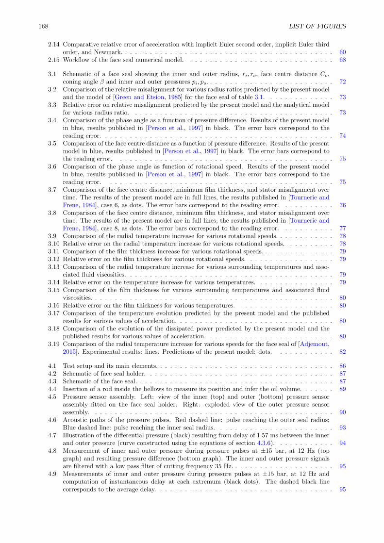
168 LIST OF FIGURES
2.14 Comparative relative error of acceleration with implicit Euler second order, implicit Euler thirdorder, and Newmark. . . . . . . . . . . . . . . . . . . . . . . . . . . . . . . . . . . . . . . . . . . 60
2.15 Workflow of the face seal numerical model. . . . . . . . . . . . . . . . . . . . . . . . . . . . . . 68
3.1 Schematic of a face seal showing the inner and outer radius, ri, ro, face centre distance Co,coning angle β and inner and outer pressures pi, po. . . . . . . . . . . . . . . . . . . . . . . . . . 72
3.2 Comparison of the relative misalignment for various radius ratios predicted by the present modeland the model of [Green and Etsion, 1985] for the face seal of table 3.1. . . . . . . . . . . . . . 73
3.3 Relative error on relative misalignment predicted by the present model and the analytical modelfor various radius ratio. . . . . . . . . . . . . . . . . . . . . . . . . . . . . . . . . . . . . . . . . 73
3.4 Comparison of the phase angle as a function of pressure difference. Results of the present modelin blue, results published in [Person et al., 1997] in black. The error bars correspond to thereading error. . . . . . . . . . . . . . . . . . . . . . . . . . . . . . . . . . . . . . . . . . . . . . . 74
3.5 Comparison of the face centre distance as a function of pressure difference. Results of the presentmodel in blue, results published in [Person et al., 1997] in black. The error bars correspond tothe reading error. . . . . . . . . . . . . . . . . . . . . . . . . . . . . . . . . . . . . . . . . . . . 75
3.6 Comparison of the phase angle as function of rotational speed. Results of the present modelin blue, results published in [Person et al., 1997] in black. The error bars correspond to thereading error. . . . . . . . . . . . . . . . . . . . . . . . . . . . . . . . . . . . . . . . . . . . . . 75
3.7 Comparison of the face centre distance, minimum film thickness, and stator misalignment overtime. The results of the present model are in full lines, the results published in [Tournerie andFrene, 1984], case 6, as dots. The error bars correspond to the reading error. . . . . . . . . . . 76
3.8 Comparison of the face centre distance, minimum film thickness, and stator misalignment overtime. The results of the present model are in full lines; the results published in [Tournerie andFrene, 1984], case 8, as dots. The error bars correspond to the reading error. . . . . . . . . . . 77
3.9 Comparison of the radial temperature increase for various rotational speeds. . . . . . . . . . . . 783.10 Relative error on the radial temperature increase for various rotational speeds. . . . . . . . . . 783.11 Comparison of the film thickness increase for various rotational speeds. . . . . . . . . . . . . . . 793.12 Relative error on the film thickness for various rotational speeds. . . . . . . . . . . . . . . . . . 793.13 Comparison of the radial temperature increase for various surrounding temperatures and asso-
ciated fluid viscosities. . . . . . . . . . . . . . . . . . . . . . . . . . . . . . . . . . . . . . . . . . 793.14 Relative error on the temperature increase for various temperatures. . . . . . . . . . . . . . . . 793.15 Comparison of the film thickness for various surrounding temperatures and associated fluid
viscosities. . . . . . . . . . . . . . . . . . . . . . . . . . . . . . . . . . . . . . . . . . . . . . . . . 803.16 Relative error on the film thickness for various temperatures. . . . . . . . . . . . . . . . . . . . 803.17 Comparison of the temperature evolution predicted by the present model and the published
results for various values of acceleration. . . . . . . . . . . . . . . . . . . . . . . . . . . . . . . . 803.18 Comparison of the evolution of the dissipated power predicted by the present model and the
published results for various values of acceleration. . . . . . . . . . . . . . . . . . . . . . . . . . 803.19 Comparison of the radial temperature increase for various speeds for the face seal of [Adjemout,
2015]. Experimental results: lines. Predictions of the present model: dots. . . . . . . . . . . . 82
4.1 Test setup and its main elements. . . . . . . . . . . . . . . . . . . . . . . . . . . . . . . . . . . . 864.2 Schematic of face seal holder. . . . . . . . . . . . . . . . . . . . . . . . . . . . . . . . . . . . . . 874.3 Schematic of the face seal. . . . . . . . . . . . . . . . . . . . . . . . . . . . . . . . . . . . . . . . 874.4 Insertion of a rod inside the bellows to measure its position and infer the oil volume. . . . . . . 894.5 Pressure sensor assembly. Left: view of the inner (top) and outer (bottom) pressure sensor
assembly fitted on the face seal holder. Right: exploded view of the outer pressure sensorassembly. . . . . . . . . . . . . . . . . . . . . . . . . . . . . . . . . . . . . . . . . . . . . . . . . 90
4.6 Acoustic paths of the pressure pulses. Red dashed line: pulse reaching the outer seal radius;Blue dashed line: pulse reaching the inner seal radius. . . . . . . . . . . . . . . . . . . . . . . . 93
4.7 Illustration of the differential pressure (black) resulting from delay of 1.57 ms between the innerand outer pressure (curve constructed using the equations of section 4.3.6). . . . . . . . . . . . 94
4.8 Measurement of inner and outer pressure during pressure pulses at ±15 bar, at 12 Hz (topgraph) and resulting pressure difference (bottom graph). The inner and outer pressure signalsare filtered with a low pass filter of cutting frequency 35 Hz. . . . . . . . . . . . . . . . . . . . . 95
4.9 Measurements of inner and outer pressure during pressure pulses at ±15 bar, at 12 Hz andcomputation of instantaneous delay at each extremum (black dots). The dashed black linecorresponds to the average delay. . . . . . . . . . . . . . . . . . . . . . . . . . . . . . . . . . . . 95
LIST OF FIGURES 169
5.1 Geometry of the face seal of interest. . . . . . . . . . . . . . . . . . . . . . . . . . . . . . . . . 1005.2 Schematic of the face seal and its surroundings. . . . . . . . . . . . . . . . . . . . . . . . . . . . 1005.3 Temperature increase (colour map) in the face seal at reference conditions with isotherms (lines)
and deformations magnified 1000 times. . . . . . . . . . . . . . . . . . . . . . . . . . . . . . . . 1025.4 Radial film temperature and film thickness profiles of the face seal at reference conditions. . . . 1025.5 Radial distributions of the contact and fluid pressure contributions for the face seal at reference
conditions. . . . . . . . . . . . . . . . . . . . . . . . . . . . . . . . . . . . . . . . . . . . . . . . . 1035.6 Convection coefficient for oil, water and resulting face seal leakage and maximum fluid temper-
ature increase for various correlations of convection coefficient. . . . . . . . . . . . . . . . . . . 1055.7 Impact of the friction coefficient. . . . . . . . . . . . . . . . . . . . . . . . . . . . . . . . . . . . 1065.8 Impact of the surface asperity standard roughness with λ = 1.78 µm. . . . . . . . . . . . . . . . 1075.9 Impact of the surface correlation length with Sq = 0.18 µm. . . . . . . . . . . . . . . . . . . . . 1075.10 Impact of the operating temperature on the performance of the reference face seal. . . . . . . . 1085.11 Impact of the rotational speed on the performance of the reference face seal. . . . . . . . . . . . 1095.12 Impact of the spring force on the performance of the reference face seal. . . . . . . . . . . . . . 1095.13 Impact of the acceleration on the dissipated power, torque, leakage, maximum temperature
increase, minimum and maximum film thickness. . . . . . . . . . . . . . . . . . . . . . . . . . . 1115.14 Leakage and torque of the reference face seal for various numbers of nodes at the interface. . . 1125.15 Impact of the pressure pulses (top graph) on the mass flows (middle graph), minimum film thick-
ness and maximum contact pressure (bottom graph). Simulation performed with the referenceconditions and pressure pulses. . . . . . . . . . . . . . . . . . . . . . . . . . . . . . . . . . . . . 115
5.16 Evolution of the film thickness (left), fluid pressure (middle) and contact pressure (right) of thereference face seal during pressure pulses. . . . . . . . . . . . . . . . . . . . . . . . . . . . . . . 116
5.17 Radial film fluid pressure during pulses at various time instants. . . . . . . . . . . . . . . . . . 1175.18 Radial film thickness profile during pulses at various time instants. . . . . . . . . . . . . . . . . 1175.19 Radial contact pressure profile during pulses at various time instants. . . . . . . . . . . . . . . 1175.20 Illustration of the variation of ζr0(tj)/V (tj) (eq. 5.3.2) when the water travels 0%, 23% and
72% of the sealing dam (from left to right). . . . . . . . . . . . . . . . . . . . . . . . . . . . . . 1185.21 Time evolution of the volume travelled by the fluid at the outer [ζro/V (t) (eq. 5.3.2)] and inner
[ζri/V (t) (eq. 5.3.3)] radius. . . . . . . . . . . . . . . . . . . . . . . . . . . . . . . . . . . . . . . 1195.22 Impact of the surface wear on the minimum film thickness and maximum contact pressure . . . 1205.23 Impact of the surface wear on the maximum percentage of volume travelled by the water . . . 1205.24 Impact of the surface wear on the leakage . . . . . . . . . . . . . . . . . . . . . . . . . . . . . . 1205.25 View of the face misalignment and phase angle. . . . . . . . . . . . . . . . . . . . . . . . . . . . 1245.26 Impact of the rotor misalignment on the leakage and torque. . . . . . . . . . . . . . . . . . . . 1245.27 Impact of the rotor misalignment on the relative misalignment and phase angle. . . . . . . . . . 1245.28 Evolution of the film thickness (left), fluid pressure (middle) and contact pressure (right) during
the seal rotation when the rotor has 3 mrad misalignment. . . . . . . . . . . . . . . . . . . . . . 1255.29 Impact of the misalignment on the mass flows entering and exiting the seal at the outer (top)
and inner (bottom) radii. . . . . . . . . . . . . . . . . . . . . . . . . . . . . . . . . . . . . . . . 1265.30 Impact of the rotor misalignment χr on the maximum contact pressure and minimum film
thickness. . . . . . . . . . . . . . . . . . . . . . . . . . . . . . . . . . . . . . . . . . . . . . . . . 1275.31 Pressure boundary condition, mass flows at the inner and outer radius, percentage seal volume
travelled, minimum film thickness and maximum contact pressure for a face seal with a rotormisalignment of 3.5 mrad. . . . . . . . . . . . . . . . . . . . . . . . . . . . . . . . . . . . . . . 128
5.32 Surface defect of the diamond face seal prototype, left: rotor, right: stator. . . . . . . . . . . . 1305.33 View of a face of the face seal . . . . . . . . . . . . . . . . . . . . . . . . . . . . . . . . . . . . . 1325.34 Circumferential height profile taken at the mean radius of a face of a face seal. The height varies
between +0.4 and -0.4 µm. . . . . . . . . . . . . . . . . . . . . . . . . . . . . . . . . . . . . . . 1325.35 View of the position of the rotor and stator lobes as the rotor rotates. Fixed position of the
stator (black), position of the rotor when its lobes face the stator valleys (blue), position ofthe rotor after 45 degrees rotation (green) and after 90 degrees rotations (red). The distancebetween the rotor and stator is arbitrary. . . . . . . . . . . . . . . . . . . . . . . . . . . . . . . 133
5.36 Evolution of the mass flow, film thickness and maximum contact pressure for the reference faceseal with waviness. . . . . . . . . . . . . . . . . . . . . . . . . . . . . . . . . . . . . . . . . . . . 134
5.37 Time evolution of the the film thickness, film pressure and contact pressure over time. There isa 45 degrees rotation counter-clockwise between each row of figures, starting from the top row. 135
5.38 Composition of the mass flows for the reference face seal with a waviness defect of 0.5 µm onthe rotor and 0.4 µm on the stator. . . . . . . . . . . . . . . . . . . . . . . . . . . . . . . . . . . 137
170 LIST OF FIGURES
5.39 Simulation of the impact of the flatness defect on the leakage for the reference face seal (test 5was presented in table 5.14). . . . . . . . . . . . . . . . . . . . . . . . . . . . . . . . . . . . . . . 138
5.40 Simulation of the impact of the flatness defect on the maximum water ingression for the referenceface seal. . . . . . . . . . . . . . . . . . . . . . . . . . . . . . . . . . . . . . . . . . . . . . . . . . 138
5.41 Comparative impact of the average film thickness due to face waviness and surface roughnesson the leakage. . . . . . . . . . . . . . . . . . . . . . . . . . . . . . . . . . . . . . . . . . . . . . 139
5.42 Maximum contact force as a function of average flatness defect. . . . . . . . . . . . . . . . . . . 1405.43 Mass flows, percentage of seal volume travelled, maximum contact pressure and minimum film
thickness for the reference face seal with a waviness defect of 0.4 µm (stator) and 0.5 µm (rotor)operating with pressure pulses . . . . . . . . . . . . . . . . . . . . . . . . . . . . . . . . . . . . . 141
5.44 Mass flows, percentage of seal volume travelled, maximum contact pressure and minimum filmthickness for the diamond face seal of waviness 3.5 µm (stator) and 5.47 µm (rotor) operatingwith pressure pulses . . . . . . . . . . . . . . . . . . . . . . . . . . . . . . . . . . . . . . . . . . 143
A.1 Axis transformations. From left to right: face position, rotation, axial translation, first mis-alignment angle, second misalignment angle. . . . . . . . . . . . . . . . . . . . . . . . . . . . . . 149
A.2 Configuration of two surfaces in relative motion. . . . . . . . . . . . . . . . . . . . . . . . . . . 151A.3 Contact pressure over face distance for various values of contact parameters. . . . . . . . . . . . 155A.4 Impact of the number of nodes on the predicted relative misalignment and associated simulation
time. . . . . . . . . . . . . . . . . . . . . . . . . . . . . . . . . . . . . . . . . . . . . . . . . . . . 164A.5 Impact of the number of angular degrees covered by the rotor per iteration on the predicted
relative misalignment and phase angle. . . . . . . . . . . . . . . . . . . . . . . . . . . . . . . . . 164
List of Tables
1.1 Parameters of a face seal. . . . . . . . . . . . . . . . . . . . . . . . . . . . . . . . . . . . . . . . 24
2.1 Parameters to illustrate the film thickness . . . . . . . . . . . . . . . . . . . . . . . . . . . . . . 412.2 Values of ζI and ηI for the four nodes I of N4Q. . . . . . . . . . . . . . . . . . . . . . . . . . . 552.3 Summary of the numerical methods. . . . . . . . . . . . . . . . . . . . . . . . . . . . . . . . . . 67
3.1 Parameters of the face seal used for the verification. . . . . . . . . . . . . . . . . . . . . . . . . 73
5.1 Boundary conditions for the face seal studied. . . . . . . . . . . . . . . . . . . . . . . . . . . . . 1005.2 Dimensions of the face seal of interest (in mm). . . . . . . . . . . . . . . . . . . . . . . . . . . . 1015.3 Material properties of the silicon carbide. . . . . . . . . . . . . . . . . . . . . . . . . . . . . . . 1015.4 Oil lubricant properties at 80C. . . . . . . . . . . . . . . . . . . . . . . . . . . . . . . . . . . . 1015.5 Reference operating parameters. . . . . . . . . . . . . . . . . . . . . . . . . . . . . . . . . . . . 1015.6 Reference design parameters. . . . . . . . . . . . . . . . . . . . . . . . . . . . . . . . . . . . . . 1015.7 Predicted performance of the face seal of interest in the reference conditions. . . . . . . . . . . 1025.8 Predicted performance and parameters for the reference face seal. . . . . . . . . . . . . . . . . . 1065.9 Impact of the surface roughness standard deviation Sq and correlation length λ on face seal
performance. . . . . . . . . . . . . . . . . . . . . . . . . . . . . . . . . . . . . . . . . . . . . . . 1075.10 Summary of impact of uncertainty in the main variables on seal performance predictions. . . . 1085.11 Temperature dependence of the physical parameters. . . . . . . . . . . . . . . . . . . . . . . . . 1085.12 Summary of impact of the operating conditions and design parameter on face seal performance
predictions. . . . . . . . . . . . . . . . . . . . . . . . . . . . . . . . . . . . . . . . . . . . . . . . 1105.13 Parameters to emulate thermo-mechanical deformations and thermal effects for the face seal of
reference. . . . . . . . . . . . . . . . . . . . . . . . . . . . . . . . . . . . . . . . . . . . . . . . . 1125.14 First set of experimental results: Impact of pressure pulses and surface wear (absence of data
indicated by ). . . . . . . . . . . . . . . . . . . . . . . . . . . . . . . . . . . . . . . . . . . . . 1135.15 Water in oil increase for the first set of experiments with pressure pulses. . . . . . . . . . . . . 1145.16 Parameters for the simulations of the reference face seal with emulated thermo-mechanical
deformations. . . . . . . . . . . . . . . . . . . . . . . . . . . . . . . . . . . . . . . . . . . . . . . 1205.17 Second set of experimental data: Impact of rotor misalignment (absence of data indicated by ).1225.18 Water in oil increase for the first and second set of experiments with rotor misalignment and
pulses. . . . . . . . . . . . . . . . . . . . . . . . . . . . . . . . . . . . . . . . . . . . . . . . . . . 1235.19 Dynamic parameters used for the simulations with a misaligned rotor. . . . . . . . . . . . . . . 1235.20 Simulation results showing the impact of misalignment and pulses on the water entry expressed
in percentage of fluid volume travelled. . . . . . . . . . . . . . . . . . . . . . . . . . . . . . . . . 1295.21 Simulation results showing the impact of misalignment and pulses on the maximum contact
pressure. . . . . . . . . . . . . . . . . . . . . . . . . . . . . . . . . . . . . . . . . . . . . . . . . . 1295.22 Third set of experimental data: Wavy diamond face seal (absence of data indicated by ). . . 1315.23 Experimental average increase of water in oil content per hour for the wavy diamond face seal
prototype. . . . . . . . . . . . . . . . . . . . . . . . . . . . . . . . . . . . . . . . . . . . . . . . . 1315.24 Parameters for the simulations of the reference face seal with emulated thermo-mechanical
deformations. . . . . . . . . . . . . . . . . . . . . . . . . . . . . . . . . . . . . . . . . . . . . . . 1385.25 Material properties of the face seal prototype. . . . . . . . . . . . . . . . . . . . . . . . . . . . . 1425.26 Average leakage for the wavy diamond face seal prototype. . . . . . . . . . . . . . . . . . . . . 1445.27 Water in oil increase for the first and second set of experiments with rotor misalignment and
pulses. . . . . . . . . . . . . . . . . . . . . . . . . . . . . . . . . . . . . . . . . . . . . . . . . . . 1455.28 Experimental average increase of water in oil content per hour for the wavy diamond face seal
prototype. . . . . . . . . . . . . . . . . . . . . . . . . . . . . . . . . . . . . . . . . . . . . . . . . 146
171

172 LIST OF TABLES
5.29 Average leakage for the wavy diamond face seal prototype. . . . . . . . . . . . . . . . . . . . . 146
A.1 Parameters of the face seal used for the comparison with [Person et al., 1997]. . . . . . . . . . . 159A.2 Values obtained with the present model to generate curve 3.4. . . . . . . . . . . . . . . . . . . 159A.3 Parameters of the face seal used for the verification with [Tournerie and Frene, 1984]. . . . . . 160A.4 Values obtained with the present model to generate bottom graph of figure 3.8. . . . . . . . . 160A.5 Parameters of the face seal used for the verification with [Brunetiere et al., 2003b]. . . . . . . . 161A.6 Values obtained with the present model and used to generate curve 3.9. . . . . . . . . . . . . . 161A.7 Parameters of the face seal used for the comparison with [Adjemout, 2015]. . . . . . . . . . . . 162A.8 Predictions of the present model for the comparison with [Adjemout, 2015] shown in figure 3.19 162A.9 Experimental data of [Adjemout, 2015] shown in figure 3.19 . . . . . . . . . . . . . . . . . . . . 163
Bibliography
M. Adjemout. Etude theorique et experimentale de la lubrification entre surfaces texturees. Application auxgarnitures mecaniques. PhD thesis, Universite de Poitiers, 2015.
L. O. A. Affonson. Machinery failure analysis handbook. Gulf Publishing Company, 2006.
T. Arnold, S. Carolina, and C. Fone. Mechanical seal performance and related calculations. In Pump userssymposium, 2010.
ARTEMA. Garnitures mecaniques d’etancheite - Technologies. Les Techniques de l’Ingenieur, (BM5425v2),2012.
K. Ayadi. Optimisation de la Modelisation des regimes de fonctionnement des garnitures mecaniquesd’etancheite. PhD thesis, Universite de Poitiers, 2014.
K. Ayadi, N. Brunetiere, B. Tournerie, and A. Maoui. Experimental thermal analysis of a mechanical faceseal. Journal of thermal science and engineering applications, 8, 2016.
K. M. Becker. Measurements of Convective Heat Transfer from a Horizontal Cylinder Rotating in a Pool ofWater. International Journal of Heat and Mass Transfer, (6):1053–1062, 1963.
J. Bonnans, J. Gilbert, C. Lemarechal, and C. Sagastizabal. Optimisation Numerique -Aspects Theoriques etPratiques. Springer, 1997.
D. Bonneau and D. Hajjam. Modeling of rupture and refoormation of lubricating films in elastohydrodynamiccontacts. Revue Europeenne des Elements Finis, 10:679–704, 2001.
D. Bonneau, A. Fatu, and D. Souchet. Paliers hydrodynamiques 1. Hermes Science, 2011.
N. Brunetiere. HDR - Les garnitures mecaniques etude theorique et experimentale, 2010.
N. Brunetiere. Modelling of reverse flows in a mechanical seal. Tribology Online, 2016.
N. Brunetiere. A General Model for Liquid and Gas Lubrication, Including Cavitation. Journal of Tribology,140:350–354, 2018.
N. Brunetiere and B. Tournerie. Finite Element Solution of the Energy Equation in Lubricated Contacts:Application to Mechanical Face Seals. Eur. J. Comput. Mech., 14:213–235, 2005.
N. Brunetiere and B. Tournerie. The Mechanism of load generation between parallel surfaces. Proceedings ofthe World Tribology Congress, 4, 2013.
N. Brunetiere and B. Tournerie. Garnitures mecaniques d’etancheite - Lubrification hydrodynamique et mixteGarnitures mecaniques d ’ etancheite Lubrification hydrodynamique et mixte. Les Techniques de l’Ingenieur,(BM5422v1), 2016a.
N. Brunetiere and B. Tournerie. Garnitures mecaniques d’etancheite - Deformations des faces et applications.Les Techniques de l’Ingenieur, (BM5426v2), 2016b.
N. Brunetiere and B Tournerie. Garnitures mecaniques d ’ etancheite - Comportement dynamique et thermique.Les Techniques de l’Ingenieur, (BM5427v1), 2017.
N. Brunetiere and Q. J. Wang. A simplified mass-conservating and continuous cavitation model. In 2011STLE Annual Meeting and Exhibition, 2011.
173
174 BIBLIOGRAPHY
N. Brunetiere, B. Tournerie, and J. Frene. TEHD Lubrication of Mechanical Face Seals in Stable TrackingMode. Part 1 - Numerical Model and Experiments. Journal of Tribology, 125(3):608–616, 2003a.
N. Brunetiere, B. Tournerie, and J. Frene. TEHD Lubrication of Mechanical Face Seals in Stable TrackingMode. Part 2 - Parametric Study. Journal of Tribology, 125(3):608–616, 2003b.
B. H. Burr. Rock bit face seal having anti-rotation pins, 2001. US Patent 6,176,330 B1.
S. Candel. Mecanique des fluides. Dunod, 1995.
W. R. Chang, I. Etsion, and Bogy D. B. An elastic-plastic model for the contact of rough surfaces. Journalof Tribology, 109:257–263, 1987.
P. R. N. Childs and C. A. Long. A review of forced convective heat transfer in stationnary and rotating annulii.IMechE, Part C, Journal of Mechanical Engineering Science, 210(2):123–134, 1996.
J. A. Cottrell, T. J. R. Hughes, and Y. Bazilevs. Isogeometric Analysis: Toward integration of CAD and FEA.Wiley, 1st edition, 2009.
A. Djamai, N. Brunetiere, and B. Tournerie. Numerical modeling of a thermohydrodynamic mechanical faceseals. Tribology Transactions, 53:414–425, 2010.
J. C. Doane, T. A. Myrum, and J. E. Beard. An experimental-computational investigation of the heat transferin mechanical face seals. International Journal of Heat and Mass Transfer, 34(4-5):1027–1041, 1991.
J. Donea and A. Huerta. Finite Element Methods for Flow Problems. Wiley, 2003.
T. G. Doust and A. Parmar. Transient thermoelastic effects in a mechanical face seal. 11th InternationalConference on Fluid Sealing, 29:151–159, 1987.
H. G. Elrod. A cavitation algorithm. Journal of Tribology, 103:350–354, 1981.
I. Etsion. Squeeze Effects in Radial Face Seals. Journal of Lubrication Technology, 102(2):145–152, 1980.
I. Etsion. Dynamic analysis of noncontacting face seals. Journal of Lubrication Technology, 104:460–468, 1982.
I. Etsion and I. Constantinescu. Experimental Observation of the Dynamic Behavior of Noncontacting Coned-Face Mechanical Seals Experimental Observation of the Dynamic Behavior of Noncontacting Coned-FaceMechanical Seals. ASLE Transactions, 27(3):263–270, 1984.
I. Etsion and A. Sharoni. Performance of End-Face Seals with Diametral Tilt and Coning - Hydrostatic Effects.ASLE Transactions, 23(3):279–288, 1980.
M. T. C. Faria. An efficient finite element procedure for analysis of high-speed spiral groove gas face seals.Journal of tribology, 123:205–210, 2001.
A. G. Fern and B. S. Nau. Seals, Engineering Design Guides. Oxford University Press, 1976.
J. Fish and T. Belytschko. A First Course in Finite Elements. Wiley, 2007.
D. Fribourg, A. Audrain, and L. Cougnon. The performance of mechanical seals used in a high vibrationsenvironment. Sealing Technology, 2010.
P. K. Goenka. Dynamically loaded journal bearings: Finite element method analysis. ASME Journal ofTribology, pages 429–439, 1984.
S. S. Goilkar and H. Hirani. Design and Development of a Test Setup for Online Wear Monitoring of MechanicalFace Seals Using a Torque Depatment of Mechanical Engineering. Tribology Transactions, 52:47–58, 2009.
I. Green. The rotor dynamic coefficients of coned-face mechanical seals with inward or outward flow. Journalof Tribology, 109:129–135, 1987.
I. Green. Gyroscopic and damping effects on the stability of a noncontacting flexibly-mounted rotor mechanicalface seal. Dynamic of Rotating Machinery, pages 153–157, 1990.
I. Green. A Transient Dynamic Analysis of Mechanical Seals Including Asperity Contact and Face deformation.Tribology Transactions, 45(3):284–293, 2002.
BIBLIOGRAPHY 175
I. Green and I. Etsion. Fluid film dynamic coefficients in mechanical face seals. Journal of Tribology, 105(82):297–302, 1983.
I. Green and I. Etsion. Stability Threshold and Steady-State Response of Noncontacting Coned-Face Seals.ASLE Transactions, 28:449–460, 1985.
I. Green and I. Etsion. Nonlinear Dynamic Analysis of Noncontacting Coned- Face Mechanical Seals. ASLETransactions, 29(3):383–393, 1986.
J. Greenwood and J. B. P. Williamson. Contact of nominally flat surfaces. In Proc. Roy. Soc., volume 295,pages 300–318, 1966.
P. J. Guichelaar, D. A. Wilde, and M. W. Williams. The detection and characterization of blisters on carbon-graphite mechanical seal faces. Tribology Transactions, 43(3):395–402, 2000.
B. J. Hamrock, S. R. Schmid, and B. O. Jacobson. Fundamentals of Fluid Film Lubrication. Marcel Dekker,2004.
E. Harika. Impact d’une pollution des lubrifiants par de l’eau sur le fonctionnement des organes de guidagedes machines tournantes. PhD thesis, Universite de Poitiers, 2011.
S. R. Harp and R. F. Salant. Analysis of mechanical seal behavior during transient operation. Journal ofTribology, 120:191–197, 1998.
J. Heinrich, P. Huyakorn, O. Zienkiewicz, and A. Mitchell. An upwind finite element scheme for two dimensionalconvective transport equation. Int. J. Numer. Methods Eng, 11:131–143, 1977.
T. Hirayama, T. Sakurai, and H. Yabe. Theoretical analysis considering cavitation occurrence in oil-lubricatedspiral-grooved journal bearings with experimental verification. Journal of Tribology, 126(3):490–498, 2004.
Y. Hu and L. Q. Zheng. Some aspects of determining the flow factors. Journal of Tribology, 111:525–531,1989.
T. J. R. Hughes. The Finite Element Method. Dover, 2000.
G. M. Hulbert and J. Chung. A time integration algorithm for structural dynamics with improved numericaldissipation: The generalized θ method. Journal of Applied Mechanics, 60, 1993.
A. Ibrahimbegovic. Nonlinear Solid Mechanics. Springer, 1st edition, 2009.
W. D. Kingery. Factors affecting thermal stress resistance of ceramic materials. Journal of the AmericanCeramic Society, 38:3–15, 1953.
A. O. Lebeck. Mechanical loading - a primary source of waviness in mechanical face seals. ASLE Transactions,20(3):195–208, 1977.
A. O. Lebeck. Principles and Design of Mechanical Face Seals. Wiley, 1991.
A. O. Lebeck. Mechanical seal analysis. Encyclopedy of tribology, pages 2003–2009, 2013.
A. O. Lebeck and L. A. Young. Wavy-tilt-dam seal ring, 1987. US Patent 4836561 A.
A. O. Lebeck, M. E. Nygren, S. A. Shirazi, and R. Soulisa. Fluid temperature and film coefficient predictionand measurement in mechanical face seals - experimental results. Tribology Transactions, 41(4):411–422,1998.
R. A. Leishear and D. B. Stekanko. Relationship between vibrations and mechanical seal life in centrifugalpumps. In Proceedings of STLE/ASME Int. Joint Tribology Conference, 2007.
Z. Luan and M. M. Khonsari. Heat transfer correlations for laminar flows within a mechanical seal chamber.Tribology International, 42(5):770–778, 2009a.
Z. Luan and M.M. Khonsari. Analysis of conjugate heat transfer and turbulent flow in mechanical seals.Tribology International, 42(5):762–769, 2009b.
W. Mathes. Gleitringddichtungen. Funktionsprinzip, Bauarten, Anwendung. Moderne Industrie, 2002.
E. Mayer. Thermohydrodynamics in mechanical seals. Fourth Int. Conference on Fluid Sealing, pages 124–129,1969.
176 BIBLIOGRAPHY
E. Mayer. Mechanical Seals. Butterworth, 3rd edition, 1982.
E. Mayer. Performance of rotating high duty nuclear seals. Lubrication Engineering, 45:275–286, 1989.
D. Merrill and J. Dwiggins. Understanding seal sections and the phantom failures. SPE, 2017.
R. Metcalfe. Dynamic Whirl on Well-Aligned, Liquid-Lubricated End-Face Seals with Hydrostatic Tilt Insta-bility. ASLE Transactions, 25(4):1–6, 1982.
F. Migout, N. Brunetiere, and B. Tournerie. Study of the fluid film vaporization in the interface of a mechanicalface seal. Tribology International, 92:84–95, 2015.
C. Minet. Lubrification mixte dans les etancheitee dynamiques: application aux garnitures mecaniquesd’etancheite. PhD thesis, Universite de Poitiers, 2009.
C. Minet, N. Brunetiere, B. Tournerie, and D. Fribourg. Analysis and Modeling of the Topography of Me-chanical Seal Faces. Tribology Transactions, 53(6):799–815, 2010.
M. H. Muser, W. B. Dapp, R. Bugnicourt, P. Sainsot, N. Lesaffre, T. A. Lubrecht, B. N. J. Persson, K. Harris,A. Bennett, K. Schulze, S. Rohde, P. Ifju, W. G. Sawyer, T. Angelini, H. Ashtari Esfahani, M. Kadkhodaei,S. Akbarzadeh, J. J. Wu, G. Vorlaufer, A. Vernes, S. Solhjoo, A. I. Vakis, R. L. Jackson, Y. Xu, J. Streator,A. Rostami, D. Dini, S. Medina, G. Carbone, F. Bottiglione, L. Afferrante, J. Monti, L. Pastewka, M. O.Robbins, and J. A. Greenwood. Meeting the Contact-Mechanics Challenge. Tribology Letters, 65:350–354,2017.
NASA. Liquid rocket engine turbopump rotating-shaft seals. Lewis Research Centre, 1978. doi: SP-8121.
B. S. Nau. Mechanical seal face materials. Proceedings of the Institution of Mechanical Engineers, Part J:Journal of Engineering Tribology, (3):165–183, 1997.
N. M. Newmark. A method of computation for structural dynamics. Journal of the engineering mechanicsdivision, pages 67–94, 1959.
A. P. Nyemeck, N. Brunetiere, and B. Tournerie. A multiscale approach to the mixed lubrication regime:Application to mechanical seals. Tribology Letters, 47(3):417–429, 2012.
A. P. Nyemeck, N. Brunetiere, and B. Tournerie. A Mixed Thermoelastohydrodynamic Lubrication Analysisof Mechanical Face Seals by a Multiscale Approach. Tribology Transactions, 58(5):836–848, 2015.
A.P. Nyemeck, T. Ledauphin, and S. Huard. Experimental analysis of mechanical seals operating under thermalshock. In 13th EDF - Pprime Workshop, 2014.
M. N. Ozisik. Value problems of heat conduction. International Textbook Co., 1968.
R. Pal. Techniques for measuring the composition (oil and water content) of emulsions - A state of the artreview. Colloids and Surfaces A: Physicochemical and Engineerins Aspects, 84:141–193, 1994.
R. S. Pamjpe and P. K. Goenka. Analysis of crankshaft bearings using a mass conserving algorithm. STLETribology Transaction, 33:333–344, 1990.
A. Parmar. Thermal cycling in mechanical face seals - cause, prediction, prevention. In Proc. of the 13thInternational Conference on Fluid Sealing, pages 507–526, Brugges, Belgium, 1992. BHRGroup.
N. Patir and H.S. Cheng. An Average Flow Model for Determining Effects of Three-Dimensional Roughnesson Partial Hydronamic Lubrication. Journal of Lubrication Technology, 100:12–171, 1978.
N. Patir and H.S. Cheng. Application of average flow model to lubrication between rough sliding surfaces.Journal of Lubrication Technology, 101:220–230, 1979.
P. Payvar and R. F. Salant. A Computational Method for Cavitation in a Wavy Mechanical Seal. Journal ofTribology, 114(1):199–204, 1992.
V. Person, B. Tournerie, and J. Frene. A Numerical Study of the Stable Dynamic Behavior of Radial FaceSeals With Grooved Faces. Journal of Tribology, 119:507, 1997.
J. Pullen and J. Williamson. On the plastic contact of rough surfaces. In Proceedings of the Royal Society,volume 327, pages 159–173, 1972.
BIBLIOGRAPHY 177
A. Quarteroni, R. Sacco, and F. Saleri. Numerical Mathematics. Springer, 2000.
K. Rektorys. Variational Methods in Mathematics, Sciences and Engineering. Springer, 2nd edition, 2001.
O. Reynolds. On the theory of lubrication and its application to mr. beauchamp towers experiments, includingan experimental determination of the viscosity of olive oil. Philosophical Transactions of the Royal Societyof London, 177:157–234, 1886.
M. Rouillon. Modelisation et caracterisation experimentale des etancheites faciales hydrodynamiques. PhDthesis, Universite de Poitiers, 2017.
B. Ruan, R. F. Salant, and I. Green. A Mixed Lubrication Model of Liquid/Gas Mechanical Face Seals.Tribology Transactions, 40(4):647–657, 1997.
N. Saadat and W.L. Flint. Expressions for the viscosity of liquid/vapour mixtures : Predicted and measuredpresure distributions in a hydrostatic bearing. IMechE, Part J, Journal of Engineering Tribology, pages210:75–79, 1996.
R. F. Salant and C. Bin. Unsteady Analysis of a Mechanical Seal Using Duhamel’s Method. Journal ofTribology, 127(3):623, 2005.
R. F. Salant and S. R. Harp. An average flow model of rough surface lubrication with inter-asperity cavitation.Journal of Tribology, 123(3):134–143, 2001.
R. F. Salant and S. J. Homiller. The effects of shallow groove patterns on mechanical seal leakage. TribologyTransactions, 35(1):142–148, 1992.
R. F. Salant, A. L. Miller, P. L. Kay, J. Kozlowski, W. E. Key, M. C. Algrain, and O. Giles. Development ofan electronically controlled mechanical seal. 11th International Conference on Fluid Sealing, pages 151–159,1987.
J. Salencon. Mecanique des Milieux Continus - 1. Concepts Generaux. Ellipses, 1988.
N. Sarkis, W. Guerra, L.F. Moreno, I. Salazar, H. Cuellar, J. Pirela, and B. Urdaneta. Implementation of newseal design to improve esp performance in corcel field. SPE, 125:391–402, 2013.
W. Schoepplein. Application of mechanical seals to slurries with particular reference to pumps and agitatorson flue gas desulphurization plants. Tribology International, 19(4):187–192, 1986.
A. Sharoni and I. Etsion. Performance of End-Face Seals with Diametral Tilt and ConingHydrodynamicEffects. ASLE Transactions, 24(1):61–70, 1981.
G. W. Stachowiak and A. W. Batchelor. Engineering Tribology. Butterworth Heinemann, 2014.
Standard-NFISO6296. Dosage de l’eau - methode de titrage Karl Fisher par potentionmetrie. 2001.
D. B. Stekanko and R. A. Leishear. Relationship between vibrations and mechanical seal failures on centrifugalpumps. In Proceedings od IMECE, 2005.
A. Z. Szeri. Fluid Film Lubrication. Cambridge University press, 2nd edition, 2011.
F. Tachibana, S. Fukui, and H. Mitsumura. Heat transfer in an annulus with an inner rotating cylinder.Bulletin of JSME, 3(9):119–123, 1960.
G. Takacs. Electrical Submersible Pumps Manual: Design, Operation and Maintenance. Gulf ProfessionalPublishing, 2009.
R. E. Throp, E. M. Eason, and C. Borsos. Pressure compensation and rotary seal system for measurementwhile drilling instrumentation, 2014. US Patent 8,739,897 B2.
K. Tonder. The lubrication of unidirectional striated roughness: Consequence for some general roughnesstheories. Journal of Tribology, 108:167–170, 1986.
B. Tournerie and N. Brunetiere. Garnitures mecaniques d’etancheite - Lubrification hydrostatique Garnituresmecaniques d ’ etancheite Lubrification hydrostatique. Les Techniques de l’Ingenieur, (BM5421v1), 2016.
B. Tournerie and J. Frene. Computer modelling of the functioning modes of non-contacting face-seals. TribologyInternational, 17(5):269–276, 1984.
178 BIBLIOGRAPHY
B. Tournerie, N. Brunetiere, and J.C. Danos. 2D numerical modelling of the TEHD transient behaviour ofmechanical face seals. Sealing Technology, 2003(6):10–13, 2003.
J. H. Tripp. Surface roughness effects in hydrodynamic lubrication: The flow factor method. Journal ofLubrication Technology, 105:458–465, 1983.
P. Varney and I. Green. Impact phenomena in a non-contacting mechanical face seal. Journal of Tribology,139, 2016.
Y. Wang, C. Linh, and C. Anude. Optimization of mechanical seal component design for downhole drillingapplications. In 14th EDF - Pprime Workshop, volume 2014, pages 32–40, 2014.
J. Wileman and I. Green. The rotordunamic coefficients of mechanical seals having two flexibly mountedrotors. Journal of Tribology, 113:795–804, 1991.
E. J. Wilson. Three-Dimensional Static and Dynamic Analysis of Structures. CSI, 2002.
N. Xiao and M. Khonsari. A review of mechanical seals heat transfer augmentation techniques. Recent PatentsMechanical Engineering, 6(2):87–96, 2013.
N. Xiao and M. M. Khonsari. Thermal Performance of Mechanical Face Seal With Built-In Heat Pipe. IMechE,Part J, Journal of Engineering Tribology, 228(5):498–510, 2014.
S. Xiong and R. Salant. A dynamic model of a contacting mechanical seal for down-hole tools. Journal ofTribology, 125:391–402, 2003.
S. Xiong and R. F. Salant. A Non-Axisymmetric Steady State Model of a Mechanical Seal for Down-HoleTools. Journal of Tribology, 124(1):144, 2002.
L. A. Young and B. Key. Mechanical seals with laser machined wavy sic faces for high duty boiler circulationand feedwater applications. Lubrication Engineering, 59(4):30–39, 2003.
L. A. Young and A. O. Lebeck. The design and testing of a wavy-tilt-dam mechanical face seal. LubricationEngineering, 45(5):322–329, 1989.
H. Zhang, R. G. Landers, and B. A. Miller. Adaptative control of mechanical gas face seals with rotor runoutand static stator misalignment. Journal of Dynamic Systems, Measurement, and Control, 132, 2010.
Q. Zhang and S. Cen. Numerical Methods and Engineering Applications. Elsevier, 2016.
O. C. Zienkiewicz, R. L. Taylor, and P. Nithiarasu. The Finite Element Method for Solid and StructuralMechanics. Butterworth Heinemann, 6th edition, 2005a.
O. C. Zienkiewicz, R. L. Taylor, and P. Nithiarasu. The Finite Element Method for Fluid Dynamics. Butter-worth Heinemann, 6th edition, 2005b.
O. C. Zienkiewicz, R. L. Taylor, and J. Z. Zhu. The Finite Element Method: Its Basis & Fundamentals.Butterworth Heinemann, 6th edition, 2005c.
Related Documents