Numerical analyses of fault–foundation interaction

Bull Earthquake EngDOI 10.1007/s10518-008-9078-1

ORIGINAL RESEARCH PAPER

Numerical analyses of fault–foundation interaction

I. Anastasopoulos · A. Callerio · M. F. Bransby ·M. C. R. Davies · A. El Nahas · E. Faccioli · G. Gazetas ·A. Masella · R. Paolucci · A. Pecker · E. Rossignol

Received: 22 October 2007 / Accepted: 14 July 2008© Springer Science+Business Media B.V. 2008

Abstract Field evidence from recent earthquakes has shown that structures can bedesigned to survive major surface dislocations. This paper: (i) Describes three different finiteelement (FE) methods of analysis, that were developed to simulate dip slip fault rupturepropagation through soil and its interaction with foundation–structure systems; (ii) Validatesthe developed FE methodologies against centrifuge model tests that were conducted at theUniversity of Dundee, Scotland; and (iii) Utilises one of these analysis methods to conducta short parametric study on the interaction of idealised 2- and 5-story residential structureslying on slab foundations subjected to normal fault rupture. The comparison between nume-rical and centrifuge model test results shows that reliable predictions can be achieved withreasonably sophisticated constitutive soil models that take account of soil softening afterfailure. A prerequisite is an adequately refined FE mesh, combined with interface elementswith tension cut-off between the soil and the structure. The results of the parametric studyreveal that the increase of the surcharge load q of the structure leads to larger fault rupturediversion and “smoothing” of the settlement profile, allowing reduction of its stressing. Soilcompliance is shown to be beneficial to the stressing of a structure. For a given soil depthH and imposed dislocation h, the rotation �θ of the structure is shown to be a function of:

I. Anastasopoulos (B) · G. GazetasNational Technical University, Athens, Greecee-mail: [email protected]

A. Callerio · E. Faccioli · A. Masella · R. PaolucciStudio Geotecnico Italiano, Milan, Italy

M. F. BransbyUniversity of Auckland, Auckland, New Zealand

M. C. R. Davies · A. El NahasUniversity of Dundee, Dundee, UK

A. Pecker · E. RossignolGeodynamique et Structure, Paris, France

123

Bull Earthquake Eng

(a) its location relative to the fault rupture; (b) the surcharge load q; and (c) soilcompliance.

Keywords Fault rupture propagation · Soil–structure-interaction ·Centrifuge model tests · Strip foundation

1 Introduction

Numerous cases of devastating effects of earthquake surface fault rupture on structures wereobserved in the 1999 earthquakes of Kocaeli, Düzce, and Chi-Chi. However, examples ofsatisfactory, even spectacular, performance of a variety of structures also emerged (Youdet al. 2000; Erdik 2001; Bray 2001; Ural 2001; Ulusay et al. 2002; Pamuk et al. 2005). Insome cases the foundation and structure were quite strong and thus either forced the ruptureto deviate or withstood the tectonic movements with some rigid-body rotation and translationbut without damage (Anastasopoulos and Gazetas 2007a, b; Faccioli et al. 2008). In othercases structures were quite ductile and deformed without failing. Thus, the idea (Duncan andLefebvre 1973; Niccum et al. 1976; Youd 1989; Berill 1983) that a structure can be designedto survive with minimal damage a surface fault rupture re-emerged.

The work presented herein was motivated by the need to develop quantitative understan-ding of the interaction between a rupturing dip-slip (normal or reverse) fault and a variety offoundation types. In the framework of the QUAKER research project, an integrated approachwas employed, comprising three interrelated steps:

• Field studies (Anastasopoulos and Gazetas 2007a; Faccioli et al. 2008) of documented casehistories motivated our investigation and offered material for calibration of the theoreticalmethods and analyses,

• Carefully controlled geotechnical centrifuge model tests (Bransby et al. 2008a, b) hel-ped in developing an improved understanding of mechanisms and in acquiring a reliableexperimental data base for validating the theoretical simulations, and

• Analytical numerical methods calibrated against the above field and experimental dataoffered additional insight into the nature of the interaction, and were used in developingparametric results and design aids.

This paper summarises the methods and the results of the third step. More specifically:

(i) Three different finite element (FE) analysis methods are presented and calibratedthrough available soil data.

(ii) The three FE analysis methods are validated against four centrifuge experiments con-ducted at the University of Dundee, Scotland. Two experiments are used as a benchmarkfor the “free-field” part of the problem, and two more for the interaction of the outcrop-ping dislocation with rigid strip foundations.

(iii) One of these analysis methods is utilised in conducting a short parametric study on theinteraction of typical residential structures with a normal fault rupture.

The problem studied in this paper is portrayed in Fig. 1. It refers to a uniform cohesionlesssoil deposit of thickness H at the base of which a dip-slip fault, dipping at angle a (measuredfrom the horizontal), produces downward or upward displacement, of vertical componenth. The offset (i.e., the differential displacement) is applied to the right part of the modelquasi-statically in small consecutive steps.

123

Bull Earthquake Eng

h

x

O: “fo

cus”

O’ :“epice

nter”

Hanging wall

Footwall

y

L

W – L W

h

x

O: “fo

cus”

O’ :“epice

nter”

Hanging wall

Footwall

y

L

W – L W

qB

Strip Foundation

s

(a)

(b)

Fig. 1 Definition and geometry of the studied problem: (a) Propagation of the fault rupture in the free field,and (b) Interaction with strip foundation of width B subjected to uniform load q. The left edge of the foundationis at distance s from the free-field fault outcrop

2 Centrifuge model testing

A series of centrifuge model tests have been conducted in the beam centrifuge of theUniversity of Dundee (Fig. 2a) to investigate fault rupture propagation through sand and its in-teraction with strip footings (Bransby et al. 2008a, b). The tests modelled soil deposits of depthH ranging from 15 to 25 m. They were conducted at accelerations ranging from 50 to 115 g.

A special apparatus was developed in the University of Dundee to simulate normal andreverse faulting. A central guidance system and three aluminum wedges were installed toimpose displacement at the desired dip angle. Two hydraulic actuators were used to pushon the side of a split shear box (Fig. 2a) up or down, simulating reverse or normal faulting,respectively. The apparatus was installed in one of the University of Dundee’s centrifugestrongboxes (Fig. 2b). The strongbox contains a front and a back transparent Perspex plate,through which the models are monitored in flight. More details on the experimental setupcan be found in Bransby et al. (2008a). Displacements (vertical and horizontal) at different

123

Bull Earthquake Eng

Fig. 2 (a) The geotechnicalcentrifuge of the University ofDundee; (b) the apparatus for theexperimental simulation of faultrupture propagation through sand

positions within the soil specimen were computed through the analysis of a series of digitalimages captured as faulting progressed using the Geo-PIV software (White et al. 2003).

Soil specimens were prepared within the split box apparatus by pluviating dryFontainebleau sand from a specific height with controllable mass flow rate. Dry sand sampleswere prepared at relative densities of 60%. Fontainebleau sand was used so that previouslypublished laboratory element test data (e.g Gaudin 2002) could be used to select drained soilparameters for the finite element analyses.

The experimental simulation was conducted in two steps. First, fault rupture propagationthough soil was modelled in the absence of a structure (Fig. 1a), representing the free-fieldpart of the problem. Then, strip foundations were placed at a pre-specified distance s fromthe free-field fault outcrop (Fig. 1b), and new tests were conducted to simulate the interactionof the fault rupture with strip foundations.

3 Methods of numerical analysis

Three different numerical analysis approaches were developed, calibrated, and tested. Threedifferent numerical codes were used, in combination with soil constitutive models rangingfrom simplified to more sophisticated. This way, three methods were developed, each onecorresponding to a different level of sophistication:

(a) Method 1, using the commercial FE code PLAXIS (2006), in combination with a simplenon-associated elastic-perfectly plastic Mohr-Coulomb constitutive model for soil;

123

Bull Earthquake Eng

Foundation : 2-D Elastic Solid Elements Elastic Beam

Elements

Interface Elements

h

Fig. 3 Method 1 (Plaxis) finite element diecretisation

(b) Method 2, utilising the commercial FE code ABAQUS (2004), combined with a modifiedMohr-Coulomb constitutive soil model taking account of strain softening; and

(c) Method 3, making use of the FE code DYNAFLOW (Prevost 1981), along with thesophisticated multi-yield constitutive model of Prevost (1989, 1993).

Centrifuge model tests that were conducted in the University of Dundee were used tovalidate the effectiveness of the three different numerical methodologies. The main features,the soil constitutive models, and the calibration procedure for each one of the three analysismethodologies are discussed in the following sections.

3.1 Method 1

3.1.1 Finite element modeling approach

The first method uses PLAXIS (2006), a commercial geotechnical FE code, capable of 2Dplane strain, plane stress, or axisymmetric analyses. As shown in Fig. 3, the finite elementmesh consists of 6-node triangular plane strain elements. The characteristic length of theelements was reduced below the footing and in the region where the fault rapture is expectedto propagate. Since a remeshing technique (probably the best approach when dealing withlarge deformation problems) is not available in PLAXIS, at the base of the model and nearthe fault starting point, larger elements were introduced to avoid numerical inaccuraciesand instability caused by ill conditioning of the element geometry during the displacementapplication (i.e. node overlapping and element distortion).

The foundation system was modeled using a two-layer compound system, consisting of(see Fig. 3):

• The footing itself, discretised by very stiff 2D elements with linear elastic behaviour.The pressure applied by the overlying building structure has been imposed to the modelsthrough the self weight of the foundation elements.

123

Bull Earthquake Eng

Fig. 4 Method 1: Calibration of constitutive model parameters utilising the FE code Tochnog; (a) oedometertest; (b) Triaxial test, p = 90 kPa

• Beam elements attached to the nodes at the bottom of the foundation, with stiffness para-meters lower than those of the footing to avoid a major stiffness discontinuity between theunderlying soil and the foundation structure.

• The beam elements are connected to soil elements through an interface with a purelyfrictional behaviour and the same friction angle ϕ with the soil. The interface has a tensioncut-off, which causes a gap to develop between soil and foundation in case of detachment.

Due to the large imposed displacement reached during the centrifuge tests (more than 3 m inseveral cases), with a relative displacement of the order of 10% of the modeled soil height,the large displacement Lagrangian description was adopted.

After an initial phase in which the geostatic stresses were allowed to develop, the faultdisplacement has been monotonically imposed both on the right side and the right bottomboundaries, while the remaining boundaries of the model have been fixed in the directionperpendicular to the side (Fig. 3), so as to reproduce the centrifuge test boundary conditions.

3.1.2 Soil constitutive model and calibration

The constitutive model adopted for all of the analyses is the standard Mohr-Coulomb for-mulation implemented in PLAXIS. The calibration of the elastic and strength parameters ofthe soil had been conducted during the earlier phases of the project by means of the FEMcode Tochnog (see the developer’s home page http://tochnog.sourceforge.net), adopting arather refined and user-defined constitutive model for sand. This model was calibrated witha set of experimental data available on Fontainebleau sand (Gaudin 2002). Oedometer tests(Fig. 4a) and drained triaxial compression tests (Fig. 4b) have been simulated, and sand modelparameters were calibrated to reproduce the experimental results. The user-defined modelimplemented in Tochnog included a yielding function at the critical state, which correspondsto the Mohr-Coulomb failure criterion. A subset of those parameters was then utilised in theanalysis conducted using the simpler Mohr-Coulomb model of PLAXIS:

• Angle of friction ϕ= 37 ◦• Young’s Modulus E = 675 MPa• Poisson’s ratio ν= 0.35• Angle of Dilation ψ = 0 ◦

123

Bull Earthquake Eng

h

Foundation : Elastic Beam ElementsGap

Elements

Fig. 5 Method 2 (Abaqus) finite element diecretisation

The assumption of ψ = 0 and ν= 0.35, although not intuitively reasonable, was proven toprovide the best fit to experimental data, both for normal and reverse faulting.

3.2 Method 2

3.2.1 Finite element modeling approach

The FE mesh used for the analyses is depicted in Fig. 5 (for the reverse fault case). Thesoil is now modelled with quadrilateral plane strain elements of width dFE = 1 m. The foun-dation, of width B, is modelled with beam elements. It is placed on top of the soil modeland connected through special contact (gap) elements. Such elements are infinitely stiff incompression, but offer no resistance in tension. In shear, their behaviour follows Coulomb’sfriction law.

3.2.2 Soil constitutive model

Earlier studies have shown that soil behaviour after failure plays a major role in problemsrelated to shear-band formation (Bray 1990; Bray et al. 1994a, b). Relatively simple elasto-plastic constitutive models, with Mohr-Coulomb failure criterion, in combination with strainsoftening have been shown to be effective in the simulation of fault rupture propagationthrough soil (Roth et al. 1981, 1982; Loukidis 1999; Erickson et al. 2001), as well as formodelling the failure of embankments and slopes (Potts et al. 1990, 1997).

In this study, we apply a similar elastoplastic constitutive model with Mohr-Coulombfailure criterion and isotropic strain softening (Anastasopoulos 2005). Softening is introducedby reducing the mobilised friction angle ϕmob and the mobilised dilation angle ψmob withthe increase of plastic octahedral shear strain:

123

Bull Earthquake Eng

ϕmob ={ϕp − ϕp−ϕres

γ Pf

γ Poct , for 0 ≤ γ P

oct < γ Pf

ϕres, for γ Poct ≥ γ P

f

}(1)

ψmob =⎧⎨⎩ψp

(1 − γ P

oct

γ Pf

), for 0 ≤ γ P

oct < γ Pf

ψres, for γ Poct ≥ γ P

f

⎫⎬⎭ (2)

where ϕp and ϕres the ultimate mobilised friction angle and its residual value;ψp the ultimatedilation angle; γ P

f the plastic octahedral shear strain at the end of softening.

3.2.3 Constitutive model calibration

Constitutive model parameters are calibrated through the results of direct shear tests. Soilresponse can be divided in four characteristic phases (Anastasopoulos et al. 2007):

(a) Quasi-elastic behavior: The soil deforms quasi-elastically (Jewell and Roth 1987), upto a horizontal displacement δxy .

(b) Plastic behavior: The soil enters the plastic region and dilates, reaching peak conditionsat horizontal displacement δx p .

(c) Softening behavior: Right after the peak, a single horizontal shear band develops (Jewelland Roth 1987; Gerolymos et al. 2007).

(d) Residual behavior: Softening is completed at horizontal displacement δx f (δy/δx ≈ 0).Then, deformation is accumulated along the developed shear band.

Quasi-elastic behaviour is modelled as linear elastic, with secant modulus GS linearly incre-asing with depth:

GS = τy

γy(3)

where τy and γy : the shear stress and strain at first yield, directly measured from test data.After peak conditions are reached, it is assumed that plastic shear deformation takes place

within the shear band, while the rest of the specimen remains elastic (Shibuya et al. 1997).Scale effects have been shown to play a major role in shear localisation problems (Stone andMuir Wood 1992; Muir Wood and Stone 1994; Muir Wood 2002). Given the unavoidableshortcomings of the FE method, an approximate simplified scaling method (Anastasopouloset al. 2007) is employed.

The constitutive model was encoded in the FE code ABAQUS (2004). Its capability toreproduce soil behaviour has been validated through a series of FE simulations of the directshear test (Anastasopoulos 2005). Figure 6 depicts the results of such a simulation of denseFontainebleau sand (Dr ≈ 80%), and its comparison with experimental data by Gaudin(2002). Despite its simplicity and (perhaps) lack of generality, the employed constitutivemodel captures the predominant mode of deformation of the problem studied herein, provi-ding a reasonable simplification of complex soil behaviour.

3.3 Method 3

3.3.1 Finite element modeling approach

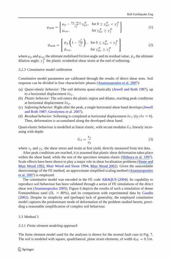
The finite element model used for the analyses is shown for the normal fault case in Fig. 7.The soil is modeled with square, quadrilateral, plane strain elements, of width dFE = 0.5 m.

123

Bull Earthquake Eng

Fig. 6 Method 2: Calibration ofconstitutive model—comparisonbetween laboratory direct sheartests on Fontainebleau sand(Gaudin 2002) and the results ofthe constitutive model

188.5 kPa

133.9 kPa

79.5 kPa

30.3 kPa

Analysis Test

v

160

120

80

40

00 1 2 3 4 5 6 7

x (mm)

(kP

a)

x

D

v

Fig. 7 Method 3 (Dynaflow) finite element diecretisation

Each element is defined with four nodes with two degrees of freedom at each node. Thefoundation, of width B, is modeled with quadrilateral infinitely stiff elements. It is connectedto the soil model with contact elements. The latter are used to impose inequality constraintsbetween the soil and the foundation; they are defined with three nodes and a penalty parameter.When the soil is in contact with the foundation, perfect friction is imposed; when separationbetween the foundation and the soil occurs no forces are transmitted from the soil to thefoundation.

The numerical problem is solved with an implicit explicit predictor (multi) correctorscheme; the non linear implicit solution algorithm used is a quasi Newton BFGS algorithmwith line search (Strang strategy) at each time step and a large displacement option. Theincremental displacement at the fault location is equal to 1 cm.

123

Bull Earthquake Eng

3.3.2 Soil constitutive Model

The constitutive model is the multi-yield constitutive model developed by Prevost (1989,1993). It is a kinematic hardening model, based on a relatively simple plasticity theory(Prevost 1985) and is applicable to both cohesive and cohesionless soils. The concept of a“field of work-hardening moduli” (Iwan 1967; Mróz 1967; Prevost 1977), is used by defininga collection f0, f1, . . ., fn of nested yield surfaces in the stress space. Von Mises type surfacesare employed for cohesive materials, and Drucker-Prager/Mohr-Coulomb type surfaces areemployed for frictional materials (sands).

The yield surfaces define regions of constant shear moduli in the stress space, and inthis manner the model discretises the smooth elastic-plastic stress–strain curve into n linearsegments. The outermost surface fn represents a failure surface. In addition, accounting forexperimental evidence from tests on frictional materials (e.g. Lade 1987), a non-associativeplastic flow rule is used for the dilatational component of the plastic potential.

Finally, the material hysteretic behavior and shear stress-induced anisotropic effects aresimulated by a kinematic rule. Upon contact, the yield surfaces are translated in the stressspace by the stress point, and the direction of translation is selected such that the yield surfacesdo not overlap, but remain tangent to each other at the stress point.

3.3.3 Constitutive model parameters

The required constitutive parameters of the multi-yield constitutive soil model are summari-sed as follows (Popescu and Prevost 1995):

a. Initial state parameters: mass density of the solid phase ρs , and for the case of poroussaturated media, porosity nw and permeability k.

b. Low strain elastic parameters: low strain moduli G0 and B0. The dependence of themoduli on the mean effective normal stress p′, is assumed to be of the following form:

G = G0

(p′

p′0

)n

B = B0

(p′

p′0

)n

(4)

and is accounted for, by introducing two more parameters: the power exponent n and thereference effective mean normal stress p′

0.c. Yield and failure parameters: these parameters describe the position ai , size Mi and

plastic modulus H ′i , corresponding to each yield surface fi , i = 0, 1, . . .n. For the case

of pressure sensitive materials, a modified hyperbolic expression proposed by Prevost(1989) and Griffiths and Prévost (1990) is used to simulate soil stress–strain relations. Thenecessary parameters are: (i) the initial gradient, given by the small strain shear modulusG0, and (ii) the stress (function of the friction angle at failure ϕ and the stress path) andstrain, εmax

dev , levels at failure. Hayashi et al. (1992) improved the modified hyperbolicmodel by introducing a new parameter—a—depending on the maximum grain size Dmax

and uniformity coefficient Cu . Finally, the coefficient of lateral stress K0 is necessary toevaluate the initial positions ai of the yield surfaces.

d. Dilation parameters: these are used to evaluate the volumetric part of the plastic potentialand consist of: (i) the dilation (or phase transformation) angle ϕ̄, and (ii) the dilationparameter Xpp , which is the scale parameter for the plastic dilation, and depends basicallyon relative density and sand type (fabric, grain size).

With the exception of the dilation parameter, all the required constitutive model parametersare traditional soil properties, and can be derived from the results of conventional laboratory

123

Bull Earthquake Eng

Table 1 Constitutive model parameters used in method 3

Number of yield surfaces 20 Power exponent n 0.5Shear modulus G at stress p1

(kPa)75,000 Bulk modulus at stress p1

(kPa)200,000

Unit mass ρ (t.m−3) 1.63 Cohesion 0Reference mean normal stress

p1 (kPa)100 Lateral stress coefficient (K0) 0.5

Dilation angle in compression( ◦)

31 Dilation angle in extension( ◦)

31

Ultimate friction angle incompression ( ◦)

41.8 Ultimate friction angle inextension ( ◦)

41.8

Dilation parameter Xpp 1.65Max shear strain in

compression0.08 Max shear strain in extension 0.08

Generation coefficient incompression αc

0.098 Generation coefficient inextension αe

0.095

Generation coefficient incompression αlc

0.66 Generation coefficient inextension αle

0.66

Generation coefficient incompression αuc

1.16 Generation coefficient inextension αue

1.16

(e.g. triaxial, simple shear) and in situ (e.g. cone penetration, standard penetration, wavevelocity) soil tests. The dilational parameter can be evaluated on the basis of results ofliquefaction strength analysis, when available; further details can be found in Popescu andPrevost (1995) and Popescu (1995).

Since in the present study the sand material is dry, the cohesionless material was modeledas a one-phase material. Therefore neither the soil porosity, nw , nor the permeability, k, areneeded.

For the shear stress–strain curve generation, given the maximum shear modulus G1, themaximum shear stress τmax and the maximum shear strain γmax, the following functionalrelationship has been chosen:

For y = τ /τmax and x = γ /γr , with γr = τmax/G1, then:

y = exp (−ax) f (x, xl)+ (1 − exp (−ax)) f (x, xu)

where:

f (x, xi ) = [(2x/xi + 1)xi − 1

]/[(2x/xi + 1)xi + 1

] (5)

where a, xl and xu are material parameters. For further details, the reader is referred toHayashi et al. (1992).

The constitutive model is implemented in the computer code DYNAFLOW (Prevost 1981)that has been used for the numerical analyses.

3.3.4 Calibration of model constitutive parameters

To calibrate the values of the constitutive parameters, numerical triaxial tests were simulatedwith DYNAFLOW at three different confining pressures (30, 60, 90 kPa) and compared withthe results of available physical tests conducted on the same material at the same confiningpressures. The parameters are defined based on the shear stress versus axial strain curveand volumetric strain versus axial strain curve. Figure 8 illustrates the comparisons betweennumerical simulations and physical tests in terms of volumetric strain and shear stress versus

123

Bull Earthquake Eng

Fig. 8 Method 3: Calibration of constitutive model parameters; triaxial tests at 60 kPa

axial strain for the test conducted with a confining pressure of 60 kPa. The parameters finallyretained for a complete definition of the constitutive model used for the numerical finiteelement analyses are listed in Table 1.

4 Comparison between numerical analysis approaches

To evaluate the effectiveness of the developed numerical analysis approaches, we compareexperimental data of centrifuge model tests with analytical predictions. First, the comparisonis conducted for the free-field part of the problem, to highlight the capability of the differentmodels in predicting the rupture path, the location of fault outcropping (defined as the pointwhere the steepest gradient is observed), and the deformation of the ground surface. Twocentrifuge tests are utilised for this purpose: (a) Test 12, normal faulting at 60 ◦; and (b) Test28, reverse faulting at 60 ◦. Since the free-field cases had not been analysed with the moreelaborate Method 3, the comparison is restricted to the first two methods (1 and 2).

Then, two other centrifuge tests with shallow foundations are compared to shed morelight in the robustness of the FE approaches with respect to Fault Rupture–Soil–Foundation–

123

Bull Earthquake Eng

Table 2 Summary of main attributes of the centrifuge model tests

Test Faulting B (m) q (kPa) s (m) g-Levela Dr (%) H (m) L (m) W (m) hmax (m)

12 Normal Free—field 115 60.2 24.7 75.7 23.5 3.1528 Reverse Free—field 115 60.8 15.1 75.7 23.5 2.5914 Normal 10 91 2.9 115 62.5 24.6 75.7 23.5 2.4929 Reverse 10 91 9.2 115 64.1 15.1 75.7 23.5 3.30

a Centrifugal acceleration

Fig. 9 Test 12—Free-field faultrupture propagation throughDr = 60% Fontainebleau sand(α = 60 ◦): Comparison ofnumerical with experimentalvertical displacement of thesurface for bedrock dislocationh = 3.0 m (Method 1) and 2.5 m(Method 2) [all displacements aregiven in prototype scale]

-3,5

-3

-2,5

-2

-1,5

-1

-0,5

0

-30 -25 -20 -15 -10 -5 10

x (m)

y (m

)

Test: h = 2.94 m

Method 1: h = 3 m

Test: h = 2.47 m

Method 2: h = 2.5 m

0 5

Structure Interaction (FR-SFSI): (i) Test 14, normal faulting at 60 ◦; and (ii) Test 29, reversefaulting at 60 ◦. In this case, the comparison is conducted for all of the developed numericalanalysis approaches.

The main attributes of the four centrifuge model tests used for the comparisons are syn-opsised in Table 2, while more details can be found in Bransby et al. (2008a, b).

4.1 Free-field fault rupture propagation

4.1.1 Test12—normal 60 ◦

This test was conducted at 115 g on medium-loose (Dr = 60%) Fontainebleau sand, simu-lating normal fault rupture propagation through an H = 25 m soil deposit. The comparisonbetween analytical predictions and experimental data is depicted in Fig. 9 in terms of verticaldisplacement�y at the ground surface. All displacements are given in prototype scale. Whilethe analytical prediction of Method 1 is compared with test data for h = 3.0 m, in the caseof Method 2 the comparison is conducted at slightly lower imposed bedrock displacement:h = 2.5 m. This is due to the fact that the numerical analysis with Method 2 was conductedwithout knowing the test results, and at that time it had been agreed to set the maximumdisplacement equal to hmax = 2.5 m. However, when test results were publicised, the actuallyattained maximum displacement was larger, something that was taken into account in theanalyses with Method 1.

As illustrated in Fig. 9, Method 2 predicts almost correctly the location of fault out-cropping, at about—10 m from the “epicenter”, with discrepancies limited to 1 or 2 m. Thedeformation can be seen to be slightly more localised in the centrifuge test, but the comparisonbetween analytical and experimental shear zone thickness is quite satisfactory. The verticaldisplacement profile predicted by Method 1 is also qualitatively acceptable. However, the

123

Bull Earthquake Eng

Method 2

Centrifuge Model Test

R1

S1

Method 1

(a)

(b)

(c)

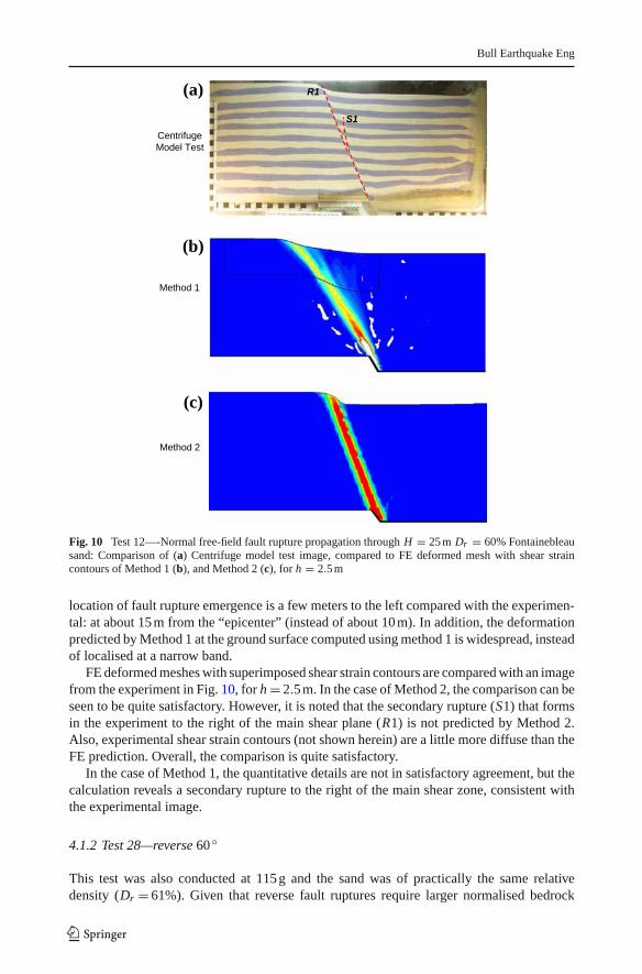
Fig. 10 Test 12—-Normal free-field fault rupture propagation through H = 25 m Dr = 60% Fontainebleausand: Comparison of (a) Centrifuge model test image, compared to FE deformed mesh with shear straincontours of Method 1 (b), and Method 2 (c), for h = 2.5 m

location of fault rupture emergence is a few meters to the left compared with the experimen-tal: at about 15 m from the “epicenter” (instead of about 10 m). In addition, the deformationpredicted by Method 1 at the ground surface computed using method 1 is widespread, insteadof localised at a narrow band.

FE deformed meshes with superimposed shear strain contours are compared with an imagefrom the experiment in Fig. 10, for h = 2.5 m. In the case of Method 2, the comparison can beseen to be quite satisfactory. However, it is noted that the secondary rupture (S1) that formsin the experiment to the right of the main shear plane (R1) is not predicted by Method 2.Also, experimental shear strain contours (not shown herein) are a little more diffuse than theFE prediction. Overall, the comparison is quite satisfactory.

In the case of Method 1, the quantitative details are not in satisfactory agreement, but thecalculation reveals a secondary rupture to the right of the main shear zone, consistent withthe experimental image.

4.1.2 Test 28—reverse 60 ◦

This test was also conducted at 115 g and the sand was of practically the same relativedensity (Dr = 61%). Given that reverse fault ruptures require larger normalised bedrock

123

Bull Earthquake Eng

Fig. 11 Test 28—Reversefree-field fault rupturepropagation through H = 15 mDr = 60% Fontainebleau sand:Comparison of numerical withexperimental verticaldisplacement of the surface forbedrock dislocation h = 2.0 m(all displacements are given inprototype scale)

-0,5

0

0,5

1

1,5

2

2,5

-30 -25 -20 -15 -10 -5

x (m)

y (m

)

Test

Method 1

Method 2

0 5

displacement h/H to propagate all the way to the surface (e.g. Cole and Lade 1984; Ladeet al. 1984; Anastasopoulos et al. 2007; Bransby et al. 2008b), the soil depth was set atH = 15 m. This way, a larger h/H could be achieved with the same actuator.

Figure 11 compares the vertical displacement �y at the ground surface predicted bythe numerical analysis to experimental data, for h = 2.0 m. This time, both models predictcorrectly the location of fault outcropping (defined as the point where the steepest gradientis observed). In particular, Method 1 achieves a slightly better prediction of the outcroppinglocation: −10 m from the epicentre (i.e., a difference of 1 m only, to the other direction).Method 2 predicts the fault outbreak at about −7 m from the “epicenter”, as opposed to about−9 m of the centrifuge model test (i.e., a discrepancy of about 2 m).

Figure 12 compares FE deformed meshes with superimposed shear strain contours withan image from the experiment, for h = 2.5 m. In the case of Method 2, the numerical analysisseems to predict a distinct fault scarp, with most of the deformation localised within it. Incontrast, the localisation in the experiment is clearly more intense, but the fault scarp atthe surface is much less pronounced: the deformation is widespread over a larger area. Theanalysis with Method 1 is successful in terms of the outcropping location. However, instead ofa single rupture, it predicts the development of two main ruptures (R1 and R2), accompaniedby a third shear plane in between. Although such soil response has also been demonstrated byother researchers (e.g. Loukidis and Bouckovalas 2001), in this case the predicted multiplerupture planes are not consistent with experimental results.

4.2 Interaction with strip footings

Having validated the effectiveness of the developed numerical analysis methodologies insimulating fault rupture propagation in the free-field, we proceed to the comparisons ofexperiments with strip foundations: one for normal (Test 14), and one for reverse (Test 29)faulting. This time, the comparison is extended to all three methods.

4.2.1 Test 14—normal 60 ◦

This test is practically the same with the free-field Test 12, with the only difference beingthe presence of a B = 10 m strip foundation subjected to a bearing pressure q = 90 kPa. Thefoundation is positioned so that the free-field fault rupture would emerge at distance s = 2.9 mfrom the left edge of the foundation.

123

Bull Earthquake Eng

Centrifuge Model Test

(a)

Method 2

(c)

Method 1

(b)R1

R2

Fig. 12 Test 28—Reverse free-field fault rupture propagation through H = 15 m Dr = 60% Fontainebleausand: Comparison of (a) Centrifuge model test image, compared to FE deformed mesh with shear straincontours of Method 1 (b), and Method 2 (c), for h = 2.5 m

Fig. 13 Test 14—Interaction ofnormal α = 60 ◦ fault rupture,through H = 25 m sand deposit,with rigid B = 10 m foundationsubjected to surcharge loadq = 90 kPa, positioned atdistance s = 2.9 m: Verticaldisplacement profile at thesurface, h = 2.5 m (alldisplacements are given inprototype scale)

-3

-2,5

-2

-1,5

-1

-0,5

0

-30 -25 -20 -15 -10 -5 0 5 10

x (m)

y (m

)

TestMethod 1Method 2Method 3

Figure 13 compares experimental results with numerical predictions in terms of verticaldisplacement �y at the ground surface for bedrock displacement h = 2.5 m. The agreementis satisfactory for all three modelling methodologies. All FE analyses predict correctly thediversion of the fault rupture to the left of the foundation. While in Test 12 (free-field) therupture outcropped at d =−10 m from the “epicenter”, in the presence of the foundation it isdiverted to emerge at d =−13 m. Despite this diversion, the foundation is subjected to rigidbody rotation �θ .

Figure 14 shows that the three numerical methodologies yield different results in terms offoundation rotation �θ with respect to h. The numerical prediction obtained with Method 1leads to an underestimation of �θ (probably due to the ψ = 0 ◦ assumption): for h = 2.5 mMethod 1 predicts �θ = 0.5 ◦ (instead of 2.1 ◦ measured in the experiment). In contrast,

123

Bull Earthquake Eng

Fig. 14 Test 14—Interaction ofnormal α = 60 ◦ fault rupture,through H = 25 m sand deposit,with rigid B = 10 m foundationsubjected to surcharge loadq = 90 kPa, positioned atdistance s = 2.9 m: Foundationrotation �θ versus bedrock faultoffset h

0

1

2

3

4

5

0 0,5 1 1,5 2 2,5

h (m) (

deg

)

TestMethod 1Method 2Method 3

with the exception of the region of small imposed displacement (h< 1 m), the predictionof Method 2 is in good agreement with the experiment: at h = 2.5 m, the analysis predicts�θ = 1.9 ◦ (compared with 2.1 ◦ in the test). Finally, the prediction of Method 3 indicates analmost linear increase of�θ with imposed bedrock displacement h, leading to overestimationof the footing rotation at large h (probably due to the fact that the model does not take accountof strain softening). More specifically, for h = 2.5 m, Method 3 predicts �θ = 4.8 ◦ insteadof the measured 2.1 ◦, but gives good predictions at small fault offsets (h ≤ 0.5 m).

A centrifuge model test image is compared with FE computed deformed meshes withsuperimposed vertical displacement contours in Fig. 15 for h = 2.5 m. All three numericalapproaches predict correctly the diversion of the main fault rupture (R1’) to the left ofthe foundation (towards the footwall). As already discussed, the main difference lies in thefoundation rotation �θ . In the experiment, a secondary steep rupture zone, S1’ (practicallythe same as S1 of Test 12), develops and propagates half the way to the surface before R1’is formed (see also Bransby et al. 2008a).

4.2.2 Test 29—reverse 60 ◦

Test 29 is practically the same as free-field Test 28, with the only difference being the presenceof a B = 10 m strip foundation subjected to q = 90 kPa, positioned at s = 9.2 m.

Figure 16 compares experimental data with analytical predictions in terms of �y at thesoil surface for h = 2.5 m. This time, the differences between the three numerical approachesare negligible, with all three vertical displacement profiles exhibiting similar behaviour, andin general agreement with the experimental observations. All three numerical approachesindicate some soil heave on the left side of the foundation, which may be caused by thecompression induced by foundation rotation. However, in the case of Methods 1 and 2,the heave is limited to a smaller area very close to the foundation edge. This behaviouris attributable to the inherent differences of the adopted constitutive models. All three FEmodels predict correctly the diversion of the rupture path to the right of the foundation, whilethe differences in terms of foundation rotation�θ are much smaller than for the normal faultcase.

As illustrated in Fig. 17, the numerical prediction of Method 1 generally overestimates�θ : for h = 2.5 m Method 1 predicts �θ = 2.4 ◦. The results of Method 2 are different,exhibiting a softening-like behaviour. As a result,�θ is initially (h ≤ 2 m) overestimated, butin the end (h = 2.5 m) the analysis yields slightly lower�θ compared to the experiment: 1.4 ◦instead of the measured 1.6 ◦. Method 3 indicates an increase of�θ with respect to h with anincreasing rate. Thus, while at the beginning it underestimates the rotation of the foundation,

123

Bull Earthquake Eng

(a)

(b)

(c)

(d)

Fig. 15 Test 14—Interaction of normal α = 60 ◦ fault rupture, through H = 25 m sand deposit, with rigidB = 10 m foundation subjected to surcharge load q = 90 kPa, positioned at distance s = 2.9 m: Centrifugemodel test image (a), compared to FE deformed mesh with shear strain contours of Method 1 (b), Method 2(c), and Method 3 (d), for h = 2.5 m

at larger imposed displacement h it tends to slightly overestimate it: for h = 2.5 m, it predicts�θ = 2.0 ◦ instead of the measured 1.6 ◦.

Figure 18 compares a centrifuge model test image with the computed deformed FE mes-hes with superimposed vertical displacement contours (for h = 2.5 m). The shear planespredicted by Methods 1 and 2 are quite localised, with plastic deformation within a narrowband, in good agreement with the centrifuge model test. The Method 3-predicted deformedmesh is characterised by a wider shear zone. The Method 1 numerical result can be seen to bein good agreement with the centrifuge test in terms of the soil overlapping at the right edge ofthe footing. However, in the centrifuge test a secondary localisation is also formed. It initiatesfrom the top-right (footwall-side) edge of the foundation and propagates downwards. This

123

Bull Earthquake Eng

Fig. 16 Test 29—Interaction ofreverse α = 60 ◦ fault rupture,through H = 15 m sand deposit,with rigid B = 10 m foundationsubjected to surcharge loadq = 90 kPa, positioned atdistance s = 9.2 m: Verticaldisplacement profile at thesurface, h = 2.5 m (alldisplacements are given inprototype scale)

-0,5

0

0,5

1

1,5

2

2,5

3

-30 -25 -20 -15 -10 -5 0 5 10

x (m)

y (m

)

TestMethod 1

Method 2Method 3

Fig. 17 Test 29—Interaction ofreverse α = 60 ◦ fault rupture,through H = 15 m sand deposit,with rigid B = 10 m foundationsubjected to surcharge loadq = 90 kPa, positioned atdistance s = 9.2 m: Foundationrotation �θ versus bedrock faultoffset h

0

0,5

1

1,5

2

2,5

0 0,5 1 1,5 2 2,5

h (m)

(d

eg)

TestMethod 1Method 2Method 3

takes place at the later stages of the experiment, when the top side of the foundation gainscontact with the upwards displacing soil. The numerical analyses cannot possibly capture thisfeature, since no contact elements have been placed between the side edges of the foundationand the soil surface.

5 Parametric analysis

5.1 Methodology

Having validated the three FE analysis methodologies developed within the QUAKER rese-arch project, we apply Method 2 to conduct a short parametric study of typical residentialstructures subjected to normal fault dislocation.

The main factors influencing FR-SFSI are (Anastasopoulos and Gazetas 2007b):

(a) The type and continuity of the foundation system (isolated footings, raft, piles).(b) The flexural and axial rigidity of the foundation system (e.g. thickness of mat foundation).(c) The surcharge load of the superstructure.(d) The stiffness of the superstructure (cross section of structural members, grid spacing).(e) The soil stiffness and strength.(f) The position of the structure relative to the fault rupture (distance s).

All of the above factors are examined herein, with the exception of the type of foundationsystem: given that the continuity of the foundation system has already been shown to be

123

Bull Earthquake Eng

Method 3

Method 2

Method 1

Foundation

Centrifuge Model Test

Foundation

(a)

(b)

(c)

(d)

Fig. 18 Test 29—Interaction of reverse α = 60 ◦ fault rupture, through H = 15 m sand deposit, with rigidB = 10 m foundation subjected to surcharge load q = 90 kPa, positioned at distance s = 9.2 m: Centrifugemodel test image (a), compared to FE deformed mesh with shear strain contours of Method 1 (b), Method 2(c), and Method 3 (d), for h = 2.5 m

crucial for the response of a structure (Anastasopoulos and Gazetas 2007b; Faccioli et al.2008), we will focus on buildings resting on mat foundations (slab or box-type).

Without underestimating the general importance of the details of a superstructure, wetreat all of the analysed structures as “equivalent” in this respect, changing only the numberof storeys. This way it is easier to develop insights on the influence of the type and stiff-ness of their foundation, and on the effect of the surcharge load on FR-SFSI. Therefore, atypical column grid of 5 × 5 m is utilised, in combination with a structure width B = 20 m.Columns and beams are of 50 cm square cross-section, taking into account the contributionof walls and slabs. Such a hypothesis can be considered as realistic for 2- to 5-story buildings(Anastasopoulos and Gazetas 2007b).

To explore the role of foundation stiffness EI, the equivalent thickness of the slab foun-dation is varied from t = 0.2 to 0.5 m, and 1.3 m, yielding E I = 2.0 × 105, 3.1 × 106, and5.5 × 107 kNm2. It is noted that the stiffness of the foundation is coupled to its dead load,which is added to the overall equivalent surcharge load of the superstructure, q. The distanceof the outcropping fault to the left edge of the structure is also varied: s = 4, 10 m, and 16 m

123

Bull Earthquake Eng

B = 20 m

t = 0.2 m

s = 4 m

s = 10 m

s = 16 m

0.5 m1.3 m

B = 20 m

t = 0.2 m

s = 4 m

s = 10 m

s = 16 m

0.5 m1.3 m

(a)

(b)

Fig. 19 Idealised structures of the parametric study: (a) 2-storey, B = 20 m building, and (b) 5-storey,B = 20 m building

(s/B = 0.2, 0.5, and 0.8, respectively). The 18 idealised structures are illustrated in Fig. 19;their properties are summarised in Table 3.

Given the multitude of structure–foundation–position combinations to be analysed, a dipangle a = 60 ◦ has been selected for all of the analyses, considered typical for normal faults.To investigate the role of soil compliance, our idealised structures are analysed in conjunctionwith two idealised types of sand (Anastasopoulos et al. 2007):

• Dense Sand: ϕp = 45 ◦, ϕres = 30 ◦, ψp = 18 ◦, γy = 0.015, and γ Pf = 0.0516

• Loose Sand: ϕp = 32 ◦, ϕres = 30 ◦, ψp = 3 ◦, γy = 0.030, and γ Pf = 0.0616

The idealised dense sand is stiffer and reaches failure at relatively low strains (γy = 1.5%).Hence, as demonstrated in Anastasopoulos et al. (2007), it exhibits “brittle” behaviour allo-wing for the rupture to outcrop at relatively small normalised bedrock displacement h/H . On

123

Bull Earthquake Eng

Table 3 Properties of the idealised structures of the parametric fault-foundation interaction study

Normaliseddistance s/B

Idealisedsand type

Number ofstories (#)

Raft thickness(m)

Foundationstiffness EI(kNm2)

Equivalentdead loadq (kN/m)

0.2 Dense 2 0.2 2.0 × 105 25.00.5 3.1 × 106 32.51.3 5.5 × 107 52.5

5 0.2 2.0 × 105 55.00.5 3.1 × 106 62.51.3 5.5 × 107 82.5

Loose 2 0.2 2.0 × 105 25.00.5 3.1 × 106 32.51.3 5.5 × 107 52.5

5 0.2 2.0 × 105 55.00.5 3.1 × 106 62.51.3 5.5 × 107 82.5

0.5 Dense 2 0.2 2.0 × 105 25.00.5 3.1 × 106 32.51.3 5.5 × 107 52.5

5 0.2 2.0 × 105 55.00.5 3.1 × 106 62.51.3 5.5 × 107 82.5

Loose 2 0.2 2.0 × 105 25.00.5 3.1 × 106 32.51.3 5.5 × 107 52.5

5 0.2 2.0 × 105 55.00.5 3.1 × 106 62.51.3 5.5 × 107 82.5

0.8 Dense 2 0.2 2.0 × 105 25.00.5 3.1 × 106 32.51.3 5.5 × 107 52.5

5 0.2 2.0 × 105 55.00.5 3.1 × 106 62.51.3 5.5 × 107 82.5

Loose 2 0.2 2.0 × 105 25.00.5 3.1 × 106 32.51.3 5.5 × 107 52.5

5 0.2 2.0 × 105 55.00.5 3.1 × 106 62.51.3 5.5 × 107 82.5

the other hand, the idealised loose sand is more compliant and reaches failure at higher strainlevels (γy = 3%). It is therefore expected to exhibit more “ductile” behaviour, allowing forthe rupture to delay its emergence.

5.2 Summary of results

The discussion of all of the results of the parametric study is clearly beyond the scope of thispaper. Hence, a summary of the results is presented in the following sections, focusing onthe effect of: (i) the distance s, (ii) the equivalent surcharge load q, and (iii) soil compliance

123

Bull Earthquake Eng

(dense versus loose sand). The effect of foundation stiffness has been investigated in moredetail in Anastasopoulos et al. (2008), and shall not be repeated here.

The results are discussed in terms of deformed mesh with superimposed plastic shearstrains, the soil vertical displacement profile �y, and the contact pressure p along the foun-dation. In all cases the results are compared with the free-field to deduce the effect of FR-SFSI.The contact pressure is compared with its initial distribution (h = 0, before application of thedislocation) to reveal which parts of the structure are loosing contact with the bearing soil:foundation uplifting. The left part of the building that uplifts is denoted as uL , the right u R ,and u if the uplifting takes place near the centre. Accordingly, the parts of the foundation thatmaintain contact with the soil are denoted as bL and bR , depending if it is at the left or rightside of the building, and b if it is at the centre. The differential settlement of the foundation Dyis also reported to provide an estimate of the relative distress of each structure, mainly in termsof functionality. Finally, the maximum amplitude of bending moment of the superstructure,MS,max, and the foundation, MF,max, is also reported as a measure of structural distress.

5.2.1 Illustration of the effect of distance s

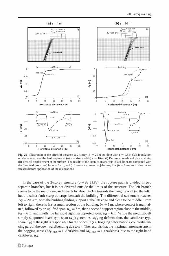
The effect of the position of the building relative to the unperturbed (free-field) fault rupture, asexpressed through distance s, is illustrated in Fig. 20. We compare the response of the idealised2-storey building resting on dense sand and founded through a t = 0.5 m raft foundation,positioned at s = 4 m and 16 m.

In the first case, the building is mainly resting on the footwall, not causing any significantdiversion of the rupture path. The differential settlement does not exceed �y = 19 cm, withthe bending moment of foundation and superstructure reaching MF,max = 1, 547 kNm andMS,max = 735 kNm, respectively. The stressing of the structure is mainly due to its detachmentfrom the bearing soil: the building loses contact at both sides, uL = 6 m, u R = 3 m; with onlyits central part maintaining contact at a width b = 11 m. The two unsupported spans (u R anduL ) essentially act as cantilevers on “elastic” supports, generating hogging deformation ofthe structure.

By moving the dislocation to s = 16 m, the interaction effects are altered significantly.The rupture is now divided in two separate branches. The right one diverts slightly towardsthe footwall by about 2 m, while the left is equally diverted towards the hanging wall (byabout 3 m). A fault scarp is formed near the right edge of the building. As a consequence, themiddle part of the building looses contact with the bearing soil, u = 11 m, while the left andright part of it are the ones that bear the load of the structure, bL = 2 m and bR = 7 m. While,the differential displacement reaches �y = 159 cm, the bending moments are not increasedaccordingly: MF,max = −1, 354 kNm and MS,max =−995 kNm. The structure is supported atits two edges (bL and bR), with its central detached span (u) acting as a “simply supported”beam on “elastic” supports. Now, the bending of the whole structure is to the oppositedirection, i.e. sagging deformation (this is the reason for the negative sign in MF,max andMS,max).

5.2.2 Illustration of the effect of surcharge load q

To illustrate the effect of the equivalent surcharge load q, we compare a 2-storey to a 5-storeybuilding (Fig. 21). Both buildings are positioned at s = 10 m, resting on dense sand, andfounded through a t = 0.5 m slab foundation.

123

Bull Earthquake Eng

-2

-1.5

-1

-0.5

0

0 5 10 15 20 25 30

-200

-150

-100

-50

0

0 5 10 15 20 25 30-200

-150

-100

-50

0

0 5 10 15 20 25 30

-2

-1.5

-1

-0.5

0

0 5 10 15 20 25 30

(i)

Free Field

(ii)

(iii)

y = 19 cm

(a) s = 4 m

Horizontal distance x (m)

p (

kPa)

Horizontal distance x (m)

y (m

)

building

building

h = 2 m

h = 0

free-fieldInteraction

MS,max = 735 kNmMF,max = 1547 kNm

(i)

Free Field

y = 159 cm

(b) s = 16 m

Horizontal distance x (m)

p (

kPa)

Horizontal distance x (m)

y (m

)

(ii)

(iii)

building

building

h = 2 m

h = 0

free-field

Interaction

MS,max = –995 kNmMF,max = –1354 kNm

uL = 6 m uR = 3 m

b = 11 m

bR = 7 mbL = 2 m

u = 11 m

Fig. 20 Illustration of the effect of distance s: 2-storey, B = 20 m building with t = 0.5 m slab foundationon dense sand, and the fault rupture at (a) s = 4 m, and (b) s = 16 m; (i) Deformed mesh and plastic strain,(ii) Vertical displacement at the surface [The results of the interaction analysis (black line) are compared withthe free-field (grey line) for h = 2 m.], and (iii) contact stresses σv, [the grey line (h = 0) refers to the contactstresses before application of the dislocation]

In the case of the 2-storey structure (q = 32.5 kPa), the rupture path is divided in twoseparate branches, but it is not diverted outside the limits of the structure. The left branchseems to be the major one, and diverts by about 2–3 m towards the hanging wall (to the left),but a distinct fault scarp outcrops beneath the building. The differential settlement reaches�y = 206 cm, with the building finding support at the left edge and close to the middle. Fromleft to right, there is first a small section of the building, bL = 1 m, where contact is maintai-ned, followed by an uplifted span, uL = 7 m, then a second support region close to the middle,bR = 6 m, and finally the far most right unsupported span, u R = 6 m. While the medium-leftsimply supported beam-type span (uL ) generates sagging deformation, the cantilever-typespan (u R) at the right is responsible for the opposite (i.e. hogging deformation), counterbalan-cing part of the downward bending due to uL . The result is that the maximum moments are inthe hogging sense (MF,max = 1, 870 kNm and MS,max = 1, 094 kNm), due to the right-handcantilever, u R .

123

Bull Earthquake Eng

-200

-150

-100

-50

0

0 5 10 15 20 25 30

-2

-1.5

-1

-0.5

0

0 5 10 15 20 25 30

-200

-150

-100

-50

0

0 5 10 15 20 25 30

-2

-1.5

-1

-0.5

0

0 5 10 15 20 25 30

y = 230 cm

(i)

Free Field

(ii)

(iii)

(a) 2-stories : q = 32.5 kPa

(i)

(b) 5-stories : q = 62.5 kPa

Horizontal distance x (m) Horizontal distance x (m)

p (

kPa)

p (

kPa)

Horizontal distance x (m) Horizontal distance x (m)

y (m

)

y (m

)

(ii)

(iii)

building building

building building

h = 2 m

h = 0

h = 0

free-field Interaction

free-field

Interaction

MS,max = 1094 kNmMF,max = 1870 kNm

MS,max = 885 kNmMF,max = –2088 kNm

Free Field

y = 206 cm

uL = 7 m

bL = 1 m

bR = 6 m

uR = 6 mh = 2 m

uL = 5 m

bL = 1 m

bR = 10 m

uR = 4 m

Fig. 21 Illustration of the effect of the equivalent surcharge load q: B = 20 m building, with t = 0.5 mslab foundation on dense sand, fault rupture at s = 10 m; (a) 2-storeys (q = 32.5 kPa), and (b) 5-storeys(q = 62.5 kPa); (i) Deformed mesh and plastic strain, (ii) Vertical displacement at the surface [The resultsof the interaction analysis (black line) are compared with the free-field (grey line) for h = 2 m.], and(iii) contact stresses σv, [the grey line (h = 0) refers to the contact stresses before application of thedislocation]

The response of the 5-storey structure (q = 62.5 kPa) is qualitatively the same, but due tothe increased surcharge load the diversion of the rupture is more intense. The rupture pathis again divided in two separate branches, with the left one diverting by about 3 m towardsthe hanging wall, and the right one about 6 m to the right (towards the footwall). As a result,the differential displacement is reduced to �y = 188 cm. Besides from the larger diversionof the right branch of the rupture, the increase of q also leads to a decrease of the detachedregions of the building: bL = 1, uL = 5, bR = 10, and u R = 4 m. The result is a reduction ofMS,max to 885 kNm, despite the fact that q is practically doubled. Notice also that MF,max

is now negative (sagging) and only marginally larger (−2, 088 kNm). This indicates thatthe decrease of the simply supported beam-type span uL (from 7 to 5 m) overshadows theeffect of the decrease of the cantilever-type span u R (from 6 to 4 m) so that there is a net(uL -induced) sagging deformation.

123

Bull Earthquake Eng

-200

-150

-100

-50

0

0 5 10 15 20 25 30

-2

-1.5

-1

-0.5

0

0 5 10 15 20 25 30

-2

-1.5

-1

-0.5

0

0 5 10 15 20 25 30

-200

-150

-100

-50

0

0 5 10 15 20 25 30

Free Field

y = 68 cm

(i)

(b) Loose sand

Horizontal distance x (m)

p (

kPa)

Horizontal distance x (m)

y (m

)

(ii)

(iii)

building

building

h = 2 m

h = 0

free-field

Interaction

MS,max = –503 kNmMF,max = –912 kNm

(i)

Free Field

y = 159 cm

(a) Dense sand

Horizontal distance x (m)

p (

kPa)

Horizontal distance x (m)

y (m

)

(ii)

(iii)

building

building

h = 2 m

h = 0

free-field

Interaction

MS,max = –995 kNmMF,max = –1354 kNm

bR = 7 mbL = 2 m

u = 11 m

Fig. 22 Illustration of the effect of soil compliance: 2-storey, B = 20 m building, fault rupture at s = 16 m,resting on t = 0.5 m raft foundation; (a) Dense sand, and (b) Loose sand; (i) Deformed mesh and plastic strain,(ii) Vertical displacement at the surface [The results of the interaction analysis (black line) are compared withthe free-field (grey line) for h = 2 m.], and (iii) contact stresses σv, [the grey line (h = 0) refers to the contactstresses before application of the dislocation]

5.2.3 Illustration of the effect of soil compliance

The effect of soil compliance is illustrated in Fig. 22. We compare the response of the idealised2-storey building on t = 0.5 m slab foundation, and at s = 16 m, resting on the idealised denseand loose sand.

Given that the first case has already been discussed, we mainly focus on the differencesbetween the two types of sand. First of all, while in dense sand the fault rupture is dividedin two separate branches, with the left of them outcropping beneath the structure, in thecase of loose sand the rupture is clearly diverted to the right edge. As a result, the buildingmaintains full contact, b = 20 m, and the differential settlement is decreased substantially to�y = 68 cm (compared to 159 cm). Equally significant is the decrease of the stressing of thestructure: MF,max = − 912 kNm and MS,max = − 503 kNm. It is noted, however, that even

123

Bull Earthquake Eng

b/B

u/B

u/B

b/B

b/B

; u

/B

q (kPa)0 20 40 60 80 100

1.0

0.8

0.6

0.4

0.2

0

b/B

u/B

u/B

q (kPa)0 20 40 60 80 100

b/B

u/B

b/B

b/B

; u

/B

q (kPa)0 20 40 60 80 100

1.0

0.8

0.6

0.4

0.2

0

b/Bu/B

q (kPa)0 20 40 60 80 100

DENSE

b/B

u/B

u/B

b/B

; u

/B

q (kPa)0 20 40 60 80 100

1.0

0.8

0.6

0.4

0.2

0

b/B

u/B

q (kPa)0 20 40 60 80 100

LOOSE

(a) s/B = 0.2

(b) s/B = 0.5

(c) s/B = 0.8

Cantilever-type span

Simply supported beam–type span

Cantilever-type span

Cantilever-type span

Cantilever-type span

Cantilever-type span

Simply supported beam–type span

Fig. 23 Summary of analysis results illustrating the normalised (to the width B) uplifted, u/B, and effective,b/B, regions of the foundation with respect to the equivalent surcharge load q, and soil compliance for:(a) s/B = 0.2, (b) s/B = 0.5, and (c) s/B = 0.8. Results are plotted for h = 2 m

without any detachment taking place, the structure is subjected to some noticeable stressing.The latter is attributable to the deformation of the soil mass supporting the building.

5.3 Synopsis

The results of the parametric study are summarised in Figs. 23 and 24. Emphasis is placedon the effect of the surcharge load q, soil compliance (dense versus loose sand), and thedistance s.

Figure 23 illustrates the detached (unsupported), u, and effective, b, regions of the foun-dation with respect to the equivalent surcharge load q, and soil compliance for the threeinvestigated locations relative to the free-field fault rupture (s/B = 0.2, 0.5, and 0.8). Both uand b are normalised to the width of the foundation B.

123

Bull Earthquake Eng

Fig. 24 Summary of analysisresults illustrating the rotation�θ of the structure with respectto the equivalent surcharge loadq, and soil compliance for:(a) s/B = 0.2, (b) s/B = 0.5, and(c) s/B = 0.8. Results are plottedfor h = 2 m

0

2

4

6

8

10

12

0

2

4

6

8

10

12

0

2

4

6

8

10

12

0 20 40 60 80 100

(a) s/B= 0.2

(b) s/B= 0.5

(c) s/B= 0.8

DenseLoose

DenseLoose

DenseLoose

(%)

(%)

(%)

q (kPa)

In dense sand, for s/B = 0.2 the increase of q leads to an increase of the effective foundationwidth b/B from 0.6 to 0.75, reducing the maximum (unsupported) cantilever-type span fromu/B = 0.25 to 0.20. Similarly, for s/B = 0.5 the increase of q leads to the decrease of thecantilever-type u/B from 0.25 to 0.20, and of the simply supported beam-type u/B from0.30 to 0.25. In stark contrast, in the case of s/B = 0.8 the increase of q does not seem toplay a significant role. In loose sand, for s/B = 0.2 the increase of q limits the maximumcantilever-type u/B to 0.10 instead of 0.15. For s/B = 0.5 and 0.8, the increase of q leads tofull contact: b/B → 1.0.

Figure 24 depicts the rotation of the foundation �θ , with respect to q, s/B, and soilcompliance, for h = 2 m. When the rupture outcrops close to the left edge of the foundation,s/B = 0.2, the increase of q leads to significant increase of �θ in the case of loose sand,but practically no increase at all in dense sand. Soil compliance can clearly be seen to actunfavorably with respect to foundation rotation: �θ is larger in loose sand. In contrast, for

123

Bull Earthquake Eng

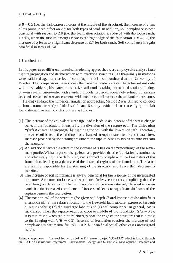
s/B = 0.5 (i.e. the dislocation outcrops at the middle of the structure), the increase of q hasa less pronounced effect on �θ for both types of sand. In addition, soil compliance is nowbeneficial with respect to �θ (i.e. the foundation rotation is reduced with the loose sand).Finally, when the rupture emerges close to the right edge of the foundation, s/B = 0.8, theincrease of q leads to a significant decrease of �θ for both sands. Soil compliance is againbeneficial in terms of �θ .

6 Conclusions

In this paper three different numerical modelling approaches were employed to analyse faultrupture propagation and its interaction with overlying structures. The three analysis methodswere validated against a series of centrifuge model tests conducted at the University ofDundee. The comparisons have shown that reliable predictions can be achieved not onlywith reasonably sophisticated constitutive soil models taking account of strain softening,but—in several cases—also with standard models, provided adequately refined FE meshesare used, as well as interface elements with tension cut-off between the soil and the structure.

Having validated the numerical simulation approaches, Method 2 was utilised to conducta short parametric study of idealised 2- and 5-storey residential structures lying on slabfoundations. The main conclusions are as follows:

[1] The increase of the equivalent surcharge load q leads to an increase of the stress changebeneath the foundation, intensifying the diversion of the rupture path. The dislocation“finds it easier” to propagate by rupturing the soil with the lowest strength. Therefore,since the soil beneath the building is of enhanced strength, thanks to the additional stressincrease provided by the bearing pressure q, the rupture bends to avoid this zone beneaththe structure.

[2] An additional favorable effect of the increase of q lies on the “smoothing” of the settle-ment profile. With a larger surcharge load, and provided that the foundation is continuousand adequately rigid, the deforming soil is forced to comply with the kinematics of thefoundation, leading to a decrease of the detached regions of the foundation. The latterare mainly responsible for the stressing of the structure, and hence their decrease isbeneficial.

[3] The increase of soil compliance is always beneficial for the response of the investigatedstructures. Structures on loose sand experience far less separation and uplifting than theones lying on dense sand. The fault rupture may be more intensely diverted in densesand, but the increased compliance of loose sand leads to significant diffusion of therupture beneath the foundation.

[4] The rotation �θ of the structure (for given soil depth H and imposed dislocation h) isa function of: (a) the relative location to the free-field fault rupture, expressed throughs in our analysis; (b) the surcharge load q; and (c) soil compliance. In general, �θ ismaximised when the rupture outcrops close to middle of the foundation (s/B = 0.5);it is minimised when the rupture emerges near the edge of the structure that is closestto the hanging wall (s/B = 0.2). In terms of foundation rotation, the increase of soilcompliance is detrimental for s/B = 0.2, but beneficial for all other cases investigatedherein.

Acknowledgements This work formed part of the EU research project “QUAKER” which is funded throughthe EU Fifth Framework Programme: Environment, Energy, and Sustainable Development, Research and

123

Bull Earthquake Eng

Technological Development Activity of Generic Nature: the Fight against Natural and Technological Hazards,under contract number: EVG1-CT-2002-00064.

References

ABAQUS Inc. (2004) ABAQUS V.6.4 user’s manual. Providence, Rhode Island, USAAnastasopoulos I (2005) Fault rupture–soil–foundation–structure interaction. Ph.D. Dissertation, School of

Civil Engineering, National Technical University, Athens, 570 ppAnastasopoulos I, Gazetas G (2007a) Foundation-structure systems over a rupturing normal fault: part I.

Observations after the Kocaeli 1999 earthquake. Bull Earthq Eng 5(3):253–275Anastasopoulos I, Gazetas G (2007b) Behaviour of structure–foundation systems over a rupturing normal

fault: part II. Analysis of the Kocaeli case histories. Bull Earthq Eng 5(3):277–301Anastasopoulos I, Gazetas G, Bransby MF, Davies MCR, El Nahas A (2007) Fault rupture propagation through

sand: finite element analysis and validation through centrifuge experiments. J Geotech Geoenviron EngASCE 133(8):943–958

Anastasopoulos I, Gazetas G, Bransby MF, Davies MCR, El Nahas A (2008) Normal fault rupture interactionwith strip foundations. J Geotech Geoenviron Eng ASCE 134 (in print)

Berill JB (1983) Two-dimensional analysis of the effect of fault rupture on buildings with shallow foundations.Soil Dyn Earthq Eng 2(3):156–160

Bransby MF, Davies MCR, El Nahas A (2008a) Centrifuge modelling of normal fault-foundation interaction.Bull Earthq Eng, special issue: Integrated approach to fault rupture- and soil-foundation interaction.doi:10.1007/s10518-008-9079-0

Bransby MF, Davies MCR, El Nahas A (2008b) Centrifuge modelling of reverse fault-foundation interaction.Bull Earthq Eng, special issue: Integrated approach to fault rupture- and soil-foundation interaction.doi:10.1007/s10518-008-9080-7

Bray JD (1990) The effects of tectonic movements on stresses and deformations in earth embankments. Ph.D.Dissertation, University of California, Berkeley

Bray JD (2001) Developing mitigation measures for the hazards associated with earthquake surface faultrupture. In: Workshop on seismic fault-induced failures—possible remedies for damage to urban facilities.University of Tokyo Press, pp 55–79

Bray JD, Seed RB, Cluff LS, Seed HB (1994a) Earthquake fault rupture propagation through soil. J GeotechEng ASCE 120(3):543–561

Bray JD, Seed RB, Seed HB (1994b) Analysis of earthquake fault rupture propagation through cohesive soil.J Geotech Eng ASCE 120(3):562–580

Cole DAJr., Lade PV (1984) Influence zones in alluvium over dip-slip faults. J Geotech Eng ASCE110(5):599–615

Duncan JM, Lefebvre G (1973) Earth pressure on structures due to fault movement. J Soil Mech Found EngASCE 99:1153–1163

Erdik M (2001) Report on 1999 Kocaeli and Düzce (Turkey) earthquakes. In: Casciati F, Magonette G (eds)Structural control for civil and infrastructure engineering. World Scientific

Erickson SG, Staryer LM, Suppe J (2001) Initiation and reactivation of faults during movement over a thrust-fault ramp: numerical mechanical models. J Struct Geol 23:11–23

Faccioli E, Anastasopoulos I, Gazetas G, Callerio A, Paolucci R (2008) Fault rupture-foundation interaction:selected case histories. Bull Earthq Eng, special issue: Integrated approach to fault rupture- and soil-foundation interaction doi:10.1007/s10518-008-9089-y

Gaudin C (2002) Experimental and theoretical study of the behaviour of supporting walls: validation of designmethods. Ph.D. Dissertation, Laboratoire Central des Ponts et Chaussées, Nantes, France

Gerolymos N, Vardoulakis I, Gazetas G (2007) A Thermo-poro–viscoplastic shear band model for seismictriggering and evolution of catastrophic landslides. Soils Found 47(1):11–25

Griffiths DV, Prévost JH (1990) Stress strain curve generation from simple triaxial parameters. Int J NumerAnal Methods Geomech 14(8):587–594

Hayashi H, Honda M, Yamada T, Tatsuoka F (1992) Modeling of nonlinear stress strain relations of sands fordynamic response analysis. In: Proceedings, 10th WCEE, Madrid, Spain, vol 11, pp 6819–6825

Iwan WD (1967) On a class of models for the yielding behavior of continuous and composite systems. J ApplMech Trans ASME 34(E3):612–617

Jewell RA, Roth CP (1987) Direct shear tests on reinforced sand. Géotechnique 37(1):53–68Lade PV (1987) Behaviour and plasticity theory for metals and frictional materials. In: Proceedings 2nd

international conference on constitutive laws for engineering materials, Tuscon, Arizona, pp 327–334

123

Bull Earthquake Eng

Lade PV, Cole DAJr., Cummings D (1984) Multiple failure surfaces over dip-slip faults. J Geotech Eng ASCE110(5):616–627

Loukidis D (1999) Active fault propagation through soil. Diploma Thesis, School of Civil Engineering,National Technical University, Athens

Loukidis D, Bouckovalas G (2001) Numerical simulation of active fault rupture propagation through dry soil.In: Proceedings 4th international conference on recent advances in geotechnical earthquake engineeringand soil dynamics and symposium in honor of Professor W.D. Liam Finn, San Diego, CA, March,pp 26–31

Mróz A (1967) On the description of anisotropic work hardening. J Mech Phys Solids 15:163–175Muir Wood D (2002) Some observations of volumetric instabilities in soils. Int J Solids Struct 39:3429–3449Muir Wood D, Stone KJL (1994) Some observations of zones of localisation in model tests on dry sand.

In: Chambon R, Desrues J, Vardoulakis I (eds) Localisation and bifurcation theory for soils and rocks.A.A. Balkema, Rotterdam, pp 155–164

Niccum MR, Cluff LS, Chamoro F, Wylie L (1976) Banco Central de Nicaragua: a case history of a high-rise building that survived surface fault rupture. In: Humphrey CB (ed) Engineering geology and soilsengineering symposium, no. 14. Idaho Transportation Department, Division of Highways, pp 133–144

Pamuk A, Kalkanb E, Linga HI (2005) Structural and geotechnical impacts of surface rupture on highwaystructures during recent earthquakes in Turkey. Soil Dyn Earthq Eng 25:581–589

PLAXIS (2006) Finite element code for soil and rock analyses, users manual, by R.B.J. Brinkgreve, Rotterdam,Balkema, 2002

Popescu R (1995) Stochastic variability of soil properties: data analysis, digital simulation, effects on systembehavior. Ph.D. Thesis, Princeton University

Popescu R, Prevost JH (1995) Comparison between VELACS numerical “Class A” predictions and centrifugeexperimental soil test results. Int J Soil Dyn Earthq Eng 14:76–92

Potts DM, Dounias GT, Vaughan PR (1990) Finite element analysis of progressive failure of CarsingtonEmbankment. Géotechnique 40(1):79–101

Potts DM, Kovacevic N, Vaughan PR (1997) Delayed collapse of cut slopes in stiff clay. Géotechnique47(5):953–982

Prevost JH (1977) Mathematical modeling of monotonic and cyclic undrained clay behavior. Int J NumerMethods Geomech 1(2):195–216

Prevost JH (1981) DYNAFLOW: a nonlinear transient finite element analysis program. Technical report,Department of Civil Engineering and Operations Research, Princeton University

Prevost JH (1985) A simple plasticity theory for frictional cohesionless soils. Soil Dyn Earthq Eng 4:9–17Prevost JH (1989) DYNA1D a computer program for nonlinear seismic site response analysis. Technical

Documentation NCEER-89-0025. Technical report, Department of Civil Engineering and OperationsResearch, Princeton University

Prevost JH (1993) Nonlinear dynamic response analysis of soil and soil-structure interacting systems. In: Pro-ceedings seminar on soil dynamics and geotechnical earthquake engineering, Lisboa, Portugal, Balkema,Rotterdam, pp 49–126

Roth WH, Scott RF, Austin I (1981) Centrifuge modelling of fault propagation through alluvial soils. GeophysRes Lett 8(6):561–564

Roth WH, Sweet J, Goodman RE (1982) Numerical and physical modelling of flexural Slip phenomena andpotential for fault movement. Rock Mech 12:27–46 (Suppl.)

Shibuya S, Mitachi T, Tamate S (1997) Interpretation of direct shear box testing of sands as quasi-simpleshear. Géotechnique 47(4):769–790

Stone KJL, Muir Wood D (1992) Effects of dilatancy and particle size observed in model tests on sand. SoilsFound 32(4):43–57

Ulusay R, Aydan O, Hamada M (2002) The behaviour of structures built on active fault zones: examples fromthe recent earthquakes of Turkey. Struct Eng Earthq Eng JSCE 19(2):149–167

Ural D (2001) The 1999 Kocaeli and Duzce earthquakes: lessons learned and possible remedies to minimizefuture Losses. In: Konagai K (ed) Proceedings workshop on seismic Fault induced failures, Tokyo, Japan

White DJ, Take WA, Bolton MD (2003) Soil deformation measurement using particle image velocimetry(PIV) and photogrammetry. Géotechnique 53(7):619–631

Youd TL (1989) Ground failure damage to buildings during earthquakes. In: Foundation engineering—currentprinciples and practices, New York: ASCE 1:758–770

Youd TL, Bardet J-P, Bray JD (2000) Kocaeli, Turkey, earthquake of August 17, 1999 Reconnaissance Report,Earthquake Spectra, Suppl. A to vol 16, 456 pp

123