Stability in geomechanics, experimental and numerical analyses

INTERNATIONAL JOURNAL FOR NUMERICAL AND ANALYTICAL METHODS IN GEOMECHANICSInt. J. Numer. Anal. Meth. Geomech. (2010)Published online in Wiley Online Library (wileyonlinelibrary.com). DOI: 10.1002/nag.996

Stability in geomechanics, experimental and numerical analyses

F. Laouafa1,∗,†, F. Prunier2, A. Daouadji3, H. Al Gali3 and F. Darve2

1INERIS, Parc Technologique Alata, BP2, F-60550 Verneuil en Halatte, France2Laboratoire Sols, Solides, Structures, Risques, BP 53 38041 Grenoble cedex 9, France

3Laboratoire de Physique et Mécanique des Matériaux, Ile du Saulcy, 57045 Metz cedex 1, France

SUMMARY

One of the main consequences of the nonassociative character of plastic strains in geomaterials is theexistence of failure states strictly inside the Mohr–Coulomb plastic limit surface. This point is firstemphasized by considering proportional strain loading paths as generalizations of the classical undrainedtriaxial path. It is shown that the sign of the second-order work is a proper criterion for analyzing theseparticular failure states. Then, experimental results and theoretical curves (obtained from an incrementallynonlinear constitutive relation) are compared for the case of proportional stress paths in axisymmetricconditions. Main features of the second-order work criterion are identified, such as the existence ofa bifurcation domain together with a number of instability cones inside the Mohr–Coulomb surface.Furthermore, decomposing the second-order work into its isotropic and deviatoric parts makes it possibleto compare each of the respective contributions to material instability. Finally, a heuristic boundary valueproblem is simulated via finite element modelling. A spectral analysis of the symmetric part of the stiffnessmatrix is conducted to extract the first vanishing eigenvalue and its associated eigenvector. It is found thatthe displacement field related to this eigenvector appears to be very close to the displacement computedjust before global numerical breakdown signalling an effective failure. A plausible explanation is that,considering a material point, the flow rule at the boundary of the bifurcation domain almost coincideswith the one describing the failure mechanism on the Mohr–Coulomb plastic limit surface. Copyright �2010 John Wiley & Sons, Ltd.

Received 10 March 2009; Revised 11 October 2010; Accepted 12 October 2010

KEY WORDS: stability; second-order work; sand; experimental; eigenvalues; slope stability; geo-mechanics

1. INTRODUCTION

The notions of stability and failure in the mechanics of solid materials are highly interrelated[1–5], although the questions that they raise are in principle independent of each other. Let usfirst restrict our discussion to rate-independent materials (physical time influences the mechanicalbehaviour of these materials only through the chronology of events) and to static loading conditions.While the latter conditions in practice are readily satisfied until at failure, it is now clear thatpost-failure behaviour often develops, accompanied by dynamic effects. Indeed bursts of kineticenergy at failure have been shown to occur in lab experiments [6], granular avalanches [7], as wellas in cubical specimens of polydispersed spherical particles modelled by discrete elements [8].Accordingly, the close relationship between second-order work and kinetic energy was establishedfrom a theoretical point of view by Nicot and Darve [9]. Section 3 in this paper will show

∗Correspondence to: F. Laouafa, INERIS, Parc Technologique Alata, BP2, F-60550 Verneuil en Halatte, France.†E-mail: [email protected]

Copyright � 2010 John Wiley & Sons, Ltd.

F. LAOUAFA ET AL.

post-failure dynamical effects in experiments, but the analysis of failure initiation will be performedwithin a quasi-static framework.

Stability can be defined (for rate-independent materials and static conditions) within theLyapunov definition [10], which states that a small variation in any loading parameter or in anyvariable characterizing the mechanical state of the geomaterial will induce only a small variation ofthe response variables. On the other hand, failure in a geomaterial can be defined by the existenceof certain limit stress–strain states that cannot be violated. Today, it is clearly established thatfailure is indeed a bifurcation problem, since ensuing bursts of kinetic energy cause the state ofthe system to abruptly change from a static regime to a dynamic one with exponentially growingstrains, for continuous variations of the loading parameters [9]. However, in the bifurcation theory[1, 11–13] the bifurcated branches can either be all stable, or all unstable, or some can be stableand others unstable.

It is clear that all failure states are unstable because there is always at least one way to obtainlarge responses with a small perturbation by slightly modifying the variables defining the limitstate. Hence, the loading path encountering a failure state is no longer controllable [14] sincethe failure state cannot be maintained [15]. On the contrary, all unstable states do not lead tofailure [16] and this paper discusses additional conditions necessary to obtain an effective failureat unstable states, either for a material sample (Sections 2 and 3) or a boundary value problem(BVP) (Section 5).

The second-order work criterion [17, 18] will be used extensively to analyze instability andfailure in geomaterials for at least two reasons. The first reason is that this is the proper criterion toanalyze diffuse failure, i.e. failure in the absence of any plastic strain or damage localization pattern.Diffuse failure has been indeed detected in experiments [6] and in discrete element computations[7, 8]. Other experimental evidence is given in Section 3 of this paper. The second reason toconsider a second-order work criterion is that it is the first criterion of instability to be met in anelasto-plastic framework if we exclude flutter-type instabilities [19], which also require dynamicconditions, not considered in this paper.

The definition of the second-order work criterion is reviewed in Section 2 and its two mostimportant features are presented. For incrementally piecewise linear rate-independent constitutiverelations, fulfilling the second-order work criterion requires the determinant of the symmetricpart of elasto-plastic matrices [20, 21] to take negative values. This is assuming that all eigen-values of the 3D space of principal stress rate or strain rate are strictly positive at the initialvirgin state and are evolving continuously with the loading parameter. Therefore, a bifurcationdomain strictly inside the Mohr–Coulomb limit condition exists for nonassociated geomaterialsin which case the elasto-plastic matrix is nonsymmetric. This issue is emphasized in Section2. The second main feature of the second-order work criterion is its directional character asillustrated by cones of unstable stress directions inside the bifurcation domain. In Section 2,the existence of these cones is demonstrated using an incrementally piecewise linear constitu-tive relationship to model proportional strain path tests that are a generalization of the well-known undrained triaxial compression test. Then, another classic path (the constant q drainedtriaxial path) is considered in Section 3 together with a comparison between the theory andexperimental observations. In particular, it is shown that failure states exist inside the bifurcationdomain for certain unstable stress directions with the proper loading parameters, as predicted bytheory.

The nonsymmetry of the constitutive matrix is the main property that makes it possible to obtainnegative values of the second-order work. Furthermore, it seems that a small amount of cohesionas well as some negative dilatancy (shear drained contractant behaviour) are favourable factors thatlead to diffuse failure. Section 4 investigates the above issue by decomposing the second-orderwork into an isotropic and a deviatoric part.

The last section explores failure in BVPs. It is found that the reasoning for verifying instabilityat a material point can be extended to a boundary value setting. In the finite element analysisof BVPs, instability is signalled by the determinant of the symmetric part of the stiffness matrixinstead of the determinant of the symmetric part of the constitutive matrix at the material point. Thisgeneral result is briefly reviewed. Of course, in the framework of finite element computations, it is

Copyright � 2010 John Wiley & Sons, Ltd. Int. J. Numer. Anal. Meth. Geomech. (2010)DOI: 10.1002/nag

GEOMATERIAL STABILITY ANALYSIS

impossible to check the sign of the global second-order work for all possible generalized loadingdirections since the local loading can vary at each integration point in the finite mesh. However,it is possible to conduct a spectral analysis of the symmetric part of the stiffness matrix [22]and thereby follow the evolution of the smallest eigenvalue with loading history. In the classicalelasto-plastic theory, the material flow rule on the plastic limit surface refers to the eigenvectorassociated with the vanishing of an eigenvalue of the constitutive matrix since its determinantbecomes zero. As such, the material flow rule at plastic limit conditions properly characterizesthe ultimate failure mechanism [21, 23]. In Section 5, the eigenvector related to the first vanishingeigenvalue of the symmetric part of the stiffness matrix is determined and plotted as a displacementfield over the finite element mesh. This displacement field is then compared with the ultimatedisplacement computed just prior to the loss of numerical convergence. It is shown that boththese displacement fields are remarkably close, a result still unexplained today by any convincingtheoretical argument.

2. ISOCHORIC AND PROPORTIONAL STRAIN PATHS

Bifurcations in diffuse or strain localization mode are well recognized today and are experimentalfacts. Let us recall that for axisymmetric loading paths (axial axis x1) and in the isochoric condition(εv=0), the second-order work formulated in the principal axes is expressed as follows:

d2W =dr : dε=dq dε1 (1)

a relation in which dq is the incremental deviatoric stress (d�1−d�3). It is well known that underthese kinematical and loading conditions, the nullity of the second-order work is obtained when theincremental deviatoric stress is equal to zero, i.e. dq=0 with dε1 �=0. This peak, depicted in Figure1, can be reached for loose sands and is located strictly inside the plasticity limit surface. Thisquite simple case shows clearly that, experimentally and numerically, at the q peak, the samplecannot sustain an excess of q of amount dq, however small dq is. Thus, the q peak defines a statethat is unstable in the Lyapunov sense and the experimental process is not controllable (in Nova’s

Figure 1. Experimental results on undrained loose Hostun sand (from Meghachou [24]).The confining pressure is equal to 175 kPa. The maximum of q corresponds to an unstable

state according to Lyapunov’s definition.

Copyright � 2010 John Wiley & Sons, Ltd. Int. J. Numer. Anal. Meth. Geomech. (2010)DOI: 10.1002/nag

F. LAOUAFA ET AL.

sense) at this state if the loading parameters are chosen properly, as q and εv. We demonstrate [7]that, in axisymmetric and isochoric conditions, the bifurcation criterion is:

detN=0 (2)

with

N

(dε1

d�3

)=(dq

dεv

)and dεv=dε1+2dε3 (3)

and the failure rule at this peak is the nontrivial solution of the following equation:

N

(dε1

d�3

)=(0

0

)(4)

The q peak characterizes a state where failure is possible, but is still conditioned by the natureof the loading. This state is strictly located inside the plastic limit surface, which usually defines,but sometimes erroneously, the domain of admissible stresses. Although in this example, stabilityin the Lyapunov sense coincides with the second-order work criterion, we will take care not togeneralize the above equivalence. This is because various problems (such as flutter instabilities)are stable in the second-order sense, but not in the Lyapunov sense.

The generalization of such paths (isochoric) can be obtained in the following way. Let usconsider an axisymmetric proportional strain path, defined by the following conditions:

dε1+2Rdε3 = 0

dε1 = constant �=0(5)

The first equation above describes the proportional strain path defined by a real scalar R∈R+0 and

allows the investigation of all axisymmetrical loading directions in the strain rate space. In thisway, analysis performed on the isochoric loading path can be extended to all strain paths. Thekinematical condition or constraint (dε1+2Rdε3=0) can be formulated as a scalar product, i.e.

dε1+2Rdε3= (dε1√2dε3)·

(1

√2 R

)=0 (6)

Thus, for any incremental stress vector d� collinear to the vector of components (1,√2 R), the

second-order work d2W is strictly equal to zero. There is a couple (d�,dε), both elements of whichare nonzero such that:

‖d�‖ �=0 and ‖dε‖ �=0⇒d2W =0 (7)

The second-order work can be written as follows:(d�1− d�3

R

)dε1+ d�3

R(dε1+2Rdε3)=d�1 dε1+2d�2 dε3 (8)

The peak (d�1−d�3/R) is, under the condition of strain proportionality, a state of potential failure.Figure 2 describes the results obtained for a dense sand and with different values of R.

R∈{0.3,0.35,0.40,0.45,0.50,0.60,0.70,0.80,0.90,1.0}We know that the proportional strain paths defined by the scalar R∈R+

0 are in some waysisochoric strain paths if the problem is formulated in a particular space. Let us consider thefollowing frame change:(

d�1√2d�3

)=M

(dε1√2dε3

)⇒⎛⎝ d�1

1

R

√2d�3

⎞⎠=⎡⎣1 0

01

R

⎤⎦M

⎡⎣1 0

01

R

⎤⎦( dε1√2 Rdε3

)(9)

Copyright � 2010 John Wiley & Sons, Ltd. Int. J. Numer. Anal. Meth. Geomech. (2010)DOI: 10.1002/nag

GEOMATERIAL STABILITY ANALYSIS

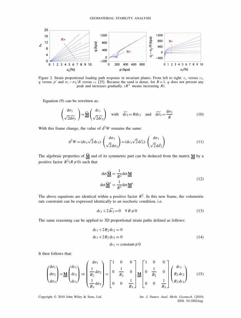
Figure 2. Strain proportional loading path response in invariant planes. From left to right: εv versus ε1,q versus p′ and �1−�3/R versus ε1 [25]. Because the sand is dense, for R=1, q does not present any

peak and increases gradually. (R+ means increasing R).

Equation (9) can be rewritten as:(d�1

√2d�3

)=M

(dε1

√2dε3

)with dε3= Rdε3 and d�3= d�3

R(10)

With this frame change, the value of d2W remains the same:

d2W = (dε1√2dε3)·

(d�1√2d�3

)= (dε1

√2dε3)·

(d�1√2d�3

)(11)

The algebraic properties of M and of its symmetric part can be deduced from the matrix M by a

positive factor R2(R �=0) such that

detM = 1

R2detM

detMs = 1

R2 detMs

(12)

The above equations are identical within a positive factor R2. In this new frame, the volumetricrate constraint can be expressed identically to an isochoric condition, i.e.

dε1+2 dε3=0 ∀ R �=0 (13)

The same reasoning can be applied to 3D proportional strain paths defined as follows:

dε1+2R2 dε2 = 0

dε1+2R3 dε3 = 0

dε1 = constant �=0

(14)

It then follows that:

⎛⎜⎝d�1

d�2

d�3

⎞⎟⎠=M

⎛⎜⎝dε1

dε2

dε3

⎞⎟⎠⇒

⎛⎜⎜⎜⎜⎜⎝d�1

1

R2d�2

1

R3d�3

⎞⎟⎟⎟⎟⎟⎠=

⎡⎢⎢⎢⎢⎢⎣1 0 0

01

R20

0 01

R3

⎤⎥⎥⎥⎥⎥⎦M

⎡⎢⎢⎢⎢⎢⎣1 0 0

01

R20

0 01

R3

⎤⎥⎥⎥⎥⎥⎦⎛⎜⎝ dε1

R2 dε2

R3 dε3

⎞⎟⎠ (15)

Copyright � 2010 John Wiley & Sons, Ltd. Int. J. Numer. Anal. Meth. Geomech. (2010)DOI: 10.1002/nag

F. LAOUAFA ET AL.

We can thus rewrite Equation (15) as:⎛⎜⎜⎝d�1

d�2

d�3

⎞⎟⎟⎠=M

⎛⎜⎜⎝dε1

dε2

dε3

⎞⎟⎟⎠ with dεi = Ridεi and d�i = d�iRi

, i ∈{2,3} (16)

The algebraic properties of M and of its symmetric part can be deduced from the matrix M by

a factor R22R

23(Ri �=0, i ∈{2,3})

detM = 1

R22R

23

detM

detMs = 1

R22 R

23

detMs(17)

We observe that we indeed have the condition of no volume change, i.e.

dε1+ dε2+ dε3=0 ∀Ri �=0, i ∈{2,3} (18)

For this kind of loading, the condition of nullity of d2W is linked to the value of the determinantof the constitutive tensor’s symmetric part. We have seen that instability (and the related diffusefailure mode) at q peak in undrained axisymmetric conditions for a loose sand also exists moregenerally for axisymmetric proportional strain paths at (�1−�3/R) peak. These results themselvescan also be generalized for 3D proportional strain path (�1−�2/R2−�3/R3) peaks. For 2Dconditions, we obtain cones of unstable stress directions (according to different values of Rassociated with ((�1−�3/R) peaks), whereas for 3D conditions elliptical cones have been obtainedfor incrementally piece-wise linear constitutive relations [21].

3. PROPORTIONAL STRESS PATHS. A COMPARISON BETWEEN EXPERIMENTS ANDAN INCREMENTALLY NONLINEAR CONSTITUTIVE RELATION

3.1. Experimental program

The experimental program considered throughout this section consists of two types of tests carriedout on the same material. The first series concerns the constant shear drained (CSD) test afteran initial conventional drained triaxial compression. The second series is a generalization of theprevious ones for different values of the stress ratio and corresponds to proportional shear drained(PSD) tests. The notion of failure discussed in the previous sections is investigated using theseexperimental tests.

3.1.1. Tested material and sample preparation. In order to experimentally study the occurrenceof a diffuse mode of failure, it is convenient to choose a small void ratio value e=Vs/Vv, whereVs is the volume of the solid phase and Vv is the volume of the voids (equal to the volume ofthe water phase because the sample is fully saturated). Moreover, a slenderness ratio (defined ash/d, where h is the height and d the diameter of the cylindrical specimen) of one combined withenlarged frictionless plates and free ends are used at the bottom and at the top so as to prevent thelocalization of deformation. To obtain a large void ratio value, the grain size distribution has to beas uniform as possible, meaning that the grains are nearly of the same size. The chosen materialis Hostun sand. This sand, widely used in France, contains 99.2% silica. The characteristics ofthe sand are summarized in Table I. A 0.2-mm thick latex membrane is used and filled with sandusing the moist tamping method. As the aim of this study is to compare several loading pathsfor approximately the same initial material, i.e. for similar initial void ratios, the existence ofa possible microstructure anisotropy induced by this method does not influence the comparisonas long as the method used for preparing specimens (especially filling the mould) is the same.

Copyright � 2010 John Wiley & Sons, Ltd. Int. J. Numer. Anal. Meth. Geomech. (2010)DOI: 10.1002/nag

GEOMATERIAL STABILITY ANALYSIS

Table I. Basic properties of Hostun S28 sand.

Type Mean size d50(mm) Cu Specific density Max. void ratio Min. void ratio Friction angle (◦)

Quartzic 0.33 2 2.65 1 0.656 32

The sand with a moisture content of approximately 3% is gently compacted inside the mould toreach the maximum void ratio (emax≈1) before isotropic consolidation. To obtain homogeneoussamples, the sand is carefully placed in five successive layers in the mould, as described by Chu andLeong [26]. The membrane is sealed at the base of the cell and at the top cap. A small vacuum isflushed without exceeding 30 kPa. De-aired water percolation is then carried out to ensure samplesaturation. Finally, both cell pressure and back pressure are increased simultaneously step by step.During this process, the B-Skempton coefficient is checked and the samples are assumed to besaturated if B exceeds 98%.

3.1.2. Equipment used. Two digital pressure–volume controllers (DPVC) were used, one for theexternal (cell) pressure and the other for the internal (pore) pressure. A DPVC controls pressureor volume and measures volume variation or pressure variation, respectively. It can easily beconnected to a personal computer via a serial port (RS232) for full control using an in-housesoftware. The pore pressure applied by the DPVC was checked using a pore pressure transducerconnected to the PC. Axial displacements were measured using the linear voltage displacementtransducer (LVDT). The range of displacement is 10mm and the accuracy is about 10�m. Theaxial force is measured at the top of the sample using a submersible load cell so that no correctionhas to be taken into account for the friction between the piston and the chamber. As the transducerwas calibrated in a small range of the 5 kN load cell, the accuracy of the axial force measurementwas 0.3N. To impose the external loading, the apparatus used was an electromechanical load frameZwick� Allround Line 100 kN. The accuracy of the displacement of the frame is 2�m and itsnominal speed is 750mm/min.

3.2. Testing program

All test specimens first underwent isotropic compression to the desired initial confining pressure.Pore pressures are monitored from a calibrated pore water pressure (pw) transducer. The drainagevalve is open during the tests and the specimens were sheared under constant total radial stressand pore water pressure, i.e. under constant effective radial stress.

3.2.1. CSD tests. The objective of this stress path is to simulate the loading of soils within aslope or an embankment when a small increase in pore pressure occurs. The small pore pressureincrease indicates that the material behaves under drained conditions, i.e. with volume changes.This type of test consists of shearing the specimen up to a prescribed stress ratio along a drainedcompression triaxial path and then in loading the specimen under constant deviatoric stress.

Contrary to Sasitharan et al. [27], Di Prisco and Imposimato [28] and Gajo [29], who haveimposed an increase in pore pressure (pw) under constant total stresses to perform the constantshear stress path, we imposed a constant pore water pressure and decreased the total stresses(Figure 3). The above-cited researchers used either dead loads via a plate or a pneumatic chamberto apply the axial force. In our testing program, an electromechanical loading frame is employedas described in the previous section.

More specifically, the sample is first isotropically consolidated to a given initial effective meanpressure. The sample is immediately sheared up to the desired stress ratio under drained conditions,allowing a volumetric variation. For this load-controlled test, the axial load is maintained constantwhen the target value is reached. The total radial pressure is slowly decreased, and therefore thetotal axial stress is dropped by the same quantity as �1=�3+q where q= F/S and S is the actualsection of the sample.

Decreasing the total stress results in a dilation of the sample. Keeping the pore pressure constantduring CSD loading (where �3 decreases) implies that water must be introduced inside the specimen

Copyright � 2010 John Wiley & Sons, Ltd. Int. J. Numer. Anal. Meth. Geomech. (2010)DOI: 10.1002/nag

F. LAOUAFA ET AL.

Figure 3. Control parameters applied to loose Hostun sand at an initial effective mean pressure p′0=300kPa

(CSD test). External load (F), total axial and radial stress and pore water pressure are given versus time.The total stress difference is constant during this test. The load cannot be maintained constant at collapse.

Figure 4. Control parameters versus time applied to loose Hostun sand at an initial effective mean pressurep′0=100kPa (PSD test). External load (F), total axial and radial stress and pore water pressure are given

versus time. The total stress difference increases during this test.

to counterbalance the drop in pore pressure as the sample dilates. The volumetric changes arerecorded as the test is conducted under drained conditions.

3.2.2. PSD tests. This test can be viewed as a generalization of the CSD test. Indeed, during thePSD test, the axial load is not maintained constant after the shearing path, but linearly evolves.As for the CSD test, we imposed a constant pore water pressure and decreased the total stresses(Figure 4). After the isotropic consolidation to a given initial effective mean pressure, the sample isimmediately sheared up to the desired stress ratio under drained conditions, allowing a volumetricvariation. For this load-controlled test, the axial load is increased until the target value is reached.The total radial pressure is slowly decreased. Depending on the axial force rate increase or decreaseand the radial stress rate decrease, the axial stress rate can be positive or negative, leading to anincrease or decrease in the axial stress.

Copyright � 2010 John Wiley & Sons, Ltd. Int. J. Numer. Anal. Meth. Geomech. (2010)DOI: 10.1002/nag

GEOMATERIAL STABILITY ANALYSIS

-1.5

-1

-0.5

0

0.5

1

1.5

2

0

10

20

30

40

50

60

0

ε 1 &

εv

(%)

q (k

Pa)

t (s)

A

A

A

B

B

B

C

C

C

q

ε1

εv

200 400 600 800 1000 1200 1400 1600 1800 2000 2200 2400

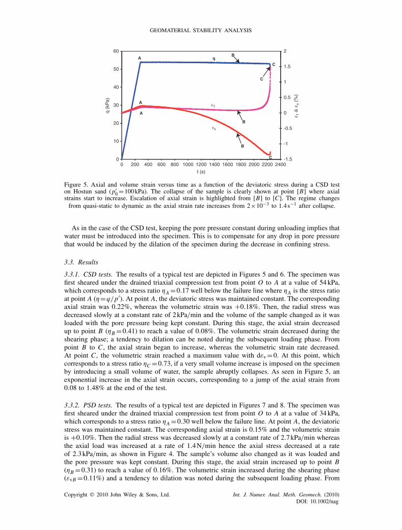
Figure 5. Axial and volume strain versus time as a function of the deviatoric stress during a CSD teston Hostun sand (p′

0=100kPa). The collapse of the sample is clearly shown at point [B] where axialstrains start to increase. Escalation of axial strain is highlighted from [B] to [C]. The regime changesfrom quasi-static to dynamic as the axial strain rate increases from 2×10−3 to 1.4s−1 after collapse.

As in the case of the CSD test, keeping the pore pressure constant during unloading implies thatwater must be introduced into the specimen. This is to compensate for any drop in pore pressurethat would be induced by the dilation of the specimen during the decrease in confining stress.

3.3. Results

3.3.1. CSD tests. The results of a typical test are depicted in Figures 5 and 6. The specimen wasfirst sheared under the drained triaxial compression test from point O to A at a value of 54 kPa,which corresponds to a stress ratio �A =0.17 well below the failure line where �A is the stress ratioat point A (�=q/p′). At point A, the deviatoric stress was maintained constant. The correspondingaxial strain was 0.22%, whereas the volumetric strain was +0.18%. Then, the radial stress wasdecreased slowly at a constant rate of 2kPa/min and the volume of the sample changed as it wasloaded with the pore pressure being kept constant. During this stage, the axial strain decreasedup to point B (�B =0.41) to reach a value of 0.08%. The volumetric strain decreased during theshearing phase; a tendency to dilation can be noted during the subsequent loading phase. Frompoint B to C , the axial strain began to increase, whereas the volumetric strain rate decreased.At point C , the volumetric strain reached a maximum value with dεv=0. At this point, whichcorresponds to a stress ratio �C =0.73, if a very small volume increase is imposed on the specimenby introducing a small volume of water, the sample abruptly collapses. As seen in Figure 5, anexponential increase in the axial strain occurs, corresponding to a jump of the axial strain from0.08 to 1.48% at the end of the test.

3.3.2. PSD tests. The results of a typical test are depicted in Figures 7 and 8. The specimen wasfirst sheared under the drained triaxial compression test from point O to A at a value of 34 kPa,which corresponds to a stress ratio �A =0.30 well below the failure line. At point A, the deviatoricstress was maintained constant. The corresponding axial strain is 0.15% and the volumetric strainis +0.10%. Then the radial stress was decreased slowly at a constant rate of 2.7kPa/min whereasthe axial load was increased at a rate of 1.4N/min hence the axial stress decreased at a rateof 2.3kPa/min, as shown in Figure 4. The sample’s volume also changed as it was loaded andthe pore pressure was kept constant. During this stage, the axial strain increased up to point B(�B =0.31) to reach a value of 0.16%. The volumetric strain increased during the shearing phase(εvB =0.11%) and a tendency to dilation was noted during the subsequent loading phase. From

Copyright � 2010 John Wiley & Sons, Ltd. Int. J. Numer. Anal. Meth. Geomech. (2010)DOI: 10.1002/nag

F. LAOUAFA ET AL.

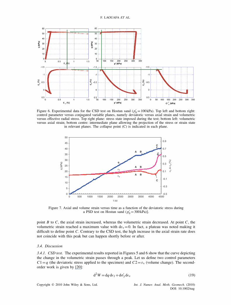
Figure 6. Experimental data for the CSD test on Hostun sand (p′0=100kPa). Top left and bottom right:

control parameter versus conjugated variable planes, namely deviatoric versus axial strain and volumetricversus effective radial stress. Top right plane: stress state imposed during the test; bottom left: volumetricversus axial strain; bottom centre: intermediate plane allowing the projection of the stress or strain state

in relevant planes. The collapse point (C) is indicated in each plane.

0

5

10

15

20

25

30

35

40

45

50

0

t (s)

q (k

Pa)

-0.5

-0.3

-0.1

0.1

0.3

0.5

0.7

0.9

ε 1 &

εv

(%)

A

A

A

B

B

B

C

C

C

q

ε1

εv

500 1000 1500 2000 2500 3000 3500 4000 4500

Figure 7. Axial and volume strain versus time as a function of the deviatoric stress duringa PSD test on Hostun sand (p′

0=300kPa)].

point B to C , the axial strain increased, whereas the volumetric strain decreased. At point C , thevolumetric strain reached a maximum value with dεv=0. In fact, a plateau was noted making itdifficult to define point C . Contrary to the CSD test, the high increase in the axial strain rate doesnot coincide with this peak but can happen shortly before or after.

3.4. Discussion

3.4.1. CSD test. The experimental results reported in Figures 5 and 6 show that the curve depictingthe change in the volumetric strain passes through a peak. Let us define two control parametersC1=q (the deviatoric stress applied to the specimen) and C2=εv (volume change). The second-order work is given by [20]:

d2W =dq dε1+d�′3 dεv (19)

Copyright � 2010 John Wiley & Sons, Ltd. Int. J. Numer. Anal. Meth. Geomech. (2010)DOI: 10.1002/nag

GEOMATERIAL STABILITY ANALYSIS

Figure 8. Experimental data for the PSD test on Hostun sand (p′0=300kPa). Top left and bottom right:

deviatoric stress versus axial strain and volumetric strain versus effective radial stress. Top right plane:stress state imposed during the test; bottom left: volumetric versus axial strain; bottom centre: plane

allowing the projection of the stress or strain states in relevant planes.

For the CSD tests, the deviatoric stress is maintained constant (dq=0), so that dC1=0 during thetest. Furthermore, the second-order work, along this particular loading path, reads:

d2W =d�′3 dεv (20)

Five plots are presented in Figure 6 to provide a full understanding of the mechanical behaviourof the specimen before and just after collapse. The conjugated variables of C1 and C2 are,respectively, ε1 (axial strain) and �′

3 (effective radial stress). Hence, the top left plane of Figure 6corresponds to the (ε1,q) plane, whereas the bottom left corresponds to the (�′

3,εv). The top rightplane (p′,q) corresponds to the stress state imposed during the test, whereas the two last planesgive the response to the loading.

Figure 6 shows the experimental data plotted in various spaces to fully understand the mechanicalbehaviour of the specimen before and after collapse occurs. It is reminded that it is importantto plot the data in the appropriate space involving the control variables C1 and C2 and theirconjugates, ε1 (axial strain) and �′

3 (effective confining stress), respectively, in order to pin-pointthe exact bifurcation point. As Equation (20) indicates, the second-order work vanishes wheneverd�′

3/dεv=0, hence at the peak of the volumetric strain as confirmed in the bottom right sub-plotof Figure 6. The other sub-plots in Figure 6 essentially highlight the existence of a peak in thevolumetric strain also found in combination with other parameters and the linkage with the controlvariables defining the loading programme in the CSD test.

As anticipated, beyond the peak in the dεv versus �′3 plot in Figure 6, the second-order work

becomes necessarily negative so that if any perturbation was to be applied to the specimen,an abrupt collapse would occur. Experimentally, an infinitesimal perturbation is applied to thesecond control parameter C2=εv. More specifically, a very small value of dC2 was imposed tocounterbalance the pore pressure decrease, as indicated in the previous section, and correspondsto a very small volume increase. Under the effect of this infinitesimal perturbation, the axial strainabruptly increases, leading to the total collapse of the sample. The second-order work per unit ofvolume computed using the data is also plotted versus time in Figure 9. The second-order work has

Copyright � 2010 John Wiley & Sons, Ltd. Int. J. Numer. Anal. Meth. Geomech. (2010)DOI: 10.1002/nag

F. LAOUAFA ET AL.

-1.5

-1

-0.5

0

0.5

0

t (sec)

d2 W (

J/m

3 )-1.5

-1

-0.5

0

0.5

500 1000 1500 2000 2500

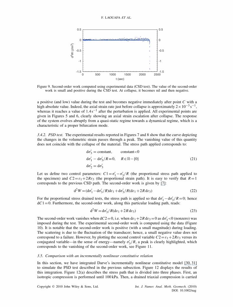
Figure 9. Second-order work computed using experimental data (CSD test). The value of the second-orderwork is small and positive during the CSD test. At collapse, it becomes nil and then negative.

a positive (and low) value during the test and becomes negative immediately after point C with ahigh absolute value. Indeed, the axial strain rate just before collapse is approximately 2×10−3 s−1,whereas it reaches a value of 1.4s−1 after the perturbation is applied. All experimental points aregiven in Figures 5 and 6, clearly showing an axial strain escalation after collapse. The responseof the system evolves abruptly from a quasi-static regime towards a dynamical regime, which is acharacteristic of a proper bifurcation mode.

3.4.2. PSD test. The experimental results reported in Figures 7 and 8 show that the curve depictingthe changes in the volumetric strain passes through a peak. The vanishing value of this quantitydoes not coincide with the collapse of the material. The stress path applied corresponds to:

d�′3 = constant, constant<0

d�′1 − d�′

3/R=0, R∈R−{0}d�′

2 = d�′3

(21)

Let us define two control parameters: C1=�′1−�′

3/R (the proportional stress path applied tothe specimen) and C2=ε1+2Rε3 (the proportional strain path). It is easy to verify that R=1corresponds to the previous CSD path. The second-order work is given by [7]:

d2W = (d�′1−d�′

3/R)dε1+d�′3/R(dε1+2Rdε3) (22)

For the proportional stress drained tests, the stress path is applied so that d�′1−d�′

3/R=0; hencedC1=0. Furthermore, the second-order work, along this particular loading path, reads:

d2W =d�′3/R(dε1+2Rdε3) (23)

The second-order work vanishes when dC2=0, i.e. when dε1+2Rdε3=0 as d�′3<0 (nonzero) was

imposed during the test. The experimental second-order work is computed using the data (Figure10). It is notable that the second-order work is positive (with a small magnitude) during loading.The scattering is due to the fluctuation of the transducer; hence, a small negative value does notcorrespond to a failure. However, by plotting the second control variable C2=ε1+2Rε3 versus itsconjugated variable—in the sense of energy—namely �′

3/R, a peak is clearly highlighted, whichcorresponds to the vanishing of the second-order work, see Figure 11.

3.5. Comparison with an incrementally nonlinear constitutive relation

In this section, we have integrated Darve’s incrementally nonlinear constitutive model [30, 31]to simulate the PSD test described in the previous subsection. Figure 12 displays the results ofthis integration. Figure 12(a) describes the stress path that is divided into three phases. First, anisotropic compression is performed until 100 kPa. Then, a drained triaxial compression is carried

Copyright � 2010 John Wiley & Sons, Ltd. Int. J. Numer. Anal. Meth. Geomech. (2010)DOI: 10.1002/nag

GEOMATERIAL STABILITY ANALYSIS

-0.1

-0.05

0

0.05

0.1

0.15

0.2

0

t (sec)

d2 W (

J/m

3)

-0.1

-0.05

0

0.05

0.1

0.15

0.2

500 1000 1500 2000 2500 3000 3500 4000 4500 5000

Figure 10. Second-order work computed using experimental data (PSD test). The value of the second-orderwork is small and positive during the PSD test. At the peak, it becomes nil and then negative.

Figure 11. The conjugated variables with respect to the energy in the PSD test: Top:�′1−�′

3/R versus ε1; bottom: ε1+2Rε3 versus �′3/R. For the latter, the peak corresponds

to the vanishing of the second-order work.

out until a deviatoric stress of 35 kPa is reached. Finally, a proportional stress path as defined inEquation (21) is applied. In the present case, the parameter R is about 1.18. Figures 12(b) and (c)present the deviatoric as well as the volume change responses of the sample. The change in the

Copyright � 2010 John Wiley & Sons, Ltd. Int. J. Numer. Anal. Meth. Geomech. (2010)DOI: 10.1002/nag

F. LAOUAFA ET AL.

70 75 80 85 90 95 100 105 110 1150

5

10

15

20

25

30

35

40

45

experiemental

INL

p (kPa)

q (k

Pa)

0 0.1 0.2 0.3 0.4 0.5 0.6 0.7

0 0.1 0.2 0.3 0.4 0.5 0.6 0.7

0

5

10

15

20

25

30

35

40

45

q (k

Pa)

ε1 (%)

-0.25

-0.2

-0.15

-0.1

-0.05

0

ε1 (%)

ε v (%

)

Figure 12. Comparison of Darve’s incrementally nonlinear model with the PSD test results.

loading path from the triaxial to the proportional phases is obvious in Figure 12(c) for ε1=0.15%,and can be observed in Figure 12(b) with the discontinuous slope change for q≈36kPa.

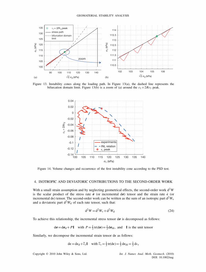
The main goal of this section is to highlight the existence of a bifurcation domain for nonasso-ciated materials in which failure can occur before reaching the plasticity limit condition. After adrained triaxial compression, which is stopped before entering the bifurcation domain (see Figure12(a)), the loading path described in Equation (21) is then followed with R≈1.18. This loadingdirection makes it possible to cross the bifurcation limit. As this limit is reached, instability cones aregrowing. Nevertheless, for the loading path considered, collapse is possible only when the loadingdirection matches a direction included in a cone. In fact, when the second-order work vanishes atthe peak of ε1+2Rε3, the loading direction is just at the limit of a cone (see Figure 12(b)). Theboundaries of these cones are given by the equation d2W =0. Outside the cones d2W>0, and inside,d2W<0. Furthermore, as mentioned above, the collapse at the ε1+2Rε3 peak is effective only if thevariable dε1+2Rdε3 is controlled. If this is not the case, the loading path can be followed withoutfailure occurring. Nevertheless, after such a peak, the loading path is unstable. A slight disturbancein the controlled parameters, for example, leads to the collapse of the sample (Figure 13).

On the other hand, we emphasize that for the present PSD test, no instability or failure ispossible at the εv peak. As presented in Figure 14, the εv peak is reached before the ε1+2Rε3 peakcorresponding to the vanishing of the second-order work. From an experimental point of view, onemust be aware of this, because when the R parameter is not very different from 1 it may not beeasy to distinguish the εv peak from the ε1+2Rε3 peak, as can be seen in Figure 14. Hence, it isimportant to note that theoretically, an extremum in the volume change is not synonymous withan unstable state.

Copyright � 2010 John Wiley & Sons, Ltd. Int. J. Numer. Anal. Meth. Geomech. (2010)DOI: 10.1002/nag

GEOMATERIAL STABILITY ANALYSIS

90 100 110 120 130 140

100

105

110

115

120

125

130

135

stress path

bifurcation domainlimit

zoom

σ 1 (k

Pa)

102 103 104 105 106

110.5

111

111.5

112

112.5

113

113.5

114

σ 1 (k

Pa)

1 + 2R 3 peak

(a) (b)

Figure 13. Instability cones along the loading path. In Figure 13(a), the dashed line represents thebifurcation domain limit. Figure 13(b) is a zoom of (a) around the ε1+2Rε3 peak.

100 105 110 115 120 125 130 135 140-0.14

-0.12

-0.1

-0.08

-0.06

-0.04

-0.02

0

0.02

0.04

σ1 (kPa)

ε 1 +

2R

ε 3

experiments

INL relationεv peak

Figure 14. Volume changes and occurrence of the first instability cone according to the PSD test.

4. ISOTROPIC AND DEVIATORIC CONTRIBUTIONS TO THE SECOND-ORDER WORK

With a small strain assumption and by neglecting geometrical effects, the second-order work d2Wis the scalar product of the stress rate r (or incremental dr) tensor and the strain rate ε (orincremental dε) tensor. The second-order work can be written as the sum of an isotropic part d2Wvand a deviatoric part d2Wd of each rate tensor, such that:

d2W =d2Wv+d2Wd (24)

To achieve this relationship, the incremental stress tensor dr is decomposed as follows:

dr=drd+PI with P= 13 tr(dr)= 1

3drkk, and I is the unit tensor

Similarly, we decompose the incremental strain tensor dε as follows:

dε=dεd+ εvI with εv= 13 tr(dε)= 1

3 dεkk= 13 dεv

Copyright � 2010 John Wiley & Sons, Ltd. Int. J. Numer. Anal. Meth. Geomech. (2010)DOI: 10.1002/nag

F. LAOUAFA ET AL.

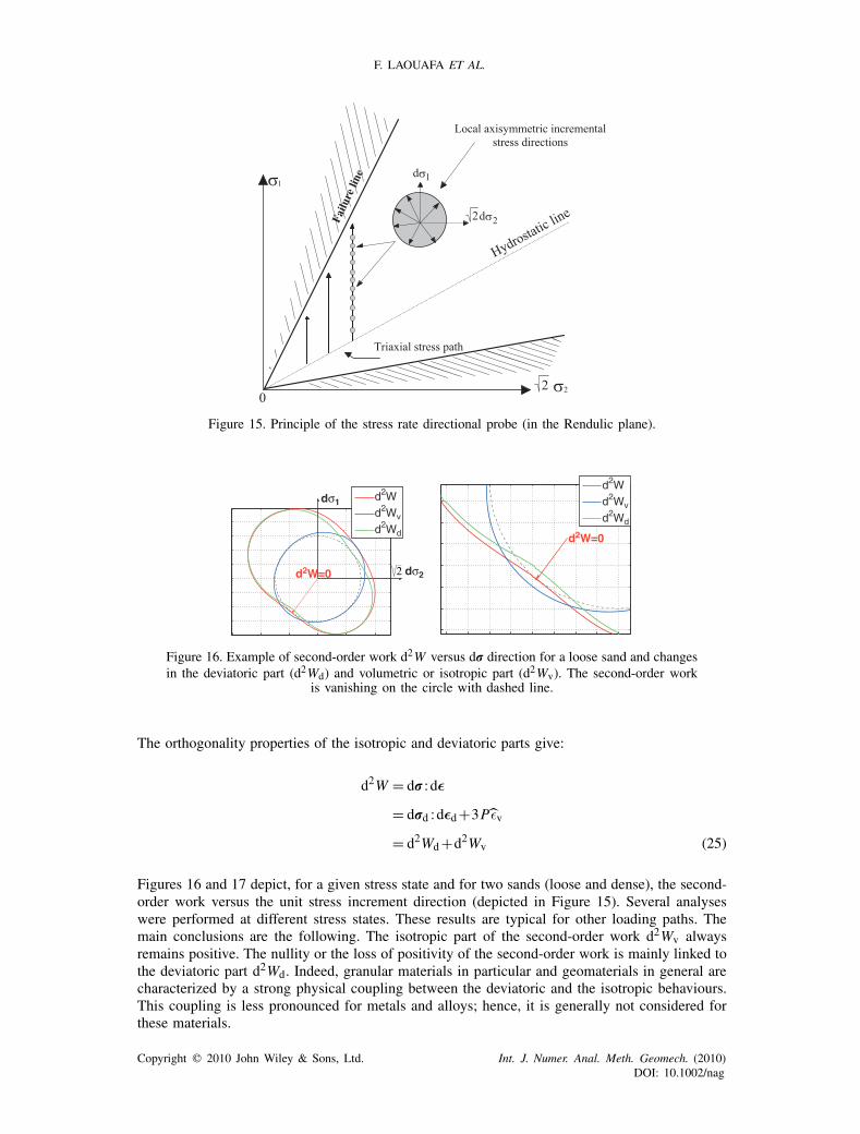
Figure 15. Principle of the stress rate directional probe (in the Rendulic plane).

2 dσ2d2W=0

d2W=0

d2Wv

d2W

d2Wd

d2Wv

d2W

d2Wd

dσ1

Figure 16. Example of second-order work d2W versus dr direction for a loose sand and changesin the deviatoric part (d2Wd) and volumetric or isotropic part (d2Wv). The second-order work

is vanishing on the circle with dashed line.

The orthogonality properties of the isotropic and deviatoric parts give:

d2W = dr : dε

= drd :dεd+3 Pεv

= d2Wd+d2Wv (25)

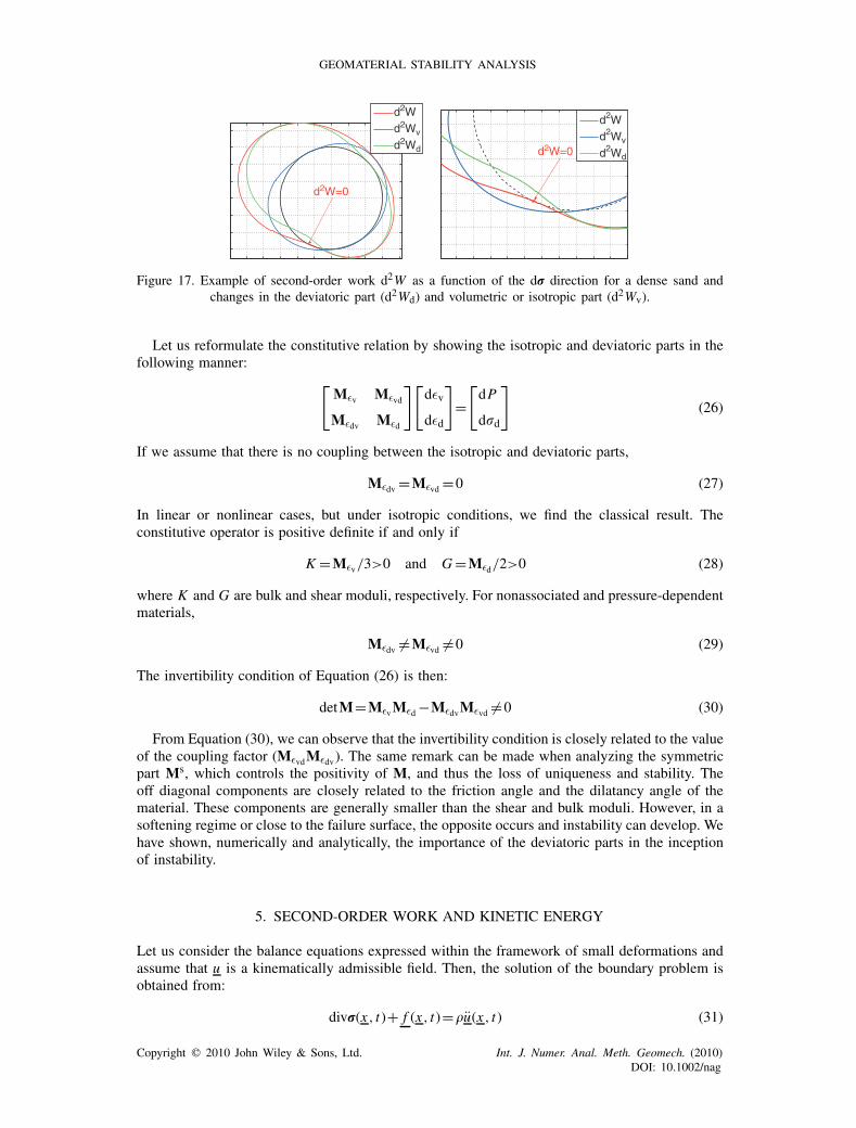
Figures 16 and 17 depict, for a given stress state and for two sands (loose and dense), the second-order work versus the unit stress increment direction (depicted in Figure 15). Several analyseswere performed at different stress states. These results are typical for other loading paths. Themain conclusions are the following. The isotropic part of the second-order work d2Wv alwaysremains positive. The nullity or the loss of positivity of the second-order work is mainly linked tothe deviatoric part d2Wd. Indeed, granular materials in particular and geomaterials in general arecharacterized by a strong physical coupling between the deviatoric and the isotropic behaviours.This coupling is less pronounced for metals and alloys; hence, it is generally not considered forthese materials.

Copyright � 2010 John Wiley & Sons, Ltd. Int. J. Numer. Anal. Meth. Geomech. (2010)DOI: 10.1002/nag

GEOMATERIAL STABILITY ANALYSIS

d2W=0

d2Wv

d2W

d2Wd d2W=0d2Wv

d2W

d2Wd

Figure 17. Example of second-order work d2W as a function of the dr direction for a dense sand andchanges in the deviatoric part (d2Wd) and volumetric or isotropic part (d2Wv).

Let us reformulate the constitutive relation by showing the isotropic and deviatoric parts in thefollowing manner: [

Mεv Mεvd

Mεdv Mεd

][dεv

dεd

]=[dP

d�d

](26)

If we assume that there is no coupling between the isotropic and deviatoric parts,

Mεdv =Mεvd =0 (27)

In linear or nonlinear cases, but under isotropic conditions, we find the classical result. Theconstitutive operator is positive definite if and only if

K =Mεv/3>0 and G=Mεd/2>0 (28)

where K and G are bulk and shear moduli, respectively. For nonassociated and pressure-dependentmaterials,

Mεdv �=Mεvd �=0 (29)

The invertibility condition of Equation (26) is then:

detM=MεvMεd −MεdvMεvd �=0 (30)

From Equation (30), we can observe that the invertibility condition is closely related to the valueof the coupling factor (MεvdMεdv). The same remark can be made when analyzing the symmetricpart Ms, which controls the positivity of M, and thus the loss of uniqueness and stability. Theoff diagonal components are closely related to the friction angle and the dilatancy angle of thematerial. These components are generally smaller than the shear and bulk moduli. However, in asoftening regime or close to the failure surface, the opposite occurs and instability can develop. Wehave shown, numerically and analytically, the importance of the deviatoric parts in the inceptionof instability.

5. SECOND-ORDER WORK AND KINETIC ENERGY

Let us consider the balance equations expressed within the framework of small deformations andassume that u is a kinematically admissible field. Then, the solution of the boundary problem isobtained from:

divr(x , t)+ f (x, t)=�u(x , t) (31)

Copyright � 2010 John Wiley & Sons, Ltd. Int. J. Numer. Anal. Meth. Geomech. (2010)DOI: 10.1002/nag

F. LAOUAFA ET AL.

Figure 18. Configurations of the slope and loading programs (left); the example induces granular avalanchesin a two-dimensional medium (right).

Let us calculate the time derivative of Equation (31) assuming the density � to be constant.Multiplying the resulting time derivative by the velocity u(x, t) as in a scalar product, we obtainthe following equation:

(divr+ f )· u=�( ˙u)· uSince

�( ˙u · u)=�( ˙(u · u))−�‖u‖2= Ec−�‖u‖2 (32)

where Ec is the kinetic energy, we finally obtain the following relationship:

div(r · u)− r : ε+ f · u= Ec−�‖u‖2 (33)

By rearranging the above equation, it follows that:

d2W =div(r· u)+ f · u− Ec+�‖u‖2 (34)

Indeed, the above equilibrium equation is interesting in that it embeds explicitly the second-orderwork. However, it should be noted that there is no direct relationship between kinetic energy andthe second-order work. Taking into account the inertial terms of �‖u‖2 through damping (viscous,friction or others) seems to be indeed necessary in post failure where there is a transition froma quasi-static regime to a dynamic one. Interestingly, inertial effects may lead to a mathematicalregularization of the problem.

Nicot and Darve [9] have shown, under additional assumptions, a direct link between second-order work and kinetic energy. In this study, the vanishing or negative values of the second-orderwork lead to an increase in kinetic energy. Using the discrete element method, Darve et al. [7] alsoshow that the kinetic energy of the system grows when the global and discrete values of the second-order work become nil or negative. An example of such results is depicted in Figures 18 and 19.

6. EIGENVALUE ANALYSIS

6.1. Relation between the global second-order work and the global tangent operator

At a given material point x of a body � of Rn , n∈{1,2,3}, the second-order work is:

d2W =dr(x) :dε(x ) ∀x ∈�

Copyright � 2010 John Wiley & Sons, Ltd. Int. J. Numer. Anal. Meth. Geomech. (2010)DOI: 10.1002/nag

GEOMATERIAL STABILITY ANALYSIS

Figure 19. Comparison between global second-order work and global kinetic energyas functions of the rotation angle �.

Noting Equation (34) without the dynamic terms, the space integration of d2W over � leads tothe global expression of the second-order work (d2W ), i.e.

d2W =∫

�dr(x) :dε(x)d�=

∫�d f ·du d�+

∫�1

(dr ·n)·du d� (35)

Let us recall that traction (dr ·n) is imposed on the boundary �1 and displacements are imposedon �2, with: �1∩�2=∅. Additional relationships that describe the BVP are as follows:

dε(x )=∇sdu(x) and F(dr(x ),dε(x),�)=0

so that the incremental or rate fields du(x ), dr(x) and dε(x ) are solutions of the BVP.After a classical spatial discretization using the finite element approach, the discrete expression

of Equation (35) becomes:

d2W =∫�dr(x ) :dε(x)d�=∑

e

∑kj ke �k t

e dε(xke)tM(xke)dε(x

ke) (36)

with

dr(xke)=M(xke)dε(xke)

where j ke , �ke are the Jacobian of the transformation computed at the Gauss integration point

k of element e and the corresponding weight (Gauss quadrature), respectively. In the one field(displacement, velocity or incremental displacement) variational formulation, the strain (or strainrate or incremental strain) is expressed as:

dε(xke)=Bke due

The matrix Bke is the classical displacement–strain operator. With the above consideration we

obtain:

d2W =∫

�dr(x) :dε(x)d� =∑

e

∑kj ke �k

e

(tdue

tBketMk

eBke due

)=∑

e

∑k

tdue[ jke �k

etBk

etMk

eBke]due

Copyright � 2010 John Wiley & Sons, Ltd. Int. J. Numer. Anal. Meth. Geomech. (2010)DOI: 10.1002/nag

F. LAOUAFA ET AL.

=∑e

∑k

tdueKke due

=∑e

tdueKe due (37)

= tdUKdU

The matrices Kke , Ke and K are the stiffness matrix computed at the integration point k, the

elementary stiffness matrix and the global stiffness matrix, respectively. We have shown that

d2W =∫�dr(x ) :dε(x)d�= tdUKdU = tdUKs dU = tdU ·dF (38)

because at equilibrium or at rest we have the following equality:

KdU =dF (39)

The global second-order work d2W Equation (35) for a deformable solid �, associated with aset of external disturbances, can be evaluated either by using the general expression or by usingdirectly the second-order work done by the external incremental forces. Let us underline that forincrementally linear problems, the values of the diagonal components Kii represent the globalsecond-order work for a unit incremental displacement of the i th component of the displacementvector:

Kii=

⎛⎜⎜⎜⎜⎜⎜⎜⎜⎝

0

0

1

...

0

⎞⎟⎟⎟⎟⎟⎟⎟⎟⎠

t

·K ·

⎛⎜⎜⎜⎜⎜⎜⎜⎜⎝

0

0

1

...

0

⎞⎟⎟⎟⎟⎟⎟⎟⎟⎠(40)

Also, recall that the stiffness matrix is constructed by summation over integration points and finiteelements ( Equation (38)). As such, any local violation of the second-order work at the integration(Gauss) point level does not necessarily translate into a loss of uniqueness in the solution of theboundary value at the element or structural (global) level. Thus, from this viewpoint, the summationinvolved in a typical finite element assembly process is seen to regularize the BVP. However,if enough integration points violate the second-order work to the point of vanishing the globalsecond-order work, then structural collapse occurs.

We now briefly present some of the properties of d2W . The second-order work d2W , when theconstitutive relation is expressed in the following manner:

ε=D�

is a homogeneous function of degree 2 in �, as a consequence of the homogeneity of degree 0of D. Thus,

d2W (��)=�2 d2W (�) ∀�>0 (41)

Using vectorial notation and according to Euler’s theorem, it follows that:

∑i

�(d2W )

��i�i =∇�(d

2W )· �=2d2W, i ∈{1,2, . . . ,6} (42)

Then

12∇ �(d

2W )· �= t�D�⇒ t�[D�− 12t∇ �(d

2W )]=0 ∀�∈Rn, ‖�‖ �=0 (43)

Copyright � 2010 John Wiley & Sons, Ltd. Int. J. Numer. Anal. Meth. Geomech. (2010)DOI: 10.1002/nag

GEOMATERIAL STABILITY ANALYSIS

Knowing that ε=D�, we finally have

[ε− 12t∇ �(d

2W )]· �=0, ∀�∈Rn, ‖�‖ �=0 (44)

In the case of hyperelastic material, this equation states that:

εij= 1

2

�()��ij

(45)

Here, the second-order work stands for internal energy . By expressing d2W in terms of thestress rate �, we have

d2W = t�Ds�=Dsij�i � j , i, j ∈{1,2, . . . ,6}2 (46)

In the linear case, the equation d2W =1 represents a surface in an Euclidean space of dimension 6. Ifthe constitutive operator Ds is positive definite, the surface is closed and describes a hyper-ellipsoid

centred about the origin in the stress rate space. The gradient (∇ �(d2W )) of the second-order work

represents a vector that is normal to this surface and is expressed by:

∇ �(d2W )=2Ds� with t∇ � =

(�(d2W )

��1, . . . ,

�(d2W )

��n

)(47)

The principal axes of the ellipsoid are orthogonal to the surface and define the eigenvectors ofthe symmetric part Ds of the constitutive operator. In the following section, we will provide aneigenvalue analysis of a linearized BVP. We analyze the displacement field associated with the first(in a monotonously increasing loading) vanishing eigenvalue of the symmetric part of the globaltangent operator and we compare it with the displacement field at failure, defined by the loss ofconvergence of the Newton–Raphson algorithm.

6.2. Modal analysis of the symmetric part of the tangent operator

Because of the relationship in Equation (39), the global formulation is somewhat identical to thelocal one. That is why it is interesting to study the eigenvalues and eigenvectors of the symmetricpartKs ofK. Nevertheless, considering elasto-plastic materials, the global problem is more complexto analyze. In fact, as a result of the constitutive relation, the K operator is incrementally nonlinearand depends on the global direction dU or dF . Thus, even for a coarse discretization, it is uselessto look for every possible unstable loading direction for a given equilibrium state. Furthermore,when the determinant ofKs vanishes, a first global unstable direction exists for the tangent operatordescribing Hill’s linear comparison solid. Even if nothing guarantees that this loading direction canbe physically reached for the boundary conditions considered, it can be interesting to investigate it.

In the following, a heuristic case of a soil slope loaded by a shallow foundation is analyzed.This problem could describe the effect of a road or a building transferring loads in the middlesection of a slope. The geometry as well as the boundary conditions are presented in Figure 20.The computations were performed with the finite element code Lagamine [32] and the constitutivemodel Plasol [33]. A brief description of this model can be also found in [22, 34]. The mainproperties of the soil are summarized in Table II. Figure 21 shows the mesh deformation at the laststep before divergence of the computations. The traction increment imposed at each step is 50 kPa,and at the first step, only gravity is applied. Hence, the total stress imposed on the foundation atstep 30 is 1450 kPa. Long before this step, which is assumed to be the ultimate equilibrium statebefore the physical collapse of the slope, the determinant of Ks vanishes at step 8. Figure 22 showsthe lowest eigenvalues of Ks during the loading. Therefore, considering the tangent operator atstep 8, an incremental displacement dU∗ oriented in the direction as eigenvector V0 associatedwith the vanishing eigenvalue �0 leads to a nil global second-order work. The main difficulty isthat for an equilibrium state 8, a vector dU∗ will probably change the operator K because of itsincrementally piece-wise linearity. In this condition, V0 has no physical meaning. Nevertheless,we have represented this eigenvector V0, and we observe that it is almost collinear to the last

Copyright � 2010 John Wiley & Sons, Ltd. Int. J. Numer. Anal. Meth. Geomech. (2010)DOI: 10.1002/nag

F. LAOUAFA ET AL.

108 m

41 m 41 m10 m 6 m

40 m

15 m

15 m

dp = 50kPa

Figure 20. Finite element mesh used in the heuristic nonlinear computations. Vertical boundaries are fixedin the horizontal direction, whereas the horizontal bottom boundary is fixed in the vertical direction.

Table II. Soil properties of the slope.

E=95MPa C=30kPa

=0.21 =20◦�=2740kg/m3 �=5◦

Figure 21. Deformed mesh at the last step before the divergence of the computation for this heuristic case.

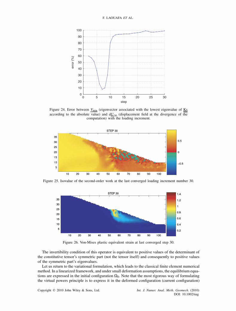
incremental displacement field before the divergence at step 30 (see Figure 23). This means thatthis eigenvector V0 seems to describe the failure mechanism well in this simulation. Similar resultswere also observed by Prunier et al. [22] with the same FEM code and elasto-plastic model, butfor other heuristic cases. From a quantitative point of view, we have defined a function to measurethe deviation between any two vectors (V1 and V2) of Rn :

er(V1,V2)=(1−

∣∣∣∣∣ tV1.V2‖V1‖.‖V2‖

∣∣∣∣∣)

·100 (48)

When er(V1,V2)=0%, both vectors are collinear, and they are perpendicular when er(V1,V2)=100%. With the help of this function, the deviation evolves between the last incremental displace-ment dU30 at step 30 and the eigenvector related to the lowest eigenvalue (in relation with itsabsolute value) Vmin has been plotted in Figure 24. It should be noted that at step 8, Vmin isexactly equal to V0. It is interesting to see that the minimum of this function is reached at the timewhen the first eigenvalue vanishes. Furthermore, according to the function of Equation (48), thedeviation error between V0 and dU30 is less than 10%.

Finally, the last two results presented on this simulation are the isovalues of the local second-orderwork and of the Von-Mises plastic equivalent strain at step 30. The first result (Figure 25) givesa good idea of the unstable zones immediately prior to the effective failure. A set of consecutivepictures of these isovalues along the loading program would show how the unstable zones evolve.The second results (Figure 26) provide a view of the failure mechanism according to the meshconsidered. This area is quite well described either by the final incremental displacement dU30 orthe eigenvector V0 (see Figure 23).

Copyright � 2010 John Wiley & Sons, Ltd. Int. J. Numer. Anal. Meth. Geomech. (2010)DOI: 10.1002/nag

GEOMATERIAL STABILITY ANALYSIS

0 5 10 15 20 25 302

1

0

1

2

3

4x 106

increment

eige

nval

ues

Figure 22. Lowest eigenvalues of Ks with loading increment.

0 10 20 30 40 50 60 70 80 90 1000

5

10

15

20

25

30

35

40eigenvector of Ms

total displacement

Figure 23. Comparison of the eigenvector associated with the first vanishing eigenvalue of Ks and thedisplacement rate vector at failure state.

6.3. A remark on finite elements and instability analyses

In the stability analysis of BVPs (like the previous one), using the second-order work criterion, aquestion arises. Consider a deformable solid subject to kinematical constraints avoiding rigid bodymotion and to incremental tractions (dg) on its boundary:

dr ·n=dg

such that the direction of the external tractions (external loading) coincides with an unstabledirection in the sense of d2W . Some computations in this configuration will converge with no lossof uniqueness. This may contradict the stability criterion based on the sign of the second-orderwork (global or local). If we exclude the case of flutter instability, the explanation is relativelysimple. It has been demonstrated and observed experimentally (for some feasible loading paths)that when d2W is zero, at least one external loading made up of mixed (or unmixed) componentsof the stress rate and strain rate exists, which leads to loss of uniqueness and loss of stability.

As was shown for proportional strain or stress paths, the new operator defines a mapping betweenthe mixed loading space and the second-order work conjugated mixed response space.

Copyright � 2010 John Wiley & Sons, Ltd. Int. J. Numer. Anal. Meth. Geomech. (2010)DOI: 10.1002/nag

F. LAOUAFA ET AL.

0 5 10 15 20 25 300

10

20

30

40

50

60

70

80

90

100

step

erro

r (%

)

Figure 24. Error between Vmin (eigenvector associated with the lowest eigenvalue of Ksaccording to the absolute value) and dU 30 (displacement field at the divergence of the

computation) with the loading increment.

Figure 25. Isovalue of the second-order work at the last converged loading increment number 30.

Figure 26. Von-Mises plastic equivalent strain at last converged step 30.

The invertibility condition of this operator is equivalent to positive values of the determinant ofthe constitutive tensor’s symmetric part (not the tensor itself) and consequently to positive valuesof the symmetric part’s eigenvalues.

Let us return to the variational formulation, which leads to the classical finite element numericalmethod. In a linearized framework, and under small deformation assumptions, the equilibrium equa-tions are expressed in the initial configuration �0. Note that the most rigorous way of formulatingthe virtual powers principle is to express it in the deformed configuration (current configuration)

Copyright � 2010 John Wiley & Sons, Ltd. Int. J. Numer. Anal. Meth. Geomech. (2010)DOI: 10.1002/nag

GEOMATERIAL STABILITY ANALYSIS

�t . If we call W the power of internal stress, then

W =∫

�t

r :Dd� (49)

with r Cauchy stress tensor and D the rate of deformationD= 12 (

t(∇v)+(∇v)). These two variablesr and D are conjugated in the power sense W . This invariant must be independent of the choice ofthe measure and reference frame of stresses and strains. For a given choice of stress, the associatedstrain must be the power W conjugated. Thus, we obtain the three equivalent expressions:

W =∫

�t

r :Dd�, W =∫�o

S : Ed�, W =∫�o

P : Fd� (50)

with P and S the first and the second Piola–Kirchhoff stress tensors, respectively. E and F are theGreen–Lagrange strain tensor and the gradient of the transformation, respectively. Thus, the prin-ciple of virtual power has several expressions, depending on the choice of the spatial configurationand stress–strain variables. For the sake of clarity, let us restrict our analysis to the framework ofsmall deformations. Although the reasoning can be applied to finite deformations, it incorporatesother sources of nonlinearities in a way that is not useful.

Most finite element codes used in solids or soil mechanics are built on the basis of the weakform of indefinite equilibrium equations (one unknown displacement field variational formula-tion). Until the plasticity limit is reached, the constitutive equations are assumed to define anappropriate bijection between two distinct spaces: the stress rate space and the strain rate space.With associated materials, the uniqueness condition is equivalent to the stiffness matrix positivitycondition or the nonnullity of its determinant, since it is symmetrical. When considering theformulation of the stiffness matrix (linear or linearized) obtained after spatial discretization, weobserve that the stiffness matrix does not use the element shape functions () :U (x)=i (x )Ui ,i ∈ [1,2, . . . ,n], but their gradient (∇), which is highly consistent with the expression of theinternal work:

K=∫�

tB(∇)tMB(∇)d� (51)

This is why the displacement method seems to be more exactly a strain approach. As such, Simoand Hughes [35] used the descriptor strain-driven algorithm to define the classical finite elementformulation in their textbook. In nonlinear problems, the Newton–Raphson [36] algorithm, forinstance, and the fixed iteration point method in general perform iterations on the strain fielduntil the user’s tolerance is fulfilled. Laouafa and Royis [37] have proposed several algorithmsbased on the Generalized Minimal RESidual (GMRES) method [38], which bypasses the consid-erations of displacement fields and uses only the strain fields as unknowns. Therefore, it is notsurprising that in the case of the localized strain modes, the solution depends on the mesh andthat some more or less singular modes of strains cannot be described by insufficiently flexibledisplacements.

7. CONCLUSIONS

The majority of current finite element computer codes do not incorporate bifurcation criteria likethe one based on the second-order work. Therefore, the study of localization or diffuse bifurcationcannot be properly conducted. There could be several reasons for the lack of bifurcation analysisin current computer codes. Initially, these computer codes and the implemented numerical methodswere mainly dedicated to associated materials (metals, alloys, certain composite materials, etc.).For such materials, the constitutive operator satisfies the two major and minor symmetries. Inthis case, the three criteria (plastic limit condition, second-order work criterion and the strainlocalization condition [39, 40]) give the same limit stress states in the physical stress space, evenif the second-order work and strain localization criteria remain different. Many numerical methods

Copyright � 2010 John Wiley & Sons, Ltd. Int. J. Numer. Anal. Meth. Geomech. (2010)DOI: 10.1002/nag

F. LAOUAFA ET AL.

have been developed for associated materials. Another reason is perhaps the lack of consensus inthe scientific community in terms of the choice of regularization methods (second-grade theory,nonlocal theory, Cosserat media, etc.) [11] for nonassociated media.

We point out here that in the nonassociated case (the nonsymmetrical problem), states ofstresses exist that are located strictly within the plastic limit surface for which there are potentiallyunstable loading directions. One could think that this stems only from artefacts related to the poormathematical properties of the constitutive operator, and that any loss in uniqueness in solutionis purely artificial and has no physical meaning. We will propose two arguments in favour of thephysical reality of these phenomena. The first is experimental. Many experiments have shown thatthere could be bifurcations in a localized mode as well as in a diffuse mode strictly within theplastic limit surface. The reader can refer to the work of Vardoulakis and Sulem [11] and to themany studies cited herein. The second argument is that many conceptually different constitutiverelations (elastoplastic, incrementally nonlinear, hypoplastic, micro-mechanical, etc.), constructedentirely independently, give quite similar conclusions on these directional instabilities describedby the second-order work criterion.

The second-order work criterion was analyzed at different levels: the material point level andthe BVP level. Analytical and experimental investigations were also conducted. The second-orderwork was analyzed from an experimental viewpoint by considering two experimental programs:a CSD test and a PSD test. The experimental results clearly show the onset of instability whenthe second-order work becomes nil. For instance, the second-order work has a positive valueduring the test and then becomes negative. The collapse of the sample is evidenced by the changein the value of the axial strain rate: before collapse the axial strain rate is approximately 2×10−3 s−1, whereas it reaches a value of 1.4s−1 after the perturbation is applied. The systemresponse evolves abruptly from a quasi-static regime towards a dynamical regime [39, 41]; thisis therefore a proper bifurcation mode. An incrementally nonlinear constitutive model, calibratedon the experimental results, gives quite similar conclusions on these directional instabilities orbifurcations.

Changing the frame can generalize the conclusions on the second-order work obtained in thecase of isochoric condition to 2D and 3D proportional strain paths.

In the section relating to the computational modelling of a slope, we highlighted the predic-tive feature of the second-order work criterion. Indeed the spectral analysis carried out on thesymmetrical part of the stiffness matrix clearly shows that the eigenvector vector associated withthe first vanishing eigenvalue accurately describes the failure mode obtained if one pursues theloading in a continuous manner. Although this has not yet been demonstrated, it was observed onseveral computational analyses [22], resulting in the same conclusion. Investigations are underwayto strengthen these preliminary conclusions. Finally, for a material point or a homogeneous sample,the situation has been clarified from an experimental point of view by showing diffuse failuremodes exactly for the three conditions predicted by theory: the stress point has to be located insidethe bifurcation domain, the stress loading direction must be inside the instability cone and themixed control parameters must allow for an effective failure. From a theoretical point of view,the same point has been proven by establishing the equation of the bifurcation domain boundary(given by the vanishing value of the determinant of the symmetric part of the constitutive tensor)and the equation of the failure rule (eigenvector associated with the first vanishing eigenvalue ofthe symmetric part of the constitutive tensor) that describes the failure mechanism. On the otherhand, for BVPs several questions remain unanswered, even if we have shown that the determinantof the symmetric part of the global stiffness matrix in a finite element model vanishes for the firstbifurcation mode encountered along the loading path considered (if we exclude flutter instabili-ties) and that the eigenvector associated with the first vanishing eigenvalue of this symmetric partdescribes the ultimate failure mechanism rather well.

ACKNOWLEDGEMENTS

This work is supported by Publishing Arts Research Council under grant number 98–1846389.

Copyright � 2010 John Wiley & Sons, Ltd. Int. J. Numer. Anal. Meth. Geomech. (2010)DOI: 10.1002/nag

GEOMATERIAL STABILITY ANALYSIS

REFERENCES

1. Nguyen QS. Stability and Nonlinear Solid Mechanics. Wiley: New York, 2000.2. Bazant ZP, Cedolin L. Stability of Structures: Elastic, Inelastic, Fracture and Damage Theories. Oxford University

Press: New York, 1991.3. Darve F, Vardoulakis I. Degradation and Instabilities in Geomaterials. Cism Course and Lectures, vol. 461.

Springer: Berlin, 2004.4. Knops RJ, Wilkes EW. Theory of elastic stability. Handbuch der Physik, Vol. VIa/3. Springer, 1973.5. Bolotin VV. Stability Problems in Fracture Mechanics. Wiley: New York, 1996.6. Darve F, Sibille L, Daouadji A, Nicot F. Bifurcations in granular media: macro and micro-mechanics approaches.

Comptes Rendus Académie des Sciences Mecanique 2007; 335:496–515.7. Darve F, Servant G, Laouafa F, Khoa HDV. Failure in geomaterials: continuous and discrete analyses. Computer

Methods in Applied Mechanics and Engineering 2004; 193:3057–3085.8. Sibille L, Nicot F, Donzé FV, Darve F. Material instability in granular assemblies from fundamentally different

models. International Journal for Numerical and Analytical Methods Geomechanics 2007; 31(3):457–482.9. Nicot F, Darve F. A micro-mechanical investigation of bifurcation in granular materials. International Journal of

Solids and Structures 2007; 44:6630–6652.10. Lyapunov AM. Problème général de la stabilité des mouvements. Annales de la Faculté des Sciences de Toulouse

1907; 9:203–274.11. Vardoulakis I, Sulem J. Bifurcation Analysis in Geomechanics. Blackie Academic and Professional: London,

1995.12. Sattinger DH. Topics in Stability and Bifurcation Theory. Lecture Notes in Mathematics. Springer: Berlin, 1973.13. Hale JK, Kocak H. Dynamics and Bifurcations. Springer: Berlin, 1991.14. Nova R. Controllability of the incremental response of soil specimens subjected to arbitrary loading programmes.

Journal of the Mechanical Behavior of Materials 1994; 5(2):193–201.15. Nicot F, Darve F. Micro-mechanical investigation of material instability in granular assemblies. International

Journal of Solids and Structures 2006; 43:3569–3595.16. Sibille L, Donzé FV, Nicot F, Chareyre B, Darve F. From bifurcation to failure in a granular material, a DEM

analysis. Acta Geotechnica 2007; 3(1):15–24.17. Hueckel T, Maier G. Incremental boundary value problems in the presence of coupling of elastic and plastic

deformations: a rock mechanics oriented theory. International Journal of Solids and Structures 1977; 13:1–15.18. Maier G, Hueckel T. Nonassociated and coupled flow rules of elastoplasticity for rock-like materials. International

Journal of Rock Mechanics and Mining Science and Geomechanics Abstracts 1979; 16:77–92.19. Challamel N, Nicot F, Lerbet J, Darve F. On the stability of non-conservative elastic systems under

mixed perturbations. European Journal of Environmental and Civil Engineering 2009; 13(3):347–367. DOI:10.3166/ejece.13.347-367.

20. Darve F, Laouafa F. Instabilities in granular materials and application to landslides. Mechanics of Cohesive-Frictional Materials 2000; 8:627–652.

21. Prunier F, Nicot F, Darve F, Laouafa F, Lignon S. 3D multi scale bifurcation analysis of granular media. Journalof Engineering Mechanics 2009; 135(6):193–509.

22. Prunier F, Laouafa F, Lignon S, Darve F. Bifurcation modeling in geomaterials: from the second-order workcriterion to spectral analyses. International Journal for Numerical and Analytical Methods in Geomechanics2009; 33:1169–1202.

23. Prunier F, Laouafa F, Darve F. 3D bifurcation analysis in geomaterials. European Journal of Environmental andCivil Engineering 2009; 13(2):135–147.

24. Meghachou M. Stabilité des sables lâches. Essais et modélisations. Thèse de Doctorat, Université Joseph Fourier,Grenoble, 1993.

25. Laouafa F, Darve F. Modelling of slope failure by a material instability mechanism. Computers and Geotechnics2001; 29:301–325.

26. Chu J, Leong WK. Reply to the discussion by A. Eliadorani and Y.P. Vaid on ‘Effect of undrained creep oninstability behaviour of loose sand’. Canadian Geotechnical Journal 2003; 40:1058–1059.

27. Sasitharan S, Robertson PK, Sego DC, Morgenstern NR. Collapse behavior of sand. Canadian GeotechnicalJournal 1993; 30:569–577.

28. Di Prisco C, Imposimato S. Experimental analysis and theoretical interpretation of triaxial load controlled loosesand specimen collapses. Mechanics of Cohesive—Frictional Materials 1997; 2:93–120.

29. Gajo A. The influence of system compliance on collapse of triaxial sand samples. Canadian Geotechnical Journal2004; 41:257–273.

30. Darve F, Labanieh S. Incremental constitutive law for sands and clays. Simulations of monotonic and cyclictests. International Journal for Numerical and Analytical Methods in Geomechanics 1982; 6:243–275.

31. Darve F, Flavigny E, Meghachou M. Yield surfaces and principle of superposition revisited by incrementallynon-linear constitutive relations. International Journal of Plasticity 1995; 11(8):927–948.

32. Charlier R. Approche unifié de quelques problèmes non linéaires de mécanique des milieux continus par laméthode des éléments finis. Ph.D. Thesis, Université de Liège, 1987.

33. Barnichon JD. Finite element modelling in structural and petroleum geology. Ph.D. Thesis, Univerité de Liège,1998.

Copyright � 2010 John Wiley & Sons, Ltd. Int. J. Numer. Anal. Meth. Geomech. (2010)DOI: 10.1002/nag

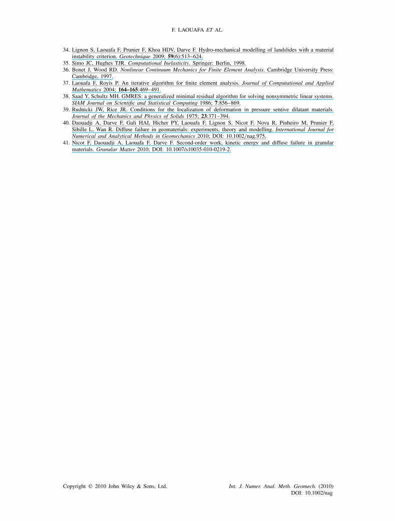
F. LAOUAFA ET AL.

34. Lignon S, Laouafa F, Prunier F, Khoa HDV, Darve F. Hydro-mechanical modelling of landslides with a materialinstability criterion. Geotechnique 2009; 59(6):513–624.

35. Simo JC, Hughes TJR. Computational Inelasticity. Springer: Berlin, 1998.36. Bonet J, Wood RD. Nonlinear Continuum Mechanics for Finite Element Analysis. Cambridge University Press:

Cambridge, 1997.37. Laouafa F, Royis P. An iterative algorithm for finite element analysis. Journal of Computational and Applied

Mathematics 2004; 164–165:469–491.38. Saad Y, Schultz MH. GMRES: a generalized minimal residual algorithm for solving nonsymmetric linear systems.

SIAM Journal on Scientific and Statistical Computing 1986; 7:856–869.39. Rudnicki JW, Rice JR. Conditions for the localization of deformation in pressure sentive dilatant materials.

Journal of the Mechanics and Physics of Solids 1975; 23:371–394.40. Daouadji A, Darve F, Gali HAI, Hicher PY, Laouafa F, Lignon S, Nicot F, Nova R, Pinheiro M, Prunier F,

Sibille L, Wan R. Diffuse failure in geomaterials: experiments, theory and modelling. International Journal forNumerical and Analytical Methods in Geomechanics 2010; DOI: 10.1002/nag.975.

41. Nicot F, Daouadji A, Laouafa F, Darve F. Second-order work, kinetic energy and diffuse failure in granularmaterials. Granular Matter 2010; DOI: 10.1007/s10035-010-0219-2.

Copyright � 2010 John Wiley & Sons, Ltd. Int. J. Numer. Anal. Meth. Geomech. (2010)DOI: 10.1002/nag