Numerical Algorithms for use in a Dynamical Model of the …aja/papers/adcroft_PhD_1995.pdf · Numerical Algorithms for use in a Dynamical Model of the Ocean ... and whose open-mindedness

Numerical Algorithms for use in aDynamical Model of the Ocean

Alistair James Adcroft

A thesis submitted for the degree of

Doctor of PhilosophyUniversity of London

and the

Diploma of Imperial College

1

AbstractA new ocean circulation model based upon the Navier-Stokes equations is presented as a general purpose tool

to study oceanic flows from the small scales of convective processes (∼ 1 km), right through to the scale of theglobal circulation. The horizontal discretisation of the model is based upon the Arakawa ‘C’ grid, but includes a newmethod that overcomes the problem of spurious grid-scale noise that would otherwise be manifest at low resolutions(relative to the Rossby radius of deformation). The model is formulated in terms of finite volumes which allows anaccurate representation of topography to be implemented.

Various classes of wave motion, inherent in the model physics, are derived by linearisation of the governingequations. The distinct wave motions are translated to the context of shallow water theory and analysed. A thoroughunderstanding of how the grid-scale noise behaves in numerical models is developed. Two types of fundamental wavemotion need to be modeled accurately; inertia-gravity waves and Rossby waves. The dispersive properties of thesewaves in a discretised model dictate how grid-scale noise propagates. A new numerical algorithm is then presentedthat evaluates the relevant terms in a more exact manner. The algorithm is shown to accurately model the dispersiveproperties of both inertia-gravity waves and Rossby waves.

Conventional representation of topography, as boxes fitted to the model grid, is severely limited by verticalresolution. The finite volume method, presented here, introduces the concept of zone (volume averaged) quantitiesand flux (area averaged) quantities into which the model variables can be catagorised. The continuous governingequations are then integrated over finite volumes that fit the bottom topography, and are written explicitly in termsof zone and flux quantities. The model is thus able to resolve small variations in bottom relief without explicitlyneeding the equivalent vertical resolution in the interior.

2

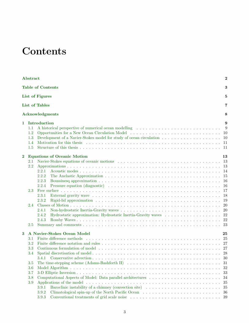
Contents

Abstract 2

Table of Contents 3

List of Figures 5

List of Tables 7

Acknowledgments 8

1 Introduction 91.1 A historical perspective of numerical ocean modelling . . . . . . . . . . . . . . . . . . . . . . . . . . . 91.2 Opportunities for a New Ocean Circulation Model . . . . . . . . . . . . . . . . . . . . . . . . . . . . . 101.3 Development of a Navier-Stokes model for study of ocean circulation . . . . . . . . . . . . . . . . . . . 101.4 Motivation for this thesis . . . . . . . . . . . . . . . . . . . . . . . . . . . . . . . . . . . . . . . . . . . 111.5 Structure of this thesis . . . . . . . . . . . . . . . . . . . . . . . . . . . . . . . . . . . . . . . . . . . . . 11

2 Equations of Oceanic Motion 132.1 Navier-Stokes equations of oceanic motions . . . . . . . . . . . . . . . . . . . . . . . . . . . . . . . . . 132.2 Approximations . . . . . . . . . . . . . . . . . . . . . . . . . . . . . . . . . . . . . . . . . . . . . . . . . 13

2.2.1 Acoustic modes . . . . . . . . . . . . . . . . . . . . . . . . . . . . . . . . . . . . . . . . . . . . . 142.2.2 The Anelastic Approximation . . . . . . . . . . . . . . . . . . . . . . . . . . . . . . . . . . . . . 152.2.3 Boussinesq approximation . . . . . . . . . . . . . . . . . . . . . . . . . . . . . . . . . . . . . . . 162.2.4 Pressure equation (diagnostic) . . . . . . . . . . . . . . . . . . . . . . . . . . . . . . . . . . . . 16

2.3 Free surface . . . . . . . . . . . . . . . . . . . . . . . . . . . . . . . . . . . . . . . . . . . . . . . . . . . 172.3.1 External gravity wave . . . . . . . . . . . . . . . . . . . . . . . . . . . . . . . . . . . . . . . . . 182.3.2 Rigid-lid approximation . . . . . . . . . . . . . . . . . . . . . . . . . . . . . . . . . . . . . . . . 19

2.4 Classes of Motion . . . . . . . . . . . . . . . . . . . . . . . . . . . . . . . . . . . . . . . . . . . . . . . . 202.4.1 Non-hydrostatic Inertia-Gravity waves . . . . . . . . . . . . . . . . . . . . . . . . . . . . . . . . 202.4.2 Hydrostatic approximation: Hydrostatic Inertia-Gravity waves . . . . . . . . . . . . . . . . . . 222.4.3 Rossby Waves . . . . . . . . . . . . . . . . . . . . . . . . . . . . . . . . . . . . . . . . . . . . . . 22

2.5 Summary and comments . . . . . . . . . . . . . . . . . . . . . . . . . . . . . . . . . . . . . . . . . . . . 23

3 A Navier-Stokes Ocean Model 253.1 Finite difference methods . . . . . . . . . . . . . . . . . . . . . . . . . . . . . . . . . . . . . . . . . . . 253.2 Finite difference notation and rules . . . . . . . . . . . . . . . . . . . . . . . . . . . . . . . . . . . . . . 273.3 Continuous formulation of model . . . . . . . . . . . . . . . . . . . . . . . . . . . . . . . . . . . . . . . 273.4 Spatial discretisation of model . . . . . . . . . . . . . . . . . . . . . . . . . . . . . . . . . . . . . . . . . 28

3.4.1 Conservative advection . . . . . . . . . . . . . . . . . . . . . . . . . . . . . . . . . . . . . . . . . 303.5 The time-stepping scheme (Adams-Bashforth II) . . . . . . . . . . . . . . . . . . . . . . . . . . . . . . 313.6 Model Algorithm . . . . . . . . . . . . . . . . . . . . . . . . . . . . . . . . . . . . . . . . . . . . . . . . 323.7 3-D Elliptic Inversion . . . . . . . . . . . . . . . . . . . . . . . . . . . . . . . . . . . . . . . . . . . . . . 333.8 Computational Aspects of Model: Data parallel architectures . . . . . . . . . . . . . . . . . . . . . . . 343.9 Applications of the model . . . . . . . . . . . . . . . . . . . . . . . . . . . . . . . . . . . . . . . . . . . 35

3.9.1 Baroclinic instability of a chimney (convection site) . . . . . . . . . . . . . . . . . . . . . . . . 353.9.2 Climatological spin-up of the North Pacific Ocean . . . . . . . . . . . . . . . . . . . . . . . . . 363.9.3 Conventional treatments of grid scale noise . . . . . . . . . . . . . . . . . . . . . . . . . . . . . 39

3

4 Numerical Representation of Inertia-Gravity Waves 404.1 Shallow Water Theory . . . . . . . . . . . . . . . . . . . . . . . . . . . . . . . . . . . . . . . . . . . . . 404.2 Inertia-Gravity Waves . . . . . . . . . . . . . . . . . . . . . . . . . . . . . . . . . . . . . . . . . . . . . 434.3 Damped wave motion . . . . . . . . . . . . . . . . . . . . . . . . . . . . . . . . . . . . . . . . . . . . . 434.4 Finite-differenced Inertia-gravity waves . . . . . . . . . . . . . . . . . . . . . . . . . . . . . . . . . . . . 444.5 Numerical Shallow Water models . . . . . . . . . . . . . . . . . . . . . . . . . . . . . . . . . . . . . . . 48

4.5.1 B grid shallow water model . . . . . . . . . . . . . . . . . . . . . . . . . . . . . . . . . . . . . . 484.5.2 C grid shallow water model . . . . . . . . . . . . . . . . . . . . . . . . . . . . . . . . . . . . . . 494.5.3 Shallow water model results . . . . . . . . . . . . . . . . . . . . . . . . . . . . . . . . . . . . . . 49

4.6 The Explicit Oscillator Algorithm . . . . . . . . . . . . . . . . . . . . . . . . . . . . . . . . . . . . . . . 544.6.1 Implicit Coriolis: damping of the Extra Inertial Mode . . . . . . . . . . . . . . . . . . . . . . . 554.6.2 Comparison to the standard models . . . . . . . . . . . . . . . . . . . . . . . . . . . . . . . . . 56

4.7 Summary . . . . . . . . . . . . . . . . . . . . . . . . . . . . . . . . . . . . . . . . . . . . . . . . . . . . 60

5 Numerical Representation of Rossby Waves and the Cd scheme 615.1 Rossby Waves . . . . . . . . . . . . . . . . . . . . . . . . . . . . . . . . . . . . . . . . . . . . . . . . . . 615.2 Finite-differenced Rossby waves . . . . . . . . . . . . . . . . . . . . . . . . . . . . . . . . . . . . . . . . 625.3 Time staggered grids . . . . . . . . . . . . . . . . . . . . . . . . . . . . . . . . . . . . . . . . . . . . . . 645.4 The Cd grid scheme: the CD hybrid . . . . . . . . . . . . . . . . . . . . . . . . . . . . . . . . . . . . . 675.5 Determining the optimal coupling . . . . . . . . . . . . . . . . . . . . . . . . . . . . . . . . . . . . . . . 695.6 Shallow water model results . . . . . . . . . . . . . . . . . . . . . . . . . . . . . . . . . . . . . . . . . . 705.7 Implementation of the Cd scheme in the GCM . . . . . . . . . . . . . . . . . . . . . . . . . . . . . . . 765.8 Discussion . . . . . . . . . . . . . . . . . . . . . . . . . . . . . . . . . . . . . . . . . . . . . . . . . . . . 765.9 Summary . . . . . . . . . . . . . . . . . . . . . . . . . . . . . . . . . . . . . . . . . . . . . . . . . . . . 78

6 Representing Topography: the finite volume approach 796.1 Formulations in numerical modeling . . . . . . . . . . . . . . . . . . . . . . . . . . . . . . . . . . . . . 806.2 Finite volume method . . . . . . . . . . . . . . . . . . . . . . . . . . . . . . . . . . . . . . . . . . . . . 81

6.2.1 Continuity equation and boundary conditions . . . . . . . . . . . . . . . . . . . . . . . . . . . . 826.2.2 Tracers . . . . . . . . . . . . . . . . . . . . . . . . . . . . . . . . . . . . . . . . . . . . . . . . . 826.2.3 Momentum Equations . . . . . . . . . . . . . . . . . . . . . . . . . . . . . . . . . . . . . . . . . 846.2.4 Numerical stability . . . . . . . . . . . . . . . . . . . . . . . . . . . . . . . . . . . . . . . . . . . 876.2.5 Comment on Accuracy . . . . . . . . . . . . . . . . . . . . . . . . . . . . . . . . . . . . . . . . . 88

6.3 Testing the finite volume approach . . . . . . . . . . . . . . . . . . . . . . . . . . . . . . . . . . . . . . 886.3.1 Topographic β . . . . . . . . . . . . . . . . . . . . . . . . . . . . . . . . . . . . . . . . . . . . . 886.3.2 Flow over a Gaussian bump . . . . . . . . . . . . . . . . . . . . . . . . . . . . . . . . . . . . . . 92

6.4 Conclusions . . . . . . . . . . . . . . . . . . . . . . . . . . . . . . . . . . . . . . . . . . . . . . . . . . . 101

7 Concluding remarks 1027.1 The Cd scheme . . . . . . . . . . . . . . . . . . . . . . . . . . . . . . . . . . . . . . . . . . . . . . . . . 1037.2 Shaved cells . . . . . . . . . . . . . . . . . . . . . . . . . . . . . . . . . . . . . . . . . . . . . . . . . . . 1037.3 Future development of model . . . . . . . . . . . . . . . . . . . . . . . . . . . . . . . . . . . . . . . . . 1047.4 Future directions in ocean modelling . . . . . . . . . . . . . . . . . . . . . . . . . . . . . . . . . . . . . 104

A Derivation of the Navier-Stokes Equations of Oceanic Motion 106A.1 Conservation of Mass . . . . . . . . . . . . . . . . . . . . . . . . . . . . . . . . . . . . . . . . . . . . . . 106A.2 Conservation of momentum . . . . . . . . . . . . . . . . . . . . . . . . . . . . . . . . . . . . . . . . . . 107A.3 Conservation of salt . . . . . . . . . . . . . . . . . . . . . . . . . . . . . . . . . . . . . . . . . . . . . . 108A.4 Thermodynamics (Continuity of heat, conservation of energy and potential temperature) . . . . . . . . 108A.5 Pressure equation (prognostic) . . . . . . . . . . . . . . . . . . . . . . . . . . . . . . . . . . . . . . . . 110

B Scaling of non-hydrostatic effects 111

C Solution for zonal flow over a Gaussian bump 113

Bibliography 115

4

List of Figures

2.1 Schematic of the single layer shallow water model . . . . . . . . . . . . . . . . . . . . . . . . . . . . . . 18

3.1 Describing f(x) with discrete variables fi . . . . . . . . . . . . . . . . . . . . . . . . . . . . . . . . . . 263.2 Three-dimensional ‘C’ grid . . . . . . . . . . . . . . . . . . . . . . . . . . . . . . . . . . . . . . . . . . . 293.3 Flow diagram for the pre-conditioned conjugate gradient algorithm . . . . . . . . . . . . . . . . . . . . 343.4 Decomposition of ocean domain . . . . . . . . . . . . . . . . . . . . . . . . . . . . . . . . . . . . . . . . 343.5 Density anomaly at z=-250m at day 10 in a convection experiment . . . . . . . . . . . . . . . . . . . . 353.6 Pressure (in m) at z=-12.5 m at end of year 43. . . . . . . . . . . . . . . . . . . . . . . . . . . . . . . . 373.7 Temperature (in oC) at λ=171.5E at end of year 43. . . . . . . . . . . . . . . . . . . . . . . . . . . . . 373.8 Salinity (in psu) at λ=171.5E at end of year 43. . . . . . . . . . . . . . . . . . . . . . . . . . . . . . . . 373.9 Vertical velocity at the base of the top layer after one month . . . . . . . . . . . . . . . . . . . . . . . 383.10 Vertical velocity at z=-3200m in the model after one month . . . . . . . . . . . . . . . . . . . . . . . . 38

4.1 Schematic of the two layer shallow water model . . . . . . . . . . . . . . . . . . . . . . . . . . . . . . . 414.2 Arakawa grids A-E . . . . . . . . . . . . . . . . . . . . . . . . . . . . . . . . . . . . . . . . . . . . . . . 444.3 Non-dimensional frequency of inertia-gravity waves . . . . . . . . . . . . . . . . . . . . . . . . . . . . . 464.4 Non-dimensional frequency of discrete inertia-gravity waves at high resolution . . . . . . . . . . . . . . 464.5 Non-dimensional frequency of discrete inertia-gravity waves at low resolution . . . . . . . . . . . . . . 474.6 Low resolution (4S/∆x2 = 1/5) integrations of the B grid (left) and C grid (right) shallow water models 504.7 Low resolution (4S/∆x2 = 1/5) integrations of the B grid (left) and C grid (right) shallow water models 514.8 High resolution (4S/∆x2 = 5) integrations of the B grid (left) and C grid (right) shallow water models 524.9 High resolution (4S/∆x2 = 5) integrations of the B grid (left) and C grid (right) shallow water models 534.10 Low resolution (4S/∆x2 = 1/5) integrations of the explicit oscillator scheme on the C grid . . . . . . . 574.11 High resolution (4S/∆x2 = 5) integrations of the explicit oscillator scheme on the C grid . . . . . . . . 584.12 Explicit Oscillator scheme at high resolution (4S/∆x2 = 1/2) integrations on a β-plane . . . . . . . . 59

5.1 Rossby wave dispersion relations for the continuum and high resolution finite difference models . . . . 645.2 Rossby wave dispersion relations for the continuum and low resolution finite difference models . . . . . 655.3 The Eliassen time horizontally staggered grids, AA’,BB’,CC’,DD’,EE’ . . . . . . . . . . . . . . . . . . 665.4 The single step C grid compared to the time staggered grids DD’ CD . . . . . . . . . . . . . . . . . . . 675.5 The two step Cd grid. . . . . . . . . . . . . . . . . . . . . . . . . . . . . . . . . . . . . . . . . . . . . . 685.6 h, ζ and D for the B, C and Cd models at t = 40 in experiment I . . . . . . . . . . . . . . . . . . . . . 725.7 h, ζ and D for the B, C and Cd models at t = 5000 in experiment I . . . . . . . . . . . . . . . . . . . . 735.8 h, ζ and D for the B, C and Cd models at t = 40 in experiment II . . . . . . . . . . . . . . . . . . . . 745.9 h, ζ and D for the B, C and Cd models at t = 5000 in experiment II . . . . . . . . . . . . . . . . . . . 755.10 Vertical velocity at the base of the top layer in the model after one month . . . . . . . . . . . . . . . . 775.11 Vertical velocity at z=-3200m in the model after one month . . . . . . . . . . . . . . . . . . . . . . . . 77

6.1 Four methods of representing topography in numerical models . . . . . . . . . . . . . . . . . . . . . . . 806.2 A schematic of a shaved cell . . . . . . . . . . . . . . . . . . . . . . . . . . . . . . . . . . . . . . . . . . 816.3 Centres of volumes for shaved cells . . . . . . . . . . . . . . . . . . . . . . . . . . . . . . . . . . . . . . 846.4 Pressure and velocity vectors at t = 1 yr for the flat bottomed β-plane integration. . . . . . . . . . . . 906.5 Pressure and velocity vectors at t = 1 yr for the sloping bottom f-plane integration. . . . . . . . . . . 916.6 Schematic flow over an isolated topographic feature. . . . . . . . . . . . . . . . . . . . . . . . . . . . . 926.7 Barotropic stream function at day 60 with constant zonal flow removed. . . . . . . . . . . . . . . . . . 936.8 Barotropic stream function at day 60 with analytic solution removed. . . . . . . . . . . . . . . . . . . 936.9 Barotropic stream function Ψ from the SPEM integration . . . . . . . . . . . . . . . . . . . . . . . . . 95

5

6.10 Barotropic stream function Ψ from the shaved cell integration . . . . . . . . . . . . . . . . . . . . . . . 956.11 Depth Integrated Relative Vorticity in the SPEM integration . . . . . . . . . . . . . . . . . . . . . . . 966.12 Depth Integrated Relative Vorticity in the shaved cell integration . . . . . . . . . . . . . . . . . . . . . 966.13 Density anomaly at z = −4000 m in the SPEM integration . . . . . . . . . . . . . . . . . . . . . . . . 976.14 Potential Temperatures at z = −4219 m in the shaved cell integration . . . . . . . . . . . . . . . . . . 976.15 Schematic of Gaussian bump represented by “step-topography” and “shaved-cells” . . . . . . . . . . . 986.16 Potential temperature at z=-3656 m and t=1 day using the step-wise representation of topography. . . 1006.17 Potential temperature at z=-3656 m and t=1 day using the shaved cell representation of topography. . 100

6

List of Tables

3.1 GCM mixing and diffusion coefficients for the North Pacific spin-up . . . . . . . . . . . . . . . . . . . 36

4.1 External parameters used in the comparison of the B and C grid shallow water models . . . . . . . . . 49

5.1 Parameters for the double gyre integrations of the B grid, C grid and Cd models. . . . . . . . . . . . . 70

6.1 Parameters for the two experiments to model planetary (I) and topographic (II) β effects. . . . . . . . 896.2 Parameters for the the comparison experiment to SPEM . . . . . . . . . . . . . . . . . . . . . . . . . . 94

7

Acknowledgments

I take this opportunity to thank my supervisor, John Marshall, for the advice he has given me throughout thelast few years, and especially for the direction and opportunities he has given me by involving me in the modeldevelopment.

I also wish to thank the other members of the development team; Chris Hill, Curtis Heisey and Lev Perelman. Iespecially thank Chris without whose attention to detail and organisation, the model would not have come as far asit has, and whose open-mindedness allowed me to try out many schemes in the model. I only wish more of them hadworked. Thanks also to Dimitri Menemenlis for proof reading and for allowing me full reign over the chalk board.

I thank Paul Cloke who inadvertently interested me in the “gridding” issue and who, in the early days, schooledme in the art of numerical methods.

I am grateful to the Natural Environment Research Council for providing a studentship, to the Space andAtmospheric Physics group of Imperial College and to the faculty and staff of the Center for Meteorology andPhysical Oceanography at MIT for hosting me in the recent years.

I would like to thank my examiners, Dr. Dan Moore and Dr. David Webb for their comments on an earlierrevision of the text, and for their willingness to examine this thesis at such short notice.

And finally, I thank my fiancee, Sonya Legg, for her support, especially on those days when all seemed lost.

8

Chapter 1

Introduction

1.1 A historical perspective of numerical ocean modelling

To understand the ocean circulation and the role of the ocean in the climate system, we must understand complexprocesses in the ocean that occur on a wide range of scales. We use numerical models as tools for furthering ourunderstanding of both the large scale circulation and small scale processes. The large scale circulation is intimatelylinked with processes on smaller scales. These processes must be either resolved or accurately parameterised if weare to render an accurate picture of the global ocean. The scale of geostrophic turbulence in the ocean is of the order30–100 km which is very much smaller than the typical 1000 km scale in the atmosphere. The limitations on spatialresolution of numerical models, imposed by computer technology, are therefore more severe for ocean modelling thanfor meteorology.

Since the earliest attempts to use computers to help understand the ocean circulation computers have becomeever more powerful. The computers accessible by most oceanographers today are orders of magnitude faster, and canstore much more data, than those available in the 1960’s when the first real efforts to model the ocean were beingmade. The earliest attempts to model the global scale circulation could not possibly resolve the meso-scale featurespresent in the ocean. Instead, these processes had to be parameterised and, indeed, this is still the norm in regionaland global calculations.

The first large scale ocean simulation was carried out by Sarkisyan [Sar55] in the mid ’50s. Subsequent work bySarkisyan focused on regional studies such as for the North Atlantic. Bryan began modelling the ocean at GFDLby applying numerical methods to the solution of the barotropic vorticity equation [Bry63] in the early ’60s. Later,ocean modelling started elsewhere with Friedrich constructing a multi-level model in West Germany [Mos66]. Bryan,in the meantime, moved onto three-dimensional box models and started a number of multi-level primitive equationstudies with Cox [BC68]. Soon after, a more general model was developed that incorporated irregular coast-lines andvariable bottom topography [Bry69]. The methods laid out by Bryan and Cox have been the foundation of manysubsequent modelling efforts by other parties.

The limitations imposed by the state of the computer technology meant that the Cox and Bryan model was firstapplied to regional simulations. These included regional simulations of the Southern, Indian and North AtlanticOceans. Another model was then being developed in parallel at UCLA by Haney, Arakawa and Takano [Han71].Takano went on to develop a less general model but applied it to the global ocean. He applied idealized atmosphericforcing and obtained an ocean circulation with many realistic features [Tak74, Tak75].

Since then, several multi-level primitive equation models have been developed. Semtners code [Sem74] is aderivative of the Bryan and Takano models. Two attempts to formulate the model on an Arakawa C grid, followingthe UCLA Atmospheric GCM were made. Jeong-Woo Kim [Kim79] and Cox (unpublished) found the models to besusceptible to grid-scale noise and they are apparently no longer in use [Jr.86]. Nevertheless, atmospheric modelswere being successfully built on C grids since they resolved the geostrophic adjustment process1. Ocean models wereconstructed on the B grid since they were unable to resolve the Rossby radius of deformation which is much smallerin the ocean than in the atmosphere.

Further adaptions of the Bryan formulation were made by Han [Han84] and Cox [Cox84] and now, in the mid1990’s, there are many models derived from or based on this formulation. Recent development of the Bryan-Cox-Semtner code has been carried out at Los Alamos by Dukowicz and Smith [DSM93, DS94]. They have moved froma stream function approach for treating the barotropic mode to a surface pressure approach. This allows islands to

1The inherent strengths and weaknesses of the B and C grid formulations as a function of resolution is described in detail in chapter4.

9

be treated more appropriately.All these models use height as the vertical co-ordinate. More recent models have departed from this convention.

MICOM, developed by Smith and Bleck [SBB90], is an isopycnal model where height is a prognostic variable andpotential density is the vertical co-ordinate. The advantage of isopycnal co-ordinates is that the parameterizationof sub-grid scale processes can be made adiabatic. The formulation does however introduce complications bothat the solid boundaries and at the surface, and has difficulties when incorporating an accurate equation of state.SPEM, see Haidvogel et al., 1991 [HWY91], and the Princeton model, see Mellor 1992 [Mel92], use terrain followingσ co-ordinates. These models are well suited for coastal oceanography where high horizontal resolution allows σco-ordinates to follow the topography smoothly. The SPEM code has not been widely applied at global scalespresumably because the topography of the ocean is extremely irregular and has many islands. The Princeton modeluses a variant of σ co-ordinates where the number of modes in the vertical can be varied in the horizontal to allowsudden changes in topography.

1.2 Opportunities for a New Ocean Circulation Model

The advent of new parallel computer architectures has recently allowed oceanographers to begin running models ateddy resolving resolutions on a global scale (see, for example Semtner, 1988 [SC88]). As the available memory ofcomputers increases, issues involving grid resolution must be re-addressed. One such issue concerns the approxima-tions made to the governing equations used for large scale ocean modelling. For example, the usual approximationof hydrostatic balance in the vertical may not be strictly valid at the smaller scales (smaller than the Rossby de-formation radius) now being resolved by these models. Further, horizontal Coriolis effects can only be investigatedif the hydrostatic approximation is relaxed. Small scale phenomena are interesting in their own right and can onlybe investigated using a non-hydrostatic model. Currently, all global ocean models are hydrostatic and there has notbeen, until now, a numerical model applicable to both the small and the large scale. Such a model would allow asmooth transition between studies at high and low resolution.

Models which resolve the Rossby radius of deformation operate in a parameter regime analogous to that of mostatmospheric models. They do not, therefore, suffer from the excessive grid scale noise, confronted independently byKim and by Cox.

Just as advances in computers allow the global circulation models to increase their resolution, the same advancespermit models designed primarily for the study of small scale phenomena to be applied to the larger scale.

Here, one such model is described that is applicable to all scales in the ocean. It has successfully been appliedto the convective overturning scale, up through the meso-scale and in extended integrations at the global scale. Themodel is non-hydrostatic, though it can operate in a hydrostatic or quasi-hydrostatic mode. It is formulated on a Cgrid, but uses an innovative method for evaluating the Coriolis term so that it is not susceptible to the grid-scalenoise problems of C grid models.

1.3 Development of a Navier-Stokes model for study of ocean circula-

tion

The model described here uses height as a vertical co-ordinate and can have arbitrary topography and irregular coast-lines (or may be periodic in x and/or y). The kernel of the model is founded on the incompressible Navier-Stokesequations. It can also be used to step forward quasi-hydrostatic and hydrostatic models that employ approximatedforms of the governing equations.

The model incorporates ideas developed in the computational fluid dynamics community which are relatively newto ocean modelling (eg. conjugate gradient methods and finite volume methods). It has been developed on a parallelcomputer architecture that gives the modeller access to higher resolution, through increased memory, and to longerintegrations, through increased speed.

The model solves the incompressible Navier-Stokes equations and so involves fewer assumptions than the hy-drostatic primitive equations employed in most existing models. Further approximated forms can be recovered bymeans of “switches” so that the relative importance of various small terms can be evaluated. In particular, thenon-hydrostatic facility can be turned on or off selectively; a quasi-hydrostatic form of the model allows horizontalCoriolis effects to be retained whilst neglecting the advection of vertical momentum.

The Navier-Stokes model has been designed for the study of dynamical processes in the ocean ranging from theconvective scale, through the geostrophic eddy scale to the global scale circulation. The algorithm for studying

10

this wide range of scales is essentially the same, though approximations2 can be made at larger scales to make theintegration more efficient with no significant loss of accuracy.

The computational challenge is to maintain non-divergence of the flow. This entails diagnosing the appropriatepressure field that ensures the flow has zero divergence at all times. The equation satisfied by the pressure field iselliptic and has Neumann boundary conditions. Thus, the pressure field depends upon the global distribution ofinhomogeneous sources and boundary conditions.

This last aspect of the problem has implications for implementation on parallel computers. Global interaction,required by the elliptic problem, demands that information be exchanged globally between processors on a parallelmachine. The reduction of inter-processor communication is thus a priority in designing such an algorithm.

The development of the model has required expertise from diverse fields. Knowledge of ocean physics, numericalmethods, parallel computer architectures, data management and visualisation were supplied by members of a largeteam; nominally John Marshall, Chris Hill, Lev Perelman, Curtis Heisey, and myself. Discussions with Prof. Arvind,Andrew White, Roger Brugge, and Paul Cloke, among others, helped guide the development of the model.

1.4 Motivation for this thesis

The model is developed on a ‘C’ grid because it is the appropriate grid for study of small scale phenomena. It is alsothe natural grid for both a finite volume formulation and the pressure correction method. When applied at coarseresolution, the pure ‘C‘ grid model is found to be susceptible to grid-scale noise, as was the case for Kim and for Cox.This is a direct consequence of the choice of gridding and is a well documented problem, most notably by Arakawaand Lamb [AL77]. To evaluate the Coriolis term on the C grid, the horizontal velocities must be spatially averaged.A result of the spatial averaging is that the Coriolis term vanishes for the grid scale. Grid scale noise can thereforeexist as stationary waves that have no inertial oscillatory component. For this reason, low resolution ocean modelsare formulated on other grids, typically the Arakawa B grid.

This thesis has two foci. The first concerns the representation of the Coriolis term on a staggered grid, or,more generally, on the representation of inertia-gravity and Rossby waves in numerical models. Noise, manifest inthe ‘w’ field, was resilient to many attempts to control it. Many approaches, ranging from brute-force filtering tothe introduction of artificial damping terms, were attempted. None of these methods were satisfactory for variousreasons. We decided, therefore, to find a correction to the problem rather than try to control it. This led to theformulation of what we term the Cd scheme; a D grid is used in tandem with the C grid where the D grid velocitiesare used to evaluate the Coriolis term. The scheme can be successfully used at coarse resolution and avoids the gridscale noise problems that would otherwise manifest themselves.

The second issue addressed in this thesis is the representation of topography. The conventional representationof topography in height co-ordinate models is as “step-wise” functions fitted to the model layer depths, a cruderepresentation. As an alternative, we consider a finite volume approach in which shaved cells can be used to representtopography. The ‘C’ grid formulation lends itself quite naturally to a finite volume interpretation of the model. Thefinite volume approach aims to conserve properties such as volume and tracers in a precise manner. The modelequations are discretised by integrating them over a grid of finite volumes. In the interior, the use of regular volumesor cells gives rise to a conventional discretisation. However, the cells need not be regular where they abut a solidboundary. We take advantage of this by shaving the cells to fit the topography of the ocean. In this manner, themodel is able to represent topographic effects that could otherwise not be represented without prohibitive increasesin horizontal and vertical resolution.

1.5 Structure of this thesis

Chapter 2 presents the continuous equations of motion on which the model is based. The approximations implicit inthe Navier-Stokes equations are discussed. Finally the natural modes of motion at various degrees of approximationare derived. Subsequent chapters concern the accurate representation of these motions in numerical models.

The kernel of the numerical model, excluding the implementation of the two innovations, is described in chapter3. Here, the model is integrated in a realistic configuration and found to be susceptible to grid-scale noise whenthe Rossby radius of deformation is not resolved. The nature of the noise is traced to the spatial averaging of theCoriolis term on a C grid. Several attempts to control the noise problem are briefly outlined and discussed.

Chapters 4 and 5 deal with the issue of the spatially averaged Coriolis term on a C grid. The similarity betweenthe shallow water equations of motion and the equations pertaining to a baroclinic mode in the Navier-Stokes model

2The hydrostatic approximation is described at the end of chapter 2.

11

is used to motivate a study of the gridding issue in the context of the shallow water equations. Chapter 4 reviewsthe work of Arakawa and Lamb [AL77] and describes a scheme that improves the representation of inertia-gravitywaves. The scheme is flawed due its inability to represent Rossby waves. A new scheme, the Cd scheme, is thendescribed in chapter 5, which correctly treats both inertia-gravity waves and Rossby waves.

The Cd scheme is implemented in a numerical shallow water model and compared with the B and C grids. Itis found to have no grid scale noise problems and is subsequently implemented in the Navier-Stokes model. Thescheme entails only minor modification of the original model (as described in chapter 3) and adds little computationaloverhead.

In chapter 6, the representation of topography is discussed. The finite volume approach and the use of shavedcells to represent topography are described. The model is re-formulated using finite volumes. A series of experimentsare devised and conducted to test the representation of topography using shaved cells.

12

Chapter 2

Equations of Oceanic Motion

All classes and scales of motion are described by the Navier-Stokes equations (derived in Appendix A). The equationsused for the study of the general circulation of the ocean, however, are based on approximated forms which involvethe Boussinesq approximation and assume non-divergence of the flow. The latter approximation excludes the acousticmodes of motion.

Further degrees of approximation are made that modify but do not eliminate the remaining natural modes ofmotion. These classes of motion will be derived. The accurate representation of these modes was a paramountconcern when building and understanding the finite difference model. Chapters 4 and 5 deal exclusively with thenumerical representation of inertia-gravity waves and Rossby waves, the nature of which will be derived at the endof this chapter.

2.1 Navier-Stokes equations of oceanic motions

The complete unapproximated system that describes inviscid, adiabatic flow is:

Dp

Dt+ ρc2s∇.u = 0 (2.1a)

Du

Dt+ 2Ω ∧ u +

∇p

ρ+ ∇Φ = 0 (2.1b)

DS

Dt= 0 (2.1c)

Dθ

Dt= 0 (2.1d)

ρ = ρ(θ, S, p) (2.1e)

where p, u = [u, v, w], θ, S and ρ are the pressure, three-dimensional velocity, potential temperature, salinity andin-situ density respectively. These equations are derived in Appendix A from first principles.

There are six prognostic equations for the variables p, u, θ and S and one diagnostic relation for ρ. These arethe Navier-Stokes equations supplemented by complete thermodynamics. These equations are the basis from whichall models of the ocean are derived in their various degrees of approximation.

The full system is often also expressed in terms of in-situ temperature T rather than potential temperature θ.Similarly, the salt and temperature equations can be combined into a thermodynamic equation for potential densitydefined σpo

= ρ(θ, S, po) ⇒ ddtσpo

= 0.The pressure equation will later reduce to the continuity equation (expressing non-divergence of the flow) when

the acoustic modes have been filtered out of the system. The pressure equation is obtained by combining conservationof mass with the equation of state. The Navier-Stokes equations could equally have been written using conservationof mass instead of the pressure equation. This, however, would have yielded two explicit equations for the density,ρ, and none for the pressure, p.

2.2 Approximations

System 2.1 is completely general and describes all physical processes in the ocean that are not affected by molecularviscosity and diffusivity. This, however, is a draw back for any practical computation since the explicit time scales

13

in the system require that all processes be resolved. For example, the acoustic modes are very fast relative to anyprocess relevant to the long time scales of interest (normally much longer than a few days). An explicit numericalmodel based on the above system would have a time step limited by the sound waves. This severely limits theapplicability of any such numerical model.

There are two ways of proceeding; either writing the numerical model in an implicit manner or explicitly filteringout the fast modes. Implicit models can be written, and in fact would bear a striking resemblance to the adjusted orfiltered model. Implicit techniques act to slow the respective process down so that a long time step does not violateany criteria. The filtered system, in the other limit, assumes that the process acts infinitely fast so that the systemis always adjusted. The latter approach is more common because it is considerably easier to implement.

Three types of approximation will be used throughout the rest of this chapter:

Rapid time scale approximation in which the mode under consideration is considered much faster than thetime scales of interest. Filtering of these modes assumes that the process has acted infinitely fast and that thefluid is instantaneously adjusted. The acoustic modes and surface gravity waves will be filtered in this manner.

Short spatial scale approximation in which the spatial scale of a mode is very much shorter than any scale ofinterest. For instance, internal inertia-gravity waves behave in a hydrostatic manner except where the aspectratio of the motion is small.

Small amplitude approximation in which the amplitude of an effect is much smaller than the signals of interest.For example, the amplitude of density perturbations due to the transit of an acoustic wave are typically muchsmaller than the dynamically interesting variations arising from mean vertical motion excursions.

These classifications are not exclusive and often one is implied by another.In the account that follows, classes of motion will be derived and approximations made that either modify or

filter the modes of motion.

2.2.1 Acoustic modes

To derive the acoustic modes of motion, consider a reduced form of the Navier-Stokes equations; the conservation ofmass, momentum equations retaining just the local acceleration and pressure gradient terms and equation of state(the dependence on temperature and salinity can be neglected for adiabatic motion):

∂

∂tu +

1

ρ∇p = 0 (2.2a)

∂

∂tρ+ ∇ · (ρu) = 0 (2.2b)

ρ = ρ(p) (2.2c)

Combining the conservation of mass and the reduced equation of state gives the pressure equation. Linearizingabout some mean state then yields:

∂

∂tu +

1

ρo∇p = 0

∂

∂tp+ ρoc

2s∇ · u = 0

The three dimensional divergence of the momentum equations is:

∂

∂t∇.u +

1

ρo∇

2p (2.3)

This can be substituted into the time derivative of the pressure equation to yield:

∂2

∂t2p = c2s∇

2p (2.4)

which is a non-dispersive wave equation describing waves with phase and group speed cs. The speed of sound inwater is approximately 1500 ms−1

The acoustic modes act to adjust the pressure field so that the tendency for the three-dimensional divergence ofthe flow is to vanish. The wave motion would be eliminated if either of the time derivatives in 2.2a and 2.2b wereremoved, or if the pressure dependence of density were removed. Setting ∂ρ

∂p

∣

∣

∣

θ,S→ 0 means that the speed of sound

becomes infinite, cs → ∞.

14

2.2.2 The Anelastic Approximation

As mentioned earlier, filtering out of the sound waves can be achieved by assuming the limiting case of incom-pressibility that makes the sound speed become infinite, cs → ∞. An intermediate approximation, the anelasticapproximation, that retains compressibility effects requires a reference state (denoted by the subscript r) to bedefined as follows:

∂pr

∂z = −gρr(z)p = pr(z) + p′ ρ = ρr(z) + ρ′

(2.5)

where both ρr and pr are prescribed functions of the vertical co-ordinate. Deviations from the reference state aredenoted by primes. The momentum equation is unapproximated.

∂

∂tρu + ∇ · (ρuu) + 2Ω ∧ ρu + ∇p′ + ρ′∇Φ (2.6)

The pressure equation becomes:DprDt

+Dp′

Dt= −ρc2s∇.u (2.7)

The anelastic approximation can be obtained by assuming that the perturbations in the pressure field propagate

so fast that the pressure field is always adjusted. This means that Dp′

Dt Dpr

Dt is a good approximation for the slow

and long scales of interest. Noting that Dpr

Dt = w ∂pr

∂z , the pressure equation can be approximated:

∇.u =gρrc2sρ

w (2.8)

This assumption only deals with time scales and so the equation of state still has a dependence on p′. This isinconsistent with the continuity equation because there would then be two different prognostic equations for density.Therefore, a more consistent method is to, instead, make an assumption about the amplitudes of motion.

Assume that the amplitudes of motion are such that density changes induced by the acoustic pressure pertur-bations are very much smaller than the density changes brought about by large changes in depth (i.e. ∂ρ

∂p′ ∂ρ∂pr

).Then the equation of state becomes:

ρ = ρ(θ, S, pr) (2.9)

Differentiating this equation and making use of the continuity equation, the same anelastic continuity equationis derived. In this manner, the equation of state is consistent with the approximated pressure equation.

The complete anelastic system is then:

∇.u =gρrc2sρ

w (2.10a)

Du

Dt+ 2Ω ∧ u +

∇p′

ρ+ρ′

ρ∇Φ = 0 (2.10b)

DS

Dt= 0 (2.10c)

Dθ

Dt= 0 (2.10d)

ρ = ρ(θ, S, pr) (2.10e)

It should be pointed out that there is no explicit equation for the pressure field p′. A diagnostic equation for p′

can be deduced by combining the momentum equations with the anelastic continuity equation to form an ellipticequation. This will be done later.

The system no longer contains sound waves but does still contain the effects of compressibility brought about bythe slow motions that involve changes in depth.

The removal of the acoustic modes reduces the number of natural modes to four. The appropriate number ofprognostic equations is obtained by replacing the w equation with the anelastic equation so that there are threediagnostic equations; an elliptic equation for pressure, the anelastic equation and the equation of state.

15

2.2.3 Boussinesq approximation

The name Boussinesq approximation is not always used in a consistent fashion. In fact it refers to a wide range ofvery different degrees of approximation from anelastic flow, through non-divergent yet compressible flow, to fullyincompressible flow. Two steps will be described here; the first makes use of an observation about the significanceof density perturbations, the second notes that the scale height over which compressibility effects are important isvery much greater than the real depth of the ocean.

In the ocean, variations in density are small compared to a typical mean value, ρ′/ρo ≈ 10−3. Thus, whereverthe full density is used, it can be approximated by the mean value ρo. This is a trivial exercise when applied tothe anelastic equations above. If the exercise is applied to the Navier-Stokes equations, special care is needed whenconsidering the gravitational term. By taking out the reference pressure (now defined ∂

∂zpr = −gρr = −gρo so thatsimply pr = −gρoz), the gravitational term is naturally handled.

The second step notes, that in the anelastic continuity equation, the two terms involving w are ∂w∂z and g

c2sw. The

scaling of these two terms goes like 1H and g

c2s. The exponential scale depth

c2sg ≈ 225 km is around 50 times larger

than the deeper parts of the real ocean. Thus the anelastic term is typically quite small and can be neglected leavingthe non-divergence condition.

The Boussinesq equations of motion for non-divergent yet compressible flow are:

∇.u = 0 (2.11a)

Du

Dt+ 2Ω ∧ u +

∇p′

ρo+ρ′

ρo∇Φ = 0 (2.11b)

DS

Dt= 0 (2.11c)

Dθ

Dt= 0 (2.11d)

ρ = ρ(θ, S,−gρoz) (2.11e)

Note that the Lagragian form of the equations is readily interchanged with the Eulerian or flux divergence frombecause of the non-divergence of the flow; ∂

∂tφ + ∇ · (φu) = DφDt . This is useful when formulating finite difference

models since conservation is better expressed as the divergence of a flux.There is now apparently an inconsistency between the equation of state which admits compressible effects and

the statement of the non-divergent flow. Taking the time derivative of the equation of state:

dρ

dt=

1

c2s

dprdt

=−gρoc2s

w (2.12)

If the continuity equation is still satisfied then the non-divergence of the flow would be violated:

c2s∇.u = −gw (2.13)

Therefore, the Boussinesq approximation must relax the principle of conservation of mass and instead replace thisprinciple with the non-divergence condition. This equation is usually termed the incompressibility condition thoughthis is misleading since the compressible effects felt through the dependence of temperature and density on depth arestill incorporated. The incompressibility condition expresses a constancy of volume and is thus a pivotal equationfor the formulation of a model built around fixed, finite volumes. Conservation of total mass has therefore beenexchanged for constant total volume.

2.2.4 Pressure equation (diagnostic)

As mentioned earlier for the anelastic equations, there is no prognostic equation for the pressure in the Boussinesqequations, as written above. A prognostic equation for p′ can be found by combining the incompressibility conditionwith the momentum equations. For convenience, first define the vector G to be all the terms of the momentumequations except the local derivative and pressure gradient:

G ≡ −(u.∇)u − 2Ω ∧ u− ρ′

ρo∇Φ (2.14)

16

Now the momentum equations can be written simply:

∂u

∂t+

1

ρo∇p′ = G (2.15)

The flow must be non-divergent for all time. Substituting the momentum equations into the incompressibilitycondition yields:

1

ρo∇

2p′ = ∇.G − ∂

∂t∇.u (2.16)

where the last term should vanish. In practice, the last term is kept to stabilise the numerical model so that anydivergence of the flow is seen by the pressure field and adjusted for.

The final form for the Boussinesq equations is:

∇2p′ = ρo∇.G (2.17a)

∂uh∂t

= Gh −1

ρo∇hp

′ (2.17b)

∂w

∂z= −∇h.uh (2.17c)

Dt

Dtθ = 0 (2.17d)

Dt

DtS = 0 (2.17e)

ρ = ρ(θ, S,−gρoz) (2.17f)

G = −(u.∇)u − 2Ω ∧ u− ρ′

ρo∇Φ (2.17g)

The boundary conditions for the elliptic problem take the form of a Neumann condition on the normal gradientat the boundaries. The exact details pertaining to solid boundaries will be left until the numerical sections. Theboundary condition applied at the free-surface is one of continuity of pressure across the interface, i.e. ocean surfacepressure and atmospheric surface pressure will be the same.

2.3 Free surface

The surface of the ocean is free to move in response to the net accumulation of depth integrated mass fluxes andto mass fluxes across the interface (precipitation, evaporation, river discharge, freezing and thawing). The lattersources are normally grouped into the thermodynamics of the model. In the incompressible model, the mass flux isreplaced by a volume flux, or, in other words, the continuity equation becomes the incompressibility condition. Theequation of evolution for the free surface, ignoring sources and sinks of mass, can be obtained by considering theincompressibility condition, integrated over the total depth of the ocean:

h(x,y,t)∫

−H(x,y)

(∇h · uh +∂w

∂z) dz =

h(x,y,t)∫

−H(x,y)

∇h · uh dz + [w(z)]h(x,y,t)−H(x,y) = 0 (2.18)

where z = −H(x, y) defines the solid ocean bottom and z = h(x, y, t) defines the position of the air-sea interface.The Leibniz formula connects the depth integral of the horizontal divergence to the horizontal divergence of thebarotropic flow:

∇h ·h(x,y,t)∫

−H(x,y)

uh dz =

h(x,y,t)∫

−H(x,y)

∇h · uh dz + (uh(z = h) · ∇h− uh(z = −H) · ∇(−H)) (2.19)

The kinematic boundary condition applicable at both interfaces is that a particle on the interface will remain onthe interface; DtDtzboundary

= w. Applied to the free surface and bottom:

Free surface:Dt

Dth− wh =

∂h

∂t+ uh(z = h) · ∇h− wh = 0 (2.20)

17

(x,y)

z

h

HoH(x,y)

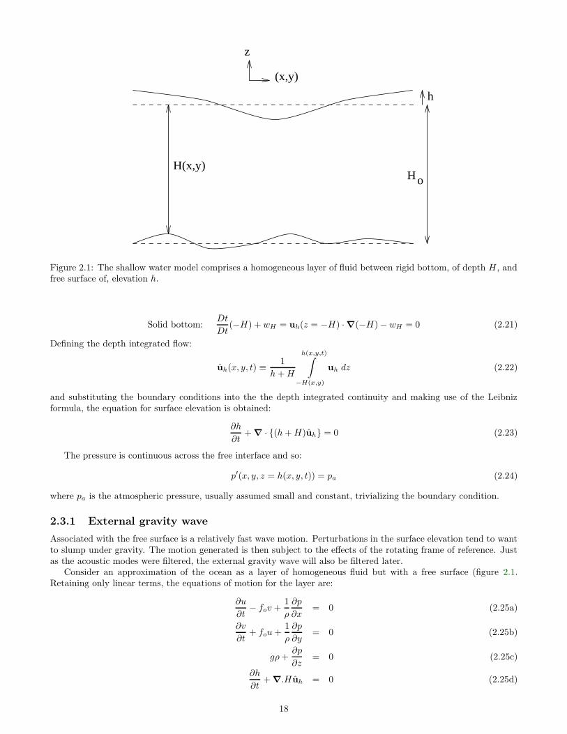
Figure 2.1: The shallow water model comprises a homogeneous layer of fluid between rigid bottom, of depth H , andfree surface of, elevation h.

Solid bottom:Dt

Dt(−H) + wH = uh(z = −H) · ∇(−H) − wH = 0 (2.21)

Defining the depth integrated flow:

uh(x, y, t) ≡1

h+H

h(x,y,t)∫

−H(x,y)

uh dz (2.22)

and substituting the boundary conditions into the the depth integrated continuity and making use of the Leibnizformula, the equation for surface elevation is obtained:

∂h

∂t+ ∇ · (h+H)uh = 0 (2.23)

The pressure is continuous across the free interface and so:

p′(x, y, z = h(x, y, t)) = pa (2.24)

where pa is the atmospheric pressure, usually assumed small and constant, trivializing the boundary condition.

2.3.1 External gravity wave

Associated with the free surface is a relatively fast wave motion. Perturbations in the surface elevation tend to wantto slump under gravity. The motion generated is then subject to the effects of the rotating frame of reference. Justas the acoustic modes were filtered, the external gravity wave will also be filtered later.

Consider an approximation of the ocean as a layer of homogeneous fluid but with a free surface (figure 2.1.Retaining only linear terms, the equations of motion for the layer are:

∂u

∂t− fov +

1

ρ

∂p

∂x= 0 (2.25a)

∂v

∂t+ fou+

1

ρ

∂p

∂y= 0 (2.25b)

gρ+∂p

∂z= 0 (2.25c)

∂h

∂t+ ∇.Huh = 0 (2.25d)

18

Integrating the hydrostatic balance, the homogeneity of the layer dictates that the horizontal pressure gradientsbe independent of depth:

p(x, y, z) = gρ(h− z) + p|z=h (2.26)

⇒ ∇hp = gρ∇hh (2.27)

where the horizontal variations in atmospheric pressure have been neglected. The horizontal flow, uh, is then easilyapproximated as being barotropic also (a consequence of the Taylor-Proudman theorem).

For the flat bottom case (H is constant), linear barotropic equations can be written exclusively in terms of thebarotropic flow and the free surface elevation:

∂u

∂t− fov + g

∂h

∂x= 0 (2.28a)

∂v

∂t+ fou+ g

∂h

∂y= 0 (2.28b)

∂h

∂t+H∇h · uh = 0 (2.28c)

The system can be expressed in terms of the horizontal divergence, D = ∇h · uh, and vertical component ofvorticity, ζ = k · (∇h ∧ uh):

∂D

∂t− foζ + g

∂2h

∂x2= 0 (2.29a)

∂ζ

∂t+ foD = 0 (2.29b)

∂h

∂t+HD = 0 (2.29c)

Taking the time derivative of the divergence equation and substituting in from the vorticity and height equations,the surface gravity wave equation is obtained:

∂2D

∂t2+ f2

oD − gH∇2hD = 0 (2.30)

The dispersion relation for plain waves of the form exp ı(kx+ ly − ωt) is:

ω2 = f2o + gH(k2 + l2) (2.31)

For long waves (|k|2 gHf2

o) the frequency is almost constant corresponding to the inertial frequency. Short

waves (|k|2 gHf2

o) are almost non-dispersive: ω ≈ √

gH|k|. The phase and group speeds for such short waves is

cφ = cg =√gH which for an 4 km deep ocean gives a wave speed of 200 m s−1. Compared to other wave and fluid

motions in the ocean, this is extremely fast.

2.3.2 Rigid-lid approximation

The fast surface gravity wave speed demands a strict limit on the possible time step allowed in the model (if theprocess is explicitly represented). For a 1 degree horizontal resolution model at mid-latitudes, a surface gravity wavespeed of 200 m s−1 would take only 500 s to travel across a grid-cell. The explicit time step would have to be somefraction of this. This is far short of that preferred to investigate the longer time-scales of interest.

The surface gravity wave can be filtered out of the system (just as the acoustic modes were) by imposing arigid-lid on the model. The lid can be thought of as exerting a surface pressure on the model equal to the hydrostaticweight of the water column above the mean surface.

The upper boundary condition now becomes w = 0 (the surface is fixed) so that the vertical integral of thecontinuity (incompressibility) equation simply becomes:

∇h.(

z=0∫

−H(x,y)

uhdz) = ∇h.Huh = 0 (2.32)

19

where uh is the depth averaged (or barotropic) flow.The full pressure field is split into two parts; a surface pressure, ps(x, y), representing the pressure exerted by the

rigid lid, and the remaining internal pressure, pi.The horizontal momentum equations are written succinctly:

∂u

∂t+

1

ρo

∂ps∂x

= Gu (2.33a)

∂v

∂t+

1

ρo

∂ps∂y

= Gv (2.33b)

where all other terms, including the remaining pressure gradients are collected into the G terms. The divergenceof the depth integrated horizontal momentum equations is:

1

ρo∇h.H∇hps = G − ∂

∂t∇h.Huh (2.34)

where the last term vanishes through equation 2.32.

2.4 Classes of Motion

The Boussinesq approximation has removed a certain amount of non-linearity from the system. The natural modesof motion remain essentially unchanged (except that the acoustic modes have been filtered out of the system). Theremaining four natural modes of motion are:

1× Temperature-Salinity (T -S) mode This mode exists because there are two active tracers, θ and S, thatare dynamically felt through the density. Non-linearities in the equation of state can then lead to cabbeling.Differing mixing coefficients for θ and S allows double diffusion. Most importantly for the large scale circulation,the different nature of boundary conditions for θ and S leads to very complex behavior including the existenceof multiple steady states.

2× Gravity modes As will be seen, external and internal gravity waves are modified extensively by rotation toproduce inertia-gravity waves. Compressibility is an insignificant effect. These waves of horizontal divergencepropagate energy quickly and bring the ocean into a geostrophically adjusted state.

1× Geostrophic mode This is the slowest of the natural modes but is perhaps the most important for shaping thelarge scale circulation. Asymmetry in the dispersive properties of these waves leads to east-west asymmetry ofthe oceans.

For the remainder of this chapter, the non-linearities in the equation of state will be neglected for convenience.Apart from the effects of mixing and boundary conditions, this trivializes the roles of the two thermodynamic tracersθ and S and allows them and the equation of state to be replaced by a prognostic equation for density:

dρ

dt= 0 (2.35)

which has no connection with the continuity equation. Under this assumption, only the gravity modes and thegeostrophic mode will be apparent.

Both the gravity and the geostrophic classes of motion will now be derived. The inertia-gravity waves will bederived in both a non-hydrostatic and hydrostatic context. The scaling of non-hydrostatic effects is described inappendix B.

2.4.1 Non-hydrostatic Inertia-Gravity waves

Gravity waves are responsible for radiating energy away from regions of forcing and bringing the fluid into a geostroph-ically adjusted state. Rotation influences gravity waves producing dispersive inertia-gravity waves.

The modification to gravity waves by the rotation of the system is most easily demonstrated on an f-plane thatassumes the planetary vorticity is constant in space and points along the local vertical. Ignoring the non-linear

20

terms in the momentum equations and assuming a representative background stratification ∂ρ∂z = −ρo

g N2, the singleconstituent, linearised system, in dimensional form is:

∇2p′ + ρofo(∇ ∧ u).k + g

∂ρ′

∂z= 0 (2.36a)

∂uh∂t

+ fok ∧ uh +1

ρo∇hp

′ = 0 (2.36b)

∇.u = 0 (2.36c)

∂ρ′

∂t+ w

∂ρ

∂z= 0 (2.36d)

A succinct method for finding the natural modes of a system is to write the linear system as an amplifying matrix,in this instance:

∇2 ρofo

∂∂y −ρofo ∂∂x 0 g ∂

∂z1ρo

∂∂x

∂∂t −fo 0 0

1ρo

∂∂y fo

∂∂t 0 0

0 ∂∂x

∂∂y

∂∂z 0

0 0 0 −ρoN2

g∂∂t

p′

uvwρ′

= 0 (2.37)

Assuming a local solution of the form:

p′

uvwρ′

=

p′ouovowoρ′o

eı(kx+ly+mz−ωt) (2.38)

then on substitution into the linear system:

det

∣

∣

∣

∣

∣

∣

∣

∣

∣

∣

∣

−(k2 + l2 +m2) ıρofol −ıρofok 0 ıgmıρok −ıω −fo 0 0

ıρol fo −ıω 0 0

0 ık ıl ım 0

0 0 0 −ρoN2

g −ıω

∣

∣

∣

∣

∣

∣

∣

∣

∣

∣

∣

= 0 (2.39)

orωm

(

(k2 + l2 +m2)ω2 −m2f2 − (k2 + l2)N2)

= 0 (2.40)

There are three roots corresponding to the three natural modes. The trivial root ω = 0 reflects the steady stateof the geostrophic mode (steady because of the f-plane assumption). The remaining pair of roots give the dispersionrelation for the non-hydrostatic gravity waves:

ω2 =m2f2 + (k2 + l2)N2

k2 + l2 +m2(2.41)

In the long horizontal wave limit, where the vertical scales of the wave motion are assumed much shorter thanthe lateral scales (a consequence of the aspect ratio of the ocean), then the vertical wave number will be much larger

than the horizontal wave numbers, k2+l2

m2 1. Re-writing the dispersion relation for non-hydrostatic inertia-gravitywaves, an approximate form for the horizontally long waves is readily found:

ω2 =f2 + k2+l2

m2 N2

1 + k2+l2

m2

' f2 + (k2 + l2)N2

m2(2.42)

The later form, applicable to the horizontally long waves, is similar to the form of the dispersion of the externalinertia-gravity wave modes (interpreting N/m as

√gH the gravity wave speed). This means that lessons learned

about the numerical integration of the shallow water system (to be described in a later chapter) should be relevantto the treatment of internal inertia-gravity waves in more comprehensive models.

21

2.4.2 Hydrostatic approximation: Hydrostatic Inertia-Gravity waves

As just discussed, for motion with a small aspect ratio or indeed for nearly any motion in a stratified fluid, thehorizontal gradient of non-hydrostatic pressure, vertical acceleration and horizontal coriolis terms can be neglected.The vertical momentum equation is reduced to the hydrostatic balance equation:

gρ′ +∂p′

∂z= 0 (2.43)

Following the linearization procedure as for the non-hydrostatic gravity waves, the system can be approximated:

∂2p′

∂z2+ g

∂ρ′

∂z= 0 (2.44a)

∂uh∂t

+ fok ∧ uh +1

ρo∇hp

′ = 0 (2.44b)

∇.u = 0 (2.44c)

∂ρ′

∂t+ w

∂ρ

∂z= 0 (2.44d)

Again, the amplifying matrix method can be used to derive the natural modes of motions:

det

∣

∣

∣

∣

∣

∣

∣

∣

∣

∣

∣

−m2 0 0 0 ıgmıρok −ıω −fo 0 0

ıρol fo −ıω 0 0

0 ık ıl ım 0

0 0 0 −ρoN2

g −ıω

∣

∣

∣

∣

∣

∣

∣

∣

∣

∣

∣

= 0 (2.45)

orωm

(

m2(ω2 − f2) − (k2 + l2)N2)

= 0 (2.46)

Again, three roots exists, one pertaining to the steady geostrophic state. The remaining pair of roots correspondto hydrostatic inertia-gravity waves:

ω2 = f2 + (k2 + l2)N2

m2(2.47)

which is a slightly simpler form than the non-hydrostatic inertia-gravity waves. Note, however, that the approximateddispersion relation for horizontally long waves of the non-hydrostatic model corresponds to that of the hydrostaticgravity waves. This is self-consistent in that the hydrostatic approximation was made in the limit of small aspectratio of motion.

2.4.3 Rossby Waves

Rossby waves are motions deriving from the slow evolution of the geostrophically adjusted fluid. The conventionalderivation is given in the context of the shallow water equations in a later chapter. Here the more general methoddescribed above will be used to derive all three natural modes together; the pair of inertia-gravity waves and theRossby wave.

Ignoring non-linearities, the equations describing the evolution of horizontal divergence,D = ∇h.uh, and vorticity,ζ = k.(∇h ∧ uh), are:

∂D

∂t− fζ + βu+

1

ρo∇

2hp = 0 (2.48)

∂ζ

∂t+ fD + βv = 0 (2.49)

Replacing the momentum equations with the above divergence and vorticity equations, and adding the definitions

22

of divergence and vorticity, the system expressed in the amplifying matrix form is:

−m2 0 0 0 ıgm 0 0−1ρo

|k|2 −ıω −f 0 0 β 0

0 f −ıω 0 0 0 β0 1 0 ım 0 0 0

0 0 0 −ρoN2

g −ıω 0 0

0 −1 0 0 0 ık ıl0 0 −1 0 0 −ıl ık

p′

Dζwρ′

uv

= 0 (2.50)

The determinant of which gives:

ω3

f3+

2βk

f |k|2ω2

f2−

(

1 + Lρ|k|2 − ıβl

f |k|2)

ω

f− βLρ

fLρk = 0 (2.51)

where L2ρ = N2/(f2m2) is the square of the Rossby radius of deformation.

In the special case of β vanishing, the steady root and a pair of hydrostatic inertia-gravity waves are recovered.More generally, for motion such that β

f |k| 1 (i.e. the wave lengths are small compared to the planetary radius, the

distance over which planetary vorticity varies) then the inertia-gravity modes are the approximate non-zero roots ofthe above dispersion relation:

ω2

f2≈ 1 + L2

ρ(k2 + l2) (2.52)

The near zero root, that has appeared consistently as a zero root to this point, can be obtained by assuming thatthe frequency is small compared to the inertial frequency (this is consistent with it being a slow motion with a nearzero frequency). Neglecting terms of second order or higher leaves the dispersion relation:

ω =−βL2

ρk

1 + L2ρ|k|2 − ı βl

f |k|2

(2.53)

Again, if the wave lengths are shorter than the planetary scale, the dispersion relation simplifies to:

ω ≈ −βk1L2

ρ+ |k|2 (2.54)

It should be clear that for the long waves that do not satisfy these assumptions exactly, there is a significantcomplex component to the frequency that indicates an exponential type of behaviour. The simple dispersion relationsderived conventionally are thus only approximate and most accurate for the shorter waves. Nevertheless, a greatdeal of the ocean circulation can be understood in terms of the plain wave propagation described here.

More importantly for this study, the linear wave-like behaviour of these natural modes of motion should bereproduced by numerical models that claim to explicitly resolve the processes involved. As will be seen, models oftenfail to accurately represent these motions.

2.5 Summary and comments

The Navier-Stokes equations, that describe all classes of motion in the ocean, were derived and later summarised insection 2.1. Ill conditioning and subsequent scaling of the equations justified making the Boussinesq approximation.The fast acoustic modes were filtered by making the flow non-divergent (incompressible). The non-hydrostatic versionof the model is then Boussinesq and incompressible.

Except where the stratification and aspect ratio of the flow are sufficiently small, the hydrostatic approximationis quite valid. Inertia-gravity waves are superficially modified by the hydrostatic approximation if the horizontalwave length is sufficiently short.

The Rossby wave and pair of inertia-gravity waves make up the three natural modes of the single constituent fluid(i.e. the two thermodynamic variables, potential temperature and salinity, are replaced with one variable, potentialdensity). It was stated that these waves motions are responsible for setting up many of the features present in thecirculation of the world oceans. For instance, the anisotropic propagation of Rossby waves gives rise to the Westernintensification of boundary currents.

23

Most important to this study, the proper behaviour of these natural modes of motion should be reproducedby numerical models that claim to explicitly resolve the processes involved. As will be seen, models often fail toaccurately represent these motions. In particular, the shortest resolvable inertia-gravity waves in the model to bedescribed in chapter 3, fail to oscillate inertially. This makes the model particularly susceptible to grid-scale noise.Much of this study is devoted to developing a solution to this problem.

24

Chapter 3

A Navier-Stokes Ocean Model

Here, the numerical model based on the non-hydrostatic, incompressible Navier-Stokes equations (2.11) is described.First, the terminology which is used throughout this and all subsequent chapters is established. Then the continuousand discrete formulations of the model. The conservation properties of the discrete model are described. The modelis then applied and the strengths and weaknesses of it reviewed. Examples of applications and the problematic resultsassociated with the Coriolis term are shown.

Chapters 4 and 5 discuss the problems associated with the Coriolis term on a C grid and present a correction tothis problem. Chapter 6 discusses the re-formulation of the model using finite volumes, and the ability to shave cellsto represent topography.

3.1 Finite difference methods

Finite differencing tries to reduce the truncation error in the evaluation of the governing equations. To express theequations in terms of the discrete dependent variables, the variables are linked through Taylor expansions aboutappropriate points in space (or time if the method is being applied to the time-stepping).

For example, let the discrete dependent variables fi be carried at discretely separated positions xi, with intervals∆xi+ 1

2(see figure 3.1). The discrete variables are assumed to match the continuous function that they represent at

the appropriate points.The Taylor expansion of the continuous function about xi is:

fi±1 = fi ± f ′(xi)∆xi± 12

+ f ′′(xi)∆x2

i± 12

2!± f ′′′(xi)

∆x3i± 1

2

3!+ · · · (3.1)

The spatial derivative, at xi, of the continuous function, f ′(x) = ∂f∂x , can be approximated in terms of the discrete

variables fi−1, fi and fi+1:

f ′(xi) =fi+1 − fi∆xi+ 1

2

−∆xi+ 1

2f ′′(xi)

2!−

∆x2i+ 1

2

f ′′′(xi)

3!− . . . (3.2)

or

f ′(xi) =fi − fi−1

∆xi− 12

+∆xi− 1

2f ′′(xi)

2!−

∆x2i− 1

2

f ′′′(xi)

3!+ . . . (3.3)

Truncating this expression to the known quantities, i.e. neglecting terms involving higher derivatives of f , yieldswhat is often called ‘side differencing’:

f ′(xi) ≈fi+1 − fi∆xi+ 1

2

or f ′(xi) ≈fi − fi−1

∆xi− 12

(3.4)

where the truncation errors are of order O( 12∆x). This is termed first order accurate, referring to the power of ∆x in

the truncation error. As the resolution of the model is increased, the truncation error gets smaller and the discretemodel approaches the continuous system.

25

f(x)

xx i-1 x i x i+1

fi-1

f i

fi+1

Figure 3.1: The continuous function f(x) is described by the discrete variables fi that match the function at thediscrete position xi.

Returning to the two untruncated Taylor expansions, they can be combined to eliminate the second derivativeterms leaving second order truncation terms:

f ′(xi) ≈

∆xi− 1

2

∆xi+1

2

fi+1 + (∆x

i+ 12

∆xi− 1

2

−∆x

i− 12

∆xi+1

2

)fi −∆x

i+12

∆xi− 1

2

fi−1

∆xi+ 12

+ ∆xi− 12

(3.5)

Here the truncation error is O( 13!∆xi− 1

2∆xi+ 1

2). For the less general case of regular grid spacing, ∆x = ∆xi− 1

2=

∆xi+ 12, then the scheme reduces to a more intuitive form:

f ′(xi) ≈fi+1 − fi−1

2∆x(3.6)

This is referred to as ‘centered differencing’ and is clearly preferable to ‘side differencing’ due to the dramaticdecrease in truncation error; O( 1

2∆x) O( 13!∆x

2). To obtain an equivalent accuracy with the first order scheme,as the second order scheme with N points, one would require 3N 2 points. The dramatic improvement in accuracy isdue to the centered evaluation of the gradient.

A further improvement in accuracy of a model can be obtained by ‘staggering’ model variables. In general, oddpowered derivatives are staggered with the even powers. For example, consider evaluating ∂f

∂x in terms of fi and fi+1

at a position x = αxi + (1 − α)xi+1, where 0 ≤ α ≤ 1 which lies on or between the two nodes. Taylor expansionabout x and eliminating the undefined f(x) terms yields:

∂f

∂x

∣

∣

∣

∣

α

=fi+1 − fi

∆x− (1 − 2α)∆x

2!f ′′ − (1 − 3α+ 3α2)∆x2

3!f ′′′ − · · · (3.7)

The first truncation term indicates first order accuracy. The limits of α = 0, 1 correspond to the first order accurateside differencing described earlier. The special case of α = 1

2 , where the staggering is centered, causes the firsttruncation term to vanish where upon the scheme becomes second order accurate with a factor of four improvementover the previous second order scheme; O( 1

4.3!∆x2):

f ′(xi+ 12) ≈ fi+1 − fi

∆x(3.8)

Staggered second order accurate finite differencing involves the same number of points in a finite difference stencilas first order side differencing, and less points than centered unstaggered differencing. It is the most accurate secondorder scheme and uses the smallest stencil.

26

3.2 Finite difference notation and rules

Before describing the spatial discretisation of the model, some notation and elementary relations will be established.The notation used here is based upon that used by Arakawa and Lamb [AL77].

The centered, staggered finite difference operators will be denoted:

δxφ ≡ φi+ 12,j,k − φi− 1

2,j,k (3.9a)

δyφ ≡ φi,j+ 12,k − φi,j− 1

2,k (3.9b)

δzφ ≡ φi,j,k+ 12− φi,j,k− 1

2(3.9c)

and the respective interpolation or averaging operators:

φx ≡

φi+ 12,j,k + φi− 1

2,j,k

2(3.10a)

φy ≡

φi,j+ 12,k + φi,j− 1

2,k

2(3.10b)

φz ≡

φi,j,k+ 12

+ φi,j,k− 12

2(3.10c)

Staggered, second order differencing for the node i will be written:

φi+ 12− φi− 1

2

∆xi=

1

∆xδxφ (3.11)

where ∆x is defined for the interval i.The difference and interpolation operators can be shown to satisfy the following rules:

δζδηφ = δηδζφ (3.12a)

δζφη

= δζφη

(3.12b)

φηζ

= φζη

(3.12c)

δζ(φψ) = φζδζψ + ψ

ζδζφ (3.12d)

δζ(φζψ) = φδζψ + ψδζφ

ζ(3.12e)

φψζ

= φζψζ

+1

4δζφδζψ (3.12f)

φζψζ

= φψζ

+1

4δζ(ψδζφ) (3.12g)

where ζ and η can be any coordinate and need not be different. φ and ψ are model variable or expressions thatmust be evaluated at the same points in the model.

One further piece of short-hand that is not conventional is:

o φo2x ≡ φi− 12,j,kφi+ 1

2,j,k (3.13a)

oφo2y ≡ φi,j− 12,kφi,j+ 1

2,k (3.13b)

oφo2z ≡ φi,j,k− 12φi,j,k+ 1

2(3.13c)

which satisfies the relation:

φζφζ

=1

2φ2ζ

+1

2o φ o2ζ (3.14)

This last product operator is introduced to keep the notation concise when conservation of second moments is derived

later. The operator√

12 o φo2ζ is the geometric mean between two neighbouring points.

3.3 Continuous formulation of model

The Inviscid, Adiabatic and Incompressible Boussinesq equations of motion were derived in chapter 2. The processof discretisation introduces sub-grid scale eddy terms that have to be parameterised in order to close the system. The

27

non-divergence of the flow allows the Lagragian advective operator to be written as the divergence of an advectiveflux. The continuous equations become:

∂u

∂t+

1

ρo

∂

∂x(ps + pnh) = Gu (3.15a)

∂v

∂t+

1

ρo

∂

∂y(ps + pnh) = Gv (3.15b)

∂w

∂t+

1

ρo

∂

∂z(ps + pnh) = Gw (3.15c)

∂u

∂x+∂v

∂y+∂w

∂z= 0 (3.15d)

∂θ

∂t= Gθ (3.15e)

∂S

∂t= G

S(3.15f)

ρ′ = ρ(θ, S,−gρoz) − ρo (3.15g)

∂

∂zph = −gρ′ (3.15h)

where the source terms or Gs are given by:

Gu = +2Ω(v sinφ− w cosφ) − ∇.(uu) − 1

ρo

∂

∂xph +

1

ρo

∂τ (x)

∂z+ ∇.(ν∇u) (3.16a)

Gv = −2Ωu sinφ− ∇.(vu) − 1

ρo

∂

∂yph +

1

ρo

∂τ (y)

∂z+ ∇.(ν∇v) (3.16b)

Gw = +2Ωu cosφ− ∇.(wu) − +∇.(ν∇w) (3.16c)

Gθ = −∇.(θu − κθ∇θ) + H (3.16d)

GS

= −∇.(Su− κS∇S) + Q

S(3.16e)

(3.16f)

The rigid lid approximation and no flux through solid boundaries is expressed:

w(z = 0) = u · n = 0 (3.17)

Making use of the continuity equation, diagnostic equations for both the surface pressure and non-hydrostaticpressure can be derived from the momentum equations. The surface pressure equation is only accurate in thehydrostatic limit of the model:

∇h.H∇hps =∂

∂x

0∫

−H(x,y)

Gu dz +∂

∂y

0∫

−H(x,y)

Gv dz (3.18)

For the non-hydrostatic model, a further elliptic equation for the non-hydrostatic equation is solved. Included in thesource term of the equation is the residual from the 2-D inversion to correct for any inaccuracies:

∇2pnh =

∂

∂xGu +

∂

∂yGv +

∂

∂zGw −

(

∇2hps − ∇h · Gh

z)

(3.19)

3.4 Spatial discretisation of model

The finite differencing will be described in two sections; one describing the spatial distribution and finite differenceschemes, the second will be concerned with the time-stepping and related issues.

The model variables are staggered in the three dimensional equivalent of an Arakawa C grid (see figure 3.2). Thetracers are all carried at the p point.

Notice that the staggering of variables both introduces and removes the need for spatial interpolation of differentterms in the model. For example, the advective flux of tracers need not involve interpolation of the flow whilstevaluation of the Coriolis terms involves spatial averaging.

28

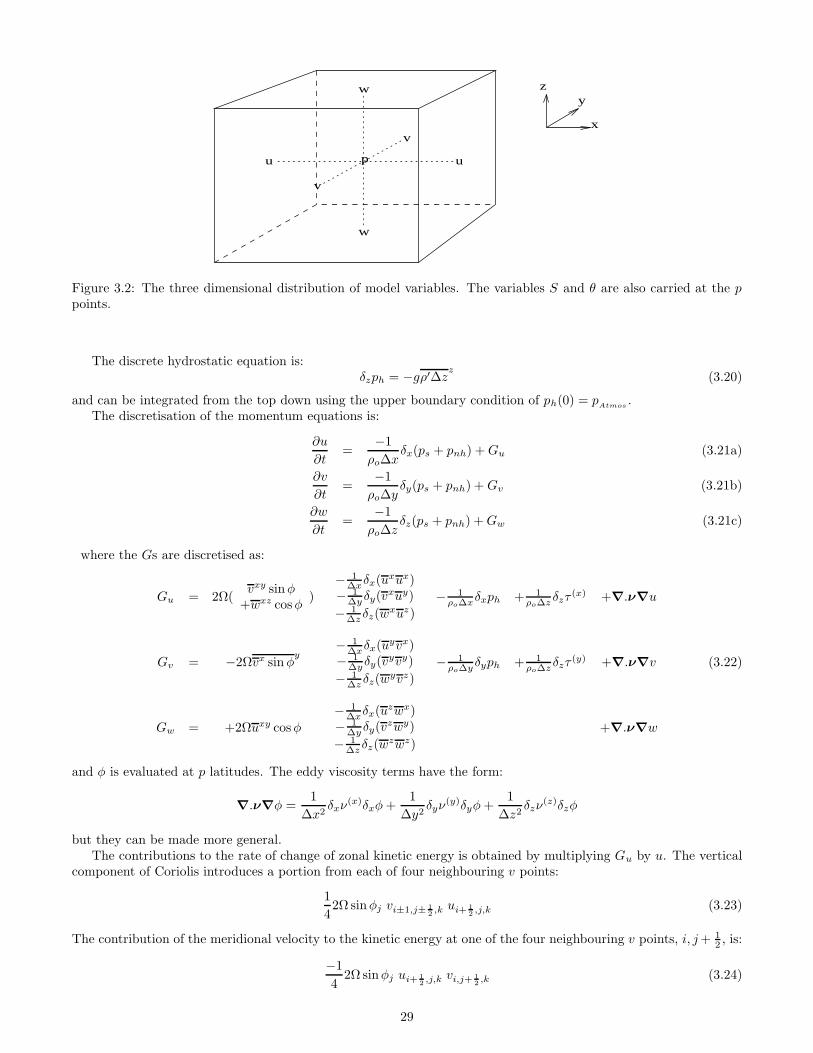
u

v

v

w

w

up

x

yz

Figure 3.2: The three dimensional distribution of model variables. The variables S and θ are also carried at the ppoints.

The discrete hydrostatic equation is:δzph = −gρ′∆zz (3.20)

and can be integrated from the top down using the upper boundary condition of ph(0) = pAtmos

.The discretisation of the momentum equations is:

∂u

∂t=

−1

ρo∆xδx(ps + pnh) +Gu (3.21a)

∂v

∂t=

−1

ρo∆yδy(ps + pnh) +Gv (3.21b)

∂w

∂t=

−1

ρo∆zδz(ps + pnh) +Gw (3.21c)

where the Gs are discretised as:

Gu = 2Ω(vxy sinφ

+wxz cosφ)

− 1∆xδx(u

xux)− 1

∆yδy(vxuy)

− 1∆z δz(w

xuz)

− 1ρo∆xδxph + 1

ρo∆z δzτ(x) +∇.ν∇u

Gv = −2Ωvx sinφy

− 1∆xδx(u

yvx)− 1

∆yδy(vyvy)

− 1∆z δz(w

yvz)

− 1ρo∆yδyph + 1

ρo∆z δzτ(y) +∇.ν∇v

Gw = +2Ωuxy cosφ

− 1∆xδx(u

zwx)− 1

∆yδy(vzwy)

− 1∆z δz(w

zwz)

+∇.ν∇w

(3.22)

and φ is evaluated at p latitudes. The eddy viscosity terms have the form:

∇.ν∇φ =1

∆x2δxν

(x)δxφ+1

∆y2δyν

(y)δyφ+1

∆z2δzν

(z)δzφ

but they can be made more general.The contributions to the rate of change of zonal kinetic energy is obtained by multiplying Gu by u. The vertical

component of Coriolis introduces a portion from each of four neighbouring v points:

1

42Ω sinφj vi±1,j± 1

2,k ui+ 1

2,j,k (3.23)

The contribution of the meridional velocity to the kinetic energy at one of the four neighbouring v points, i, j+ 12 , is:

−1

42Ω sinφj ui+ 1

2,j,k vi,j+ 1

2,k (3.24)

29

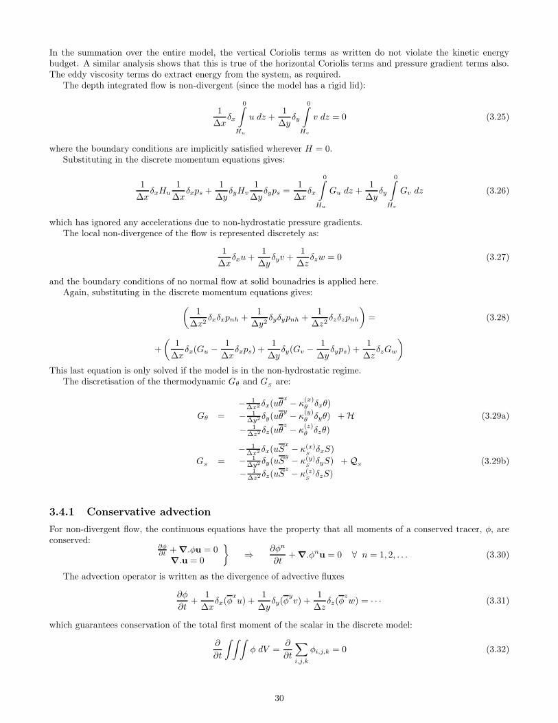
In the summation over the entire model, the vertical Coriolis terms as written do not violate the kinetic energybudget. A similar analysis shows that this is true of the horizontal Coriolis terms and pressure gradient terms also.The eddy viscosity terms do extract energy from the system, as required.

The depth integrated flow is non-divergent (since the model has a rigid lid):

1

∆xδx

0∫

Hu

u dz +1

∆yδy

0∫

Hv

v dz = 0 (3.25)

where the boundary conditions are implicitly satisfied wherever H = 0.Substituting in the discrete momentum equations gives:

1

∆xδxHu

1

∆xδxps +

1

∆yδyHv

1

∆yδyps =

1

∆xδx

0∫

Hu

Gu dz +1

∆yδy

0∫

Hv

Gv dz (3.26)

which has ignored any accelerations due to non-hydrostatic pressure gradients.The local non-divergence of the flow is represented discretely as:

1

∆xδxu+

1

∆yδyv +

1

∆zδzw = 0 (3.27)

and the boundary conditions of no normal flow at solid bounadries is applied here.Again, substituting in the discrete momentum equations gives:

(

1

∆x2δxδxpnh +

1

∆y2δyδypnh +

1

∆z2δzδzpnh

)

= (3.28)

+

(

1

∆xδx(Gu − 1

∆xδxps) +

1

∆yδy(Gv −

1

∆yδyps) +

1

∆zδzGw

)

This last equation is only solved if the model is in the non-hydrostatic regime.The discretisation of the thermodynamic Gθ and G

Sare:

Gθ =

− 1∆x2 δx(uθ

x − κ(x)θ δxθ)

− 1∆y2 δy(uθ

y − κ(y)θ δyθ)

− 1∆z2 δz(uθ

z − κ(z)θ δzθ)

+ H (3.29a)

GS

=

− 1∆x2 δx(uS

x − κ(x)SδxS)

− 1∆y2 δy(uS

y − κ(y)SδyS)

− 1∆z2 δz(uS

z − κ(z)SδzS)

+ QS

(3.29b)

3.4.1 Conservative advection

For non-divergent flow, the continuous equations have the property that all moments of a conserved tracer, φ, areconserved:

∂φ∂t + ∇.φu = 0

∇.u = 0

⇒ ∂φn

∂t+ ∇.φnu = 0 ∀ n = 1, 2, . . . (3.30)

The advection operator is written as the divergence of advective fluxes

∂φ

∂t+

1

∆xδx(φ

xu) +

1

∆yδy(φ

yv) +

1

∆zδz(φ

zw) = · · · (3.31)

which guarantees conservation of the total first moment of the scalar in the discrete model:

∂

∂t

∫ ∫ ∫

φ dV =∂

∂t

∑

i,j,k

φi,j,k = 0 (3.32)

30

The x component of the flux form can be re-arranged using rule 3.12e:

δx(φxu) = φδxu+ uδxφ

x(3.33)

and the same can be done for the y and z terms. Substituting into the advection term gives:

∂φ

∂t+

1

∆xuδxφ

x+

1

∆yvδyφ

y+

1

∆zwδzφ

z+ φ

(

δxu

∆x+δyv

∆y+δzw

∆z

)

= · · · (3.34)

where the last term vanishes if the flow is non-divergent according to this definition.Multiplying by φ gives:

∂ φ2

2

∂t+

1

∆xφuδxφ

x+

1

∆yφvδyφ

y+

1

∆zφwδzφ

z= · · · (3.35)

Considering only the x direction, the advective term can be written:

φuδxφx

= uφxδxφ

x

− 1

4δx (uδxφδxφ) (3.36)

where use has been made of 3.12g. The last term can be re-written using a special case of 3.12f:

− 1

4δx (uδxφδxφ) = δx

(

u(φxφx − φ2

x))

(3.37)

and then introducing the unconventional notation via 3.14:

φuδxφx

= δx

(

u1

2o φo2x

)

− φ2

2δxu (3.38)

Repeating the procedure for the other two contributions gives a flux form for the second moment of the scalar:

∂ φ2

2

∂t+

1

∆xδx(u o φo2x) +

1

∆yδy(v o φo2y) +

1

∆zδz(w o φo2z) −

φ2

2

(

δxu

∆x+δyv

∆y+δzw

∆z

)

= · · · (3.39)

where once again, if the flow is non-divergent the last term vanishes.The same advection scheme is applied to the momentum equations, though here, the advecting flow must be

interpolated appropriately. To advect u in the conservative manner just described, the advecting u∗, v∗ and w∗ mustbe interpolated from u, v and w in such a way as to be non-divergent.

u∗ = ux v∗ = vx w∗ = wx (3.40)

Expanding the divergence of the advecting flow and making use of the commutativity between interpolation anddifference operators yields:

δxu∗

∆x+δyv

∗

∆y+δzw

∗

∆z=δxu

x

∆x+δyv

x

∆y+δzw

x

∆z=δxu

∆x+δyv

∆y+δzw

∆z

x

= 0 (3.41)

Therefore, the total of zonal, meridional and vertical velocity contributions to the kinetic energy are conserved bythe advection operator.

Higher moments of momentum and scalars are not conserved. Higher order differencing and forms of advectioncould perhaps be used to achieve this. Here, the efficiency and simplicity of the numerical model was deemed moreimportant than conservation of higher moments.

3.5 The time-stepping scheme (Adams-Bashforth II)

Consider the horizontal momentum equations in an abbreviated form:

∂

∂tu = P (p) + G(u,x, t) (3.42)

where P contains the horizontal pressure gradient and is therefore a function only of the pressure field. All otherterms that appear in the horizontal momentum equations are grouped into G which will then be a function of thevelocities, space and time.

31

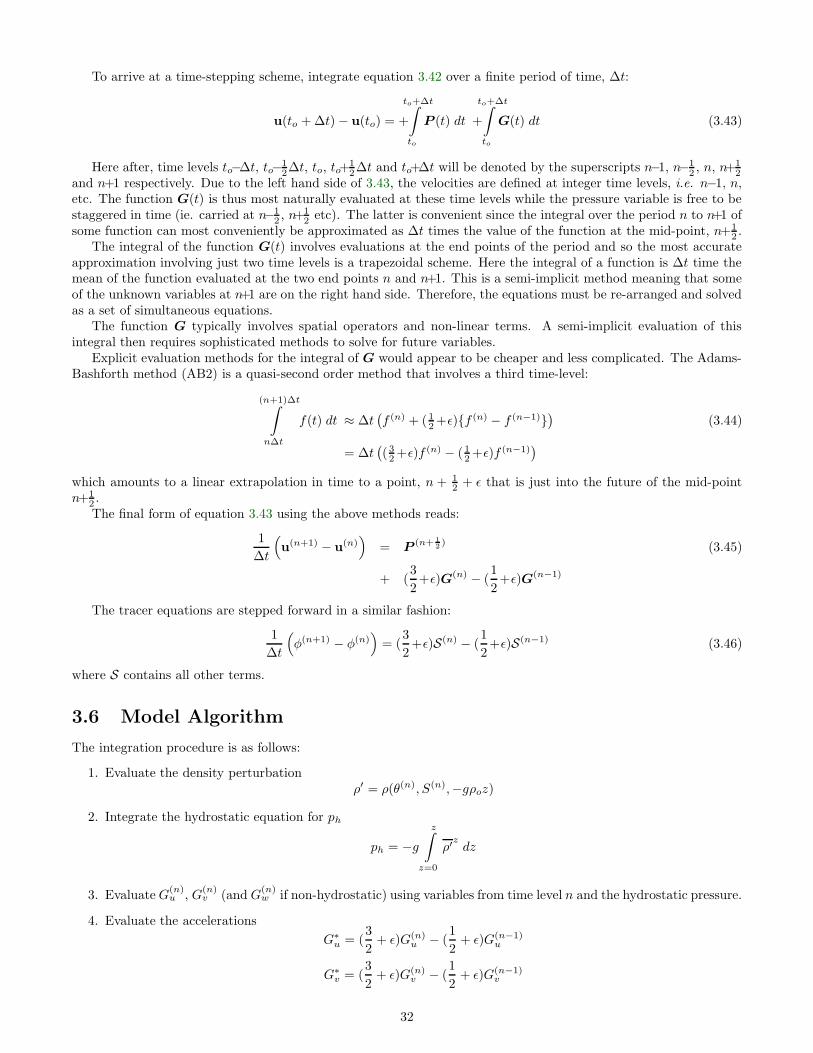
To arrive at a time-stepping scheme, integrate equation 3.42 over a finite period of time, ∆t:

u(to + ∆t) − u(to) = +

to+∆t∫

to

P (t) dt +

to+∆t∫

to

G(t) dt (3.43)

Here after, time levels to−∆t, to−12∆t, to, to+

12∆t and to+∆t will be denoted by the superscripts n−1, n−1

2 , n, n+12

and n+1 respectively. Due to the left hand side of 3.43, the velocities are defined at integer time levels, i.e. n−1, n,etc. The function G(t) is thus most naturally evaluated at these time levels while the pressure variable is free to bestaggered in time (ie. carried at n−1

2 , n+12 etc). The latter is convenient since the integral over the period n to n+1 of

some function can most conveniently be approximated as ∆t times the value of the function at the mid-point, n+12 .

The integral of the function G(t) involves evaluations at the end points of the period and so the most accurateapproximation involving just two time levels is a trapezoidal scheme. Here the integral of a function is ∆t time themean of the function evaluated at the two end points n and n+1. This is a semi-implicit method meaning that someof the unknown variables at n+1 are on the right hand side. Therefore, the equations must be re-arranged and solvedas a set of simultaneous equations.

The function G typically involves spatial operators and non-linear terms. A semi-implicit evaluation of thisintegral then requires sophisticated methods to solve for future variables.

Explicit evaluation methods for the integral of G would appear to be cheaper and less complicated. The Adams-Bashforth method (AB2) is a quasi-second order method that involves a third time-level:

(n+1)∆t∫

n∆t

f(t) dt ≈ ∆t(

f (n) + ( 12 +ε)f (n) − f (n−1)

)

= ∆t(

( 32 +ε)f (n) − ( 1

2 +ε)f (n−1))

(3.44)

which amounts to a linear extrapolation in time to a point, n + 12 + ε that is just into the future of the mid-point

n+12 .The final form of equation 3.43 using the above methods reads:

1

∆t

(

u(n+1) − u(n))

= P (n+ 12) (3.45)

+ (3

2+ε)G(n) − (

1

2+ε)G(n−1)

The tracer equations are stepped forward in a similar fashion:

1

∆t

(

φ(n+1) − φ(n))

= (3

2+ε)S(n) − (

1

2+ε)S(n−1) (3.46)

where S contains all other terms.

3.6 Model Algorithm

The integration procedure is as follows:

1. Evaluate the density perturbationρ′ = ρ(θ(n), S(n),−gρoz)

2. Integrate the hydrostatic equation for ph

ph = −gz

∫

z=0

ρ′zdz

3. EvaluateG(n)u , G

(n)v (and G

(n)w if non-hydrostatic) using variables from time level n and the hydrostatic pressure.

4. Evaluate the accelerations

G∗u = (

3

2+ ε)G(n)

u − (1

2+ ε)G(n−1)

u

G∗v = (

3

2+ ε)G(n)

v − (1

2+ ε)G(n−1)

v

32

If non-hydrostatic

G∗w = (

3

2+ ε)G(n)

w − (1

2+ ε)G(n−1)

w

5. Solve the elliptic problem

δxHuδxps + δyHvδyps = δx

0∫

Hu

(u(n)

∆t+G∗

u) dz + δy

0∫

Hv

(v(n)

∆t+G∗

v) dz

for the surface pressure, ps. This guarantees that the depth integrated flow will be non-divergent at the nexttime level.

6. If non-hydrostatic, solve the elliptic problem

[δxδx + δyδy + δzδz]pnh = δx(u(n)

∆t+G∗

u − δxps) + δy(v(n)

∆t+G∗

v − δyps) + δz(w(n)

∆t+G∗

w)

for the non-hydrostatic pressure, otherwise let pnh = 0.

7. Update horizontal velocities:

u(n+1) = u(n) + ∆t

(

G∗u −

1

ρoδx(ps + pnh)

)

v(n+1) = v(n) + ∆t

(

G∗v −

1

ρoδy(ps + pnh)

)

8. Integrate the continuity equation for w

w(n+1) = −z

∫

H

(δxu(n=1) + δyv

(n+1)) dz

9. Evaluate the Gs for θ and S using the latest velocities.

10. Update the thermodynamic variables

θ(n+1) = θ(n) + ∆t

(

(3

2+ ε)G

(n)θ − (

1

2+ ε)G

(n−1)θ + H(\)

)

S(n+1) = S(n) + ∆t

(

(3

2+ ε)G

(n)S − (

1

2+ ε)G

(n−1)S + Q(\)

S

)

11. Update indices: n→ n+ 1 and repeat procedure for the next time-step.

3.7 3-D Elliptic Inversion

The diagnostic equation for pressure is a three dimensional Poisson equation and once discretised, takes the form ofa sparse matrix equation: A p = f

Despite the sparse nature of A, the inverse A−1 is a dense matrix which reflects the elliptic nature of the problem.

Direct evaluation of the inverse A−1, even for a moderately sized grid, is impractical due to the storage of A−1 and

to the number of operations required when multiplying A−1f . Instead, the sparse matrix equation is solved using apre-conditioned conjugate gradient algorithm.

The algorithm uses an approximate inverse, A−1

(called the pre-conditioner) to find a correction to the currentestimate of the solution. Repeated iteration converges in a finite number of steps to within a finite tolerance, ε. Thepre-conditioner is used in each iteration. The convergence rate is improved as the pre-conditioner approaches thetrue inverse, but obviously, the sparser the pre-conditioner is, the fewer the number of computations required periteration.

A pre-conditioner was designed that is efficient in both storage and number of operations and is a good approxi-mation to A−1. This is accomplished by taking advantage of the geometry of the ocean. The ocean is typically onlya few kilometres deep but as much as several thousand kilometres wide. This leads to a dominance in the Laplacian

operator, ∇23, by the vertical contribution, ∂2

∂z2 . In the sparse matrix corresponding to the 3D Laplacian, just threeof the diagonals dominate the seven non-zero diagonals. Retaining just these three diagonals, LU decomposition canbe applied rather than storing the inverse of the tri-diagonal. This also reduces the number of computations.

33

ro = f −A po

bo = A−1po

↓αi =

[ri,A

−1r

i]

[bi,A b

i]

pi+1

= pi+ αibi ri+1 = ri − αiA bi

βi =[r

i+1,A

−1r

i+1]

[ri,A

−1r

i]

bi+1 = A−1ri+1 + βibi

↓ ↑ n[ri+1, ri+1] < ε2

↓ yStop

Figure 3.3: Flow diagram for the pre-conditioned conjugate gradient algorithm

Figure 3.4: Schematic of the ocean domain, decomposed into columns (dashed lines) to which individual processorsare dedicated. The shaded regions represents land and the irregular boundaries of the ocean. The stencil representsthe local connectivity of the Laplacian operator. The solid dots within the stencil represent the dominant coefficientsin the Laplacian and the only connection in the pre-conditioner.

3.8 Computational Aspects of Model: Data parallel architectures

We concentrate our code development on the CM-5, a distributed memory architecture. The code is written inCM-Fortran, a vendor release of Data Parallel Fortran or Fortran 90.

The distributed memory architecture of the CM-5 means that inter-processor communication is an importantfactor in programming the machine efficiently. The decomposition of arrays into the machines memory can be chosento reduce the number of cross-processor transfer of information.

The most costly task in the model is the elliptic inversion (whether 2-D or 3-D). The decomposition and thealgorithm were both designed to optimize this stage of the model; a significant part of the CPU time is spent in theconjugate gradient algorithm described above. The two principal operators involved here are the Laplacian operatorand the pre-conditioner. The Laplacian operator entails nearest neighbour connections between grid points in allthree spatial directions (white and black points in figure 3.4). The pre-conditioner connects grid-points only in avertical line (black points only in figure 3.4). Accordingly, the domain is decomposed into vertical columns, thatreach from the top to the bottom of the ocean. This means that vertically aligned points in the model are residenton the same processor thus reducing the communication to zero for the pre-conditioning stage; half of the algorithm.

34

3.9 Applications of the model

The model has been developed for use at all scales of oceanographic interest. For example, the non-hydrostaticversion of the model is applicable to the study of convective overturning. The hydrostatic version of the model canbe used to study larger scales right up to the global scale.

By way of illustration of the versatility of the model, two experiments at extreme ends of the spectrum scales arebriefly described. The first is a high resolution simulation (∆x = 500m) of open ocean convection and the latter isa comparatively low resolution study (∆x ∼ 100km) of the North Pacific Ocean.

3.9.1 Baroclinic instability of a chimney (convection site)

The non-hydrostatic model is initially at rest with a weak stratification (N 2 = 5 × 10−8 s−2) in a box 64 km ×64 km × 2 km. The horizontal and vertical resolutions are 500 m and 100 m respectively. Cooling is continuouslyapplied at the surface in a disc of radius 8 km (with a random spatial component). The fluid convectively overturns,fluxing heat upward from the interior to balance the forcing. A mean radial gradient in temperature is establishedwhich becomes baroclinically unstable. At some point it becomes more efficient for the fluid to flux heat laterallythan vertically so that baroclinic instability begins to dominate.

Figure 3.5 shows the density anomaly at z=-250m after 10 days. The sharp gradients indicate the front, formedat the edge of the convective zone or chimney, that is undergoing baroclinic instability. This figure is reproducedcourtesy of Helen Jones of Legg et al., 1995 [LJVPO].

The model behaves very well in this high resolution limit. There is little grid scale noise. The parallel design ofthe conjugate gradient algorithm used to solve the 3D elliptic problem is very effective.

10 20 30 40 50 60

10

20

30

40

50

60

Domain Distance (km)

Dom

ain

Dis

tanc

e (k

m)

Figure 3.5: Density anomaly at z=-250m at day 10 in a convection experiment. Reproduced courtesy of Helen Jones(see text).

35

3.9.2 Climatological spin-up of the North Pacific Ocean

An extended regional calculation is made to obtain a state of the North Pacific Ocean suitable for initializingsubsequent integrations. Here, a realistic stratification is desired and so the model is forced with observational data.

The GCM is integrated in hydrostatic mode for the Pacific Ocean (31S to 61N, 122E 293E). It has realisticcoast-lines and bottom topography. Bottom and side walls are insulating. A no-slip (free-slip) condition is used atside walls (bottom). The horizontal grid resolution is 1. There are 20 levels, with a minimum layer thickness of 25m at the top to a maximum thickness of 500 m at the bottom.

At the surface, the model is relaxed to climatological values of temperature and salinity [Lev82] with a relaxationtime scale of 25 days. At the southern boundary, the relaxation is made over a 5o zone with a time scale of 5 daysat the boundary, decreasing linearly to 100 days at 26S.

The model was initialized from climatological annual mean temperature and salinity distributions [Lev82] anda resting flow field. It was integrated for 17 years with annual mean temperature, salinity and surface wind stressforcing. From year 18 onwards, monthly temperatures, seasonal salinities and monthly winds [TOL89] were used.The forcing fields were updated daily by linearly interpolating from the monthly or seasonal data. Surface heat andfreshwater fluxes [Obe88] were introduced in the surface layer starting in year 29. The model time step is 1 hour.The mixing and diffusion coefficients are presented in table 3.1.

Figures 3.6, 3.7 and 3.8 show the state of the model at the end of year 43. The solution exhibits the main featuresof the observed circulation including the Kuroshio and Oyashio Currents.

This integration used an implementation of the Cd scheme that will be described in chapter 5. Without this inno-vation, the above integration would not have been possible since the unmodified C grid is susceptible to developmentof grid scale noise.

To demonstrate the nature of the problem inherent in an unmodified C grid model, the integration was carriedon for just one more month after year 43 using the unmodified C grid version of the GCM. Figures 3.9 and 3.10 showthe vertical velocity at the end of the extra month. Grid length waves emanate from the boundaries. The wavesare predominant at high latitudes where the Rossby radius of deformation is not resolved. With time, the noisepropagates through out the model and eventually masks the large scale signal. Note that at the upper level, theocean is relatively well stratified and that the noise has not reached the interior whilst in the deep, weakly stratifiedocean, the noise has penetrated to the Equator.

Horizontal Mixing νh 5 × 103

Vertical Mixing νz 10−3

Horizontal Diffusion κh 5 × 103

Vertical Diffusion κz 3 × 10−5

Table 3.1: GCM mixing and diffusion coefficients for the North Pacific spin-up. Units are m2 s−1.

36

140 160 180 200 220 240 260 280−30

−20

−10

0

10

20

30

40

50

60

Longitude

Latit

ude

−0.7 −0.6−0.6

−0.5

−0.5

−0.4

−0.3

−0.2

−0.2

−0.1

−0.1

−0.1

−0.1

0

0

0

0

00

0.1

0.1

0.1

0.1

0.10.1

0.2

0.2

0.2

0.3

0.4

0.5

0.6

Figure 3.6: Pressure (in m) at z=-12.5 m at end of year 43.

−30 −20 −10 0 10 20 30 40 50 60

−5000

−4500

−4000

−3500

−3000

−2500

−2000

−1500

−1000

−500

0

Latitude

Dept

h

1.5

2

2

3

4

5

7

7

99

11

1417

20 23

Figure 3.7: Temperature (in oC) at λ=171.5E at end of year 43.

−30 −20 −10 0 10 20 30 40 50 60

−5000

−4500

−4000

−3500

−3000

−2500

−2000

−1500

−1000

−500

0

Latitude

Dept

h

34.5

34.6

34.6

35.135.3

Figure 3.8: Salinity (in psu) at λ=171.5E at end of year 43.

37

140 160 180 200 220 240 260 280−30

−20

−10

0

10

20

30

40

50

60

Longitude

Latit

ude

Figure 3.9: Vertical velocity at the base of the top layer in the model after one month of integration with the Cd

scheme switched off. Note the presence of grid length waves. Contour interval is 0.01 mm s−1.

140 160 180 200 220 240 260 280−30

−20

−10

0

10

20

30

40

50

60

Longitude

Latit

ude

Figure 3.10: Vertical velocity at z=-3200m in the model after one month. Only the zero contour is shown. The gridlength noise is more prevalent at depth because of the weaker stratification.

38

3.9.3 Conventional treatments of grid scale noise

There have been many attempts in the past to control noise level in ocean models, most frequently in ‘C’ gridformulations that are particularly sensitive to noise at low resolutions.

Several methods that were implemented during the development of the global ocean model are mentioned belowbut this should by no means be considered a definitive comparison.

Deformation dependent diffusion is a method described by Smagorinsky [Sma63], Deardorff [Dea71] and Smithand Bleck [SBB90] in which the lateral diffusion parameter is a function of the local deformation of the flow. Inprinciple, the deformation field reflects the amplitude of grid-scale noise and acts to smooth the model fields wherethe noise is manifest. The scheme is physically appealing in that it leaves the physics unaffected except where noiseis generated. In practice, a large diffusion coefficient is needed to effectively reduce the noise level and the explicit(in time) evaluation procedure easily violates the numerical stability criteria. An implicit implementation can beemployed here but was not investigated.

Biharmonic diffusion This is a commonly used method that is more scale selective than Laplacian diffusion.The method is appealing in that the large scale dynamics is left untouched. In practice again, large coefficients arerequired but with the limited coefficients allowed for stability (in the explicit model) the method was found to be atleast as effective as divergence damping.

Divergence damping This method is based on some understanding of the source of the noise [Xu94]. A non-physical term is added to the horizontal momentum equations; Dtu+ ... = ∇hλD where D = ∇h.uh is the horizontaldivergence. On taking the curl of the momentum equations, it should be apparent that the vorticity dynamics isleft unaffected whilst the divergence equation (the poor representation of which is the source of the noise) has anadditional diffusion term. This scheme seemed appealing because of this ability to selectively damp noise in thedivergence field and in practice seemed to be quite effective in reducing the noise level. A large coefficient, λ, isrequired but not so large as to cause numerical instability. The only cause for concern was the unfortunate effect atthe equator where the dynamics are as much a function of the horizontal divergence field as they are of the vorticity.The sharp upwelling patterns at the equator become very smoothed. In principle, λ could be made a function oflatitude to overcome this problem but this was not investigated.

More drastic methods can also be used, such as periodic filtering of the model fields. This would at least be honestin that it deals directly with the noise rather than via the introduction of some “artificial” terms. In practice, noneof the above methods work perfectly. They control the problem by reducing the noise level. They all manage thisby damping. Wherever there is a source of noise, damping is not good enough. Balancing a source against dampingresults in a finite amplitude signal.

Instead, the source of the problem should be re-considered. The principle issue here is the gridding. For the ‘C’grid, the ability to support grid-scale noise is a direct consequence of the spatial averaging required to evaluate theCoriolis terms. Before deriving a method by which this problem is avoided, it is necessary to revisit the theory thatdescribes the grid-noise phenomenon in the model. The next chapter discusses shallow water theory, the propagationof inertia-gravity waves and the finite difference representation of these waves before describing a method that avoidsthe grid-noise problem.

39

Chapter 4

Numerical Representation ofInertia-Gravity Waves

Here, we discuss the representation of inertia-gravity waves in finite difference models. The representation of Rossbywaves will be considered in the following chapter.

The first sections of the chapter describe Shallow Water theory. It is in this dynamical formulation that the natureof inertia-gravity waves is most accessible. Further more, numerical issues (in particular, the choice of gridding) aretraditionally examined in this context.

Having developed an understanding of how the continuous model behaves, an analysis of discrete models onvarious grids shows how the numerical waves behave as a function of scale. Of particular interest here, is the effectof averaging used in evaluating the Coriolis term on the C grid. The averaging allows grid-scale noise to persist. Thenoise is manifest in the divergence field and is excited in ocean models by the narrow layers of wind-driven upwellingat boundaries.

The analysis of Arakawa and Lamb, 1977 [AL77], suggests that two particular formulations (the B and C gridsusing their notation) are most suitable for modeling rotating fluids. To study gridding choices two numerical modelswere built and integrated in a variety of configurations. The results of the integrations are consistent with thepredictions of the numerical analysis.

Whenever models are operating at sub-optimum resolutions, grid-scale noise results and is normally removed byfiltering or damping. Instead of dealing with the noise in this crude manner, a philosophy of dealing with the causeof the problem is adopted. Section 4.6 describes a new numerical scheme for treating the Coriolis term on a C gridthat accurately represents the inertia-gravity waves and thus avoids the spurious grid-noise problems inherent in the‘C’ grid.

The inertia-gravity waves are found to be well behaved at all resolutions using the new scheme. Despite this,there is a new kind of grid-scale noise that appears in the presence of the planetary vorticity gradient, β. The reasonfor this is that the scheme fails to accurately represent short Rossby waves. This problem will be discussed and dealtwith in the next chapter.

4.1 Shallow Water Theory

The dynamics of a homogeneous layer of fluid were briefly analysed in chapter 2. Here two such layers of differentdensity will be considered (see figure 4.1). The two layer system has two intrinsic modes; the barotropic and baroclinicmodes. The modes can be separated in the linear system. Although the behavior of linear internal inertia-gravitywaves (section 2.4.1) was shown to be quite analogous to the linear external gravity wave discussed previously, it ismore appropriate to derive the equations governing the baroclinic mode.

The inviscid, linear, Boussinesq momentum equations on a β-plane for a homogeneous layer are:

∂u

∂t− fo(1 +

βy

fo)v +

1

ρo

∂p

∂x= 0 (4.1a)

∂v

∂t+ fo(1 +

βy

fo)u+

1

ρo

∂p

∂y= 0 (4.1b)

gρ+∂p

∂z= 0 (4.1c)

∇h.uh +∂w

∂z= 0 (4.1d)

40

(x,y)

z

ρ2

ρ1

p=g

H(x,y)

H(x,y)

2

1h

ρη

Figure 4.1: The shallow water model comprises of two homogeneous layers of fluid (ρ1, ρ2) between rigid-lids, with afree interface of perturbation elevation h. The pressure exerted by the rigid-lid is equivalent to a surface elevation η.

The rigid-lid at the surface exerts a pressure on the fluid of gρ1η, where η is the inferred displacement of thesurface. Integrating the hydrostatic relation between some arbitrary depth z and the surface z = 0 yields:

p(x, y, z) =

po + gρ1(η − z) ∀h−H1 < z < ηpo + gρ1(η − h+H1) + gρ2(h−H1 − z) ∀H2 < z < h−H1

(4.2)

and consequently, horizontal gradients of pressure are independent of depth within the layers:

∇p1 = gρ1ρo

∇η

∇p2 = gρ1ρo

∇(η − h) + gρ2ρo

∇h(4.3)

The continuity equation can be applied to each layer to give the rate of change of elevation of the interface:

− ∂h

∂t+ ∇ · (H1 − h)u1 = 0 (4.4)

+∂h

∂t+ ∇ · (h+H2)u2 = 0 (4.5)

These equations can be weighted by 1H1

and 1H2

respectively and added to give:

(

1

H1+

1

H2

)

∂h

∂t+ ∇ · (u2 − u1) = O(

hu2

H2) + · · · (4.6)

where the non-linear contributions will be small if the interface perturbation is assumed to be small compared to H1

and H2 (h H1, H2).Defining:

u = u2 − u1

g∗ =gρ1

ρo

g′ =g

ρo(ρ2 − ρ1)

H∗ =H1H2

H1 +H2

41

the shallow water equations for the baroclinic mode u can be written:

∂

∂tu + fo(1 +

βy

fo)k ∧ u + g′∇h = 0 (4.7a)

∂h

∂t+H∗

∇ · u = 0 (4.7b)

These equations are prognostic in all three dependent variables which makes the shallow water equations themost simple to integrate numerically (due to the absence of any kind of elliptic inverse problem). For the purpose ofanalysis, the linearity the equations is also very convenient.

If H1 < H2 then H∗ must fall in the range 12H1 ≤ H∗ < H1. Typically, the bottom layer will be much deeper

than the top layer (H1 << H2) and so H∗ ∼ H1, where a summer time upper-layer depth might be 30 m.A representative density contrast is ρ2−ρ1

ρo∼ 10−3 so that g′ ∼ 10−2. The gravity wave speed, which will be

derived shortly, is√g′H∗ ∼ 0.54ms−1, much slower than the external gravity wave speed

√gH ∼ 10 − 100ms−1.

Assuming that u and v scale in a similar fashion, then the equations can be non-dimensionalised and written interms of external parameters. The horizontal velocities are non-dimensionalised by a typical velocity scale U . Letthe horizontal length scale of the motion be L for a typical interface displacement of ho and the time-scale be f−1

o

then the non-dimensional equations may be written:

∂

∂tu + (1 + βy)k ∧ u +

g′hofoLU

∇h = 0 (4.8a)

f−1o hoL

H∗U

∂h

∂t+ ∇ · u = 0 (4.8b)

where all the variables are now non-dimensional. Here, β is the non-dimensional planetary vorticity gradient,β → βL

fo.

The non-dimensional quantity in the momentum equations can be expressed:

g′hofoLU

=g′H∗

U2

h

H∗

U

foL= RiδRo (4.9)

where Ri = g′H∗

U2 =c2gU2 is the Richardson number and Ro = U

foLis the Rossby number. δ = h

H∗ is a small parametermeasuring the magnitude of perturbation elevation against the vertical scale height H∗.

Similarly, the non-dimensional number appearing in the continuity equation can be expressed:

f−1o hoL

H∗U=hoH

foL

U= δR−1

o (4.10)

Since, the time-scales of interest are longer than f−1o , then for the non-dimensional velocity to be order one, the

pressure gradient term should be order one also. The internal parameter δ can therefore be chosen:

δRiRo = 1 (4.11)

The non-dimensional shallow water equations are then:

∂

∂tu + (1 + βy)k ∧ u + ∇h = 0 (4.12a)

S−1 ∂h

∂t+ ∇ · u = 0 (4.12b)

where the non-dimensional parameter S = RiR2o = g′H∗

f2oL

2 =L2

ρ

L2 is the Burger number, which is the square of the

ratio between the Rossby deformation radius and the length scale. This ratio will prove to be very relevant when ananalysis of the numerical models is made. The crucial quantity will be the Burger number of the grid-scale, bettertermed the wave resolution.

The kinetic and potential energy take the forms KE = 12u · u, PE = 1

2S−1h2. Total energy,

∫∫

KE + PE dA, isconserved in the absence of external forces.

The shallow water equations derived here are analogous to the barotropic equations describing the externalgravity mode. The system exhibits all of the properties pertinent to an individual baroclinic mode of the hydrostaticprimitive equations. This model was derived for this property so that it can be used as a elementary setting toanalyse the numerical models.

42

4.2 Inertia-Gravity Waves

The Coriolis terms in isolation act to make the flow move in inertial circles. The pressure gradient terms allow apressure anomaly to propagate as a gravity wave. In conjunction, both motions are described by a pair of inertia-gravity wave modes as follows. The divergence, vorticity and continuity equations are:

∂

∂tD − ζ + ∇

2h = 0 (4.13a)

∂

∂tζ +D = 0 (4.13b)

S−1 ∂

∂th+D = 0 (4.13c)

The inertia-gravity waves are best described in terms of the divergence field. Differentiating the divergence equationand eliminating the vorticity and pressure terms yields a wave equation of the form:

∂2

∂t2D +D − S∇

2D = 0 (4.14)

Substituting a plain wave solution of the form eı(kx+ly−ωt) into the wave equation yields the dispersion relation forthe inertia-gravity waves:

ω2 = 1 + S(k2 + l2) (4.15)

The frequency, ω, of a gravity wave is thus a monotonically increasing function in |κ| =√k2 + l2, with a minimum

frequency of ω = 1 corresponding to S = 0 or κ = 0. For long waves, S|κ|2 << 1, the frequency is approximatelyω ≈ 1 and so the dominant frequency is set by the Coriolis acceleration. For short waves, S|κ|2 >> 1, the frequencybecomes proportional to the wave number, ω ≈

√S|κ|. In this limit, the pressure gradient terms are the predominant

ones controlling the wave propagation.The group velocity, ∂ω

∂kis:

cg =S

√

1 + S|κ|2

(

kl

)

and always points in the direction of the wave vector, κ. For the long waves the group speed is proportional to thewave number cg ≈ Sκ while for short waves the group speed asymptotes to cg =

√S 1

|κ|(k, l). Never does the group

speed approach zero for non-zero k or l.This, then, is how linear inertia gravity waves propagate in the continuum. Although a discrete representation

cannot be expected to reproduce this behavior perfectly, it is useful to examine the dispersion relation and groupspeed on the grid to assess the closeness of the numerical representation of the dynamics to that of the real oceanand so qualitatively gauge the numerical scheme. A celebrated account of this analysis was given by Arakawa andLamb [AL77] which will be summarised later.

4.3 Damped wave motion

The inertia-gravity wave motions just described allow the fluid to adjust to a geostrophic state. In an inviscidmodel, the gravity waves travel and reflect off boundaries, unimpaired by diffusion. Such a model would neverreach a steady state. Dissipation of some form must be represented. Accordingly, an arbitrary operator, F , willbe introduced to represent the dissipation. Damping of the continuity equation can also be introduced, H , whichreflects the dissipation in the buoyancy equation of the primitive equations.

∂

∂tu + k ∧ u + ∇h = F (u) (4.16a)

∂

∂th+ S∇ · u = H(h) (4.16b)

As before, the three dependent variables can easily be exchanged for two dependent variables by expressing theequations in terms of divergence, vorticity and elevation, and then eliminating the vorticity:

(∂

∂t− F )2D +D + (

∂

∂t− F )∇2h = 0 (4.17a)

(∂

∂t− H)h+ SD = 0 (4.17b)

43

h,u,v

u,v

u,vu,v

u,v

h hu

v

u

v

u

u

vv

u,v

u,v

u,v u,vh h

h h

h h

A

ED

CB

Figure 4.2: The variables of a model can be arranged in only five grids that maintain second order accuracy. GridsA-D share the same grid-spacing. Grid E is equivalent to the B grid rotated through 45o and scaled by

√2.

In the special case where H = F , the gravity wave motion is easily found by eliminating h:

(∂

∂t− F )2D +D + S∇

2D = 0 (4.18)

which gives the dispersion relation:ω = ıF ±

(

1 + S(k2 + l2))

(4.19)

The real, oscillatory part of ω is just the plain inertia-gravity wave contribution from the inviscid model;±

(

1 + S(k2 + l2))

. The imaginary, decaying part is simply the damping rate of the operator for that particularwave number. The inertia-gravity waves are damped, but the phase and group speeds of the oscillatory solutionremain unchanged.

4.4 Finite-differenced Inertia-gravity waves

Using centered finite differencing and the simplest single-level time stepping scheme, the shallow water equations canbe discretised on five distinct grids (see figure 4.2). Arakawa and Lamb [AL77], for the purpose of analysis, assumedthat the time-stepping scheme was perfect and retained the continuous time derivative. It is in fact quite simpleto consider discrete time-stepping but as long as the scheme is centered (and thus second order accurate), no newconsequences arise.

Scheme A:

δtu− vt + δxhx

= 0 (4.20a)

δtv + ut + δyhy

= 0 (4.20b)

S−1δth+ (δxux + δyv

y) = 0 (4.20c)

Scheme B:

δtu− vt + δxhy

= 0 (4.21a)

δtv + ut + δyhx

= 0 (4.21b)

S−1δth+ (δxuy + δyv

x) = 0 (4.21c)

44

Scheme C:

δtu− vxyt + δxh = 0 (4.22a)

δtv + uxyt + δyh = 0 (4.22b)

S−1δth+ (δxu+ δyv) = 0 (4.22c)

Scheme D:

δtu− vxyt + δxhxy

= 0 (4.23a)

δtv + uxyt + δyhxy

= 0 (4.23b)

S−1δth+ (δxuxy + δyv

xy) = 0 (4.23c)

The E grid is omitted since it is equivalent to the B grid rotated through 45o and scaled by√

2.The divergence equations for each model are as follows:A grid:

D ≡ δxux + δyv

y δttD +Dtt − S(δxxD

xx+ δyyD

yy) = 0 (4.24)

B grid:

D ≡ δxuy + δyv

x δttD +Dtt − S(δxxD

yy+ δyyD

xx) = 0 (4.25)

C grid:

D ≡ δxu+ δyv δttD +Dxxyytt − S(δxxD + δyyD) = 0 (4.26)

D grid:

D ≡ δxu+ δyv δttD +Dtt − S(δxxD + δyyD)

xxyy

= 0 (4.27)

Substitution of a plane wave solution (exp ı(kx+ ly − ωt)) into the divergence equations yields:

A: ω2 = 1 + S(s2kc2k + s2l c

2l ) (4.28a)

B: ω2 = 1 + S(s2kc2l + s2l c

2k) (4.28b)

C: ω2 = c2kc2l + S(s2k + s2l ) (4.28c)

D: ω2 = c2kc2l + Sc2kc

2l (s

2k + s2l ) (4.28d)

where the abbreviations, sk = 2∆x sin k∆x

2 , sl = 2∆y sin l∆y2 , ck = cos k∆x

2 and cl = cos l∆y2 have been used forbrevity. In the limit of infinitely high spatial resolution, ck → 1 and sk → k, etc. Thus all the finite differencedispersion relations approach the continuous limit though they may still contain extra turning points.

The common term Ss2k = 4S∆x2 sin2 k∆x/2 is the discrete analogue of Sk2. The quantity 4S/∆x2 is the wave

resolution parameter, which appears in all the dispersion relations. It is the square of the ratio between twice thedimensional Rossby deformation radius and the dimensional grid-spacing. If 4S/∆x2 = 1, the grid spacing is smallenough to resolve a single wavelength equal to the deformation radius. High resolution corresponds to 4S/∆x2 1and low resolution to 4S/∆x2 1.

Figure 4.4 shows the non-dimensional frequency as a function of wave resolution, m = k∆x/π, n = l∆x/π forhigh resolution models on the four different grids. For comparison, the analytic dispersion relation for the continuoussystem is plotted in figure 4.3 for the same mode numbers.

The gradient of the surfaces is the group velocity and should always be directed away from the origin. At highresolution, the discrete dispersion relations might be expected to approach the analytic result as the resolutionincreases. This is always found but the discrete cases always contain extra minima at the highest wave numbers.

The A grid has three erroneous minima occurring at the two grid-scale wave length; m = 1, n = 1 and m = n = 1.Between these points and the turning points (m = 1/2 and n = 1/2) the group velocity has the wrong sign. Thephase speed is underestimated because the frequency of motion is much lower than it should be.

The B grid has one extra minima for the checker board mode (grid-scale mode number in each direction, m =n = 1). The group velocity has the wrong sign for short waves that satisfy m+ n > 1. Again, the phase speed andfrequency are severely underestimated but this time only in one quadrant.

The C grid underestimates the frequency of the highest modes. In the analytic case, the frequency reachedapproximately 2.5 cycles whilst the peak C grid frequency is about 2 cycles. The group speed is always of the rightsign with the highest errors at high wave numbers.

45

0 0.2 0.4 0.6 0.8 1

00.2

0.40.6

0.811

2

3

4

5

6

mn

w

Figure 4.3: Non-dimensional frequency of the continuous spectrum is plotted against non-dimensional wave numberm,n. The discrete wave numbers allowed in the model are represented by the grid-lines. The wave numberscorrespond to the next figure where 4S

∆x2 = 2.

0 0.5 10

0.5

1

1.2

1.4

1.6

1.8

2

mn

w

A grid

0 0.5 10

0.5

1

1.2

1.4

1.6

1.8

2

mn

w

B grid

0 0.5 10

0.5

1

1.2

1.4

1.6

1.8

2

mn

w

C grid

0 0.5 10

0.5

10

0.5

1

1.5

2

mn

w

D grid

Figure 4.4: Non-dimensional frequency of the discrete waves is plotted against wave-resolution m,n. The Rossbyradius is resolved, 4S

∆x2 = 2. The discrete wave numbers allowed in the model are represented by the grid-lines.

46

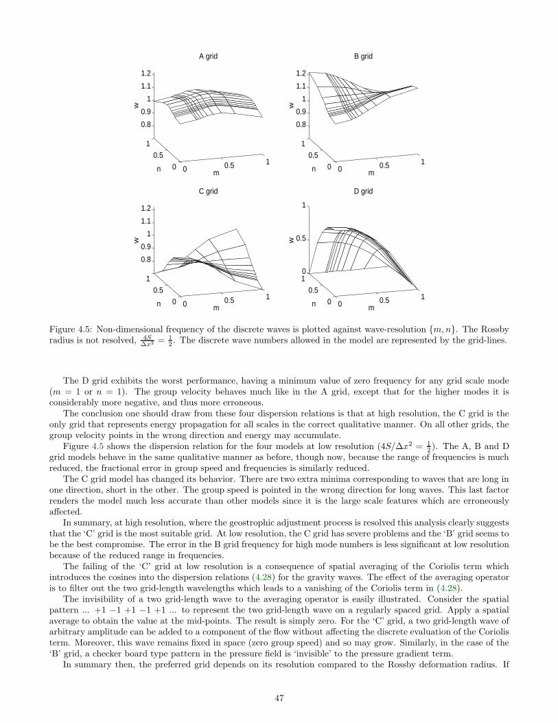
0 0.5 10

0.5

1

0.8

0.9

1

1.1

1.2

mn

w

A grid

0 0.5 10

0.5

1

0.8

0.9

1

1.1

1.2

mn

w

B grid

0 0.5 10

0.5

1

0.8

0.9

1

1.1

1.2

mn

w

C grid

0 0.5 10

0.5

10

0.5

1

mn

w

D grid

Figure 4.5: Non-dimensional frequency of the discrete waves is plotted against wave-resolution m,n. The Rossbyradius is not resolved, 4S

∆x2 = 12 . The discrete wave numbers allowed in the model are represented by the grid-lines.

The D grid exhibits the worst performance, having a minimum value of zero frequency for any grid scale mode(m = 1 or n = 1). The group velocity behaves much like in the A grid, except that for the higher modes it isconsiderably more negative, and thus more erroneous.

The conclusion one should draw from these four dispersion relations is that at high resolution, the C grid is theonly grid that represents energy propagation for all scales in the correct qualitative manner. On all other grids, thegroup velocity points in the wrong direction and energy may accumulate.

Figure 4.5 shows the dispersion relation for the four models at low resolution (4S/∆x2 = 12 ). The A, B and D

grid models behave in the same qualitative manner as before, though now, because the range of frequencies is muchreduced, the fractional error in group speed and frequencies is similarly reduced.

The C grid model has changed its behavior. There are two extra minima corresponding to waves that are long inone direction, short in the other. The group speed is pointed in the wrong direction for long waves. This last factorrenders the model much less accurate than other models since it is the large scale features which are erroneouslyaffected.

In summary, at high resolution, where the geostrophic adjustment process is resolved this analysis clearly suggeststhat the ‘C’ grid is the most suitable grid. At low resolution, the C grid has severe problems and the ‘B’ grid seems tobe the best compromise. The error in the B grid frequency for high mode numbers is less significant at low resolutionbecause of the reduced range in frequencies.

The failing of the ‘C’ grid at low resolution is a consequence of spatial averaging of the Coriolis term whichintroduces the cosines into the dispersion relations (4.28) for the gravity waves. The effect of the averaging operatoris to filter out the two grid-length wavelengths which leads to a vanishing of the Coriolis term in (4.28).

The invisibility of a two grid-length wave to the averaging operator is easily illustrated. Consider the spatialpattern ... +1 −1 +1 −1 +1 ... to represent the two grid-length wave on a regularly spaced grid. Apply a spatialaverage to obtain the value at the mid-points. The result is simply zero. For the ‘C’ grid, a two grid-length wave ofarbitrary amplitude can be added to a component of the flow without affecting the discrete evaluation of the Coriolisterm. Moreover, this wave remains fixed in space (zero group speed) and so may grow. Similarly, in the case of the‘B’ grid, a checker board type pattern in the pressure field is ‘invisible’ to the pressure gradient term.

In summary then, the preferred grid depends on its resolution compared to the Rossby deformation radius. If

47

this length scale is not resolved then the shortest resolved scales of motion are aware of the Coriolis effect and so the’B’ grid is the better choice. If this length scale is resolved, then the shortest motions will be gravity waves and thedominant process controlling their evolution will be the pressure gradient term and so the ‘C’ grid will be the betterchoice.

This criterion works well if the deformation radius is relatively fixed, both in time and space. However, in baro-clinic models of the atmosphere and oceans, the deformation radius is a function of latitude, the local stratificationand the vertical wave number of the particular baroclinic mode, L(m)

D= N/f(φ)m−1, where m is the dimensional

vertical wave number, f(φ) is the local Coriolis parameter and N is the local Brunt-Vasala frequency. Thus, with afixed grid, there is the possibility of both resolving and not resolving the local deformation radius in separate partsof a model, or for different vertical modes.

In the case of the GCM described in chapter 3, the model is used to study the global scale circulation. Thisdemands a coarse resolution because of the limitations of the computer. Hence a ‘B’ grid might be argued for. Here,however, the model is also used to study convection which demands the the formulation on a C grid.

4.5 Numerical Shallow Water models

Having developed a linear tool to study grid-scale noise in the GCM, it remains to test the ideas in practice. Sinceonly two models, the ‘B’ and ‘C’ grids, are expected to be reliably accurate (depending on wave resolution), thesewere the ones developed.

The shallow water models described earlier were second order accurate in time. This meant that the evaluationof the Coriolis term was made in a semi-implicit manner. Implicit Coriolis terms on the A and B grids involvessimple algebraic manipulation of the discretised equations. On the C and D grids, because of the spatial averaging,implementing implicit Coriolis terms involves finding the inverse of a matrix describing the spatial dependencies.

In order to compare models to examine the effects of gridding choice, these models should use the same algorithmswherever possible in order to isolate the cause of any differences. The C grid restricts the modeller to an explicitevaluation of the Coriolis terms (for a reasonably efficient code). In all of the following models, the quasi-secondorder Adams-Bashforth scheme is applied to evaluate the Coriolis terms.

The B and C grid models will now be described. The same grid resolutions are used in both whenever the modelsare compared. The grid resolution is defined by the number of pressure points in each direction. Thus, the pressurefield is carried at the same physical locations in each model. Both models carry the normal velocity on the physicalboundaries. The B grid also carries the tangential velocity on the boundary and an extra boundary condition is thusneeded here. The simplest choice is that of no-slip.

The models are forced with an analytically described wind stress. Dissipation is parameterised by a linear frictionlike term with time-scale λ−1. Had a higher order diffusion term been chosen, the grid-scale noise would be moreefficiently removed and the discrepancies between the two grids less obvious.

4.5.1 B grid shallow water model

The grid of the B grid model is defined by cells centered about the pressure point, h. For M ×N pressure points,there are therefore (M + 1) × (N + 1) points that carry the velocities u and v, although 2(M +N) of these lie onthe boundary.

The time-stepping cycle is comprised of two prognostic steps; one stepping forward the continuity equation andthe other stepping forward the momentum equations.

The continuity equation is time differenced as described before; single time level with a centered in time andspace evaluation of the divergence field:

hn+ 12 = hn−

12 + ∆tS

(

δxuny

+ δyvnx)

(4.29)

No flux through solid boundaries is a necessary condition to evaluate the right hand side. The initial state is one ofno motion.

The next stage in the model time-step is to step forward the momentum equations as follows:

un+1 = un + ∆t(

+(1 + εβy)v(n+ 1

2) − δxhn+ 1

2

y

+ τx − λun)

(4.30a)

vn+1 = vn + ∆t(

−(1 + εβy)u(n+ 1

2) − δyhn+ 1

2

x

+ τy − λvn)

(4.30b)

where the parenthesized superscript (n+ 12 ) denotes the Adams-Bashforth extrapolation: u(n+ 1

2) = ( 3

2 + εAB)un −( 12 + εAB)un−1. No flow normal to solid boundaries is imposed in the continuity equation.

48

Low Highresolution resolution

Burger number S 1.0× 10−4 6.25× 10−2

Planetary vorticity gradient β 0.0 0.0Friction λ 3 × 10−2 3 × 10−2

Time step ∆t 0.2 0.2Adams-Bashforth parameter εAB 0.1 0.1Grid spacing ∆x = ∆y 1/10 1/10

Wave resolution 2√S/∆x 1/5 5

Table 4.1: External parameters used in the comparison of the B and C grid shallow water models. High resolutionmeans that the Rossby deformation radius is resolved whilst Low resolution means that it is not.

4.5.2 C grid shallow water model

As in the B grid model, the C grid is defined by cells centered about the pressure point, h. For M × N pressurepoints, there are therefore (M + 1) ×N points that carry the zonal velocity, u, and M × (N + 1) points that carrythe meridional velocity, v.

The time-stepping cycle is as for the B grid. The continuity equation is time differenced with a single time levelwith a centered in time and space evaluation of the divergence field:

hn+ 12 = hn−

12 + ∆tS (δxu

n + δyvn) (4.31)

The vanishing of the normal flux through solid boundaries is applied quite naturally.The momentum equations are stepped forward as follows:

un+1 = un + ∆t(

+(1 + εβy)v(n+ 12)xy

− δxhn+ 1

2 + τx − λun)

(4.32a)

vn+1 = vn + ∆t(

−(1 + εβy)u(n+ 12)xy

− δyhn+ 1

2 + τy − λvn)

(4.32b)

where the parenthesized superscript (n) again denotes the Adams-Bashforth extrapolation: u(n) = ( 32 + εAB)un −

( 12 + εAB)un−1.

4.5.3 Shallow water model results

The B and C grid models described above were configured to mimic a double gyre on an f-plane. The modelextents were x : 0 ≤ x ≤ 1 and y : −1 ≤ y ≤ 1. The applied wind stress was circular and non-divergent,

τ = k ∧ ∇(sinπx sinπy) where the appropriate discrete operator was used to evaluate the curl.The external parameters of the models are listed in table 4.1. The Burger number is defined using the physical

zonal extent of the basin, S = L2D/L2. The wave resolution is thus 2

√S/∆x and was 5 for the high resolution run

and 1/5 for the low. The symmetric forcing and absence of β effect (εβ = 0) means that the solutions should besymmetric.

Low resolution: Figures 4.6 and 4.7 show the low resolution B and C grid models at t = 100. The wave resolutionis 2

√S/∆x = 1/5. At this resolution the B grid reproduces the analytical solution very well. The pressure field

and divergence patterns in the B grid both reflect the structure of the forcing. The C grid however is clearly beinginfluenced by boundary effects. The large values of upwelling and downwelling at the boundaries alternate as onemoves from the boundary. In the corners, the alternating zonal and meridional patterns interfere to produce achecker-board pattern. All three of the short wave combinations (meridional, zonal, checker-board) correspond tothe minimum frequencies in the dispersion relation of the C grid. The erroneous pressure field in the C grid is alsodriving fast flows which bear no relation to the more reasonable circulation of the B grid.

These integrations mimic the previous low resolution integrations of the GCM. The grid-scale noise is similar incharacter. The conclusion here is that a GCM developed on a B grid would perform better at low resolution.

High resolution: The high resolution integrations tell a different tale. Figures 4.8 and 4.9 show the high resolutionB and C grid models at t = 100. The resolution is now 2

√S/∆x = 5. The pressure field and circulation both appear

49

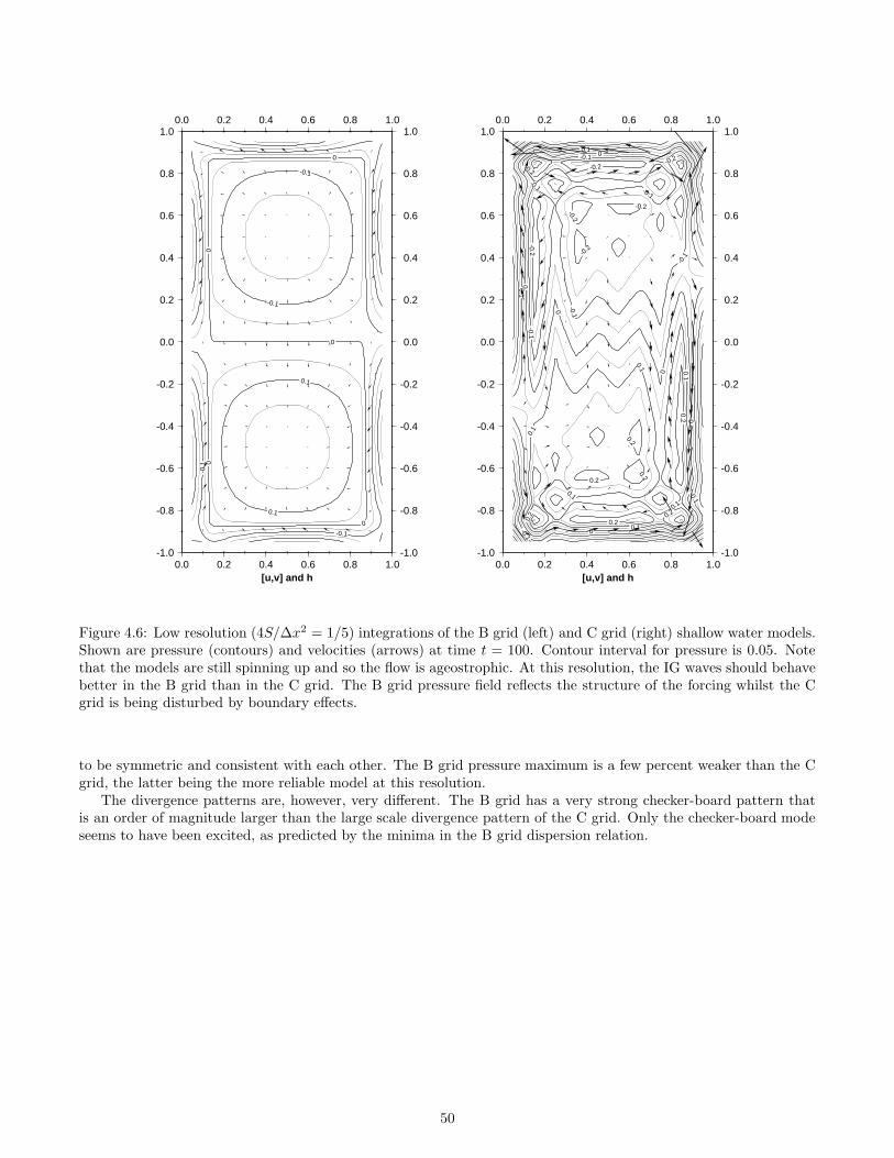
-0.1

-0.1

-0.1

-0.1

0

0

0

0

0

0.1

0.1

-1.0

-0.8

-0.6

-0.4

-0.2

0.0

0.2

0.4

0.6

0.8

1.0

-1.0

-0.8

-0.6

-0.4

-0.2

0.0

0.2

0.4

0.6

0.8

1.0

0.0 0.2 0.4 0.6 0.8 1.0

0.0 0.2 0.4 0.6 0.8 1.0

[u,v] and h

-0.2 -0.2-0.2

-0.2

-0.2

-0.2

-0.2

-0.1

-0.1

-0.1

-0.1

-0.1

-0.1

-0.1

-0.1

0

0

0

0

0

0

0.1

0.1

0.1

0.10.

1

0.1

0.1

0.1

0.2

0.2

0.2

0.2

0.2

0.20.2

-1.0

-0.8

-0.6

-0.4

-0.2

0.0

0.2

0.4

0.6

0.8

1.0

-1.0

-0.8

-0.6

-0.4

-0.2

0.0

0.2

0.4

0.6

0.8

1.0

0.0 0.2 0.4 0.6 0.8 1.0

0.0 0.2 0.4 0.6 0.8 1.0

[u,v] and h

Figure 4.6: Low resolution (4S/∆x2 = 1/5) integrations of the B grid (left) and C grid (right) shallow water models.Shown are pressure (contours) and velocities (arrows) at time t = 100. Contour interval for pressure is 0.05. Notethat the models are still spinning up and so the flow is ageostrophic. At this resolution, the IG waves should behavebetter in the B grid than in the C grid. The B grid pressure field reflects the structure of the forcing whilst the Cgrid is being disturbed by boundary effects.

to be symmetric and consistent with each other. The B grid pressure maximum is a few percent weaker than the Cgrid, the latter being the more reliable model at this resolution.

The divergence patterns are, however, very different. The B grid has a very strong checker-board pattern thatis an order of magnitude larger than the large scale divergence pattern of the C grid. Only the checker-board modeseems to have been excited, as predicted by the minima in the B grid dispersion relation.

50

-10

-10

0

0

0

0

0

10

10

-1.0

-0.8

-0.6

-0.4

-0.2

0.0

0.2

0.4

0.6

0.8

1.0

-1.0

-0.8

-0.6

-0.4

-0.2

0.0

0.2

0.4

0.6

0.8

1.0

0.0 0.2 0.4 0.6 0.8 1.0

0.0 0.2 0.4 0.6 0.8 1.0

δxu + δyv

-20

-20 -20 -2

0

-20-20-20

-10

-10

-10

-10

-10

-10

-10

-10

0

00

0

0

0

10

10

10

10

10

10

10

10

20

2020 20

20

20

20

-1.0

-0.8

-0.6

-0.4

-0.2

0.0

0.2

0.4

0.6

0.8

1.0

-1.0

-0.8

-0.6

-0.4

-0.2

0.0

0.2

0.4

0.6

0.8

1.0

0.0 0.2 0.4 0.6 0.8 1.0

0.0 0.2 0.4 0.6 0.8 1.0

δxu + δyv

Figure 4.7: Low resolution (4S/∆x2 = 1/5) integrations of the B grid (left) and C grid (right) shallow water models.Shown is the horizontal divergence at time t = 100. Contour interval is 5. The flow is ageostrophic at this stage inthe integration so the divergence is still large. The C grid clearly has more signal at the grid scale than does the Bgrid.

51

-20

-15

-15

-10

-10

-5-5

-5

0

0

0

0

5

5

5

10

10

15

15

20

-1.0

-0.8

-0.6

-0.4

-0.2

0.0

0.2

0.4

0.6

0.8

1.0

-1.0

-0.8

-0.6

-0.4

-0.2

0.0

0.2

0.4

0.6

0.8

1.0

0.0 0.2 0.4 0.6 0.8 1.0

0.0 0.2 0.4 0.6 0.8 1.0

[u,v] and h

-25

-20

-20

-15

-15

-10

-10

-10

-5

-5

-5

5

5

5

10

10

10

15

15

20

20

25

-1.0

-0.8

-0.6

-0.4

-0.2

0.0

0.2

0.4

0.6

0.8

1.0

-1.0

-0.8

-0.6

-0.4

-0.2

0.0

0.2

0.4

0.6

0.8

1.0

0.0 0.2 0.4 0.6 0.8 1.0

0.0 0.2 0.4 0.6 0.8 1.0

[u,v] and h

Figure 4.8: High resolution (4S/∆x2 = 5) integrations of the B grid (left) and C grid (right) shallow water models.Shown are pressure (contours) and velocities (arrows) at time t = 100. Contour interval for pressure is 1. The modelsare approaching the steady state so the flow is nearly geostrophic. But for slightly different maximum values, themodels would appear to be in good agreement. The divergence patterns (next figure) show that this is not the case.

52

-20

-20

-20-20

-20 -20

-10-10

-10

-10

-10

-10

-10

-10

-10

-10

-10

-10

-10

-10

-10

00

0

0

0

0

0

0

0

0

0

0

1010

10

10

10

10

10

10

10

10

1010

10

10 10

20

20

2020

20

20

-1.0

-0.8

-0.6

-0.4

-0.2

0.0

0.2

0.4

0.6

0.8

1.0

-1.0

-0.8

-0.6

-0.4

-0.2

0.0

0.2

0.4

0.6

0.8

1.0

0.0 0.2 0.4 0.6 0.8 1.0

0.0 0.2 0.4 0.6 0.8 1.0

δxu + δyv

-1

0

0

0

1

-1.0

-0.8

-0.6

-0.4

-0.2

0.0

0.2

0.4

0.6

0.8

1.0

-1.0

-0.8

-0.6

-0.4

-0.2

0.0

0.2

0.4

0.6

0.8

1.0

0.0 0.2 0.4 0.6 0.8 1.0

0.0 0.2 0.4 0.6 0.8 1.0

δxu + δyv

Figure 4.9: High resolution (4S/∆x2 = 5) integrations of the B grid (left) and C grid (right) shallow water models.Shown is the horizontal divergence at time t = 100. Contour interval is 0.5 for the B grid and 5 for the C grid.The flow is nearly geostrophic at this stage in the integration so the divergence is small. The C grid clearly has nogrid-scale noise. The B grid has a grid-scale signal, one order of magnitude larger than the smooth signal of the Cgrid.

53

4.6 The Explicit Oscillator Algorithm

In both B and C grid formulations, problems arise through the need to interpolate variables to their ‘unnatural’positions. A 2∆x wave is invisible when viewed through the averaging operator x implying that the physicsrepresented by that term cannot act at that particular wave number. Thus on the B grid, a 2∆x wave cannot beaware of the presence of pressure gradient forces normal to the wave vector, though this is relatively unimportant atlarge scales. Similarly on the C grid, a 2∆x wave cannot feel Coriolis effects. In short, averaging is an undesirablefeature in both these finite difference models.

In the case of the C grid, examination of equation (4.26) suggests that if one could ensure that spatial averaging

did not occur in the oscillation term, f 2Dtt, then the dispersion relation would approach the analytic limit to the

maximum extent possible using second order finite differencing. This can be achieved as follows. Consider the forcedoscillator form of the horizontal momentum equations:

u = uov = vo

t = 0 (4.33a)

∂∂tu− fv = X∂∂tv + fu = Y

t ≥ 0 (4.33b)

Here, X = X(x, y, z, t) and Y = Y (x, y, z, t) contain all other terms in the horizontal momentum equations. Thisis completely equivalent to the system:

u = uov = vo


t = 0 (4.34a)

∂2

∂t2 u− f ∂∂tv = ∂

∂tX∂2

∂t2 v + f ∂∂tu = ∂

∂tY

t ≥ 0 (4.34b)

By substituting for the acceleration f ∂∂t (u, v) in equations 4.34b from 4.33b, the complete system can be written

as a set of four initial conditions and two oscillator equations coupled through the forcing functions X and Y :

u = uov = vo


t = 0 (4.35a)

∂2

∂t2u+ f2u = ∂∂tX + fY

∂2

∂t2 v + f2v = ∂∂tY − fX

t ≥ 0 (4.35b)

A discrete form for 4.35b might take the form:

δttu+ f2utt = δtX + fYtxy

(4.36a)

δttv + f2vtt = δtY − fXtxy

(4.36b)

and so propagation of the inviscid inertia-gravity waves would be determined by:

1

f2δttD +D

tt − L2ρ(δxxD + δyyD) = 0 (4.37)

which leads to the dispersion relation:

4

f2∆t2sin2 ω∆t

2= cos2

ω∆t

2+

4L2ρ

∆x2

(

sin2 k∆x

2+ sin2 l∆x

2

)

(4.38)

Unlike their counter-parts on a C grid, equation 4.37 does not have any averaging operators at all. This is becausethe pressure terms within the interpolated operators of 4.36 cancel and so do not feature in 4.37. For this reason, itcan be expected that the dispersion relation will not suffer from the deficiencies of the C grid formulation.

54

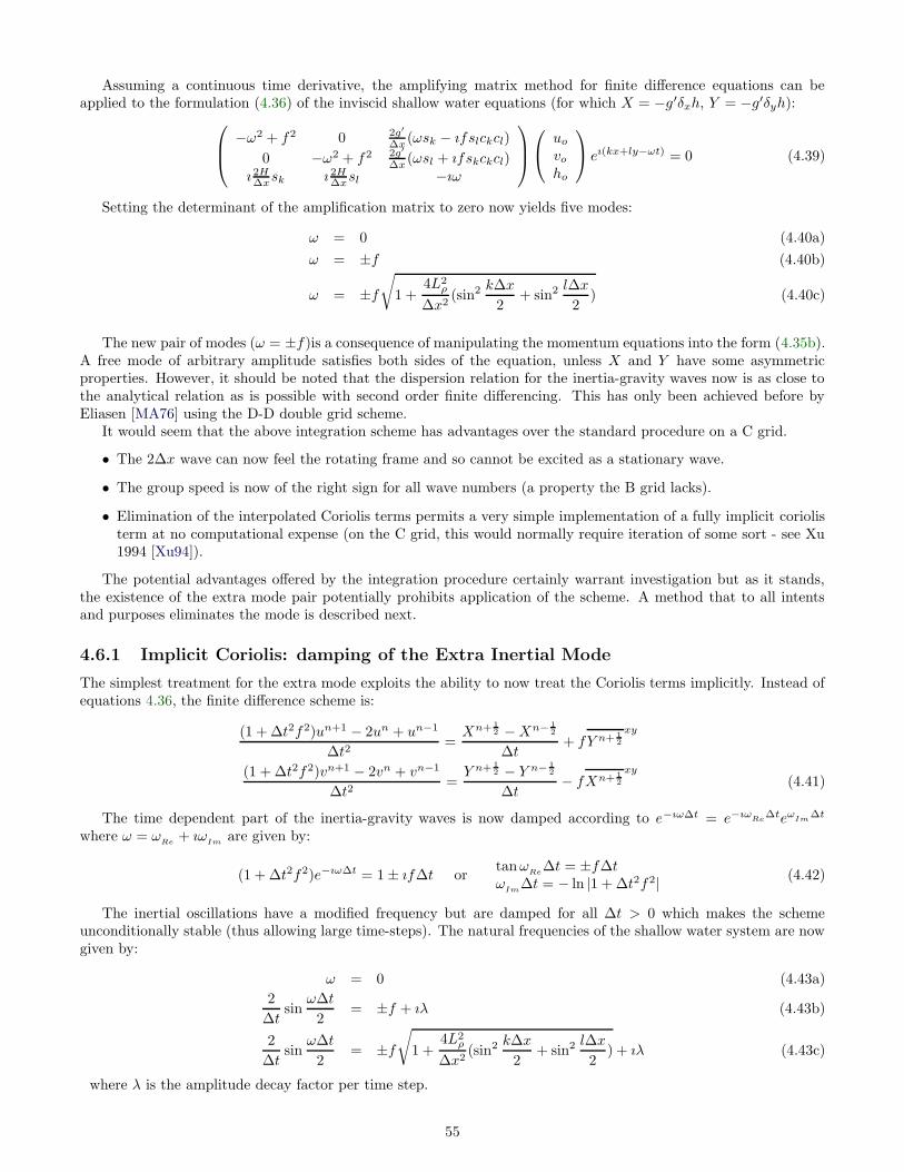
Assuming a continuous time derivative, the amplifying matrix method for finite difference equations can beapplied to the formulation (4.36) of the inviscid shallow water equations (for which X = −g′δxh, Y = −g′δyh):

−ω2 + f2 0 2g′

∆x(ωsk − ıfslckcl)

0 −ω2 + f2 2g′

∆x(ωsl + ıfskckcl)ı 2H∆xsk ı 2H∆xsl −ıω

uovoho

eı(kx+ly−ωt) = 0 (4.39)

Setting the determinant of the amplification matrix to zero now yields five modes:

ω = 0 (4.40a)

ω = ±f (4.40b)

ω = ±f√

1 +4L2

ρ

∆x2(sin2 k∆x

2+ sin2 l∆x

2) (4.40c)

The new pair of modes (ω = ±f)is a consequence of manipulating the momentum equations into the form (4.35b).A free mode of arbitrary amplitude satisfies both sides of the equation, unless X and Y have some asymmetricproperties. However, it should be noted that the dispersion relation for the inertia-gravity waves now is as close tothe analytical relation as is possible with second order finite differencing. This has only been achieved before byEliasen [MA76] using the D-D double grid scheme.

It would seem that the above integration scheme has advantages over the standard procedure on a C grid.

• The 2∆x wave can now feel the rotating frame and so cannot be excited as a stationary wave.

• The group speed is now of the right sign for all wave numbers (a property the B grid lacks).

• Elimination of the interpolated Coriolis terms permits a very simple implementation of a fully implicit coriolisterm at no computational expense (on the C grid, this would normally require iteration of some sort - see Xu1994 [Xu94]).

The potential advantages offered by the integration procedure certainly warrant investigation but as it stands,the existence of the extra mode pair potentially prohibits application of the scheme. A method that to all intentsand purposes eliminates the mode is described next.

4.6.1 Implicit Coriolis: damping of the Extra Inertial Mode

The simplest treatment for the extra mode exploits the ability to now treat the Coriolis terms implicitly. Instead ofequations 4.36, the finite difference scheme is:

(1 + ∆t2f2)un+1 − 2un + un−1

∆t2=Xn+ 1

2 −Xn− 12

∆t+ fY n+ 1

2

xy

(1 + ∆t2f2)vn+1 − 2vn + vn−1

∆t2=Y n+ 1

2 − Y n−12

∆t− fXn+ 1

2

xy

(4.41)

The time dependent part of the inertia-gravity waves is now damped according to e−ıω∆t = e−ıωRe∆teωIm

∆t

where ω = ωRe

+ ıωIm

are given by:

(1 + ∆t2f2)e−ıω∆t = 1 ± ıf∆t ortanω

Re∆t = ±f∆t

ωIm

∆t = − ln |1 + ∆t2f2| (4.42)

The inertial oscillations have a modified frequency but are damped for all ∆t > 0 which makes the schemeunconditionally stable (thus allowing large time-steps). The natural frequencies of the shallow water system are nowgiven by:

ω = 0 (4.43a)

2

∆tsin

ω∆t

2= ±f + ıλ (4.43b)

2

∆tsin

ω∆t

2= ±f

√

1 +4L2

ρ

∆x2(sin2 k∆x

2+ sin2 l∆x

2) + ıλ (4.43c)

where λ is the amplitude decay factor per time step.

55

4.6.2 Comparison to the standard models

Figures 4.10 and 4.11 show the circulation, pressure and divergence fields at t = 100, for a C grid model that evaluatesthe momentum equations in the manner described above. The external parameters were identical to the analogousB and pure C grid integrations. A consequence of implementing the method just described is that the damping ratesdue to the implicit evaluation of Coriolis and the Adams-Bashforth extrapolation of the previous two models aredifferent. This should not affect the final steady state but may change the convergence rate and phase of transients.

We conclude from these integrations that this ‘oscillator’ scheme does effectively correct the source of grid-scalenoise resulting from inertia-gravity waves on the C grid at low resolution. At high resolution, the solution is unaffected(ie. is as accurate as the pure C grid) though the phase of the solution will obviously only match that of an implicitC grid model.

The scheme is, however, flawed for a physical reason which has not yet been discussed. Figure 4.12 shows thedouble gyre circulation on a β-plane obtained using the above scheme. A two-grid length wave, parallel to themeridional boundaries is clearly evident and seems to emanate from the western boundary.

A brief explanation of its origins is as follows. In the long term, the flow should become geostrophically balanced.Normally, on a ‘C’ grid, geostrophic balance takes the form:

fuxy

= −δyh fvyx

= δxh (4.44)

Now, the steady state form of equation 4.36 defines the geostrophic flow as:

fu = −δyhxy

fv = δxhxy

(4.45)

The averaging operator now appears in the slowly evolving geostrophic component of the flow. Grid-scale noise in thepressure field is filtered by the interpolation and not felt by the geostrophic circulation. Indeed, the solution (figure4.12) shows a perfectly smooth Sverdrupian circulation, despite the high noise level in the pressure and divergencefields.

In summary, just as the Coriolis term on a C grid is invisible to grid scale noise in the flow field, the pressuregradient term in the geostrophic balance is invisible to grid scale noise in the pressure field. This implies that theshortest Rossby waves are poorly represented.

56

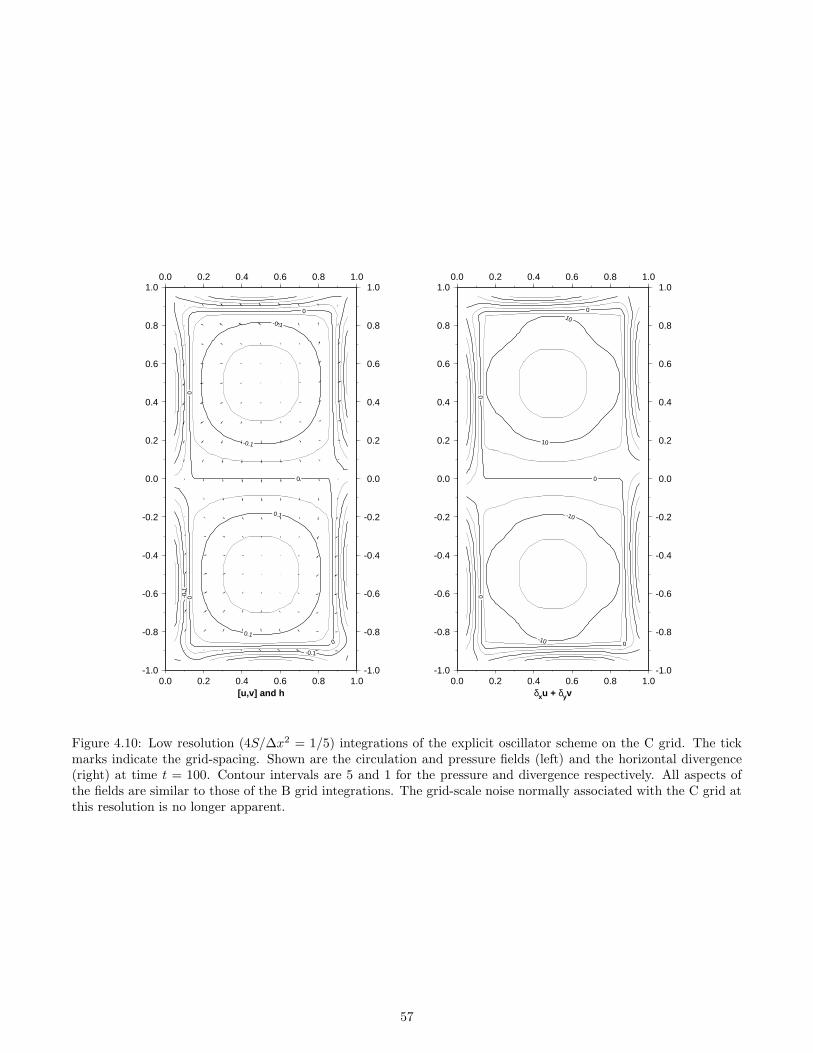
-0.1

-0.1

-0.1

-0.1

0

0

0

0

0

0.1

0.1

-1.0

-0.8

-0.6

-0.4

-0.2

0.0

0.2

0.4

0.6

0.8

1.0

-1.0

-0.8

-0.6

-0.4

-0.2

0.0

0.2

0.4

0.6

0.8

1.0

0.0 0.2 0.4 0.6 0.8 1.0

0.0 0.2 0.4 0.6 0.8 1.0

[u,v] and h

-10

-10

0

0

0

0

0

10

10

-1.0

-0.8

-0.6

-0.4

-0.2

0.0

0.2

0.4

0.6

0.8

1.0

-1.0

-0.8

-0.6

-0.4

-0.2

0.0

0.2

0.4

0.6

0.8

1.0

0.0 0.2 0.4 0.6 0.8 1.0

0.0 0.2 0.4 0.6 0.8 1.0

δxu + δyv

Figure 4.10: Low resolution (4S/∆x2 = 1/5) integrations of the explicit oscillator scheme on the C grid. The tickmarks indicate the grid-spacing. Shown are the circulation and pressure fields (left) and the horizontal divergence(right) at time t = 100. Contour intervals are 5 and 1 for the pressure and divergence respectively. All aspects ofthe fields are similar to those of the B grid integrations. The grid-scale noise normally associated with the C grid atthis resolution is no longer apparent.

57

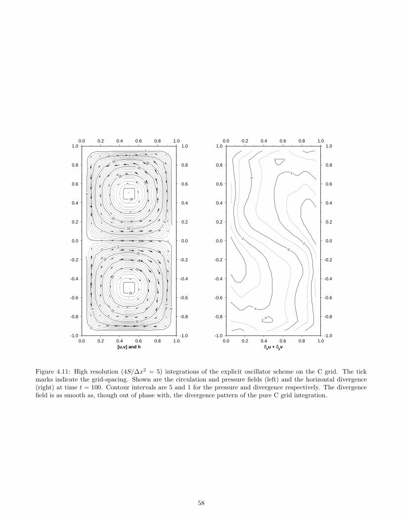
-25

-20

-20

-15

-15

-10

-10

-10

-5

-5

-5

0

0

0

0

0

5

5

5

10

10

10 15

15

20

20

25

-1.0

-0.8

-0.6

-0.4

-0.2

0.0

0.2

0.4

0.6

0.8

1.0

-1.0

-0.8

-0.6

-0.4

-0.2

0.0

0.2

0.4

0.6

0.8

1.0

0.0 0.2 0.4 0.6 0.8 1.0

0.0 0.2 0.4 0.6 0.8 1.0

[u,v] and h

-1

-1

-1

0

0

1

1

1

-1.0

-0.8

-0.6

-0.4

-0.2

0.0

0.2

0.4

0.6

0.8

1.0

-1.0

-0.8

-0.6

-0.4

-0.2

0.0

0.2

0.4

0.6

0.8

1.0

0.0 0.2 0.4 0.6 0.8 1.0

0.0 0.2 0.4 0.6 0.8 1.0

δxu + δyv

Figure 4.11: High resolution (4S/∆x2 = 5) integrations of the explicit oscillator scheme on the C grid. The tickmarks indicate the grid-spacing. Shown are the circulation and pressure fields (left) and the horizontal divergence(right) at time t = 100. Contour intervals are 5 and 1 for the pressure and divergence respectively. The divergencefield is as smooth as, though out of phase with, the divergence pattern of the pure C grid integration.

58

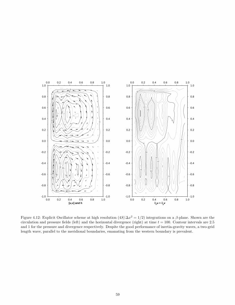
-20-2

0 -15 -1

5

-15

-10

-10

-10

-5-5

-5

0

0

0

0

5

5

5

10

1010

15

15

15

20

20

-1.0

-0.8

-0.6

-0.4

-0.2

0.0

0.2

0.4

0.6

0.8

1.0

-1.0

-0.8

-0.6

-0.4

-0.2

0.0

0.2

0.4

0.6

0.8

1.0

0.0 0.2 0.4 0.6 0.8 1.0

0.0 0.2 0.4 0.6 0.8 1.0

[u,v] and h

-5 -5

0

0

0

0

0

0

0

0

0

0

5

5

5

-1.0

-0.8

-0.6

-0.4

-0.2

0.0

0.2

0.4

0.6

0.8

1.0

-1.0

-0.8

-0.6

-0.4

-0.2

0.0

0.2

0.4

0.6

0.8

1.0

0.0 0.2 0.4 0.6 0.8 1.0

0.0 0.2 0.4 0.6 0.8 1.0

δxu + δyv

Figure 4.12: Explicit Oscillator scheme at high resolution (4S/∆x2 = 1/2) integrations on a β-plane. Shown are thecirculation and pressure fields (left) and the horizontal divergence (right) at time t = 100. Contour intervals are 2.5and 1 for the pressure and divergence respectively. Despite the good performance of inertia-gravity waves, a two-gridlength wave, parallel to the meridional boundaries, emanating from the western boundary is prevalent.

59

4.7 Summary

The GCM suffered from grid-scale noise when the Rossby radius of deformation was not resolved. An analysis of thebehavior of inertia-gravity waves in numerical models led to an understanding of the origin of the noise.

An alternative “oscillator” formulation of the momentum equations was proposed for implementation on theC grid. When compared with the solutions from the B and normal C grids, the scheme appears to successfullyrepresent the short inertia-gravity waves on the f plane. However, in the presence of a planetary vorticity gradient,the approach fails to represent Rossby waves adequately.

60

Chapter 5

Numerical Representation of RossbyWaves and the Cd scheme

Using the methods that were employed to understand inertia-gravity waves on numerical grids, the behaviour ofRossby waves can also be analysed. Rossby waves are a consequence of the Taylor-Proudman theorem and thegeometry of the earth1. Motions of sufficiently large scale can “feel” the variation in the Coriolis parameter. Becauseof the longer spatial scales, the time scales involved are typically longer than the rotation period of the earth.

The following section develops shallow water theory further to study the Rossby wave mode of motion. Theequivalent discrete analysis is then applied to grids studied in the previous chapter. Inspired by the “explicitoscillator” scheme developed for inertia-gravity waves, a new approach (the Cd scheme) is described that also treatsRossby waves with fidelity. The new scheme is analysed, tested and compared to the standard models. Finally, it isimplemented in the GCM and its performance evaluated.

5.1 Rossby Waves

In chapter 4, the shallow water equations were derived assuming that the horizontal scale of motion was small enoughthat variations in the Coriolis parameter could be assumed negligible, β 1. On the basin scale, this assumptionmust be relaxed. Further, the time-scale associated with these large spatial scales is much longer than the rotationperiod, 1

foT 1.

Allowing the variation in Coriolis parameter introduces Rossby waves into the model. The flow to the first twoorders in some arbitrary small parameter, ε, can be written:

u = uo + εu1+O(ε2) (5.1)

Substituting into the shallow water equations 4.12 and keeping only the order one terms yields:

ˆk ∧ uo + ∇h = 0 (5.2a)

S∇.uo = 0 (5.2b)

which are self consistent equations describing a quasi-geostrophic flow. The difference between a quasi-geostrophicmodel and a geostrophic model is that a reference Coriolis parameter is used in quasi-geostrophy, rather than thelocal value, in defining the geostrophic flow.

Defining the zeroth order flow by 5.2 and then substituting back into the shallow water equations and retainingall terms of order 1

foT, Ro, β and ε yields:

1

foT

∂

∂tuo + εk ∧ u

1+ βyk ∧ uo = 0 (5.3a)

1

foT

∂

∂th+ εS∇.U

1= 0 (5.3b)

which describe the slow evolution of the quasi-geostrophic flow in the presence of β. The ageostrophic componentof velocity can be eliminated by taking the curl of the momentum equation to form the vorticity equation and

1Strictly speaking, Rossby waves propagate in a Potential Vorticity gradient which does not necessarily require β.

61

substituting from the continuity equation:

1

foT

∂

∂tζo + βvo −

1

foT

1

S

∂

∂th = 0 (5.4)

The vorticity of the quasi-geostrophic flow can be written ζo = ∇2h and so equation 5.4 can be written in terms

of one variable, yielding the potential vorticity equation:

1

foT

∂

∂t∇

2h+ β∂

∂xh− 1

foT

1

S

∂

∂th = 0 (5.5)

The picture of this mode then, is one of a flow field in quasi-geostrophic equilibrium with the pressure gradients(the zeroth order balance), and a slowly evolving pressure field (the first order balance). The dispersion relation forlinear plane Rossby waves is obtained directly from 5.5:

ω =−βSk

1 + S(k2 + l2)(5.6)

Notice that the denominator takes the form of the square of the inertia-gravity wave frequency. The non-dimensional2 frequency is plotted as the first surface in figures 5.1 and 5.2. The β effect is the cause of the anisotropicpropagation.

The phase velocity:(

ω/kω/l

)

=βS

1 + S(k2 + l2)

(

−1−k/l

)

(5.7)

is always pointed towards the west with a maximum westward velocity of εβS (in dimensional units cφmax = βL2D

).The phase velocity behaves as 1/f 2 being larger near the equator than at the poles.

The group velocity:(

∂ω∂k∂ω∂l

)

=βS

(1 + S(k2 + l2))2

(

k2 − l2 − 1S

2klS

)

(5.8)

can be directed either eastward or westward depending on the sign of k2−l2−1/S. For short zonal waves k2 > l2+1/S,the group velocity has an eastward component whilst for long zonal waves k2 < l2 + 1, the zonal group velocity iswestward. Thus, whilst all wave fronts propagate westward, only long waves transmit energy westward. Short wavestransmit energy eastward. This anisotropy is one interpretation of the phenomena of western boundary intensification[Ped79].

The turning point in zonal group speed ( ∂ω∂k = 0) occurs at Sk2 = 1 + Sl2. The maximum frequency thus occurs

at l = 0, k = 1/√S with a frequency β

√S/2. In dimensional units this is a maximum frequency of βL

D/2 and is

typically of the order of a few cycles per month.

5.2 Finite-differenced Rossby waves

The quasi-geostrophic scaling applied in the previous section to obtain the Rossby wave mode of motion can be appliedto the finite difference models. The analysis (see Fox-Rabinovitz [FR91] and Wajsowicz [Waj86]) is summarised asfollows.

For the A grid:

Geostrophic: vg = δxhx

ug = −δyhy

(5.9a)

PV equation:∂

∂t(δxxh

xx+ δyyh

yy − 1

Sh) + β(δxh

xyy − ∆y2

4δxyyh

x) = 0 (5.9b)

Dispersion: ω =εβSskck(c

2l + ∆y2s2l /4)

1 + S(s2kc2k + s2l c

2l )

(5.9c)

For the B grid:

Geostrophic: vg = δxhy

ug = −δyhx

(5.10a)

PV equation:∂

∂t(δxxh

yy+ δyyh

xx − 1

Sh) + βδxh

x= 0 (5.10b)

Dispersion: ω =εβSskck

1 + S(s2kc2l + s2l c

2k)

(5.10c)

2Time was non-dimensionalised with respect to f in chapter 4.

62

For the C grid:

Geostrophic: vgxy = δxh ug

xy = −δyh (5.11a)

PV equation:∂

∂t(δxxh+ δyyh− 1

Shxxyy

) + βδxhxyy

= 0 (5.11b)

Dispersion: ω =εβSskckc

2l

c2kc2l + S(s2k + s2l )

(5.11c)

For the D grid:

Geostrophic: vg = δxh ug = −δyh (5.12a)

PV equation:∂


Sh) + βδxh

xyy= 0 (5.12b)


2l

1 + S(s2k + s2l )(5.12c)

For the explicit oscillator scheme on a C grid:

Geostrophic: vg = δxhxy

ug = −δyhxy

(5.13a)

PV equation:∂


Sh) + βδxh

xyy= 0 (5.13b)


2l

1 + S(s2k + s2l )(5.13c)

It is interesting to note that the explicit oscillator scheme, despite a very different representation of the physics,exhibits the same Rossby wave dispersion as the D grid.

One observation about the dispersion relations, as written, is that the denominator of the expressions for thefrequency take the form of the dispersion relation of the inertia-gravity waves for the respective grid. Therefore, thedenominator is likely to have some artificial zero points creating singularities in the frequency. In fact, this does notbecome a problem since wherever a singularity might occur, the numerator has an artificial zero that vanishes morerapidly.

Figures 5.1 and 5.2 show the discrete dispersion relations plotted for high and low wave resolutions respectively.Included in the the diagram is the dispersion relation pertaining to the Eliassen time-staggered grid that will bedescribed later in this chapter.

Both the high and low resolution dispersion relation for the A grid have artificial turning points. Simply put,the shorter A grid Rossby waves bear no resemblance in dispersion properties to the continuum. Of the otherhigh resolution dispersion relations (figure 5.1) only the B grid exhibits a qualitative difference to the continuum.This takes the form of artificially fast zonal group speed for long meridional waves. The B, C and D grids havezero frequencies for zonal grid length waves but since the continuum has very low frequencies here, the qualitativebehaviour is unchanged.

As was the case for the inertia-gravity waves, the dispersion relations for the different grids dramatically changetheir behaviour as one moves from high to low resolution. Figure 5.2 shows the frequency for short zonal waves.None of the grids reproduce the behaviour of the continuum plot properly.

All the models except the B grid have artificially high meridional group speeds. This means that the models areable to meridionally redistribute energy in an artificial manner.

One point in favour of the C grid at low resolution is that for short meridional waves, the zonal group speed ismuch closer to the continuum than the B grid (i.e. the artificial turning point is at a shorter wave number on theC grid than on the B grid). Indeed, the B grid has the wrong sign for several of the shortest zonal wave numberswhilst the C grid is in error for only the shortest. This has implications for western boundary intensification in themodels. If waves that are longer than the grid-scale can transmit energy eastward then the western boundary layermay be artificially wider as a result.

It is interesting to note that for the D grid, despite a very poor representation of inertia-gravity waves, the Rossbywaves seem to be well represented. This is due to the natural geostrophic balance that has no spatial averaging in it.

63

−1 0 10

0.5

1

−0.050

0.05

mnw

Continuum

−1 0 10

0.5

1

−0.050

0.05

mn

w

A grid

−1 0 10

0.5

1

−0.050

0.05

mn

w

B grid

−1 0 10

0.5

1

−0.050

0.05

mn

w

C grid

−1 0 10

0.5

1

−0.050

0.05

mn

w

D grid

−1 0 10

0.5

1

−0.050

0.05

mn

wDD grid

Figure 5.1: Rossby wave dispersion relations for the continuum and high resolution finite difference models(A,B,C,D,DD) with a wave resolution of 2

√S/∆x = 3.

5.3 Time staggered grids

It is should be clear from the results of using the explicit oscillator scheme that both classes of discrete wave motionneed to be taken into account; mis-representation of the inertia-gravity waves generates erroneous divergence patternson a short time scale whilst mis-representation of Rossby waves generates spurious standing waves on a much longertime scale.

Of the gridding schemes discussed so far, none of them satisfactorily meets both requirements at all wave reso-lutions. To devise a scheme that can achieve this goal, one might begin by considering one that performs well atjust one scale. Here, the C grid performs particularly well at high wave resolution and the B grid is perhaps to befavoured at low resolution (this decision is based upon the accurate meridional propagation of energy rather than thescale of the western boundary current). However, since the non-hydrostatic physics in the GCM is most naturallydescribed on a C grid, the following discussion will concentrate upon the C grid structure.

There are in fact many gridding schemes that can be introduced when more than one time step is used in thetime-stepping algorithm. This involves staggering variables not only in space but also in time. This was alreadyan implicit feature of the single time step schemes of the previous B and C grid models. The pressure variable wasstaggered in time with the velocity variables allowing second order finite differencing in both time and space for thegravity waves.

Five gridding schemes derived from the five Arakawa grids were described by Eliassen [MA76, FR91]. The methodshifts the grid diagonally at alternating time-steps. Figure 5.3 shows the three dimensional distribution of variablesin space and time for the five grids. The primed notation indicates that the grid is shifted diagonally in space fromthe unprimed position. The models are described as follows:

64

−1 0 10

0.5

1−5

05

x 10−3

mnw

Continuum

−1 0 10

0.5

1−5

05

x 10−3

mn

w

A grid

−1 0 10

0.5

1−5

05

x 10−3

mn

w

B grid

−1 0 10

0.5

1−5

05

x 10−3

mn

w

C grid

−1 0 10

0.5

1−5

05

x 10−3

mn

w

D grid

−1 0 10

0.5

1−5

05

x 10−3

mn

wDD grid

Figure 5.2: Rossby wave dispersion relations for the continuum and low resolution finite difference models(A,B,C,D,DD) with a wave resolution of 2

√S/∆x = 1/3.

Scheme AA’:

δtut − vxy + δxh

y= 0 (5.14a)

δtvt + uxy + δyh

x= 0 (5.14b)

δtht+ S(δxu

y + δyvx) = 0 (5.14c)

IG dispersion: ω2 = c2kc2l + S(s2kc

2l + s2l c

2k) (5.14d)

Scheme BB’:

δtut − vxy + δxh

x= 0 (5.15a)

δtvt + uxy + δyh

y= 0 (5.15b)

δtht+ S(δxu

x + δyvy) = 0 (5.15c)

IG dispersion: ω2 = c2kc2l + S(s2kc

2k + s2l c

2l ) (5.15d)

Scheme CC’:

δtut − v + δxh

xy= 0 (5.16a)

δtvt + u+ δyh

xy= 0 (5.16b)

65

Auvh

A’uvh uvh

uvhuvh

Auvh

A’uvh uvh

uvhuvh

Buv uv

uvuvh

B’h

uvh

hh

Buv uv

uvuvh

B’h

uvh

hh

Cu u

vh

v

C’h

h h

hv v

u

u

Cu u

vh

v

C’h

h h

hv v

u

u

Dh

u

uv v

D’h

h h

hv

vu u

Dh

u

uv v

D’h

h h

hv

vu u

Eh

h

h h

h

uv

uvuvuv

E’uv

uv

uv uv

uvh

hh

h

Eh

h

h h

h

uv

uvuvuv

E’uv

uv

uv uv

uvh

hh

h

time

y

x

Figure 5.3: The Eliassen time horizontally staggered grids, AA’,BB’,CC’,DD’,EE’

δtht+ S(δxu

xy + δyvxy) = 0 (5.16c)

IG dispersion: ω2 = 1 + Sc2kc2l (s

2k + s2l ) (5.16d)

Scheme DD’:

δtut − v + δxh = 0 (5.17a)

δtvt + u+ δyh = 0 (5.17b)

δtht+ S(δxu+ δyv) = 0 (5.17c)

IG dispersion: ω2 = 1 + S(s2k + s2l ) (5.17d)

Again, the EE’ grid is a rotated and scaled (by√

2) version of the BB’ grid and so omitted. All the above modelsuse explicit evaluation of both Coriolis and pressure terms. The spatial interpolation of these terms can actually bereduced or even avoided by semi-implicit (centered over two time levels) evaluation. For example the Coriolis termsof the AA’ grid could replace the −xy with a −2t with no loss of efficiency or accuracy. Here, only the fully explicitmodels will be considered to allow an easy transfer of algorithms to more sophisticated models.

Before continuing with a closer look at these time staggered grids, there are a number of cautionary points:

• The storage requirements of the computer system can be as much as doubled because there is a duplication ofvariables.

• There is a duplication of physical boundary conditions.

• There is a tendency for the two alternating grids to decouple (in the manner of a leap-frog computationalmode); this can be alleviated by adding filtering terms.

The decoupling can be thought of as a consequence of the splitting of each of the natural modes of the system.So there might be two geostrophic modes and two pairs of inertia-gravity modes. The pair may look identical indispersion qualities but the reciprocal pairs are linearly independent.

The grid that draws our attention is the DD’ grid. No interpolation operators appear in the finite differenceequations and thus the inertia-gravity wave dispersion relation is the same as that of the explicit oscillator schemeof the previous chapter.

66

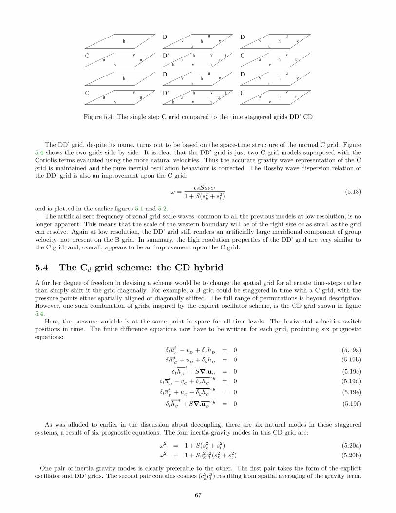
v

vu u

h

v

vu u

h

C

C

Dh

u

uv v

D’h

h h

hv

vu u

Dh

u

uv v

D’h

h h

hv

vu u

Dh

u

uv v

Cu u

vh

v

Dh

u

uv v

Cu u

vh

v

Figure 5.4: The single step C grid compared to the time staggered grids DD’ CD

The DD’ grid, despite its name, turns out to be based on the space-time structure of the normal C grid. Figure5.4 shows the two grids side by side. It is clear that the DD’ grid is just two C grid models superposed with theCoriolis terms evaluated using the more natural velocities. Thus the accurate gravity wave representation of the Cgrid is maintained and the pure inertial oscillation behaviour is corrected. The Rossby wave dispersion relation ofthe DD’ grid is also an improvement upon the C grid:

ω =εβSskcl

1 + S(s2k + s2l )(5.18)

and is plotted in the earlier figures 5.1 and 5.2.The artificial zero frequency of zonal grid-scale waves, common to all the previous models at low resolution, is no

longer apparent. This means that the scale of the western boundary will be of the right size or as small as the gridcan resolve. Again at low resolution, the DD’ grid still renders an artificially large meridional component of groupvelocity, not present on the B grid. In summary, the high resolution properties of the DD’ grid are very similar tothe C grid, and, overall, appears to be an improvement upon the C grid.

5.4 The Cd grid scheme: the CD hybrid

A further degree of freedom in devising a scheme would be to change the spatial grid for alternate time-steps ratherthan simply shift it the grid diagonally. For example, a B grid could be staggered in time with a C grid, with thepressure points either spatially aligned or diagonally shifted. The full range of permutations is beyond description.However, one such combination of grids, inspired by the explicit oscillator scheme, is the CD grid shown in figure5.4.

Here, the pressure variable is at the same point in space for all time levels. The horizontal velocities switchpositions in time. The finite difference equations now have to be written for each grid, producing six prognosticequations:

δtutC− v

D+ δxhD

= 0 (5.19a)

δtvtC

+ uD

+ δyhD= 0 (5.19b)

δthD

t+ S∇.u

C= 0 (5.19c)

δtutD− v

C+ δxhC

xy= 0 (5.19d)

δtvtD

+ uC

+ δyhC

xy= 0 (5.19e)

δthC

t+ S∇.u

D

xy = 0 (5.19f)

As was alluded to earlier in the discussion about decoupling, there are six natural modes in these staggeredsystems, a result of six prognostic equations. The four inertia-gravity modes in this CD grid are:

ω2 = 1 + S(s2k + s2l ) (5.20a)

ω2 = 1 + Sc2kc2l (s

2k + s2l ) (5.20b)

One pair of inertia-gravity modes is clearly preferable to the other. The first pair takes the form of the explicitoscillator and DD’ grids. The second pair contains cosines (c2kc

2l ) resulting from spatial averaging of the gravity term.

67

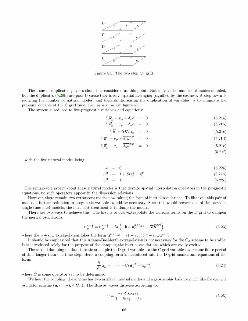
Cu u

v

v

Cu u

v

v

hu

uv v

D

hu

uv v

D

Figure 5.5: The two step Cd grid.

The issue of duplicated physics should be considered at this point. Not only is the number of modes doubled,but the duplicates (5.20b) are poor because they involve spatial averaging (signified by the cosines). A step towardsreducing the number of natural modes, and towards decreasing the duplication of variables, is to eliminate thepressure variable at the C grid time level, as is shown in figure 5.5.

The system is reduced to five prognostic variables and equations:

δtutC− v

D+ δxh = 0 (5.21a)

δtvtC

+ uD

+ δyh = 0 (5.21b)

δtht+ S∇.u

C= 0 (5.21c)

δtutD− v

C+ δxh

xyt= 0 (5.21d)

δtvtD

+ uC

+ δyhxyt

= 0 (5.21e)

(5.21f)

with the five natural modes being:

ω = 0 (5.22a)

ω2 = 1 + S(s2k + s2l ) (5.22b)

ω2 = 1 (5.22c)

The remarkable aspect about these natural modes is that despite spatial interpolation operators in the prognosticequations, no such operators appear in the dispersion relations.

However, there remain two extraneous modes now taking the form of inertial oscillations. To filter out this pair ofmodes, a further reduction in prognostic variables would be necessary. Since this would recover one of the previoussingle time level models, the next best treatment is to damp the modes.

There are two ways to achieve this. The first is to over-extrapolate the Coriolis terms on the D grid to dampenthe inertial oscillations.

un+ 12

D= un−

12

D+ ∆t

(

−k ∧ un+ε

ABC − ∇h

xyt)

(5.23)

where the n+ εAB

extrapolation takes the form un+εAB = (1 + ε

AB)Un − ε

ABun−1.

It should be emphasized that this Adams-Bashforth extrapolation is not necessary for the Cd scheme to be stable.It is introduced solely for the purpose of the damping the inertial oscillations which are easily excited.

The second damping method is to tie or couple the D grid variables to the C grid variables over some finite periodof time longer than one time step. Here, a coupling term is introduced into the D grid momentum equations of theform:

∂

∂tu

D+ . . . = −C(u

D

t − uC

xy) (5.24)

where C is some operator yet to be determined.Without the coupling, the scheme has two artificial inertial modes and a geostrophic balance much like the explicit

oscillator scheme (uC = −ˆk ∧ ∇h). The Rossby waves disperse according to:

ω =−εβSskckc2k

1 + S(s2k + s2l )(5.25)

68

which is the same as for the D grid and explicit oscillator scheme. In fact, on closer examination, the scheme is justthe integral form of the second order equations employed in devising the explicit oscillator scheme.

If one fully relaxes the D grid velocities to the C grid in one time step, then they become equal, by definition,to the spatial average of the C grid velocities for all time. In this limit, the scheme becomes the normal single timelevel C grid.

For the case of coupling on a time scale longer than the inertial period but shorter than the period of the fastestRossby wave (εβ

√S/2 < λ < 1), the inertia-gravity waves will be relatively unaffected since the motion is on a much

shorter time-scale than the relaxation. So the good short time scale performance of the explicit oscillator scheme isreproduced here. On time-scales longer than the relaxation, the D grid velocities are fully relaxed to the interpolatedC grid values so the geostrophic balance takes the form of the C grid: uxy = −k ∧ ∇h.

This would yield the optimum attributes of the two inherent grids. It then remains to determine the form thatthe coupling operator should take.

5.5 Determining the optimal coupling

Damped inertia-gravity waves are described by the continuous equations:

∂

∂tu + k ∧ u + S∇h = −F (u) (5.26a)

∂

∂th+ ∇ · u = −H(h) (5.26b)

where D and H are dissipative operators, yet to be specified. The corresponding divergence equation is:

[

(F +∂

∂t)2 + 1 − S(H +

∂

∂t)∇2

]

∇ · u = 0 (5.27)

The finite difference equations using the Cd scheme, including the coupling term C(uD− uxy

C, are:

∂

∂tu

C+ k ∧ u

D+ S∇h = −F (u

C) (5.28a)

∂

∂tu

D+ k ∧ u

C+ S∇h

xy= −F (uxy

C) − C(u

D− uxy

C) (5.28b)

∂

∂th+ ∇ · u

C= −H(h) (5.28c)

where C is still arbitrary.The divergence (∇ · u

C) equation, that governs the dispersion of the discrete inertia-gravity waves, is:

[

(F +∂

∂t)(C +

∂

∂t) + 1 − S(H +

∂

∂t)∇2

]

∇ · uC

+ (F − C)ζxy

C= 0 (5.29)

which has a new term involving vorticity on the C grid. This term vanishes only if:

C = F (5.30)

which indicates that the coupling should take the form of the dissipation in the momentum equations. The divergencewave equation then looks very much like the continuous system with no interpolation operators.

The natural modes of the system on an f-plane are given by:

(

(F +∂

∂t)2 + 1

) (

(F +∂

∂t)2 + 1

)

(H +∂

∂t) − (F +

∂

∂t)S∇

2

h = 0 (5.31)

The first factor gives rise to the inertial oscillations, now damped both by the explicit dissipation and thatimplied in the Adams-Bashforth time-stepping. The second factor corresponds to the damped inertia-gravity wavescorresponding to 5.27. There are no spatial interpolation operators here, so the inertia-gravity waves should not haveany artificial signs in phase and group speed.

69

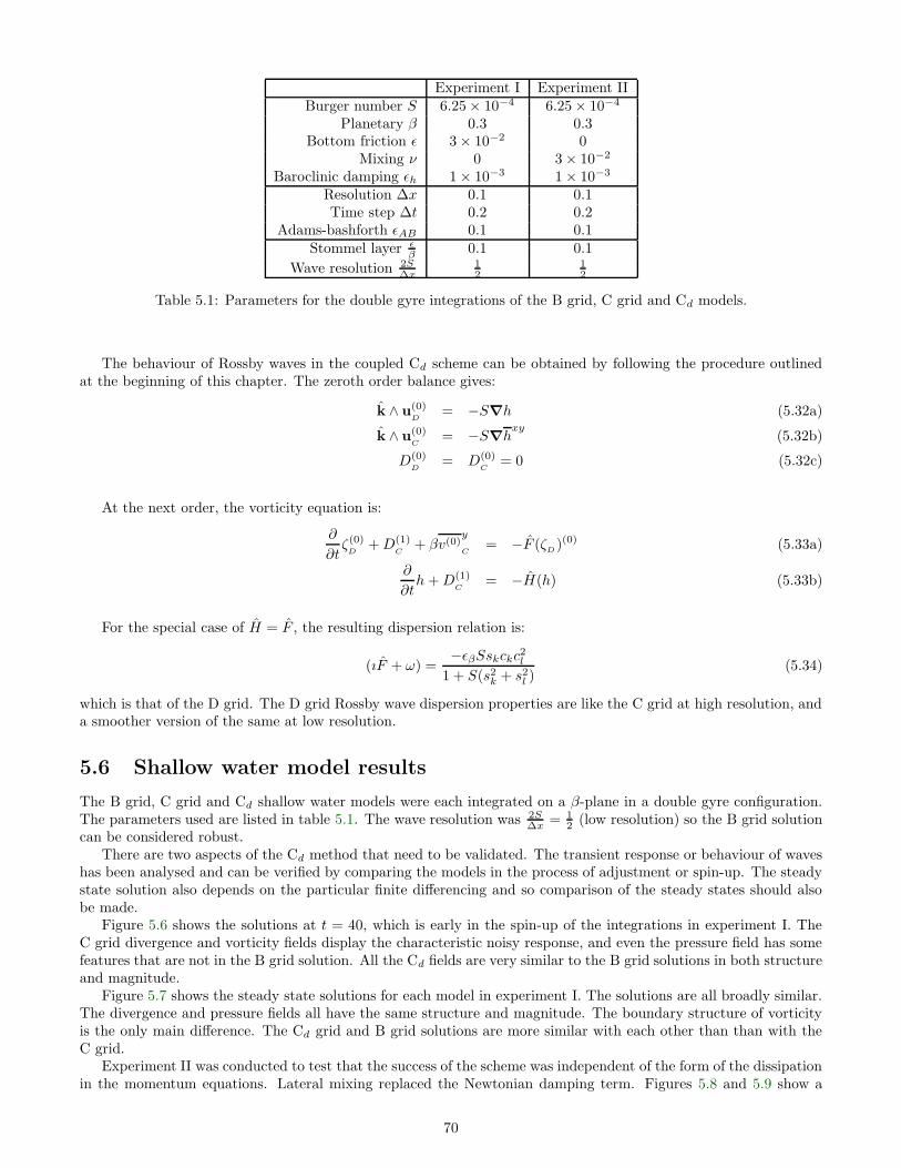
Experiment I Experiment IIBurger number S 6.25× 10−4 6.25× 10−4

Planetary β 0.3 0.3Bottom friction ε 3 × 10−2 0

Mixing ν 0 3 × 10−2

Baroclinic damping εh 1 × 10−3 1 × 10−3

Resolution ∆x 0.1 0.1Time step ∆t 0.2 0.2

Adams-bashforth εAB 0.1 0.1Stommel layer ε

β 0.1 0.1

Wave resolution 2S∆x

12

12

Table 5.1: Parameters for the double gyre integrations of the B grid, C grid and Cd models.

The behaviour of Rossby waves in the coupled Cd scheme can be obtained by following the procedure outlinedat the beginning of this chapter. The zeroth order balance gives:

k ∧ u(0)D

= −S∇h (5.32a)

k ∧ u(0)C

= −S∇hxy

(5.32b)

D(0)D

= D(0)C

= 0 (5.32c)

At the next order, the vorticity equation is:

∂

∂tζ(0)

D+D(1)

C+ βv(0)

y

C= −F (ζ

D)(0) (5.33a)

∂

∂th+D(1)

C= −H(h) (5.33b)

For the special case of H = F , the resulting dispersion relation is:

(ıF + ω) =−εβSskckc2l

1 + S(s2k + s2l )(5.34)

which is that of the D grid. The D grid Rossby wave dispersion properties are like the C grid at high resolution, anda smoother version of the same at low resolution.

5.6 Shallow water model results

The B grid, C grid and Cd shallow water models were each integrated on a β-plane in a double gyre configuration.The parameters used are listed in table 5.1. The wave resolution was 2S

∆x = 12 (low resolution) so the B grid solution

can be considered robust.There are two aspects of the Cd method that need to be validated. The transient response or behaviour of waves

has been analysed and can be verified by comparing the models in the process of adjustment or spin-up. The steadystate solution also depends on the particular finite differencing and so comparison of the steady states should alsobe made.

Figure 5.6 shows the solutions at t = 40, which is early in the spin-up of the integrations in experiment I. TheC grid divergence and vorticity fields display the characteristic noisy response, and even the pressure field has somefeatures that are not in the B grid solution. All the Cd fields are very similar to the B grid solutions in both structureand magnitude.

Figure 5.7 shows the steady state solutions for each model in experiment I. The solutions are all broadly similar.The divergence and pressure fields all have the same structure and magnitude. The boundary structure of vorticityis the only main difference. The Cd grid and B grid solutions are more similar with each other than than with theC grid.

Experiment II was conducted to test that the success of the scheme was independent of the form of the dissipationin the momentum equations. Lateral mixing replaced the Newtonian damping term. Figures 5.8 and 5.9 show a

70

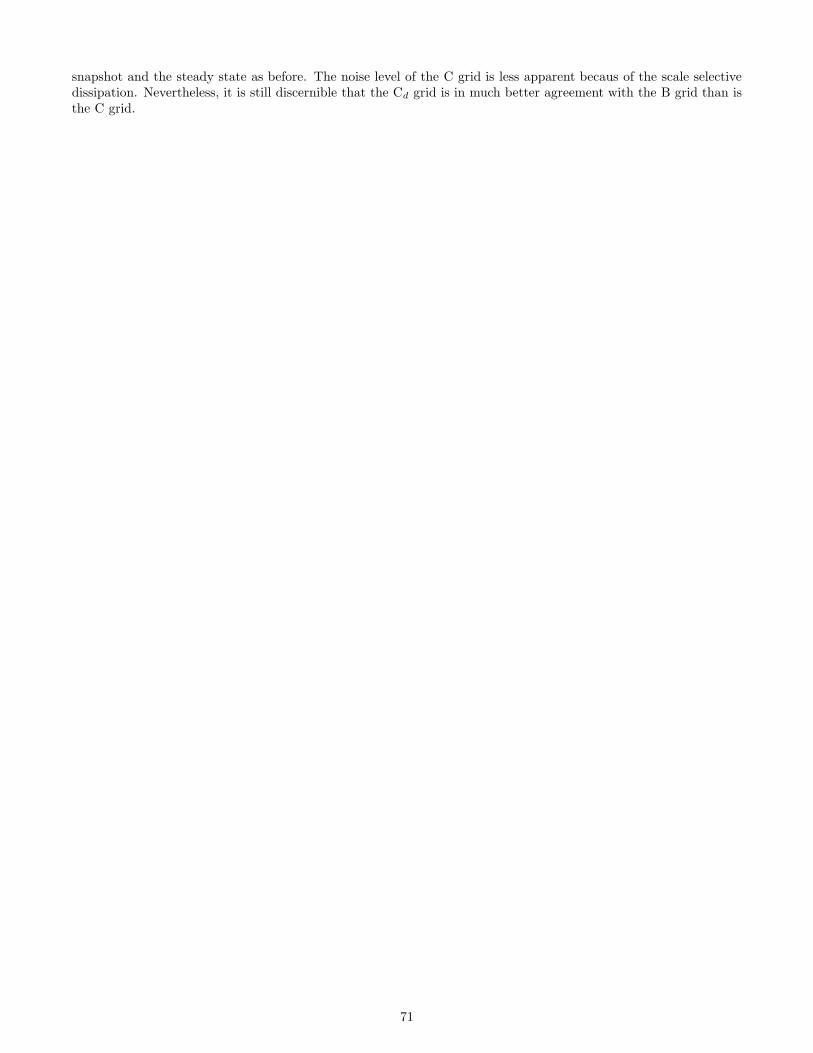
snapshot and the steady state as before. The noise level of the C grid is less apparent becaus of the scale selectivedissipation. Nevertheless, it is still discernible that the Cd grid is in much better agreement with the B grid than isthe C grid.

71

(B)

0.2 0.4 0.6 0.8

−0.8

−0.6

−0.4

−0.2

0

0.2

0.4

0.6

0.8

X

Yh

−10

−10

−10

0

0

0

0

0

10

0.2 0.4 0.6 0.8

−0.8

−0.6

−0.4

−0.2

0

0.2

0.4

0.6

0.8

X

Y

D

−15

−10

−10

−10

−5

−5

−5

−5

−5

0

0

0

0

0

5

5

5

5

510

10

ζ

0.2 0.4 0.6 0.8

−0.8

−0.6

−0.4

−0.2

0

0.2

0.4

0.6

0.8

X

Y

−80−60−60

−40

−40

−40

−40

−20

−20

−20

−20

−20

0

000

0

0

20

20

20

20

20

20

60

(C)

0.2 0.4 0.6 0.8

−0.8

−0.6

−0.4

−0.2

0

0.2

0.4

0.6

0.8

X

Y

h

−20

−10

−10

−10−10

−10

−10

0

0

0

0

0

10

10

10

10

10

0.2 0.4 0.6 0.8

−0.8

−0.6

−0.4

−0.2

0

0.2

0.4

0.6

0.8

X

Y

D

−20

−15

−15

−15

−10

−10

−10

−5

−5

−5

−5

0

00

0

05

55

55

10

10

10

10

15

15

20

ζ

0.2 0.4 0.6 0.8

−0.8

−0.6

−0.4

−0.2

0

0.2

0.4

0.6

0.8

X

Y

−200

−180

−160

−160

−140

−140

−120

−100

−100

−80−60

−60

−40

−40

−40

−40

−40

−20

−20

−20−20

−20

0

0

00

0

00

0

0

020

20

2020

20

40

40

40

60

60

80

80

100

100

120

120

140

140

200

(Cd )

0.2 0.4 0.6 0.8

−0.8

−0.6

−0.4

−0.2

0

0.2

0.4

0.6

0.8

X

Y

h−10

−10

−10

0

0

0

0

0

010

10

0.2 0.4 0.6 0.8

−0.8

−0.6

−0.4

−0.2

0

0.2

0.4

0.6

0.8

X

Y

D

−15

−10

−10

−10

−5

−5

−5

−5

−5

0

0

0

0

0

5

5

5

5

510

10

10

15

15

ζ

0.2 0.4 0.6 0.8

−0.8

−0.6

−0.4

−0.2

0

0.2

0.4

0.6

0.8

X

Y

−40

−20

−20

−20

0

0

20

20

20

Figure 5.6: Surface elevation h with velocity vectors, vorticity ζ and divergence D for the three models B, C and Cd

at t = 40 in experiment I. The solutions are in the early stage of adjustment. Note the noise in the divergence fieldof the C grid.

72

(B)

0.2 0.4 0.6 0.8

−0.8

−0.6

−0.4

−0.2

0

0.2

0.4

0.6

0.8

X

Yh

−250

−200

−150

−150

−100

−100

−100−50

−50

−500

0

0

50

50

50

100

100

150

200

250

0.2 0.4 0.6 0.8

−0.8

−0.6

−0.4

−0.2

0

0.2

0.4

0.6

0.8

X

Y

D

−10

−5

−5

0

0

0

5

5 10

ζ

0.2 0.4 0.6 0.8

−0.8

−0.6

−0.4

−0.2

0

0.2

0.4

0.6

0.8

X

Y

−350 −300−250

−200

−150

−150

−150

−100

−100

−100

−50

−50

−50

0

0

0

00

0

50 50

50

50100

100

100

150

150200

250

300

(C)

0.2 0.4 0.6 0.8

−0.8

−0.6

−0.4

−0.2

0

0.2

0.4

0.6

0.8

X

Y

h

−200

−200

−150

−100

−100−50

−50

−500

50

100

150

150

200

250

300

0.2 0.4 0.6 0.8

−0.8

−0.6

−0.4

−0.2

0

0.2

0.4

0.6

0.8

X

Y

D

−10 −5

0

0

5

5

10

ζ

0.2 0.4 0.6 0.8

−0.8

−0.6

−0.4

−0.2

0

0.2

0.4

0.6

0.8

X

Y

−150

−100

−50

0

0

50

100

150

(Cd )

0.2 0.4 0.6 0.8

−0.8

−0.6

−0.4

−0.2

0

0.2

0.4

0.6

0.8

X

Y

h

−200 −1

50

−100

−100−50

−50

−50

0

0

0

50

50

50

50

100

100

150

150

200

250

0.2 0.4 0.6 0.8

−0.8

−0.6

−0.4

−0.2

0

0.2

0.4

0.6

0.8

X

Y

D

−10

−5

−50

0

0

5

5

10

ζ

0.2 0.4 0.6 0.8

−0.8

−0.6

−0.4

−0.2

0

0.2

0.4

0.6

0.8

X

Y

−250

−200

−150

−150

−100

−50

−50

−50

0

0

0

0

050

50

50

100

100150


at t = 5000 in experiment I. The solutions are the steady state. The C grid vorticity field has a different boundarystructure to the B and Cd grid solutions.

73

(B)

0.2 0.4 0.6 0.8

−0.8

−0.6

−0.4

−0.2

0

0.2

0.4

0.6

0.8

X

Yh

−10

−10

−10

0

0

0

0

0

10

20

0.2 0.4 0.6 0.8

−0.8

−0.6

−0.4

−0.2

0

0.2

0.4

0.6

0.8

X

Y

D

−15

−10

−10

−10

−5

−5

−5

−5

0

0

0

0

0

5

5

5

5

5

10

10

15

ζ

0.2 0.4 0.6 0.8

−0.8

−0.6

−0.4

−0.2

0

0.2

0.4

0.6

0.8

X

Y

−20

−20

−20

−20

0

0

0

0

0

0

20

20

(C)

0.2 0.4 0.6 0.8

−0.8

−0.6

−0.4

−0.2

0

0.2

0.4

0.6

0.8

X

Y

h

−20

−10

−10

−10

−10

0

0

0

0

0

10

10

10

20

0.2 0.4 0.6 0.8

−0.8

−0.6

−0.4

−0.2

0

0.2

0.4

0.6

0.8

X

Y

D

−20−15

−15

−10

−10

−10

−10

−5

−5

−5

−5

0

0

0

05

5

5

5

10

10

10

15

15

15

2025

ζ

0.2 0.4 0.6 0.8

−0.8

−0.6

−0.4

−0.2

0

0.2

0.4

0.6

0.8

X

Y

−60

−40

−40

−20

0

0

20

40

40

60

(Cd )

0.2 0.4 0.6 0.8

−0.8

−0.6

−0.4

−0.2

0

0.2

0.4

0.6

0.8

X

Y

h

−10

−10

−10

0

0

0

0

0

10

0.2 0.4 0.6 0.8

−0.8

−0.6

−0.4

−0.2

0

0.2

0.4

0.6

0.8

X

Y

D

−15

−10

−10

−10

−10

−5

−5

−5

−5

0

0

0

0

5

5

5

5

10

10

10

15

ζ

0.2 0.4 0.6 0.8

−0.8

−0.6

−0.4

−0.2

0

0.2

0.4

0.6

0.8

X

Y

−20−20

0

0

0

0

Figure 5.8: Surface elevation h with velocity vectors, vorticity ζ and divergence D for the three models B, C andCd at t = 40 in experiment II. The solutions are in the early stage of adjustment. Note the substantial difference inpattern and magnitude of the vorticity field on the C grid.

74

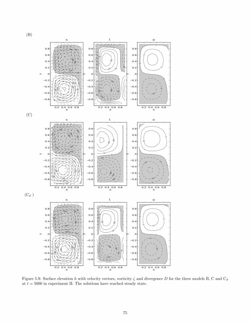
(B)

0.2 0.4 0.6 0.8

−0.8

−0.6

−0.4

−0.2

0

0.2

0.4

0.6

0.8

X

Yh

−200

−150

−100

−100

−50

−50

0

0

0

50

50

100

100

150

150 200

0.2 0.4 0.6 0.8

−0.8

−0.6

−0.4

−0.2

0

0.2

0.4

0.6

0.8

X

Y

D

−10

−50

0

0

5

5

ζ

0.2 0.4 0.6 0.8

−0.8

−0.6

−0.4

−0.2

0

0.2

0.4

0.6

0.8

X

Y

−200

−100

−100

−50

−50 −50

0

0

0

0

0

50

50

5010

0

100

150

(C)

0.2 0.4 0.6 0.8

−0.8

−0.6

−0.4

−0.2

0

0.2

0.4

0.6

0.8

X

Y

h

−300−250

−200

−200

−150

−150

−100

−100

−50

−500

050

50

100

100

150

150

200250

300

0.2 0.4 0.6 0.8

−0.8

−0.6

−0.4

−0.2

0

0.2

0.4

0.6

0.8

X

Y

D

−10

−10−5

−5

05

5

10

ζ

0.2 0.4 0.6 0.8

−0.8

−0.6

−0.4

−0.2

0

0.2

0.4

0.6

0.8

X

Y

−200

−150

−100

−50

050

100

150

(Cd )

0.2 0.4 0.6 0.8

−0.8

−0.6

−0.4

−0.2

0

0.2

0.4

0.6

0.8

X

Y

h

−250

−200

−150

−100

−100

−50

−50

−50

0

0

0

50

50

100

100

150

150

200200 300

0.2 0.4 0.6 0.8

−0.8

−0.6

−0.4

−0.2

0

0.2

0.4

0.6

0.8

X

Y

D

−10

−5

−5

0

0

0

5

5

10

ζ

0.2 0.4 0.6 0.8

−0.8

−0.6

−0.4

−0.2

0

0.2

0.4

0.6

0.8

X

Y

−200

−150

−100

−50

0

0

0

0

0

50

50

50

100

150


at t = 5000 in experiment II. The solutions have reached steady state.

75

5.7 Implementation of the Cd scheme in the GCM

The complete procedure applied to a baroclinic model will now be described. All terms excluding the pressuregradient and Coriolis terms are collected into a vector G.

Define uC

to fall at the integer time levels (n−1, n, n+1) and define the pressure variable to fall at the half-integerlevels (n−1

2 , n+12 ) as before. Now introduce new horizontal velocities u

Dto fall at the same half integer time levels

as the pressure but are positioned in the D grid configuration.At the beginning of the time-step to step forward for the n+1 C grid velocities, all variables at time n−1 1

2 , n−1,n−1

2 and n are known.u

Dat n+1

2 is estimated by writing a centered single level time-stepping scheme in terms of uC

and G at time leveln. Note that the pressure gradient terms have to be extrapolated forward in time in an analogous manner to thequasi-second order method AB2 (to avoid an implicit evaluation of the pressure at this stage). The zonal componentof the D grid momentum equations is:

u(n+ 1

2)

D

∆t=u

(n− 12)

D

∆t+G

(n)u

xy

+1

∆xδx(

3

2+ ε

AB)P (n− 1

2) − (

1

2+ ε

AB)P (n−1 1

2)

xy

+fx((1 + ε

AB)v(n)

C− ε

ABv(n−1)

C) (5.35)

+F

(

uD− 1

2(u

(n)C + u

(n−1)C )

xy)

The operator F is the same as the dissipation operator used within the vector G.The C grid velocities are then found as in the conventional scheme except that now the Coriolis term is written

as the vector C:u(n+1)

C

∆t=u(n)

C

∆t+ (

3

2+ ε

AB)G(n)

u − (1

2+ ε

AB)G(n−1)

u +1

∆xδxP

(n+ 12) + Cu (5.36)

where Cu is defined:

Cu =

f( 32 + ε

AB)v

(n)C − ( 1

2 + εAB

)v(n−1)C

yx

if C grid is used

fxvn+ 1

2D if Cd grid is used

(5.37)

It should be apparent from this formulation that the D grid velocities only enter the model through the Coriolisterm and are not used anywhere else. Obviously, if the C grid evaluation of Coriolis is used then the D grid velocitiesare redundant and need not be stepped forward.

The North Pacific integration in chapter 3 was used as the context in which to discuss problems inherent in the‘C’ grid at coarse resolution. Figures 5.10 and 5.11 show the vertical velocity in the GCM for the same experimentbut with the Cd scheme implemented. They correspond to figures 3.9 and 3.10 that were dominated by grid lengthwaves in the unmodified C grid version of the model, just one month after the Cd scheme was switched off.

The scheme no longer allows grid scale noise to persist in the model. The major features of the Pacific circulation,such as the Kurishio and strong Equatorial upwelling, are unaffected by the scheme.

5.8 Discussion

Form of the Coupling During the development of the Cd scheme, it was not immediately realised that there was anoptimum form for the coupling operator. Instead, the simplest possible form of Newtonian relaxation (−λ(u

D−u

C

xy)was chosen. The relaxation time-scale was at first chosen using a somewhat subjective selection criteria. A connectionbetween the grid-scale dissipation rates and the optimum choice of λ was empirically established. The implicationsof using such a coupling were that:

• all modes, both horizontal and vertical, would ‘feel’ the same damping rate. This could produce smoother thanexpected flows, with slower currents.

• for a poorly chosen λ, some modes could be excessively dissipated or tend to become de-coupled. The formermanifests itself by smoothing the flow whilst the latter appears as a checker-board mode in the pressure field.

• there was an extra parameter for the model that had to be determined prior to integration.

All of these factors rendered this simple coupling method undesirable. The proposed method, of coupling using thedissipation operator, suffers from none of these problems.

76

140 160 180 200 220 240 260 280−30

−20

−10

0

10

20

30

40

50

60

Longitude

Latit

ude

Figure 5.10: Vertical velocity at the base of the top layer in the model after one month. Contour interval is 0.01 mms−1.

140 160 180 200 220 240 260 280−30

−20

−10

0

10

20

30

40

50

60

Longitude

Latit

ude

0

0

0

0

0

0

0

0

0

Figure 5.11: Vertical velocity at z=-3200m in the model after one month. Contour interval is 0.05 mm s−1.

Barotropic mode If a Newtonian relaxation term were used to do the coupling, then all modes (including thebarotropic mode) would feel the damping effect. The proposed optimum coupling method (using the same formand strength as the dissipation in the momentum equations) is scale selective and has no additional damping effecton the circulation. A potential problem arises if the dissipation is predominantly in the vertical and the horizontalmixing is weak. The barotropic mode is only dissipated by horizontal mixing however and the slower rate meansthat the coupling is weaker. At 1 degree resolution, it is therefore quite possible to have a coupling rate of the orderof months, using typical horizontal mixing parameters. The barotropic mode is bound to de-couple over this longperiod. The linear relaxation method would remove this de-coupling.

This eventuality has not been explored here but if it should be a problem, it is quite legitimate to separatethe flow into barotropic and baroclinic components for the purpose of evaluating the Coriolis term. This could bedone be making the separation just before evaluating Coriolis, and then re-combining the two components afterthe evaluation. The barotropic Coriolis term could be evaluated as on a conventional C grid since the barotropicdeformation radius (

√

gH/f2) is almost always resolved in ocean models.

77

Damping time-scales The avoid de-coupling of the two grids, the explicit dissipation in the momentum equationsmust be strong enough. For integrations on a β-plane (or sphere), the minimum dissipation required for stability isdetermined by the resolution. The Munk layer width goes like δmunk ∼ (Ah

β )1/3 so for a given resolution, the lateral

mixing must be larger than Ah > β∆x3. The dissipation rate on the grid-scale is then T∆x ∼ ∆x2

Ahwhich therefore

goes like T∆x ∼ (β∆x)−1. This gives a time-scale around six days at 1 resolution which is longer than the inertialperiod but shorter than any likely rate of de-coupling. At higher resolution, this imposed time-scale gets longer, butsince, at higher resolution, the unmodified C grid is to be preferred and the Cd scheme can be switched off.

3-D Divergence on the D grid The shallow water equations are not exactly analogous to the primitive equationson which the GCM is based. The C grid velocities are non-divergent at each step. This is not true of the D gridvelocities. If the D grid velocities become erroneously divergent it is conceivable that the stretching of vortex tubesmay be in error. However, in practice, the D grid velocities have been close enough to the C grid that the differenceis insignificant. The vorticity balance was modelled well enough in the experiments described.

Energetics The energetics of the scheme are far from satisfactory. Inspection of the Coriolis term reveals that thescheme can not conserve energy. The Coriolis acceleration should be perpendicular to the velocity. The velocitiesused to evaluate that acceleration are held on the D grid. The kinetic energy equation involves the scalar productof the D grid velocities with the C grid velocities, and should vanish according to the continuous analogue. The twovelocities on C and D grids might be similar, but it is not guaranteed that they are the same and so the Coriolisacceleration and C grid velocity are not necessarily perpendicular. i.e. u

D∧ u

C6= 0.

Despite this apparent inability to conserve energy, actual integration of the scheme shows that energy leakage isquite minimal. The only reason for this is that on time-scales longer than f−1, the D grid velocities are very close tothe C grid velocities, as intended. Extended integrations of the shallow water models always reached a steady stateand extended integrations of the GCM have not revealed any energetic problems.

Time-step limitation The method is fully explicit in Coriolis and therefore has a time-step limitation of 1.5 hours.This limitation is set by the inertial frequency and the only way to avoid this is to move to an implicit formulation.Coriolis on a C grid with conventional implicit time-stepping involves the substantial modification of the ellipticoperator that appears in the pressure equation. Here, this is most likely also true if the Cd scheme were evaluated insome implicit manner. It is possible that the D grid velocities could be integrated in a split time-stepping manner,using a small time-step for the D grid, and a long time step for the C grid. This may have some computationaladvantages sine the D grid equations are linear and fully explicit.

5.9 Summary

An analysis of Rossby wave behaviour in numerical models showed that the gridding determines the resulting disper-sion properties. No one grid has ideal behaviour. The best grid, in terms of inertia-gravity wave and Rossby wavepropagation, is the Eliassen DD’ grid.

A numerical scheme (Cd ), based on the time-staggering method used in the Eliassen DD’ grid, is developed. Theresulting scheme results in well behaved inertia-gravity and Rossby waves on a C grid. The method was designedso that it should involve only minor changes to an existing C grid model. The computational cost of the scheme isminimal.

Comparison of the Cd scheme with the B and normal C grids is conducted with numerical shallow water models.The results show that at low-resolution, where the C grid fails, the Cd scheme behaves as well as the B grid.

The Cd scheme introduces two new variables; a second pair of horizontal velocity components carried on a D grid.They are integrated forward in parallel with the rest of the model and affect the model only through the evaluationof the Coriolis term. The D grid velocities are coupled to the C grid by means of a scale selective relaxation. Thejustification for the whole procedure is that it selectively retains the beneficial aspects of the C grid whilst improvingthe representation of the Coriolis term.

The Cd scheme was implemented in the GCM. Extended integrations for the North Pacific integration show thatthe scheme has clearly remedied the inertia-gravity wave problem associated with the spatial averaging of the Coriolisterm on the C grid.

78

Chapter 6

Representing Topography: the finitevolume approach

Topography in atmospheric models has often been treated by use of σ co-ordinates (sigma) which follow the terrain.The method is well suited to smoothly varying, low-lying topography. It can become hydrostatically inconsistent ifthe slope is of the order or larger than the aspect ratio of of model grid spacing. Special consideration of the horizontaldiscretisation must be made to avoid this. A major failing of the σ co-ordinate system is that the inaccuracies arisingfrom the projection of gravity onto the horizontal components of the model spontaneously generate motion. Thatis, a resting ocean, in the presence of sloping bottom, may begin to move. The motion is driven by truncation errorsin the evaluation of horizontal pressure gradients on sloping co-ordinate surfaces.

Terrain following co-ordinates do ease the representation of boundary conditions but at the same time they tendto complicate the form of the elliptic problem; cross-terms appear due to the projections onto the transformedsystem of the horizontal and vertical. Nevertheless, terrain following co-ordinates have successfully been used inocean modelling (see Haidvogel et al. [HWY91] and Mellor [Mel92]), though the application of such models has beenlimited to regional studies. In the context of a general purpose circulation model, physical co-ordinates tend to be amore direct and robust approach.

The earliest attempts to model the world ocean circulation either assumed a flat bottomed ocean (see Takano,1974 [Tak74]) or approximated the topography by choosing layer depths to coincide with the bottom depth. (seeBryan, 1969 [Bry69]).

Figure 6.1 illustrates some of the main methods of representing topography. The simplest, though coarsest,representation is the step-topography (top-left) used in the Bryan code. The number of layers used in the vertical isa function of horizontal position, and the depth of the ocean is truncated to “fit” the model layers. A simple algorithmto determine whether a cell is land or water is to measure the fraction of land/water in the real bathymetry andeither empty or fill it in according to whether it is more than or less than 1

2 land. This conserves the volume of oceanonly in an approximate statistical sense.

An obvious improvement (top-right) on standard step-wise representation is to allow the thickness of the bottomlayer to vary (see Semtner and Mintz, 1977 [SM77]). The representation is still step-wise, though the volume of thewater column is better represented and thus the volume of ocean is too. However, such an approach was deemed anunwanted complication in the model formulation since the variable vertical resolution of the bottom layer requiredextra storage and careful consideration of the finite differencing. These objections no longer apply due to recentadvances in computer technology.

Here, a finite volume approach will allow variations in the lateral and vertical extent of cells neighbouring asolid boundary. In principle, the volume and associated facial areas that define a 3-D grid of boxes, overlaid onhigh-resolution topography, can be used. In practice, a minimum volume size must be imposed to maintain stability.This is done by rounding the volume of the cell to some small number. The stability requires simply that a volumenot be too small that the effective grid-size violate a CFL criterion.

In the following sections, the finite volume approach will be described and applied to the incompressible Navier-Stokes equations. The resulting model is then tested by modelling two distinct problems of oceanic relevance andinterest; barotropic flow over a tall sea-mount and simulation of the topographic β effect in a homogeneous layer offluid.

The results from these experiments suggest that the finite volume method has some advantages over the conven-tional methods mentioned above. It use, however, may demand a smaller time-step to satisfy a more stringent CFLcriteria.

79

“step” “lopped”

“terrain-following” “shaved cell”

Figure 6.1: Four methods of representing topography in numerical models. The shaded region represents the landmask as seen by each model. The cross-gridded lines are the model cells defined by the co-ordinate system. Top-left:step-wise representation of topography where the ocean depth is truncated to fit the model layer depths. Top-right:A variation on step-wise topography “lops” the bottom layer to better approximate the volume of a column of ocean.Bottom-left: σ co-ordinates use a terrain following co-ordinate transformation such that the model domain is regular.Bottom-right: The proposed finite-volume approach can, in principle, take account of the observed volume of eachcolumn in the ocean.

6.1 Formulations in numerical modeling

A numerical model attempts to represent a continuous system by some finite set of variables and algebraic equations.The state of the system and the governing equations are truncated. The finite difference and finite element techniquesapproach the formulation process from different ends of the spectrum.

In finite differencing, the primary objective is to reduce the truncation error of the discrete equations. A briefoverview of finite difference methods was given in section 3.1 and a description of short-hand notation was out-linedin section 3.2. In the Galerkin approach (of which finite element methods are one), the focus is on the representationof the state of the system. The governing discrete equations are then deduced from this truncated representation ofthe state.

In many cases, the resulting algebraic equations derived using finite difference and finite element techniques havemany similarities and, indeed, can be identical. The interpretation of the discrete model variables (ie. representationof the state) in the two methods can be very different, however.

The finite volume technique, as described in this chapter, can be considered to lie between these two methods.It is equally concerned both with the truncation error of the governing equations and with the representation of thestate. As in finite element and finite difference representations, the finite volume approach can yield a very similarfinal algorithm if applied to a domain which is uniformly gridded.

80

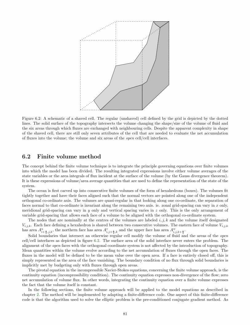
Figure 6.2: A schematic of a shaved cell. The regular (unshaved) cell defined by the grid is depicted by the dottedlines. The solid surface of the topography intersects the volume changing the shape/size of the volume of fluid andthe six areas through which fluxes are exchanged with neighbouring cells. Despite the apparent complexity in shapeof the shaved cell, there are still only seven attributes of the cell that are needed to evaluate the net accumulationof fluxes into the volume; the volume and six areas of the open cell/cell interfaces.

6.2 Finite volume method

The concept behind the finite volume technique is to integrate the principle governing equations over finite volumesinto which the model has been divided. The resulting integrated expressions involve either volume averages of thestate variables or the area integrals of flux incident at the surface of the volume (by the Gauss divergence theorem).It is these expressions of volume/area average quantities that are used to define the representation of the state of thesystem.

The ocean is first carved up into consecutive finite volumes of the form of hexahedrons (boxes). The volumes fittightly together and have their faces aligned such that the normal vectors are pointed along one of the independentorthogonal co-ordinate axis. The volumes are quasi-regular in that looking along one co-ordinate, the separation offaces normal to that co-ordinate is invariant along the remaining two axis. ie. zonal grid-spacing can vary in x only,meridional grid-spacing can vary in y only and vertical spacing varies in z only. This is the only arrangement ofvariable grid-spacing that allows each face of a volume to be aligned with the orthogonal co-ordinate system.

The nodes that are nominally at the centres of the volumes are labeled i, j, k and the volume itself designatedVi,j,k. Each face defining a hexahedron is shared between two consecutive volumes. The eastern face of volume Vi,j,khas area Au

i+ 12,j,k

, the northern face has area Avi,j+ 1

2,k

and the upper face has area Awi,j,k+ 1

2

.

Solid boundaries that intersect an otherwise regular cell modify the volume of fluid and the areas of the open

cell/cell interfaces as depicted in figure 6.2. The surface area of the solid interface never enters the problem. Thealignment of the open faces with the orthogonal coordinate system is not affected by the introduction of topography.Mean quantities within the volume evolve according to the net accumulation of fluxes through the open faces. Thefluxes in the model will be defined to be the mean value over the open area. If a face is entirely closed off, this issimply represented as the area of the face vanishing. The boundary condition of no flux through solid boundaries isimplicitly met by budgeting only with fluxes through open areas.

The pivotal equation in the incompressible Navier-Stokes equations, concerning the finite volume approach, is thecontinuity equation (incompressibility condition). The continuity equation expresses non-divergence of the flow; zeronet accumulation of volume flux. In other words, integrating the continuity equation over a finite volume expressesthe fact that the volume itself is constant.

In the following sections, the finite volume approach will be applied to the model equations as described inchapter 2. The method will be implemented by adapting a finite-difference code. One aspect of this finite-differencecode is that the algorithm used to solve the elliptic problem is the pre-conditioned conjugate gradient method. As

81

implemented, the method is limited to solving positive definite, symmetric matrix problems. This requirement willlimit the form that the finite volume momentum equations can take because the finite volume approach can otherwiselead to an asymmetric matrix problem. We therefore apply the finite volume approach to the continuity and tracerequations but use a less general approach when forming the finite volume momentum equations. The form of themomentum equations will be found that both leads to a symmetric elliptic problem and conserves energy.

6.2.1 Continuity equation and boundary conditions

The continuity equation is the pivotal equation when applying the finite volume approach to the incompressibleNavier-Stokes equations. Integrating continuity over the volume Vi,j,k yields:

∫ ∫ ∫

Vi,j,k

∇ · u dV =

∫ ∫

u · n dA = 0 (6.1)

No normal flow is imposed at solid interfaces, and at the rigid-lid at the surface. This is naturally applied in theintegral divergence form of the continuity equation as written above. The elliptic equation for pressure, that arisesfrom substituting the momentum equations in to the incompressibility condition as written, automatically has theappropriate boundary conditions if use is made of 6.1.

The integrated expression,∫∫

u · n dA, involves only fields evaluated on the surface of the volume. Divergencewithin the interior of the volume is budgeted for implicitly. The area integrals applied to the normal component ofvelocity can be written in terms of the area and mean value of the velocity component. For example, the easternface contribution to the budget is:

∫ ∫

Au

i+ 12

,j,k

u dy dz ≡ Aui+ 12,j,kui+ 1

2,j,k (6.2)

which is simply the definition of the mean value of u on the eastern face multiplied by its area Aui+ 1

2,j,k

.

The integral form of the continuity, for the finite volumes defined above, then takes the form:

Aui+ 1

2,j,k

ui+ 12,j,k − Au

i− 12,j,k

ui− 12,j,k

+ Avi,j+ 1

2,kvi,j+ 1

2,k − Av

i,j+ 12,kvi,j− 1

2,k

+ Awi,j,k+ 1

2

wi,j,k+ 12

− Awi,j,k+ 1

2

wi,j,k− 12

= 0 (6.3)

where the averaging operator has been dropped from the velocities. In short-hand difference notation this is:

δx(Auu) + δx(A

vv) + δz(Aww) = 0 (6.4)

In order to satisfy continuity exactly, the momentum variables in the model are appropriately defined as averagesover respective faces of the volume.

If this is so, then it should be understood that the model variable ui+ 12,j,k, for example, contains no information

about the continuous u field within the volume itself. In the x direction, the representation of the continuum u fieldlooks like a series of delta functions at discrete intervals. Much as in finite differencing, the y-z mean of continuumu matches the model variables at these discrete nodes in the x direction.

Although the foundation of a discretised model have been laid, it should be emphasized that at this stage, insatisfying the integral form of continuity, the discrete model variables are an exact representation of the continuum.There is no truncation error in the evaluation of continuity so long as the model velocities are defined to be themeans over their respective areas.

6.2.2 Tracers

Just as continuity is succinctly handled in the finite volume approach, conservation of tracers is likewise naturallyrepresented. In an incompressible fluid, advection of tracer concentrations (salinity, temperature, etc...) can bewritten as the divergence of advective fluxes (cf. salt conservation):

∂

∂tS + ∇ · (Su) = Q

S(6.5)

82

where QS

represents real sources and sinks (such as molecular diffusion, riverine discharge, chemical reactions, etc...)of the passive tracer S. Integrating over the same finite volume, Vi,j,k, as was used for continuity, gives:

∂

∂t

∫ ∫ ∫

Vi,j,k

S dV +

∫ ∫

uS.n dA =

∫ ∫ ∫

Vi,j,k

QSdV (6.6)

The first term suggests that the volume mean of the tracer is a suitable discrete variable. This has the facilityof unambiguously and directly budgeting for the total amount of tracer in the model, though conservation of highermoments might need further consideration.

The divergence of advective fluxes can be evaluated much as described previously for the continuity equation.Here, however, the flux is the area average of a product of other model variables as opposed to the product of areaaveraged model variables (vS = vS + v′S′). This integral must be expanded and expressed in terms of availablequantities. This will require the parameterization of an eddy flux, as will be shown later.

Evaluation of the source term is dependent upon the particular tracer being considered and will not be dealt within full detail. In general, most sources and sinks can be written as the divergence of a flux, the flux often being aboundary condition on the model associated with the forcing.

Returning to the advection term, the area integral of the flux through the eastern face can be written:∫ ∫

Au

i+ 12

,j,k

uS dy dz = Aui+ 12,j,k ui+ 1

2,j,kS

Au

+

∫ ∫

Au

i+ 12

,j,k

u′S′ dy dz (6.7)

where the primes denote deviations of the continuum field from the mean value on the face.

There are two issues of closure here; one involves expressing SAu

in terms of the volume averaged variable Si,j,kand the other requires parameterization of the eddy flux u′S′yz. The latter has historically been an important issueand many parameterization schemes have been developed to express u′S′yz in terms of the mean quantities. Theseshould be applicable here even though traditionally the eddy flux is averaged over three spatial dimensions and time.

A finite difference approach of minimizing the truncation error in evaluating SAu

could be used which wouldfavour some high order interpolation scheme. However, a property of the continuous system is that it conserveshigher moments under advection. Here, conservation properties are deemed more important than accuracy since theprinciple behind the finite volume approach is one of conservation of volume.

Suppose the advection terms are differenced as:

V∂S

∂t+ δx(A

uuSx) + δy(A

vvSy) + δz(A

wwSz) (6.8)

then conservation of the second moment can be shown as follows.

S(

δxAuuS

x+ δyA

vvSy

+ δzAwwS

z)

= S2 (δxAuu+ δyA

vv + δzAww)

+S(

AuuδxSx

+AvvδySy

+AwwδzSz)

= S2 (δxAuu+ δyA

vv + δzAww)

SxAuuδxS

x

+ SyAvvδyS

y

+ SzAwwδzS

z

−1

4

(

δx(

Auu(δxS)2)

+ δy(

Avv(δyS)2)

+ δz(

Aww(δzS)2))

=S2

2(δxA

uu+ δyAvv + δzA

ww)

+δx

(

Auu1

2o So2x

)

+ δy

(

Avv1

2o So2y

)

+ δz

(

Aww1

2o So2z

)

where oSo2x is the geometric product between neighbouring nodes. The notation is described in section 3.2.The first contribution vanishes since the advecting flow is non-divergent. The second is the discrete analogue of

∇ · 12S

2u and has no net contribution when summed over the model.In difference notation, the full form of the tracer equation is:

∂S

∂t+

1

V

(

δxAu(uS

x+ u′S′) + δyA

v(vSy

+ v′S′) + δzAw(wS

z+ w′S′)

)

= Q (6.9)

83

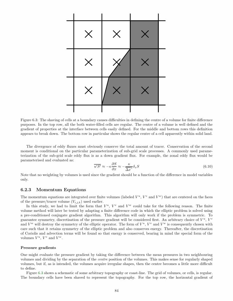
Figure 6.3: The shaving of cells at a boundary causes difficulties in defining the centre of a volume for finite differencepurposes. In the top row, all the both water-filled cells are regular. The centre of a volume is well defined and thegradient of properties at the interface between cells easily defined. For the middle and bottom rows this definitionappears to break down. The bottom row in particular shows the regular centre of a cell apparently within solid land.

The divergence of eddy fluxes must obviously conserve the total amount of tracer. Conservation of the secondmoment is conditional on the particular parameterization of sub-grid scale processes. A commonly used parame-terization of the sub-grid scale eddy flux is as a down gradient flux. For example, the zonal eddy flux would beparameterised and evaluated as:

u′S′ ≈ −κ∂S∂x

≈ − κ

∆xx δxS (6.10)

Note that no weighting by volumes is used since the gradient should be a function of the difference in model variablesonly.

6.2.3 Momentum Equations

The momentum equations are integrated over finite volumes (labeled V u, V v and V w) that are centered on the facesof the pressure/tracer volume (Vi,j,k) used earlier.

In this study, we had to limit the form that V u, V v and V w could take for the following reason. The finitevolume method will later be tested by adapting a finite difference code in which the elliptic problem is solved usinga pre-conditioned conjugate gradient algorithm. This algorithm will only work if the problem is symmetric. Toguarantee symmetry, discretisation of the pressure gradient will be considered first. An arbitrary choice of V u, V v

and V w will destroy the symmetry of the elliptic operator. The form of V u, V v and V w is consequently chosen withcare such that it retains symmetry of the elliptic problem and also conserves energy. Thereafter, the discretisationof Coriolis and advection terms will be found so that energy is conserved, bearing in mind the special form of thevolumes V u, V v and V w.

Pressure gradients

One might evaluate the pressure gradient by taking the difference between the mean pressures in two neighbouringvolumes and dividing by the separation of the centre position of the volumes. This makes sense for regularly shapedvolumes, but if, as is intended, the volumes acquire irregular shapes, then the centre becomes a little more difficultto define.

Figure 6.3 shows a schematic of some arbitrary topography or coast-line. The grid of volumes, or cells, is regular.The boundary cells have been shaved to represent the topography. For the top row, the horizontal gradient of

84

properties between water-filled cells is apparently easily defined by the separation of the centres of the cells. Thecentres are less obviously defined in the middle and bottom rows. The bottom row in particular has the regular cellcentre within land.

In the continuous formulation, a diagnostic elliptic equation for the pressure was found from continuity and themomentum equations. It takes the form:

∇.F = ∇.G − ∂

∂t∇.u (6.11)

where the last term vanishes due to the incompressibility condition. The left hand term becomes the elliptic operator(∇2) on substituting F = ∇p with the right hand side providing the source.

As written, the problem has an infinite set of solutions F that satisfy the lateral boundary conditions since anon-divergent vector field can be added to F . However, the elliptic problem, ∇

2p = ∇ · G, can be equivalentlyexpressed:

∇.F = ∇.G (6.12a)

∇ ∧ F = 0 (6.12b)

This is a well posed problem that has a unique solution [GB79]. The very fact that system 6.12 is equivalent to theelliptic equation for pressure and has a unique solution suggests that the particular representation of F in a discretesense does not change the solution, so long as that discretisation satisfies the zero curl condition.

Since it is F that ensures the non-divergence, rather than the particular discretisation of F , there is someflexibility in its choice of discretisation. Therefore, for the convenience of creating a symmetric elliptic problem, afixed grid spacing is used to evaluate the pressure gradient.

This might seem to ignore the role of the boundaries and boundary conditions in the elliptic problem. However,as was mentioned in the context of the continuity equation, the boundary conditions are applied to the continuityequation in the process of integrating it over finite volumes. Shaving cells modifies the areas and volumes of the cellswhich are explicitly required in the resulting elliptic problem.

The simplest, discrete form of the pressure gradient, that gives rise to a symmetric elliptic problem, is used:

∂u

∂t+

1

ρo

1

∆xx δxp (6.13a)

∂v

∂t+

1

ρo

1

∆yy δyp (6.13b)

∂w

∂t+

1

ρo

1

∆zz δzp (6.13c)

Energy conservation requires an analogue of the property:

u · ∇p = ∇ · (pu) − p∇ · u = ∇ · (pu) (6.14)

which means that the pressure gradient should not contribute to the global energy budget.The discrete form of 6.14 is:

V uu

∆xx δxp

x

+V vv

∆yy δyp

y

+V ww

∆zz δzp

z

=

δx

(

px Vuu

∆xx

)

+

δy

(

py Vvv

∆yy

)

+

δz

(

pz Vww

∆zz

)

−

pδx

(

V uu

∆xx

)

+

pδy

(

V vv

∆yy

)

+

pδz

(

V ww

∆zz

)

(6.15)

where use of 3.12e has been made.The last term should vanish by continuity and this can only happen if:

V u = ∆xxAu (6.16a)

V v = ∆yyAv (6.16b)

V w = ∆zzAw (6.16c)

85

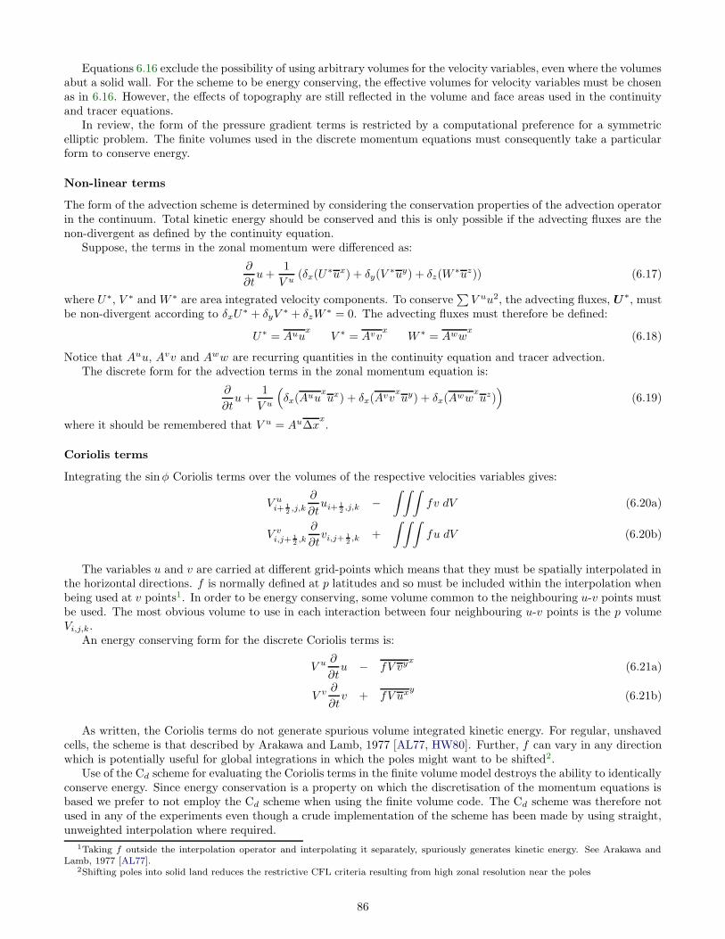
Equations 6.16 exclude the possibility of using arbitrary volumes for the velocity variables, even where the volumesabut a solid wall. For the scheme to be energy conserving, the effective volumes for velocity variables must be chosenas in 6.16. However, the effects of topography are still reflected in the volume and face areas used in the continuityand tracer equations.

In review, the form of the pressure gradient terms is restricted by a computational preference for a symmetricelliptic problem. The finite volumes used in the discrete momentum equations must consequently take a particularform to conserve energy.

Non-linear terms

The form of the advection scheme is determined by considering the conservation properties of the advection operatorin the continuum. Total kinetic energy should be conserved and this is only possible if the advecting fluxes are thenon-divergent as defined by the continuity equation.

Suppose, the terms in the zonal momentum were differenced as:

∂

∂tu+

1

V u(δx(U

∗ux) + δy(V∗uy) + δz(W

∗uz)) (6.17)

where U∗, V ∗ and W ∗ are area integrated velocity components. To conserve∑

V uu2, the advecting fluxes, U ∗, mustbe non-divergent according to δxU

∗ + δyV∗ + δzW

∗ = 0. The advecting fluxes must therefore be defined:

U∗ = Auux

V ∗ = Avvx

W ∗ = Awwx

(6.18)

Notice that Auu, Avv and Aww are recurring quantities in the continuity equation and tracer advection.The discrete form for the advection terms in the zonal momentum equation is:

∂

∂tu+

1

V u

(

δx(Auuxux) + δx(Avv

xuy) + δx(Aww

xuz)

)

(6.19)

where it should be remembered that V u = Au∆xx.

Coriolis terms

Integrating the sinφ Coriolis terms over the volumes of the respective velocities variables gives:

V ui+ 12,j,k

∂

∂tui+ 1

2,j,k −

∫ ∫ ∫

fv dV (6.20a)

V vi,j+ 12,k

∂

∂tvi,j+ 1

2,k +

∫ ∫ ∫

fu dV (6.20b)

The variables u and v are carried at different grid-points which means that they must be spatially interpolated inthe horizontal directions. f is normally defined at p latitudes and so must be included within the interpolation whenbeing used at v points1. In order to be energy conserving, some volume common to the neighbouring u-v points mustbe used. The most obvious volume to use in each interaction between four neighbouring u-v points is the p volumeVi,j,k.

An energy conserving form for the discrete Coriolis terms is:

V u∂

∂tu − fV vy

x(6.21a)

V v∂

∂tv + fV ux

y(6.21b)

As written, the Coriolis terms do not generate spurious volume integrated kinetic energy. For regular, unshavedcells, the scheme is that described by Arakawa and Lamb, 1977 [AL77, HW80]. Further, f can vary in any directionwhich is potentially useful for global integrations in which the poles might want to be shifted2.

Use of the Cd scheme for evaluating the Coriolis terms in the finite volume model destroys the ability to identicallyconserve energy. Since energy conservation is a property on which the discretisation of the momentum equations isbased we prefer to not employ the Cd scheme when using the finite volume code. The Cd scheme was therefore notused in any of the experiments even though a crude implementation of the scheme has been made by using straight,unweighted interpolation where required.

1Taking f outside the interpolation operator and interpolating it separately, spuriously generates kinetic energy. See Arakawa andLamb, 1977 [AL77].

2Shifting poles into solid land reduces the restrictive CFL criteria resulting from high zonal resolution near the poles

86

6.2.4 Numerical stability

The linear numerical stability of each individual term in the model can be analyzed. This does not guarantee overallstability but it is invariably a good guide for choosing the model and numerical parameters.

The quasi-second order Adams-Bashforth scheme (ABII) is used for all terms except the pressure gradient. Theanalysis of this scheme is complicated but it suffices to satisfy a CFL criteria similar to a forward in time discretisationfor non oscillatory terms.

On a regular grid, a time-lagged diffusion term (forward in time, centered in space - FTCS) is differenced as:

1

∆t(φn+1 − φn) =

κ

∆x2(φni−1 − 2φni + φni+1) (6.22)

Substituting in a solution of the form e−λteıkx yields:

e−λ∆t − 1 =κ∆t

∆x2(e−ık∆x − 2 + eık∆x)

=κ∆t

∆x2(2 cos k∆x− 2)

= −4κ∆t

∆x2sin2 k∆x

2

e−λ∆t = 1 − 4κ∆t

∆x2sin2 k∆x

2(6.23)

For the scheme to be stable, the amplification factor e−λ∆ must be less than 1 in absolute magnitude; |e−λ∆| ≤ 1.This leads to the stability criterion:

2κ∆t

∆x2≤ 1 (6.24)

For more than one dimension, each dimension contributes a term on the left hand side of the inequality of the sameform.

Note that for the upper limit (satisfying the equality), the amplification factor is negative. This implies that λis imaginary and so the solution is oscillatory. To ensure that all wave numbers decay without spurious oscillations,one must satisfy the criterion:

4κ∆t

∆x2≤ 1 (6.25)

In principle, at the upper limit of this inequality, a pure grid length wave (k = π/∆x) is instantaneously damped tozero amplitude.

This simple example is presented as an analogue for analyzing the stability of the discretisation described in thischapter. The general form for diffusion in the finite volume model is:

∂

∂tφ =

∆t

Vδx(

κA

∆xδxφ) (6.26)

where V , A, κ and ∆x can all be functions of x. For convenience, define:

γi+ 12

=∆tκi+ 1

2Ai+ 1

2

Vi∆xi+ 12

γi− 12

=∆tκi− 1

2Ai− 1

2

Vi∆xi− 12

so that the amplification equation can be written:

e−λ∆t − 1 = γi+ 12(cos k∆x− ı sin k∆x− 1) − γi− 1

2(− cos k∆x+ ı sin k∆x+ 1)

= (γi+ 12

+ γi− 12)(cos k∆x− 1) + ı(γi+ 1

2− γi− 1

2) sin k∆x

= (γi+ 12

+ γi− 12)(−2 sin2 k∆x

2) + ı(γi+ 1

2− γi− 1

2)2 sin

k∆x

2cos

k∆x

2(6.27)

If γ varies across a grid-cell, the amplification factor has an imaginary component. The stability condition for eachwave number is:

(

1 − 2(γi+ 12

+ γi− 12) sin2 k∆x

2

)2

+ 4(γi+ 12− γi− 1

2)2 sin2 k∆x

2(1 − sin2 k∆x

2) ≤ 1 (6.28)

87

The maximum value of the left hand side is at k = π/∆x if γ is always positive (as it should be). The overall stabilitycriterion is therefore:

2(γi+ 12

+ γi− 12) =

4∆t

V

(

κA

∆x

)x

≤ 1 (6.29)

which must be satisfied at each point in the model. For regular gridding the criteria reduces to 6.24.The Courant number for the advection terms is equivalently:

∆t

VuA

x(6.30)

where Ax/V , in both 6.29 and 6.30, takes the role of a grid length, ∆x.

The stability criterion 6.29 has implications for shaving cells to represent topography. Volumes can not beallowed to become arbitrarily small without adversely requiring a smaller time-step. To be able to shave cells in anunrestricted manner would require an implicit evaluation of most terms in the model. An alternative is to limit theminimum volume of a cell to some fraction of an unshaved cell. This is done by either filling or emptying the cellwith land by some small amount.

6.2.5 Comment on Accuracy

The accuracy of the finite volume method is second order in the interior. This is qualified because the areas andvolumes are regular in the interior and so the scheme is equivalent to a second order, finite different rendition of themodel.

The accuracy of models at solid boundaries is a long disputed issue (see Dukowicz and Dvinsky, 1992 [DD92]).At the boundaries, shaving cells is analogous to changing the grid-size. This means that the differencing is no longercentered so the accuracy must drop to first order for shaved cells at the boundaries.

6.3 Testing the finite volume approach

Two experiments, each of a very different nature, have been chosen to illustrate the potential of this finite volumeapproach for the treatment of topography. The experiments involve well known interactions with topography.

Topographic β effect: Steady, inviscid and linear flow of a homogeneous rotating fluid must, by the Taylor-Proudman theorem, follow contours of f/H . Variations in f/H can be due to a planetary vorticity gradient,β, or to a sloping bottom.

Flow over a Gaussian bump: The interaction of a zonal flow with tall isolated sea-mounts have been modelledextensively. The circulation resulting from stratified flow over a tall Gaussian bump in a periodic channel ismodelled; solutions from the SPEM code (σ co-ordinate) and the finite volume approach are compared.

6.3.1 Topographic β

We configured the model on a β-plane with one homogeneous, flat-bottomed layer and forced by a sinusoidal wind-stress. The resulting flow is the Stommel solution; zonally asymmetric due to the anisotropic propagation of Rossbywaves in the planetary potential vorticity gradient. On an f-plane, shallowing of the basin towards the north createsan equivalent PV gradient. This is modelled by shaving the bottom off the layer as a function of latitude. Theresulting circulation can be made identical to the β-plane solution if the layer depth is appropriately chosen.

If the Rossby number is small, the potential vorticity of a homogeneous layer is f/H , where f is the Coriolisparameter and H is the depth of the fluid.

On a β-plane, the potential vorticity and its meridional gradient are, for a flat bottomed ocean of depth Ho:

Q =fo + βy

Ho;

∂Q

∂y=

β

Ho(6.31)

On an f -plane with variable H , the meridional potential vorticity gradient is:

Q =foH(y)

;∂Q

∂y=

−foH(y)2

∂H

∂y(6.32)

88

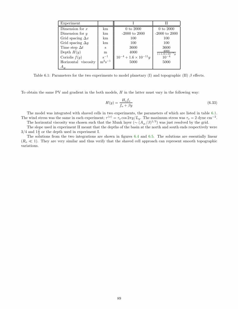
Experiment I II

Dimension for x km 0 to 2000 0 to 2000Dimension for y km -2000 to 2000 -2000 to 2000Grid spacing ∆x km 100 100Grid spacing ∆y km 100 100Time step ∆t s 3600 3600Depth H(y) m 4000 4000

1+1.6×10−7y

Coriolis f(y) s−1 10−4 + 1.6 × 10−11y 10−4

Horizontal viscosityA

H

m2s−1 5000 5000

Table 6.1: Parameters for the two experiments to model planetary (I) and topographic (II) β effects.

To obtain the same PV and gradient in the both models, H in the latter must vary in the following way:

H(y) =Hofofo + βy

(6.33)

The model was integrated with shaved cells in two experiments, the parameters of which are listed in table 6.1.The wind stress was the same in each experiment; τ (x) = τo cos 2πy/Ly. The maximum stress was τo = 2 dyne cm−2.

The horizontal viscosity was chosen such that the Munk layer (∼ (AH/β)1/3) was just resolved by the grid.

The slope used in experiment II meant that the depths of the basin at the north and south ends respectively were3/4 and 1 1

2 or the depth used in experiment I.The solutions from the two integrations are shown in figures 6.4 and 6.5. The solutions are essentially linear

(Ro 1). They are very similar and thus verify that the shaved cell approach can represent smooth topographicvariations.

89

-2000

-1500

-1000

-500

0

500

1000

1500

2000

Y

0 500 1000 1500 2000

X

0.10 m s-1

-0.03

-0.0

3

-0.03

-0.0

3

-0.015

-0.015

-0.0

15

-0.015

-0.015

-0.015

00

0

0

0

0

0

00

0.015

0.015

0.01

5

0.015

0.015

0.015

0.01

5

0.03

0.03

Figure 6.4: Pressure and velocity vectors at t = 1 yr for the flat bottomed β-plane integration.90

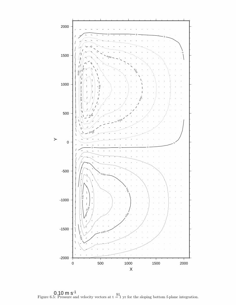
-2000

-1500

-1000

-500

0

500

1000

1500

2000

Y

0 500 1000 1500 2000

X

0.10 m s-1

-0.0

3

-0.03

-0.03

-0.0

3

-0.015

-0.015

-0.0

15

-0.015

-0.015

-0.0

15

0 00

0

0

000

0.015

0.015

0.01

5

0.015

0.015

0.03

0.03

Figure 6.5: Pressure and velocity vectors at t = 1 yr for the sloping bottom f-plane integration.91

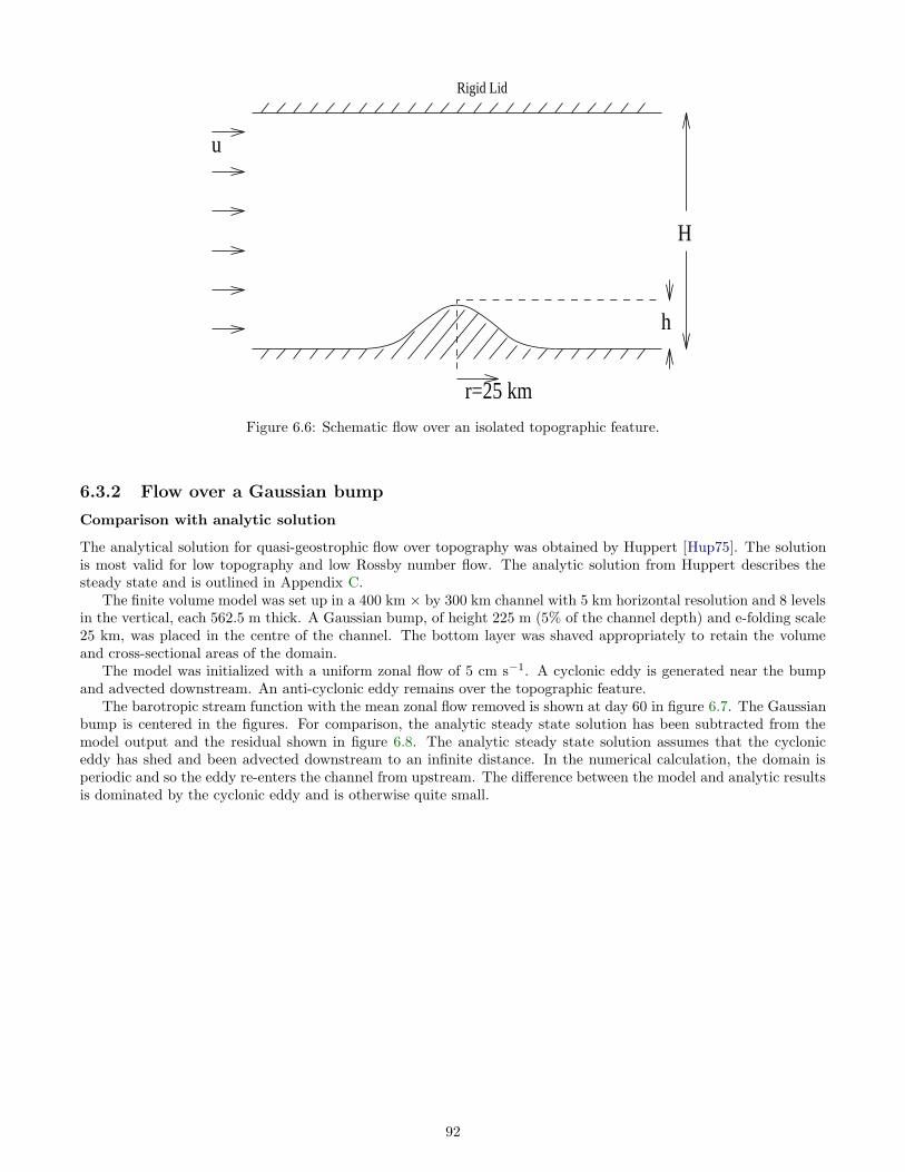
r=25 km

h

H

u

Rigid Lid

Figure 6.6: Schematic flow over an isolated topographic feature.

6.3.2 Flow over a Gaussian bump

Comparison with analytic solution

The analytical solution for quasi-geostrophic flow over topography was obtained by Huppert [Hup75]. The solutionis most valid for low topography and low Rossby number flow. The analytic solution from Huppert describes thesteady state and is outlined in Appendix C.

The finite volume model was set up in a 400 km × by 300 km channel with 5 km horizontal resolution and 8 levelsin the vertical, each 562.5 m thick. A Gaussian bump, of height 225 m (5% of the channel depth) and e-folding scale25 km, was placed in the centre of the channel. The bottom layer was shaved appropriately to retain the volumeand cross-sectional areas of the domain.

The model was initialized with a uniform zonal flow of 5 cm s−1. A cyclonic eddy is generated near the bumpand advected downstream. An anti-cyclonic eddy remains over the topographic feature.

The barotropic stream function with the mean zonal flow removed is shown at day 60 in figure 6.7. The Gaussianbump is centered in the figures. For comparison, the analytic steady state solution has been subtracted from themodel output and the residual shown in figure 6.8. The analytic steady state solution assumes that the cycloniceddy has shed and been advected downstream to an infinite distance. In the numerical calculation, the domain isperiodic and so the eddy re-enters the channel from upstream. The difference between the model and analytic resultsis dominated by the cyclonic eddy and is otherwise quite small.

92

0 50 100 150 200 250 300 350 4000

50

100

150

200

250

300

−7−6

−5

−5

−4

−4

−3

−3

−3

−2

−2

−2

−2

−1

−1

−1

−1

00

0

0

0

0

11

1

1

11

1

1

222

2

2

2

3

3

4

Figure 6.7: Barotropic stream function at day 60 with constant zonal flow removed.

0 50 100 150 200 250 300 350 4000

50

100

150

200

250

300

0

0

0

0

11

1

1

1

1

1

1

22

2

2

2

2

3

3

3

4

5

Figure 6.8: Barotropic stream function at day 60 with analytic solution removed.

93

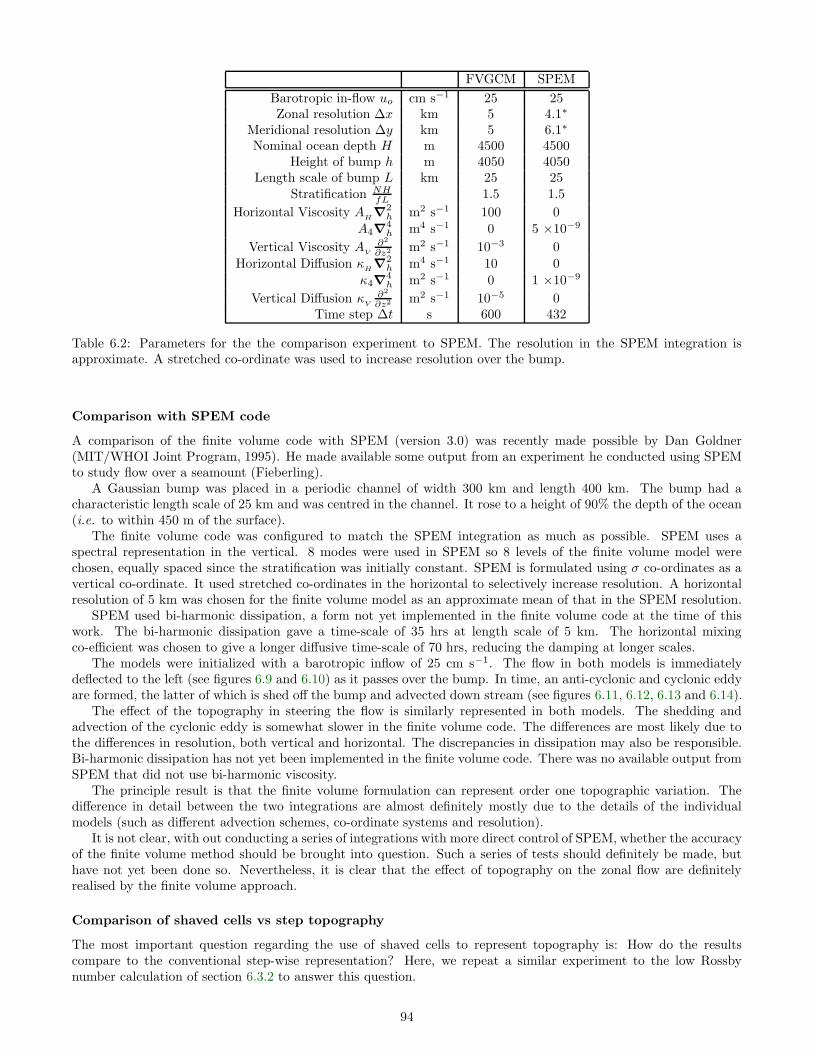
FVGCM SPEM

Barotropic in-flow uo cm s−1 25 25Zonal resolution ∆x km 5 4.1∗

Meridional resolution ∆y km 5 6.1∗

Nominal ocean depth H m 4500 4500Height of bump h m 4050 4050

Length scale of bump L km 25 25Stratification NH

fL 1.5 1.5

Horizontal Viscosity AH

∇2h m2 s−1 100 0

A4∇4h m4 s−1 0 5 ×10−9

Vertical Viscosity AV

∂2

∂z2 m2 s−1 10−3 0

Horizontal Diffusion κH

∇2h m4 s−1 10 0

κ4∇4h m2 s−1 0 1 ×10−9

Vertical Diffusion κV

∂2

∂z2 m2 s−1 10−5 0Time step ∆t s 600 432

Table 6.2: Parameters for the the comparison experiment to SPEM. The resolution in the SPEM integration isapproximate. A stretched co-ordinate was used to increase resolution over the bump.

Comparison with SPEM code

A comparison of the finite volume code with SPEM (version 3.0) was recently made possible by Dan Goldner(MIT/WHOI Joint Program, 1995). He made available some output from an experiment he conducted using SPEMto study flow over a seamount (Fieberling).

A Gaussian bump was placed in a periodic channel of width 300 km and length 400 km. The bump had acharacteristic length scale of 25 km and was centred in the channel. It rose to a height of 90% the depth of the ocean(i.e. to within 450 m of the surface).

The finite volume code was configured to match the SPEM integration as much as possible. SPEM uses aspectral representation in the vertical. 8 modes were used in SPEM so 8 levels of the finite volume model werechosen, equally spaced since the stratification was initially constant. SPEM is formulated using σ co-ordinates as avertical co-ordinate. It used stretched co-ordinates in the horizontal to selectively increase resolution. A horizontalresolution of 5 km was chosen for the finite volume model as an approximate mean of that in the SPEM resolution.

SPEM used bi-harmonic dissipation, a form not yet implemented in the finite volume code at the time of thiswork. The bi-harmonic dissipation gave a time-scale of 35 hrs at length scale of 5 km. The horizontal mixingco-efficient was chosen to give a longer diffusive time-scale of 70 hrs, reducing the damping at longer scales.

The models were initialized with a barotropic inflow of 25 cm s−1. The flow in both models is immediatelydeflected to the left (see figures 6.9 and 6.10) as it passes over the bump. In time, an anti-cyclonic and cyclonic eddyare formed, the latter of which is shed off the bump and advected down stream (see figures 6.11, 6.12, 6.13 and 6.14).

The effect of the topography in steering the flow is similarly represented in both models. The shedding andadvection of the cyclonic eddy is somewhat slower in the finite volume code. The differences are most likely due tothe differences in resolution, both vertical and horizontal. The discrepancies in dissipation may also be responsible.Bi-harmonic dissipation has not yet been implemented in the finite volume code. There was no available output fromSPEM that did not use bi-harmonic viscosity.

The principle result is that the finite volume formulation can represent order one topographic variation. Thedifference in detail between the two integrations are almost definitely mostly due to the details of the individualmodels (such as different advection schemes, co-ordinate systems and resolution).

It is not clear, with out conducting a series of integrations with more direct control of SPEM, whether the accuracyof the finite volume method should be brought into question. Such a series of tests should definitely be made, buthave not yet been done so. Nevertheless, it is clear that the effect of topography on the zonal flow are definitelyrealised by the finite volume approach.

Comparison of shaved cells vs step topography

The most important question regarding the use of shaved cells to represent topography is: How do the resultscompare to the conventional step-wise representation? Here, we repeat a similar experiment to the low Rossbynumber calculation of section 6.3.2 to answer this question.

94

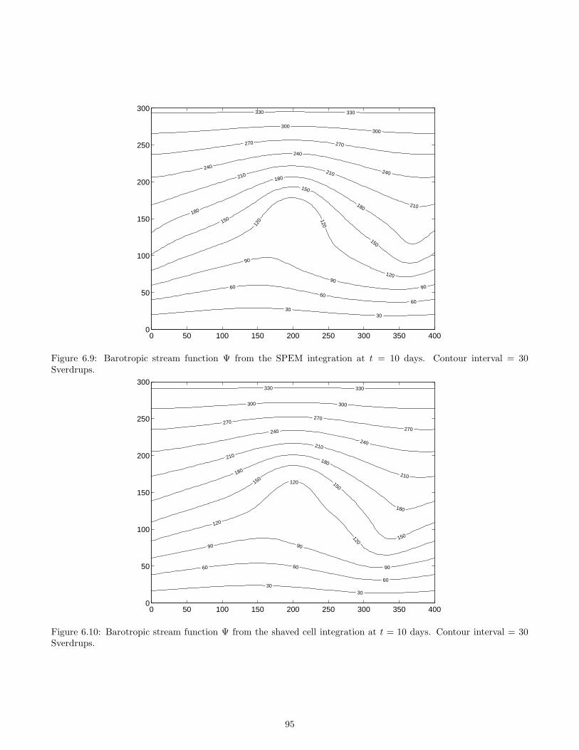
0 50 100 150 200 250 300 350 4000

50

100

150

200

250

300

3030

60

6060

90

9090

120 120

120

150

150

150

180

180

180

210210

210

240

240

240

270 270

300300

330 330

Figure 6.9: Barotropic stream function Ψ from the SPEM integration at t = 10 days. Contour interval = 30Sverdrups.

0 50 100 150 200 250 300 350 4000

50

100

150

200

250

300

3030

60 60

60

90 90

90

120

120

120

150150

150

180

180

180

210

210

210

240

240

270270

270

300 300

330 330

Figure 6.10: Barotropic stream function Ψ from the shaved cell integration at t = 10 days. Contour interval = 30Sverdrups.

95

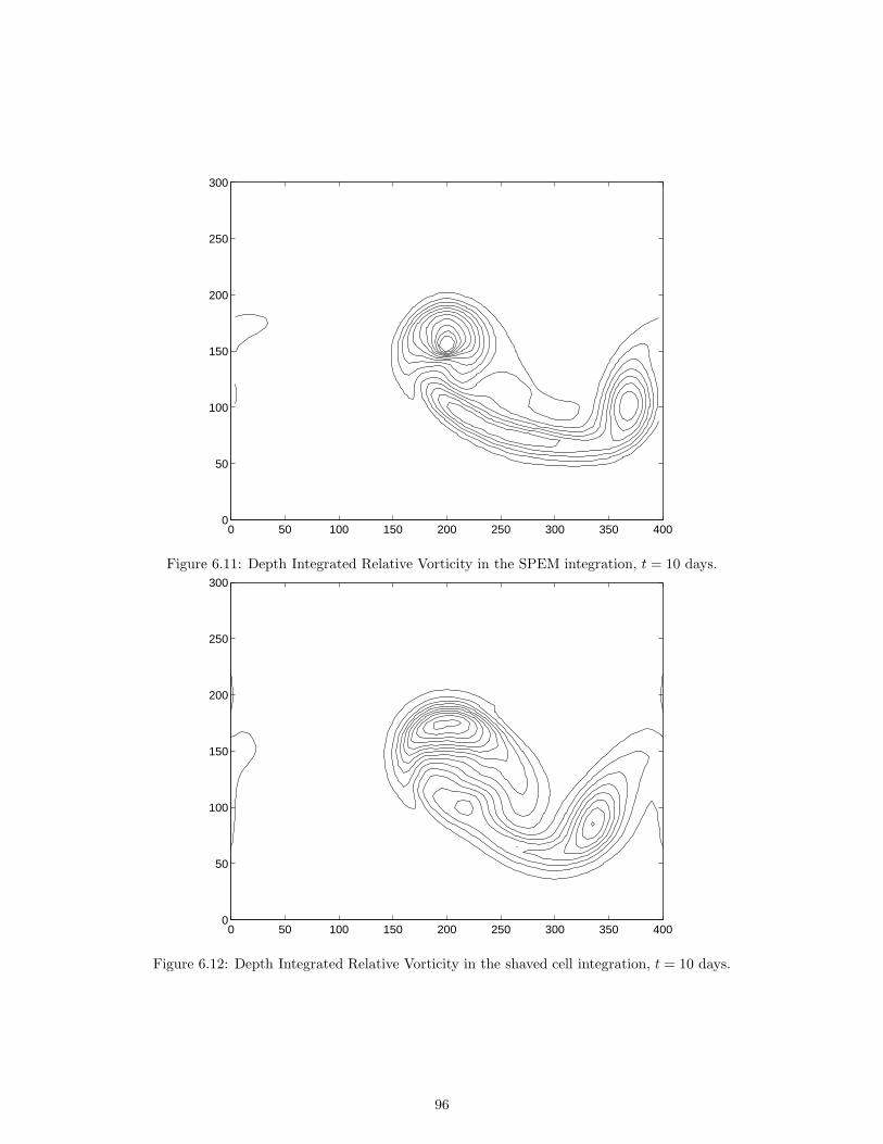
0 50 100 150 200 250 300 350 4000

50

100

150

200

250

300

Figure 6.11: Depth Integrated Relative Vorticity in the SPEM integration, t = 10 days.

0 50 100 150 200 250 300 350 4000

50

100

150

200

250

300

Figure 6.12: Depth Integrated Relative Vorticity in the shaved cell integration, t = 10 days.

96

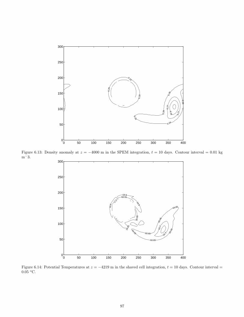
0 50 100 150 200 250 300 350 4000

50

100

150

200

250

300

0.26

0.27

0.27

0.28

0.28

0.28

0.28

0.28

0.29

0.29

0.29

Figure 6.13: Density anomaly at z = −4000 m in the SPEM integration, t = 10 days. Contour interval = 0.01 kgm−3.

0 50 100 150 200 250 300 350 4000

50

100

150

200

250

300

18.55

18.6

18.6

18.6

18.6

5

18.6

5

18.6

5

18.65

18.65 18.65

18.6

5

18.65

18.7

18.7

Figure 6.14: Potential Temperatures at z = −4219 m in the shaved cell integration, t = 10 days. Contour interval =0.05 oC.

97

−4500

−3937.5

−3375

200130 270

L8

L7

Figure 6.15: Schematic of the bottom two layers in the eight layer integrations using first “step-topography” andthen “shaved-cells” to represent a Gaussian bump. The regular model cells are indicated by the dotted grid. Thecontinuous curve is the Gaussian topography to be modelled. The large pill-box curve is the “best” representationof the Gaussian that can be managed using step-wise topography. Since the graphical presentation of areas andvolumes is awkward, the curve used to calculate the volumes and areas is presented. The curve is described on agrid of three times higher resolution than that of the model. It should be apparent to the eye that the volumes andareas used in the finite volume calculation are consequently for more representative of the “true” volumes and areasthan in the step-wise calculation.

98

The Gaussian bump now has a height of 15% of the fluid depth. Figure 6.15 shows the analytic, step-wiseand finite-volume representations of the Gaussian function. The model cells are depicted by the dashed grid. Thehorizontal resolution of 5 km amply resolves the 25 km exponential scale of the Gaussian function. The analyticfunction penetrates the second deepest layer of the model. The step-wise representation of the Gaussian bump isas a pill-box, of crudely the same volume, that fills cells in the bottom layer of the model. The stair-case curve isthe numerical approximation to the analytic function used for calculating the volumes and areas used in the finitevolume method.

The volumes and areas are calculated as follows. The analytic function is evaluated on a fine grid of threetimes higher resolution and these values are used as the height of pill-boxes. The volumes of the pill-boxes are thensummed up over each model cell and the result is used for the volume of the model cell. The face area of model cellsis calculated by summing up the face areas of the fine-grid pill-boxes abutting a model face. As the resolution of thefine-grid is increased, the method asymptotes to an analytic method of evaluating the volumes and areas.

The models were initialised and integrated as before. Figures 6.16 and 6.17 show the potential temperature at adepth of 3656 m (corresponding to the second deepest layer) at the end of 1 day. In the shaved cell integration (6.17),the anti-cyclonic eddy is moving clockwise around the bump whilst the cyclonic eddy is beginning to be influencedby the mean zonal flow. The step-wise integration is significantly different. The anti-cyclonic eddy has not beencarried clockwise around the bump, possibly because of the angularity of the feature. The strength of the eddies isapproximately the same, though they are closer in separation, presumably because the feature is narrower. In short,the solution for the step-wise representation of the Gaussian bump bears minimal resemblance to the solutions ofthe previous sections. Indeed, the solution must presumably look more like that for flow over a cylinder, since thatis what the topography of the model looks like.

In this example, the horizontal scale of topographic variation was resolved. To resolve the Gaussian bumpaccurately in the vertical, the conventional step-wise method would require about 30 layers in place of the bottom1.5 layers. The finite volume method allows the model to realise the slowly varying height of the bump even thoughmost of the variation occurs within just one equivalent model layer.

99

0 50 100 150 200 250 300 350 4000

50

100

150

200

250

300

X (km)

Y (

km) 18.8

18.81

18.81 18.81

18.82

18.8

2

18.8218.82

18.82

18.8318.83

18.83

18.8

3

18.83 18.8318.83

18.8418.84

18.84 18.84 18.84

18.85

18.85

Figure 6.16: Potential temperature at z=-3656 m and t=1 day using the step-wise representation of topography.

0 50 100 150 200 250 300 350 4000

50

100

150

200

250

300

X (km)

Y (

km) 18.8

18.8

1

18.81

18.8118.81

18.82

18.82

18.82

18.8

2

18.8218.82

18.8

3

18.8318.83

18.8318.83

18.83

18.8

3

18.83

18.84

18.84

18.8418.84

18.84

18.8518.85

18.85

18.85

18.86

18.86

Figure 6.17: Potential temperature at z=-3656 m and t=1 day using the shaved cell representation of topography.

100

6.4 Conclusions

A finite volume approach to modelling the ocean has been outlined. The final form of the scheme was dictated byconsiderations of energy conservation. The opportunity for implementing such a technique arose because the originalmodel was formulated on a C grid.

The motivation for developing the finite volume model was to improve the representation of topography. Inparticular, topography controls the circulation by modulating the passages through which basins communicate.Wave interaction with finite slopes also influences the circulation.

Two experiments illustrated the effects of topography and the potential of the scheme to model them better.The topographic β effect was succinctly illustrated. Taylor cap formation was modelled and the results comparedto an almost equivalent SPEM integration. The details of the simulations differed and it is supposed, though notdemonstrated, that these differences led to the different shedding time of the cyclonic eddy.

A third set of experiments compared the shaved-cell method with the conventional step-wise representation oftopography. The results clearly indicate that the finite volume approach is an improvement over step-wise topography.

The accuracy of the scheme is left in question, a conclusion drawn from the comparison with SPEM code.Nevertheless, the reproduction of analytic solutions and the clear improvement over step-wise topography suggestthat the shaved cell method could substantially improve the representation of topographic effects in existing heightcoordinate models.

101

Chapter 7

Concluding remarks

Of the ocean models in existence, most can be grouped into one of two categories; large scale circulation models andsmall scale process study models.

Large scale circulation models are designed for studying the slow large scale circulation patterns of gyres and themeridional overturning. They are typically used:

• to study the role of wind and thermal forcing in determining these large scale patterns.

• to study interactions with the atmosphere.

• to understand the role of the ocean in the climate system.

• in a diagnostic role with observations to estimate the present state of the ocean circulation.

Process study models, on the other hand, are used to study the dynamical behaviour of the oceans on regional andsmaller scales which often involve resolving relatively fast processes (such as gravity waves). These include studiesof the convective overturning process, the nature of dynamical instabilities, the formation of boundary layers andsubsequent interaction with the atmospheric boundary layer, coastal dynamics and forecasting on a regional basis.

Large scale models and process study models differ in horizontal resolution and often also differ in physics. Thelarge scale studies are inevitably carried out at low resolution; the Rossby radius of deformation is typically 20-60 kmwhilst affordable horizontal resolutions tend to be around 50 km upwards. Process studies are normally carried outat resolutions that at least resolve the geostrophic eddy scale and, if necessary, resolve the convective plume scale,depending on the process being studied.

None of the existing numerical models are well suited to work at both ends of the spectrum. The particularphysics and numerical formulation are decided by the scale at which the model will be applied. A large scale modelis not well suited for use at the small scale and vice versa. This means that the models are also potentially ill-suitedfor use in the middle ground, i.e. at the resolutions that are comparable to the scale of transition for validity ofthe physical approximations. In particular, the validity of the primitive equations at the mesoscale and smaller isquestionable.

There are two main reasons for this “spectral gap” in numerical models:

• The smaller scale physics is computationally more expensive to resolve. The non-hydrostatic physics requiresthe inversion of a three-dimensional elliptic operator whilst hydrostatic physics inverts a two dimensionalproblem. For this reason, a non-hydrostatic model has not been used to study the large scale circulation.

• The different extremes in horizontal resolution dictate that different grids be used for large and small scalemodels. As was explained in chapter 4, coarse resolution models tend to be built on an Arakawa ‘B’ gridand high resolution models (and non-hydrostatic models) are normally built on an Arakawa ‘C’ grid. Theapplication of a ‘C’ grid model at low resolution, or a ‘B’ grid model at very high resolution are prone togrid-scale problems that normally inhibit the forward integration of the models.

Part of the motivation behind building a new ocean circulation model was to build one applicable to both endsof spectrum of spatial scales, and thus build one applicable in the middle ground. Such a model then allows us toevaluate when certain physical approximations become invalid. By no means do we expect the global circulation tobe substantially affected by non-hydrostatic effects, but regional calculations, for example at the Equator, will quitepossibly be dependant on the inclusion of quasi- or non-hydrostatic physics. The advantage of such a versatile model

102

is that the transition between small, regional and global scale calculations is not complicated by the use of differentcodes.

The non-hydrostatic model, described in chapter 3, can be integrated forward at low resolution on a global scale.This is only affordable because of the nature of the pre-conditioner used in the conjugate gradient algorithm. Thoughthe results are not shown here, the non-hydrostatic physics is found to have an insignificant effect on the large scalecirculation. This is as expected from conventional understanding and scaling analyses. The question still remains,at what scale does non-hydrostatic physics begin to play a role? This is not just concerned with the role of verticalinertial effects in the ocean but also with the role of the horizontal Coriolis terms at low latitudes.

7.1 The Cd scheme

An example of the problems arising from using the Arakawa ‘C’ grid at low resolution was given at the end of chapter3. The nature of the problem is connected with the spatial averaging of the Coriolis term on a ‘C’ grid. This is awell documented phenomena and is described and explained in chapter 4.

A new scheme is described and tested in chapter 5 that alleviates this problem. The Cd scheme allows the ‘C’grid model to be integrated forward without any spurious noise problems. It has little computational overhead andinvolves only the introduction of two new horizontal velocity variables, carried on a ‘D’ grid, which are step forwardin parallel to the C grid model. These new variables are used in the evaluation of the Coriolis term for the C grid.We view the scheme as a tool used to improve the representation of the Coriolis term without directly modifying therest of the model.

The model code is consequently now applicable at both high and low resolutions. The Cd scheme is, however,switched off at high resolutions since it is not needed. As it stands, the model has only gone part way towards thegoal of applicability at high and low resolutions since the use of the Cd scheme at low resolutions means that it isnot quite the same model as used at high resolution.

7.2 Shaved cells

Strictly speaking, the opportunity to explore the use of shaved cells to represent topography is a result of the modelbeing formulated on an Arakawa ‘C’ grid. The finite volume approach naturally results in a ‘C’ grid arrangement ofmodel variables.

Conventional height co-ordinate models represent topography by fitting the bathymetry to the discrete depths ofthe model layers, resulting in “step-wise” topography. As an alternative, the finite volume approach allows modelcells to be shaved to fit the topography.

The model is re-formulated in chapter 6 using the finite volume approach. In practice, the resulting algebraicequations on a regular grid are essentially the same as for the finite difference model described in chapter 3. Theresulting discretisation of the finite volume model depends on a restriction imposed on the nature of the ellipticproblem.

A pre-conditioned conjugate gradient algorithm is used to solve the elliptic problem. The algorithm is applicablebecause the matrix is symmetric. It was desired that this property be retained for the purposes of efficiency. Thismeant that the finite volume approach could not be applied in a completely general manner to the momentumequations. Nevertheless, the effects of topography are captured in the discrete form of the continuity and tracerequations. The criteria for the discretisation of the momentum equations is based primarily on consideration ofenergy conservation.

Two distinct examples of oceanographic interest are used to demonstrate the potential of using shaved cellsto represent topography. The topographic β effect is modelled and the solution compared to a Stommel solutionobtained on a β-plane. The solutions are indistinguishable.

The interaction of flow with an isolated topographic feature is modelled by placing a Gaussian bump in a channelwith a barotropic zonal flow. A low Rossby number solution is compared to an analytic solution and shown tobe favourably accurate. Comparison of a high Rossby number solution with one obtained using the SPEM codedemonstrates that the shaved cell representation allows the model to realise the effects of extreme topography. Twoequivalent integrations, one using a step-wise representation of the topographic feature, the other using the shavedcell method, are compared. The shaved cell method clearly represents the topography more accurately than theconventional step-wise method.

The method is thus shown to be able to resolve both shallow and deep changes in topography, even with a smallnumber of levels in the vertical. The same will apply in the horizontal, meaning that coastlines can be representedusing the same shaved cell method. One consequence for global ocean modelling is that despite the usually course

103

horizontal resolution, certain features in the coast-lines may still be realised by the circulation. For example, coastlinesare conventionally represented by meridional or zonal barriers whilst the shaved cell method will allow a coast tobe diagonal across meridians. Just as the height of topography is conventionally made to fit the model depths, thepositions of coasts are moved to fit the model grid. This implies that passages are either widened or narrowed. Theshaved cell method does not have this problem. Indeed, the shaved cell method allows a passage to be narrower thanthe grid-size. Clearly, the dynamic processes involved in flow through passages, such as hydraulic control, are notresolved but the ability to transport properties through the passage is retained. Whether the transports are accurateis not clear at this point.

7.3 Future development of model

The model is currently being used for a wide range of applications, from studies in convection, though studies ofmixed layer dynamics, up to regional simulations and global simulations. Much of this work is possible because ofthe parallel implementation of the model. The parallel design of the non-hydrostatic model is satisfactorily optimal.The two-dimensional solver does not take advantage of the parallel architecture due to the choice of mapping to theprocessors.

A move to a free surface formulation is planned that we anticipate will improve the performance of the two-dimensional solver. Dukowicz and Smith, 1995 [DS94], point out that elimination of the rigid-lid approximation hasseveral advantages; among others it computes the surface height directly, allowing comparison with and assimilationof altimetry data and it improves the accuracy of the representation of long Rossby waves.

This issue is raised here because this model has a significant advantage over some others in the use of a freesurface. The free surface formulation re-introduces the external inertia-gravity mode which is filtered out by therigid-lid approximation. The external mode has a phase and group speed of

√gH, as shown in section 2.3.1. The

important point is that the deformation radius,√

gH/f2, is of the order of 1000 km. This means that the waveresolution is inevitably very high. In this limit, a ‘B’ grid model is severely prone to a checker board mode in thepressure field. In contrast, the ‘C’ grid model is very well suited for resolving the external gravity wave motion anddoes so accurately.

7.4 Future directions in ocean modelling

Historically, the low resolution restrictions imposed by the computer technology has lead to an emphasis in thedevelopment of sub-grid scale parameterizations. Even with the recent improvements in computer architectures,there is still a need for better parameterizations of all sub-grid scale processes. This will always be the case untilcomputer technology advances far enough to allow large scale models to resolve the three dimensional turbulencescales.

The need for future model development should also not be underestimated. The need for more versatile modelshas been outlined. The general circulation model described here has been designed to be applicable at many scales.However, there is a further degree of versatility that has yet to be made accessible which is the ability to model awide range of time-scales.

Much current and future climate research explores the natural variability and the predictability of the climatesystem on time-scales from seasons upwards to centuries. There is much interest in devising methods to find andcharacterize steady states of the thermohaline circulation, and the stability of these states to perturbations. Theabove all involve extended prognostic integrations over periods long relative to the dynamical time scales of theindividual sub-systems.

In ocean models based upon the primitive equations, there remains a practical restriction on the time step requiredfor making long integrations. The restriction is due to the natural frequencies of the physics explicitly carried inthe model. One avenue of investigation has been to further approximate the physics, filtering out intermediate timescale processes (eg. gravity waves) by careful scaling of the equations of motion. This has led to the developmentof a whole class of intermediate models (eg. Balance Equations, Semi-geostrophic models, etc) that have proveduseful and certainly will be for some time to come. However, these intermediate models can be difficult to solveand are often limited in their application to other than idealized studies. One example of a particularly successfulintermediate model is the Planetary Geostrophic Equations (see Maier-Reimer et al., 1993 [MRMH93]). This modelhas been integrated for thousands of years in various studies of variability of the thermohaline circulation. However,the model does have approximated physics and thus excludes the possibility of some processes.

An alternative to changing the continuous equations, is to integrate the unapproximated equations implicitly.This technique has advantages since if the resolution is such that an otherwise implicit process is resolved, then it

104

will be accurately represented. Implicit evaluation of physics often leads, however, to a more complicated numericalalgorithm, but interestingly one which often resembles the filtered models.

Implicit techniques are already frequently used to represent physics in ocean modeling. The simplest, commonexample is the implicit evaluation of the Coriolis term in the models based on the Arakawa B grid, such as the GFDLMOM code. This allows a time step longer than the half period of an inertial oscillation and in this case, the inertialoscillation is damped.

Another example is that of filtering the external gravity wave. Here, an explicit free surface would typicallyrequire a time-step of around 10 minutes. The rigid lid approximation filters this mode and makes the effective wavespeed infinite and produces an elliptic equation to be solved for the surface pressure at each longer time-step of themodel. If the free surface is treated implicitly then an elliptic problem again arises but slows the waves down towhatever the resolution can sustain. For very long time steps, the rigid lid and implicit free surface models actuallyconverge in their formulation which is consistent with, and in some ways is a validation of, the approximation atlonger time scales.

There is, in fact, a great deal of similarity, from an algorithmic point of view, between filtered models and implicitmodels based upon the HPEs. There is, as a result, some comparison in computational efficiency between the twoclasses of model. Combined with the simple practical need to integrate the HPEs with long time steps, a return toimplicit methods is possible and certainly worth pursuing.

A certain proportion of the numerical knowledge needed to make models fully implicit already exists. Oceanmodellers have been taking advantage of some of these methods but as of yet, no physically complete model has beenwritten on an implicit basis. Atmospheric GCMs generally incorporate the gravity waves implicitly. The approachused there would obviously be a sound starting point. Development of numerical methods concentrating on shiftingocean models onto an implicit footing would be a significant improvement on our current ability to study the longtime scales mentioned before.

The objective of making ocean models fully or semi-implicit has several immediate applications:i) Ocean models with very long time steps essentially become steady state solvers. The steady state is interesting

in its own right but is inevitably also a common starting point for many other studies such as sensitivity studies.ii) Because the complete physics is still incorporated within the model, the same model used to find the initializing

steady state can be used in process studies, dependent upon the fast physics.iii) The importance of the fast physics in climate variability and stability can be ascertained by using the same

model in its various degrees of implicitness.As already mentioned, implicit physics often leads to a more complicated algebraic formulations of the model.

The solution techniques currently employed already outperform the equivalent explicit models. Indeed, the increasein computational efficiency gained by use of modern techniques (multi-grid, pre-conditioned conjugate gradient) isin fact comparable to that gained by recent innovations in computer hardware. Nevertheless, development andapplication of these techniques in ocean modeling is only in its infancy and as of yet has only recently begun to takeadvantage of the new parallel computer technologies.

The work of this thesis represents only a small step towards the goal of developing a fully versatile model. Theapplicability of the model to many spatial scales is only a beginning. With no changes to the kernel necessary, thecode accommodates both periodic domains, curvi-linear coordinate systems, hydrostatic, quasi- and non-hydrostaticphysics. Perhaps the most beneficial innovation is the use of the finite volume formulation that not only allows veryeasy inclusion of any arbitrary topography but further naturally handles the boundary conditions. The final code isone that can be applied in a wide range of oceanic studies.

105

Appendix A

Derivation of the Navier-StokesEquations of Oceanic Motion

Here, the Navier-Stokes equations that govern fluid flow will be derived in an inviscid context. The accompanyingthermodynamics will also be described to yield the fundamental equations that describe oceanic motions on a rotatingplanet. The derivation is concise but accurate.

Excepting for the discussion on thermodynamics, the derivation is made in an Eulerian frame rather than theconventional Lagrangian frame. The Eulerian frame is concerned with the rates of changes of quantities per unitvolume, which is a convenient property when formulating discrete, numerical models. The Lagrangian frame is moreconventional because the total derivative is the rate of change following a particle. It deals with with the change inconcentration of quantities, or mass of quantity per unit mass of fluid. The Navier-Stokes equations are summarisedin section 2.1.

A.1 Conservation of Mass

A fundamental principle in fluid mechanics is the conservation of mass. For a fluid of density ρ (density is mass perunit volume), the rate of change of mass in a small volume, ∂

∂t

∫∫∫

ρdV , must equal the accumulation of mass fluxinto the volume,

∫∫

ρu.n dS. In the limit of infinitesimal volume, the statement of conservation of mass becomes:

∂

∂tρ+ ∇ · (ρu) = 0 (A.1)

The mass flux, ρu, that appears in the Eulerian form, is in fact the momentum density (momentum per unitvolume). This quantity will explicitly appear in the momentum equations and scalar conservation equations.

Although mass conservation is the most basic equation governing fluid flow, it is rarely used in the form of A.1to model the ocean due to ill-conditioning of the system. The cause of this lies partly in the fact that typical densityvariations are small compared to the mean value. Further, density variations due solely to the compressibility of thefluid are even smaller. This means that the flow is approximately non-divergent and this condition will later replacethe continuity equation.

Conservation of mass can be written:

∂

∂tρ+ ∇ · (ρu) =

Dρ

Dt+ ρ∇ · u = 0 (A.2)

where DDt is the Lagrangian or total derivative; the rate of change following the motion. For a non-divergent fluid,

∇ · u = 0, the density is conserved in the Lagrangian sense.The non-divergence condition itself, ∇ · u = 0, is referred to as the continuity equation, the reason being that

non-divergence is a statement of continuity of volume. These issues will all be discussed later. In the mean time,equation A.1 will be retained.

A useful relationship that might aid the reader for the rest of this derivation, transforms the Lagrangian or totalderivative to a true flux form Eulerian derivative by making use of the continuity equation. For any scalar field, φ:

ρDφ

Dt= ρ(

∂φ

∂t+ u · ∇φ) =

∂(ρφ)

∂t+ ∇ · (ρφu) (A.3)

106

The total derivative is the rate of change following the parcel of fluid whilst the last form expresses the rate of changefor a fixed volume.

A distinct advantage of the flux form is that is can be immediately integrated over the volume of the fluid toprovide a statement of global conservation. For instance, in the absence of net internal sources and sinks, the totalamount of some property is governed by:

∂

∂t

∫ ∫ ∫

V

ρφ dV =

∫ ∫

S

ρφu.n dS (A.4)

where φ can be any internally conserved scalar concentration or unity. The special case of φ = 1 indicates that thetotal mass of the fluid can be changed only by an influx of matter through the interface enclosing the volume. Forthe ocean, solid boundaries permit no normal mass flux whilst precipitation and evaporation act to add or detractwater from the system.

A.2 Conservation of momentum

Newton’s laws of motion state that linear momentum is conserved. For a fluid of density ρ, the relevant quantityis momentum density ρu or momentum (Newton seconds, N s) per unit volume (m3). For an infinitesimal volumedV = dx dy dz, the total rate of change of a component of momentum is the sum of the local rate of change (withinthe volume) and the convergence of momentum fluxes (arising from differing rates of advection into the volume). Itwill equal the net force acting in each direction:

∂

∂tρu + ∇ · (ρuu) =

∑

i

fi (A.5)

The forces acting on a fluid parcel are the pressure gradient force, the force due the gravitation of the earth andthe Coriolis and centripetal forces (resulting from being in a rotating frame of reference).

The first of these is an internal force. Pressure (force per unit area) acts on all parts of the fluid pushing equallyin each direction. Variations in pressure accelerate the fluid. The force acting on a volume dV = dx dy dz is thechange in pressure ∂p

∂x dx acting across the volume through the area dA = dy dz. The force per unit volume is thus∂p∂x or:

fp = −∇p (A.6)

The gravitational potential is a function of position only and the force acting on a unit volume is given by ρgwhere g = ∇(GMe/r). Here, G is the gravitational constant, Me is the gravitating mass of the earth and r is thedistance from the centre of the earth.

The Coriolis force is a fictitious force but is very important in shaping the dynamics of the ocean. Linearmomentum conservation applies in an inertial frame of reference. The rate of change of some quantity, A, observedin the inertial frame expressed in terms of the rate measured in the rotating frame is given by the relation:

D

DtA

i=

D

DtA

r+ Ω ∧ A

r(A.7)

where the the subscripts i and r indicate the inertial and rotating frames. The ∧ is the vector cross product. Ω isthe rotation vector of the earth.

The velocity in the inertial frame is the velocity in the rotating frame of reference with a part due to the rotationof the co-ordinate system:

ui= u

r+ Ω ∧ x (A.8)

Using this relationship and noting that the total derivative of the position vector is the velocity in the inertialframe, u

i= D

Dtx, gives:D

Dtu

i=

D

Dtu

r+ 2Ω ∧ u

r+ Ω ∧ Ω ∧ x (A.9)

The middle term is the Coriolis acceleration and the last term is the centripetal acceleration. The later is only afunction of position and the equivalent force can be written as the gradient of a potential and is usually combinedwith the gravitational potential to yield and effective potential or gravity, so that:

f c = −2Ω ∧ u (A.10)

107

fg = −ρ∇Φ ; Φ = −GMe

r− Ω2r2

2cos2 φ (A.11)

The unapproximated form for the momentum equations is then:

∂

∂tρu + ∇ · (ρuu) + 2Ω ∧ ρu + ρ∇Φ + ∇p = 0 (A.12)

which can be written in Lagrangian form as:

ρ

(

Du

Dt+ 2Ω ∧ u + ∇Φ

)

+ ∇p = 0 (A.13)

The kinetic energy density (kinetic energy per unit volume) is K = 12ρu · u. The kinetic energy equation can be

obtained by taking the scalar product of velocity with the momentum equation A.12.

∂K

∂t+ ∇.F u = −ρu.∇Φ + p∇.u (A.14)

The flux on the left hand side is the mechanical energy flux

F u = Ku + pu (A.15)

comprised of an advective flux of kinetic energy density and an energy flux due to pressure forces. The source termsin A.14 represent conversions to other forms of energy. −ρu ·∇Φ is the conversion between kinetic and gravitationalpotential energy. p∇ · u is the work done by expansion of the fluid as it converts internal into kinetic energy.

A gravitational potential energy equation can be written:

ρu.∇Φ =∂(ρΦ)

∂t+ ∇.(ρΦu) − ρ

∂Φ

∂t(A.16)

where the temporal variations in gravitational potential, ∂Φ∂t , are due only to tidal effects.

The total, kinetic and gravitational potential, energy equation in the absence of tides is then:

∂

∂t(K + ρΦ) + ∇.(F u + ρΦu) = p∇.u (A.17)

where the only source is the conversion from internal energy.

A.3 Conservation of salt

Mass conservation also applies to the constituents of sea water. The total mass of salt in the ocean is essentiallyfixed over periods shorter than geological time scales, even though the local and mean salinity may vary in time andspace. Salinity, S, is the concentration of salt or mass of salt per unit mass of water. The salt density or mass of saltper unit volume is ρS. For an infinitesimal volume, the rate of change of salt density must equal the accumulationof salt mass flux, ρSu.

∂

∂tρS + ∇ · (ρSu) = 0 (A.18)

Making use of the continuity equation A.1, the salinity equation (referring to the Lagrangian form) is easilyobtained:

∂

∂tρS + ∇ · (ρSu) = ρ

DS

Dt+ S

∂

∂tρ+ ∇ · (ρu)

= 0 ⇒ DS

Dt= 0 (A.19)

These two equations apply equally well to any scalar quantity that has no sources and is itself a concentration.

A.4 Thermodynamics (Continuity of heat, conservation of energy andpotential temperature)

This section is based on the thermodynamics chapter for “Principles of Ocean Physics” by Apel [Ape87].

108

The heat equation describes changes in heat content per unit volume, ρq:

∂

∂tρq + ∇ · (ρqu) = ∇.F q + H (A.20)

where q is the heat content per unit mass, F q is a non-advective heat flux (normally radiation heat flux) and H isother heat sources (eq. thermal vents, body heating).

The first law of thermodynamics is a statement of conservation of the internal energy. In particular, it deals withthe change in internal energy resulting from a change in heat content (DqDt ) and the differential work done on the

system (−p DDt ( 1ρ )). Written in Lagrangian form, the first law reads:

De

Dt=Dq

Dt− p

D

Dt(1

ρ) + µ

DS

Dt+ L (A.21)

where e is the internal energy per unit mass, µ is the chemical potential of dissolved salts and L is the heat oftransformation.

The term representing the mechanical work done on the system can be written

pD

Dt(1

ρ) =

p

ρ∇.u (A.22)

using the continuity equation.The total internal, kinetic and gravitational potential energy equation is obtained by adding equation A.21 to

equation A.17:∂

∂t(K + ρΦ + ρe) + ∇. (F u + (ρΦ + ρe)u + F q) = H + ρL (A.23)

where conservation of salt has been assumed.Neither the heat content nor internal energy are practical quantities since they can not be directly observed.

The observable thermodynamic variable is temperature, T , defined as the change in enthalpy per unit mass as theentropy varies at constant pressure and salinity:

T ≡ ∂h

∂η

∣

∣

∣

∣

p,S

(A.24)

An equation of state connects the temperature to the entropy η, the pressure p and salinity S; T = T (η, p, S).Variations in temperature can then be related to changes in entropy, pressure and salinity:

DT

Dt=

∂T

∂η

∣

∣

∣

∣

p,S

Dη

Dt+∂p

∂η

∣

∣

∣

∣

η,S

Dp

Dt+∂S

∂η

∣

∣

∣

∣

η,p

DS

Dt(A.25)

Before the temperature equation can be used, the first term must be made measurable since entropy is not anobservable quantity. At this stage the second law of thermodynamics can be introduced which states that the change

in entropy per unit mass is greater than the heat added divided by the temperature:

Dη

Dt≥ 1

T

Dq

Dt(A.26)

The equality strictly only holds for reversible processes but in practice, so long as the rates of change are slow sothat the system is close to equilibrium, the equality can be assumed.

The specific heat capacity at constant pressure is defined Cp,S = ∂q∂T

∣

∣

∣

p,Sand can be recast using the second law

as:

Cp,S =∂q

∂T

∣

∣

∣

∣

p,S

= T∂η

∂T

∣

∣

∣

∣

p,S

(A.27)

The first term in the temperature equation can therefore be rewritten:

∂T

∂η

∣

∣

∣

∣

p,S

Dη

Dt=

T

Cp,S

Dη

Dt=

1

Cp,S

Dq

Dt(A.28)

The other two coefficients in the temperature equation are:

∂T

∂S

∣

∣

∣

∣

η,p

=1

SπT

(A.29)

109

∂T

∂p

∣

∣

∣

∣

η,S

= Γ(p, η, S) =γ − 1

ραc2s=

αT

ρCp,S(A.30)

whereπ

T= 1

S∂S∂T

∣

∣

η,pis the thermohalinity coefficient

Γ(p, η, S) is the adiabatic lapse rate

γ =Cp,S

Cρ,Sis the ratio of specific heats

α = −1ρ

∂ρ∂T

∣

∣

∣

p,Sis the isobaric/isohaline thermal expansion coefficient

cs is the speed of sound, c2s = ∂P∂ρ

∣

∣

∣

η,S

all of which can be measured.Substituting all the above coefficients into the temperature equation yields:

DT

Dt=

1

ρCp,S(H− ∇.F q) + Γ(p, η, S)

Dp

Dt+

1

SπT

DS

Dt(A.31)

The thermohalinity is very small and since salinity is conserved the term can be dropped with little need forrigorous justification. Temperature is not conserved due to the compressibilty of the fluid. A more convenientquantity is the potential temperature θ, defined as the temperature a parcel would have were it moved adiabaticallyto some reference level:

θ ≡ T −p

∫

po

Γ(p′, η, S) dp′ (A.32)

Potential temperature is then conserved except in the presence of external heating:

Dθ

Dt=

1

ρCp,S(H− ∇.F q) (A.33)

In the Eulerian form, the temperature equation reads:

∂

∂tρθ + ∇ · (ρθu) =

H− ∇.F q

Cp,S(A.34)

The density of sea water is a function (measured empirically) of potential temperature (θ), salinity (S) andpressure (p). The equation of state is normally written succinctly as:

ρ = ρ(θ, S, p) (A.35)

although it is represented by a high-order, emperically determined polynomial.

A.5 Pressure equation (prognostic)

The resulting system is seven equations in seven variables ρ, u, S, θ, p; continuity (A.1), momentum (A.12), salt(A.18), temperature (A.34) and the equation of state (A.35). The system is not well suited for practical computationssince there is no explicit equation for the pressure. There are two explicit equations for the density; one prognostic(continuity) and one diagnostic (equation of state).

Differentiating the equation of state, the continuity equation can be related to changes in pressure:

Dρ

Dt=

∂ρ

∂T

∣

∣

∣

∣

S,p

Dθ

Dt+

∂ρ

∂S

∣

∣

∣

∣

θ,p

DS

Dt+∂ρ

∂p

∣

∣

∣

∣

θ,S

Dp

Dt(A.36)

If the fluid is adiabatic, the derivatives of temperature and salt can be eliminated. The total derivative of densitycan be substituted from the continuity equation yielding:

Dp

Dt= −ρc2s∇.u (A.37)

where the speed of sound is given by c2s = ∂p∂ρ

∣

∣

∣

θ,S. The pressure equation replaces the continuity equation so that

there is now one explicit equation for each variable. It would be wrong to replace the equation of state with thepressure equation since that would change the number of prognostic equations. There are six natural modes in thesystem as described, and currently six prognostic equations.

110

Appendix B

Scaling of non-hydrostatic effects

To aid the examination of the hydrostatic approximation, the Boussinesq equations of motion (2.11) will be tem-porarily non-dimensionalised. External parameters will be assumed. The horizontal and vertical length scales of themotion will be L and H . The horizontal and vertical velocity scales will be U and W . A density field will be writtenas a perturbation, scaled by ∆ρ, from a reference stratification of

−ρogN2 ∂

∂zρ(z)

where N2 = −(g/ρo)∂ρo

∂z is the Brunt-Vasala or buoyancy frequency. Pressure will be split into two parts, a hydro-static part, scaled by P , and a non-hydrostatic part scaled by rP where r is the ratio of non-hydrostatic pressure tohydrostatic pressure. For the purposes of scaling the horizontal divergence, the non-dimensional horizontal flow isfurther split into a rotational and a divergent part, the later being ε times smaller:

ρ′ =ρogN2Hρ(z) + ∆ρρ (B.1)

p′ = P pH

+ rP pNH

(B.2)

u, v = Uu, v (B.3)

u = uψ + εuχ (B.4)

∇h.uψ = 0 ∇h ∧ uχ = 0 (B.5)

w = Ww (B.6)

x, y = Lx, y (B.7)

z = Hz (B.8)

Non-dimensional variables are indicated by a tilde. The Boussinesq equations of motion (2.11) can then be written:

U2

Lduh

dt+ 2ΩU(sinφk ∧ uh − W

U ıw cosφ) + PρoL

(∇hpH+ r∇hpNH

) = 0 (B.9)

UWL

dwdt

+ 2ΩUu cosφ+ rPρoH

∂pNH

∂z = 0 (B.10)

g∆ρρ+ PH

∂pH

∂z = 0 (B.11)U∆ρL

dρdt

−W ρo

g N2 ∂ρ∂z w = 0 (B.12)

εUL ∇h.uχ + W

H∂w∂z = 0 (B.13)

The last three equations, hydrostatic, buoyancy and continuity, contain two terms each and so the parametersmultiplying each pair of terms must balance. Thus, the magnitude of hydrostatic pressure P , density perturbation∆ρ and vertical velocity can all be eliminated:

P = g∆ρH (B.14)

g∆ρ

ρoH=

WL

UHN2 = εN2 (B.15)

W = εH

LU (B.16)

111

Eliminating these parameters from the equations of motion then gives:

Roduh

dt+ (sinφk ∧ uh − εδıw cosφ) + εRoRi(∇hpH

+ r∇hpNH) = 0 (B.17)

Rodwdt

+ 1εδ u cosφ+ rRoRi

δ2∂p

NH

∂z = 0 (B.18)

ρ+∂p

H

∂z = 0 (B.19)dρdt

+ ∂ρ∂z w = 0 (B.20)

∇h.uχ + ∂w∂z = 0 (B.21)

Here, Ro ≡ U2ΩL is the Rossby number and Ri ≡ N2H2

U2 is the Richardson number.A geostrophically adjusted flow will have a zero order balance between the Coriolis term and horizontal hydrostatic

pressure gradient: εRoRi = 1. Typically, because of the influence of rotation (gradient flow is then Rossby numbersmaller than rotational flow), ε = Ro and so the quasi-geostrophic scaling is recovered; RiR

2o = 1.

Two scalings for the non-hydrostatic parameter r can be obtained from the vertical momentum equation:

i) r = δ2/Ri At high latitudes where the planetary rotation vector points nearly vertically upwards, the verticalnon-hydrostatic pressure gradient can be balanced with the vertical accelerations. In this instance, even atan aspect ratio of one, the non-hydrostatic ratio is typically a small number unless the Richardson number issmall, as for an unstratified fluid.

ii) r = δ/(εRoRi) At lower latitudes, on the planetary scale, horizontal coriolis effects become more significant thanvertical accelerations. Under the quasi-geostrophic scaling above, r then goes like the aspect ratio. This isconsiderably larger than scaling i) but at the relatively long horizontal scales consistent with QG scaling, theaspect ratio is then a very small number.

The smallness of the parameter r justifies neglect of the non-hydrostatic pressure gradients in both the verticaland horizontal momentum equations. The Coriolis term in the vertical momentum equation (the vertical accelerationis Roεδ smaller then the coriolis term) is δ smaller than the buoyancy term if the flow is geostrophically adjusted(εRoRi = 1). This is conventionally the justification behind the hydrostatic approximation since the aspect ratio isinevitably a small number for almost all oceanic applications.

112

Appendix C

Solution for zonal flow over a Gaussianbump

Huppert [Hup75] solved the problem of stratified flow over an isolated topographic feature. The solution is for anf-plane in an infinite domain. The non-dimensional anlaytic solution from Huppert is:

ψ(r, θ, η) = −r sin θ + hoBR−1

∞∫

0

g(t, η)h(t)Jo(tr) dt (C.1)

where the kernal is

g(t, η) =coshBt(1 − η)

sinhBt(C.2)

and h(t) is the zeroth-order Hankel transform of h(r):

h(t) =

∞∫

0

r′h(r′)Jo(tr′) dr′ (C.3)

Here, B = NHfL is the Burger number and R = V

fL is the Rossby number, both indicative of the upstream flow.The length scale L is the inherent length scale of the topographic feature. r is the non-dimensional lateral radius(non-dimensionalised by L) and η = z/H is the non-dimensional height.

h(r′) is a non-dimensional shape function of maximum value unity. ho is the non-dimensional height of thetopographic anomaly; the fraction of the upstream fluid depth. The dimensional depth of the bottom surface istherefore given by:

zbottom = Hhoh(r) (C.4)

For the shape function

h(r) = e−12r2 (C.5)

the Hankel transform of h(r) can be evaluated:

h(t) =

∞∫

0

r′h(r′)Jo(tr′) dr′ (C.6)

= [−h(r′)Jo(tr′)]∞0 − t

∞∫

0

h(r′)J1(tr′) dr′

= 1 −∞∫

0

e−12

ξ2

t2 J1(ξ) dξ

= 1 −[

1 − e−12t2

]

= e−12t2

113

where the co-ordinate transform ξ = tr and the relation

∞∫

0

e−12

ξ2

t2 J1(ξ) dξ = 1 − e12t2 (C.7)

have been used.The Taylor column part of the solution is then given by:

∞∫

0

coshBt(1 − η)

sinhBte−

12t2Jo(rt) dt (C.8)

which is integrated numerically for use in chapter 6.

114

Bibliography

[AL77] Akio Arakawa and Vivian R. Lamb. Computational Design of the Basic Dynamical Processes of the

UCLA General Circulation Model, volume 17 of Methods in Computational Physics, pages 174–267.Academic Press, 1977.

[Ape87] J. R. Apel. Principles of Ocean Physics, volume 38 of International Geophysics Series. Academic Press,1987.

[BC68] K. Bryan and M.D. Cox. A nonlinear model of an ocean driven by wind and differental heating: Partsi and ii. J. Atmos. Sci., 25:945–978, 1968.

[Bry63] Kirk Bryan. A numerical investigation of a nonlinear model of a wind-driven ocean. J. Atmos. Sci.,20:594–606, 1963.

[Bry69] Kirk Bryan. A numerical method for the study of the circulation of the world ocean. J. Comp. Phys.,4:347–376, 1969.

[Cox84] M.D. Cox. A primitive equation three-dimensional model of the ocean. Technical report, GFDL, Prince-ton Univ., 1984.

[DD92] John K. Dukowicz and Arkady S. Dvinsky. Approximate factorization as a high order splitting for theimplicit incompressible flow equations. J. Comp. Phys., 102(2):336–347, 1992.

[Dea71] J.W. Deardorff. On the magnitude if the subgrid scale eddy coefficient. J. Comp. Phys., 7:120–133,1971.

[DS94] John K Dukowicz and Richard D Smith. Implicit free-surface method for the Bryan-Cox-Semtner oceanmodel. J. Geophys. Res., 99(C4):7991, 8014 1994.

[DSM93] John Dukowicz, Richard Smith, and R.C. Malone. A reformulation and implementation of the Bryan-Cox-Semtner ocean model on the connection machine. J. Ocean. Atmos. Tech., 10(2):195–208, 1993.

[FR91] Michael S. Fox-Rabinovitz. Computational dispersion of horizontal staggered grids for atmospheric andocean models. Mon. Wea. Rev., 119:1624–1639, July 1991.

[GB79] Michael Ghil and Ramesh Balgovind. A fast Cauchy-Riemann solver. Mathematics of Computation,33(146):585–635, 1979.

[Han71] R.L. Haney. A numerical study of the large-scale response of an ocean circulation to surface heat and

momentum flux. PhD thesis, UCLA, 1971.

[Han84] Y.-J. Han. A numerical world ocean general circulation model. DAO, 8:141–172, 1984.

[Hup75] H.E. Huppert. Some remarks on the initiation of inertial Taylor columns. J. Fluid. Mech., 67:397–412,1975.

[HW80] George J. Haltiner and Roger Terry Williams. Numerical Prediction and Dynamic Meteorology. JohnWiley & Sons, 1980.

[HWY91] D. B. Haidvogel, J.L. Wilkin, and R. Young. A semi-spectral primitive equation ocean circulation modelusing sigma and orthonogal curvilinear coordinates. J. Comp. Phys., 94:151–185, 1991.

[Jr.86] A.J. Semtner Jr. History and Methodology of Modelling the Circulation of the World Ocean, pages 23–32.Advanced Physical Oceanographic Numerical Modelling. J.J. O’Brien, 1986.

115

[Kim79] J.-W. Kim. Design and preliminary performance of the OSU four-level oceanic general circulation model.Technical report, Oregan State Univ., 1979.

[Lev82] S. Levitus. Climatological atlas of the world ocean. NOAA, Professional Paper 13, 1982.

[LJVPO] Sonya A. Legg, Helen Jones, and Martin Visbeck. The role of baroclinic instability in open ocean deepconvection. in preparation, JPO.

[MA76] F. Mesinger and A. Arakawa. Numerical methods used in atmospheric models. Technical report,WMO/ICSU Joint Organizing Committee GARP Publ. Series, 1976.

[Mel92] G. L. Mellor. Program in Atmospheric and Oceanographic Sciences Report, chapter User’s guide for athree-dimensional, primitive equation, numerical ocean model. Princeton Univ., Princeton, N.J., 1992.

[Mos66] Moskau, editor. Numerical computations of the wind-induced mass transport in a stratified ocean, volumeProc. Symp. Math.-Hydrodyn. Iinvest. Phys. Processes in the Sea, 1966.

[MRMH93] E. Maier-Reimer, U. Mikolajewicz, and K. Hasselmann. Mean circulation of the Hambrug LSG OGCMand its sensitivity to the thermohaline surface forcing. J. Phys. Oceanogr., 23:731–757, 1993.

[Obe88] J.M Oberhuber. An atlas based on the ‘COADS’ data set: The budgets of heat, buoyancy and turbulentkinetic energy at the surface of the global ocean. Technical Report Report 15, Max-Plank-Institute forMeteorology, 2000 Hamburg 13, Bundesstrasse, 1988.

[Ped79] Joseph Pedlosky. Geophysical Fluid Dynamics. Springer-Verlagi New York Inc., 1979.

[Sar55] Artem Sarkisyan. (title unknown). Izv. Akad. Nauk SSSR, 6(554), 1955. see Semtner 1986.

[SBB90] Linda T. Smith, Douglas B. Boudra, and Rainer Bleck. A Wind-Driven Isopycnal Coordinate Modelof the North and Equatorial Atlantic Ocean. 2. The Atlantic-Basin Experiments. J. Geophys. Res.,95(C8):13,105–13,128, August 1990.

[SC88] A.J. Semtner and R. Chervin. A simulation of the global ocean circulation with resolved eddies. J.

Geophys. Res., 8:735–754, 1988.

[Sem74] A.J. Semtner. An oceanic general circulation model with bottom topography. Numerical simulation ofWeather and Climate 9, UCLA, 1974.

[SM77] Albert J. Semtner, Jr. and Yale Mintz. Numerical simulation of the gulf stream and mid-ocean eddies.J. Phys. Oceanogr., 77:208–230, 1977.

[Sma63] J.S. Smagorinsky. General circulation experiments with the primitive equations. i: The basic experiment.Mon. Wea. Rev., 91:99–164, 1963.

[Tak74] K. Takano. A general circulation model for the world ocean. Technical Report 8, Univ. California, LosAngeles, 1974.

[Tak75] K. Takano. A numerical simulation of the world ocean circulation: preliminary results, pages 121–129.Numerical Models of Ocean Circulation. Acad. of Sciences, Washington, D.C,, 1975.

[TOL89] K.E. Trenberth, J.G. Olson, and W.G. Large. A global ocean wind stress climatology based on ECWMFanalyses. Technical report, NCAR/TN-388+STR, NCAR, Colorado, 1989.

[Waj86] Roxana C. Wajsowicz. Free planetary waves in finite-difference numerical models. J. Phys. Oceanogr.,16:773–789, April 1986.

[Xu94] Weimin Xu. A C-grid Ocean Circulation Model and Eddy Simulation. PhD thesis, McGill University,Montreal, Quebec, March 1994.

116

Numerical Algorithms for use in a Dynamical Model of the …aja/papers/adcroft_PhD_1995.pdf · Numerical Algorithms for use in a Dynamical Model of the Ocean ... and whose open-mindedness

Documents