NUMERICAL SIMULATION OF THE DYNAMICAL MECHANICAL PROPERTIES OF HOMOGENEOUS AND GRANULAR ENERGETIC MATERIALS. B. Schaeffer Abstract Energetic materials are usually highly viscoelastic or viscoplastic. They are brittle at low temperatures or under impact. Some are composite materials and their crystalline filler is responsible for a dilatant behaviour. The products made with such materials are subjected to static and dynamical mechanical loads during or after fabrication. In a gun, for example, acceleration loads are very high in the gun powder as well as in the explosive charge which may rub against the casement, be ignited and explode prematurely. Cracks increase, sometimes catastrophically, the combustion area. The breaking of the bonding between the propellant and the liner and decohesion between the binder and the crystalline filler in composite propellants or explosives contain are two other types of fracture that may influence combustion. A microcomputer software (Deform2D) working on PC’s (Windows) and Macintosh has been developed for simulating the dynamical mechanical behaviour of non-linear materials, particularly viscoplasticity and fracture. The computing method is based on finite differences with automatic meshing. Bimaterial structures may be studied: adhesive joints and composite materials. Composite materials are defined very easily with the help of graphic patterns: one pixel is associated with one mesh. The mesh is made of one material or the other depending on the pixel. Anisotropy is the result of an inhomogeneous structure, anisotropically distributed. The bonding strength between the elastomer binder and the particles is approximated by the strength of the solid phase. Numerical simulations of tension and compression tests on composite materials showing dilatancy have been realised. The propagation of elastic waves has been simulated in a bar and a powder bed. The computed results are compared with experiment.

Welcome message from author
This document is posted to help you gain knowledge. Please leave a comment to let me know what you think about it! Share it to your friends and learn new things together.
Transcript

NUMERICAL SIMULATION OF THE DYNAMICAL MECHANICAL
PROPERTIES OF HOMOGENEOUS AND GRANULAR ENERGETIC
MATERIALS.
B. Schaeffer
Abstract
Energetic materials are usually highly viscoelastic or viscoplastic. They are brittle at
low temperatures or under impact. Some are composite materials and their crystalline
filler is responsible for a dilatant behaviour.
The products made with such materials are subjected to static and dynamical
mechanical loads during or after fabrication. In a gun, for example, acceleration loads
are very high in the gun powder as well as in the explosive charge which may rub
against the casement, be ignited and explode prematurely. Cracks increase, sometimes
catastrophically, the combustion area. The breaking of the bonding between the
propellant and the liner and decohesion between the binder and the crystalline filler in
composite propellants or explosives contain are two other types of fracture that may
influence combustion.
A microcomputer software (Deform2D) working on PC’s (Windows) and Macintosh
has been developed for simulating the dynamical mechanical behaviour of non-linear
materials, particularly viscoplasticity and fracture. The computing method is based on
finite differences with automatic meshing. Bimaterial structures may be studied:
adhesive joints and composite materials. Composite materials are defined very easily
with the help of graphic patterns: one pixel is associated with one mesh. The mesh is
made of one material or the other depending on the pixel. Anisotropy is the result of an
inhomogeneous structure, anisotropically distributed. The bonding strength between
the elastomer binder and the particles is approximated by the strength of the solid
phase.
Numerical simulations of tension and compression tests on composite materials
showing dilatancy have been realised. The propagation of elastic waves has been
simulated in a bar and a powder bed. The computed results are compared with
experiment.
bs
Zone de texte
25th Int. Annual Conference of ICT, june 28- July 1, 1994, Karlsruhe
1. INTRODUCTION
Numerical simulation of small propellant and explosive tests can help to understand
the behaviour of full-scale weapon systems [1]. Data for code inputs are often scarce,
particularly at high rates of straining. The time-temperature shift may be used to
extrapolate low-rate tests, but the embrittlement under impact is also due to the finite
speed of the stress waves producing a stress concentration at the point of impact [2]. It
is often assumed that wave propagation may be neglected in small specimens [3], but at
high strain rates, for deformation speeds near or above 10 m/s, the strain is no more
homogeneous [4]. The software presented here is particularly suited to simulate tests in
the laboratory, static or dynamical, and shows effects like dilatancy related to the
composite nature of many energetic materials. It will be applied to a few simple
experiments.
2. NUMERICAL MODEL
Deform2D is a finite differences software where the specimen to be studied is divided
into elementary parts, e.g. quadrilaterals (figure 1) each made of a given material. The
material may be different from one mesh to the other, but the choice is between two
materials only. In a mesh, stresses and strains are constant. The boundary conditions
may be of given speed or given pressure. Unilateral contact with friction at rigid
contours is modelled.
The finite strain tensor may be computed from the lengths of the sides of a triangle
built on the diagonals of the quadrilateral meshes used to discretise the specimen.
The stresses are true stresses (relative to the instantaneous geometry) and not the
nominal or engineering stresses (relative to the initial geometry), the fundamental laws
of dynamics having to be applied to the actual, not the initial geometry.
The stresses are obtained from the strains through the constitutive law, a combination
of hypoelastic and viscous behaviour. The resulting effort on an element (built by
joining the four immediate neighbours of a node) is then calculated. Newton's law
gives the acceleration, integrated twice to obtain the new coordinates of the nodes.
The computing cycle is repeated for each node and each time step. The Courant-
Friedrich-Lewy criterion states that, for stable computation, the propagation of the
elastic wave has to be smaller than one mesh during one time step. All calculations are
here in plane strain. More details may be found elsewhere [5].
The numerical experiment, for example a tensile test on a sample hold in a fixed grip
at the bottom and in a moving grip at the top (figure 1). Sample and grips are drawn
with the mouse. The contours (sample, fixed, moving grips and also transducers,
applied pressure and symmetry regions) are analysed by Deform2D after clicking

inside them with the mouse (fig. 1a). The sample is meshed automatically. The
numerical values are introduced through a dialog window (figure 2).
Element
Load
Node
Mesh
Mobile clamp
Fixed clampLoad
Mesh pattern and geometry of a tension test
Graphical input
Click herefor defining the part to be meshed
fig. 1a fig. 1b
Figure 1 - At left, the drawing used to define the geometry; the contour of the part to be meshed is
obtained simply by clicking in it with the mouse, the software analyses it and meshes it
automatically. The mobile and fixed clamps are analysed in the same fashion after a slight
modification of the drawing to make the contours simply connected. At right, numerical model of a
tension test (schematic).
3. DILATANCY IN HIGHLY LOADED ELASTOMERS
When composite materials are deformed, there is debonding (localised fracture)
between the binder and the reinforcement producing an increase in volume of the
material. This will be simulated in tension and in compression.
3.1. Tension test
The test is schematised on figure 1. The speed of the moving grip is 1 m/s, as shown
on figure 2. At this speed the test may be considered as quasi-static. Of course, a lower
speed could be chosen, but the computing time being inversely proportional to the
speed, it would take too much time. One night is necessary on a Macintosh II (500
nodes, 5000 computing cycles, result shown on figure 3).

Dialog window used for entering numerical data in Deform2D
Specific
Data for Tension
Mechanical properties Matrix
Elastic modulus (calculated) 2.9e+7 Pa 2.3e+9 Pa
Poisson's ratio (calculated) 4.5e-1 1.2e-1
Shear modulus 1.0e+7 Pa 1.0e+9 Pa
Bulk modulus 1.0e+8 Pa 1.0e+9 Pa
Lower yield stress 1.0e+9 Pa 1.0e+9 Pa
Upper yield stress 2.0e+9 Pa 1.0e+9 Pa
Tensile strength 3.0e+9 Pa 1.0e+7 Pa
Friction coefficient 1.0e+0 1.0e+0
Strain at fracture 1.0e+0 5.0e-1
Viscosity 1.0e+2 Pa.s 1.0e+2 Pa.s
Specific mass 1.0e+3 kg/m3 2.0e+3 kg/m3
Longitudinal wave speed (calc.) 3.4e+2 m/s 1.1e+3 m/s
Transverse wave speed (calc.) 1.0e+2 m/s 7.1e+2 m/s
Other parameters
Number of nodes 500 Composite
Overall height 3.0e-2 m material :
Overall width 1.0e-2 m
Overall depth 1.0e-2 m
1.0e-4 s
Time step (calculated) 2.4e-7 s
1.0e+0 s
1.0e+0 s
Safety factor (<1) 5.0e-1 vol. : 5.6e+1
Mobile speed 1.0e+0 m/s weight : 7.2e+1
Vertical accélération 9.8e+0 m/s/s mass ::
Ambiant pressure 0.0e+0 Pa 1.6e+3 kg/m3
Applied pressure (not affected) 0.0e+0 Pa
Reinforcement
% reinforc.
Intervals between views
Duration of the sollicitation
Maximal duration
Figure 2 - Legend on the next page.

Legend of figure 2
The first series of datas are material constants (maximum two constituants). Some numerical
constants are not entered directly. For example, Poisson’s ratio is calculated from the bulk modulus
and the shear modulus. If one knows Poisson’s ratio and Young’s modulus, it is necessary to vary the
bulk and shear moduli until obtaining the desired values for Poisson’s ratio and Young’s modulus.
The upper and lower yield stresses have very high values: elastomers are usually not plastic.
The ultimate tensile strength is the true strength at fracture, not the engineering strength.
The tensile strength of the binder is taken very high so that no fracture occurs in the binder. On the
contrary, the crystalline phase is supposed to break. This may look as a strange hypothesis, but it was
necessary to use it for simulating the fracture at the binder and filler interface. When a crack is
formed, there is an increase in volume. It may be detected from the volume change in a part of the
specimen. If the whole specimen is chosen, it simulates a dilatometer (for example a Farris
dilatometer).
The strain at fracture is the maximum local strain in tension, not the mean strain across the specimen
(engineering strain). Usually, these values have to be adjusted by simulating a tensile test and
verifying that the maximum load and extension correspond to the experimental values. The strain at
fracture has no effect on the numerical results when there is no plasticity, the behaviour being
supposed to be entirely elastic until fracture for both the binder and the filler. The strain at fracture is
used to compute the (linear) strain-hardening coefficient.
The desired compressive strength will be obtained by adjusting the value of the friction coefficient,
according to the Coulomb criterion of fracture. The friction coefficient between the specimen and the
platens (in compression) is assumed to be the same as the internal friction coefficient.
The viscosity is rarely known from experiments. It has to be chosen empirically in order to have a
realistic damping. The viscosity coefficient allows the simulation of flow at constant stress but not of
relaxation experiments.
The speed of the longitudinal and transverse waves is calculated from the bulk modulus, shear
modulus and specific mass, according to the classical formulae.
The next parameters are related to the numerical experiment itself.
The number of nodes determines the precision of the computation, but the computing times increases
proportionally (in fact as the 2/3 power of the number of nodes).
The size of the specimen is given by the next three values: overall height, width and depth.
The interval between views is the time between graphic displays. Usually, the results of the
calculations are visualised for one out of ten computing cycles.
The time step is the time corresponding to a computing cycle. It depends on the bulk modulus, the
dimensions and the number of nodes.
The duration of the sollicitation is the time during which the speed of the moving part or the pressure
is applied.
The maximum duration is the time at which the calculation stops. This is not the duration of the
computation measured on a clock, but related to the time of the physical phenomenon simulated.
The safety factor is the inverse of the Courant-Friedrich-Levy number govering the stability of the
calculation. It should never be larger than one.
The vertical acceleration is usually the the acceleration of gravity.
The ambiant pressure is usually the atmospheric pressure.
The applied pressure is the absolute pressure, if any, applied on the specimen, locally or all around.
For composite materials, a structure may be chosen with the help of a graphic pattern in an other

dialog window. The density, the percentage of reinforcement in volume and weight are automatically
calculated from the pattern.
1
Numerical simulation of
fracture in tension
1
Stress and volume change in tension
1 2 3
Stre
ss (M
Pa)
0
1
2
3
4
0
1
2
3
4
5
Dila
tatio
n (%
)
Strain (%)
Figure 3 -
Fractured tensile specimen. In black, the
crystalline filler and in white, the binder.
Fracture occurred at the centre of the
specimen where high distortions are to be
seen.
Stress and dilatation as a function of mean strain.
The behaviour is linear until fracture. The volume
change is always positive and increases abruptly at
decohesion, here immediately followed by fracture.
3.2. Compression test
A material stressed in tension under pressure or in compression should break at
stresses and strains larger than in simple tension. This will be checked in this
numerical compression experiment. A simple algorithm is used to simulate the contact
between specimen and the rigid platens. The deformed specimen at complete fracture
is shown on figure 4. The stress and the dilatation are shown on figure 5 in function of
the strain.
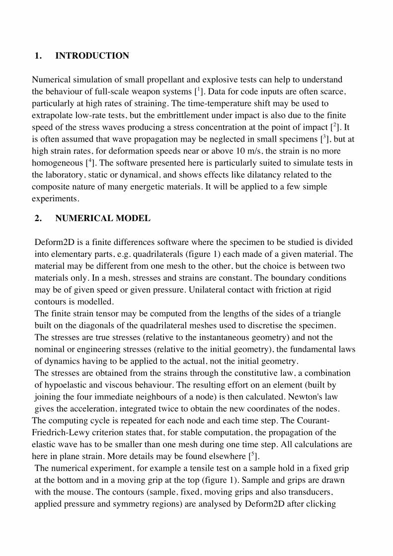
Numerical simulation of fracture in compression
Figure 4- Specimen shape at complete fracture. It is highly distorted as in a real material. One may
distinguish the contours of the fractured regions. The compression speed of 10 m/s makes the
deformation larger at the top of the specimen. The number of nodes is 200. The height of the sample
is 0.02 m for a width of 0.01 m. All other data are the same as in tension above (figure 2).
Str
ess
(M
Pa) 10
0
Dil
atat
ion (
%)
10Strain (%)
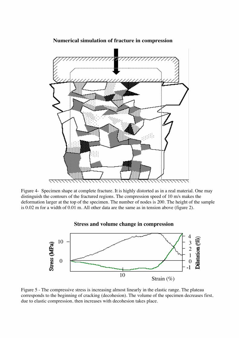
Stress and volume change in compression
-1-1 0 1
2 3
4
Figure 5 - The compressive stress is increasing almost linearly in the elastic range. The plateau
corresponds to the beginning of cracking (decohesion). The volume of the specimen decreases first,
due to elastic compression, then increases with decohesion takes place.

3.3. Comparison with experiment
The agreement with the experimental curves [6], [7] is not too bad. In tension, the
volume increases all the time, first linearly, as may be expected from Poisson’s ratio,
then much more rapidly than observed experimentally.
The maximum strain is much higher in compression than in tension as in most
materials. In compression, there is a decrease of the volume, due to elastic
compression, followed by an increase, due to decohesion, as observed experimentally.
4. WAVE PROPAGATION IN AN EXPLOSIVE SIMULANT
4.1. Numerical model
A 150 mm length and 10 mm thickness bar, made of an explosive simulant (the same
as above but entered in the software as an homogeneous material for the sake of
simplicity) is impacted at one end at a speed of 1 m/s during 100 µs. The variation of
the longitudinal stress at the other end is shown on figure 6.
Time (ms)
Str
ess
x 10
P
a4
Oscillations in an explosive simulant bar
1 2 3 4 5 6 7 8 9
0
1
2
3
4
5
6
-1
-2
-3
-4
-5
104 Moyenne sur capteur N° 1
ExperimentalNumerical
Figure 6 - Oscillations in a bar impacted at one end. The computed curve (in black) is compared with
the experimental curve (in gray)
4.2. Comparison with experiment

4.2.1. Experimental set-up
A 150 x 10 x 10 mm explosive simulant bar was equipped with an accelerometer
connected to an Apple II microcomputer with a data acquisition board. The bar was
impacted at one side with a pen and the signal from the accelerometer at the opposite
side was recorded.
4.2.2. Viscosity
The data from the numerical simulation (gray curve) agree with the experimental
results (black curve). They have been obtained with a viscosity of 1000 Pa.s. Hence
the viscosity for a solid composite explosive should be around this value. The
maximum measurable value during polymerization of composite solid propellants was
found to be of 106 Poises (105 Pa.s) [8] with a Brookfield viscosimeter. It is hundred
times smaller; the reason for the discrepancy is not clear. Unfortunately, practically no
information can be found on this subject in the literature. There are many papers about
viscoelasticity, but the results are expressed in terms of damping or relaxation times.
The logarithmic decrement is found to be about 0.3 from the experimental data.
4.2.3. Speed of sound
The longitudinal wave speed is found to be of 270 m/s for assumed speeds of 810 and
140 m/s respectively for longitudinal and transverse waves (the material is taken as
homogeneous here). With the classical formula for bar wave speed one finds 235 m/s.
5. WAVE PROPAGATION IN GUN POWDER
5.1. Numerical model
In the numerical experiment, two transducers are simulated in the gunpowder bed at
its top and at its bottom, on order to “measure” the speed of an elastic wave.
The powder bed has two constituents, nitrocellulose (reinforcement) and air (matrix).
The elastic modulus of the solid phase is taken as 1.5 GPa, with a Poisson’s ratio of
0.45 and a density of 1600 kg/m3. The global density is 850 kg/m3. The height of
powder is 0.05 m. The impact speed is 0.1 m/s, for a duration of 20 µs. The geometry
of the numerical experiment is shown on figure 7. The non-linearities due to contact
between the grains are not taken into account.
The computed recordings of the longitudinal stress at top and bottom of the powder
bed are given on figure 8. From these one obtains the propagation time of the pulse
from top to bottom.

Transducer n° 2
Transducer n° 1
Simulated gunpowder
grains
Moving anvil
ContainerP
ropagati
on d
ista
nce
Betw
een
tra
nsd
ucers
1 a
nd
2
Numerical experiment of wave propagation in a powder bed
Figure 7 - Numerical experiment for simulating a wave propagation in a powder bed.
The powder is contained in a container and compressed by a moving anvil. Two regions (dotted line)
at the top and bottom simulate transducers for recording the stress as a function of time.
The stresses in the “transducers” are the mean stress in the regions defined by the contours that may
be seen near the top and bottom of the powder bed

Sigma yy (Pa)
Compression (déformation plane, Déform2D, 12/02/94 )
Déformable Mobile Fixex
0
0.1
0.01
-0.01
Str
ess
(MP
a)Propagation timeof the elastic wave
Transducer n° 1
Transducer n° 2
Simulated pulse propagation
Time (ms)
Figure 8 - The propagation time of the elastic wave is obtained from the delay between the computed
stress curves in the two “transducers”, e.g. 0.09 ms, corresponding to a wave speed of 400 m/s.
5.2. Comparison with experiment
Compression tests (figure 9) are performed in brass cylinders containing the powder.
The compression anvil receives an impact from a Charpy pendulum, generating a
pulse propagating through the powder bed. A quartz transducer detects the instant of
impact. A strain-gage transducer at the bottom detects the incoming wave pulse.
The signals from the two transducers are recorded with an oscilloscope. From the
delay between the records given by the two transducers the speed of the elastic wave is
obtained.

Quartz transducer
Copperanvil
Load cell
Oscilloscope
Charpy pendulum
Gunpowder
Experimental set-up for measuring wave speed in a powder bed
Figure 9 - Experimental set-up for measuring wave speed in a powder bed. An impact of known
energy is obtained with a Charpy pendulum. The effort is recorded on top with a quartz transducer
and on bottom with a strain-gage transducer. Both signals are recorded on an oscilloscope. The wave
speed is obtained from the delai between the two signals.
The speed of the wave varies between 179 and 354 m/s, depending on the weight and
falling height of the Charpy impacter, the prestress, the height of the powder bed
(figure 10). The speed given by the numerical simulation, 400 m/s, is higher than all
the experimental values, which may be due to the contact non-linearities between the
grains, not taken into account in the simulation.
Using the Schubert formula [9] one finds 240 m/s, with a Young’s modulus of 1.5 GPa
and a Poisson’s ratio of 0.45 for the nitrocellulose, the porosity of the bed being 40 %.
The assumptions are the same used by Schubert, e.g. radius of curvature at the contact
point equal to the grain radius and a tension of 1 kPa.

Effect of impactor, prestress and height on elastic wave speed in
a powder bed
Wave speed (m/s)
0,01
0,1
1
10
100
170 220 270 320 370
Impactor Falling height Prestress Height ofpowder
Figure 10 - The speed of the wave increases when the energy of the impactor (weight and falling
height) increases and when the height of powder and prestress decreases. The software is not
sophisticated enough to predict such effects.
6. CONCLUSION
The computed curves of the deformation (stress and dilatancy) are qualitatively in
accord with experiment for highly filled elastomers. Volume is always increasing in
tension and, in compression, a decrease is followed by an increase due to decohesion.
The software shows how oscillations are generated in a composite explosive simulant
bar by an impact. The study of the corresponding wave propagation shows the
influence of viscosity, a parameter often cited in rheological studies but to which a
numerical value is rarely given. The damping of the oscillations corresponds to a
viscosity 100 times smaller than measured directly towards the end of polymerization
of a composite propellant. The propagation speed of an elastic wave in a powder bed is
reasonably in accord with experimental results although the contact phenomena were
not modelled.
Deform2D is a simple tool to understand the static and dynamical behaviour of
energetic materials. It may be useful to optimize an experimental program or a more
sophisticated numerical simulation with a standard software. It appears the necessity of
knowing the mechanical properties of not only the composites but also of their
components (binder and crystalline phase). The same is valid for gun powder where
one should determine the mechanical properties (static and dynamic) of the powder
material and of the powder bed.
7. REFERENCES
[1] Duffy K.P., Baker P.J., Barr E.J., Mellor A.M., Dynamic analysis of drop weight impact rocket
propellant ignition, AIAA-91-2193-CP, 1991.
[2] Schaeffer B., Simulation numérique sur microordinateur du comportement et de la rupture à
grande vitesse de déformation. J. de Physique IV, Colloque C3, suppl. III, vol 1, Oct. 1991, pp. 707-
712.
[3] Stelly, M., Comportement mécanique des matériaux sollicités à grande vitesse, Matériaux et
Techniques, Novembre-Décembre 1986, p. 485.
[4] Bainville D., Maillot D., Essais mécaniques sur matériau agrégataire aux vitesses intermédiaires,
J. de Physique IV, , suppl. au n° 8, t. 46, Colloque C5-469, août 1985, pp.469-474.
[5] Schaeffer B., DEFORM2D: Microcomputer simulation of behaviour and fracture of solid parts
using numerical methods, FEMCAD 88, Paris, 17-19 oct 1988, vol. 1, pp. 133-142.
[6] Schaeffer B., Rhéologie des explosifs composites, ICT Jahrestagung 1980, pp. 599-611.
[7] Lebois J., Massat H, Définition d’un critère de pseudo-plasticité associé à un critère de rupture,
ICT Jahrestagung 1980, pp. 687-698.
[8] Schaeffer B., Rhéologie des propergols en cours de polymérisation. Ind. Min., No spécial
Rhéologie, t. IV, N° 5, 15 Nov. 1977.
[9] Gregor W., Rumpf H., Velocity of sound in two-phase media, Int. J. Multiphase Flow, Vol. 1,
1975, pp. 753-769.
Related Documents