Nonparametric Frontier Estimation: a Robust Approach * Catherine Cazals IDEI/GREMAQ Universit´ e de Toulouse Jean-Pierre Florens IDEI/GREMAQ Universit´ e de Toulouse L´ eopold Simar † Institut de Statistique Universit´ e Catholique de Louvain January 3, 2001 Abstract A large amount of literature has been developed on how to specify and to estimate production frontiers or cost functions. Two different approaches have been mainly de- veloped: the deterministic frontier model which relies on the assumption that all the observations are on a unique side of the frontier, and the stochastic frontier models where observational errors or random noise allows some observations to be outside of the frontier. In a deterministic frontier framework, nonparametric methods are based on envelopment techniques known as FDH (Free Disposal Hull) and DEA (Data Envel- opment Analysis). Today, statistical inference based on DEA/FDH type of estimators is available but, by construction, they are very sensitive to extreme values and to outliers. In this paper, we build an original nonparametric estimator of the “efficient frontier” which is more robust to extreme values, noise or outliers than the standard DEA/FDH nonparametric estimators. It is based on a concept of expected minimum input function (or expected maximal output function). We show how these functions are related to the efficient frontier itself. The resulting estimator is also related to the FDH estimator but our estimator will not envelop all the data. The asymptotic theory is also provided. Our approach includes the multiple inputs and multiple outputs cases. As an illustration, the methodology is applied to estimate the expected minimum cost function for french post offices. Keywords: production function, cost function, expected maximum production function, expected minimum cost function, frontier, nonparametric estimation. JEL Classification: C13, C14, D20. * This paper is a revised version of Cazals and Florens (1997). † Visiting IDEI, Toulouse with the support of the Minist` ere de l’Education nationale , de la recherche et de la technologie, France. Research support from “Projet d’Actions de Recherche Concert´ ees” (No. 98/03–217) from the Belgian Government is also acknowledged.

Welcome message from author
This document is posted to help you gain knowledge. Please leave a comment to let me know what you think about it! Share it to your friends and learn new things together.
Transcript

Nonparametric Frontier Estimation: a Robust Approach∗
Catherine Cazals
IDEI/GREMAQUniversite de Toulouse
Jean-Pierre Florens
IDEI/GREMAQUniversite de Toulouse
Leopold Simar†
Institut de Statistique
Universite Catholique de Louvain
January 3, 2001
Abstract
A large amount of literature has been developed on how to specify and to estimateproduction frontiers or cost functions. Two different approaches have been mainly de-veloped: the deterministic frontier model which relies on the assumption that all theobservations are on a unique side of the frontier, and the stochastic frontier modelswhere observational errors or random noise allows some observations to be outside ofthe frontier. In a deterministic frontier framework, nonparametric methods are basedon envelopment techniques known as FDH (Free Disposal Hull) and DEA (Data Envel-opment Analysis). Today, statistical inference based on DEA/FDH type of estimatorsis available but, by construction, they are very sensitive to extreme values and tooutliers.
In this paper, we build an original nonparametric estimator of the “efficient frontier”which is more robust to extreme values, noise or outliers than the standard DEA/FDHnonparametric estimators. It is based on a concept of expected minimum input function(or expected maximal output function). We show how these functions are related tothe efficient frontier itself. The resulting estimator is also related to the FDH estimatorbut our estimator will not envelop all the data. The asymptotic theory is also provided.Our approach includes the multiple inputs and multiple outputs cases.
As an illustration, the methodology is applied to estimate the expected minimumcost function for french post offices.
Keywords: production function, cost function, expected maximum production function,expected minimum cost function, frontier, nonparametric estimation.
JEL Classification: C13, C14, D20.
∗This paper is a revised version of Cazals and Florens (1997).†Visiting IDEI, Toulouse with the support of the Ministere de l’Education nationale , de la recherche et de
la technologie, France. Research support from “Projet d’Actions de Recherche Concertees” (No. 98/03–217)from the Belgian Government is also acknowledged.

1 Introduction
Since the basic work of Koopmans (1951) and Debreu (1951) on activity analysis, a large
amount of literature has been developed on how to specify and to estimate production
frontiers or cost functions and on how to measure technical efficiency of production units. See
Shephard (1970) for a modern economic formulation of the problem. Consider a production
technology where the activity of production units is characterized by a set of inputs x ∈ IRp+
used to produce a set of outputs y ∈ IRq+.
The production set is defined as the set
Ψ = {(x, y) ∈ IRp+q+ | x can produce y}. (1.1)
This set can be described mathematically by its sections. For example, in the input space
we have the input requirement sets defined for all y ∈ Ψ as C(y) = {x ∈ IRp+ | (x, y) ∈ Ψ}.
The radial (input-oriented) efficiency boundary (“efficient frontier”) is then defined by:
∂C(y) = {x | x ∈ C(y), θx /∈ C(y) ∀ 0 < θ < 1}. (1.2)
The Farrell input measure of efficiency of a production unit working at level (x0, y0) is then
defined as:
θ(x0, y0) = inf{θ | θx0 ∈ C(y0)} = inf{θ | (θx0, y0) ∈ Ψ}. (1.3)
Note that ∂C(y) = {x | θ(x, y) = 1}.
The same could be done in the output space where the output requirement set is defined
for all x ∈ Ψ as P (x) = {y ∈ IRq+ | (x, y) ∈ Ψ}. Its radial efficient boundary is then:
∂P (x) = {y | y ∈ P (x), λy /∈ P (x) ∀ λ > 1}. (1.4)
Then the Farrell output measure of efficiency for a production unit working at level (x0, y0)
is defined as
λ(x0, y0) = sup{λ | λy0 ∈ P (x0)} = sup{λ | (x0, λy0) ∈ Ψ}. (1.5)
Here, ∂P (x) = {y | λ(x, y) = 1}.
Note that the frontier of Ψ is unique and ∂C(y) and ∂P (x) are two different ways of de-
scribing it. Different assumptions can be assumed on Ψ like free disposability1 or convexity,...
(see, e.g., Shephard, 1970 for details).1Free disposability in inputs and outputs of Ψ means that if (x, y) ∈ Ψ then (x′, y′) ∈ Ψ for any x′ ≥ x
and y′ ≤ y, where inequality between vectors has to be understood element by element.
1

The econometric problem is thus how to estimate Ψ from a random sample of production
units {(Xi, Yi) | i = 1, . . . , n}. Two different approaches have been mainly developed: the
deterministic frontier model which relies on the assumption that the DGP (Data Generating
Process) is such that Prob((Xi, Yi) ∈ Ψ) = 1, and the stochastic frontier models where
observational errors or random noise allows some observations to be outside of Ψ.
In a deterministic frontier framework, nonparametric methods have known an increasing
success since the pioneering work of Farrell (1957). The methods are based on envelopment
techniques known as FDH (Free Disposal Hull) estimators initiated by Deprins, Simar and
Tulkens (1984) which rely only on free disposability assumptions for Ψ and DEA (Data
Envelopment Analysis) estimators, which assumes free disposability and convexity of Ψ, ini-
tiated by Farrell and operationalized as linear programming estimators by Charnes, Cooper
and Rhodes (1978). They can be defined as follows: the FDH estimator of Ψ is the free
disposal hull of the set of observations:
ΨFDH ={
(x, y) ∈ IRp+q+ |y ≤ Yi, x ≥ Xi, i = 1, . . . , n
}.
Then the convex hull of ΨFDH provides the DEA estimator of Ψ:
ΨDEA = {(x, y) ∈ IRp+q+ |y ≤
n∑
i=1
γiYi ; x ≥n∑
i=1
γiXi for (γ1, . . . , γn)
such thatn∑
i=1
γi = 1 ; γi ≥ 0, i = 1, . . . , n}.
It is the smallest free disposal convex set covering all the data.
Nonparametric envelopment estimators have been extensively used for estimating effi-
ciency of firms (see Seiford, 1996, for a nice survey). Today, statistical inference based on
DEA/FDH type of estimators is available either by using asymptotic results (Kneip, Park
and Simar, 1998 and Park, Simar and Weiner, 2000) or by using the bootstrap, see Simar
and Wilson (2000) for a recent survey of the available results. Nonparametric deterministic
frontier models are very appealing because they rely on very few assumptions but it is known
that by construction, they are very sensitive to extreme values and to outliers.
In a stochastic frontier framework, where noise is allowed, only parametric restrictions
on the shape of the frontier and on the DGP allow identification of noise from efficiency
and estimation of the frontier. Most of the available techniques are based on the maximum
likelihood principle, in the spirit of the work of Aigner, Lovell and Schmidt (1977) and
Meeusen and van den Broek (1977).
Our work is a part of the literature of nonparametric frontier estimation in that we
build an original nonparametric estimator of the “efficient frontier” which is more robust to
extreme values, noise or outliers than the standard DEA/FDH nonparametric estimators.
2

To the best of our knowledge, very few methods are proposed in the literature to address
this important issue. Wilson (1993) and (1995) has proposed descriptive methods to detect
outliers in this framework. This paper proposes robust estimators of frontiers with their full
statistical treatment.
For sake of simplicity, we will make our presentation in the input-oriented framework,
where we have one input x (p = 1) and q outputs y. The input efficient frontier can then
be interpreted as a “minimum input function” or as a “minimum cost function”. We will
indicate, in Appendix A, how to make the changes for the output-oriented case where we
have one output y (q = 1) and p inputs x: in this case, the efficient frontier is a “maximum
production function”. A shown later, a complete multivariate extension (multi-input and
multi-output cases) is also possible.
We will define a concept of expected minimum input function (or expected minimum cost
function) and present the methodology for a nonparametric estimation of it. The output
oriented case provides the concept of expected maximum production function. We show
how these functions are related to the efficient frontier defined above under the hypothesis
of free disposability. The resulting estimator is also related to the FDH estimator but our
estimator will not envelop all the data. The method can also be adapted if, in addition, the
assumption of convexity of Ψ is made and convex estimators of Ψ are wanted. In this case,
our estimator will be related to the DEA estimator.
The paper is organized as follows. Section 2 presents the basic concepts of expected
minimum input function and its relation to frontiers. Section 3 proposes a nonparametric
estimator and analyses its asymptotic properties and its relations with other nonparametric
estimators. In Section 4, a numerical illustration is proposed: the methodology is applied
to estimate the expected minimum cost function for french post offices. We use a data set
on labor (as input) and mail volumes (as output) on around 10.000 post offices. Section
5 suggests some two useful extensions: how to introduce exogenous explanatory variables
in the model and how to generalize the approach to the multivariate case (multi-input and
multi-output). Section 6 concludes.
2 The Expected Minimum Input Function
Let us consider a random vector (X, Y ) on IR+× IRq+. The first element X is the input and
the q-dimensional vector Y represents the outputs. The joint distribution on (X, Y ) defines
the production process. Such probability measure is usually decomposed into a marginal
distribution on Y and a conditional distribution on X given Y = y.
In this paper, we will rather concentrate on an other characterization of the joint proba-
3

bility measure on (X, Y ): the joint survivor function. Let us denote by Y ≥ y the property
that Yj ≥ yj for j = 1, . . . , q. We will consider the conditional probability measure on X
given Y ≥ y. If the joint probability measure is characterized by the joint survivor function:
S(x, y) = Prob(X ≥ x, Y ≥ y), (2.1)
the conditional distribution on X given Y ≥ y may be described by its survivor function:
Sc(x | y) = Prob(X ≥ x | Y ≥ y) (2.2)
=S(x, y)
SY (y), (2.3)
where SY (y) = S(0, y) = Prob(Y ≥ y) denotes the marginal survivor function of Y . It is
supposed here and below that SY (y) 6= 0 or that y is an interior point of the support of the
marginal distribution of Y .
The lower boundary of the support of the conditional distribution whose survivor function
is Sc(x | y) is given by the function:
ϕ(y) = inf{x | Sc(x | y) < 1}. (2.4)
This function is monotone non decreasing in y as shown by the following theorem:
Theorem 2.1 The frontier function ϕ(y) is monotone non decreasing in y:
For all y′ ≥ y we have ϕ(y′) ≥ ϕ(y). (2.5)
Proof:
ϕ(y) = inf{x | Sc(x | y) < 1}= sup{x | Sc(x | y) = 1}.
Denote Ay the set {x | Sc(x | y) = 1}. We have
Ay = {x | Prob(X ≥ x | Y ≥ y) = 1}= {x | Prob(X < x | Y ≥ y) = 0}= {x | Prob(X < x, Y ≥ y) = 0}.
If y′ ≥ y, Ay ⊆ Ay′ , then sup{x | x ∈ Ay′} ≥ sup{x | x ∈ Ay} which completes the proof.
Note that this minimum input (or cost) frontier function ϕ(y) is always defined and
monotone non decreasing: no particular assumption on Ψ are needed. By construction and
from the preceding theorem, ϕ(y) is the largest monotone function which is smaller than
4

∂C(y) the input-efficient frontier of Ψ (remember that here p = 1). It is clear that if the
attainable set Ψ is free disposal, ∂C(y) is monotone and coincides with ϕ(y).
Consider now an integer m ≥ 1 and let (X1, . . . , Xm) be m independent identically
distributed random variables generated by the distribution of X given Y ≥ y.
Definition 2.1 The expected minimum input function of order m denoted by ϕm(y) is the
real function defined on IRq+ as
ϕm(y) = E(min(X1, . . . , Xm) | Y ≥ y), (2.6)
where we assume the existence of this expectation.
The function ϕm(y) can be computed as follows.
Theorem 2.2 If ϕm(y) exists, it is given by
ϕm(y) =∫ ∞
0[Sc(u | y)]m du. (2.7)
Proof: This result is an elementary consequence of the rules of integration by parts, since
if Xmin = min(X1, . . . , Xm), we have:
Prob(Xmin ≥ u | Y ≥ y) = [Sc(u | y)]m, (2.8)
from which the result derives.
From its definition, it is clear that for any y fixed, ϕm(y) is a decreasing function of m.
The limiting case when m→∞ is of particular interest. It achieves the efficient frontier:
Theorem 2.3 For any fixed value of y we have
limm→∞ϕm(y) = ϕ(y). (2.9)
Proof:
ϕm(y) =∫ ∞
0[Sc(u | y)]m du
=∫ ϕ(y)
0[Sc(u | y)]m du+
∫ ∞
ϕ(y)[Sc(u | y)]m du.
For all u ≤ ϕ(y), Sc(u | y) = 1. So that
ϕm(y) = ϕ(y) +∫ ∞
ϕ(y)[Sc(u | y)]m du. (2.10)
5

For u > ϕ(y), Sc(u | y) < 1, so [Sc(u | y)]m tends to zero when m→∞. Using the Lebesgue
convergence theorem, the integral on the right hand side of (2.10) converges to zero when
m→∞ giving the result.
The function ϕm(y) converges to a monotone non decreasing function ϕ(y) as m → ∞,
but it is not monotone non decreasing itself unless we add the following assumption.
Assumption 2.1 The conditional distribution of X given Y ≥ y has the following property
For all y′ ≥ y, Sc(x | y′) ≥ Sc(x | y). (2.11)
This assumption is not needed for all the results of this paper except the next theorem, but
it appears to be quite reasonable: it says that the chance of spending more than an input
(or cost) x does not decrease if a firm produces more. So, if we want a joint survival function
S(x, y) to represent a production process, Assumption 2.1 is quite natural. It also implies
the monotonicity of ϕm(y):
Theorem 2.4 Under Assumption 2.1, ϕm(y) is monotone non decreasing in y.
Proof: This is immediate by the expression of ϕm(y) given in Theorem 2.2 and from prop-
erties of integrals.
From an economic point of view, the expected minimum input (cost) function of order
m, ϕm(y) has its own interest: it is not the efficient frontier of the production set but it
might be useful in term of practical efficiency analysis. Suppose a production unit produces
a quantity of output y0 using the quantity x0 of input, ϕm(y0) gives the expected minimum
cost among a fixed number of m potential firms producing more than y0. For this particular
unit, working at level (x0, y0), it is certainly worth to know this value because it gives a clear
indication of how efficient he is compared with these m potential units. This is achieved by
comparing its own level x0 with the “benchmarked” value ϕm(y0). At this stage, m could be
any number from 1 to∞. In practice, a few values of m could be used to guide the manager
of the production unit to evaluate its own performance.
But the most attractive property of this function is that it can be easily non parametri-
cally estimated without the drawbacks of the methods trying to estimate the frontier itself:
it will be less sensitive to noise, extreme values or outliers. This is developed in the next
section.
In Appendix A, we indicate how the concepts and properties can be adapted to the
output oriented case with one output y and p inputs x.
6

3 Nonparametric Estimation
Consider, for simplicity an i.i.d. sample (xi, yi), i = 1 . . . , n of the random vector (X, Y ).
The empirical survivor function is defined by:
Sn(x, y) =1
n
n∑
i=1
1I(xi ≥ x, yi ≥ y). (3.1)
The empirical version of Sc(x | y) is then given by:
Sc,n(x | y) =Sn(x, y)
SY,n(y), (3.2)
where SY,n(y) = (1/n)∑ni=1 1I(yi ≥ y). Note that this estimator does not require any smooth-
ing procedure as required when the conditional distribution of X given Y = y is required.
All the properties of ϕ(y) and ϕm(y) of the preceding section remain valid when the
function Sc(x | y) is replaced by Sc,n(x | y). In particular we have the lower boundary of
the support of the empirical conditional distribution characterizing the estimated efficient
frontier of the production set. It is given by the function:
ϕn(y) = inf{x | Sc,n(x | y) < 1}. (3.3)
This function is monotone non decreasing in y. It is the input oriented efficient frontier
obtained by the FDH estimator. The estimator of the expected minimum input function of
order m is defined by:
ϕm,n(y) = E(min(X1, . . . , Xm) | Y ≥ y), (3.4)
where X1, . . . , Xm are m i.i.d. random variables generated by the empirical distribution of
X given Y ≥ y whose survivor function is Sc,n(x | y). It is computed through
ϕm,n(y) =∫ ∞
0[Sc,n(u | y)]m du. (3.5)
The relation (2.10) between ϕm(y) and ϕ(y) remains valid with their empirical versions:
ϕm,n(y) = ϕn(y) +∫ ∞
ϕn(y)[Sc,n(u | y)]m du, (3.6)
from which we obtain again that for all y,
limm→∞ ϕm,n(y) = ϕn(y). (3.7)
So, our estimator of the expected minimum input function of order m converges to the
FDH input efficient frontier when m increases. In particular, in finite samples, it should be
noticed that, even when m = n, our estimator is different from the FDH estimator:
ϕn,n(y) 6= ϕn(y).
7

Even for large finite values of m, the estimator ϕm,n(y) is less sensitive to extremes values
than the FDH estimator ϕn(y) which by construction, envelopes all the observations. The
asymptotic theory is discussed below. Note also that ϕm,n(y) is not necessarily monotone
non decreasing. Indeed, even if Assumption 2.1 is assumed for the true conditional survivor
function, it could not be verified by its empirical counterpart. Of course we know that for
large sample size n, it will mostly be the case.
The integral in (3.5) defining our estimator may be easily computed in practice. Let n(y)
be the number of observations of yi greater or equal to y, i.e. n(y) =∑ni=1 1I(yi ≥ y), and,
for j = 1, . . . , n(y), denote by xy(j) the j-th order statistic2 of the observations xi such that
yi ≥ y: xy(1) < xy(2) < . . . < xy(n(y)).
The function Sc,n(u | y) is a step function such that:
Sc,n(u | y) = 1 if u ≤ xy(1)
=n(y)− jn(y)
if xy(j) < u ≤ xy(j+1)
= 0 if u > xy(n(y)).
Then we have:
ϕm,n(y) = xy(1) +n(y)−1∑
j=1
[n(y)− jn(y)
]m(xy(j+1) − xy(j)). (3.8)
The following theorem summarizes the asymptotic properties of our estimator for any
fixed value of m.
Theorem 3.1 Assume that Ψ, the support of the random vector (X, Y ) is compact, then
for any interior point y in the support of the Y distribution, and for any m ≥ 1:
(i) ϕm,n(y)→ ϕm(y) a.s. as n→∞ ;
(ii) L (√n(ϕm,n(y)− ϕm(y)))→ N(0, σ2(y)) as n→∞, where
σ2(y) = E
[m
SY (y)m
∫ ∞
0S(u, y)m−11I(X ≥ u, Y ≥ y) du− mϕm(y)
SY (y)1I(Y ≥ y)
]2
.
2We suppose here that there are no ties among the xy(j): this allow the simple formulation of Sc,n(u | y).
In case of ties, all the theory remains valid but the explicit expression of ϕm,n(y) in (3.8) is no more valid.The general expression (3.5) has to be used.
8

Proof:
(i) This result follows from a strong law of large numbers which implies the almost sure
convergence of Sc,n(u | y) to Sc(u | y) and from the Lebesgue dominated convergence theorem
which warrants the convergence of the integrals defining ϕm,n(y) and ϕm(y).
(ii) The argument will follow the standard Delta method (see Serfling, 1980, Chapter 6,
Theorem A). Let us denote by
T (S) =∫ ∞
0[Sc(u | y)]m du.
T (S) is an operator which associates a real value to any survivor function S. This operator
is differentiable at the Frechet sense w.r.t. the sup norm, that is:
T (R)− T (S) = DTS(R− S) + ε(R− S)||R− S||, (3.9)
for any two survivor functions S and R, where the sup norm is used:
||V (x, y)|| = sup(x,y)∈Ψ
|V (x, y)|,
and where ε(V ) → 0 when ||V || → 0. The Frechet derivative is obtained by standard
calculus, noting that Sc(u | y) = S(u, y)/SY (y):
DTS(V ) =m
SY (y)m
∫ ∞
0S(u, y)m−1V (u, y) du−mϕm(y)
SY (y)V (0, y). (3.10)
Now, applying (3.9) and noting that DTS(Sn − S) = DTS(Sn) we have:
√n[T (S)− T (S)] =√n
n
n∑
i=1
[m
SY (y)m
∫ ∞
0S(u, y)m−1 1I(xi ≥ u, yi ≥ y) du− mϕm(y)
SY (y)1I(yi ≥ y)
]
+ε(Sn − S)(√n||Sn − S||). (3.11)
As√n||Sn − S|| = Op(1) by the Dvoretzky, Kiefer and Wolfowitz inequality (see Serfling,
1980, Chapter 2, Theorem A) and ε(Sn − S) → 0 in probability (because Sn is uniformly
convergent), the second term of the r.h.s. of (3.11) converges to 0. The theorem comes then
from a central limit theorem applied to the first term of the r.h.s. of (3.11). In particular, it
is easy to verify that the term between brackets has zero mean. Indeed:
E
[m
SY (y)m
∫ ∞
0S(u, y)m−1 1I(X ≥ u, Y ≥ y) du− mϕm(y)
SY (y)1I(Y ≥ y)
]
= n
[m
SY (y)m
∫ ∞
0S(u, y)m−1 S(u, y) du− mϕm(y)
SY (y)SY (y)
]= 0.
9
Note the√n rate of convergence of ϕm,n(y) to ϕm(y) which is rather unusual in nonpara-
metric statistics. The expression of the variance can be used to derive asymptotic confidence
intervals for ϕm(y): by plugging estimators for the unknown quantities and taking the empir-
ical mean for the expectation provides σ2(y), a consistent estimator of the variance. Observe
that for a given sample size, σ2(y) will increase with y.
Note that these convergence results may be improved by a functional limit theorem
which is given in Appendix B. With this functional theorem the asymptotic can be derived
for transformations of ϕm.
The result can also be extended to the analysis of the asymptotic properties of a vector
(ϕm,n(y1), . . . , ϕm,n(yr)). We still have the asymptotic r-variate normal distribution with
asymptotic covariances given by
Σk,` = Cov(ϕm,n(yk), ϕm,n(y`)) = E[Γ(yk, X, Y ) Γ(y`, X, Y )
], (3.12)
where
Γ(y,X, Y ) =m
SY (y)m
∫ ∞
0S(u, y)m−11I(X ≥ u, Y ≥ y) du− mϕm(y)
SY (y)1I(Y ≥ y).
The issue of how to choose m in practice has been discussed above in Section 2. We
know that the estimator ϕm,n(y) converges to the FDH estimator ϕn(y) defined in (3.3) as
m → ∞. But we know also from Park, Simar and Weiner (2000), that under regularity
conditions, as n → ∞, the FDH estimator ϕn(y) converges to the true unknown frontier
ϕ(y) defined in (2.4).
The value of m can thus be viewed as a “trimming” or “smoothing” parameter and the
natural question then arises: how to define m as a function of n such that ϕm,n(y) converges
to ϕ(y), as n → ∞. This could also give some insights on how to choose m in practice in
order to obtain a consistent estimator of the true frontier, if wanted. The result follows from
the next theorem.
Theorem 3.2 Assume that the joint probability measure of (X, Y ) on the compact support
Ψ provides a strictly positive density on the frontier ϕ(y) and that the function ϕ(y) is
continuously differentiable in y. Then, for any y interior to the support of Y we have:
L(n1/(1+q)(ϕmy(n),n(y)− ϕ(y))
)→Weibull(µ1+q
y , 1 + q) as n→∞, (3.13)
where my(n) = O(β n log(n)SY (y)), with β > 1/(1 + q) and µy is a constant.
10

Proof: From Park, Simar and Weiner (2000) we know that
L(n1/(1+q)(ϕn(y)− ϕ(y))
)→Weibull(µ1+q
y , 1 + q) as n→∞,
where the parameter µy of the Weibull depends on local properties of the DGP near the
frontier point (ϕ(y), y). Now using (3.6) we obtain:
n1/(1+q)(ϕm,n(y)− ϕ(y)) = n1/(1+q)(ϕn(y)− ϕ(y)) + n1/(1+q)∫ ∞
ϕn(y)[Sc,n(u | y)]m du.
So the question is to find the value of m = my(n) such that the last term of the preceding
expression is op(1) as n → ∞. Using a mean value theorem, we can write the integral
as (xy(n(y)) − xy(1))[Sc,n(u | y)]m where u ∈ ]xy(1), xy(n(y))[. Since the support of (X, Y ) is
compact, the range of X is bounded, in addition, for u > ϕn(y), Sc,n(u | y) is bounded by
(n(y)− 1)/n(y). So to achieve our goal, it is sufficient that my(n) is such that
[(n(y)− 1)/n(y)]my(n) = Op(n−β),
where β > 1/(1 + q). Now, since log(1 − 1/n(y)) � −1/n(y) and n(y) � nSY (y) this is
equivalent to
my(n) = O(β n log(n)SY (y)),
with β > 1/(1 + q).
In practice, if a consistent estimator of the frontier itself is wanted, we might plug the
value of SY (y) in the formula to get an idea of the order of my(n), but of course the result
is only an asymptotic one.
Note that we loose the√n-consistency because here we use ϕm,n(y) to estimate the
frontier ϕ(y) itself and not ϕm(y), the “order-m” frontier which can be viewed as a “trimmed”
frontier.
Remark 3.1 Convexifying the estimator: Robust DEA estimator
The above results do not rely on convexity assumption regarding the attainable set Ψ. If Ψ
is convex, our estimator remains consistent with the same asymptotics but a convex esti-
mates of Ψ is obtained by convexifying the set above the obtained frontier ϕm,n(y). This
could be achieved by running a input-oriented DEA linear program on the set of points
{(ϕm,n(yi), yi), i = 1, . . . , n}. Again the obtained estimator will converge to the DEA frontier
estimator if m→∞, but, for finite m, it will not envelop all the data points.
11

4 Empirical Illustration
To illustrate our methodology, we analyze the production of the postal services in France.
More precisely, we focus on the cost of the delivery activity.
We use a cross-section data set of around 10.000 post offices, observed in 1994. We have
information about labor used and mail volumes for the delivery activity of each post office.
So, in this example, we have one input X and one output Y .
For each post office i, the variable Xi is the labor cost, which represents more than 80%
of the total cost of the delivery activity. It is measured by the quantity of labor. The output
Yi is defined as volume of the delivered mail (in number of objects). The data and the results
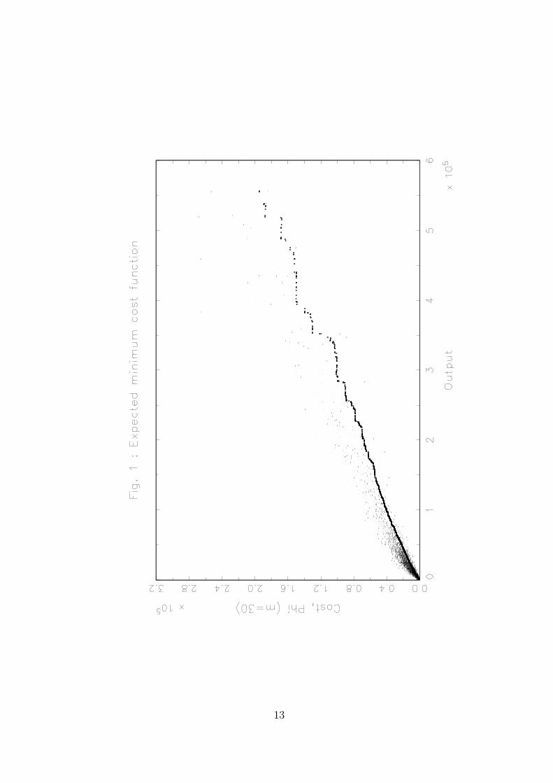
are shown in Figures 1–3.
Figure 1 plots the observed data, the cost xi (vertical axis) against the output yi (horizon-
tal axis), along with the nonparametric estimation of the expected minimum cost function
of order m: ϕm,n(y). Here the value of m was fixed to 30. Figure 2 zooms in Figure 1 for
the 3.000 first observations with the smallest output levels. It appears more clearly, in the
zoom, that the estimates is typically monotone and that many points stay outside (below)
the frontier of order m = 30.
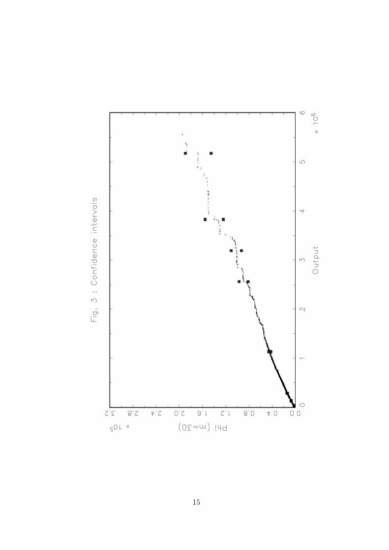
We have also estimated the variance function σ2(y) given in Theorem 3.1. This allows
to determine for some given points y confidence intervals. Figure 3 plots the pointwise
confidence intervals for a selected grid of points y. As expected, the lengths of the confidence
intervals increases when y is larger.
The FDH cost efficient frontier would envelop all the data points and is, of course, below
our estimate. Our obtained expected minimum cost of order m can thus be viewed as a
mark of “good practice” for producing units when studying their performance. However,
this benchmark is less “severe” than the FDH frontier because it is less sensitive to extreme
points.
With m = 30, 73% of the observations where used to determine the expected minimum
cost estimate of order m and so 27% of points were left out. Figure 4 indicates how the
percentage of points below the expected minimum cost estimate of order m decreases with
m. We notice that, in our example, this percentage is very stable from m = 50 where
roughly 10% of the observations are left out. These observations should be analyzed in
details because they are really extreme and could be outlying or perturbed by noise.
12
13

14
15

16

5 Extensions
5.1 Introducing environmental factors
The analysis of the preceding section can easily be extended to the case where additional
information is provided by other variables Z ∈ IRk, exogenous to the production process
itself, but which may explain part of it. It could be environmental variables, not under the
control of the manager. For instance, in the case of our empirical illustration above, we
could consider a variable Z representing the geographical density of the distribution area
of a post office (the number of delivery points by unit of length of the distribution route).
This variable, at least in the short term, is not under the control of the managers of the post
office but might influence the cost of the post office.
One way for introducing in the model this additional information is to condition the
production process to a given value of Z. Then, in the empirical example of the post offices,
we could study the expected minimum cost function for a post office delivering a mail volume
greater than y, with a geographical density equal to z.
Here, the joint survival function is written as S(x, y, z) = Prob(X ≥ x, Y ≥ y, Z ≥ z).
Then the methodology can be adapted by replacing in Section 2, Sc(x | y) by Sc(x | y; z)
where
Sc(x | y; z) = Prob(X ≥ x | Y ≥ y, Z = z) =∂zS(x, y, z)
∂zS(0, y, z), (5.1)
∂z denoting the operator of derivative of order k with respect to all the components of z:
∂z =∂k
∂z1 . . . ∂zk.
The estimation of this conditional survivor function will require a smoothing technique in z.
For example we will estimate S(x, y | Z = z) by:
Sn(x, y | Z = z) =
n∑
i=1
1I(xi ≥ x, yi ≥ y)K(z − zihn
)
n∑
i=1
K(z − zihn
) , (5.2)
where K(·) is a kernel and hn is the smoothing bandwidth which has the appropriate size for
getting the asymptotic theory. It can be shown that the resulting estimator of the mth order
expected minimum cost will achieve the rate of convergence√nhkn where k is the dimension
of Z. The theory can be developed in a similar way as in the preceding sections. We sketch
below the main points of the argument.
17

We want to estimate the conditional mth order expected minimum cost function defined
as
ϕm(y, z) =∫ ∞
0[Sc(u | y; z)]mdu, (5.3)
where
Sc(u | y; z) = Prob(X ≥ u | Y ≥ y, Z = z).
The estimator is given by:
ϕm,n(y, z) =∫ ∞
0
n∑
i=1
1I(xi ≥ u, yi ≥ y)K(z − zihn
)
n∑
i=1
1I(yi ≥ y)K(z − zihn
)
m
du. (5.4)
The asymptotic distribution of the estimator, with y and z fixed may be derived from the
general results of Ait-Sahalia (1995). Under regularity conditions on the distribution of Z
(continuous differentiable density function), if the kernel K(·) is symmetric and positive and
with the usual conditions on the bandwidth implying asymptotic normality and unbiasedness
of the estimator of the density of Z (i.e. nhkn → ∞ and nhk+4n → 0 as n → ∞), we obtain
that
L(√
nhkn(ϕm,n(y, z)− ϕm(y, z))→ N(0, σ2(y, z)fZ(z)
∫K2), (5.5)
with
σ2(y, z) = Var(A(X, Y ; y, z) | Z = z),
where
A(X, Y ; y, z) =m
[∂z(S(0, y, z))]m
∫ ∞
0[∂z(S(u, y, z))]m−11I(X ≥ u, Y ≥ y)du
− mϕm(y, z)
∂z(S(0, y, z))1I(Y ≥ y).
Note again that E(A(X, Y ; y, z) | Z = z) = 0.
The main argument of the proof is similar to the developments in Theorem 3.1. In the
linearization of√nhkn(ϕm,n(y, z)−ϕm(y, z)), the analog of the leading term of (3.11) becomes
√nhkn
n
n∑
i=1
[m
[∂z(S(0, y, z))]m
∫ ∞
0[∂z(S(u, y, z))]m−11I(xi ≥ u, yi ≥ y)
1
hknK(z − zihn
)du
− mϕm(y, z)
∂z(S(0, y, z))1I(yi ≥ y)
1
hknK(z − zihn
)]
=
√nhkn
n
n∑
i=1
A(xi, yi; y, z)1
hknK(z − zihn
),
then, under the appropriate regularity conditions on the kernel, the standard theory applies.
18

5.2 Multivariate extensions
We consider here the setting of Section 1 where we have p inputs and q outputs. We continue
the presentation in the input-oriented case . The modifications for the formulation in the
output-oriented case are straightforward (see also Appendix A). The production process is
here described by the joint probability measure of (X, Y ) on IRp+ × IRq
+. The support of
(X, Y ) is the attainable set Ψ.
There are several ways for describing the frontier ∂C(y) when p ≥ 1. For any (x, y) ∈ Ψ,
we can indeed define, as in (1.3), the input efficiency measure of the point (x, y):
θ(x, y) = inf{θ | θx ∈ C(y)} = inf{θ | (θx, y) ∈ Ψ}.
For any output level y in the interior of the support of Y , we want to describe, as in Section
2, the efficient frontier. In the multi-inputs case, the input-efficient frontier can then either
be described through the efficiency measures, since , ∂C(y) = {x | θ(x, y) = 1} or through
the efficient level of the inputs which, for any x ∈ IRp+ is given by:
x∂(y) = θ(x, y) x. ∈ ∂C(y). (5.6)
So the frontier, for any (x, y), can be characterized either by θ(x, y) or by x∂(y). It is clear
that if Ψ is free disposal, y′ ≥ y ⇒ C(y′) ⊆ C(y), then, for any x, θ(x, y) and x∂(y) are non
decreasing in y and when p = 1, x∂(y) determines ϕ(y) as defined in Section 2.
For a given level of outputs y0 in the interior of the support of Y , consider now the m
i.i.d. random variables Xi, i = 1, . . . , m generated by the conditional p-variate distribution
function FX(x | y0) = Prob(X ≤ x | Y ≥ y0) and define the set:
Ψm(y0) = {(x, y) ∈ IRp+q+ | x ≥ Xi, y ≥ y0}. (5.7)
Then, for any x, we may define
θm(x, y0) = inf{θ | (θx, y0) ∈ Ψm(y0)}. (5.8)
Note that θm(x, y0) may be computed by the following formula:
θm(x, y0) = mini=1,...,m
{maxj=1,...,p
(Xji
xj
)}(5.9)
where aj denotes the jth component of a vector a.
The following definition is the multivariate extension of our minimum input function of
order m as defined in Section 2 for p = 1.
19

Definition 5.1 For any x ∈ IRp+, the expected minimum input level of order m denoted by
x∂m(y) is defined for all y in the interior of the support of Y as:
x∂m(y) = xE(θm(x, y) | Y ≥ y), (5.10)
where we assume the existence of the expectation.
The expected minimum level of inputs of order m may be computed as follows.
Theorem 5.1 If x∂m(y) exists, it is given by:
x∂m(y) = x∫ ∞
0(1− FX(ux | y))mdu. (5.11)
Proof: The conditional distribution of θm(x, y) is given by
P (θm(x, y) ≤ u | Y ≥ y) = P(
mini=1,...,m
{maxj=1,...,p
(Xji
xj)
}≤ u | Y ≥ y
)
= 1− P(
mini=1,...,m
{maxj=1,...,p
(Xji
xj)
}> u | Y ≥ y
)
= 1−[P(
maxj=1,...,p
(Xji
xj) > u | Y ≥ y
)]m
= 1−[1− P
(maxj=1,...,p
(Xji
xj) ≤ u | Y ≥ y
)]m
= 1−[1− P (X ≤ ux | Y ≥ y
)]m.
Now, we obtain
E(θm(x, y) | Y ≥ y) =∫ ∞
0(1− FX(ux | y))mdu , (5.12)
from which the theorem follows.
Here again, in this multivariate case, when m → ∞, the expected minimum input level
of order m converges to the efficient input level defining the frontier:
Theorem 5.2 For any value of x ∈ IRp+ and for any y in the interior of the support of Y
we have:
limm→∞x
∂m(y) = x∂(y). (5.13)
20

Proof: This comes immediately from (5.12) where the integral is computed on two intervals
of values for u:
E(θm(x, y) | Y ≥ y) =∫ θ(x,y)
0(1− FX(ux | y))mdu+
∫ ∞
θ(x,y)(1− FX(ux | y))mdu
= θ(x, y) +∫ ∞
θ(x,y)(1− FX(ux | y))mdu,
where the integral converges to zero as m→∞.
The nonparametric estimation of x∂m(y) is straightforward: we replace the true FX(· | y)
by its empirical version, FX,n(· | y). We have
θm,n(x, y) = E(θm(x, y) | Y ≥ y) (5.14)
=∫ ∞
0(1− FX,n(ux | y))mdu. (5.15)
where
FX,n(x | y) =
∑ni=1 1I(xi ≤ x, yi ≥ y)∑ni=1 1I(yi ≥ y)
.
Then, the estimator of the expected minimum input level of order m is given by:
x∂m,n(y) = x θm,n(x, y). (5.16)
Note that here, due to the multivariate nature of FX,n(x | y), there is no simple explicit
expression of θm,n(x, y). The easiest way to compute it is by Monte-Carlo simulations which
can be performed as follows.
For a given y, draw a sample of size m with replacement among these xi such that yi ≥ y
and denote this sample by (X1,b, . . . , Xm,b). Then compute θbm(x, y) as:
θbm(x, y) = mini=1,...,m
maxj=1,...,p
(Xji,b
xj
) .
Redo this for b = 1, . . . , B, where B is large. Then,
θm,n(x, y) ≈ 1
B
B∑
b=1
θbm(x, y). (5.17)
The empirical frontier, which envelopes all the data points, is given by the standard FDH
solution. For instance, the FDH input efficiency measure of any (x, y) is given by:
θn(x, y) = inf{θ | (θx, y) ∈ ΨFDH} , (5.18)
where ΨFDH is defined in (1.6). It is computed through the following formula:
θn(x, y) = mini|yi≥y
{maxj=1,...,p
(xjixj
)}.
21

The corresponding estimated input-efficient level of inputs is given by:
x∂n(y) = x θn(x, y). (5.19)
The asymptotic developed in Section 3 for p = 1 remains valid, in particular, by Theorem
3.1, we still achieve the√n-consistency of x∂m,n(y) to x∂m(y) for m fixed as n→∞.
Note also, by (5.15), that
θm,n(x, y) = θn(x, y) +∫ ∞
θn(x,y)(1− FX,n(ux | y))mdu ,
so that θm,n(x, y)→ θn(x, y) as m→∞ for n fixed, or equivalently, the estimated minimum
input level of order m, x∂m,n(y) converges to the FDH efficient input level x∂n(y) when m→∞.
However, for a finite m our estimator does not envelop all the data points and is more robust
to extreme values, noise or outliers.
From Park, Simar and Weiner (2000) we know that the rate of convergence of the FDH
efficiency measures θn(x, y) to θ(x, y) is n1/(p+q), so Theorem 3.2 as to be adapted accordingly.
6 Conclusions
In this paper, we define a statistical concept of a production frontier and we propose a
nonparametric estimation of it. The concept is the expected minimum input level (or output
level) of order m. It can be applied in very general settings with multiple inputs and multiple
outputs. It is related to the usual FDH/DEA nonparametric envelopment estimators but
is more robust to extreme values, noise or outliers, in the sense that it does not envelop
all the data points. The estimator is easy to implement and the asymptotic properties
have been developed. In particular our estimator converges at a rate of√n to its population
counterparts. By choosing mn appropriately as a function of the sample size n, our estimator,
as an estimator of the frontier itself, recovers the asymptotic properties of the FDH estimator.
22

Appendix
A The Expected Maximal Production Function
We follow here, without any proofs, the development of Section 2 in the case we have one
output y and p inputs x. Here the production process is defined by the joint distribution
of the random vector (X, Y ) on IRp+ × IR+. We will concentrate here on the conditional
distribution of Y given X ≤ x. Let the joint distribution be
F (x, y) = Prob(X ≤ x, Y ≤ y), (A.1)
the conditional distribution on Y given X ≤ y is described by
Fc(y | x) = Prob(Y ≤ x | X ≤ x) (A.2)
=F (x, y)
FX(x), (A.3)
where FX(x) = Prob(X ≤ x).
The upper boundary of the support of Fc(y | x) is given by the function:
ψ(x) = sup{y | Fc(y | x) < 1}. (A.4)
This function is monotone nondecreasing in x. It is the smallest monotone nondecreasing
function which is greater or equal to the output-efficient frontier ∂P (x) as defined in Section
1. It is clear that if the attainable set Ψ is free disposal, the two functions coincide.
Consider now an integer m ≥ 1 and let (Y 1, . . . , Y m) be m independent identically
distributed random variables generated by the distribution of Y given X ≤ x.
Definition A.1 The expected maximum production function of order m denoted by ψm(x)
is the real function defined on IRp+ as
ψm(x) = E(max(Y 1, . . . , Y m) | X ≤ x), (A.5)
where we assume the existence of this expectation.
The function ψm(x) can be computed as follows.
Theorem A.1 If ψm(x) exists, it is given by
ψm(y) =∫ ∞
0(1− [Fc(u | x)]m) du. (A.6)
23

From its definition, it is clear that for any y fixed, the function is a increasing function of
m. The limiting case when m→∞ is of particular interest. It achieves the output efficient
frontier:
Theorem A.2 For any fixed value of x we have
limm→∞ψm(x) = ψ(x). (A.7)
In particular we have:
ψm(x) = ψ(x)−∫ ψ(x)
0[Fc(u | x)]m du. (A.8)
Assumption A.1 The conditional distribution of Y given X ≤ x has the following property
For all x′ ≥ x, Fc(y | x′) ≤ Fc(y | x). (A.9)
This assumption says that the chance of producing less than a value y decreases if a firm
utilizes more inputs. If F (x, y) represent a production process, this hypothesis is natural.
Theorem A.3 Under Assumption A.1, ψm(x) is monotone nondecreasing in x.
From an economic point of view, the expected maximal production function of order m,
ψm(x) has its own interest: it is not the efficient frontier of the production set but it might
be useful in term of practical efficiency analysis. Suppose a production unit uses a quantity
of input x0, ψm(x0) gives the expected maximum production among a fixed number of m
firms using less than x0. For this particular unit, it is certainly worth to know this value
because it gives a clear indication of how efficient it is compared with these m units. This
is achieved by comparing its level y0 with the value of ψm(x0).
The nonparametric estimator of ψm(x) is given by replacing the conditional distribution
Fc(y | x) by its empirical version:
Fc,n(y | x) =Fn(x, y)
FX,n(x), (A.10)
where Fn(x, y) = 1n
∑ni=1 1I(xi ≤ x, yi ≤ y) and FX,n(y) = (1/n)
∑ni=1 1I(xi ≤ x).
The estimated FDH output-efficient frontier of the production set is given by:
ψn(x) = sup{y | Fc,n(y | x) < 1}. (A.11)
24

The estimator of the expected maximum output function of order m is defined by:
ψm,n(x) = E(max(Y 1, . . . , Y m) | X ≤ x). (A.12)
It is computed through
ψm,n(x) =∫ ∞
0(1− [Fc,n(u | x)]m) du. (A.13)
We have:
ψm,n(x) = ψn(x)−∫ ψn(x)
0[Fc,n(u | x)]m du, (A.14)
from which we obtain again that for all x,
limm→∞ ψm,n(x) = ψn(x). (A.15)
The asymptotic theory given by Theorems 3.1 and 3.2 can easily be adapted.
B A Functional Convergence Theorem
Coming back to Theorem 3.1, the asymptotic is developped for n → ∞ for a fixed value of
m and for a fixed value of y. It is a pointwise convergence result. In fact we can obtain a
more general result by using convergence properties of functionals.
We know that the process√n(Sn − S) indexed by elements (x, y) ∈ IR1+q
+ converges in
distribution to G, a 1 + q dimensional S-brownian bridge. G is a gaussian process with zero
mean and covariance function Cov(f1, f2) = E(f1, f2)−E(f1)E(f2) where f1(u) = 1I(u ≥ t1)
and f2(u) = 1I(u ≥ t2), u, t1, t2 ∈ IR1+q and the expectation is relative to the distribution
characterized by the survivor function S (see van der Vaard and Wellner, 1996, Chapter 2,
section 1).
Then the continuous mapping theorem implies that√n(ϕm,n−ϕm) converges in distribu-
tion to DTS(G) where DTS is the continuous linear operator defined in (3.10). This process
DTS(G) is then a q dimensional zero mean gaussian process indexed by y where covariance
function is given by (3.12).
25
References
[1] Aigner, D.J., Lovell, C.A.K. and P. Schmidt (1977), Formulation and estimation of
stochastic frontier models. Journal of Econometrics, 6, 21-37.
[2] Ait-Sahalia, Y. (1995), The delta method for nonlinear kernel functionals, working paper,
University of Chicago.
[3] Cazals, C. and J.P. Florens (1997), The expected minimum cost function: a nonpara-
metric approach, working paper, IDEI, University of Toulouse.
[4] Charnes, A., Cooper, W.W. and E. Rhodes (1978), Measuring the inefficiency of decision
making units. European Journal of Operational Research, 2, 429–444.
[5] Debreu, G. (1951), The coefficient of resource utilization, Econometrica 19(3), 273–292.
[6] Deprins, D., Simar, L. and H. Tulkens (1984), Measuring labor inefficiency in post offices.
In The Performance of Public Enterprises: Concepts and measurements. M. Marchand,
P. Pestieau and H. Tulkens (eds.), Amsterdam, North-Holland, 243–267.
[7] Farrell, M.J. (1957), The measurement of productive efficiency. Journal of the Royal
Statistical Society, Series A, 120, 253–281.
[8] Kneip, A., B.U. Park, and L. Simar (1998), A note on the convergence of nonparametric
DEA estimators for production efficiency scores, Econometric Theory, 14, 783–793.
[9] Koopmans, T.C. (1951), An Analysis of Production as an Efficient Combination of Ac-
tivities, in Activity Analysis of Production and Allocation, ed. by T.C. Koopmans, Cowles
Commission for Research in Economics, Monograph 13. New York: John-Wiley and Sons,
Inc.
[10] Meeusen, W. and J. van den Broek (1977), Efficiency estimation from Cobb-Douglas
production function with composed error. International Economic Review, 8, 435–444.
[11] Park, B. Simar, L. and Ch. Weiner (2000), The FDH Estimator for Productivity Effi-
ciency Scores : Asymptotic Properties, Econometric Theory, Vol 16, 855-877.
[12] Seiford, L.M. (1996), Data envelopment analysis: the evolution of the state-of-the-art
(1978–1995). Journal of Productivity Analysis, 7, 99–137.
[13] Serfling, R.T. (1980), Approximation of Mathematical Statistics, Wiley, New-York.
26

[14] Shephard, R.W. (1970), Theory of Cost and Production Function. Princeton: Princeton
University Press.
[15] Simar, L., and P.W. Wilson (2000), Statistical inference in nonparametric frontier mod-
els: The state of the art, Journal of Productivity Analysis 13, 49–78.
[16] van der Vaard, A. and J.A. Wellner (1996), Weak Convergence and Empirical Processes,
Springer, New-York.
[17] Wilson, P. W. (1993), Detecting outliers in deterministic nonparametric frontier models
with multiple outputs, Journal of Business and Economic Statistics 11, 319–323.
[18] Wilson, P. W. (1995), Detecting influential observations in data envelopment analysis,
Journal of Productivity Analysis 6, 27–45.
27
Related Documents