Estimation of nonparametric inefficiency effects stochastic frontier models with an application to British manufacturing

Economic Modelling 26 (2009) 904–909

Contents lists available at ScienceDirect

Economic Modelling

j ourna l homepage: www.e lsev ie r.com/ locate /econbase

Estimation of nonparametric inefficiency effects stochastic frontier models with anapplication to British manufacturing☆

Kien C. Tran a,⁎, Efthymios G. Tsionas b

a Department of Economics, University of Lethbridge, 4401 University Drive, Lethbridge, Alberta, Canada T1K 3M4b Department of Economics, Athens University of Economics and Business, 76 Patission Street, 104 34, Athens, Greece

☆ We would like to thank two anonymous referees fsuggestions, and L. Simar for stimulating discussion that lethe paper. All the remaining errors are our own responsibisupport from Social Science and Humanity Research Cversion of the paper was presented at the CAES Annual M⁎ Corresponding author.

E-mail addresses: [email protected] (K.C. Tran), tsio1 A computer program called FRONTIER is freely a

Battese and Coelli (1995) estimator. The program is wid2 For parametric stochastic frontiers, see Aigner et al. (1

Broeck (1977). Stochastic frontier models that allow for ineand Coelli (1995) and Kumbhakar et al. (1991). Some propeffects models are thoroughly explored in Wang (2002) a

0264-9993/$ – see front matter © 2009 Elsevier B.V. Adoi:10.1016/j.econmod.2009.02.011

a b s t r a c t

Article history:Accepted 24 February 2009

JEL classification:D24C51

Keywords:Two-step semiparametric estimatorTechnical efficiencyMarginal effectsLocal linear estimator

The purpose of this paper is to propose a simple stochastic frontiermodelwith a non-parametric specification forcovariates affecting the mean of technical inefficiency. We derive a simple two-step semiparametric estimationprocedure to estimate the frontier parameters aswell as themean of the technical inefficiency. The consistency ofthe estimator and its asymptotic normality are shown. The proposedmethod is illustratedusing a large panel dataset of British manufacturing firms.

© 2009 Elsevier B.V. All rights reserved.

1. Introduction

Existing models that allow for technical inefficiency to depend on aset of covariates commonly assume that the model is completelyparametric, and distributions of all stochastic elements can be specified.These assumptions are particularly strong in empirical applications, andif one or more of these assumptions are violated, the estimate of theefficiency measure can seriously be misleading. Parametric techniquesare often based on maximum likelihood estimation, see for exampleBattese and Coelli (1995), and Kumbhakar et al. (1991). Since thesemodels are highly nonlinear, estimation is also particularly difficult.1

Therefore, there is a clear need for nonparametric treatment ofcovariates in technical efficiency estimation. Although variousestimators have been proposed for non-parametric and semipara-metric stochastic frontier models2, see for example, McAllister andMcManus (1993), Adams et al. (1999), Park and Simar (1994), Kneip

or very helpful comments andd to substantial improvement oflity. Tran is grateful for financialouncil of Canada. The originaleeting in Montreal, June 2007.

[email protected] (E.G. Tsionas).vailable and implements theely used in applied research.977), and Meeusen and van denfficiency effects include Batteseerties of parametric inefficiencynd Wang and Schmidt (2002).

ll rights reserved.

and Simar (1996), Fan et al. (1996) and Kumbhakar et al. (2007), noneof them applies when technical inefficiency depends on a set ofcovariates, a case of apparent empirical significance. In the cross-section data context, Kumbhakar et al. (2007) and Fan et al. (1996)specify a nonparametric production frontier but do not allow fortechnical inefficiency to depend on set of covariates. Furthermore,they assume that the distributions of composed errors are known, andpropose a local maximum likelihood approach to estimate the frontierand the variance parameters. Since the local log-likelihood is complex,estimation is demanding. For the panel data case, Park and Simar(1994), Kneip and Simar (1996), Park et al. (1998) and Adam et al.(1999), use the semiparametric efficiency bound to estimate theparametric frontier models under the assumption of normality of therandom error term. Furthermore, all these papers do not allow fortechnical inefficiency to depend on a set of covariates and assume thattechnical inefficiency is time invariant. This is clearly a very restrictiveassumption.

To the best of our knowledge, there exists no literature on theestimation of stochastic frontier models when the mean of technicalinefficiency is allowed to depend on a set of covariates via an un-known link function. The purpose of this paper is to propose a simplesemiparametric stochastic frontier model under the assumption thatthemean of technical inefficiency depends on a set of covariates via anunknown but smooth function. Consequently, the propose modelcan be viewed as an extension of Battese and Coelli (1995) andKumbhakar et al. (1991) framework. Our main objective is to estimatethe frontier coefficients, measure technical inefficiency, and estimatethe marginal effects of covariates on the mean of technical

905K.C. Tran, E.G. Tsionas / Economic Modelling 26 (2009) 904–909

inefficiency. Thus, we propose a simple two-step semiparametricestimator that can be implemented easily using non-parametrickernel regression and a simple least squares technique. The mainadvantage of our proposed estimator is that it avoids functional-form-error in modeling the mean of inefficiency function, and nodistributional assumptions on the composed errors are needed.

The rest of the paper is organized as follows. Section 2 introducesthe model while Section 3 derives the two-step estimation procedure.The asymptotic distribution of the inefficiency estimate is alsoprovided in this section along with a bootstrap procedure to constructa confidence interval estimate. An empirical application using BritishManufacturing data is given in Section 4. Section 5 concludes thepaper and offers some suggestions for future research.3

2. The model

The model we consider is given by a production function of thefollowing form:

yit = xit′ β + vit − uit ; i = 1; :::;N; t = 1;…; T ð1Þ

where yit is a scalar representing output (or logarithm of output) offirm i at time t, xit is a k×1 vector of inputs (or logarithm of inputs)used in the production process of firm i at time t, β is a k×1 vector ofparameters, vit is two-sided error representing the random noise,and uit is non-negative error representing technical inefficiency.4 Weassume that the composed errors, vit and uit are mutually indepen-dent and both are independent of xit. We further assume that E(uit|xit , zit)=E(uit|zit)= f(zit)>0, where f(.) is an unknown smooth func-tion, zit is an q×1 vector of covariates, E(vit|xit,zit)=0, and zit has nocommon elements with xit. If f(.) is known to belong to class ofparametric function, i.e., f(zit)= f(zit,θ), and particular distributionsof the composed errors are assumed, then ourmodel reduces to thoseconsidered by Battese and Coelli (1995), Kumbhakar et al. (1991),Greene (2002) and among others. Thus, our approach provides ageneral and flexible way to model technical inefficiency.

Let uit⁎=uit−E(uit|zit)=uit− f(zit), εit=vit−uit⁎ and in order toavoid the nonnegativity restriction on the function f(.), we choose touse f ⁎(zit)=log( f(zit)). Thus Eq. (1) can be rewritten as

yit = xit′ β − f � zitð Þ + ɛit ð2Þ

and by construction E(εit|xit,zit)=0. Therefore, model (2) reduces toa standard semi-parametric model. Contrary to traditional frontiersthis model is interesting because incorrectly omitting the zi'sproduces inconsistent estimators of all elements of β. Even if wemake strong parametric assumptions about f no simple two-stepestimators have been proposed in the literature. Furthermore, unlikea traditional semiparametric model, where the primary focus is toobtain a consistent estimate of β, here, the primary interest is toconsistently estimate the technical inefficiency function f(z) and itsderivative function: θ(z)=∇f(z) which can be thought of as ameasure of the marginal effects of covariates on the technicalinefficiency. We interpret θ(z) as varying coefficients and henceour model allows for heterogeneity in the mean of inefficiencymeasurements.

3 A GAUSS program which computes the statistics discussed in the paper will beavailable at http://people.uleth.ca/~kien.tran/.

4 For cost frontier instead of a production frontier, we simply multiply yit and xit by−1.

3. Semiparametric estimation

3.1. Consistent estimation of β

To estimate model (2) we follow a two-step procedure proposedby Robinson (1988). Taking conditional expectations in Eq. (2) weobtain

E yit jzitð Þ = E xit′ jzitð Þβ − f � zitð Þ: ð3Þ

Subtracting Eq. (3) from Eq. (2), yields

Yit = Xit′ β + ɛit ð4Þ

where Yit=yit−E(yit|zit) and Xit=xit−E(xit|zit). Hence, we can es-timate β by a least squares (LS) method:

β= X′Xð Þ−1X′Y = β + X′Xð Þ−1X′ɛ ð5Þ

where Yand ε are (NT×1) vectors and X is a (NT×k) vector with typicalrow Xit' . The LS estimator of β is consistent because E(εit|xit,zit)=0.However, it is infeasible because the conditional expectations E(yit|zit)and E(xit|zit) are unknown. However, these conditional expectations canbe consistently estimated by using some nonparametric approach suchas kernel method or local linear regression. In this paper, wewill use thekernel estimationmethod. Following Powell et al. (1989), we estimate adensity-weighted relationship in order to avoid the random denomi-nator problem in the nonparametric kernel estimation. Specifically,let g(zit) denote the density of zit, we will estimate g(zit), E(yit|zit)g(zit),and E(xit|zit)g(zit) by git=(1/NThq)Σi=1

N Σt=1T Kit, yit=(1/NThq)ΣN

i=1ΣTt=1

yitKit, and x it=(1/NThq)Σ i=1N Σ t=1

T xitKit, respectively, where Kit=K((zit−z)/h) is the kernel function and h is the smoothing parameter.We use the product kernel K(z)=Πl=1

q k(zl) where k(.)≥0 is boundedunivariate symmetric function and zl is the component of z.

Our feasible density-weightedffiffiffiffiN

p-consistent estimator of β is

then given by (see Robinson (1988) and Powell et al. (1989)):

β= X′X� �−1

X′Y ð6Þ

where Y =Y− Y and X =X− X.

3.2. Consistent estimation of f⁎(z)

To obtain the estimate of nonparametric component f ⁎(zit), we canuse the estimator β from Eq. (6) and re-write Eq. (2) as

yit − xit′ β= − f � zitð Þ + xit′ β − β� �

+ εi = − f � zitð Þ + ξit ð7Þ

where the definition of ξit should be apparent. Let yit=yit−x'itβ andby taking second order Taylor expansion of f ⁎(zit) at z, Eq. (7) can bere-written as

yit = − f� zð Þ + zit−zð Þ′rf� zð Þ + 12

zit−zð Þ′r2f� zð Þ zit − zð Þ + R zit ; zð Þ� �

+ ξit

ð8Þ

where R(zit,z) is the remainder term in the Taylor expansion. For zit inthe neighborhood of z, we have R(zit,z)=O(||zit−z||3) and Eq. (8) canbe approximated by

yit = − f� zð Þ− zit−zð Þ′θ zð Þ + ζit = Witγ zð Þ + ζit

where Wit=[−1,−(zit−z)'] and γ(z)=[ f ⁎(z)θ(z)]'. Thus, we canestimate γ(z) by the weighted least squares regression of yit on Wit toobtain

γ zð Þ = W′KWð Þ−1W′Ky ð9Þ

5 The proof of Proposition 1 is available from the authors upon request.6 The theory of bootstrapping a confidence interval for a nonparametric regression

function is given in Hardle (1990, Theorem 4.2.2, pp. 106–7, 247).7 For more detail information regarding “wild” bootstrap procedure, see for example

Liu (1988).

906 K.C. Tran, E.G. Tsionas / Economic Modelling 26 (2009) 904–909

where W is an (NT×(q+1)) matrix with typical row Wit, y is an(NT×1) vector and K = diag K z11 − zð Þ= að Þ;…;K zNT − zð Þ= að Þ� �

isan (NT×NT) matrix of kernel weight and a is the smoothing parame-ter associated with the kernel K

–-(.). We also use product kernel for K

–-(.):

K–-(ω)=Πl=1

q k–-(ωl) Note that in general, the condition required on K

–-(.)

and a can be quite different from those required on K(.) and h used inestimating the conditional expectations, thuswe use different notationsto distinguish them.

The estimator of nonparametric function and its derivative aregiven by

f � zð Þ = 1 0Þγ zð Þð ð10aÞ

θ zð Þ = 0 1Þγ zð Þð ð10bÞ

and hence the estimate of the mean of technical inefficiency and itsmarginal effects can be computed as:

f zð Þ = exp f � zð Þ� �

and rf zð Þ = f zð Þθ zð Þ: ð11Þ

The estimator in Eq. (10a) is known as local linear estimator (seefor example Fan (1992)). It has many attractive properties includingthe minimax efficiencies and the proper boundary behavior (see Fan(1992, 1993), Fan and Gijbels (1995)). Asymptotic normality for thelocal linear estimate of f ⁎(z) is proven by Fan et al. (1995) whereas Liand Wooldridge (2000), Kniesner and Li (2002) establish theasymptotic distributions of local linear estimator for some semipara-metric models. For the reader's interest, we state below, the mainassumptions that are sufficient for the

ffiffiffiffiN

p− consistency of β given in

Eq. (6) and asymptotic normality of γ(z) given in Eq. (9).Let Gμ

ν denote the class of functions such that if f∈Gμν , then f is ν

times continuously differentiable, and its derivatives up to order ν areall bounded by some function that has μth order finite moments.Furthermore, let Kl denotes the class of bounded even functionsk: ℜ→ℜ satisfying ∫φ2k(φ)dφ=δ0j>0 for j=0,1,…,l−1 (δ0j is theKronecker's delta) and k φð Þ = O 1 = 1 + jφ j l + ς

for some ς>0.

(A1): (yi,xi,zi,vi) are i.i.d. across the i index and strictly stationaryover t, where yi=(yi1,...,yiT)', xi, zi and vi are similarly defined.

(A2): E(y|x,z)= x'β− f(z) almost everywhere. E x jzð Þ∈G4+μν ;

f zð Þ∈G4 + μν and g zð Þ∈G∞

ν − 1 for some μ>0 and some positive integerν≥2.

(A3): k∈Kν; as N→∞, h→0, Nh4ν→0, N1−εh2q→∞ for some ε>0.(A4): k∈K2 and k

–-(φ)≥0 for all φ∈ℜ; as N→∞, a→0, Naq+2→∞

and Naq+6→0.Assumptions (A1)–(A4) are based on Kniesner and Li (2002) and

Li and Wooldridge (2000). Specifically, (A1) requires that the obser-vations are independent across i and strictly stationary over t. (A2)assumes that the model is correctly specified and gives some momentand smoothness conditions on E(x|z), f(z) and g(z). (A3) and (A4)imposes some restrictions on the kernel functions k,k and smoothingparameters h,a.

Proposition 1. Let ck–-=∫k–-(z)z2dz, dk–=∫(k–-(z))2dz, νk–=∫(k–-(z))2z2dzand μk

–=(1/2)ck–tr(∇2f(z)). Then under assumptions (A1)–(A4), we have

D Nð Þ γ zð Þ− γ zð Þ− a2μkzð Þ

0

0@

1A

0@

1A →d N 0;Σð Þ

where D Nð Þ = Naqð Þ1=2 00 Naq + 2

1=2Iq

" #and Σ = Σ11 0

0 Σ22

� �with

Σ11=dk–σ2(z)/g(z)Σ22=νk–σ2(z)Iq/g(z),Iq is an identitymatrix of dimen-sion q and σ2(z)=E(εit2|zit=z).

The proof of Proposition 1 is similar to the proof of Li andWooldridge(2000) or Kniesner and Li (2002) with some minor modifications andhence we omitted here to save space.5

Remark 1. Proposition 1 shows that the estimate of f ⁎(z) contains abias term that depends on the second derivative of the unknownfunction f (z), implying that the estimate of the mean of technicalinefficiency, f (z) also contains the bias as well. Consequently, con-struction of confidence regions of the mean of technical inefficiencybecomes more complicated. One possible way to eliminate this biasterm is to select a bandwidth a such that it approaches to zero fasterthan the rate N-1/(q+4) (for example a∝N−1/(q+3)). An alternativemethod, which takes account for the bias and variance terms withoutrequiring their calculation, is based on the bootstrap. The bootstrapprocedure for constructing a confidence interval for f(zit) can bedescribed in the following steps6:

1. Use Eq. (10b) to estimate f ⁎(zit) using the optimal bandwidth (seediscussion below) then calculate f (zit)=exp(f ⁎(zit)) and theresiduals ε it=yit+ f (zit).

2. Re-estimate f ⁎(zit) (and hence f(zit)) using a wider bandwidth, saya– (i.e., choose a–>aopt where aopt is the optimal bandwidth fromstep 1) which will result in some oversmoothing. Denote thisestimator by f (.). Re-sample ε it using “wild” bootstrap7 to obtainbootstrap residuals, denote as ε itB, and generate a bootstrap sampleyitB=x'itβ− f (zit)+εitB, i=1,2,…,N; t=1,…,T.

3. Estimate β from Eq. (6), f ⁎(z) from Eq. (10b) and f(z) with optimalbandwidth, using the bootstrap sample to obtain f B(z). Repeat theresampling many times and construct the 0.025 and 0.975quantiles of the distribution of f B(z). The result yields a 95%confidence interval for f(z).

3.3. Estimation of σ 2(z)

We now turn our attention to the estimation of the conditionalvariance of εit, σ 2(z). Given the consistent estimates of β and f(z),define the residuals ε it=yit−x'itβ -f (z). Then we propose to estimateσ 2(z) by using the following residual-based local linear estimator:

σ 2 zð Þ = e1 Z′Kh1� Z

� �−1Z′Kh1

� ε 2 ð11Þ

where e1=(1 0), Z=(1(zi−z)'), Kh1⁎=K⁎((zit−z)/h1) is the kernel

function and h1 is the bandwidth. The estimator of σ 2(z) given inEq. (11) has been proposed by Fan and Yao (1998) for a standard non-parametric regression. They also establish the asymptotic normalityfor the residual-based local linear estimator, and show that thisestimator is fully regression-adaptive in the sense that, withoutknowing the conditional mean regression function, the conditionalvariance function can be estimated asymptotically as well as if it wereknown. The results of Fan and Yao (1998) can be applied directly toour case since β−β=Op(N−1/2) which has a faster rate of con-vergence than the local linear estimator, one can replace β with β inEq. (7) and proceed to estimate σ 2(z) as though β was known.

3.3.1. Optimal bandwidthBandwidth selection is always an important issue for nonparametric

smoothing. The proposed two-step estimation procedure required theselection of two sets of bandwidth: h=(h1,…,hq) for the estimationof the conditional mean functions E(y|z) and E(x|z), and the other a=(a1,…,aq) for the estimation of unknown function f ⁎(z). For the choice of

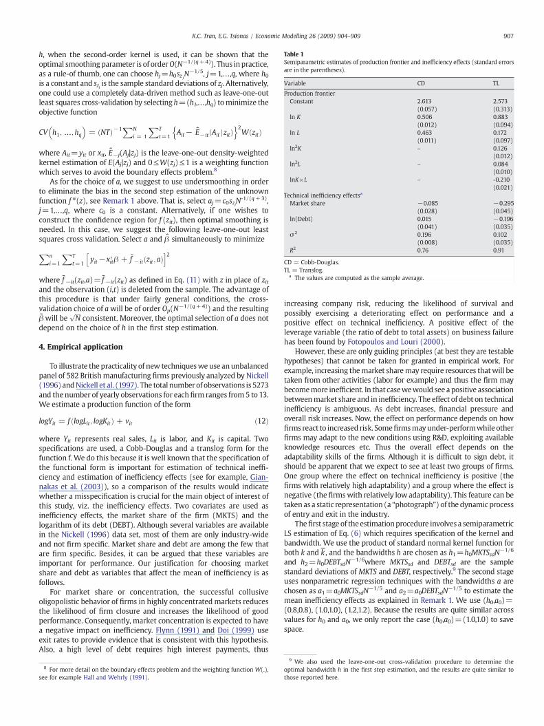
Table 1Semiparametric estimates of production frontier and inefficiency effects (standard errorsare in the parentheses).

Variable CD TL

Production frontierConstant 2.613 2.573

(0.057) (0.313)ln K 0.506 0.883

(0.012) (0.094)ln L 0.463 0.172

(0.011) (0.097)ln2K – 0.126

(0.012)ln2L – 0.084

(0.010)lnK×L – -0.210

(0.021)Technical inefficiency effectsa

Market share −0.085 −0.295(0.028) (0.045)

ln(Debt) 0.015 −0.196(0.041) (0.035)

σ 2 0.196 0.102(0.008) (0.035)

R2 0.76 0.91

CD = Cobb-Douglas.TL = Translog.

a The values are computed as the sample average.

907K.C. Tran, E.G. Tsionas / Economic Modelling 26 (2009) 904–909

h, when the second-order kernel is used, it can be shown that theoptimal smoothingparameter is of orderO(N−1/(q+4)). Thus inpractice,as a rule-of thumb, one can choose hj=h0sz j

N−1/5, j=1,…,q, where h0is a constant and szj is the sample standard deviations of zj. Alternatively,one could use a completely data-driven method such as leave-one-outleast squares cross-validation by selecting h=(h1,…,hq) tominimize theobjective function

CV h1; …;hq� �

= NTð Þ−1XNi = 1

XTt=1

Ait− E− it Ait jzitð Þn o2

W zitð Þ

where Ait=yit or xit, E−j(Aj|zj) is the leave-one-out density-weightedkernel estimation of E(Aj|zj) and 0≤W(zj)≤1 is a weighting functionwhich serves to avoid the boundary effects problem.8

As for the choice of a, we suggest to use undersmoothing in orderto eliminate the bias in the second step estimation of the unknownfunction f ⁎(z), see Remark 1 above. That is, select aj=c0szjN

-1/(q+3),j=1,…,q, where c0 is a constant. Alternatively, if one wishes toconstruct the confidence region for f (zit), then optimal smoothing isneeded. In this case, we suggest the following leave-one-out leastsquares cross validation. Select a and β simultaneously to minimize

Xni=1

XTt=1

yit−xit′ β + f − it zit ; að Þh i2

where f −it(zit,a)= f −it(zit) as defined in Eq. (11) with z in place of zitand the observation (i,t) is deleted from the sample. The advantage ofthis procedure is that under fairly general conditions, the cross-validation choice of awill be of order Op(N−1/(q+4)) and the resultingβwill be

ffiffiffiffiN

pconsistent. Moreover, the optimal selection of a does not

depend on the choice of h in the first step estimation.

4. Empirical application

To illustrate the practicality of new techniquesweuse an unbalancedpanel of 582 Britishmanufacturing firms previously analyzed by Nickell(1996) andNickell et al. (1997). The total numberof observations is 5273and the number of yearly observations for eachfirm ranges from 5 to 13.We estimate a production function of the form

logYit = f logLit ; logKitð Þ + vit ð12Þ

where Yit represents real sales, Lit is labor, and Kit is capital. Twospecifications are used, a Cobb-Douglas and a translog form for thefunction f. We do this because it is well known that the specification ofthe functional form is important for estimation of technical ineffi-ciency and estimation of inefficiency effects (see for example, Gian-nakas et al. (2003)), so a comparison of the results would indicatewhether a misspecification is crucial for the main object of interest ofthis study, viz. the inefficiency effects. Two covariates are used asinefficiency effects, the market share of the firm (MKTS) and thelogarithm of its debt (DEBT). Although several variables are availablein the Nickell (1996) data set, most of them are only industry-wideand not firm specific. Market share and debt are among the few thatare firm specific. Besides, it can be argued that these variables areimportant for performance. Our justification for choosing marketshare and debt as variables that affect the mean of inefficiency is asfollows.

For market share or concentration, the successful collusiveoligopolistic behavior of firms in highly concentrated markets reducesthe likelihood of firm closure and increases the likelihood of goodperformance. Consequently, market concentration is expected to havea negative impact on inefficiency. Flynn (1991) and Doi (1999) useexit rates to provide evidence that is consistent with this hypothesis.Also, a high level of debt requires high interest payments, thus

8 For more detail on the boundary effects problem and the weighting function W(.),see for example Hall and Wehrly (1991).

increasing company risk, reducing the likelihood of survival andpossibly exercising a deteriorating effect on performance and apositive effect on technical inefficiency. A positive effect of theleverage variable (the ratio of debt to total assets) on business failurehas been found by Fotopoulos and Louri (2000).

However, these are only guiding principles (at best they are testablehypotheses) that cannot be taken for granted in empirical work. Forexample, increasing themarket sharemay require resources thatwill betaken from other activities (labor for example) and thus the firm maybecomemore inefficient. In that casewewould see a positive associationbetweenmarket share and in inefficiency. The effect of debt on technicalinefficiency is ambiguous. As debt increases, financial pressure andoverall risk increases. Now, the effect on performance depends on howfirms react to increased risk. Somefirmsmayunder-performwhile otherfirms may adapt to the new conditions using R&D, exploiting availableknowledge resources etc. Thus the overall effect depends on theadaptability skills of the firms. Although it is difficult to sign debt, itshould be apparent that we expect to see at least two groups of firms.One group where the effect on technical inefficiency is positive (thefirms with relatively high adaptability) and a group where the effect isnegative (the firmswith relatively low adaptability). This feature can betaken as a static representation (a “photograph”) of the dynamic processof entry and exit in the industry.

Thefirst stage of theestimationprocedure involves a semiparametricLS estimation of Eq. (6) which requires specification of the kernel andbandwidth. We use the product of standard normal kernel function forboth k and k

–-, and the bandwidths h are chosen as h1=h0MKTSsdN

−1/6

and h2=h0DEBTsdN−1/6where MKTSsd and DEBTsd are the sample

standard deviations of MKTS and DEBT, respectively.9 The second stageuses nonparametric regression techniques with the bandwidths a arechosen as a1=a0MKTSsdN

−1/5 and a2=a0DEBTsdN−1/5 to estimate the

mean inefficiency effects as explained in Remark 1. We use (h0,a0)=(0.8,0.8), (1.0,1.0), (1.2,1.2). Because the results are quite similar acrossvalues for h0 and a0, we only report the case (h0,a0)=(1.0,1.0) to savespace.

9 We also used the leave-one-out cross-validation procedure to determine theoptimal bandwidth h in the first step estimation, and the results are quite similar tothose reported here.

10 For convenience we have converted technical inefficiency mean to technicalefficiency mean.

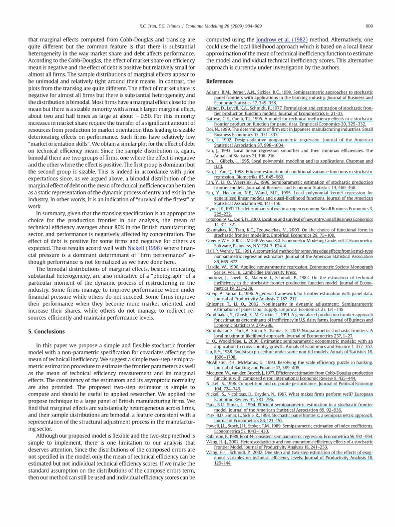
Fig. 1. Mean of technical efficiency.

Fig. 2. Marginal effects.

908 K.C. Tran, E.G. Tsionas / Economic Modelling 26 (2009) 904–909

4.1. Step1: Estimating the frontier parameters, β

The first step result, estimating the frontier parameters, β usingEq. (6) captures the marginal effects of capital and labour on output.The top panel of Table 1 reveals that the coefficients on the labour andcapital (production elasticities) have correct signs and are statisticallysignificant for both specifications of the frontier. Furthermore, thecoefficients on the second-order translog frontier are highly signifi-cant indicating that the Cobb-Douglas specification may not beadequate for this particular data set. Estimation based on the translogspecification has a goodness of fit R2=0.91, while estimation based onthe Cobb-Douglas specification has R2=0.76; consequently, theseresults suggest that translog specification is an appropriate choice forthe frontier in this case.

4.2. Step 2: Estimating the nonparametric function, f (z), and its marginaleffects, ∇f(z)

Next let us examine the effect of market share and debt on themean of technical efficiency using the second step estimation given inEqs. (9)–(11). We use the sample average (NT)−1Σi=1

N Σt=1T ∇f(zit) as

an estimator for the mean values of ∇f(zit). The results are presentedin the bottom panel of Table 1. For the translog specification, onaverage, the effects of market share and debt on the mean of technical

efficiency are negative and significant. In contrast, using the Cobb-Douglas specification for the frontier, the effect of market share onaverage is negative and significant but the magnitude of the effect isabout four times smaller. The effect of debt is positive but insignificanton average. This may be the result of misspecification in the frontier.

Sample densities of themean of technical efficiencymeasures10 forboth Cobb-Douglas and translog frontier are provided in Fig. 1. Themean efficiency distributions are different, implying that functionalform of the frontier is highly important for the mean efficiencymeasurement. According to Cobb-Douglas estimates, the distributionof the mean efficiency is multi-modal indicating substantial hetero-geneity. The mean efficiency averages about 84% with the majority ofthe firms having the efficiency mean in the range of 70% to 99%, and along tail to the left indicating the presence of highly less efficient firmsafter accounting, of course, for debt and market power as explanatoryvariables of technical inefficiency. For the translog estimates, thedistribution of the efficiency mean is also multi-modal with theefficiency mean averages about 80% with majority of firms havingefficiency mean in the range of 60% to 99%.

Fig. 2 provides the density plots for the marginal effects of marketshare and debt on the mean of efficiency. The densities in Fig. 2 show

909K.C. Tran, E.G. Tsionas / Economic Modelling 26 (2009) 904–909

that marginal effects computed from Cobb-Douglas and translog arequite different but the common feature is that there is substantialheterogeneity in the way market share and debt affects performance.According to the Cobb-Douglas, the effect of market share on efficiencymean is negative and the effect of debt is positive but relatively small foralmost all firms. The sample distributions of marginal effects appear tobe unimodal and relatively tight around their means. In contrast, theplots from the translog are quite different. The effect of market share isnegative for almost all firms but there is substantial heterogeneity andthedistribution is bimodal.Mostfirmshave amarginal effect close to themean but there is a sizable minority with a much largermarginal effect,about two and half times as large at about −0.50. For this minorityincreases in market share require the transfer of a significant amount ofresources from production to market orientation thus leading to sizabledeteriorating effects on performance. Such firms have relatively low“market orientation skills”. We obtain a similar plot for the effect of debton technical efficiency mean. Since the sample distribution is, again,bimodal there are two groups of firms, one where the effect is negativeand theotherwhere the effect is positive. Thefirst group is dominantbutthe second group is sizable. This is indeed in accordance with priorexpectations since, as we argued above, a bimodal distribution of themarginal effect of debt on themeanof technical inefficiencycanbe takenas a static representation of the dynamic process of entry and exit in theindustry. In other words, it is an indication of “survival of the fittest” atwork.

In summary, given that the translog specification is an appropriatechoice for the production frontier in our analysis, the mean oftechnical efficiency averages about 80% in the British manufacturingsector, and performance is negatively affected by concentration. Theeffect of debt is positive for some firms and negative for others asexpected. These results accord well with Nickell (1996) where finan-cial pressure is a dominant determinant of “firm performance” al-though performance is not formalized as we have done here.

The bimodal distributions of marginal effects, besides indicatingsubstantial heterogeneity, are also indicative of a “photograph” of aparticular moment of the dynamic process of restructuring in theindustry. Some firms manage to improve performance when underfinancial pressure while others do not succeed. Some firms improvetheir performance when they become more market oriented, andincrease their shares, while others do not manage to redirect re-sources efficiently and maintain performance levels.

5. Conclusions

In this paper we propose a simple and flexible stochastic frontiermodel with a non-parametric specification for covariates affecting themean of technical inefficiency. We suggest a simple two-step semipara-metric estimation procedure to estimate the frontier parameters as wellas the mean of technical efficiency measurement and its marginaleffects. The consistency of the estimators and its asymptotic normalityare also provided. The proposed two-step estimator is simple tocompute and should be useful to applied researcher. We applied thepropose technique to a large panel of British manufacturing firms. Wefind that marginal effects are substantially heterogeneous across firms,and their sample distributions are bimodal, a feature consistent with arepresentation of the structural adjustment process in the manufactur-ing sector.

Although our proposedmodel is flexible and the two-stepmethod issimple to implement, there is one limitation to our analysis thatdeserves attention. Since the distributions of the composed errors arenot specified in the model, only the mean of technical efficiency can beestimated but not individual technical efficiency scores. If we make thestandard assumption on the distributions of the compose errors term,then ourmethod can still be used and individual efficiency scores can be

computed using the Jondrow et al. (1982) method. Alternatively, onecould use the local likelihood approach which is based on a local linearapproximationof themeanof technical inefficiency function to estimatethe model and individual technical inefficiency scores. This alternativeapproach is currently under investigation by the authors.

References

Adams, R.M., Berger, A.N., Sickles, R.C., 1999. Semiparametric approaches to stochasticpanel frontiers with applications in the banking industry. Journal of Business andEconomic Statistics 17, 349–358.

Aigner, D., Lovell, K.A., Schmidt, P., 1977. Formulation and estimation of stochastic fron-tier production function models. Journal of Econometrics 6, 21–37.

Battese, G.E., Coelli, T.J., 1995. A model for technical inefficiency effects in a stochasticfrontier production function for panel data. Empirical Economics 20, 325–332.

Doi, N., 1999. The determinants of firm exit in Japanese manufacturing industries. SmallBusiness Economics 13, 331–337.

Fan, J., 1992. Design-adaptive nonparametric regression. Journal of the AmericanStatistical Association 87, 998–1004.

Fan, J., 1993. Local linear regression smoother and their minimax efficiencies. TheAnnals of Statistics 21, 196–216.

Fan, J., Gijbels, I., 1995. Local polynomial modeling and its applications. Chapman andHall.

Fan, J., Yao, Q., 1998. Efficient estimation of conditional variance functions in stochasticregression. Biometrika 85, 645–660.

Fan, Y., Li, Q., Weersink, A., 1996. Semiparametric estimation of stochastic productionfrontier models. Journal of Business and Economic Statistics 14, 460–468.

Fan, Y., Heckman, N.E., Wand, M.P., 1995. Local polynomial kernel regression forgeneralized linear models and quasi-likelihood functions. Journal of the AmericanStatistical Association 90, 141–150.

Flynn, J.E.,1991. The determinants of exit in an open economy. Small Business Economics 3,225–232.

Fotopoulos, G., Louri, H., 2000. Location and survival of newentry. Small Business Economics14, 311–321.

Giannakas, K., Tran, K.C., Tzouvelekas, V., 2003. On the choice of functional form instochastic frontier modeling. Empirical Economics 28, 75–100.

Greene,W.H., 2002. LIMDEP, Version8.0: EconometricModelingGuide, vol. 2. EconometricSoftware, Plainview, N.Y. E24-3–E24-4.

Hall, P.,Wehrly, T.E.,1991. A geometricalmethod for removing edge effects fromkernel-typenonparametric regression estimators. Journal of the American Statistical Association86, 665–672.

Hardle, W., 1990. Applied nonparametric regression. Econometric Society MonographSeries, vol. 19. Cambridge University Press.

Jondrow, J., Lovell, K., Materov, I., Schmidt, P., 1982. On the estimation of technicalinefficiency in the stochastic frontier production function model. Journal of Econo-metrics 19, 233–238.

Kneip, A., Simar, L., 1996. A general framework for frontier estimation with panel data.Journal of Productivity Analysis 7, 187–212.

Kniesner, T., Li, Q., 2002. Nonlinearity in dynamic adjustment: Semiparametricestimation of panel labor supply. Empirical Economics 27, 131–148.

Kumbhakar, S., Ghosh, S., McGuckin, T., 1991. A generalized production frontier approachfor estimating determinants of inefficiency in U.S. dairy farms. Journal of Business andEconomic Statistics 9, 279–286.

Kumbhakar, S., Park, A., Simar, S., Tsionas, E., 2007. Nonparametric stochastic frontiers: Alocal maximum likelihood approach. Journal of Econometrics 237, 1–27.

Li, Q., Wooldridge, J., 2000. Estimating semiparametric econometric models: with anapplication to cross-country growth. Annals of Economics and Finance 1, 337–357.

Liu, R.Y., 1988. Bootstrap procedure under some non-iid models. Annals of Statistics 16,1696–1708.

McAllister, P.H., McManus, D., 1993. Resolving the scale efficiency puzzle in banking.Journal of Banking and Finance 17, 389–405.

Meeusen,W., vanden Broeck, J.,1977. Efficiencyestimation fromCobb-Douglas productionfunctions with composed error. International Economic Review 8, 435–444.

Nickell, S., 1996. Competition and corporate performance. Journal of Political Economy104, 724–746.

Nickell, S., Nicolitsas, D., Dryden, N., 1997. What makes firms perform well? EuropeanEconomic Review 41, 783–796.

Park, B.U., Simar, L., 1994. Efficient semiparametric estimation in a stochastic frontiermodel. Journal of the American Statistical Association 89, 92–936.

Park, B.U., Simar, L., Sickle, R.,1998. Stochastic panel frontiers: a semiparametric approach.Journal of Econometrics 84, 121–152.

Powell, J.L., Stock, J.H., Stoker, T.M., 1989. Semiparametric estimation of index coefficients.Econometrica 57, 1043–1430.

Robinson, P.,1988. Root-N-consistent semiparametric regression. Econometrica 56, 931–954.Wang, H.-J., 2002. Heteroscedasticity and non-monotonic efficiency effects of a stochastic

Frontier Model. Journal of Productivity Analysis 18, 241–253.Wang, H.-J., Schmidt, P., 2002. One-step and two-step estimation of the effects of exog-

enous variables on technical efficiency levels. Journal of Productivity Analysis 18,129–144.