Nonmonotonic Logic and Rule-Based Legal Reasoning

UC IrvineUC Irvine Electronic Theses and Dissertations

TitleNonmonotonic Logic and Rule-Based Legal Reasoning

Permalinkhttps://escholarship.org/uc/item/59j2j45w

AuthorLawsky, Sarah

Publication Date2017 Peer reviewed|Thesis/dissertation

eScholarship.org Powered by the California Digital LibraryUniversity of California

UNIVERSITY OF CALIFORNIA,IRVINE

Nonmonotonic Logic and Rule-Based Legal Reasoning

DISSERTATION

submitted in partial satisfaction of the requirementsfor the degree of

DOCTOR OF PHILOSOPHY

in Philosophy

by

Sarah Beth Lawsky

Dissertation Committee:Professor Kai Wehmeier, Chair

Assistant Professor Jeffrey HelmreichAssociate Professor Sean Walsh

2017

A version of Chapter 2 is forthcoming in and c© the Florida Tax ReviewAll other materials c© 2017 Sarah Beth Lawsky

DEDICATION

For my mother, Ellen Lawsky.

ii

TABLE OF CONTENTS

Page

LIST OF FIGURES vi

LIST OF TABLES vii

ACKNOWLEDGMENTS viii

CURRICULUM VITAE ix

ABSTRACT OF THE DISSERTATION x

1 Definitional scope in the Internal Revenue Code 11.1 Introduction . . . . . . . . . . . . . . . . . . . . . . . . . . . . . . . . . . . . . 11.2 The problem of definitional scope . . . . . . . . . . . . . . . . . . . . . . . . . 4

1.2.1 Home mortgage interest deduction . . . . . . . . . . . . . . . . . . . 61.2.2 Substantially disproportionate corporate distribution . . . . . . . . . 111.2.3 Resolving problems of definitional scope . . . . . . . . . . . . . . . . 19

1.3 A general solution: formalizing the Code . . . . . . . . . . . . . . . . . . . . 221.4 Formalizations . . . . . . . . . . . . . . . . . . . . . . . . . . . . . . . . . . . . 26

1.4.1 Home mortgage interest deduction . . . . . . . . . . . . . . . . . . . 261.4.2 Disproportionate distribution . . . . . . . . . . . . . . . . . . . . . . . 29

1.5 Conclusion . . . . . . . . . . . . . . . . . . . . . . . . . . . . . . . . . . . . . . 32

2 Modeling rule-based legal reasoning 332.1 Introduction . . . . . . . . . . . . . . . . . . . . . . . . . . . . . . . . . . . . . 332.2 Defeasible reasoning and default logic . . . . . . . . . . . . . . . . . . . . . . 352.3 Formalizing Section 163 . . . . . . . . . . . . . . . . . . . . . . . . . . . . . . 402.4 The benefits of nonmonotonicity . . . . . . . . . . . . . . . . . . . . . . . . . 442.5 Conclusion: The benefits of default logic . . . . . . . . . . . . . . . . . . . . . 50

2.5.1 Theory . . . . . . . . . . . . . . . . . . . . . . . . . . . . . . . . . . . . 512.5.2 Practice . . . . . . . . . . . . . . . . . . . . . . . . . . . . . . . . . . . . 53

3 What default rules are not 553.1 Introduction . . . . . . . . . . . . . . . . . . . . . . . . . . . . . . . . . . . . . 553.2 Horty’s approach . . . . . . . . . . . . . . . . . . . . . . . . . . . . . . . . . . 56

3.2.1 Horty on default logic . . . . . . . . . . . . . . . . . . . . . . . . . . . 56

iii

3.2.2 Horty on deontic reasoning . . . . . . . . . . . . . . . . . . . . . . . . 603.3 Probability and fixed-priority default theories . . . . . . . . . . . . . . . . . . 62

3.3.1 The Cuba example . . . . . . . . . . . . . . . . . . . . . . . . . . . . . 623.3.2 Probabilities . . . . . . . . . . . . . . . . . . . . . . . . . . . . . . . . . 64

3.4 Specificity . . . . . . . . . . . . . . . . . . . . . . . . . . . . . . . . . . . . . . 673.4.1 The skeptical inheritance networks approach . . . . . . . . . . . . . . 673.4.2 The technical claim: Order of application . . . . . . . . . . . . . . . . 743.4.3 The intuitive claim: What is specificity? . . . . . . . . . . . . . . . . . 77

3.5 Generics . . . . . . . . . . . . . . . . . . . . . . . . . . . . . . . . . . . . . . . 853.5.1 What are generics? . . . . . . . . . . . . . . . . . . . . . . . . . . . . . 863.5.2 Some generics are not default rules . . . . . . . . . . . . . . . . . . . . 893.5.3 Some default rules are not generics . . . . . . . . . . . . . . . . . . . . 90

3.6 Conclusion: Legal rules as default rules . . . . . . . . . . . . . . . . . . . . . 91

4 Statutes as supernormal rules 934.1 Introduction . . . . . . . . . . . . . . . . . . . . . . . . . . . . . . . . . . . . . 934.2 Interpreting statutory rules . . . . . . . . . . . . . . . . . . . . . . . . . . . . 944.3 Horty’s puzzles . . . . . . . . . . . . . . . . . . . . . . . . . . . . . . . . . . . 96

4.3.1 The Order Puzzle . . . . . . . . . . . . . . . . . . . . . . . . . . . . . . 964.3.2 Inappropriate equilibria . . . . . . . . . . . . . . . . . . . . . . . . . . 101

4.4 Possible objections . . . . . . . . . . . . . . . . . . . . . . . . . . . . . . . . . 1024.4.1 Does defeasibility remain? . . . . . . . . . . . . . . . . . . . . . . . . . 1024.4.2 Statutory rules with premises . . . . . . . . . . . . . . . . . . . . . . . 1034.4.3 A simpler approach: order of application . . . . . . . . . . . . . . . . 1044.4.4 Embedded oughts . . . . . . . . . . . . . . . . . . . . . . . . . . . . . 1044.4.5 Conditional commands . . . . . . . . . . . . . . . . . . . . . . . . . . 104

4.5 Conclusion . . . . . . . . . . . . . . . . . . . . . . . . . . . . . . . . . . . . . . 106

Bibliography 109

References 109

Appendix A Statutory language 113

Appendix B Justifying stable scenarios 117B.1 The Cuba Example . . . . . . . . . . . . . . . . . . . . . . . . . . . . . . . . . 118

B.1.1 The theories . . . . . . . . . . . . . . . . . . . . . . . . . . . . . . . . . 118B.1.2 The rules . . . . . . . . . . . . . . . . . . . . . . . . . . . . . . . . . . . 119B.1.3 Analysis . . . . . . . . . . . . . . . . . . . . . . . . . . . . . . . . . . . 124

B.2 The Order Puzzle . . . . . . . . . . . . . . . . . . . . . . . . . . . . . . . . . . 124B.2.1 The theories . . . . . . . . . . . . . . . . . . . . . . . . . . . . . . . . . 124B.2.2 The rules . . . . . . . . . . . . . . . . . . . . . . . . . . . . . . . . . . . 125B.2.3 Analysis . . . . . . . . . . . . . . . . . . . . . . . . . . . . . . . . . . . 129

B.3 Supernormal Order Puzzle . . . . . . . . . . . . . . . . . . . . . . . . . . . . . 130B.3.1 The theories . . . . . . . . . . . . . . . . . . . . . . . . . . . . . . . . . 130

iv

B.3.2 The rules . . . . . . . . . . . . . . . . . . . . . . . . . . . . . . . . . . . 131B.3.3 Analysis . . . . . . . . . . . . . . . . . . . . . . . . . . . . . . . . . . . 137

B.4 Inappropriate equilibrium . . . . . . . . . . . . . . . . . . . . . . . . . . . . . 137B.4.1 The theory . . . . . . . . . . . . . . . . . . . . . . . . . . . . . . . . . . 137B.4.2 The rules . . . . . . . . . . . . . . . . . . . . . . . . . . . . . . . . . . . 138B.4.3 Analysis . . . . . . . . . . . . . . . . . . . . . . . . . . . . . . . . . . . 142

B.5 Supernormal inappropriate equilibrium . . . . . . . . . . . . . . . . . . . . . 143B.5.1 The theory . . . . . . . . . . . . . . . . . . . . . . . . . . . . . . . . . . 143B.5.2 The rules . . . . . . . . . . . . . . . . . . . . . . . . . . . . . . . . . . . 143B.5.3 Analysis . . . . . . . . . . . . . . . . . . . . . . . . . . . . . . . . . . . 146

v

LIST OF FIGURES

Page

1.1 Correct Analysis . . . . . . . . . . . . . . . . . . . . . . . . . . . . . . . . . . . 161.2 Incorrect Analysis . . . . . . . . . . . . . . . . . . . . . . . . . . . . . . . . . . 171.3 Legislative History . . . . . . . . . . . . . . . . . . . . . . . . . . . . . . . . . 18

3.1 The Cuba example . . . . . . . . . . . . . . . . . . . . . . . . . . . . . . . . . 633.2 Base Rates: Cuban Resident, U.S. Citizen (not to scale) . . . . . . . . . . . . . 663.3 The Cuba example, problematized . . . . . . . . . . . . . . . . . . . . . . . . 673.4 The Nixon diamond . . . . . . . . . . . . . . . . . . . . . . . . . . . . . . . . 693.5 The modified Cuba example . . . . . . . . . . . . . . . . . . . . . . . . . . . . 753.6 The Tweety example . . . . . . . . . . . . . . . . . . . . . . . . . . . . . . . . 823.7 Groups . . . . . . . . . . . . . . . . . . . . . . . . . . . . . . . . . . . . . . . . 84

vi

LIST OF TABLES

Page

3.1 Tweety 1 . . . . . . . . . . . . . . . . . . . . . . . . . . . . . . . . . . . . . . . 613.2 Tweety 2 . . . . . . . . . . . . . . . . . . . . . . . . . . . . . . . . . . . . . . . 623.3 Probability example: groups . . . . . . . . . . . . . . . . . . . . . . . . . . . . 83

B.1 The Cuba example . . . . . . . . . . . . . . . . . . . . . . . . . . . . . . . . . 124B.2 The Order Puzzle . . . . . . . . . . . . . . . . . . . . . . . . . . . . . . . . . . 129B.3 The supernormal Order Puzzle . . . . . . . . . . . . . . . . . . . . . . . . . . 137B.4 Inappropriate equilibrium . . . . . . . . . . . . . . . . . . . . . . . . . . . . . 142B.5 Supernormal inappropriate equilibrium . . . . . . . . . . . . . . . . . . . . . 146

vii

ACKNOWLEDGMENTS

Thanks to the following.

Those who read and commented on various drafts of various chapters, especially theparticipants in the UC Irvine Logic Colloquium from 2013 to 2016.

Kai Wehmeier, Sean Walsh, Jeffrey Helmreich.

Patty Jones, John Sommerhauser; Brian Rogers; Kyle Banick, J. Ethan Galebach, J.R. Schatz;Jeremy Heis, Simon Huttegger, Richard Mendelsohn, Cailin O’Connor, J. Kyle Stanford,Jim Weatherall; Barbara Sarnecka.

The faculty and students of UCI LPS, the most challenging, intimidating, friendly, provoca-tive place I have done academic work as either a student or faculty member.

David Malament and Erwin Chemerinsky, each of whose various interventions made thisdegree possible for me.

Jeff Horty, Marek Sergot.

Joshua Blank, Neil Buchanan, Elizabeth Emens, Ruth Mason.

Joshua Kleinfeld, Daniel Rodriguez.

Leslie, Maggie.

Lawskys: Amy, Henry, and Mattea (and Herman); David and Ellen; Matthew.

And finally, particular thanks to my mother, Ellen Lawsky. She showed me that a womanwith two small children can study for a Ph.D. (statistics, in her case), and she has steadilysupported and encouraged my interest in math and logic, including letting me adopt hercopy of Irving Copi’s Symbolic Logic when I was in sixth grade. And when, as an adult, Icalled her to tell her I had finished my LL.M. in tax law, she said, “That’s nice. You’ll geta Ph.D. now.” It was not clear whether this was a prediction or a command, but at anyrate, Mom, as always, you were right. This dissertation is for you.

viii

CURRICULUM VITAE

Sarah Beth Lawsky

EDUCATION

Doctor of Philosophy in Philosophy 2017University of California, Irvine Irvine, California

Master of Laws in Taxation 2007New York University School of Law New York, New York

Juris Doctor 2001Yale Law School New Haven, Connecticut

Bachelor of Arts in Philosophy with an Allied Field of Math 1994University of Chicago Chicago, Illinois

ix

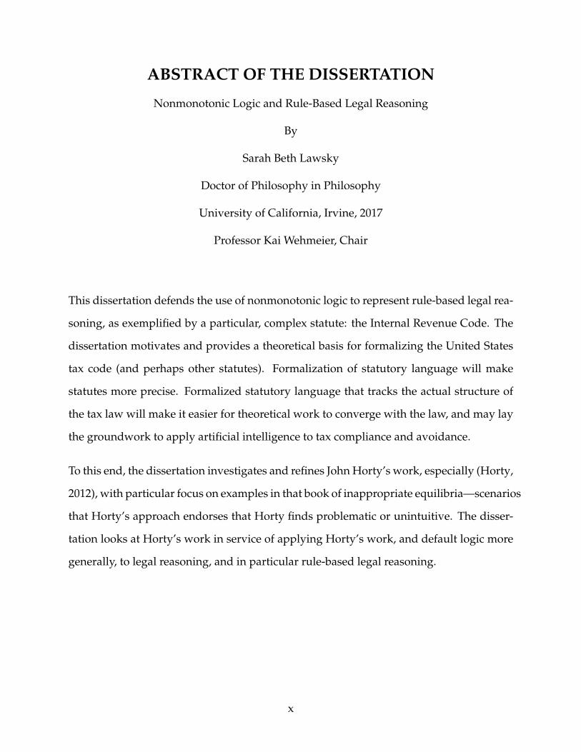
ABSTRACT OF THE DISSERTATION

Nonmonotonic Logic and Rule-Based Legal Reasoning

By

Sarah Beth Lawsky

Doctor of Philosophy in Philosophy

University of California, Irvine, 2017

Professor Kai Wehmeier, Chair

This dissertation defends the use of nonmonotonic logic to represent rule-based legal rea-

soning, as exemplified by a particular, complex statute: the Internal Revenue Code. The

dissertation motivates and provides a theoretical basis for formalizing the United States

tax code (and perhaps other statutes). Formalization of statutory language will make

statutes more precise. Formalized statutory language that tracks the actual structure of

the tax law will make it easier for theoretical work to converge with the law, and may lay

the groundwork to apply artificial intelligence to tax compliance and avoidance.

To this end, the dissertation investigates and refines John Horty’s work, especially (Horty,

2012), with particular focus on examples in that book of inappropriate equilibria—scenarios

that Horty’s approach endorses that Horty finds problematic or unintuitive. The disser-

tation looks at Horty’s work in service of applying Horty’s work, and default logic more

generally, to legal reasoning, and in particular rule-based legal reasoning.

x

Chapter 1

Definitional scope in the Internal

Revenue Code

1.1 Introduction

The Internal Revenue Code is notoriously complex. Sometimes its complexity is at-

tributed to its size, or to its graduated rate schedule, or to the many exceptions to general

rules that permeate the statute. But part of its complexity is due to its structure, which in

turn is due in part to the Code’s many interlinked sections, to the “dependencies” among

the various sections of the Code (Katz & Ruhl, 2015). This chapter identifies and analyzes

a particular type of dependency in the Code, what it terms the problem of “definitional

scope,” and uses the problem of definitional scope as a case study to argue for the benefit

of formalizing proposed legislation.

The Internal Revenue Code is rife with explicit cross-references, and almost all of those are

internal cross-references—references within the Internal Revenue Code to other sections

of the Internal Revenue Code. Approximately 97% of citations in the Internal Revenue

1

Code are to sections within the Code, rendering the Code “almost entirely self-contained”

(Katz & Bommarito II, 2014). For example:

No gain or loss shall be recognized if property is transferred to a corporation

by one or more persons solely in exchange for stock in such corporation and

immediately after the exchange such person or persons are in control (as de-

fined in section 368(c)) of the corporation.

(Internal Revenue Code, Section 351(a)) (emphasis added)

This statute, Section 351(a), explicitly calls Section 368(c). But other dependencies arise

not from explicit cross-reference, but from definitions. Definitions, like explicit cross-

reference, call other portions of the Code, but they do so implicitly. Thus, for example:

This paragraph shall not apply to any redemption made pursuant to a plan the

purpose of effect of which is a series of redemptions resulting in a distribution

which (in the aggregate) is not substantially disproportionate with respect to the

shareholder.

(Internal Revenue Code, Section 302(b)(2)(D)) (emphasis added)

The phrase “substantially disproportionate” in Section 302 is defined earlier in the same

section, and thus calls earlier language.

Cross-references and definitions need not be distinct—a Code section can cross-reference

a definition, as in “property (as defined in [S]ection 317(a)),” which appears in Section

301. But a definition need not be explicitly cross-referenced to apply. It is these non-

explicitly cross-referenced definitions that this chapter studies. In particular, the chapter

studies examples of problems of definitional scope: when the Code uses a term but the

structure of the Code leaves unclear to what a term refers.

2

The chapter studies such definitions in service of two larger points. First, the chapter

draws attention to a different sort of ambiguity than that usually studied in the Internal

Revenue Code. There are any number of projects studying ambiguity of the meaning of

terms or phrases in the Code in particular (e.g., (Geier, 1994), (Heen, 1996), (McCaffery,

1996), (McCormack, 2009)) and in statutes and other sources of law in general

(e.g., (Alexander & Sherwin, 2008, Part III). But little attention is paid to ambiguity in the

structure of the Code.1 I do not mean “structure” in the sense that it is sometimes defined:

as “the theoretical construct that overarches the sum total of the entire Internal Revenue

Code. . . [and] includes such ideas as the same dollars should not be taxed to the same

person more than once” (Geier, 1994, p. 497). Rather, I mean structure in the sense of the

formal interrelation of the parts of the Code.

To understand the structure of a statute and resolve its ambiguities, one must understand

the substance of that statute. But the structure itself is in some sense the skeleton on

which the substance is hung (though the two can never really be separated). The structure

of the Code has at least three components: rule interaction, scope, and cross-reference.

This chapter deals with a portion of the last component, as definition is a type of cross-

reference.

Second, the chapter uses the example of definitional scope as a case study to encourage

formalization of proposed legislation. Formalization would have a range of advantages.

It could help drafters avoid unintentional ambiguity and refine the language used in the

statute; it could provide helpful guidance for those wishing to interpret the statute; and

it could help move the law closer to legibility by a computer—that is, it could help on

the journey to actual legal artificial intelligence. This chapter thus builds upon the work

of Layman Allen, though it also differs from that work. Most significantly, while Allen

1An important exception this is the work of Layman Allen, e.g., (L. E. Allen, 1956), (L. Allen, 1980), andespecially (L. E. Allen & Engholm, 1979), which describes four types of ambiguity that can arise from im-precise drafting. He differentiates between ambiguity within sentences and among sentences; “definitionalscope,” as I describe it in this chapter, could be any of Allen’s four types of ambiguity.

3

argues that formal logic should be included in statutes, this chapter encourages a more

moderate approach, in which drafters would use formalization of language as a tool to

guide them in drafting, but the legislation itself would remain free of formalization.

1.2 The problem of definitional scope

An explicit definition in the Internal Revenue Code, like definitions in statutes in gen-

eral, provides a set of words that can be substituted throughout the text for another word

or set of words. Definitions in the Code are extensional: if X = Y, then anywhere in

the Code that X appears, Y can be substituted salva veritate. Such definitions may seem

simple: as one scholar has written, “when Congress inserts a definitional section, courts

resort. . . to the statutory definition alone. Congress in effect replaces a fuzzy and com-

plicated algorithm with a simple cut-and-paste function: ‘Where one sees X, one shall

read Y”’ (Rosenkranz, 2002, p. 2104). For example, the U.S. Code defines “person” as

including “corporations, companies, associations, firms, partnerships, societies, and joint

stock companies, as well as individuals.” Thus wherever one sees the term “person”

(“Every United States person shall furnish. . . such information as the Secretary may pre-

scribe. . . .”), one substitutes “corporations, companies” and so forth.

But in fact, what this putatively simple cut-and-paste function requires can itself be am-

biguous and require further inquiry of the sort one usually associates with statutory in-

terpretation. The complication comes not in the “cut and paste” portion, but rather in

deciding what one should highlight, as it were, to cut and paste.

As this section describes more fully, some sections of the Code involve a problem of the

following form:

Main Rule: If A is X, then B.

4

Definition: X means [definition].

Limitation: This section applies only if A has characteristic Y.

Other Rule: If A is X, then C.

The question is what to do when A is X, but A does not have characteristic Y. Does

C hold? Is the definition of X contained only in the definition section? Or should the

limitation be incorporated into the definition?

It may seem obvious from the abstraction that if A is X, then C, regardless of whether A

has characteristic Y. It’s true that the main rule applies only if A has characteristic Y. But

why should that carry over to the Other Rule? After all, aren’t definitions are a “simple

cut-and-paste function”? In fact, as an examination of the actual law in this area shows,

the answer is far from clear.

While ambiguity is not always problematic, unintentional ambiguity can create a range of

problems. Unclear law increases the compliance burden, as even taxpayers who want to

comply must spend time and money attempting to determine what the law means. Com-

plexity can also be dispiriting to taxpayers and thus reduce voluntary compliance (Joint

Committee on Taxation, 1998, p. 142). Ambiguity in the law also creates burdens for the

IRS, which must help taxpayers comply. Moreover, because an ambiguous provision has

at least two reasonable interpretations, ambiguous provisions can lead to increased au-

dits, more protracted audits, and even litigation, all of which creates additional burdens

for both taxpayers and the government. Congress itself recognizes the problem of unin-

tentional ambiguity in the law; it has mandated an annual Tax Law Complexity Analysis,

which is to include, inter alia, areas “in which the law is uncertain” (Internal Revenue

Service Restructuring and Reform Act of 1998, 1998, Section 4022(a)). Unintentionally

ambiguous definitional scope, which this section describes, is thus a problem.

This section looks at the problem as it arises in the context of, first, the home mortgage

5

interest deduction, and, second, corporate redemptions. Because the statutory text is crit-

ical for this analysis, the relevant portions of the statutes described below are reproduced

in Appendix A.

1.2.1 Home mortgage interest deduction

The problem of definitional scope appears in Section 163(h) of the Internal Revenue Code,

which addresses the home mortgage interest deduction. This section first describes the

relevant law and then highlights the structural ambiguity.

In general, interest payments are deductible (Section 163(a))2. However, personal interest

payments are not deductible (Section 163(h)(1)). “Personal interest payments” are de-

fined by exclusion: all payments are personal interest payments except six discrete items,

including “qualified residence interest,” commonly known as “home mortgage interest”

(Section 163(h)(2)(D)).

The statute defines qualified residence interest as interest accrued on either “acquisition

indebtedness” or “home equity indebtedness,” both with regard to a “qualified resi-

dence” of the taxpayer, up to a certain amount of indebtedness (Section 163(h)(3)(A)).

A “qualified residence” includes both the taxpayer’s principal residence and any other

residence of the taxpayer if the taxpayer makes an election to count that residence as a

qualified residence (163(h)(4)(A)).

Acquisition indebtedness is defined in Section 163(h)(B)(i) as debt that “is incurred in

acquiring, constructing, or substantially improving a qualified residence of the taxpayer,

and . . . that is secured by such residence” (Section 163(h)(3)(B)(i)) Under a separate

“Limitation” provision in Section 163(h)(B)(ii), the maximum amount that can be “treated

2Parenthetical references are to sections of the Internal Revenue Code or the regulations thereunder.

6

as” acquisition indebtedness for a given year is $1 million.

For example, imagine a taxpayer who purchases a $1.4 million primary residence with

$300,000 cash and takes out a $1.1 million purchase money mortgage that is secured by

the house. The interest rate on the debt is 8%, accruing and payable annually, so the

taxpayer owes $88,000 of interest per year. However, not all of the $88,000 is deductible

under the acquisition indebtedness provision, because only the interest on $1 million is

deductible with respect to acquisition indebtedness, and the $88,000 represents interest

on $1.1 million. With respect to acquisition indebtedness, the taxpayer may deduct only

the proportionate amount of interest—the number that stands in the same proportion to

$88,000 that $1 million bears to $1.1 million. Therefore, the taxpayer may deduct $80,000

as interest on acquisition indebtedness.

However, the statute also allows a deduction for another type of home mortgage inter-

est, interest on home equity indebtedness. Home equity indebtedness is debt that is not

acquisition indebtedness and that is secured by a qualified residence, subject to two re-

strictions. First, debt is home equity indebtedness only to the extent that the debt does

not exceed the fair market value of the qualified residence reduced by the amount of ac-

quisition indebtedness with respect to that residence. Second, the total amount treated as

home equity indebtedness cannot exceed $100,000.

As another example, consider a taxpayer in the highest tax bracket who buys a home for

$600,000, all of which is paid for using debt secured by the house, and assume that she

uses the home as her principal residence. She pays 10% annual interest on the debt, all

of which is acquisition indebtedness. Each year, therefore, she may deduct $60,000 with

respect to the debt.

After a few years, she has paid down none of the principal on the first loan, and because

the value of her house has increased to $750,000, another lender is willing to lend her

7

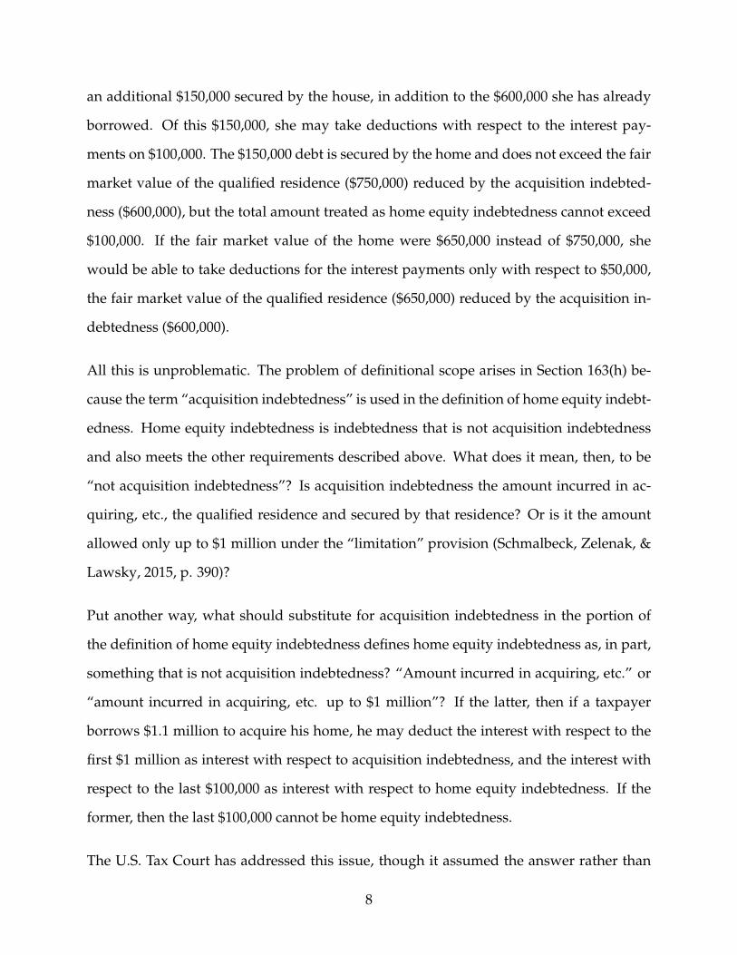
an additional $150,000 secured by the house, in addition to the $600,000 she has already

borrowed. Of this $150,000, she may take deductions with respect to the interest pay-

ments on $100,000. The $150,000 debt is secured by the home and does not exceed the fair

market value of the qualified residence ($750,000) reduced by the acquisition indebted-

ness ($600,000), but the total amount treated as home equity indebtedness cannot exceed

$100,000. If the fair market value of the home were $650,000 instead of $750,000, she

would be able to take deductions for the interest payments only with respect to $50,000,

the fair market value of the qualified residence ($650,000) reduced by the acquisition in-

debtedness ($600,000).

All this is unproblematic. The problem of definitional scope arises in Section 163(h) be-

cause the term “acquisition indebtedness” is used in the definition of home equity indebt-

edness. Home equity indebtedness is indebtedness that is not acquisition indebtedness

and also meets the other requirements described above. What does it mean, then, to be

“not acquisition indebtedness”? Is acquisition indebtedness the amount incurred in ac-

quiring, etc., the qualified residence and secured by that residence? Or is it the amount

allowed only up to $1 million under the “limitation” provision (Schmalbeck, Zelenak, &

Lawsky, 2015, p. 390)?

Put another way, what should substitute for acquisition indebtedness in the portion of

the definition of home equity indebtedness defines home equity indebtedness as, in part,

something that is not acquisition indebtedness? “Amount incurred in acquiring, etc.” or

“amount incurred in acquiring, etc. up to $1 million”? If the latter, then if a taxpayer

borrows $1.1 million to acquire his home, he may deduct the interest with respect to the

first $1 million as interest with respect to acquisition indebtedness, and the interest with

respect to the last $100,000 as interest with respect to home equity indebtedness. If the

former, then the last $100,000 cannot be home equity indebtedness.

The U.S. Tax Court has addressed this issue, though it assumed the answer rather than

8

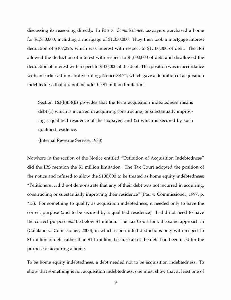
discussing its reasoning directly. In Pau v. Commissioner, taxpayers purchased a home

for $1,780,000, including a mortgage of $1,330,000. They then took a mortgage interest

deduction of $107,226, which was interest with respect to $1,100,000 of debt. The IRS

allowed the deduction of interest with respect to $1,000,000 of debt and disallowed the

deduction of interest with respect to $100,000 of the debt. This position was in accordance

with an earlier administrative ruling, Notice 88-74, which gave a definition of acquisition

indebtedness that did not include the $1 million limitation:

Section 163(h)(3)(B) provides that the term acquisition indebtedness means

debt (1) which is incurred in acquiring, constructing, or substantially improv-

ing a qualified residence of the taxpayer, and (2) which is secured by such

qualified residence.

(Internal Revenue Service, 1988)

Nowhere in the section of the Notice entitled “Definition of Acquisition Indebtedness”

did the IRS mention the $1 million limitation. The Tax Court adopted the position of

the notice and refused to allow the $100,000 to be treated as home equity indebtedness:

“Petitioners . . . did not demonstrate that any of their debt was not incurred in acquiring,

constructing or substantially improving their residence” (Pau v. Commissioner, 1997, p.

*13). For something to qualify as acquisition indebtedness, it needed only to have the

correct purpose (and to be secured by a qualified residence). It did not need to have

the correct purpose and be below $1 million. The Tax Court took the same approach in

(Catalano v. Comissioner, 2000), in which it permitted deductions only with respect to

$1 million of debt rather than $1.1 million, because all of the debt had been used for the

purpose of acquiring a home.

To be home equity indebtedness, a debt needed not to be acquisition indebtedness. To

show that something is not acquisition indebtedness, one must show that at least one of

9

the parts of its definition fails to hold. If the only two parts of the definition are a correct

purpose (buying a home) and the correct security (the home), then if both are true, the

debt in question is acquisition indebtedness and cannot be home equity indebtedness. But

if there is a third prong, the “less than $1 million” prong, and that prong fails to hold, the

whole definition fails, because the definition is conjunctive, and thus each part is required

in ordered for the debt to be acquisition indebtedness.

Interestingly, the IRS subsequently disavowed this win and issued a ruling that it would

not follow Pau and would permit interest deductions with respect to $1.1 million of debt

even if all of the debt was used for acquiring, constructing, or substantially improving a

residence. The ruling incorporated the $1 million limitation into the definition of “acqui-

sition indebtedness”:

Section 163(h)(3)(B)(i) provides that acquisition indebtedness is any indebted-

ness that is incurred in acquiring, constructing, or substantially improving a

qualified residence and is secured by the residence. However, 163(h)(3)(B)(ii)

limits the amount of indebtedness treated as acquisition indebtedness to $1,000,000

($500,000 for a married individual filing separately). Accordingly, any indebted-

ness described in Section 163(h)(3)(B)(i) in excess of $1,000,000 is, by definition, not

acquisition indebtedness for purposes of Section 163(h)(3).

(Internal Revenue Service, 2010) (emphasis added)

This stands in contrast to its definition of acquisition indebtedness in the earlier IRS no-

tice. The Tax Court subsequently adopted this position as well (Edosada v. Comissioner,

2012). The problem of definitional scope in Section 163(h) was thus finally recognized

and resolved by the IRS and Tax Court.

10

1.2.2 Substantially disproportionate corporate distribution

A similar ambiguity arises in the context of corporate redemptions. There are two possible

tax characterizations when a corporation acquires its own stock from its shareholder in

exchange for money or other property. Because such a transaction resembles both a sale

by the shareholder and a distribution of corporate assets, the redemption may be treated

as a sale or exchange of the stock, on the one hand, or as a distribution to the shareholder,

on the other (Section 302).

The distinction matters to taxpayers for two possible reasons. First, for either corporate

or individual taxpayers, a “sale or exchange” transaction lets the taxpayer recover basis,

generally lowering the amount of income subject to tax (Section 1001). Second, corporate

shareholders pay little or no tax on dividends received from other corporations due to the

dividends-received deduction (Section 243). (Under current law, most dividends received

by individuals are taxed at capital gains rates, so whether the distribution is taxed as a

dividend or a sale or exchange does not affect the rate at which taxed is imposed on

individuals (Section 1(h)(11)). Section 302 determines which treatment properly applies

in which circumstances.

Consider, for example, the situation in which a corporation has one shareholder who

owns all of the corporate stock. If the corporation redeems some portion of that share-

holder’s shares in exchange for money, the shareholder still owns all of the corporate

stock. The net effect is that the shareholder’s ownership of the corporation is unchanged

but the shareholder has money in hand that previously was in the corporate coffers. This

looks exactly like a dividend-type distribution to the shareholder. Accordingly, this re-

demption is treated as a distribution and handled under the tax rules relating to distribu-

tions, which treats a distribution as a dividend to the extent of the corporation’s earnings

and profits (Section 301(a), (c)(1)).

11

If, on the other hand, Shareholder A owns 50 shares of a corporation, Shareholder B

owns the other 50 shares, and the corporation redeems 25 shares from Shareholder A,

Shareholder A’s proportionate ownership in the corporation changes. Following the re-

demption, Shareholder A owns one-third of the corporation (25 out of 75 shares), whereas

before the redemption he owned half the corporation (50 out of 100 shares).

Section 302 provides five situations in which redemptions should be treated as sales or

exchanges of property. Under Section 302(a), if a redemption is not captured by one of

these five situations, it is to be treated as a distribution (that is, potentially a dividend),

and analyzed accordingly. One of these five situations is described in Section 302(b)(2)—

the paragraph that creates the definitional scope problem in this section. Subparagraph

(A) of Section 302(b)(2) states: “Subsection (a) shall apply [giving sale treatment] if the

distribution is substantially disproportionate with respect to the shareholder.” Subpara-

graph 302(b)(2)(C) is labeled “Definitions” and provides the definition of “substantially

disproportionate.” According to this subparagraph, a distribution is substantially dispro-

portionate if it meets two tests. First, the shareholder’s percentage ownership of voting

stock after the redemption must be less than 80% of his percentage ownership prior to the

redemption. Second, the same test must be met with respect to the shareholder’s common

stock. (Call these two tests the “80% tests.”)

Take, for example, a corporation that has 100 shares of voting common stock outstanding

and no other outstanding stock. Shareholder A owns 80 shares prior to a redemption.

Then 50 shares of Shareholder A are redeemed. Prior to the redemption, Shareholder A

owned 80% of the stock (80/100). After the redemption, Shareholder A owns 60% of the

stock (30/50). Shareholder A passes both 80% tests, because 80% of 80% is 64%, so the

shareholder owns less than 80% of his percentage ownership of both voting and common

stock prior to the redemption.

This redemption would not, however, count as substantially disproportionate for pur-

12

poses of Section 302(a). For in addition to the definitional subparagraph, Section 302(b)(2)

contains what it terms a “limitation.” This limitation precedes the definitional subpara-

graph, and it states that the paragraph (i.e., paragraph 302(b)(2)) shall not apply unless

another test is met: “This paragraph shall not apply unless immediately after the redemp-

tion the shareholder owns less than 50 percent of the total combined voting power of all

classes of stock entitled to vote” (the “50% test”). In the scenario above, the redeemed

shareholder still owns 60% percent (30/50) of the voting power after the redemption, and

therefore the redemption does not count as substantially disproportionate for purposes of

determining whether the redemption is treated as a distribution in payment in exchange

for the stock.

All this is clear. The problem of definitional scope arises because there is an additional

provision, Section 302(b)(2)(D), that uses the term “substantially disproportionate.” It

states that “paragraph [302(b)(2)] shall not apply to any redemption made pursuant to a

plan the purpose or effect of which is a series of redemptions resulting in a distribution

which (in the aggregate) is not substantially disproportionate with respect to the share-

holder.” Does this use of “substantially disproportionate” include the 50% test, which is

labeled a limitation? Or does it include only the two 80% tests listed in the “definition”

portion of Subsection 302(b)? One’s immediate response may be that it must include only

the two 80% tests, as those are the only tests in the “definition.”

And indeed, the example provided in the regulations seems to support this reading. In

this example (Treas. Reg. Section 1.302-3(b), ex.), Corporation M has 400 shares of com-

mon stock outstanding, and each of four shareholders owns 100 shares. The corporation

redeems 55 shares from Shareholder A, 25 from Shareholder B, and 20 from Shareholder

C. The regulation states only that “[f]or the redemption to be disproportionate as to any

shareholder, such shareholder must own after the redemption less than 20 percent (80

percent of 25 percent) of the 300 shares of stock then outstanding.” It then concludes

13

that the distribution is disproportionate only with respect to Shareholder A, because only

Shareholder A owns less than 60 shares (20% of 300). It does not mention the 50% test. A

also passes the 50% test, so this example isn’t conclusive. But when considering the mean-

ing of substantially disproportionate, the regulation does consider only the definitional

portion of the subsection (i.e., the 80% tests).

But perhaps because the relevance of the 50% test is not so clear, the IRS and a court are

apparently of the view that the 50% test should be incorporated into the definition of

“substantially disproportionate” for purposes of the rule on series of redemptions. First,

in (Internal Revenue Service, 1985), the IRS addressed a fact pattern in which Corporation

X was owned by four shareholders, A, B, C, and D. Corporation X had only one class of

stock, which was voting common stock.

Prior to the events described in the Revenue Ruling, Shareholder A owned 1466 shares,

Shareholder B owned 210, Shareholder C owned 200, and Shareholder D owned 155.

Thus, prior to the events described, Shareholder A owned 72.18% of the shares (1466/2031).

On March 15, the corporation redeemed 902 of Shareholder A’s shares. Shareholder A

then owned 49.96% of the shares (564/1129), and Shareholder A’s new ownership per-

centage was only 69% of Shareholder A’s previous ownership percentage. Shareholder A

therefore passed both the 50% test and the 80% tests. On March 22, all of Shareholder B’s

shares were redeemed. Shareholder A then owned 61.37% of the shares (564/919), and

Shareholder A’s new ownership percentage was 85% of his original ownership percent-

age. Shareholder A thus failed both the 50% test and the 80% tests.

The Revenue Ruling focused on whether there was a “plan” for purposes of Section

302(b)(2)(D). Once it found that there was a plan, the ruling found it relevant that “the re-

demption meets neither the 50 percent limitation of section 302(b)(2)(B) nor the 80 percent

test of section 302(b)(2)(C). Thus, the redemption of Shareholder A’s shares was not sub-

stantially disproportionate within the meaning of section 302(b)(2).” Nothing depended

14

here on the 50% limitation; because the redemption failed the 80% test, it would have

failed to qualify as substantially disproportionate regardless of the result of the 50% limi-

tation. Nonetheless, the IRS did deem the 50% limitation relevant.

Similarly, the United States Tax Court has included the 50% limitation in the definition

of “substantially disproportionate,” but nothing in the court’s opinion depended on this

inclusion. In (Glacier State Electric Supply Court v. Commissioner, 1983), the taxpayer

put forth a series of arguments, one of which relied on the court’s finding that there was

a series of redemptions that had the purpose or effect of a distribution that failed the

substantial disproportionality test. The court found that there was a plan, but that the

purpose was other than failing the substantial disproportionality test. Additionally, the

second redemption had not yet occurred, and prior to the second redemption the facts

could change such that the effect was also not a distribution that failed the substantial

disproportionality test.

As part of its discussion, the court stated that “[t]he purpose for enacting section 302(b)(2)(D)

was to prevent an obvious abuse of the 50-percent and 80-percent tests of section 302(b)(2)”

(Glacier State Electric Supply Court v. Commissioner, 1983, p. 1059). It provided two

citations for this claim: the legislative history, and a treatise. Neither citation actually

supports its claim, however.

The legislative history (Senate Report 1622, 1954) would not be dispositive of the interpre-

tation even if it did mention the 50% test, but in fact, it does not. Moreover, the legislative

history is, unfortunately, incorrect on its face. In the process of illustrating the operation

of the series-of-redemptions provision of Section 302(b)(2)(D), the legislative history re-

states the 80% tests and then provides an example in which a corporation has 100 shares

of common stock outstanding. These are its only shares. X owns 55 shares, and Y owns

45 shares.

15

In Year 1, the corporation redeems 12 shares of stock from Shareholder X. The legisla-

tive history states that this redemption “standing alone qualifies as a disproportionate

redemption,” but it does not show the math. Unfortunately, when one does work out the

math, prior to the first redemption, Shareholder X owns 55% of the corporation (55/100),

and after that redemption, Shareholder X owns 48.86% of the corporation (43/88). But

48.86% is 89.09% of 55%, which means that this redemption does not qualify as a dis-

proportionate redemption, as 89.09% is not less than 80%. This appears to be an error

that results from a failure of the drafter to reduce the number of shares outstanding by

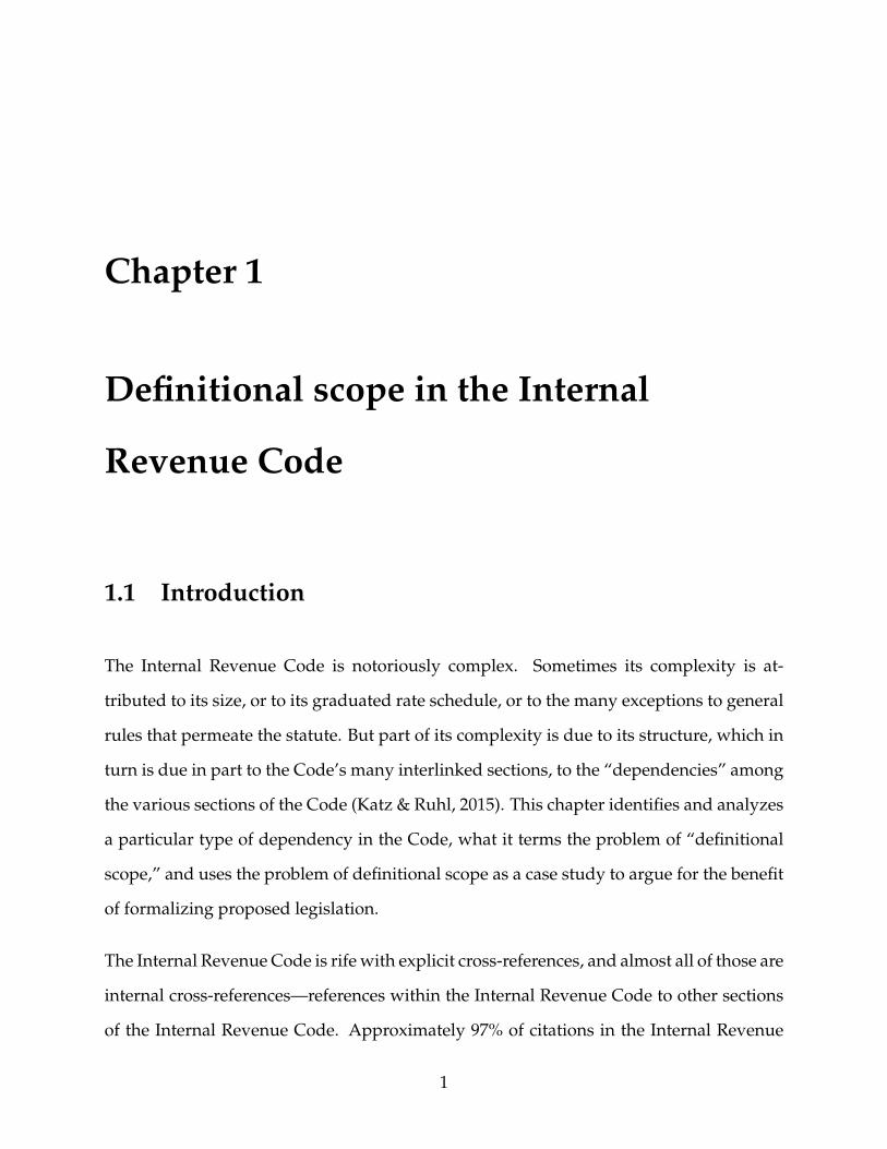
the number of shares redeemed ((Bernbach, 1955, p. 600), (Bittker, 1956, p. 39); see Fig-

ure 1.1.)

Figure 1.1: Correct Analysis

That said, continuing with the second redemption in the example, the corporation re-

deems 10 shares from Shareholder Y. At this point, if the math is worked out correctly,

Shareholder X fails both tests, because Shareholder X owns a slightly higher percentage

of the stock than he did originally, and also owns more than 50% of the stock. Share-

holder Y, on the other hand, fails the 80% test but not the 50% test. The legislative history

says that both have failed the test: “when the two transactions are reviewed together it

16

is apparent that [Shareholder X] and [Shareholder Y] have not sufficiently changed their

respective proportionate interests in the corporation.” This is an accurate statement re-

gardless of whether the 50% test is relevant, and indeed, this example sheds no light at

all on whether the 50% test is relevant (especially since one shareholder passes it and the

other fails).

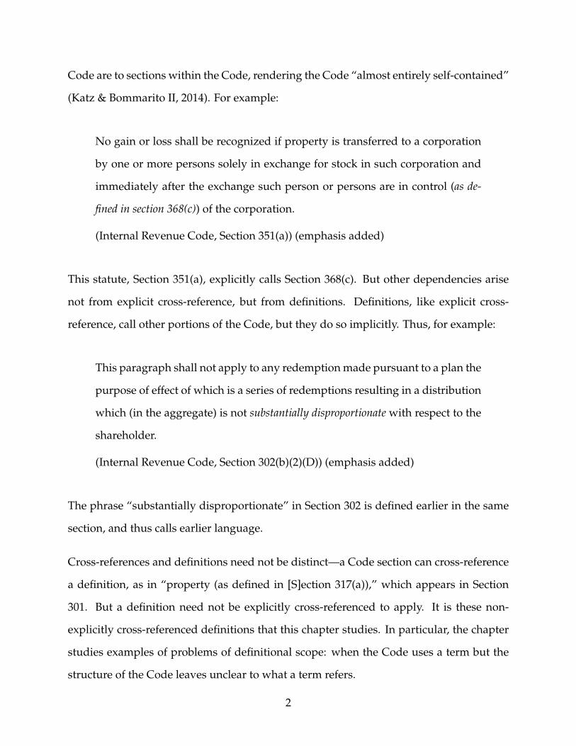
Because the legislative history does not work out the math correctly, one might wonder

whether this analysis is relevant at all. It is. If one assumes, as does Bittker, that the

Report is wrong because it fails to reduce the total number of shares in the corporation,

neither Shareholder X nor Shareholder Y fails either test after the second redemption. (See

Figure 1.2.)

Figure 1.2: Incorrect Analysis

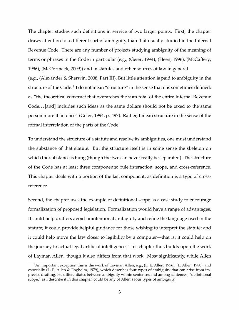
According to the legislative history, both shareholders fail the 80% test. For the numbers

to support this characterization, one must determine the shareholders’ respective per-

centage ownerships by not reducing the total number of shares in the corporation for the

first redemption, and then correctly reducing the total number of shares for the second

redemption (See Figure 1.3.)

17

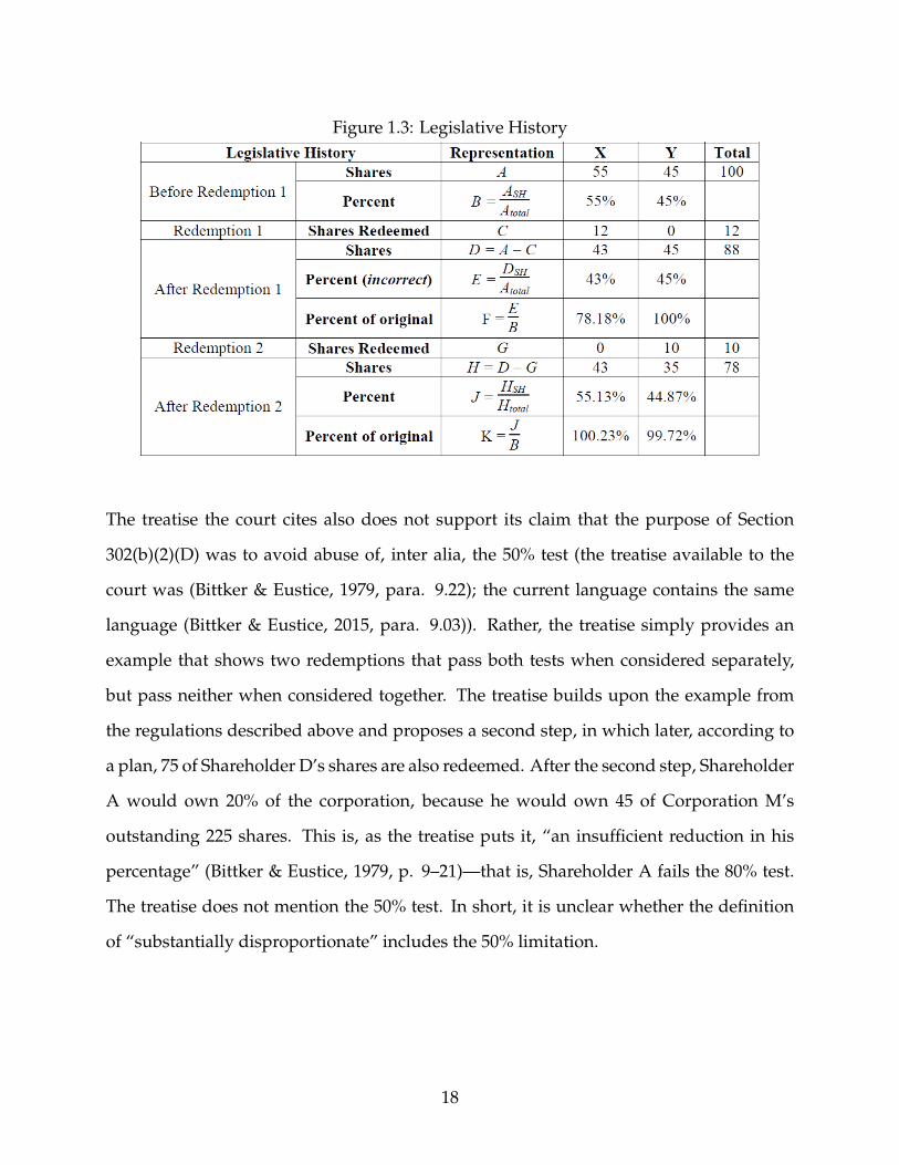
Figure 1.3: Legislative History

The treatise the court cites also does not support its claim that the purpose of Section

302(b)(2)(D) was to avoid abuse of, inter alia, the 50% test (the treatise available to the

court was (Bittker & Eustice, 1979, para. 9.22); the current language contains the same

language (Bittker & Eustice, 2015, para. 9.03)). Rather, the treatise simply provides an

example that shows two redemptions that pass both tests when considered separately,

but pass neither when considered together. The treatise builds upon the example from

the regulations described above and proposes a second step, in which later, according to

a plan, 75 of Shareholder D’s shares are also redeemed. After the second step, Shareholder

A would own 20% of the corporation, because he would own 45 of Corporation M’s

outstanding 225 shares. This is, as the treatise puts it, “an insufficient reduction in his

percentage” (Bittker & Eustice, 1979, p. 9–21)—that is, Shareholder A fails the 80% test.

The treatise does not mention the 50% test. In short, it is unclear whether the definition

of “substantially disproportionate” includes the 50% limitation.

18

1.2.3 Resolving problems of definitional scope

The ambiguities presented above could be resolved by drafting changes. Limitations

meant to be included in definitions can be incorporated into the respective “definitions”

sections. Limitations not meant to be included in later “calls” to the term can be explicitly

excluded in the later call, or the definition can be more precisely demarcated.

For example, if the definition of acquisition indebtedness is meant to include the $1 mil-

lion limitation, the statute could be redrafted as follows. (Changes have been made to the

definition of home equity indebtedness as well to maintain a parallel construction.)

(B) ACQUISITION INDEBTEDNESS.—The term “acquisition indebtedness” means any

indebtedness which—

(i) is incurred in acquiring, constructing, or substantially improving any qualified

residence of the taxpayer; and

(ii) is secured by such residence;

(iii) to the extent such indebtedness does not exceed $1,000,000.

(C) HOME EQUITY INDEBTEDNESS.—The term “home equity indebtedness” means

any indebtedness which

(i) is not acquisition indebtedness; and

(ii) is secured by a qualified residence;

(iii) to the extent the aggregate amount of such indebtedness does not exceed the

lesser of

(I) the fair market value of such qualified residence, reduced by the amount of ac-

19

quisition indebtedness with respect to such residence, and

(II) $100,000.

If, on the other hand, the $1 million limitation is not meant to be part of the definition

of acquisition indebtedness, the subsequent use of the term “acquisition indebtedness”

could make that clear by referring only to the relevant provisions. When the term is used

later, the Code could say explicitly that the term is to be defined by reference only to the

portion of the Code labeled “definition.” Thus the definition of acquisition indebtedness

could be left the same, but the definition of home equity indebtedness modified to read

as follows (new language in italics):

(i) In general.—The term “home equity indebtedness” means any indebtedness (other

than acquisition indebtedness (as defined in Section 163(h)(3)(B)(i)). . .

This explicitly calls the definitional language but omits the $1 million limitation, which

appears in Section 163(h)(3)(B)(ii).

Similarly, if the 50% limitation is meant to be part of the definition of substantially dispro-

portionate, the limitation could be included in the definitions section. Section 302(b)(2)(B),

the “Limitation” portion, could be deleted completely, and the new definition section

changed to read as follows:

(B) [OMITTED]

(C) DEFINITIONS.—For purposes of this paragraph, the distribution is substantially

disproportionate if—

(i)

(I) the ratio which the voting stock of the corporation owned by the shareholder

immediately after the redemption bears to all of the voting stock of the corporation

20

at such time,

is less than 80 percent of—

(II) the ratio which the voting stock of the corporation owned by the shareholder

immediately before the redemption bears to all the voting stock of the corporation

at such time;

(ii) immediately after the redemption the shareholder owns less than 50 percent of

the total combined voting power of all classes of stock entitled to vote; and

(iii) the shareholder’s ownership of the common stock of the corporation (whether

voting or nonvoting) after and before redemption also meets the 80 percent require-

ment of Section 302(b)(2)(C)(i).

If the 50% test is not meant to be included in the definition, Section 302(b)(2)(D) could

thus be rewritten (new language in italics):

This paragraph shall not apply to any redemption made pursuant to a plan the purpose

or effect of which is a series of redemptions resulting in a distribution which (in the

aggregate) is not substantially disproportionate (as defined in Section 302(b)(2)(C)) with

respect to the shareholder.

This excludes the 50% test, which appears in Section 302(b)(2)(B).

While fixing the law after it has been enacted is possible, preventing unintentional ambi-

guities from entering the law is preferable. The next section turns to the question of how

unintentional ambiguities can be avoided in future legislation.

21

1.3 A general solution: formalizing the Code

This section proposes that drafters3 should, as part of the process of drafting legislation,

formalize the proposed language.

For example, if the correct definition of a “substantially disproportionate” redemption

is a redemption that meets both the voting stock reduction test and the common stock

reduction test—but not necessarily the 50% test—one could write

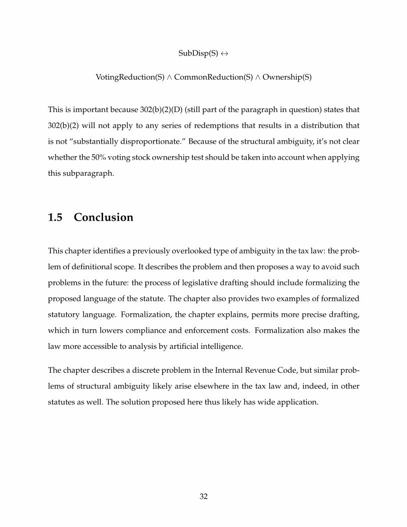
SubDisp(S)↔ (VotingReduction(S) ∧ CommonReduction(S))

This is only the first step in formalization. One would also have to define the various

predicates (VotingReduction(S), CommonReduction(S)). Section 1.4 includes a fuller for-

malization of the law.

The proposal here is not that the statute itself would include this formalization. Rather,

drafters would formalize proposed language to permit themselves to check the structure

of that language. Formalizing tax legislation will help prevent unintentional structural

ambiguity such as problems of definitional scope from making its way into the Code,

because formalization will force the drafters to notice the ambiguity. For example, as

noted above, if the correct definition of a “substantially disproportionate” redemption

is a redemption that meets both the voting stock reduction test and the common stock

reduction test, the proper formalization is as follows:

SubDisp(S)↔ (VotingReduction(S) ∧ CommonReduction(S))

On the other hand, if the correct definition of “substantially disproportionate” also in-

cludes the 50% test, the formalization would look like this:3Not Congressmen themselves, but professional drafters such as those who work for the Office of the

Legislative Counsel or the Joint Committee on Taxation.

22

SubDisp(S)↔

(VotingReduction(S) ∧ CommonReduction(S) ∧ Ownership(S))

where “Ownership(S)” indicates that the 50% ownership test is met with respect to Share-

holder S.

As Section 1.4 demonstrates more fully, it is not possible to formalize this Code section

without resolving which definition is correct. Formalizing the legislation would thus re-

quire drafters to be extremely precise about certain aspects of their drafting and would

prevent careless or unintentional ambiguity. One would imagine, for example, that had

the drafters attempted to formalize Section 302(b)(2), they would have noticed the am-

biguity and resolved it. The final formalization itself would not have been particularly

noteworthy; the benefit—avoidance of unintentional ambiguity—would have been gar-

nered from the act of formalization itself.

The act of formalization would therefore be helpful and desirable even if the formaliza-

tion were not published. If the formalization were published along with other legislative

history, however, other benefits could accrue. For example, a formalization could be use-

ful if a statute is particularly complex, as in some situations the formalization might be

easier to understand than the language of the statute, readers of the statute who need

to understand the statute’s structure more clearly could resort to the formalization. This

could be useful even in the absence of ambiguity. The formalization would not be bind-

ing. It would not itself be the legislation, and should be given the same weight, or lack of

weight, as any other legislative history.

Finally, formalizing statutes would help the project of applying artificial intelligence to

law. By “artificial intelligence,” I mean machines that can actually reason about the law,

not programs like TurboTax (as useful as such programs are) that simply translate tax

23

instruction forms onto a computer. The field of law and artificial intelligence is large

and ever-growing. Understandably, however, much of the work in this area is highly

theoretical and relatively untethered to the language of the law. Formalized statutory

language that tracks the actual structure of the law will make it easier for the theoretical

work and the law to converge. And when artificial intelligence does come to reason about

the law, it will only be as good as the inputs are accurate. Drafters’ formalizations will be

tremendously helpful in making those inputs as accurate as possible.

There are objections to the idea of formalizing proposed legislation, but none are particu-

larly persuasive. Three principal objections are as follows.

First, it may seem too complicated to ask drafters to formalize proposed legislation. But

even if the current staff would not be able to formalize the legislation, there are no short-

age of people who could be hired for the purpose of formalizing proposed language. The

formalization could be done by a separate group, perhaps within the Joint Committee on

Taxation, or a similarly nonpartisan, expert office. Moreover, legislative drafters are gen-

erally nonpartisan and increasingly sophisticated (Shobe, 2014). While formalization may

look daunting to some, in fact it is fairly easy to grasp. Even if drafters could not generate

formalizations themselves, they would soon acquire the ability to interpret them.

Second, and relatedly, it may seem too costly to formalize the language of statutes, and

the payoff may seem to be too small. Take the examples of problematic definitional scope

described above. They may seem minor, and at least one was eventually resolved. Would

avoiding them really have been worth hiring several extra staffers to translate proposed

language?

But the cost of formalizing must be weighed against the costs of not formalizing. That is,

the ex ante cost of avoiding structural ambiguity seems likely to be less than the ex post

cost of dealing with that ambiguity. The ex post cost includes not only litigation that could

24

have been avoided had the ambiguity been absent, but also increased compliance costs,

as even those who do not litigate must spend time and resources to resolve the ambiguity,

as well as audit costs, if the IRS disagrees with the approach some taxpayers have taken.

Formalization would join pre-enactment analyses such as cost estimates provided by the

Congressional Budget Office whose benefit has been deemed to outweigh their cost. Ad-

ditionally, approaches to drafting legislation are not static. As formalizers attempted to

formalize various proposed legislation, they would return to the drafters and ask them

to resolve ambiguities. The drafters might eventually learn how to write language that is

more easily formalized (i.e., clearer), and thus the cost of formalizing could become lower

over time.

Finally, one might object that what has here been characterized as problematic definitional

scope is in fact not a problem at all, and that more generally, Congress may sometimes

wish to leave obscure precisely what constitutes a definition. The familiar advantages

of ambiguity in legislation (e.g. (Grundfest & Pritchard, 2002), (Rosenkranz, 2002, pp.

2155–2156)) could apply just as easily to this sort of ambiguity. Perhaps the ambiguity

was intentional. Perhaps Congress could not resolve the issue, or perhaps it wished to

leave a gap in the statute—here, a structural gap, as it were, but a gap nonetheless—that

would later be filled by an administrative agency or the courts.

Given the mechanical, mathematical nature of the contexts in which these ambiguities

arise, it seems unlikely that the ambiguities are intentional. That is particularly true of

Section 302(b)(2), which was intended to provide a bright-line rule to allow taxpayers to

avoid resort to a facts-and-circumstances test (Bittker & Eustice, 2015, para. 9.01). How-

ever, formalization would not prevent drafters from including problems of definitional

scope in legislation. Indeed, more broadly, it would not prevent drafters from crafting

legislation that was structurally unclear or ambiguous. That the statute was formalized,

and that the formalization revealed an ambiguity, would in no way prevent such an am-

25

biguity from remaining in the legislation, just as knowing that a term in a statute is am-

biguous does not mean that the term is automatically removed.

Faced with an ambiguity, formalizers could publish alternate formalizations and indicate

that it was unclear from the language of the legislation which was correct. Or they could

choose not to publish a formalization of that portion of the statute, but rather publish an

explanation of why they could not formalize it. While formalization would not prevent

drafters from including ambiguities, it would help prevent drafters from including such

ambiguity unintentionally. While there may be advantages to ambiguity, drafters should

at the very least be able to make the conscious choice whether to include that ambiguity.

1.4 Formalizations

This Section provides possible examples of the formalization of the law described above.

As noted above, what follows is by no means the only possible way to formalize these

provisions.

1.4.1 Home mortgage interest deduction

Represent the taxpayer’s debt by an ordered triple:

α = 〈Purpose, Secured, Amount〉

(One could generalize even further, such that if the taxpayer has n debts, represent each

debt by αi, where 0 ≤ i ≤ n.)

Purpose is the purpose for which the debt was incurred, Secured is the property, if any,

that secures the debt, and Amount is the amount of the debt. Further, define the following

26

terms with respect to debt α:

Interest(α, Payment): Payment is an interest payment with respect to debt α = 〈Purpose,

Secured, Amount〉.

Purpose(α) (or, respectively, Secured(α), Amount(α)): project out the first (or, respectively

second, third) element of α, an ordered triple.

APurpose(x): Purpose x is to acquire, construct, or substantially improve a qualified res-

idence.

QRes(x): Residence x is a qualified residence.

AI(α) = AI(〈Purpose, Secured, Amount〉): 〈Purpose, Secured, AIAmount〉, where AIAmount

is the extent to which debt α is acquisition indebtedness.

HEI(α) = HEI(〈Purpose, Secured, Amount〉): 〈Purpose, Secured, HEIAmount〉, where

HEIAmount is the extent to which debt α is home equity indebtedness.

QRI(α, Payment): a payment, Payment, with respect to debt α is qualified residence inter-

est.

The obscurity arises immediately when attempting to define acquisition indebtedness. In

particular, is acquisition indebtedness to be defined in terms of amount, or only in terms

of purpose?

That is, would one say of debt α that the entire debt is acquisition indebtedness? Or

would one say that the debt is acquisition indebtedness only up to a certain amount? If

the government’s initial reading of the statute is correct, the statute would be formalized

as follows.

QRI(α, Payment)↔

27

Interest(AI(α), Payment) ∨ Interest(HEI(α), Payment)

Acquisition indebtedness would be defined as follows:

AI(α) = α↔

APurpose(Purpose(α)) ∧ QRes(Secured(α))

To define home equity indebtedness first define the preliminary term

TotalAI(r): the sum of all acquisition indebtedness with respect to a particular qualified

residence r.

Then define home equity indebtedness as follows (where “Min(x, y)” simply means “choose

the minimum of x and y,” and “FMV(x)” means “fair market value of x”):

HEI(α) = α↔

¬(AI(α) = α) ∧ QRes(Secured(α)) ∧

Amount(HEI(α)) = Min(Amount(α), (FMV(Secured(α)) − TotalAI(Secured(α)))

And, finally:

QRI(α, Payment)↔

(Min(Interest(AI(α), Payment), Interest($1,000,000, Payment))

∨

Min(Interest(HEI(α), Payment), Interest($100,000, Payment)))

28

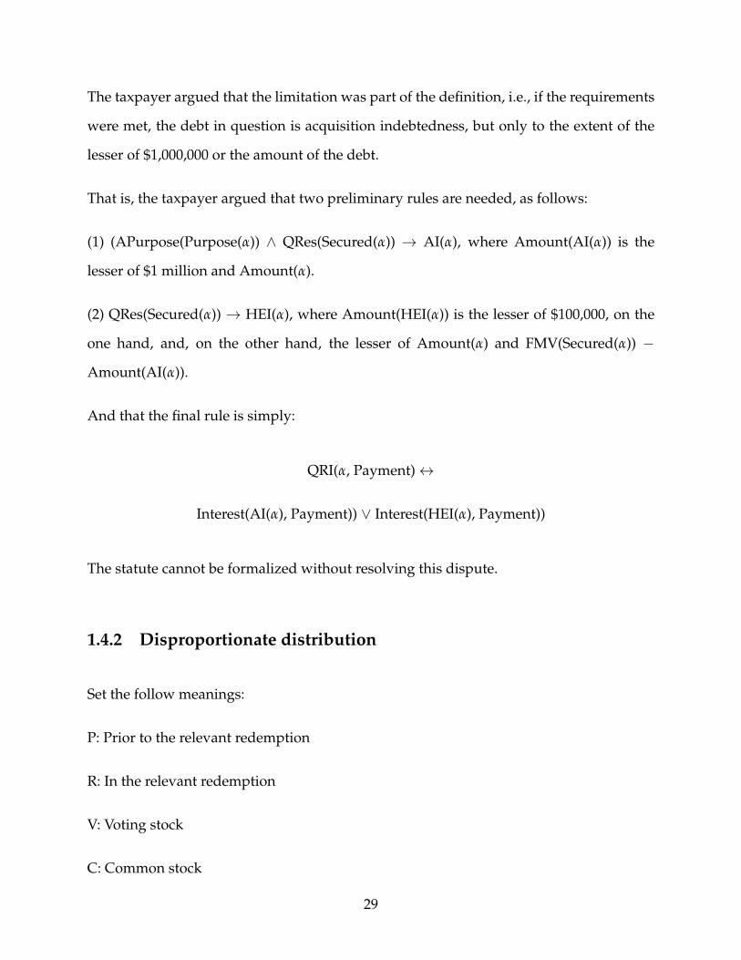
The taxpayer argued that the limitation was part of the definition, i.e., if the requirements

were met, the debt in question is acquisition indebtedness, but only to the extent of the

lesser of $1,000,000 or the amount of the debt.

That is, the taxpayer argued that two preliminary rules are needed, as follows:

(1) (APurpose(Purpose(α)) ∧ QRes(Secured(α)) → AI(α), where Amount(AI(α)) is the

lesser of $1 million and Amount(α).

(2) QRes(Secured(α)) → HEI(α), where Amount(HEI(α)) is the lesser of $100,000, on the

one hand, and, on the other hand, the lesser of Amount(α) and FMV(Secured(α)) −

Amount(AI(α)).

And that the final rule is simply:

QRI(α, Payment)↔

Interest(AI(α), Payment)) ∨ Interest(HEI(α), Payment))

The statute cannot be formalized without resolving this dispute.

1.4.2 Disproportionate distribution

Set the follow meanings:

P: Prior to the relevant redemption

R: In the relevant redemption

V: Voting stock

C: Common stock

29

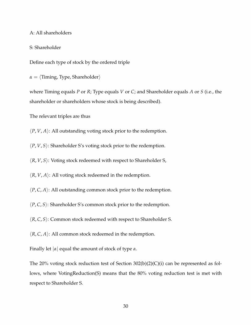
A: All shareholders

S: Shareholder

Define each type of stock by the ordered triple

α = 〈Timing, Type, Shareholder〉

where Timing equals P or R; Type equals V or C; and Shareholder equals A or S (i.e., the

shareholder or shareholders whose stock is being described).

The relevant triples are thus

〈P, V, A〉: All outstanding voting stock prior to the redemption.

〈P, V, S〉: Shareholder S’s voting stock prior to the redemption.

〈R, V, S〉: Voting stock redeemed with respect to Shareholder S,

〈R, V, A〉: All voting stock redeemed in the redemption.

〈P, C, A〉: All outstanding common stock prior to the redemption.

〈P, C, S〉: Shareholder S’s common stock prior to the redemption.

〈R, C, S〉: Common stock redeemed with respect to Shareholder S.

〈R, C, A〉: All common stock redeemed in the redemption.

Finally let |α| equal the amount of stock of type α.

The 20% voting stock reduction test of Section 302(b)(2)(C)(i) can be represented as fol-

lows, where VotingReduction(S) means that the 80% voting reduction test is met with

respect to Shareholder S.

30

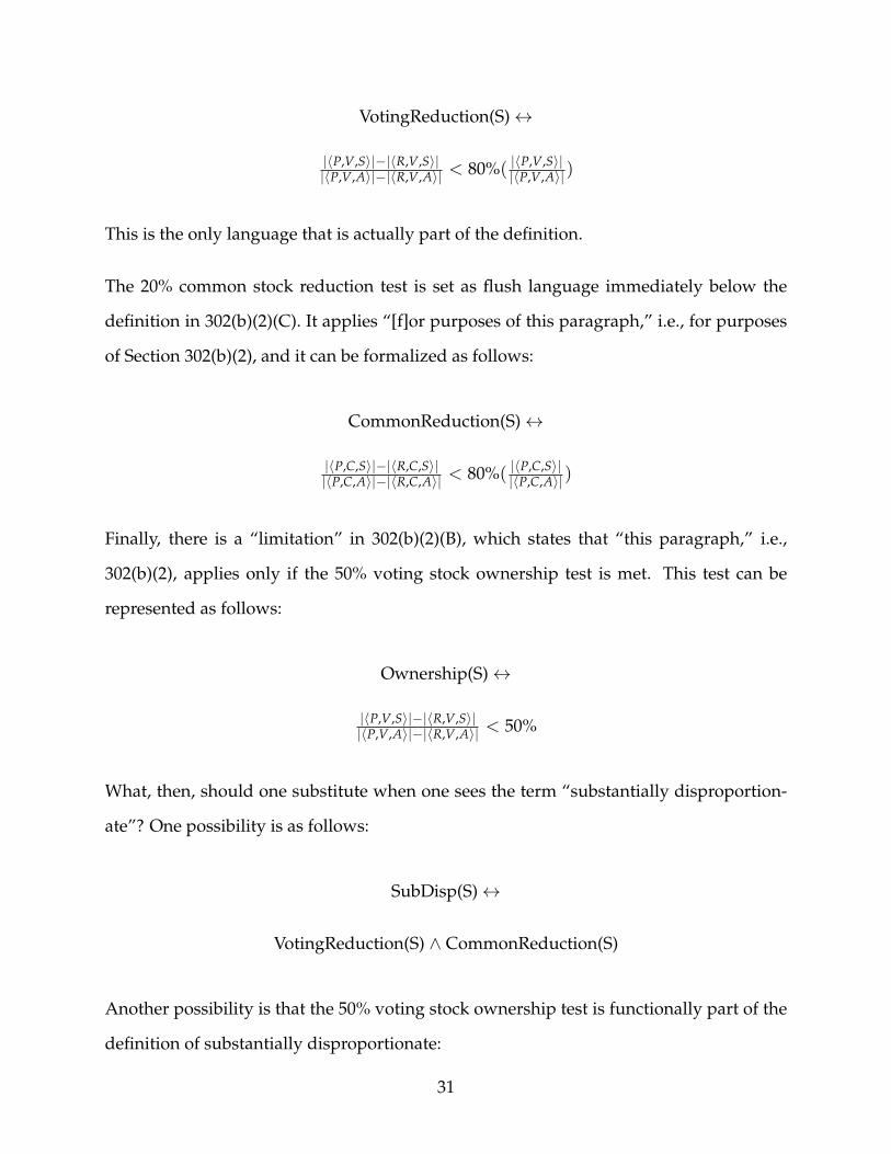
VotingReduction(S)↔

|〈P,V,S〉|−|〈R,V,S〉||〈P,V,A〉|−|〈R,V,A〉| < 80%( |〈P,V,S〉|

|〈P,V,A〉|)

This is the only language that is actually part of the definition.

The 20% common stock reduction test is set as flush language immediately below the

definition in 302(b)(2)(C). It applies “[f]or purposes of this paragraph,” i.e., for purposes

of Section 302(b)(2), and it can be formalized as follows:

CommonReduction(S)↔

|〈P,C,S〉|−|〈R,C,S〉||〈P,C,A〉|−|〈R,C,A〉| < 80%( |〈P,C,S〉|

|〈P,C,A〉|)

Finally, there is a “limitation” in 302(b)(2)(B), which states that “this paragraph,” i.e.,

302(b)(2), applies only if the 50% voting stock ownership test is met. This test can be

represented as follows:

Ownership(S)↔

|〈P,V,S〉|−|〈R,V,S〉||〈P,V,A〉|−|〈R,V,A〉| < 50%

What, then, should one substitute when one sees the term “substantially disproportion-

ate”? One possibility is as follows:

SubDisp(S)↔

VotingReduction(S) ∧ CommonReduction(S)

Another possibility is that the 50% voting stock ownership test is functionally part of the

definition of substantially disproportionate:

31

SubDisp(S)↔

VotingReduction(S) ∧ CommonReduction(S) ∧ Ownership(S)

This is important because 302(b)(2)(D) (still part of the paragraph in question) states that

302(b)(2) will not apply to any series of redemptions that results in a distribution that

is not “substantially disproportionate.” Because of the structural ambiguity, it’s not clear

whether the 50% voting stock ownership test should be taken into account when applying

this subparagraph.

1.5 Conclusion

This chapter identifies a previously overlooked type of ambiguity in the tax law: the prob-

lem of definitional scope. It describes the problem and then proposes a way to avoid such

problems in the future: the process of legislative drafting should include formalizing the

proposed language of the statute. The chapter also provides two examples of formalized

statutory language. Formalization, the chapter explains, permits more precise drafting,

which in turn lowers compliance and enforcement costs. Formalization also makes the

law more accessible to analysis by artificial intelligence.

The chapter describes a discrete problem in the Internal Revenue Code, but similar prob-

lems of structural ambiguity likely arise elsewhere in the tax law and, indeed, in other

statutes as well. The solution proposed here thus likely has wide application.

32

Chapter 2

Modeling rule-based legal reasoning

2.1 Introduction

Law in the United States is derived from, among other sources, cases (the “common law”)

and statutes. Common law reasoning is, without question, a puzzle. When students are

taught to ”think like lawyers” in their first year of law school, they are taught common

law reasoning. Books on legal reasoning—and there are many—are devoted almost en-

tirely to common law reasoning. How do courts reason from one case to the next? Is

common law reasoning reasoning from analogy? How should common law reasoning be

modeled? How can it be justified?

Statutory reasoning, in contrast, is taken as simple in legal scholarship. Statutory interpre-

tation—how to determine the meaning of words in a statute, the relevance of the lawmak-

ers’ intent, and so forth—is much discussed, but there is little treatment of the structure

of statutory reasoning once the meaning of the words is established. For example, the

chapter in (Alexander & Sherwin, 2008) entitled “Interpreting Statutes and Other Posited

Rules” addresses only the problems of interpreting the lawmaker’s intended meaning.

33

The actual reasoning underlying statutory analysis is disposed of in just two pages: statu-

tory reasoning simply involves following rules. Statutory reasoning is difficult only to the

extent that understanding a term in the statute is difficult, and the meaning of the term,

they explain, will be determined by a court, which throws us right back into common

law reasoning. (Levi, 1949) deals with statutory reasoning in a similarly cursory fashion:

statutory reasoning is often considered deductive, he explains, and, while this may not

be true, it is a useful approach; any complications that arise come from “ambiguity in the

words used” (Levi, 1949, p. 28).

This chapter examines the structure of statutory reasoning after ambiguities are resolved

and the meaning of the statute’s terms established. For statutory reasoning is not best un-

derstood as merely deductive. And while statutory reasoning can be fruitfully modeled

using formal logic, standard formal logic is not the best approach for modeling statutory

reasoning. Rather, this chapter argues, using the Internal Revenue Code and accompany-

ing regulations, judicial decisions, and rulings as its primary example, that at least some

statutory reasoning is best characterized as defeasible reasoning—reasoning that may re-

sult in conclusions that can be defeated by subsequent information—and is best modeled

using default logic.

A range of literature argues that legal reasoning is best understood as defeasible reason-

ing, including (Prakken & Sartor, 2004), (Hage, 2003), (Sartor, 1992), and (Sartor, 1994).

Indeed, the word “defeasibility” is borrowed from the law; the term dates back at least

to (Hart, 1948). The belief revision project of Alchourron, Gardenfors, and Makinson, de-

scribed in (Gardenfors, 2003), began as a way to model legal reasoning. Yet these sources

generally (though not entirely) neglect the intrinsic defeasibility of statutory reasoning.

For example, (Gardenfors, 2003) takes legal codes as “a set of propositions together with

their logical consequences” (Gardenfors, 2003, p. 101). Belief revision is relevant to un-

derstanding legal codes, but only because rules are added and removed. (Hage, 2003)

34

argues that legal reasoning may be defeasible, but his reasons for defeasibility include

only that the burden of proof or the process of discovery may introduce new information,

and that extralegal considerations may include implied exceptions to the law. (Walker,

2007) argues for the application of default logic to the law, but limits his discussion to

reasoning about evidence (fact-finding). There are a few examples of defeasible statutory

reasoning in the literature. (Horty, 2012), for example, provides a fictional example of a

conflict between a federal and state statute to illustrate default reasoning. This chapter

takes a similar approach, but instead of using a fictional example, it draws from an actual

statute and demonstrates defeasibility intrinsic to the statute itself.

2.2 Defeasible reasoning and default logic

Once deductive reasoning provides a conclusion, nothing within deductive reasoning

can unseat that conclusion. Consider a very basic deductive argument: “If A, then B.

A. Therefore, B.” Given A, no additional information can shake the reasoner from B. (Of

course, changing the information one has can change the conclusion. ”I thought that if A,

then B. But I was wrong. So although I have A, I cannot conclude B.”) Because conclusions

arrived at through deductive reasoning cannot be defeated by additional information,

such conclusions are indefeasible.

Most everyday reasoning, in contrast, leads to defeasible conclusions, conclusions that

might be defeated by additional information. Defeasible reasoning is sometimes referred

to as the logic of jumping to conclusions. In the classic example, someone learns that

Tweety is a bird and concludes that Tweety can fly. But this conclusion is defeasible, be-

cause additional information could cause the reasoner to change his mind. For example,

if the reasoner learns that Tweety is is a penguin, he will conclude that Tweety can’t in

fact fly.

35

Because deductive logic is indefeasible—regardless of additional information, a conclu-

sion, once reached, will not be rejected—the formalization of deductive logic (“standard

logic”) is monotonic. That is, for any sets of propositional formulas Γ, ∆, and some for-

mula ϕ, if Γ ` ϕ, and Γ ⊆ ∆, necessarily ∆ ` ϕ.

In contrast, formalized defeasible logic is nonmonotonic. That is, where we take |∼ to

mean “defeasibly prove,” or “tend to show,” if Γ |∼ ϕ, and Γ ⊂ ∆, it is not necessarily true

that ∆ |∼ ϕ. Return to Tweety. Where P means “Tweety is a penguin,” B means “Tweety

is a bird,” and F means “Tweety can fly,” represent the situation in which we know that

Tweety is a bird as Γ = {B}. Conclude, defeasibly, that Tweety can fly, i.e., B |∼ F. But

now consider the expanded belief set ∆ = {B, P}, i.e., Tweety is a bird and Tweety is a

penguin. Γ ⊂ ∆, but penguins can’t fly, so this expanded belief set no longer supports

jumping to the conclusion that Tweety can fly, i.e., ∆ 6 |∼ F, and in fact, the expanded

belief set supports the conclusion that Tweety can’t fly, ∆ |∼ ¬F. This is nonmonotonic

reasoning: we reject an earlier conclusion (F) because of additional information (P).

There are a variety of ways to formalize nomonotonic reasoning. This chapter uses a

variant of default logic, which was originally developed in (Reiter, 1980). Under this

approach, the reasoner has a set of propositional formulas,W , which we can informally

think of as a world; default rules, δ ∈ D; and a relationship between the default rules,

<. The relationship establishes the relative priority of the default rules—which rule takes

precedence over another—and thus this approach is a type of prioritized default logic.

For example, consider trying to determine whether a particular person—call him Henry—

can read. If the only information you have is that Henry lives in the United States

(“UnitedStates”), you should conclude that he can read (“Read”). (According to

(Central Intelligence Agency, 2014), approximately 99% of the U.S. population older than

14 can read, and according to (U.S. Census Bureau, 2010), 80% of the U.S. population

is older than 14.) If you learn, however, that Henry is five years old, you should con-

36

clude he cannot read, as most children in the United States do not read before age six

(call younger than age six “Young”). These two rules together give us our set ∆ of default

rules, rules that might be defeated by each other or by other rules. These rules don’t apply

with certainty, but in general they are good guides to reasoning. If we have no additional

information, ∆ = (W, D,<), where

W = ∅

D = {δ1, δ2}

δ2 : UnitedStates ⊃ Read

δ1 : Young ⊃ ¬Read

<: δ1 < δ2

The “lower” the rule, the stronger, so here, δ1 dominates δ2. That is, if both might apply,

δ1 “beats” δ2.1

This chapter uses an “order of application” variant of default logic. As argued in Chap-

ter 4, statutory rules are best considered supernormal, which permits the use of a modi-

fied (simplified) version of (Brewka & Eiter, 2000): consider the default rules from strongest

to weakest, adding to the set of things one should believe the rule we are considering at

each stage if that rule is consistent with already adopted beliefs. Because the rules are

considered from strongest to weakest, stronger rules will keep out weaker, inconsistent

rules. And the belief set will itself be consistent, because a rule can be added only if it is

consistent with what one already believes.

Formally, consider a fully-prioritized default theory ∆ = (D, W,<), where < is a well

1In contrast to the approach in Horty’s work, described infra, here the lower rule must dominate thehigher rule. As described below, construction of the set of accepted rules proceeds recursively, fromstrongest to weakest, and so the well-ordering here serves to ensure that one can always pick the strongestrule remaining.

37

ordering on D. That is, < is irreflexive and transitive with respect to the default rules,

and any non-empty subset of default rules has a least element.

In (Brewka & Eiter, 2000), each default rule d is of the form a : b1, . . . bn/c, where n ≥ 1,

which means that given a, if b1 . . . bn is consistent with what has already been accepted,

then (defeasibly) conclude c. Each a, b, and c is a first-order formula. Call a the prereq-

uisite, the bi formulas the justifications, and c the consequent. Define functions pre(d),

just(d), and cons(d) to pick out the prerequisite, the set of justifications, and consequent,

respectively, of d. Define ¬ just(d) = {¬a|a ∈ just(d)}.

A default rule d = a : b/c is normal if b is logically equivalent to c. A default rule d

is prerequisite-free if a is a logical truth, >. A rule that is normal and prerequisite-free is

supernormal. A supernormal default rule is of the form : c/c, and can be taken to mean “if c

is consistent with has already been derived, conclude c.” Because, as argued in Chapter 4,

statutory rules are best considered as supernormal, write a default rule representing a

statutory rule as a formula c. Writing a default rule d = a : b/c as c should be taken to

mean, in Brewka and Eiter’s terms, that pre(d) = a = >, just(d) is logically equivalent to

c, and cons(d) = c.

For a set of formulas S, a default c is active in S if ¬ just(d)∩ S = ¬{c} ∩ S = ∅ and c /∈ S.

(Recall that we write c for the elements of the set of justifications instead of d because the

rule is supernormal and just(d) is logically equivalent to c.) That is, c is consistent with S,

and c has not yet been applied.

Additionally simplify the Brewka and Eiter approach because there are a countable, in-

deed, a finite number of laws. Define an operator C (modified from (Brewka & Eiter,

2000)):

C(∆) =⋃

α≥0 Eα, where E0 = Th(W). That is, E0 is the set of all formulas that are classi-

cally entailed by W (i.e., provable from W using standard monotonic logic).

38

For every natural number α ≥ 0,

Eα+1 =

Eα if no default from D is active in Eα

Th(Eα ∪ {d}) otherwise, where d = min<{d′ ∈ D|d′ is active in Eα}

Brewka and Eiter posit that the set of rules a reasoner should adopt is the preferred ex-

tension of ∆, where E is the preferred extension of ∆ exactly when E = C(∆). (There is

always exactly one preferred extension, because there is only one way to proceed through

the construction process. At any step, because < is a well ordering, there is either a single

least element in the set of rules that are active, or there are no rules left that are active.)

The general idea is that a rule applies unless it is defeated by a higher-priority rule.

For example, return to the literacy question. Suppose we are told that Henry is from the

United States (“UnitedStates”) and is four years old (“Young”). Now ∆ = (W, D,<),

where

W = {UnitedStates, Young}

D = {δ1, δ2}

δ2 : UnitedStates ⊃ Read

δ1 : Young ⊃ ¬Read

<: δ1 < δ2

E0 = Th(W) = Th({UnitedStates, Young})

The most powerful active rule in E0, i.e., the highest priority (lowest ranked) rule consis-

tent with E0 and not yet applied, is δ1 : Young ⊃ ¬Read. Therefore,

E1 = Th(W ∪ {Young ⊃ ¬Read})

39

While δ2 is not yet part of the belief set, it is not active, because it is inconsistent with E1.

In particular,

¬{UnitedStates ⊃ Read} ∩ Th(W ∪ {Young ⊃ ¬Read}) =

{UnitedStates∧¬Read} ∩ Th(W ∪ {Young ⊃ ¬Read}) =

{UnitedStates∧¬Read} 6= ∅

Therefore, En = E1 for n ≥ 1, and C(∆) =⋃

α≥0 Eα = E1. Thus, under Brewka and Eiter’s

approach, a reasoner should adopt the set of beliefs that are derived from W ∪ {Young ⊃

¬Read} and conclude, defeasibly, that Henry cannot read.

A legal example helps show why this approach to formalizing defeasible reasoning cap-

tures statutory reasoning well.

2.3 Formalizing Section 163

This section further formalizes the law described in Section 1.2.1. As described in that

section, the relevant law provides three main rules with regard to the deductibility of

interest.

First, in general, interest payments (“Interest”) are deductible (“Deductible”).

δ3 : Interest ⊃ Deductible

Second, even though in general interest payments are deductible, personal interest pay-

ments (“Personal”) are in general not deductible.

40

δ2 : Personal ⊃ ¬Deductible

And, finally, even though personal interest payments are in general not deductible, if

the personal interest payments are payments of qualified residence interest (“QRI”), then

those payments are deductible. Even though no rule within Section 163 suggests that this

rule is defeasible, it is defeasible, because other rules in the Internal Revenue Code may

defeat it.

δ1 : QRI ⊃ Deductible

It may seem that δ1 does not track the Code. According to the Code, “personal” interest

does not include, inter alia, qualified residence interest. So the Code embeds the exception

for qualified residence interest within the definition of personal. But, notwithstanding the

language of the Code, qualified residence interest is conceptually an exception to the rule

that personal interest is not deductible. This is how court opinions, treatises, and the

legislative history characterize the rule, even as they accurately reflect its placement in

the Code. I provide a few examples below, selected almost at random from the relevant

pool of sources; each of these examples could be multiplied.

In Pau v. Commissioner, the Tax Court states, “Section 163(h) disallows personal interest

deductions unless they fit within certain narrowly prescribed categories. Among these

narrow exceptions is the deduction for interest on a qualified residence.” Of course, by

the language of the Code, Section 163(h) simply disallows what it defines as personal in-

terest deductions, and deductions for interest on a qualified residence is not a personal

interest deduction. But notwithstanding the structure of the Code, the court reads the

41

home mortgage interest deduction as an exception to the personal interest rule. Simi-

larly, a leading federal income taxation treatise states, “Personal interest is nondeductible

under [Section] 163(h), unless it is ’qualified residence interest’ ” (Bittker, McMahon, &

Zelenak, 1995, Section 18.04). Again, strictly speaking, from the structure of the Code,

personal interest is nondeductible, and personal interest does not include qualified resi-

dence income.

The history of current Section 163(h) also reflects the home mortgage interest deduction

as an exception from the general rule that personal interest is not deductible. In the tax

reform proposal that limited personal interest deductions, the change in law was de-

scribed as limiting the deduction of “all interest not incurred in connection with a trade

or business (other than interest on debt secured by the taxpayer’s principal residence. . . )”

(Reagan, 1985, p. 323). (For a general discussion of the history of the mortgage interest

deduction that clearly reflects that the deduction is an exception to the general rule that

personal interest is not deductible, see (Ventry, 2010).)

Additionally, order the rules, defining < : δ1 < δ2, δ2 < δ3. That is, δ1 dominates δ2, δ2

dominates δ3, and by transitivity δ1 dominates δ3.

There are also two statements that are certain (essentially, they are definitional) and thus

go in W (additional information may also go in W): personal interest payments are always

interest payments, and qualified residence interest payments are always personal:

Personal ⊃ Interest

QRI ⊃ Personal

Thus:

42

W = {Personal ⊃ Interest, QRI ⊃ Personal}

δ3 : Interest ⊃ Deductible

δ2 : Personal ⊃ ¬Deductible

δ1 : QRI ⊃ Deductible

<: δ1 < δ2 < δ3

This ∆ = (W, D,<) shows the general structure of the system of rules. Formally defining

these terms adds a level of complication, as described in Chapter 1, but at heart, these

rules provide the structure of Section 163(h). (One might argue that there are four rele-

vant rules, and that one should consider that in general, payments are not deductible—

that is, without an explicit statutory authorization, no deduction may be taken. I.e., add

Interest ⊃ Payment to W, and δ0 : Payment ⊃ ¬Deductible to ∆. But for our purposes,

these three suffice.)

To see how these rules combine, take, for example, the situation in which an individ-

ual makes a payment of personal interest, and there is no evidence that the payment is

qualified residence interest.

W = {Personal ⊃ Interest, QRI ⊃ Personal, Personal}

E0 = Th(W) =

Th({Personal ⊃ Interest, QRI ⊃ Personal, Personal})

The first rule to consider is δ1 : QRI ⊃ Deductible. This rule is consistent with E0 =

Th(W) and has not yet been applied. Therefore, add it to E0 in order to obtain E1. (It may

seem strange to have this rule in our belief set, as it does not seem relevant. In fact, it is

43

critical that we include it, as in other scenarios it will prevent the problem of, for example,

the Order Puzzle from arising. For more on this see Chapter 5.) Thus:

E1 = Th(W ∪ {δ1}) =

Th({Personal ⊃ Interest, QRI ⊃ Personal, Personal, Interest, QRI ⊃ Deductible})

Next consider δ2 : Personal ⊃ ¬Deductible. This rule is consistent with Th(E1), so add it

as well.

E2 = Th(E1 ∪ {δ2}) =

Th({Personal ⊃ Interest, QRI ⊃ Personal, Personal, Interest,

QRI ⊃ Deductible, Personal ⊃ ¬Deductible})

Next, δ3, which is not consistent with E2, because ¬(Interest ⊃ Deductible) ∈ E2.

There are no more rules to apply, and the union of all the Eα is, obviously, equal to E2.

Therefore the preferred extension E of ∆ is Th(W ∪ {δ1, δ2}). ¬Deductible ∈ Th(W ∪

{δ1, δ2}). Therefore, the interest payment in question is not deductible.

2.4 The benefits of nonmonotonicity

Nonmonotonic logic isn’t necessary for representing defeasible reasoning (Alchourron,

1993, e.g.). Take Section 163, for example. One arrives at the correct answer (deductible

or not deductible) with just these two rules, in standard monotonic logic:

44

Interest∧(¬Personal∨QRI) ⊃ Deductible

Interest∧Personal∧¬QRI ⊃ ¬Deductible

Thus (Dworkin, 1967) proposes that rules are “all or nothing”: an “accurate” statement

of a rule takes all exceptions into account and “legal consequences follow automatically”

(Dworkin, 1967, p. 25).

Or perhaps the choice between representing statutory reasoning using, on the one hand,

a nonmonotonic logic, or, on the other, a monotonic logic is a false choice: other non-

standard logics may actually be better suited to represent statutory reasoning. For ex-

ample, (Nolt, Gray, MacLennan, & Ploch, 1995) propose a logic for statutory law based

on relevance logic, which adds constraints to the conditional in order to require a tighter

connection relation between the antcedent and the consequent (Priest, 2008, e.g. ch. 10).

But my claim isn’t that nonmonotonic logic is required to represent statutory reasoning,

but rather that nonmonotonic logic is preferable for formalizing the Code, as compared

both to standard nonmonotonic logic and to other nonstandard logics. As (Hage, 2005)

puts it, whether to use nonmonotonic logic in a particular situation is a question of prag-

matics. What logic is best depends on one’s purpose. (Nolt et al., 1995), for example, aims

to find a logic that permits artificial intelligence to reach accurate legal conclusions (Nolt

et al., 1995, p. 122). (Nolt et al., 1995) does not track extant statutory structure, but for

their purpose, whether the logic accurately reflects, for example, the statutory structure

is of little interest. But in the case of statutory reasoning, the pragmatics is on the side of

nonmonotonic logic, for at least three reasons. I use Section 163 as the example here, but

again, Section 163 is in no way unique.

First, strictly speaking, some metarule is required to know how to apply the rules of Sec-

45

tion 163, because on their face, the rules of Section 163 are inconsistent. Section 163(a)

states simply, “There shall be allowed as a deduction all interest paid or accrued within

the taxable year on indebtedness.” It does not say, for example, “except as otherwise stated

in this Section, there shall be allowed as a deduction all interest paid. . . .” (There are sec-

tions of the Code that contain explicit carveouts; for example, Section 61 states, “Except

as otherwise provided in this subtitle, gross income means. . . .” But Section 163(a) does

not contain such language.)

Section 163(h) seems, again, strictly speaking, inconsistent with the rule in Section 163(a):

“In the case of a taxpayer other than a corporation, no deduction shall be allowed . . . for

personal interest paid or accrued during the taxable year.” How is one to reconcile “there

shall be allowed as a deduction all interest” with ”no deduction shall be allowed . . . for

personal interest”? The statute itself does not tell us. Of course, this is not difficult to

resolve: the more specific rule (Section 163(h)) dominates the more general rule (Section

163(a)). But simply on the statute’s face, deductive logic is not sufficient to represent the

rules, because deductive logic provides no tools for resolving the (apparent) inconsistency

of the statute.

The metarules that resolve this problem, and others like it, are called “canons of statutory

interpretation.” While many of the canons help resolve ambiguities in the language of

the statute, and thus do not properly apply to the task of this chapter, others are relevant,

such as the canon that the more specific rule controls. (As (Llewellyn, 1949) notes, the

canons can have a “thrust and parry” nature, with many canons having an equal and

opposite canon—but in the core cases canons can resolve conflicts.)

This is consistent with the approach of (Dworkin, 1967) to rules:

[W]e cannot say that one rule is more important than another within the sys-

tem of rules, so that when two rules conflict one supercedes the other by virtue

46

of its greater weight. If two rules conflict, one of them cannot be a valid rule.

The decision as to which is valid, and which must be abandoned or recast,

must be made by appealing to considerations beyond the rules themselves. A

legal system might regulate such conflicts by other rules, which prefer the rule

enacted by the higher authority, or the rule enacted later, or the more specific

rule, or something of that sort. A legal system may also prefer the rule sup-

ported by the more important principles. (Our own legal system uses both of

these techniques.)

(Dworkin, 1967, p. 27)

This description of appealing to other rules outside the system to decide which rule is

to be discarded (overridden) is exactly the approach of defeasible reasoning and default

logic. (Dworkin, 1967) characterizes the abandoned rule as “not valid,” but it is perhaps

more accurate to say that in a given situation, a particular rule might not apply because it

is dominated by another rule.

Second, and relatedly, some rules are not contained in the Code. Consider the debate

in Pau v. Commissioner and described in Chapter 1. Is the $1 million limitation part of

the definition of acquisition indebtedness, or is it not? The Tax Court, in Pau v. Commis-

sioner, held that it was not. But the Internal Revenue Service declined to follow Pau v.

Commissioner and issued a revenue ruling that stated, effectively, that the IRS would treat

the $1,000,000 limitation as part of the definition (Internal Revenue Service, 2010). Which

advice should a lawyer give a taxpayer? Should the lawyer recommend that the client

follow the court’s ruling on the one hand, or the (opposite) revenue ruling on the other?

(Notice that this is not an ambiguity in the meaning of the terms of the statute, but rather

in the structure of the statute itself.) To resolve the dilemma, the lawyer will take into ac-

count the extra-statutory rule that the revenue ruling means that the IRS, which is charged

with enforcing the tax law and would be the agency to pursue the taxpayer were he to file

47

incorrectly, is committing not to pursue the taxpayer if he takes the approach described in

the revenue ruling. In other words, the taxpayer-favorable revenue ruling controls. There

are many sources of authority for interpreting statutes—different levels of government

(federal, state, local); within each level, there may be different branches of government

(legislative, judicial, administrative); and within each branch, different strengths of au-

thority (for example, district court, appeals courts, and so forth). One must know how

to resolve conflicts among these various authorities to apply statutes correctly, and for

the most part, the relative strength of these authorities is not contained in the statute one

attempts to interpret.

Finally, even if the Code did say “except as otherwise stated in this Section, there shall be

allowed as a deduction all interest paid. . . ,” and even if no authorities conflicted, to take

the deductive approach would lose the structure of the Code. The Code is not flat. Sec-

tion 163 itself is not flat: Section 163(a) is the “general rule” (that is its title), with various

subrules and exceptions that follow. And it is itself embedded in a title (Title 26, which in-

cludes all tax law), a subtitle (Subtitle A, income taxes), chapter (Chapter 1—normal taxes

and surtaxes), subchapter (Subchapter B—computation of taxable income), and part (Part

VI—itemized deductions for individuals and corporations). These divisions are far from

incidental. The law itself is defined by these groupings, as some sections include def-

initions “for purposes of this Part,” or “for purposes of this Subchapter,” and so forth.

Financial consequences of these groupings can be significant: when the net investment

income tax (“NIIT”) was created in 2013, it was placed in Chapter 2A of the Code, thus

making NIIT payments ineligible for the foreign tax credit. By its terms, the foreign tax

credit is available only for taxes imposed by “this chapter” (Section 901). Because of the

location of Section 901, the credit is available only for those taxes imposed by Chapter 1

of the Code. And neither are the NIIT payments covered by social security totalization

treaties, which apply only to those taxes imposed by Chapter 2 of the Code. These limi-

tations, and the resulting double tax, are apparent nowhere on the face of the statute, but

48

entirely due to the location of the NIIT in the Code. The Code’s structure matters. (There

is even a map of the income tax code, (Motri & Schenk, 2013).)

It’s not surprising that default logic accurately reflects the statutory structure, as the

general-to-specific approach (general rules followed by exceptions) is the approach rec-

ommended to legislative drafters. For example, (Forstater, 1995), a manual created by the

office in the House of Representatives that drafts legislation and intended as a “guide-

book for individuals who are undergoing. . . on-the-job drafting training,” urges drafters

to follow, as much as possible, a general-to-specific organization:

Before choosing an organization for a draft, determine to what extent it could

appropriately fit into the following arrangement:

(1) General rule.—State the main message.

(2) Exceptions.—State the persons or things to which the main message does

not apply.

(3) Special rules.—Describe the person or things—

(A) to which the main message applies in a different way; or

(B) for which there is a different message.

(Forstater, 1995, p. 23)

The Senate legislative drafting manual contains a similar exhortation:

In General—A section contains some or all of the following provisions and is

organized as follows:

SEC. 101. SECTION HEADING.

49

(a) DEFINITIONS.

(b) GENERAL RULE.

(c) EXCEPTIONS.

(d) SPECIAL RULES.

(Office of the Legislative Counsel, United States Senate, 1997, p. 10)

This organization—of general rule followed by exceptions—is exactly the structure fol-

lowed by default logic. And it is also how people describe the law: in Revenue Ruling

2010-25, for example, the IRS begins by stating the general rule (a deduction is allowed

for interest payments), then introduces the first exception (there is no deduction for per-

sonal interest) and then the last exception, the least general rule (there is a deduction for

qualified residence interest). The same approach appears in any textbook (Schmalbeck et

al., 2015, e.g. pp. 381–385), treatise (Bittker et al., 1995, e.g. Section 18.04), or case (e.g.

Pau v. Commissioner).2 The next section describes the benefits of formalization’s tracking

the structure of the statute.

2.5 Conclusion: The benefits of default logic

Because default logic more accurately reflects the structure of statutes and the practice

of rule-based legal reasoning than does standard logic, using default logic to represent

rule-based legal reasoning in general, and statutory reasoning in particular, has both the-

oretical and practical benefits.2A caveat: Although nonmonotonic logic is better suited to modeling rule-based legal reasoning than are

other logics, nonmonotonic logic does not perfectly map a human’s reasoning about legal rules. Perhaps thelargest problem is that human reasoning about legal rules, at least as represented in court cases, treatises,and rulings, tends to work from the most general rule to the most specific, the opposite direction of themodified Brewka-Eiter approach. While general-to-specific may not be the most efficient way to arrive at aconclusion about whether a particular payment is deductible, it is the way to explain the rules that makesmost sense to a person.

50

2.5.1 Theory

Using default logic to represent rule-based legal reasoning highlights the conceptual cat-

egory rule priority, a category that crosscuts legal reasoning and is implicit to what much

of lawyers do, but remains undertheorized.

As an initial matter, certain types of rule priority seem obvious. A statute (for example)

obviously dominates, say, a notice from the Internal Revenue Service. In some sense this

is accurate; a statute is enacted by Congress and signed by the President, whereas a notice

is simply a statement of how an administrative agency will administer the law. On the

other hand, if the enforcer tells you that it will not enforce the law, then it seems safe to

violate the law, and the enforcer’s notice dominates the statute. This is precisely what

happened when, for example, in Notice 2008-76, the Internal Revenue Service announced

that it would not enforce a provision of Section 382 against banks, effectively transferring

over $100 billion to certain private parties in violation of explicit, clear statutory law. No

lawyer would advise his client to follow the statute and not the notice.

More generally, in many situations there may be a variety of different “right” answers

to a question of law, depending on the precise question one is asking. The right answer

might be, for example, “the answer that is most compliant with the law,” or the right

answer might be “the advice that a tax lawyer should give a risk-averse client,” or the

right answer might be “the conclusion a judge would reach.” Default logic’s formaliza-

tion will in fact be able to provide any of those three answers (and others!), even though

the answers might be different than one another, depending on the priority the formal-

izer gives to the various rules. A tax lawyer giving advice to a client would, for example,

give an IRS ruling higher priority than a Supreme Court opinion that held to the contrary,

notwithstanding that a Supreme Court opinion has, in some very important sense, more

authority.

51

Conceiving of rule-based legal reasoning as defeasible reasoning, reasoning that is best

formalized by a nonmonotonic logic such as default logic, thus suggests another area, rule

priority, in which the classic answers to questions of statutory interpretation may apply. A

familiar argument relating to statutory interpretation is that interpreting statutes depends

primarily not on logic, but on norms. As (Sunstein, 1990) writes: “[E]xtratextual norms—

understood as principles about constitutional government, institutional arrangements,

basic fairness, and regulatory failure—do in fact play a crucial role in the interpretation

of statutes. Indeed, descriptive and prescriptive work on this topic is impossible without

an understanding of norms” (Sunstein, 1990, p. 803). And (Dworkin, 1975) explains

that “the calculations judges make about the purposes of statutes are calculations about

political rights” (Dworkin, 1975, p. 1086).

At first glance, this objection—that norms, not logic, are relevant to understanding statu-

tory reasoning—seems to conflate interpretation and reasoning. The former, the explicit

subject of Sunstein’s and Dworkin’s inquiry, involves determining the meaning of statu-

tory language and filling gaps left by the legislature. As Sunstein describes the task of in-

terpretation, courts must handle “statutory language that is sometimes ambiguous” and

“gaps that interpreters must fill” and must deal with situations in which “the language of

the statute—the meaning of its terms in ordinary settings—will suggest an outcome that

would make little or no sense” (Sunstein, 1990, pp. 805–806). The problem, he explains, is

that “there is no such thing as an acontextual ‘text’ that can be used as the exclusive guide

to interpretation. . . [and] it is by no means obvious that courts should always rely on the

text or on the ‘plain meaning’ of words even in cases in which such reliance is possible

and leads to determine results” (Sunstein, 1990, p. 807).

Setting aside one’s views on the substance of Sunstein’s affirmative claims, the problems

he identifies are usually prior to the questions I’m addressing. My claim is that even

after ambiguous terms are given meaning—using whatever method one prefers, whether

52

“textual” or normative or otherwise—and even after gaps are filled, a logic other than

standard logic better captures the relationship between the rules that have been given

meaning by the courts.

Similarly, Dworkin takes his task as prescribing what should be done in “hard cases,”

cases where “no settled rule dictates a decision either way” and argues for “principle”

over “policy” (Dworkin, 1975, p. 1060). Dworkin’s running example is a case in which

a judge had to decide the case either by determining whether the plaintiff had a right to

recovery (that is, using a principle to decide the case), or by determining which outcome

was economically wise (using a policy judgment). Dworkin resists the idea that “adju-

dication must be subordinated to legislation” (Dworkin, 1975, p. 1061), and advocates

judges’ using their own views of policy to decide cases. Again, these questions are often

prior to mine.

But norm-based arguments can be key to rule-based legal reasoning not in spite of accept-

ing default logic, but because of it. If one accepts that rule-based legal reasoning involves

defeasible reasoning, a judge may face an ambiguity not about the meaning of a term, but

about the relative priority of two rules—a sort of meta-ambiguity. In that case, Sunstein’s

and Dworkin’s arguments are relevant to the question of reasoning, as a judge might then

face the question of how to determine which rule is higher priority. The judge will have to

decide, for example, whether policy or principles should guide his decision, or whether

(and which) norms should apply.

2.5.2 Practice

Because default logic tracks the structure of statutes and statutory drafting, it is easier to

convert statutes into default logic than into standard logic. Consider again Section 163.

Extracting the three default rules (i.e., the rules in ∆) from the statute is straightforward;

53

indeed, each rule can be cited to a particular subsection. In contrast, creating the single

rule that captures Section 163 in standard logic requires applying metarules and deviating

from the statutory structure. The relative ease of translation of the statute into default

logic has at least two potential practical advantages.

First, artificial intelligence based on default logic can more easily encode statutes and

extract information from statutes than artificial intelligence based on standard logic. For

example, just as e-discovery extracts factual information from large amounts of text, com-

puter programs looking for default logic–type arguments could check to see what kind of

arguments have been successful before courts or administrative agencies. And it would

be easier and less expensive to create programs meant to apply the law if the programs

are written in languages that more closely track the actual structure of the code. For ex-

ample, one could tag certain rules with priorities instead of having to manually combine

the rules to get the right answer.

Second, if formalizing statutes is relatively easy, drafters may be more likely to use for-

malization to check the structure of the statute, which might help avoid errors and unin-

tentional ambiguities such as the problem of definitional scope, as described in Chapter 1.

54

Chapter 3

What default rules are not

3.1 Introduction

Default logic employs two kinds of implication: the standard material conditional (⊃)

and a default implication (→), the connective in default rules. The default logic literature

does not define precisely what constitutes a default rule. Roughly speaking, a default rule

is something that is “‘almost always’ true, with a few exceptions” (Reiter, 1980, p. 82); a

“generalization”; a “generic truth” (Horty, 2012, p. 17); a “defeasible generalization”

(Horty, 2012, p. 8). A material conditional indicates a relation that always holds, whereas

a default rule indicates a relation that holds “for the most part.” A material conditional

conveys certainty; a default rule conveys information, but with some doubt.

The default logic literature does not provide either necessity or sufficiency conditions for

something to be a default rule, however. This chapter argues that neither probability

nor theories of genericity can establish whether a particular relation is a default rule.

Specifically, for some X and Y, that given X, it is more likely than not that Y, is insufficient

to establish that X → Y is a default rule for purposes of the logic of (Horty, 2012). And

55

genericity is neither necessary nor sufficient to establish that something is a default rule.

But, I will argue, these limitations do not affect default logic’s usefulness for analyzing

rule-based legal reasoning, because legal rules do not derive their force from probability,

and legal rules are not generics.

3.2 Horty’s approach

This section describes Horty’s approach to default logic and how Horty connects that

default logic to deontic reasoning.

3.2.1 Horty on default logic

Horty proposes a logic to determine the belief sets that an ideal reasoner should accept if

some rules are defeasible.

A defeasible rule is represented by a default rule, δ, of the form X → Y. A default rule

is a type of conditional, but the arrow here is not the usual arrow of “if . . . then” or the

material conditional. Rather, as Horty explains, in a default rule, the arrow can be thought

of as indicating general support: X counts in favor of Y, or “barring anything to the

contrary, if X then Y.” X is the premise and Y the conclusion of the default rule, so write

X =Premise(δ), Y =Conclusion(δ).

Horty’s logic has its roots in (Reiter, 1980), which makes a distinction between different

sorts of default rules. A default rule in general has the form, “if X, then, if Y is consistent,

add Z,” where Y and Z are not necessarily the same. If Y and Z are the same, then

the default rule is normal. That is, a normal default rule has the form “if X, then, if Y is

consistent, add Y.” In (Horty, 2012), all rules are normal; thus they can be represented by

56

the right-arrow formulation of X → Y. If δ is normal (that is, if Y and Z are the same) and

the condition of X is always met (abbreviate this X = >, where> represents a tautology),

then δ is supernormal. Thus a rule of the form > → Y is supernormal.

A fixed priority default theory ∆ is a collection of propositional formulas, W , which we

can informally think of as a world; a set, D, of default rules; and an ordering among

the default rules, <. (The ordering is why the theory is “fixed priority.”) < is a partial

ordering: it is transitive (if δ1 < δ2 and δ2 < δ3, then δ1 < δ3) and it is irreflexive (δ 6< δ).1

Thus write ∆ = 〈W ,D,<〉.

Horty’s project is to define what subset of beliefs a reasoner should hold, or, to put it

another way, what scenario S the reasoner should accept, where a scenario is any subset

of D.

Only certain of the rules in D will come into play for a person who accepts a particular

scenario, a particular subset of D. The reasoner accepts all the rules in the scenario itself,

of course. And he must also take into his belief set anything in the world of his default

theory, anything inW . And the reasoner must also consider any rule that is triggered by

what he has already accepted. If from the world, W , and the conclusions that he draws

from the rules he’s accepted in his scenario, i.e., Conclusion(S), he can draw the premise

of some other rule, he must also consider that rule. More formally:

Triggered: TrigW ,D(S) = {δ ∈ D :W∪Conclusion(S) `Premise(δ)}.

But what of a rule that is triggered that comes into conflict with another rule? Say that a

rule δ is conflicted if the facts in the world together with the conclusions in the scenario in

question prove the negation of the conclusion of δ.

Conflicted: ConflW ,D(S) = {δ ∈ D :W∪Conclusion(S) ` ¬Conclusion(δ)}.1Notice that in (Horty, 2012), in contrast with (Brewka & Eiter, 2000), the highest-ranked rule is the

strongest. That is, for (Horty, 2012), if δ1 < δ2, δ2 is the stronger rule.

57

Finally, a default rule can be defeated by other default rules: a higher-priority rule or set

of rules that is inconsistent with a lower-ranked rule will defeat that lower ranked rule. A

preliminary notion of defeat is fairly straightforward: a rule δ is defeated with respect to

some scenario when it is inconsistent with some higher-ranked, triggered rule, together

with what can be derived from the world and the scenario.

More formally, the preliminary definition of defeat described by Horty, which I will refer

to as Def′:

Defeated (preliminary): Def′W ,D(S) = {δ ∈ D : there is a default δ′ ∈TrigW ,D(S) such

that (1) δ < δ′ and (2)W∪Conclusion(δ′) ` ¬Conclusion(δ)}.

In the preliminary definition of Defeated, only a single rule can defeat another rule, which

can lead to undesirable results. For example, consider a ∆ whereW = ∅, δ1 < δ2, δ2 < δ3,

and δ3 : > → X, δ2 : > → Y, and δ1 : > → (¬X ∨ ¬Y). If all three rules are in a particular

scenario, neither δ3 nor δ2 can defeat δ1 alone, but δ1 clearly should be defeated.

So it is natural to permit a subset of D to do the defeating. Additionally, one may retract

defaults to which one is already committed “in order to accommodate a defeating set”

(Horty, 2012, Section 8.1), so long as the retracted defaults are all weaker than any δ in the

defeating set.

Thus, the final definition of defeated, which permits multiple rules considered together

to defeat another rule, and also permits certain rules to be retracted if the retracted rules

are all weaker than any rules in the defeating set. In this definition, SD′/S ′ indicates the

scenario S , with S ′ retracted and D′ added. That is, SD′/S ′ = (S − S ′) ∪D′.

Defeated: DefW ,D(S) = {δ ∈ D : there is a set D′ ⊆TrigW ,D(S) such that (1) δ < D′, and

(2) there is a set S ′ ⊆ S such that

(a) S ′ < D′,

58

(b)W∪Conclusion(SD′/S ′) is consistent, and

(c)W∪Conclusion(SD′/S ′) ` ¬Conclusion(δ)}.

Here, δ < D′ when δ < δ′ for all δ′ ∈ D, and S ′ < D′ when δ < D′ for all δ ∈ S ′.

Call S ′, the set which is retracted from S to enable to allow the the defeating set D′ to be

accommodated, an “accommodating set.” Obviously, one might retract more rules than

are necessary to accommodate the defeating set. But there is a smallest set of rules that

might retract.

Minimal accommodating set: S∗ is a minimal accommodating set if it is an accommo-

dating set such that for any S ′ ⊂ S∗, W∪Conclusion(SD′/S ′) is inconsistent, where ⊂

indicates proper subset.

Now we are in a position to understand what belief set the ideal reasoner should accept:

exactly those rules that come into play—that are triggered—but are neither conflicted nor

defeated. Call a rule that is triggered, not conflicted, and not defeated a binding rule:

Binding: BindingW ,D,<(S) = {δ ∈ D : δ ∈TrigW ,D(S), δ /∈ConflW ,D(S), δ /∈DefW ,D(S)}.

In addition to the facts given in the world, the ideal reasoner should accept all binding

rules, and only binding rules. Think of the rules in D that the reasoner accepts as a

scenario, S . The reasoner should accept into his scenario only rules that are triggered,

conflicted, and defeated—only those rules that are binding. Call such a scenario a stable

scenario. A stable scenario S is a fixed point of Binding:

Stable scenario: S is a stable scenario if S = BindingW ,D,<(S).

Finally, in addition to all the propositions inW , and all binding rules, a reasoner should

accept everything that can be derived from what he believes: he should believe the de-

ductive closure of what he accepts. (Denote the deductive closure of X by Th(X).) Thus

59

we arrive at the belief set or sets of the ideal reasoner: the extension or extensions, E , of

a given default theory, where E is the deductive closure of the world together with the

conclusions of the stable scenario that the reasoner accepts:

Extension: Let ∆ = 〈W ,D,<〉 be a fixed priority default theory. E is an extension of ∆ ex-

actly where, for some stable scenario S based on this theory, E = Th(W∪Conclusion(S)).

The binding default rules are the “good” rules, the rules that apply (because they are

triggered), are not conflicted, and are not defeated. Thus it makes sense to say that the set

of rules that an agent should follow are exactly those that are binding in the context of a

particular scenario. As Horty explains:

An agent who has accepted a set of defaults that forms a stable scenario is in an

enviable position. Such an agent has already endorsed exactly those defaults

that it recognizes as providing good reasons in the context of that scenario; the

agent, therefore, has no incentive either to abandon any of the defaults it has

already endorsed, or to endorse any others.

(Horty, 2012, p. 31)

3.2.2 Horty on deontic reasoning

Horty uses his default logic to define a deontic operator,©, as a strong ought:©(Y/X) is

taken to mean that Y ought to be the case under circumstances X. ©(Y) is a simple ought

statement and means that Y ought to be the case, regardless of circumstances. (©(Y) is a

shortened form of©(Y/>).) Horty defines two sorts of ought statements. In the “conflict

account,” an individual does what he ought whenever his action is supported by some

stable scenario; in the “disjunctive account,” an individual does what he ought only if his

action is supported by all stable scenarios.

60

Horty defines© in terms of his default logic as follows, where ∆[X] = 〈W ∪ {X},D,<〉:

Conditional ought statement, according to the conflict (disjunctive) account: Let ∆ be a

default theory. ©(Y/X) follows from ∆ (write ∆ |∼ ©(Y/X)) according to the conflict

(disjunctive) account just in case Y ∈ E for some (each) stable extension E of ∆[X].

Any given default rule can thus be interpreted only as an attempted command, or a putative

command. That is, given only that D includes δ : X → Y, one cannot conclude©(Y/X),

because δ might not be in a stable scenario.

To develop intuitions about this approach to deontic reasoning (whether the conflict or

disjunctive accounts), note that it does not allow for strengthening the antecedent, as

noted in (Horty, 2012, section 3.2). That is, from ∆ |∼ ©(Y/X), it does not follow that

∆ |∼ ©(Y/X ∧ Z). For example, takeW = {B}, ∆ = {δ1, δ2}, δ1 : B → F, δ2 : P → ¬F,

δ1 < δ2. To motivate this example, imagine that we are trying to get information about

Tweety, and take “P” to mean “is a penguin,” “B,” “is a bird,” and “F,” “flies.” So δ1 tells

us that if Tweety is a bird, then Tweety can fly, and δ2, which defeats δ1, tells us that if

Tweety is a penguin, Tweety cannot fly. Take “ought” here to relate to what one ought to

believe. The only stable scenario is (as Table 3.1 shows) S1 = {δ1}. Therefore, the only

extension is E = Th(W∪Conclusion(S1)) = Th(B, F). F ∈ E , so conclude ©(F), i.e.,

©(F/>).

Table 3.1: Tweety 1

S Trig Confl Def Binding Stableδ1, δ2 δ1, δ2 δ1, δ2 δ1 ∅ No

δ1 δ1 δ2 ∅ δ1 Yesδ2 δ1 δ1 ∅ ∅ No∅ δ1 ∅ ∅ δ1 No

But now consider whether to conclude ©(F/> ∧ P), i.e., whether F is in some proper

extension of ∆[P]. All is the same as above, except that now add P toW , to obtainW =

61

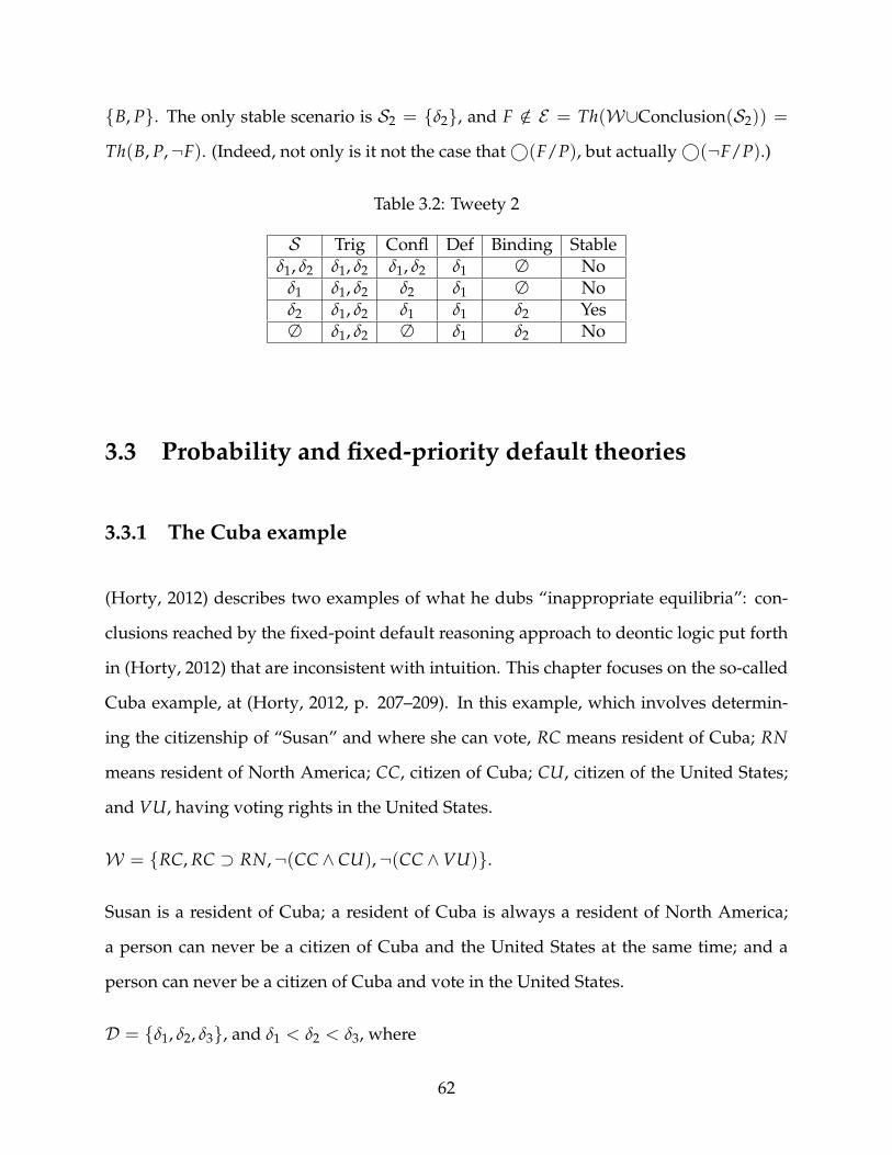
{B, P}. The only stable scenario is S2 = {δ2}, and F /∈ E = Th(W∪Conclusion(S2)) =

Th(B, P,¬F). (Indeed, not only is it not the case that©(F/P), but actually©(¬F/P).)

Table 3.2: Tweety 2

S Trig Confl Def Binding Stableδ1, δ2 δ1, δ2 δ1, δ2 δ1 ∅ No

δ1 δ1, δ2 δ2 δ1 ∅ Noδ2 δ1, δ2 δ1 δ1 δ2 Yes∅ δ1, δ2 ∅ δ1 δ2 No

3.3 Probability and fixed-priority default theories

3.3.1 The Cuba example

(Horty, 2012) describes two examples of what he dubs “inappropriate equilibria”: con-

clusions reached by the fixed-point default reasoning approach to deontic logic put forth

in (Horty, 2012) that are inconsistent with intuition. This chapter focuses on the so-called

Cuba example, at (Horty, 2012, p. 207–209). In this example, which involves determin-

ing the citizenship of “Susan” and where she can vote, RC means resident of Cuba; RN

means resident of North America; CC, citizen of Cuba; CU, citizen of the United States;

and VU, having voting rights in the United States.

W = {RC, RC ⊃ RN,¬(CC ∧ CU),¬(CC ∧VU)}.

Susan is a resident of Cuba; a resident of Cuba is always a resident of North America;

a person can never be a citizen of Cuba and the United States at the same time; and a

person can never be a citizen of Cuba and vote in the United States.

D = {δ1, δ2, δ3}, and δ1 < δ2 < δ3, where

62

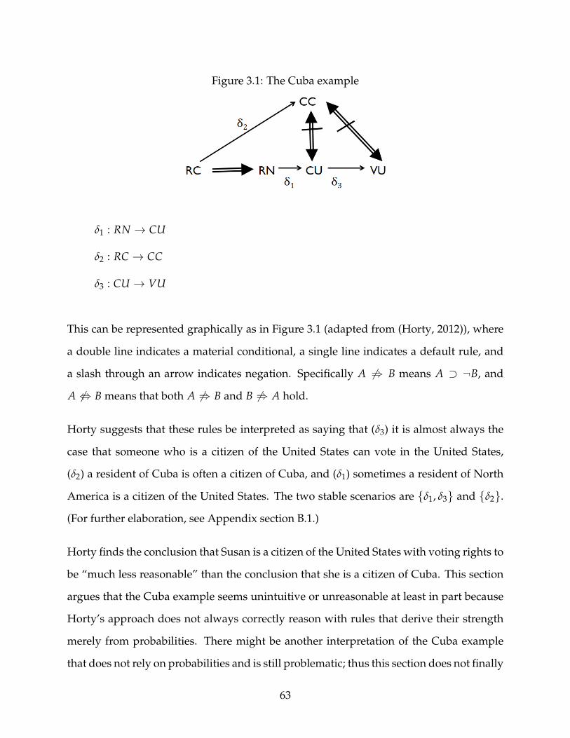
Figure 3.1: The Cuba example

δ1 : RN → CU

δ2 : RC → CC

δ3 : CU → VU

This can be represented graphically as in Figure 3.1 (adapted from (Horty, 2012)), where

a double line indicates a material conditional, a single line indicates a default rule, and

a slash through an arrow indicates negation. Specifically A 6⇒ B means A ⊃ ¬B, and

A 6⇔ B means that both A 6⇒ B and B 6⇒ A hold.

Horty suggests that these rules be interpreted as saying that (δ3) it is almost always the

case that someone who is a citizen of the United States can vote in the United States,

(δ2) a resident of Cuba is often a citizen of Cuba, and (δ1) sometimes a resident of North

America is a citizen of the United States. The two stable scenarios are {δ1, δ3} and {δ2}.

(For further elaboration, see Appendix section B.1.)

Horty finds the conclusion that Susan is a citizen of the United States with voting rights to

be “much less reasonable” than the conclusion that she is a citizen of Cuba. This section

argues that the Cuba example seems unintuitive or unreasonable at least in part because

Horty’s approach does not always correctly reason with rules that derive their strength

merely from probabilities. There might be another interpretation of the Cuba example

that does not rely on probabilities and is still problematic; thus this section does not finally

63

resolve the question of the Cuba example. Rather, it uses the Cuba example to highlight

the problem for (Horty, 2012) with probabilities.

3.3.2 Probabilities

The problematic stable scenario of the Cuba example can be traced at least in part to the

interaction of RC ⊃ RN and δ1 : RN → CU, and the fact that Horty’s approach does not

necessarily provide results consistent with a probabilistic analysis.

Consider the following {W , ∆,<} fixed-priority default theory without any interpreta-

tion.

W = {RC}

δ0 : RC → CU

The stable scenario is {δ0}, for the single rule is triggered, is not defeated, and is not

conflicted. Formally, this is correct. Read this default rule δ0 as: “If something is RC, then

barring information to the contrary, assume that the thing is CU.”

Now assume that RC means that a person is a resident of Cuba and CU means that a

person is a citizen of the United States. The default rule δ0 now states, “If a person is a

resident of Cuba, then barring information to the contrary, assume that the person is a

citizen of the United States.”

With this interpretation, RC → CU is not a good default rule. A default rule is supposed

to be true in general, or true barring information to the contrary. In fact, while there are

some citizens of the United States who live in Cuba, the vast majority of people who are

residents of Cuba are not citizens of the United States.

64

The natural next step is to consider high-probability rules only. But high probability is

not sufficient to establish a default rule. As this section will show, we should reject the

following proposed rule (PR):

(PR) If, given X, the chance of Y is greater than 50%, then X → Y is a default

rule.

Consider {W , ∆,<}:

W = {RC, RC ⊃ RN}

δ1 : RN → CU

The stable scenario is {δ1}, for the rule is triggered, is not defeated, and is not conflicted.

There is nothing wrong with this formalization. The material conditional can be read as

“If something is RC, then that thing is definitely RN,” and the default rule as “If some-

thing is RN, then barring information to the contrary, assume that the thing is CU.”

With certain interpretations, however, this reasoning goes awry. Interpret the theory as

follows: RN means that a person is a resident of North America, RC means that a person

is a reside of Cuba, and CU means that a person is a citizen of the United States. It is al-

ways true that if a person is a resident of Cuba, that person is a resident of North America.

That is a fact about geography. This is not a default rule; it is a material conditional. And

it is in fact more likely than not that, given that a person is a resident of North America,

that person is a citizen of the United States.2 If (PR) is correct, δ1 is a satisfactory default

rule.2Roughly 65% to 70% of residents of North America are U.S. citizens. About 57% of the approximately

528.7 million residents of North America are residents of the United States, and 97% of United States resi-dents are United States citizens (Central Intelligence Agency, 2014). Additionally, at least 3.7 million UnitedStates citizens live outside the United States but in North America (Central Intelligence Agency, 2014).

65

Figure 3.2: Base Rates: Cuban Resident, U.S. Citizen (not to scale)

But this interpretation leads to the following conclusion: Given that a person is a resident

of Cuba, barring information to the contrary, conclude that the person is a citizen of the

United States. What has gone wrong?

The problem is that although δ1 itself is a high-probability rule, a very low-probability

implication has snuck into the analysis. If RN → CU is a default rule only because it

captures something about probabilities, it is clearly flawed reasoning to combine that with

RC ⊃ RN and conclude that RC → CU. For one cannot conclude from P(RN|RC) = 1

and P(CU|RN) > 50% that P(CU|RC) > 50%. To put this in terms of argumentation: the

argument “all X are Y, and a majority of Y are Z, so a majority of X are Z” is not a good

argument. (This is represented graphically in Figure 3.2.) So reject (PR). It’s not that a rule

isn’t ever a default rule if the probability of X given Y is greater than 50%. But probability

greater than 50% isn’t sufficient to qualify something as a default rule.

These rules are embedded in the Cuba example (highlighted in Figure 3.3), and are at least

partially responsible for the unintuitive stable scenario, under the interpretation provided

in (Horty, 2012). Again, the stable scenario seems wrong here because the outcome is

contrary to something we know to be true based on facts in the world: we know that the

probability that a person is a citizen of the United States, given that the person is a resident

of Cuba, is low. As the Appendix shows, however, the Cuba example is equivalent to

a simpler example that is plainly structurally problematic. Just as Chapter 4 does not

66

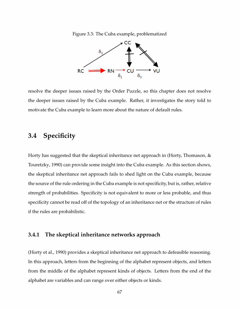
Figure 3.3: The Cuba example, problematized

resolve the deeper issues raised by the Order Puzzle, so this chapter does not resolve

the deeper issues raised by the Cuba example. Rather, it investigates the story told to

motivate the Cuba example to learn more about the nature of default rules.

3.4 Specificity

Horty has suggested that the skeptical inheritance net approach in (Horty, Thomason, &

Touretzky, 1990) can provide some insight into the Cuba example. As this section shows,

the skeptical inheritance net approach fails to shed light on the Cuba example, because

the source of the rule ordering in the Cuba example is not specificity, but is, rather, relative

strength of probabilities. Specificity is not equivalent to more or less probable, and thus

specificity cannot be read off of the topology of an inheritance net or the structure of rules

if the rules are probabilistic.

3.4.1 The skeptical inheritance networks approach

(Horty et al., 1990) provides a skeptical inheritance net approach to defeasible reasoning.

In this approach, letters from the beginning of the alphabet represent objects, and letters

from the middle of the alphabet represent kinds of objects. Letters from the end of the

alphabet are variables and can range over either objects or kinds.

67

An assertion has the form x → y (a positive assertion) or x 6→ y (a negative assertion). y is

a kind, while x may be either an object or a kind. If x is an object, then the assertion is an

atomic statement. To use the classic nonmonotonic example, where a represents Tweety,

and p represents bird, a→ p means “Tweety is a bird,” and is equivalent to, for example,

Pa, where P is the predicate “is a bird.”

If x is a kind, then the assertion does not have an equivalent in standard logic. Where p

indicates “bird” and q ”flies,” then p → q is interpreted as the generic statement “Birds

fly.” This isn’t the same as a universally quantified statement (e.g., ∀x(Px → Qx)), which

would mean, “for all a, if a is a bird, a can fly,” because this system is nonmonotonic. One

might read the generic statement as “in general, if x is a bird, then x can fly,” or “that x is

a bird tends to support the conclusion that x can fly.” p 6→ q can be read as “In general,

birds don’t fly.” So p 6→ q is something like p→ ¬q.

Capital Greek letters represent networks, also called nets. A network is a set of individ-

uals (I), a set of kinds (K), a set of positive links, and a set of negative links. The sets of

links are finite subsets of (I×K)∪ (K×K). That is, a link could be of the form a→ p (the

“Tweety is a bird” atomic statement example); a 6→ p; p→ q (“Birds fly”); or p 6→ q.

A lowercase Greek letter ranges over sequences of links. One particular type of sequence

of links is a path, which can be defined inductively:

1. Every assertion is a path.

2. If σ→ p is a path, then σ→ p→ q is a path.

3. If σ→ p is a path, then σ→ p 6→ q is a path.

A negative link can thus occur only as the final link of a path, and an individual can be

the first node of a path only.

68

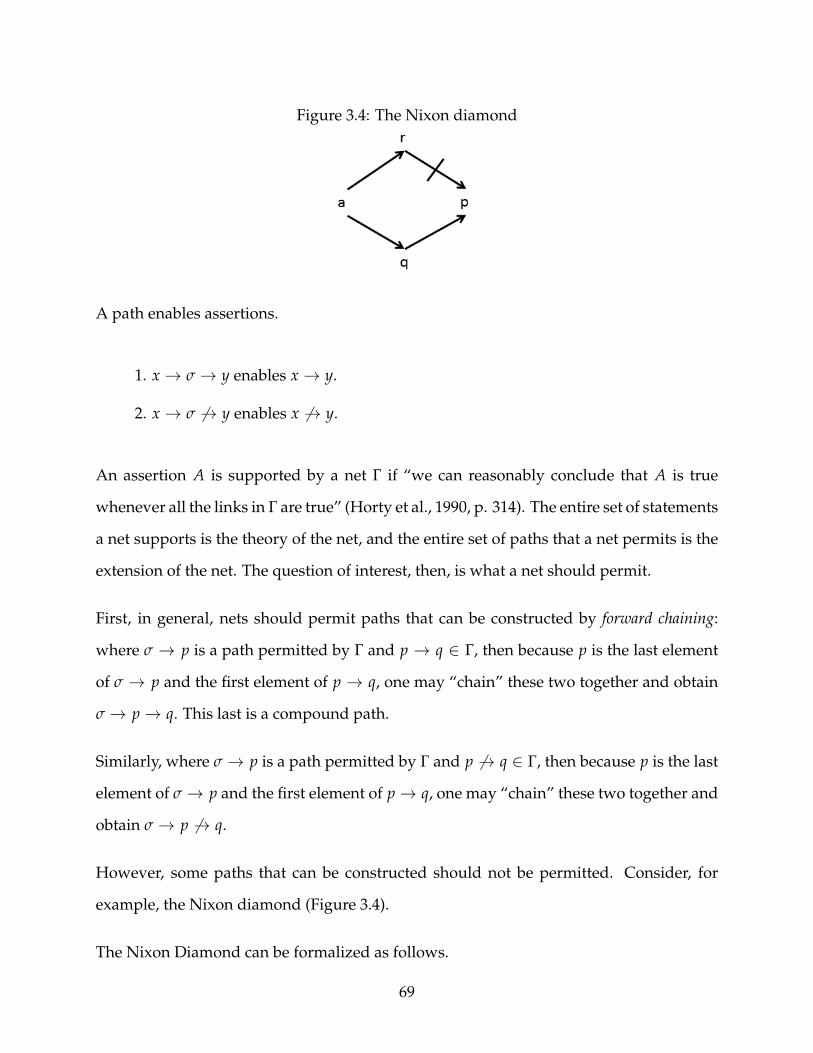
Figure 3.4: The Nixon diamond

A path enables assertions.

1. x → σ→ y enables x → y.

2. x → σ 6→ y enables x 6→ y.

An assertion A is supported by a net Γ if “we can reasonably conclude that A is true

whenever all the links in Γ are true” (Horty et al., 1990, p. 314). The entire set of statements

a net supports is the theory of the net, and the entire set of paths that a net permits is the

extension of the net. The question of interest, then, is what a net should permit.

First, in general, nets should permit paths that can be constructed by forward chaining:

where σ → p is a path permitted by Γ and p → q ∈ Γ, then because p is the last element

of σ → p and the first element of p → q, one may “chain” these two together and obtain

σ→ p→ q. This last is a compound path.

Similarly, where σ→ p is a path permitted by Γ and p 6→ q ∈ Γ, then because p is the last

element of σ→ p and the first element of p→ q, one may “chain” these two together and

obtain σ→ p 6→ q.

However, some paths that can be constructed should not be permitted. Consider, for

example, the Nixon diamond (Figure 3.4).

The Nixon Diamond can be formalized as follows.

69

I = {a}

K = {p, q, r}

Lp = {a→ r, a→ q, q→ p}

Ln = {r 6→ p}

Following only the forward chaining approach, construct Path 1, a → r 6→ p, and thus

enable a 6→ p, but also construct Path 2, a → q → p, and thus enable a → p. One might

conclude that either Path 1 or Path 2 is permissible. (Horty et al., 1990) takes a different,

skeptical approach, and conclude that the two paths neutralize each other—that neither

should be accepted.

(Horty et al., 1990) places two restrictions on neutralization: (1) only compound paths

may be neutralized, and (2) a path may be neutralized only by paths which are not them-

selves preempted. I explain the meaning of and reasoning behind each of these restric-

tions in turn.

First, only compound paths may be neutralized because one must be able to conclude

from a set of information everything contained in that set. For example, if one considers

Γ where

Lp = {a→ r}

Ln = {a 6→ r}

one wants to be able to conclude both a → r and a 6→ r, because the underlying set itself

is inconsistent.

Second, a path that is preempted (as defined shortly) cannot neutralize another path.

Consider the following net:

70

I = {a}

K = {p, q, r}

Lp = {a→ p, p→ q, q→ r}

Ln = {p 6→ r}

To stimulate intuition, this can be considered the Tweety fact pattern, where a is Tweety,

p is Penguins, q is Birds, and r is Flying Things. Should one conclude that Tweety can

fly? One can construct Path 1, a → p → q → r, i.e., Tweety is a flying thing. But one can

also construct Path 2, a → p 6→ r. Horty prefers Path 2, as it is drawn from more specific

information (about penguins) as opposed to general information (about birds).

Thus one defines preemption as follows:

x → τ → υ → y is preempted in a net Γ exactly when there is some node

z such that z 6→ y ∈ Γ, and either z = x or Γ permits a path of the form

x → τ1 → z→ τ2 → υ.

Similarly,

x → τ → υ 6→ y is preempted in a net Γ exactly when there is some node

z such that z → y ∈ Γ, and either z = x or Γ permits a path of the form

x → τ1 → z→ τ2 → υ.

Applying this definition to the example of Tweety, a→ p→ q→ r is preempted because

there is a node, p, such that p 6→ r ∈ Γ, and the net permits a → p → q. Intuitively,

a→ p→ q tells us that p is more specific than q, and p 6→ r tells us that this more specific

information contradicts the information arrived at from q.

71

Now we are almost in a position to define inheritance formally. Let |. be the permission

relation. Γ |. σ means that Γ permits the path σ. To define |. inductively, one must have

some concept of “less than” for two paths, as to make the argument inductively that Γ |. σ,

one must be able to make the statement that Γ |. σ′ for every σ′ ”less than” (in some sense)

σ in Γ.

(Horty et al., 1990) points out that identifying complexity with length does not work. For

example, consider

K = {p, q, r}

Lp = {x → p, p→ y, x → q, q→ r}

Ln = {r 6→ y}

We can create Path 1 = x → p→ y, but we can also create Path 2 = x → q→ r 6→ y.

Path 1 and Path 2 conflict, because from Path 1 we can assert x → y, and from Path 2 we

can assert x 6→ y. Thus Path 1 should not be permitted, because it is not a direct path,

and it conflicts with a nonpreempted path. Here, we cannot know to reject Path 1 until

we have considered a longer path, Path 2.

Somehow, one must find a method to check all relevant paths before one can conclude

that a particular path is to be accepted or is, to the contrary, neutralized. Checking all

shorter paths isn’t sufficient. To resolve this problem, Horty et al. introduce the idea of

complexity.

First, consider a generalized path, which is like an ordinary path—a series of links—but

unlike an ordinary path, which contains a negative link ( 6→) if at all only as the last link,

a generalized path can contain a negative link anywhere, and any number of negative

links. (If σ is a generalized path, so is σ→ y and σ 6→ y.)

72

The degree of a path σ, degΓ(σ), is the length of the longest generalized path in the net

from the initial node of the path to its end node.

Now one can define |. , permission. It is a definition by cases and induction.

Case 1: σ is a direct link (i.e., it is not a compound path). Then Γ |. σ iff σ ∈ Γ.

Case 2: σ is a compound path with degΓ(σ) = n. Assume, for purposes of induction, that

it is known whether Γ |. σ′ for all σ′ such that degΓ(σ′) < n. Consider the two possible

cases:

1. σ is a positive path, of the form x → σ1 → u→ y. Then Γ |. σ iff all of the following are

true:

(a) Γ |. x → σ1 → u.

(b) u→ y ∈ Γ.

(c) x 6→ y /∈ Γ.

(d) For all υ, τ such that Γ |. x → τ → υ, where υ 6→ y ∈ Γ, there exist z, τ1, τ2

such that z → y ∈ Γ and either z = x or there exist τ1, τ2 with Γ |. x → τ1 →

z→ τ2 → υ.

2. σ is a negative path, of the form x → σ1 → u 6→ y. Then Γ |. σ iff all of the following

are true:

(a) Γ |. x → σ1 → u.

(b) u 6→ y ∈ Γ.

(c) x → y /∈ Γ.

73

(d) for all υ, τ such that Γ |. x → τ → υ, where υ 6→ y ∈ Γ, there exist z, τ1, τ2

such that z 6→ y ∈ Γ and either z = x or there exist τ1, τ2 with Γ |. x → τ1 →

z→ τ2 → υ.

(a) and (b), in each case, formalize “forward chaining”: adding links to paths based on

links that already exist in Γ. (d) permits paths to be created only if potentially conflicting

paths are preempted. And (c) bars paths that conflict with direct links.

3.4.2 The technical claim: Order of application

Horty makes two claims about the skeptical inheritance approach and the Cuba example.

First, he states that the “correct” answer (i.e., the single intuitively acceptable scenario)

is reached “when [the] defaults [in the Cuba example] are considered in order of their

degree” (Horty, 2012, p. 209, n. 7). This is a technical claim. And, second, “the intuitions

underlying. . . [(Horty et al., 1990)]. . . would. . . tell us that [Susan] is a citizen of Cuba, not

a citizen of the US, and that [s]he does not have voting rights in the US” (Horty, 2001, p.

13). While this claim involves understanding the technical program put forth in (Horty,

2001), it is ultimately a claim about intuitions, not a technical claim. I consider each claim

in turn.

The skeptical inheritance approach cannot directly model the Cuba example. The skepti-

cal inheritance approach can be used only when all rules are defeasible, whereas the Cuba

example includes both strict and defeasible rules. For example, it is a strict rule that if one

is a resident of Cuba, one is a resident of North America (RC ⊃ RN), but it is a defeasible

rule that in general, if one is a resident of Cuba, one is a citizen of Cuba (RC → CC).

Horty does not in fact suggest applying the skeptical inheritance approach to the Cuba

example: rather, he proposes using an order-of-application approach to analyze the Cuba

74

example, where the order of application is from lowest to highest degree.

However, a technical problem remains. Degrees are available only for acyclic nets

(Horty et al., 1990, p. 322). This makes sense, because the degree of a path is the longest

possible generalized path between two nodes; if the net is cyclic, degree is not well-

defined. The Cuba example, however, is cyclic, because it includes ¬(CC ∧ CU) and

¬(CC ∧VU) (that is, it includes CC 6⇔ CU and CC 6⇔ VU) (see Figure 3.1).

Thus consider a simplified version of the Cuba example to flesh out Horty’s claim that

order-of-application, with degrees as the ordering, gives the “correct” result. Assume

that all rules are defeasible, and modify the net so that it is acyclic. Where a is Susan,

and CC, CU, VU, RN, RC are kinds, reflecting the problem as sketched above, the net is

formalized as follows and appears as in Figure 3.5.

I = {a}

K = {CC, CU, VU, RN, RC}

Lp = {a→ RC, RC → RN, RN → CU, CU → VU}

Ln = {CC 6→ CU, CC 6→ VU}

Figure 3.5: The modified Cuba example

With this modification, the degrees of various paths are as follows:

75

Degree 1: All direct links that are the longest generalized path between two

nodes.

Degree 2: a→ RN, a→ CC

Degree 3: a→ CU

Degree 4: a→ VU

Now apply these rules in the order of degree. Horty does not indicate exactly how to do

this; here I apply, informally, essentially the approach of (Brewka & Eiter, 2000).

First accept each direct link of degree 1 that is the longest generalized path between two

nodes. Accept that Susan is a resident of Cuba; that if she is a citizen of Cuba, she is not a

citizen of the United States; and if she is a citizen of Cuba, she does not vote in the United

States.

Then apply rules of Degree 2, and accept that Susan is a resident of North America and a

citizen of Cuba. Because we have already accepted that if she is a citizen of Cuba, she is

not a citizen of the United States, also accept that she is not a citizen of the United States.

Now apply rules of Degree 3. Do not accept a→ CU, because this conflicts with a propo-

sition already accepted—that she is not a citizen of the United States.

Finally, apply rules of Degree 4. Do not accept that she votes in the United States, because

this conflicts with ¬VU, which is accepted due to a combination of rules of Degree 1 and

rules of Degree 2.

Thus arrive at the putative single correct answer: Susan is a resident and citizen of Cuba,

who votes in Cuba. The scenario in which Susan is a resident of Cuba and a citizen of the

United States who votes in the United States is not possible, because the rules that would

support that scenario are conflicted out by lower-degree rules.

76

While this is the desired result, the “correct” answer does not come from applying the

actual skeptical inheritance approach to the actual Cuba example, or even to the modi-

fied Cuba example. Thus Horty’s reason for suggesting, at (Horty, 2001, p. 13), that the

skeptical inheritance net approach guides us toward the single correct answer must be an

intuitive one, not a technical one, and it is to that intuitive claim that I now turn.

3.4.3 The intuitive claim: What is specificity?

Horty criticizes the approach of (Prakken & Sartor, 1998) to defeasible reasoning based

in part on the result that approach provides in the Cuba example. Of particular interest

for purposes of this chapter, Horty claims that the “intuitions underlying the skeptical

inheritance theory” suggest a different result than (Prakken & Sartor, 1998). To under-

stand this claim, we must first understand Horty’s description of the approach proposed

in (Prakken & Sartor, 1998).

As (Horty, 2001) describes a slightly simplified version of (Prakken & Sartor, 1998), con-

sider a language where a literal is an atomic formula or a negated atomic formula, either

A or ¬A. Where Li is a literal, literals can be combined into rules, which are either strict

rules or defeasible rules. A strict rule is written as Lj ⇒ Lk, and a defeasible rule is writ-

ten as Lj → Lk. Where L is an atomic formula A, L = ¬A, and if L is a negated atomic

formula ¬A, L = A.

An ordered theory, Γ, is a triple 〈S, D,<〉, where S is a set of strict rules, D is a set of

defeasible rules, and < is a partial ordering representing priority on the defeasible rules.

A rule with higher priority dominates a rule with lower priority.

An argument based on Γ is a finite sequence, α = [r0, . . . , rn] of rules from S ∪ D. The an-

tecedent of r0 must be>. The antecedent of ri+1 equals the consequent of ri. No two rules

77

in α may have the same consequent. ArgΓ is the set of arguments that can be constructed

from Γ.

α + σ is the concatenation of an argument, α, and a sequence, σ. A sequence of rules σ is a

strict sequence if it contains only strict rules. Two arguments based on the same Γ conflict

with each other exactly when there are strict sequences σ and σ′, and complementary

literals L and L, such that α + σ is an argument of Γ with conclusion L, and α′ + σ′ is an

argument of Γ with conclusion L. A “strict argument” is an argument that contains only

strict rules, and a defeasible argument is an argument that is not strict.

Finally, to capture the idea of the strength of an argument, assume that all strict arguments

are equally strong, all strict arguments are stronger than any defeasible argument, and the

strength of a defeasible argument is determined by the strength of the final defeasible rule

supporting that conclusion. Formally, let RL(α) represent the strength of an argument α,

where the argument has conclusion L. If the subargument of α up to L is strict (i.e.,

contains only strict rules), then RL(α) = ∞. Otherwise, RL(α) equals the last defeasible

rule in α that either contains L as its consequent, or is entirely prior to L.

Say that α defeats α′ when α and α′ conflict, and α is not weaker than α′. That is, α

defeats α′ when α and α conflict, i.e., there are strict sequences σ and σ′ such that α + σ

is an argument of Γ and has the conclusion L and α + σ′ is an argument of Γ and has

the conclusion L (this is the idea of conflict), and it is not the case that RL(α + σ) <

RL(α′ + σ′). If α defeats α′, but α′ does not defeat α, then α strictly defeats α′.

It’s not the case than an argument is acceptable exactly when it is not defeated. Rather, a

defeated argument may be acceptable if the argument that has defeated it is subsequently

defeated. This is the idea of reinstatement. Where Γ is an ordered theory, and S is a

subset of ArgΓ, α is acceptable with respect to S when each argument that defeats α is

itself defeated by some other argument belonging to S .

78

Define the characteristic function of Γ, FΓ, where for each subset S of ArgΓ:

FΓ(S) = {α ∈ ArgΓ : α is acceptable with respect to S}.

The set of justified arguments with respect to Γ is, by definition, the least fixed point of

FΓ, which always exists (Horty, 2001, p. 8).

Now apply this to the Cuba example.

Γ = 〈S, D,<〉

S = {> ⇒ RC, RC ⇒ RN, CC 6⇒ CU, CC 6⇒ VU}

(Recall: A 6⇒ B means A⇒ ¬B.)

Where

r1 = RN → CU

r2 = RC → CC

r3 = CU → VU

Then

D = {r1, r2, r3}

<:

r1 < r2

r2 < r3

and therefore r1 < r3

79

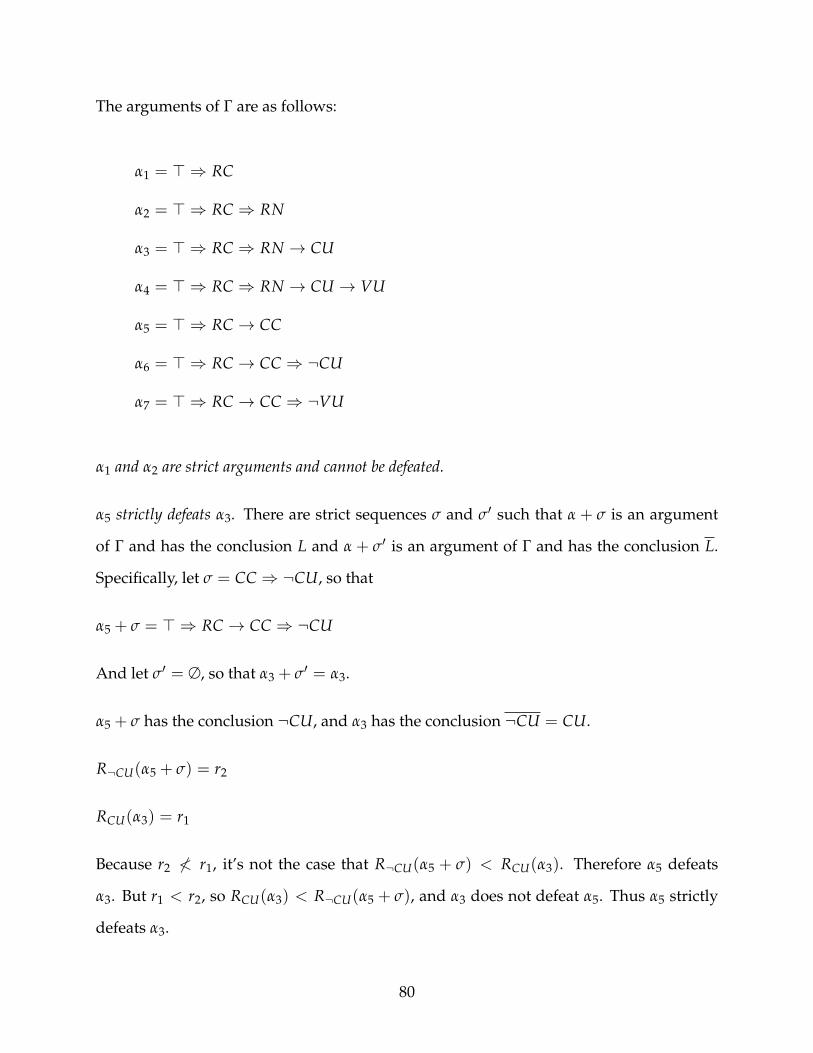
The arguments of Γ are as follows:

α1 = > ⇒ RC

α2 = > ⇒ RC ⇒ RN

α3 = > ⇒ RC ⇒ RN → CU

α4 = > ⇒ RC ⇒ RN → CU → VU

α5 = > ⇒ RC → CC

α6 = > ⇒ RC → CC ⇒ ¬CU

α7 = > ⇒ RC → CC ⇒ ¬VU

α1 and α2 are strict arguments and cannot be defeated.

α5 strictly defeats α3. There are strict sequences σ and σ′ such that α + σ is an argument

of Γ and has the conclusion L and α + σ′ is an argument of Γ and has the conclusion L.

Specifically, let σ = CC ⇒ ¬CU, so that

α5 + σ = > ⇒ RC → CC ⇒ ¬CU

And let σ′ = ∅, so that α3 + σ′ = α3.

α5 + σ has the conclusion ¬CU, and α3 has the conclusion ¬CU = CU.

R¬CU(α5 + σ) = r2

RCU(α3) = r1

Because r2 6< r1, it’s not the case that R¬CU(α5 + σ) < RCU(α3). Therefore α5 defeats

α3. But r1 < r2, so RCU(α3) < R¬CU(α5 + σ), and α3 does not defeat α5. Thus α5 strictly

defeats α3.

80

α5 defeats α4. Similar reasoning shows that α5 defeats α4. There are strict sequences σ

and σ′ such that α5 + σ is an argument of Γ and has the conclusion L and α4 + σ′ is an

argument of Γ and has the conclusion L.

Specifically, let σ = CC ⇒ ¬CU, so that

α5 + σ = > ⇒ RC → CC ⇒ ¬CU

And let σ′ = ∅, so that α4 + σ′ = α4.

α5 + σ has the conclusion ¬CU, and α4 contains3 ¬CU = CU.

R¬CU(α5 + σ) = r2

RCU(α4) = r1

Horty, as we will see, is intuitively comfortable with these results.

Additionally, however, the Argument System approach rejects α5, α7, and, according to

Horty, α6,4 none of which are justified. This is the portion that Horty rejects as unintuitive.

α4 defeats α5 and α7. Let σ = CC ⇒ ¬VU. α5 + σ is an argument in Γ—specifically,

α7. α7 supports the conclusion ¬VU. α4 supports the conclusion VU (so set σ′ = ∅).

R¬VU(α7) = r2. RVU(α4) = r3. Therefore α4 defeats α5, and α4 defeats α7.

According to Horty, through similar reasoning, α4 defeats α6. Thus one can conclude

3Horty explains this defeat by saying, “it is clear that α5 defeats α4, because α4 likewise supports [CU]through a default rule weaker than that through which [α6] supports ¬[CU]” (Horty, 2001, p. 13). Butwhile α4 supports CU, CU is not the conclusion of the argument α4. The definition of defeat allows thelengthening of arguments in certain circumstances to obtain a conclusion L, but does not appear to allowthe shortening of arguments to obtain a conclusion L (Horty, 2001, p. 6).

4I believe that the claim that α6 is not justified is an error on his part. An argument that defeated α6would have to have the conclusion CU. The only argument with this conclusion is α3, and RCU(α3) = r1,and R¬CU(α6) = r2. Horty’s claims do not depend on this, however. There is a typo on p. 13 of the Hortywhich may explain the error, as he writes “it is clear that α5 defeats α4, because α4 likewise supports [CU]through a default rule weaker than that through α7 supports ¬[CU].” But α7 does not contain CU—rather,α6 does.

81

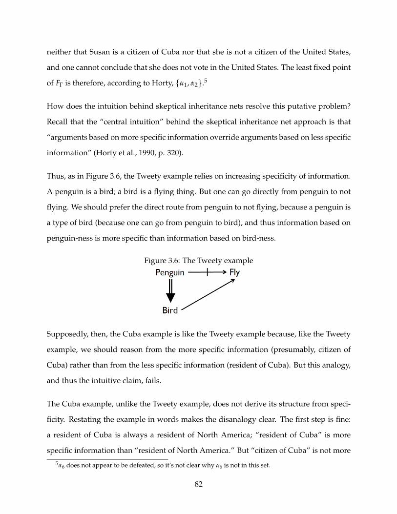
neither that Susan is a citizen of Cuba nor that she is not a citizen of the United States,

and one cannot conclude that she does not vote in the United States. The least fixed point

of FΓ is therefore, according to Horty, {α1, α2}.5

How does the intuition behind skeptical inheritance nets resolve this putative problem?

Recall that the “central intuition” behind the skeptical inheritance net approach is that

“arguments based on more specific information override arguments based on less specific

information” (Horty et al., 1990, p. 320).

Thus, as in Figure 3.6, the Tweety example relies on increasing specificity of information.

A penguin is a bird; a bird is a flying thing. But one can go directly from penguin to not

flying. We should prefer the direct route from penguin to not flying, because a penguin is

a type of bird (because one can go from penguin to bird), and thus information based on

penguin-ness is more specific than information based on bird-ness.

Figure 3.6: The Tweety example

Supposedly, then, the Cuba example is like the Tweety example because, like the Tweety

example, we should reason from the more specific information (presumably, citizen of

Cuba) rather than from the less specific information (resident of Cuba). But this analogy,

and thus the intuitive claim, fails.

The Cuba example, unlike the Tweety example, does not derive its structure from speci-

ficity. Restating the example in words makes the disanalogy clear. The first step is fine:

a resident of Cuba is always a resident of North America; “resident of Cuba” is more

specific information than “resident of North America.” But “citizen of Cuba” is not more

5α6 does not appear to be defeated, so it’s not clear why α6 is not in this set.

82

specific information than “resident of Cuba,” and “resident of North America” is not

more specific information than “citizen of the United States.” Rather, one way to classify

residents of Cuba is by their citizenship. Another way might be by their gender. But even

if, to make up an example, 60% of residents of Cuba were men, although we might say

that in general, if one is a resident of Cuba, one is a male (i.e., one can go from resident

of Cuba to male), we wouldn’t think that “resident of Cuba” is more specific information

than “male.”

What does “specific” mean? According to (Horty et al., 1990, p. 320), “the reason p can

be said to provide more specific information about a than q does is simply that the net

permits the path from a through p to q; this path, a → p → q, tells us both that Tweety is a

penguin and that a penguin is a specific type of bird.” But while that particular rule is an

example of specificity, specificity cannot in general be read off the topology of a net (or by

checking to see whether a path goes “through” a particular node). Specificity must mean

more than just that a rule can be stated that has one category on the lefthand side, and

here’s why:

Consider, for example, a population of 100 people, 60 male and 40 female. Of the 60 men,

36 have red hair and 24 have brown hair. Of the 40 women, 24 have red hair and 16 have

brown hair, as in Table 3.3.

Table 3.3: Probability example: groupsRed Hair Brown Hair Total

Men 36 24 60Women 24 16 40

Total 60 40 100

If someone has red hair, then it’s more likely that the person is a man (because 36 of the

60 people who have red hair are men). So write

Red→Man

83

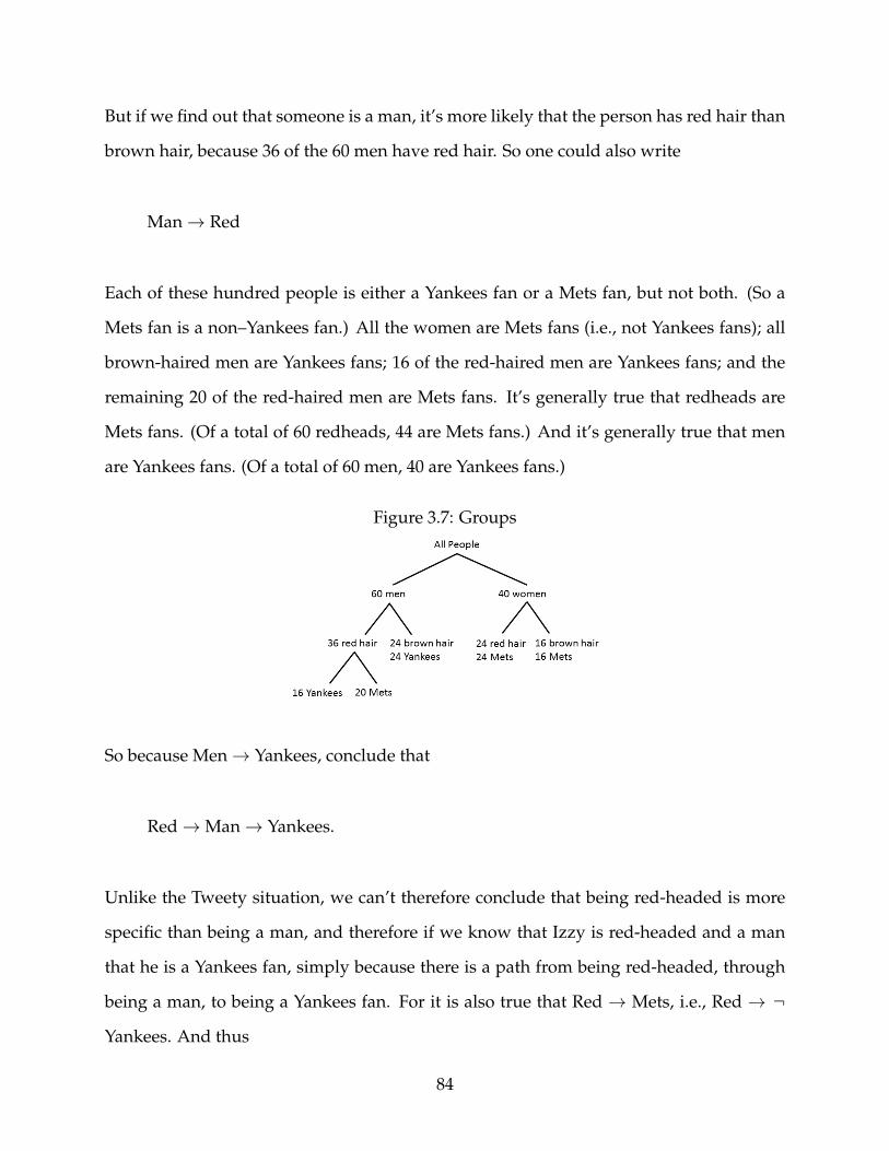
But if we find out that someone is a man, it’s more likely that the person has red hair than

brown hair, because 36 of the 60 men have red hair. So one could also write

Man→ Red

Each of these hundred people is either a Yankees fan or a Mets fan, but not both. (So a

Mets fan is a non–Yankees fan.) All the women are Mets fans (i.e., not Yankees fans); all

brown-haired men are Yankees fans; 16 of the red-haired men are Yankees fans; and the

remaining 20 of the red-haired men are Mets fans. It’s generally true that redheads are

Mets fans. (Of a total of 60 redheads, 44 are Mets fans.) And it’s generally true that men

are Yankees fans. (Of a total of 60 men, 40 are Yankees fans.)

Figure 3.7: Groups

So because Men→ Yankees, conclude that

Red→Man→ Yankees.

Unlike the Tweety situation, we can’t therefore conclude that being red-headed is more

specific than being a man, and therefore if we know that Izzy is red-headed and a man

that he is a Yankees fan, simply because there is a path from being red-headed, through

being a man, to being a Yankees fan. For it is also true that Red → Mets, i.e., Red → ¬

Yankees. And thus

84

Man→ Red→ ¬ Yankees.

One possible distinction between the examples is that the relationship of specificity might

be a strict relation. While this isn’t reflected in (Horty et al., 1990), which does not dis-

tinguish strict and defeasible rules, it is one distinction between the example of the red-

headed men and the example of penguins. That penguins are birds is a strict rule; that

men are red-haired is not a strict rule. But if strictness helps separate rules about speci-

ficity from other rules, then neither can the Cuba example be about specificity, for neither

RN → CU nor RC → CC is a strict rule.

Perhaps, however, one cannot read specificity off the red-headed/male/baseball fan rules

because this is not the kind of relationship that can be represented by default rules. But

it is difficult to distinguish the red-headed/male/baseball relationship from the Cuba

example. In both examples, the rules depend entirely on frequency of occurrence of some

characteristic. Specificity thus cannot resolve the Cuba example.

3.5 Generics

Horty and others refer to defaults as “generic” statements. Perhaps default logic reasons

about generics—that something is a default rule precisely when it is a generic. Perhaps

the problem with the Cuba example is that it uses as its default rules statements that are

not generics. As this section will show, however, there is no settled theory of generics;

default logic does not reason correctly about some generics; and some default rules that

are core to the arguments presented in (Horty, 2012) are not generics. The literature on

generics therefore cannot resolve the questions raised by the Cuba example.

85

3.5.1 What are generics?

Generics are general statements, such as “birds fly” and “dogs bark” (e.g., (Liebesman,

2011), (Leslie, 2012)). Generics “express general claims about kinds and categories” (Leslie,

2012). This sounds much like the description of a default rule as a “generalization”; “[an]

important regularit[y] [that] hold[s] ‘for the most part’ ”; a “generic truth” (Horty, 2012,

p. 17).

Theories of genericity do not resolve the problem of what constitutes a default rule, in

part because there is no one theory of genericity. Indeed, the questions of the proper

characterization of the logical structure and semantics of generics are difficult—even “in-

tractab[le]” (Liebesman, 2011, pp. 3, 7–8). So attempting to resolve the question of default

rules by appealing to theories of genericity may do not more than move the problem from

one difficult area to another.

That said, even with no more than a sense of what constitutes a generic, as the follow-

ing subsections will show, generics are both over- and under-inclusive when it comes

to statements about which default logic correctly reasons. This subsection thus reviews

various theories of genericity to establish a base on which the following two subsections

will build. In particular, this subsection describes three theories of generics, and a fourth

theory that posits that genericity as a separate operator does not exist. To get a sense of

various theories of generics, this section considers whether

(R) Residents of North America are citizens of the United States

is a generic that is true. (R) expresses a generalization about individual members of the

kind “residents of North America.” (R) does not intuitively seem to be a true generic, and

indeed, it comes out false under any of the prominent approaches.

86

3.5.1.1 Probability

One approach to generics is the probabilistic approach, as in (Cohen, 1999). (Both (Leslie,

2012) and (Asher & Pelletier, 2012) show, convincingly, a range of problems with the ap-

proach and establish that (Cohen, 1999) does not accurately characterize various gener-

ics.) Roughly speaking, Cohen’s probabilistic approach holds that a generic “Ks are F” is

true either when (1) the probability that an arbitrary K is F is greater than 50%, or (2) the

probability that a K, as opposed to some other alternative, is F is greater than 50%. Po-

sition (1), the absolute reading, is self-explanatory—“Ravens are black” is a true generic

just in case the chance that a randomly selected raven is black. Position (2) is less obvious.

Take the generic “Dutch people speak English” (Cohen, 1999, p. 58). This is false under

the absolute reading—a majority of Dutch people (explains Cohen) do not speak English.

But as compared to the average person, a Dutch person is more likely to speak English,

and so the generic “Dutch people speak English” is true. Or consider “Lions have manes”

(Cohen, 1999, p. 59). If a majority of lions are female, then the absolute reading of “lions

have manes” is false. But lions are more likely to have manes than are alternative animals

(or alternative mammals), so the generic is true. That said, a randomly chosen resident

of North America is more likely to be a citizen of the United States than not, so (R) meets

this requirement under the absolute reading.

(Cohen, 1999) also imposes an additional requirement of homogeneity: the more-likely-

than-not condition must hold for all “salient partitions” of K (Cohen, 1999, p. 81ff). A

salient partition is, roughly speaking, a division of the kind that is somehow relevant.

A possible division of residents of North America is division by country, such that one

partition would be “residents of Mexico.” It is not true that most residents of Mexico are

citizens of the United States, so (R) is not a true generic on this account.

87

3.5.1.2 Modality

(Asher & Pelletier, 2012), building on (Pelletier & Asher, 1997), takes generics to be modal

quantifiers. Informally, “Ks are F” is a true generic under this account when ”Ks are F”

is true at normal worlds for Ks. If generics capture what is normal about a kind (the

“possible worlds” approach of generics), then whether (R) is a true generic depends on

one’s belief about what is normal about the kind “residents of North America” (Pelletier

& Asher, 1997). A jingoistic citizen of the United States might believe (R); most people

would not. There is nothing more or less normal about being a citizen of Canada than

being a citizen of the United States.

3.5.1.3 Psychology

Under the approach to generics of (Leslie, 2007), what one might dub a “psychologi-

cal” approach to generics, (R) also comes out false.6 Leslie suggests a four-part test for

whether a generic of the form “Ks are Fs” is true. The first requirement is that any coun-

terinstances must be negative: any counterinstances must not possess some “equally pos-

itive alternative property” (Leslie, 2007, p. 385). Once that condition is met, then one of

three conditions must also be met. The conditions proceed from requiring less to more

information. First, if the quality F is a characteristic of Ks—if it is a type of regularity for

K—then some Ks are F. For example, animals have certain “characteristic dimensions”—

they make typical noises, for example. If someone hears an elephant make a trumpeting

noise, one might then say, “Elephants are animals that make trumpeting noises” (Leslie,

2007, p. 384). One need not survey all elephants, or even many elephants.

6Leslie’s approach is not meant to be a semantics, but rather a description of how people use generics inthe world. It is thus a psychological approach—or, as Leslie herself characterizes it, generics are a windowinto “one of the most central questions in cognitive science,” which warrants “empirical study” (Leslie,2013, p. 22).

88

If F is not on a characteristic dimension, but it is particularly striking, then some Ks must

be F, and other must be “disposed to be F” (Leslie, 2007, 384–385). For example, it isn’t the

case that “carrying illness” is a characteristic dimension for animals. And it isn’t the case

that most, say, mosquitoes carry the West Nile Virus. But carrying the West Nile Virus

is a “striking[,] horrific or appalling” fact (Leslie, 2007, p. 384). Moreover, even those

mosquitoes that don’t carry the West Nile Virus are capable of carrying or disposed to

carry the virus. Thus, “Mosquitos carry the West Nile Virus” is a true generic according

to Leslie.

Finally, if F is not on a characteristic dimension and isn’t particularly striking, then a

majority of Ks need to be F in order for the generic to be true. (Leslie, 2007, p. 386).

(R) comes out false under according to Leslie’s definition, for it fails the first prong of her

test. If a resident of North America is not a citizen of the United States, that resident has

some other equally positive quality—that person is, almost certainly, a citizen of some

other country.

3.5.2 Some generics are not default rules

There are at least some generics about which default logic cannot reason accurately.

(Leslie, 2007) points out that certain types of inferences that go through under default

reasoning are clearly wrong for generics. Consider the default reasoning scheme with

which we are familiar. Birds fly; Tweety is a bird; therefore, barring information to the

contrary, concludes that Tweety flies. This is of the form (using Horty’s schema):

W = {B}

D = {δ1}

89

δ1 : B→ F

So conclude that Tweety flies.

But some true generics hold with respect to any one example with very low probability.

Thus the low probability problem described in Section 3.3 arises. Consider the generic

“Mosquitoes carry the West Nile virus.” Let B mean “Buzzy is a mosquito” and F mean

“carries the West Nile Virus.” The default reasoning schema authorizes us to conclude

that, all else equal, we should conclude that Buzzy carries the West Nile virus. This isn’t

accurate—less than 1% of mosquitoes carry the West Nile virus. But the statement is

nonetheless a generic (Leslie, 2007, p. 389). Thus it is not the case that default logic

reasons accurately about all generics. That X is a generic is not sufficient to establish that

X can be a default rule.

3.5.3 Some default rules are not generics

There are nongenerics about which default logic can reason accurately.

(Pelletier & Asher, 1997) propose that nonmonotonic logic is a way to understand the

semantics of generics. However, they reject default logic as a way to formalize generics,

because generics have truth conditions:7

[D]efault logic does not provide us with an acceptable formalization of generic

statements. Default rules are rules, and therefore are sound or unsound—

rather than sentences, which are either true or false. If we analyze charac-

terizing sentences [of generics] using default rules, these sentences would not7Moreover, (Pelletier & Asher, 1997) point out, generic statements can be nested, and default rules can-

not. “People who work late nights do not wake up early” is considered a nested generic, because, as(Pelletier & Asher, 1997) describe, “they attribute properties which involve genericity (as expressed hereby the “habitual” predicate wakes up early to kinds which are defined by means of characterizing properties(people who work late nights)” (Pelletier & Asher, 1997, p. 38).

90

have truth values, and their meanings could not be specified by an ordinary

semantic function. One consequence of being neither true nor false—not be-

ing in the language—is that characterizing sentences would therefore not “talk

about the world,” instead they would “talk about” which inferences to draw.

And this seems to us a strike against such an account.

(Pelletier & Asher, 1997, p. 37)

“Talk[ing] about which inferences to draw”—what one should believe or do—is exactly

what Horty wants default rules to do. The exact project of (Horty, 2012) is to use default

logic to reason deontically. To demand that all default rules be generics would be to reject

the central project of (Horty, 2012). For example, “If I have arranged to dine with Twin

1, then, all things considered, I ought to dine with Twin 1” is certainly not a generic—but

it is part of the central example Horty uses to introduce his deontic logic (Horty, 2012,

p. 71). Horty’s deontic approach requires that default rules prescribe which inferences to

draw, or which actions to take. Therefore, that X is a generic is not necessary to establish

that X can be a default rule.

3.6 Conclusion: Legal rules as default rules

Horty has suggested, and I argue in Chapter 2, that the default logic approach to deontic

reasoning, as described in (Horty, 2012), captures certain types of legal reasoning. As

we have seen, that a statement is a generic is neither necessary nor sufficient for that

statement to be a default rule. But legal rules are not generics, so this observation does

not threaten the application of default logic to the law. And that default logic does not

capture probabilistic reasoning does not present a problem for applying default logic to

legal reasoning either. Legal rules derive both their force and their defeasibility from

91

sources other than probability. Or, to put it another way: for certain kinds of legal rules

“if X then Y,” the answer to the question, “Why do we make the assertion ‘if X then Y’?”

is not “Because in the world, if something is X, it is more likely than not that it is also Y.”

And the answer to the question “Why should we accept legal rule 1, if X then Y, over legal

rule 2, if X then not Y?” is never, “Because in the real world, if something is X, it is more

likely that it is Y than that it is not Y.”

One naturally asks from where legal rules derive their force, and, relatedly, whether in

certain circumstances one ought to disregard even nonconflicted legal rules. The debates

on these questions are extensive and very much ongoing, and far outside the scope of

this chapter (generally, compare (Hart, 1961) and his followers, with (Dworkin, 1967), on

the one hand, and natural-law theorists, on the other). Nobody argues, however, that the

source of the strength of legal rules is in some way probabilistic or that legal rules must

be generics. Thus the limits described in this chapter do not affect the applicability of

(Horty, 2012) to rule-based legal reasoning.

92

Chapter 4

Statutes as supernormal rules

4.1 Introduction

This chapter refines Horty’s approach to legal reasoning. Horty does not distinguish

between reasoning from cases (common law reasoning) and reasoning from legislative

and administrative guidance (what I will call, for simplicity’s sake, statutory reasoning).

I agree with Horty that common law rules are often best represented by default rules

with premises—in other words, as rules that are triggered only if certain conditions are

met. I differ from Horty, however, in the appropriate representation of statutory rules.

The chapter argues that, contra Horty, statutory rules are best understood as premise-free

commands of conditionals, rather than conditional commands. That is, setting aside juris-

dictional concerns, statutes and regulations are best represented as supernormal default

rules. Various anomalous results Horty identifies may be avoided in the context of legal

reasoning if statutory rules are properly characterized as premise-free.

93

4.2 Interpreting statutory rules

A default rule may naturally be interpreted as a putative or potential command. I claim

that, once the question of jurisdiction is taken as settled (of which more in subsection 4.4.2

below), a default rule that is an interpretation of a statutory rule should be triggered in

any ∆. That is, statutory rules are best understood as prerequisite free, of the form> → q.

(Horty, 2012) already takes all rules to be normal. Thus I am arguing that statutory rules

in Horty’s approach should be taken to be supernormal, that is, a normal rule where the

only premise is >.

Horty raises the distinction between conditional commands and commands of condition-

als with regard to one of the puzzling default theories that he describes, as described

further in subsection 4.3.1. But this distinction is not central for him; in one example he

gives, he notes simply that it is ambiguous whether the δ in question should be consid-

ered a command of a conditional rather than a conditional command, and perhaps any

problem arises because of the “running together of two distinct ways of interpreting the

. . . command” (Horty, 2012, p. 206). But when it comes to statutory rules, I argue, there

is no ambiguity: once jurisdictional requirements are met, legislative and administrative

rules are best understood as always applying to everyone, whether or not the immediate

facts of a person’s situation trigger one particular rule. Thus all such rules should always

be taken to be triggered.

Informally, one should think of a law not as “if X, then the law says that you must Y,” but

rather “the law says that if X, then you must Y.” This is in some sense a question of scope,

but to make clear intended meaning we cannot use the © operator, for a given δ might

not be obligatory (if it is not in a proper scenario). Take the operator L to mean “the law

says”—that is, to mark out the scope of the putative (attempted) command. My claim is

that statutes are best interpreted as L(X ⊃ Y), and not as X → L(Y). The natural way to

94

make this change in Horty’s approach is to substitute ⊃ for→ in all δ and prepend > →

to what results.

Horty presents his theory as usefully applying in the context of statutory law. In this

example (slightly simplified in my retelling), in (Horty, 2012, Section 5.1.2), Smith has

loaned money to Miller for the purchase of a ship, and the ship serves as collateral for

the loan. Miller defaults on the loan as part of going bankrupt, and Smith is now trying

to determine whether his security interest in a ship has been perfected (“Per f ected”)–i.e.,

whether he can enforce his claim on the ship against the bankruptcy estate. But two

possible laws might apply: either the Uniform Commercial Code as enacted by the state

in which Miller, Smith, and the ship are located (the “UCC”) or the Ship Mortgage Act

(the “SMA”). The SMA is a federal statute, which tends to control over a state statute

(“Lex Superior”). But the UCC was enacted later than the SMA, and later statutes tend to

control over earlier statutes (“Lex Posterior”). Horty posits that Lex Posterior dominates

Lex Superior, so that the UCC dominates the SMA, i.e., δUCC > δSMA.

Possession means that Smith possesses the ship, and Documents means that Smith has

filed the correct documents. In this situation, Smith has possession of the ship but has

not filed the documents, so W = {Possession,¬Documents}. Finally, the UCC rule is

that an individual’s security interest in a ship is perfected if he has possession of the

relevant collateral (in this case, the ship); the SMA rule is that if an individual has not

filed the relevant documents, the individual’s security interest cannot be perfected. Horty

represents the relevant rules as δUCC : Possession→ Per f ected and δSMA : ¬Documents→

¬Per f ected.

My point is that we should take the UCC to say not, “If an individual has possession of

the relevant collateral, then the law is that the individual’s security interest is perfected,”

but rather, “The law is that if an individual has possession of the relevant collateral, then

the individual’s security interest is perfected.” The rule is binding whether or not the

95

person has possession of the relevant collateral. Similarly for the SMA rule. Thus the two

rules should be represented as δ′UCC : > → (Possession ⊃ Per f ected) and δ′SMA : > →

(¬Documents ⊃ ¬Per f ected).

In this particular example, the distinction between command of a conditional and con-

ditional command makes no difference. W includes both Possession and ¬Documents,

so both rules are triggered regardless of whether the rules are taken as commands of

conditionals or conditional commands. Thus, because δUCC > δSMA, Smith’s interest is

perfected.

But the distinction I have identified does matter. Horty identifies several puzzles that

arise from his approach to default logic and provides interpretations that either obviate

the puzzle (in the case of the Order Puzzle) or highlight the problematic nature of the

puzzle (in the case of inappropriate equilbria). These puzzles are a good entry to seeing

why it matters whether statutes and regulations are interpreted as supernormal.

4.3 Horty’s puzzles

4.3.1 The Order Puzzle

Horty describes a set of default rules that he calls the “Order Puzzle” (Horty, 2012, p.

201). In the Order Puzzle, there are three rules, δ1, δ2, and δ3, where δ3 dominates δ2,

and δ2 dominates δ1. The world of certain beliefs contains only W. The strongest rule,

δ3, is triggered only by the weakest rule, δ1. The middle rule is triggered by W, and its

conclusion contradicts the conclusion of the strongest rule.

That is:

96

W = {W}

δ1 < δ2 < δ3

δ1 : W → H

δ2 : W → ¬O

δ3 : H → O

Under Horty’s approach, the single stable scenario is {δ1, δ3}. (For an elaboration of the

reasoning behind this stable scenario, see Appendix section B.2.)

This example appears problematic if one takes an order-of-application approach to de-

fault reasoning. In such an approach, generally speaking, one adds to one’s belief set the

highest-remaining triggered rule that is consistent with rules in one’s belief set. Thus if

one follows, for example, (Brewka, 1994), which addresses this puzzle, one first adds δ2

to one’s belief set, because it is the highest-ranking rule that is triggered. Then one adds

δ1. Now δ3 is triggered, but too late, because δ3 is inconsistent with the two rules already

added to the belief set. So the unique correct belief set on the (Brewka, 1994) approach is

{δ1, δ2}. This seems odd, because {δ1, δ3} is also consistent, and, it would seem, preferable

to {δ1, δ2}, because δ3 is higher-ranked than δ2.

(Brewka & Eiter, 2000) resolves this problem by requiring the reasoner to delete any

rules that are, roughly speaking, defeated by higher-ranking rules, and ultimately ac-

cepts {δ1, δ3} as the single stable scenario. (Delgrande, Schaub, Tompits, & Wang, 2004,

p. 13) also describes this problematic collection of default rules and rejects it as having no

extension at all because it conflicts with the “normal order” of rule application.

Horty rejects the idea that this set of rules is incoherent by telling a story that he finds in-

tuitively attractive. Imagine, he says, that the rules are a set of commands given by three

97

officers. (That something is a command does not necessarily mean that the command is

part of a binding scenario and should actually be followed.) δ3 is higher priority than δ2

because it was given by a higher-ranking officer, and similarly for δ2 and δ1. The com-

mands may be strange, Horty states, but they are not impossible, and, he claims, it clearly

makes the most sense to obey {δ1, δ3} (Horty, 2012, p. 204). (Horty here appeals to the

reader’s intuition.)

Horty suggests that he finds his approach useful in the legal context. But one natural legal

interpretation of the Order Puzzle makes Horty’s story problematic. Consider the follow-

ing interpretation: all of the statements are about payments, and “W” means “is salary”;

“O” means “not deductible” (so ¬O means “deductible”); and “H” means “provides a

significant future benefit.” So δ3 means “If a payment is provides a significant future ben-

efit, then it is not deductible,” δ2 means “If a payment is salary, then it is deductible,” and

δ1 means “If a payment is salary, then it provides a significant future benefit.”

Additionally, say that δ3 is more persuasive than δ2 because δ3 is a rule from the Supreme

Court, and δ2 is a statute, and δ2 is more persuasive than δ1 because δ1 is a mere regulation.

(Ceteris paribus, Supreme Court rulings are more persuasive than statutes or regulations,

and statutes are more persuasive than regulations.) If one accepts S = {δ1, δ3}, the only

stable scenario, the salary payment would be treated as providing a significant future

benefit and as not deductible. To reach this result, one disregards a statute to make room

for a regulation. But the result that one would expect as a matter of legal analysis is that

the Supreme Court ruling and the statute would be respected, and thus that the belief set

S = {δ2, δ3} would be accepted. Under this story, the salary payment is not treated as

providing a significant future benefit and is deductible.

Or, to put an even finer point on it, imagine that Henry is deciding what position to

take on his tax return. δ3 is a statute, δ2 is a regulation, and δ1 is an instruction from

Henry’s lawyer. δ3 > δ2, because ceteris paribus, statutes are more persuasive than reg-

98

ulations. And δ2 > δ1, because regulations are more persuasive than a lawyer’s advice.

But a lawyer’s advice might still be taking as a (defeasible) rule to follow—the idea being

something like, “I will follow the instructions my lawyer gives me—after all, that is why

I pay him!—but the instructions he gives can always be defeated by actual law.” The sta-

ble scenario S = {δ1, δ3} suggests that Henry should follow the statute and his lawyer’s

instructions, but disregard the regulation. This clearly cannot be correct.

Horty’s story fails when the Order Puzzle is given these interpretations because, as ar-

gued in section 4.2, legal rules should be interpreted as supernormal—as commands of

conditionals—not as conditional commands.1

Horty writes that it is ambiguous whether δ3, in his example, should be considered a com-

mand of a conditional (i.e., apply δ′3 : > → (H ⊃ O)) rather than a conditional command

(i.e., δ3 : H → O). As Horty notes, if δ3 is read as a command of a conditional rather than

a conditional command, then the unique stable scenario is S = {δ2, δ′3} (Horty, 2012, p.

206). But in the legal context there is no ambiguity: the correct interpretation, if δ3 is a

statutory rule, is in fact δ′3. The Order Puzzle with Command of Conditional is thus as

follows:

W = {W}

δ1 < δ2 < δ3

1What I propose here does not resolve deeper problems that the Order Puzzle presents. As in (Hansen,2008, p. 250), one may present an epistemic version of the Order Puzzle that cannot, it seems, be properlyresolved by rewriting the various rules as supernormal. (Hansen, 2008, p. 263) argues that Horty’s appealto intuition is wrong for another reason:

[B]eing forced to violate a higher ranking order when obeying a lower ranking one is a casewhere following the lower one ‘involves’....a violation, and so the only order the agent isexcused from obeying is the lowest ranking command.

This argument is that Horty’s underlying approach, not merely his statement of the rules, is problematic.Both (Hansen, 2008) and (Tucker, 2016) provide other approaches to prioritized deontic reasoning that givethe more intuitive answer that rules δ2 and δ3 should be accepted, and not δ1.

99

δ1 : W → H

δ2 : W → ¬O

δ′3 : > → (H ⊃ O)

The problem in the Order Puzzle, to the extent there is a problem, arises exactly because

the highest-priority rule is not triggered byW , but rather is triggered by the application

of a lower-priority rule.2 (In the presentation of this puzzle in (Brewka, 1994) and (Brewka

& Eiter, 2000), δ2 and δ1 both have premise > andW = ∅; this describes the same sort of

situation as in (Horty, 2012, p. 206 ff.), which adds in W presumably to make the narrative

more natural.) Horty’s fix of reinterpreting δ3 as a command of a conditional resolves the

problem in this particular situation, because it means that all three rules are triggered

(because δ1 and δ2 are triggered byW).

Under Horty’s approach, using δ3 (the conditional command), the single stable scenario

is {δ1, δ3}. In contrast, using δ′3, the command of a conditional, would result in the stable

scenario of {δ2, δ′3}, thus resulting in different predictions about what an individual ought

to do.

Under my approach, if the three rules of the Order Puzzle are taken to be statutory com-

mands and as such binding on everyone, all three should be reinterpreted, resulting in

the Supernormal Order Puzzle:

δ′1 : > → (W ⊃ H)

δ′2 : > → (W ⊃ ¬O)

δ′3 : > → (H ⊃ O)

2Thus (Hansen, 2008, pp. 263-264) (emphasis added): “[Horty] confuses the status quo and the statusquo posterior. Obeying the Major’s order does not, in the initial situation, involve disobeying the Colonel’sorder. Only once O’Reilly follows the Captain’s order and turns on the heat, it is true that he must obey theColonel, open the window, and thus violate the Major’s order.”

100

As demonstrated in the Appendix, section B.3, the table for {δ′1, δ′2, δ′3} is identical to the

table for {δ1, δ2, δ′3} (with, of course, the appropriate prime symbols added).

4.3.2 Inappropriate equilibria

Consider the problem of inappropriate equilibria, as described in (Horty, 2012, Section

8.3.1).

Horty offers the example of ∆ = 〈W ,D,<〉, where W = {¬(A ∧ B)},D = {δ1, δ2, δ3},

δ1 < δ2, δ2 < δ3, and

δ1 : > → A

δ2 : > → B

δ3 : A→ ¬B

To motivate this example, Horty again provides an action-based account: δ3 is taken to

be the command of a Colonel, δ2 of a Major, and δ1 of a Captain. There are two proper

scenarios, S1 = {δ2} and S2 = {δ1, δ3}. (For elaboration, see Appendix section B.4.) Horty

finds S2 problematic: δ3, he argues, should never have been triggered had the soldier

followed the “correct” line of reasoning (i.e., follow δ2, not δ1). It is not at all clear to me

why S2 is problematic, but at any rate, if one faced this in the statutory reasoning context,

the problem would be avoided if the rules were properly characterized as supernormal.

Horty characterizes the Colonel’s command as “peculiar,” because W already includes

¬(A ∧ B)—that is,W already includes the information that A and B cannot coexist. But,

Horty notes, “there is nothing to stop the Colonel from issuing a peculiar command.”

Imagine, though, that instead of a Colonel, Major, and Captain, these three rules involve

(again) the Supreme Court, a statute, and a regulation. I would argue that the inappropri-

101

ate equilibrium simply falls away: δ3 is properly represented as > → (A ⊃ ¬B)—again,

call this δ′3.

The single stable scenario is, as in the reworked Order Puzzle, {δ2, δ′3}. (For elaboration,

see Appendix section B.5.) From a legal perspective, this is precisely what one would

expect. δ2 and δ′3 are the rules that we ought to follow as a legal matter, and they are the

rules that Horty’s deontic reasoning tells us we ought to follow, once we use the correct

interpretation of the command as a command of a conditional, rather than a conditional

command.

4.4 Possible objections

I briefly consider some possible objections to the proposed interpretation of statutory

rules as premise-free.

4.4.1 Does defeasibility remain?

One might object that removing premises and forcing all statutory rules to be material

conditionals eliminates the core of Horty’s project. After all, the whole point is to develop

a theory of defeasible obligations. It may seem that permitting all rules to be triggered

removes the defeasible aspect of the default logic. This objection does not, I think, have

much traction. As one can see in the reinterpreted Order Puzzle and inappropriate equi-

librium examples above, even absent premises, a rule might still be defeated. The priority

relation itself can result in defeat, even if all rules are triggered.

102

4.4.2 Statutory rules with premises

One might wonder whether a legislature might mandate that a particular law be inter-

preted as a conditional command, rather than a command of a conditional. Because of

the nature of statutory lawmaking, I do not think this is possible. A legislature’s pro-

nouncements are coercive: they have the force of law.

However, when jurisdiction is an issue, statutory rules are in fact best represented with

premises. The idea here is a given set of lawmakers cannot make law that controls every-

one, everywhere. The U.S. Congress makes laws that control in the United States (roughly

speaking—in fact the question of jurisdiction can become very complicated, very quickly),

but not, in general, in, say, Germany. An Arizona law does not control someone in Utah.

And so forth. So if jurisdiction is an issue, then a statutory rule might best be represented

as have a premise something along the lines of “if you are in the relevant jurisdiction.”

As (Broome, 2013) explains: “The law requires you to drive on your left, conditional on

your being in Britain.. . . This requirement is conditional in application. The law requiring

you drive on the left is a British law, so it can apply only to people in Britain.. . . The

position is that, if you are in Britain, the law requires you to drive on the left” (Broome,

2013, pp. 134–135), i.e., not that the law requires of you that, if you are in Britain, you drive

on the left. Once a person comes within the ambit of the lawmaker, as I have argued,

then the rule has the force of law whether or not it happens to apply to that person.

Nonetheless, conditional commands are still needed in the legal context, at least when

jurisdiction may be an issue.

103

4.4.3 A simpler approach: order of application

Even if defeasibility remains, it may seem that by forcing all rules to be supernormal, I

eliminate the need for some of the more complicated aspects of Horty’s approach. In-

deed, the new solutions to the Order Puzzle and the inappropriate equilibrium examples

suggest that an order-of-application approach, along the lines of (Brewka & Eiter, 2000),

could reach the same results. But Horty’s approach is still preferable, because not all legal

rules are best represented as supernormal. As described further below, common law rules

should generally be considered to have premises, consisting at least of the facts necessary

for the case in question to control in a subsequent case. Moreover, if one does not assume

away the jurisdictional question, triggering is reintroduced for statutory reasoning.

4.4.4 Embedded oughts

I have suggested that there are two ways of understanding a statutory rule, L(X → Y), or

as X → L(Y), and I have argued for the former. One might think that another possibility

would be to embed → within a rule, or, to put this in the language of Horty’s deontic

reasoning, to say that a legal rule is best represented as ©(©(Y)/X). In fact, Horty’s

approach does not permit nested obligations (Horty, 2012, p. 239). Nesting Horty’s ©

would require, for example, evaluating extensions of extensions, which is not possible.

4.4.5 Conditional commands

Horty’s deontic logic addresses different concerns than does work on conditional com-

mands and contrary-to-duty obligations.

For example, consider Chisholm’s paradox, which captures some of the problems raised

104

by contrary-to-duty obligations. As described in (Chisholm, 1963, pp. 34–35), imagine

that you are faced with three rules: (1) go to the assistance of your neighbors, (2) if you

go to your neighbors, tell them you are coming, and (3) if you don’t go, don’t tell them

you are coming. And now imagine that you do not go. The third rule, “if you don’t go,

don’t tell them you are coming,” is a contrary-to-duty obligation: it provides what you

ought to do (“don’t tell them you are coming”) if you do not do what you really ought to

do (“go to the assistance of your neighbors”).

As noted in (Hilpinen & McNamara, 2013), defeasible logic does not address this situa-

tion. In the situation described above, you really ought to go to the assistance of your

neighbors, and thus you also ought to tell them you’re coming. If you don’t, it’s not

because your obligation to go (and to tell them you’re going) is somehow defeated. As

(Hilpinen & McNamara, 2013, p. 121) state: “this [conflict] does not seem to jive well with

the prima faci[e] difference between violation and defeat.”

(Prakken & Sergot, 1996) provides an example that highlights the difference between vi-

olation and defeat. Imagine these three rules governing one’s ownership of a vacation

cottage: (1) there must be no fence on the cottage property, (2) if there is a fence, it must in

any circumstances be a white fence, and (3) if the cottage property is by the sea, there may

be a fence. Can we consider (2) simply as defeating rule (1)? No. There is a difference

between defeat and a contrary-to-duty obligation, as the following example shows. Con-

sider James, who has a fence because his cottage is by the sea. Rule (1) is defeasible and

(3) is the defeater. James violates rule (2), but it is not a contrary-to-duty obligation for

James. But now consider Karl, who does not have a cottage near the sea and who has a

red fence. Karl violates rule (2), and rule (2) is a contrary-to-duty command for Karl. That

is, there is a difference between defeated and violated obligations: if a primary obligation

is defeated by a secondary obligation, “the primary obligation cannot be violated, since it

is simply not applicable to the situation” (Prakken & Sergot, 1996, p. 98).

105

Similarly, the treatment of conditional requirements in (Broome, 2013) takes on different

issues than those addressed by Horty’s project and by defeasible logics. (Broome, 2013)

concerns himself with rationality, not with commands in general. Its focus is the motiva-

tion for action, and its basic premise that one intends to do what one believes one ought

to do (“enkrasia”). Its treatment of conditional requirements thus includes the premise

that there are no inconsistent requirements (Broome, 2013, pp. 128, 136–138). Indeed,

(Broome, 2013) accepts precisely the proposal that (Horty, 2012, pp. 95–96) rejects: that

there can be no inconsistent oughts (as described by J.J. Thomson). Horty, and law, are

more concerned with what (Horty, 2012, p. 100) calls “deliberative oughts”: oughts one

may consider as one tries to determine the right thing to do. Broome, in contrast, concerns

himself with the “moral ought”: the thing that morality requires one to do.

4.5 Conclusion

Statutory rules are best interpreted as supernormal. But this is not true of all legal rules.

Common law reasoning in particular should usually not be treated as involving premise-

free rules. This discrepancy stems from the very different law-making capacities of courts,

on the one hand, and the legislature and administrative rulemakers, on the other, and the

types of reasoning that accompany those different law-making capacities. A U.S. court

may address only a “case or controversy” (U.S. Constitution, Art. III, sec. 2, clause 1).

That is, it may resolve only the dispute of the parties before it, and only if one party

has standing. As the Supreme Court has explained in Hollingsworth v. Perry, “[Standing]

requires the litigant to prove that he has suffered a concrete and particularized injury that

is fairly traceable to the challenged conduct, and is likely to be redressed by a favorable

judicial decision” (Hollingsworth v. Perry, 2013). Relatedly, the decision in one case may

inform—even control—the decision in another case, but only if the facts of the two cases

106

are sufficiently similar. Thus when engaging in common-law reasoning—when reasoning

from cases, as opposed to from statutes—someone might argue that a particular case

does not apply because the facts of that other case are not sufficiently similar to the case

currently before the court. This is known as distinguishing a case.

For example, in Danann Realty Corp. v. Harris, Harris, the buyer, argued that he should

receive damages for fraud because Danann Realty, the seller, used fraudulent oral rep-

resentations to induce him to enter into a contract. The contract in question, however,

contained a specific disclaimer clause that stated that the buyer had fully inspected the

premises and was not relying on any representations outside of the written contract. Har-

ris, the buyer, argued that this disclaimer clause did not matter, because two other cases

had held sellers liable for fraudulent misrepresentations even though the contracts in

those cases had included disclaimer clauses. The court in Danann rejected this argument

by factually distinguishing those other cases from Harris’s case:

This specific disclaimer is one of the material distinctions between this case

and [the other cases raised by Harris]. In [one of the other cases], the court

considered the effect of a general disclaimer as to representations in a con-

tract of sale.. . . Another material distinction is that nowhere in the contract

in the [other case] is there a denial of reliance on representations, as there is

here.. . . Consequently, this clause, which declares that the parties to the agree-

ment do not rely on specific representations not embodied in the contract, ex-

cludes this case from the scope of [the other cases].

(Danann Realty Corp. v. Harris, 1959)

In other words, the facts in Danann Realty Corp. v. Harris were sufficiently different from

the facts in the other cases that the rule in those cases did not apply.

107

Often, therefore, common-law cases should be represented by normal, but not supernor-

mal, default rules, the premises of which are the relevant facts in the case that make the

rule it puts forth applicable, or not applicable, in other particular fact situations. Exactly

how one characterizes these facts, and when one case should be distinguished from an-

other, is a difficult question far outside the scope of this dissertation; see for example,

outside of the default logic context, (Brewer, 1996), (Horty, 2013), and (Levi, 1949), to

name only a few of many. But regardless of the precise way that facts of a common law

case influence its outcome, in common law, there is not even a fact of the matter of what

the law is. Rather, a court considering a case considers the facts of the case and an osten-

sible rule that is drawn from previous cases, and based on the court’s view of the facts, it

can choose to apply that rule, not apply it, or modify it as it sees fit (Horty, 2013, e.g.).

In contrast, once jurisdiction is established, a statute or regulation always carries the force

of law. No facts are necessary to trigger the application of a statute. Of course, the left-

hand side of the conditional might not be true, so the conclusion of the conditional might

not be triggered—if the rule is that “if a payment is from an employer, it is taxable,” a

payment might not be from an employer, and therefore not necessarily be taxable. But one

must still take the rule into account when considering whether other rules are defeated

or should be followed.

108

References

Alchourron, C. (1993). Philosophical foundations of deontic logic and the logic of defeasi-ble conditionals. In J.-J. Meyer & R. Wieringa (Eds.), Deontic logic in computer science(pp. 43–84). John Wiley & Sons.

Alexander, L., & Sherwin, E. (2008). Demystifying legal reasoning. Cambridge UniversityPress.

Allen, L. (1980). Language, law and logic: Plain legal drafting for the electronic age. InB. Niblett (Ed.), Computer science and the law. Cambridge University Press.

Allen, L. E. (1956). Symbolic logic: A razor-edged tool for drafting and interpreting legaldocuments. Yale LJ, 66, 833.

Allen, L. E., & Engholm, C. R. (1979). The need for clear structure in plain language legaldrafting. U. Mich. J. L. Reform, 13, 455.

Asher, N., & Pelletier, F. J. (2012). More truths about generic truth. In A. Mari, C. Beyssade,& F. D. Prete (Eds.), Genericity (pp. 312–333). Oxford University Press.

Bernbach, H. (1955). Substantially disproportionate redemptions under the 1954 act.Taxes, 33, 597.

Bittker, B. I. (1956). Stock redemptions and partial liquidations under the Internal Rev-enue Code of 1954. Stanford Law Review, 9, 13.

Bittker, B. I., & Eustice, J. (1979). Federal income taxation of corporations and shareholders (4thed.). Warren, Gorham & Lamont.

Bittker, B. I., & Eustice, J. (2015). Federal income taxation of corporations and shareholders.Warren, Gorham & Lamont.

Bittker, B. I., McMahon, M. J., & Zelenak, L. (1995). Federal income taxation of individuals.Warren, Gorham & Lamont.

Brewer, S. (1996). Exemplary reasoning: Semantics, pragmatics, and the rational force oflegal argument by analogy. Harvard Law Review, 923–1028.

Brewka, G. (1994). Adding priorities and specificity to default logic. In Logics in artificialintelligence (pp. 247–260). Springer.

Brewka, G., & Eiter, T. (2000). Prioritizing default logic. In Intellectics and computationallogic (pp. 27–45). Springer.

Broome, J. (2013). Rationality through reasoning. John Wiley & Sons.Catalano v. Comissioner. (2000). U.S. Tax Court.Central Intelligence Agency. (2014). The world factbook. Retrieved July 24, 2014. Re-

trieved from https://www.cia.gov/library/publications/the-world-factbook/

fields/2103.html#139

109

Chisholm, R. M. (1963). Contrary-to-duty imperatives and deontic logic. Analysis, 33–36.Cohen, A. (1999). Think generic! the meaning and use of generic sentences. University of

Chicago Press.Danann Realty Corp. v. Harris. (1959). Court of Appeals of New York.Delgrande, J., Schaub, T., Tompits, H., & Wang, K. (2004). A classification and survey of

preference handling approaches in nonmonotonic reasoning. Computational Intelli-gence, 20(2), 308–334.

Dworkin, R. (1967). The model of rules. The University of Chicago Law Review, 35, 14–46.Dworkin, R. (1975). Hard cases. Harvard Law Review, 88(6), 1057–1109.Edosada v. Comissioner. (2012). U.S. Tax Court. T.C. Summ. Op. 2012-17.Forstater, I. B. (1995). House legislative counsel’s manual on drafting style.Gardenfors, P. (2003). Belief revision (Vol. 29). Cambridge University Press.Geier, D. A. (1994). Interpreting tax legislation: The role of purpose. Fla. Tax Rev., 2, 492.Glacier State Electric Supply Court v. Commissioner. (1983). Tax Court. 80 T.C. 1047.Grundfest, J., & Pritchard, A. (2002). Statutes with multiple personality disorders: The

value of ambiguity in statutory design and interpretation. Stanford Law Review, 54,627.

Hage, J. (2003). Law and defeasibility. Artificial Intelligence and Law, 11(2-3), 221–243.Hage, J. (2005). Studies in legal logic (Vol. 70). Springer.Hansen, J. (2008). Prioritized conditional imperatives: problems and a new proposal.

Autonomous Agents and Multi-Agent Systems, 17(1), 11–35.Hart, H. L. A. (1948). The ascription of responsibility and rights. In Proceedings of the

aristotelian society (pp. 171–194).Hart, H. L. A. (1961). The concept of law. Oxford University Press.Heen, M. L. (1996). Plain meaning, the tax code, and doctrinal incoherence. Hastings LJ,

48, 771.Hilpinen, R., & McNamara, P. (2013). Deontic logic: A historical survey and introduction.

In D. Gabbay, J. Horty, X. Parent, R. van der Meyden, & L. van der Torre (Eds.),Handbook of deontic logic and normative systems. College Publications.

Hollingsworth v. Perry. (2013). United States Supreme Court.Horty, J. F. (2001). Argument construction and reinstatement in logics for defeasible

reasoning. Artificial Intelligence and Law, 9(1), 1–28.Horty, J. F. (2012). Reasons as defaults. Oxford University Press.Horty, J. F. (2013). Common law reasoning. Manuscript.Horty, J. F., Thomason, R. H., & Touretzky, D. S. (1990). A skeptical theory of inheritance

in nonmonotonic semantic networks. Artificial intelligence, 42(2), 311–348.Internal Revenue Service. (1985). Revenue Ruling 85-14.Internal Revenue Service. (1988). Notice 88-74.Internal Revenue Service. (2010). Revenue Ruling 2010-25.Internal Revenue Service Restructuring and Reform Act of 1998. (1998).Joint Committee on Taxation. (1998). General Explanation of Tax Legislation Enacted in 1998.

GPO.Katz, D. M., & Bommarito II, M. J. (2014). Measuring the complexity of the law: the united

states code. Artificial Intelligence and Law, 22(4), 337–374.

110

Katz, D. M., & Ruhl, J. (2015). Measuring, monitoring and managing legal complexity.Iowa Law Review, 101.

Leslie, S.-J. (2007). Generics and the structure of the mind. Philosophical Perspectives, 21(1),375–403.

Leslie, S.-J. (2012). Generics. In G. Russell & D. Fara (Eds.), The routledge handbook ofphilosophy of language. Routledge.

Leslie, S.-J. (2013). Generics oversimplified. Nous, 49(1), 28–54.Levi, E. H. (1949). An introduction to legal reasoning. University of Chicago Press.Liebesman, D. (2011). Simple generics. Nous, 45(3), 409–442.Llewellyn, K. N. (1949). Remarks on the theory of appellate decision and the rules or

canons about how statutes are to be construed. Vanderbilt Law Review, 3, 395.McCaffery, E. J. (1996). Tax’s empire. Georgetown Law Journal, 85, 71.McCormack, S. W. (2009). Tax shelters and statutory interpretation: A much needed

purposive approach. University of Illinois Law Review, 2009(3).Motri, S., & Schenk, D. (2013). The income tax map.Nolt, J., Gray, G. B., MacLennan, B. J., & Ploch, D. R. (1995). A logic for statutory law.

Jurimetrics, 121–151.Office of the Legislative Counsel, United States Senate. (1997). Legislative drafting manual.Pau v. Commissioner. (1997). U.S. Tax Court.Pelletier, F., & Asher, N. (1997). Generics and defaults. In J. van Bentham & A. ter Meulen

(Eds.), Handbook of logic and language. Elsevier.Prakken, H., & Sartor, G. (1998). Modelling reasoning with precedents in a formal dia-

logue game. In Judicial applications of artificial intelligence (pp. 127–183). Springer.Prakken, H., & Sartor, G. (2004). The three faces of defeasibility in the law. Ratio Juris,

17(1), 118–139.Prakken, H., & Sergot, M. (1996). Contrary-to-duty obligations. Studia Logica, 57(1),

91–115.Priest, G. (2008). An introduction to non-classical logic: from if to is. Cambridge University

Press.Reagan, R. (1985). The president’s tax proposals to congress for fairness, growth, and simplicity.

U.S. GPO.Reiter, R. (1980). A logic for default reasoning. Artificial Intelligence, 13(1), 81–132.Rosenkranz, N. Q. (2002). Federal rules of statutory interpretation. Harvard Law Review,

2085–2157.Sartor, G. (1992). Normative conflicts in legal reasoning. Artificial Intelligence and Law,

1(2-3), 209–235.Sartor, G. (1994). A formal model of legal argumentation. Ratio Juris, 7(2), 177–211.Schmalbeck, R., Zelenak, L., & Lawsky, S. (2015). Federal income taxation. Aspen.Senate Report 1622. (1954). 83d. Congress.Shobe, J. (2014). Intertemporal statutory interpretation and the evolution of legislative

drafting. Columbia Law Review, 114, 807.Sunstein, C. R. (1990). Norms in surprising places: The case of statutory interpretation.

Ethics, 100(4), 803–820.Tucker, D. (2016). Nonmonotonic logic, variable priorities, and exclusionary reasons. (under

submission)

111

U.S. Census Bureau. (2010). 2010 Census Brief: Age and sex composition 2010.Ventry, D. J. (2010). The accidental deduction: A history and critique of the tax subsidy

for mortgage interest. Law & Contemporary Problems, 73, 233.Walker, V. R. (2007). A default-logic paradigm for legal fact-finding. Jurimetrics, 47,

193–243.

112

Appendix A

Statutory language

This appendix reproduces the language of the statutes analyzed here.

Section 163(h) DISALLOWANCE OF DEDUCTION FOR PERSONAL INTEREST.—

(1) IN GENERAL.—In the case of a taxpayer other than a corporation, no deduction

shall be allowed under this chapter for personal interest paid or accrued during the

taxable year.

(2) PERSONAL INTEREST.—For purposes of this subsection, the term “personal inter-

est” means any interest allowable as a deduction under this chapter other than—

(D) any qualified residence interest (within the meaning of paragraph (3). . . .

(3) QUALIFIED RESIDENCE INTEREST.—For purposes of this subsection—

(A) IN GENERAL.—The term “qualified residence interest” means any interest which

is paid or accrued during the taxable year on

(i) acquisition indebtedness with respect to any qualified residence of the taxpayer,

113

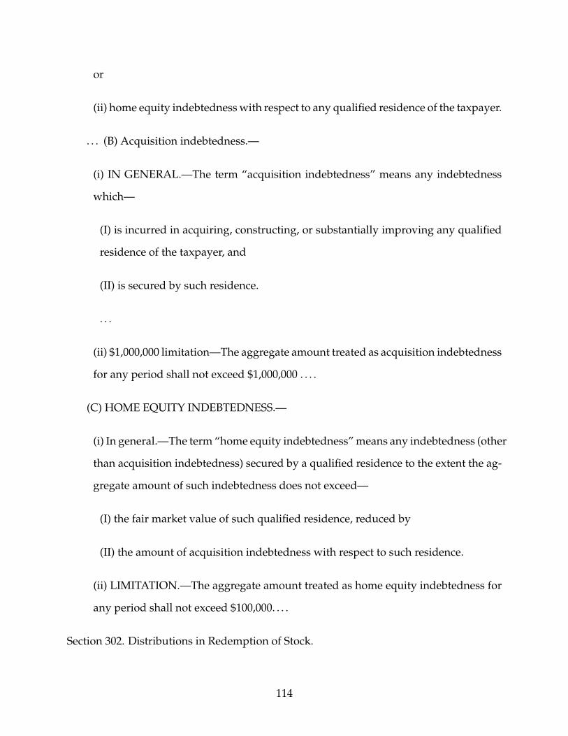
or

(ii) home equity indebtedness with respect to any qualified residence of the taxpayer.

. . . (B) Acquisition indebtedness.—

(i) IN GENERAL.—The term “acquisition indebtedness” means any indebtedness

which—

(I) is incurred in acquiring, constructing, or substantially improving any qualified

residence of the taxpayer, and

(II) is secured by such residence.

. . .

(ii) $1,000,000 limitation—The aggregate amount treated as acquisition indebtedness

for any period shall not exceed $1,000,000 . . . .

(C) HOME EQUITY INDEBTEDNESS.—

(i) In general.—The term “home equity indebtedness” means any indebtedness (other

than acquisition indebtedness) secured by a qualified residence to the extent the ag-

gregate amount of such indebtedness does not exceed—

(I) the fair market value of such qualified residence, reduced by

(II) the amount of acquisition indebtedness with respect to such residence.

(ii) LIMITATION.—The aggregate amount treated as home equity indebtedness for

any period shall not exceed $100,000. . . .

Section 302. Distributions in Redemption of Stock.

114

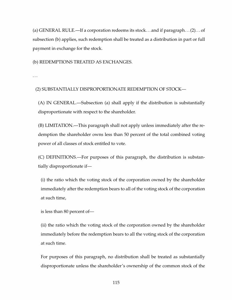
(a) GENERAL RULE.—If a corporation redeems its stock. . . and if paragraph. . . (2). . . of

subsection (b) applies, such redemption shall be treated as a distribution in part or full

payment in exchange for the stock.

(b) REDEMPTIONS TREATED AS EXCHANGES.

. . .

(2) SUBSTANTIALLY DISPROPORTIONATE REDEMPTION OF STOCK—

(A) IN GENERAL.—Subsection (a) shall apply if the distribution is substantially

disproportionate with respect to the shareholder.

(B) LIMITATION.—This paragraph shall not apply unless immediately after the re-

demption the shareholder owns less than 50 percent of the total combined voting

power of all classes of stock entitled to vote.

(C) DEFINITIONS.—For purposes of this paragraph, the distribution is substan-

tially disproportionate if—

(i) the ratio which the voting stock of the corporation owned by the shareholder

immediately after the redemption bears to all of the voting stock of the corporation

at such time,

is less than 80 percent of—

(ii) the ratio which the voting stock of the corporation owned by the shareholder

immediately before the redemption bears to all the voting stock of the corporation

at such time.

For purposes of this paragraph, no distribution shall be treated as substantially

disproportionate unless the shareholder’s ownership of the common stock of the

115

corporation (whether voting or nonvoting) after and before redemption also meets

the 80 percent requirement of the preceding sentence. . . .

(D) SERIES OF REDEMPTIONS.—This paragraph shall not apply to any redemption

made pursuant to a plan the purpose or effect of which is a series of redemptions re-

sulting in a distribution which (in the aggregate) is not substantially disproportionate

with respect to the shareholder.

116

Appendix B

Justifying stable scenarios

This appendix justifies the stable scenarios throughout the dissertation. In this appendix,

a circled rule fits the category under which it is listed. For example, if all three rules

are circled in the Triggered column, all three rules are triggered in that scenario. If δ1

and δ3 are circled in the Not Defeated column, only δ2 is defeated with respect to that

scenario. As a result, rules that are Binding with respect to a particular scenario are circled

in all three columns (because a rule that is circled in all three columns is triggered, not

conflicted, and not defeated).

The reason for the characterization of the rule is immediately under the rule. For example,

if T1 is immediately under the circled δ1 in the Triggered column, the justification for char-

acterizing δ1 as triggered in that scenario is Rule T1, which is in the relevant subsection

immediately above the chart.

117

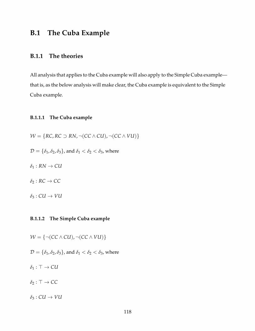
B.1 The Cuba Example

B.1.1 The theories

All analysis that applies to the Cuba example will also apply to the Simple Cuba example—

that is, as the below analysis will make clear, the Cuba example is equivalent to the Simple

Cuba example.

B.1.1.1 The Cuba example

W = {RC, RC ⊃ RN,¬(CC ∧ CU),¬(CC ∧VU)}

D = {δ1, δ2, δ3}, and δ1 < δ2 < δ3, where

δ1 : RN → CU

δ2 : RC → CC

δ3 : CU → VU

B.1.1.2 The Simple Cuba example

W = {¬(CC ∧ CU),¬(CC ∧VU)}

D = {δ1, δ2, δ3}, and δ1 < δ2 < δ3, where

δ1 : > → CU

δ2 : > → CC

δ3 : CU → VU

118

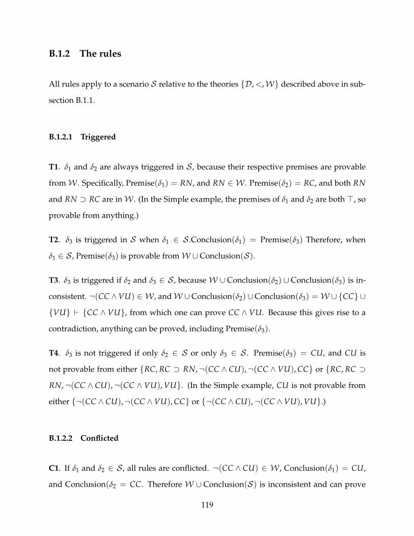
B.1.2 The rules

All rules apply to a scenario S relative to the theories {D,<,W} described above in sub-

section B.1.1.

B.1.2.1 Triggered

T1. δ1 and δ2 are always triggered in S , because their respective premises are provable

fromW . Specifically, Premise(δ1) = RN, and RN ∈ W . Premise(δ2) = RC, and both RN

and RN ⊃ RC are inW . (In the Simple example, the premises of δ1 and δ2 are both >, so

provable from anything.)

T2. δ3 is triggered in S when δ1 ∈ S .Conclusion(δ1) = Premise(δ3) Therefore, when

δ1 ∈ S , Premise(δ3) is provable fromW ∪Conclusion(S).

T3. δ3 is triggered if δ2 and δ3 ∈ S , becauseW ∪ Conclusion(δ2) ∪ Conclusion(δ3) is in-

consistent. ¬(CC∧VU) ∈ W , andW ∪Conclusion(δ2)∪Conclusion(δ3) =W ∪{CC} ∪

{VU} ` {CC ∧ VU}, from which one can prove CC ∧ VU. Because this gives rise to a

contradiction, anything can be proved, including Premise(δ3).

T4. δ3 is not triggered if only δ2 ∈ S or only δ3 ∈ S . Premise(δ3) = CU, and CU is

not provable from either {RC, RC ⊃ RN,¬(CC ∧ CU),¬(CC ∧ VU), CC} or {RC, RC ⊃

RN,¬(CC ∧ CU),¬(CC ∧ VU), VU}. (In the Simple example, CU is not provable from

either {¬(CC ∧ CU),¬(CC ∧VU), CC} or {¬(CC ∧ CU),¬(CC ∧VU), VU}.)

B.1.2.2 Conflicted

C1. If δ1 and δ2 ∈ S , all rules are conflicted. ¬(CC ∧ CU) ∈ W , Conclusion(δ1) = CU,

and Conclusion(δ2 = CC. Therefore W ∪ Conclusion(S) is inconsistent and can prove

119

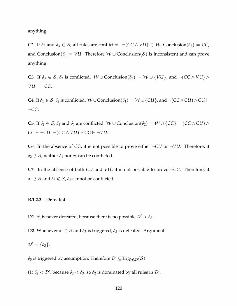
anything.

C2. If δ2 and δ3 ∈ S , all rules are conflicted. ¬(CC ∧ VU) ∈ W , Conclusion(δ2) = CC,

and Conclusion(δ3 = VU. Therefore W ∪ Conclusion(S) is inconsistent and can prove

anything.

C3. If δ3 ∈ S , δ2 is conflicted. W ∪ Conclusion(δ3) = W ∪ {VU}, and ¬(CC ∧ VU) ∧

VU ` ¬CC.

C4. If δ1 ∈ S , δ2 is conflicted.W∪Conclusion(δ1) =W∪{CU}, and ¬(CC∧CU)∧CU `

¬CC.

C5. If δ2 ∈ S , δ1 and δ3 are conflicted. W ∪Conclusion(δ2) = W ∪ {CC}. ¬(CC ∧ CU) ∧

CC ` ¬CU. ¬(CC ∧VU) ∧ CC ` ¬VU.

C6. In the absence of CC, it is not possible to prove either ¬CU or ¬VU. Therefore, if

δ2 6∈ S , neither δ1 nor δ3 can be conflicted.

C7. In the absence of both CU and VU, it is not possible to prove ¬CC. Therefore, if

δ1 6∈ S and δ3 6∈ S , δ2 cannot be conflicted.

B.1.2.3 Defeated

D1. δ3 is never defeated, because there is no possible D′ > δ3.

D2. Whenever δ1 ∈ S and δ3 is triggered, δ2 is defeated. Argument:

D′ = {δ3}.

δ3 is triggered by assumption. Therefore D′ ⊆TrigW ,D(S).

(1) δ2 < D′, because δ2 < δ3, so δ2 is dominated by all rules in D′.

120

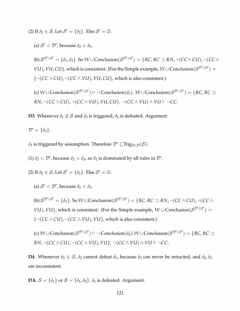
(2) If δ2 ∈ S , Let S ′ = {δ2}. Else S ′ = ∅.

(a) S ′ < D′, because δ2 < δ3.

(b) SD′/S ′ = {δ1, δ3}. SoW∪Conclusion(SD′/S ′) = {RC, RC ⊃ RN,¬(CC∧CU),¬(CC∧

VU), VU, CU}, which is consistent. (For the Simple example,W∪Conclusion(SD′/S ′) =

{¬(CC ∧ CU),¬(CC ∧VU), VU, CU}, which is also consistent.)

(c)W∪Conclusion(SD′/S ′) ` ¬Conclusion(δ2).W∪Conclusion(SD′/S ′) = {RC, RC ⊃

RN,¬(CC ∧ CU),¬(CC ∧VU), VU, CU}. ¬(CC ∧VU) ∧VU ` ¬CC.

D3. Whenever δ1 6∈ S and δ3 is triggered, δ2 is defeated. Argument:

D′ = {δ3}.

δ3 is triggered by assumption. Therefore D′ ⊆TrigW ,D(S).

(1) δ2 < D′, because δ2 < δ3, so δ2 is dominated by all rules in D′.

(2) If δ2 ∈ S , Let S ′ = {δ2}. Else S ′ = ∅.

(a) S ′ < D′, because δ2 < δ3.

(b) SD′/S ′ = {δ3}. SoW∪Conclusion(SD′/S ′) = {RC, RC ⊃ RN,¬(CC∧CU),¬(CC∧

VU), VU}, which is consistent. (For the Simple example, W ∪ Conclusion(SD′/S ′) =

{¬(CC ∧ CU),¬(CC ∧VU), VU}, which is also consistent.)

(c)W∪Conclusion(SD′/S ′) ` ¬Conclusion(δ2).W∪Conclusion(SD′/S ′) = {RC, RC ⊃

RN,¬(CC ∧ CU),¬(CC ∧VU), VU}. ¬(CC ∧VU) ∧VU ` ¬CC.

D4. Whenever δ3 ∈ S , δ2 cannot defeat δ1, because δ3 can never be retracted, and δ2, δ3

are inconsistent.

DA. S = {δ1} or S = {δ1, δ2}. δ1 is defeated. Argument:

121

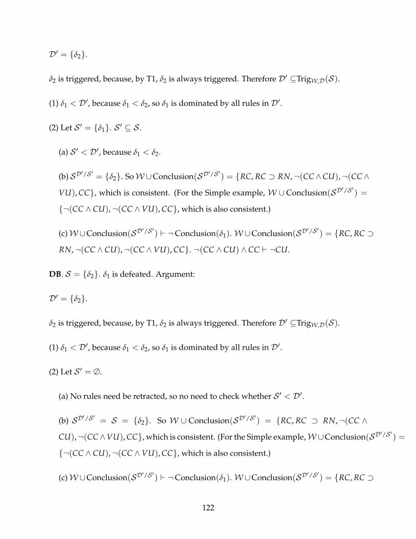
D′ = {δ2}.

δ2 is triggered, because, by T1, δ2 is always triggered. Therefore D′ ⊆TrigW ,D(S).

(1) δ1 < D′, because δ1 < δ2, so δ1 is dominated by all rules in D′.

(2) Let S ′ = {δ1}. S ′ ⊆ S .

(a) S ′ < D′, because δ1 < δ2.

(b) SD′/S ′ = {δ2}. SoW∪Conclusion(SD′/S ′) = {RC, RC ⊃ RN,¬(CC∧CU),¬(CC∧

VU), CC}, which is consistent. (For the Simple example, W ∪ Conclusion(SD′/S ′) =

{¬(CC ∧ CU),¬(CC ∧VU), CC}, which is also consistent.)

(c)W∪Conclusion(SD′/S ′) ` ¬Conclusion(δ1).W∪Conclusion(SD′/S ′) = {RC, RC ⊃

RN,¬(CC ∧ CU),¬(CC ∧VU), CC}. ¬(CC ∧ CU) ∧ CC ` ¬CU.

DB. S = {δ2}. δ1 is defeated. Argument:

D′ = {δ2}.

δ2 is triggered, because, by T1, δ2 is always triggered. Therefore D′ ⊆TrigW ,D(S).

(1) δ1 < D′, because δ1 < δ2, so δ1 is dominated by all rules in D′.

(2) Let S ′ = ∅.

(a) No rules need be retracted, so no need to check whether S ′ < D′.

(b) SD′/S ′ = S = {δ2}. So W ∪ Conclusion(SD′/S ′) = {RC, RC ⊃ RN,¬(CC ∧

CU),¬(CC∧VU), CC}, which is consistent. (For the Simple example,W∪Conclusion(SD′/S ′) =

{¬(CC ∧ CU),¬(CC ∧VU), CC}, which is also consistent.)

(c)W∪Conclusion(SD′/S ′) ` ¬Conclusion(δ1).W∪Conclusion(SD′/S ′) = {RC, RC ⊃

122

RN,¬(CC ∧ CU),¬(CC ∧VU), CC}. ¬(CC ∧ CU) ∧ CC ` ¬CU.

DC. S = ∅. δ1 is defeated. Argument:

D′ = {δ2}.

δ2 is triggered, because, by T1, δ2 is always triggered. Therefore D′ ⊆TrigW ,D(S).

(1) δ1 < D′, because δ1 < δ2, so δ1 is dominated by all rules in D′.

(2) Let S ′ = {∅}.

(a) No rules need be retracted, so no need to check whether S ′ < D′.

(b) SD′/S ′ = {δ2}. SoW∪Conclusion(SD′/S ′) = {RC, RC ⊃ RN,¬(CC∧CU),¬(CC∧

VU), CC}, which is consistent. (For the Simple example, W ∪ Conclusion(SD′/S ′) =

{¬(CC ∧ CU),¬(CC ∧VU), CC}, which is also consistent.)

(c)W∪Conclusion(SD′/S ′) ` ¬Conclusion(δ1)}.W∪Conclusion(SD′/S ′) = {RC, RC ⊃

RN,¬(CC ∧ CU),¬(CC ∧VU), CC}. ¬(CC ∧ CU) ∧ CC ` ¬CU.

123

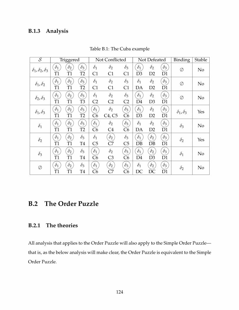
B.1.3 Analysis

Table B.1: The Cuba example

S Triggered Not Conflicted Not Defeated Binding Stable

δ1, δ2, δ3δ1 δ2 δ3 δ1 δ2 δ3 δ1 δ2 δ3 ∅ NoT1 T1 T2 C1 C1 C1 D3 D2 D1

δ1, δ2δ1 δ2 δ3 δ1 δ2 δ3 δ1 δ2 δ3 ∅ NoT1 T1 T2 C1 C1 C1 DA D2 D1

δ2, δ3δ1 δ2 δ3 δ1 δ2 δ3 δ1 δ2 δ3 ∅ NoT1 T1 T3 C2 C2 C2 D4 D3 D1

δ1, δ3δ1 δ2 δ3 δ1 δ2 δ3 δ1 δ2 δ3 δ1, δ3 YesT1 T1 T2 C6 C4, C5 C6 D3 D2 D1

δ1δ1 δ2 δ3 δ1 δ2 δ3 δ1 δ2 δ3 δ3 NoT1 T1 T2 C6 C4 C6 DA D2 D1

δ2δ1 δ2 δ3 δ1 δ2 δ3 δ1 δ2 δ3 δ2 YesT1 T1 T4 C5 C7 C5 DB DB D1

δ3δ1 δ2 δ3 δ1 δ2 δ3 δ1 δ2 δ3 δ1 NoT1 T1 T4 C6 C3 C6 D4 D3 D1

∅ δ1 δ2 δ3 δ1 δ2 δ3 δ1 δ2 δ3 δ2 NoT1 T1 T4 C6 C7 C6 DC DC D1

B.2 The Order Puzzle

B.2.1 The theories

All analysis that applies to the Order Puzzle will also apply to the Simple Order Puzzle—

that is, as the below analysis will make clear, the Order Puzzle is equivalent to the Simple

Order Puzzle.

124

B.2.1.1 The Order Puzzle

W = {W}

D = {δ1, δ2, δ3}, and δ1 < δ2 < δ3, where

δ1 : W → H

δ2 : W → ¬O

δ3 : H → O

B.2.1.2 The Simple Order Puzzle

W = ∅

D = {δ1, δ2, δ3}, and δ1 < δ2 < δ3, where

δ1 : > → H

δ2 : > → ¬O

δ3 : H → O

B.2.2 The rules

All rules apply to a scenario S relative to the theories {D,<,W} described above in sub-

section B.2.1.

125

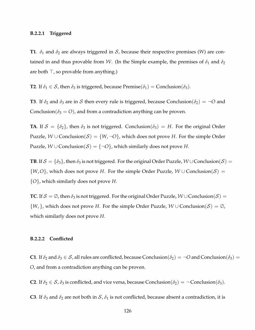
B.2.2.1 Triggered

T1. δ1 and δ2 are always triggered in S , because their respective premises (W) are con-

tained in and thus provable from W . (In the Simple example, the premises of δ1 and δ2

are both >, so provable from anything.)

T2. If δ1 ∈ S , then δ3 is triggered, because Premise(δ1) = Conclusion(δ3).

T3. If δ2 and δ3 are in S then every rule is triggered, because Conclusion(δ2) = ¬O and

Conclusion(δ3 = O), and from a contradiction anything can be proven.

TA. If S = {δ2}, then δ3 is not triggered. Conclusion(δ3) = H. For the original Order

Puzzle,W ∪ Conclusion(S) = {W,¬O}, which does not prove H. For the simple Order

Puzzle,W ∪Conclusion(S) = {¬O}, which similarly does not prove H.

TB. If S = {δ3}, then δ3 is not triggered. For the original Order Puzzle,W∪Conclusion(S) =

{W, O}, which does not prove H. For the simple Order Puzzle, W ∪ Conclusion(S) =

{O}, which similarly does not prove H.

TC. If S = ∅, then δ3 is not triggered. For the original Order Puzzle,W∪Conclusion(S) =

{W, }, which does not prove H. For the simple Order Puzzle,W ∪ Conclusion(S) = ∅,

which similarly does not prove H.

B.2.2.2 Conflicted

C1. If δ2 and δ3 ∈ S , all rules are conflicted, because Conclusion(δ2) = ¬O and Conclusion(δ3) =

O, and from a contradiction anything can be proven.

C2. If δ2 ∈ S , δ3 is conflicted, and vice versa, because Conclusion(δ2) = ¬Conclusion(δ3).

C3. If δ3 and δ2 are not both in S , δ1 is not conflicted, because absent a contradiction, it is

126

not possible to prove ¬H from the conclusions of the three rules.

C4. If δ2 /∈ S , δ3 is not conflicted. The largest possible S absent δ2 is S = {δ1, δ3}.

For the Order Puzzle,W∪Conclusion(S) = {W, H, O}, which does not prove¬Conclusion(δ3) =

¬O.

For the Simple Order Puzzle, W ∪ Conclusion(S) = {H, O}, which does not prove

¬Conclusion(δ3) = ¬O.

By monotonicity, if S were any subset of {δ1, δ3}, ¬Conclusion(δ3) could similarly not be

proven.

B.2.2.3 Defeated

D1. If δ3 is triggered and δ2 /∈ S , then δ2 is defeated. Argument:

S ′ = ∅.

D′ = {δ3}.

δ3 is triggered by assumption. Therefore D′ ⊆TrigW ,D(S).

(1) δ2 < D′, because δ2 < δ3, so δ2 is dominated by all rules in D′.

(2)

(a) S ′ < D′, because δ2 < δ3.

(b) If δ1 ∈ S , SD′/S ′ = {δ1, δ3}. So W ∪ Conclusion(SD′/S ′) = {H, O}, which is

consistent. Removing H does not make the set inconsistent, so this holds if δ1 /∈ S .

(c)W ∪Conclusion(SD′/S ′) ` ¬Conclusion(δ2).

127

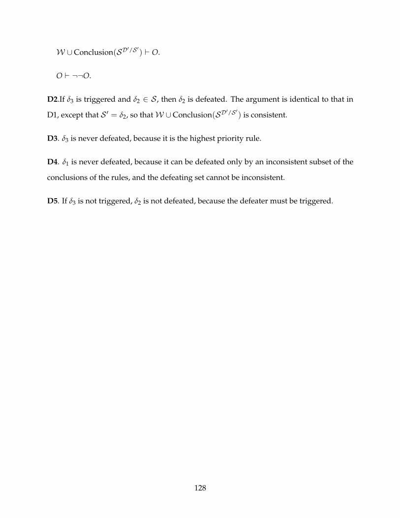
W ∪Conclusion(SD′/S ′) ` O.

O ` ¬¬O.

D2.If δ3 is triggered and δ2 ∈ S , then δ2 is defeated. The argument is identical to that in

D1, except that S ′ = δ2, so thatW ∪Conclusion(SD′/S ′) is consistent.

D3. δ3 is never defeated, because it is the highest priority rule.

D4. δ1 is never defeated, because it can be defeated only by an inconsistent subset of the

conclusions of the rules, and the defeating set cannot be inconsistent.

D5. If δ3 is not triggered, δ2 is not defeated, because the defeater must be triggered.

128

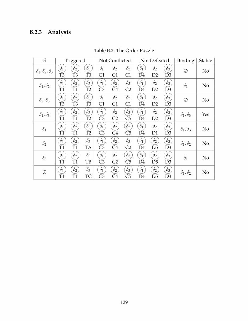
B.2.3 Analysis

Table B.2: The Order Puzzle

S Triggered Not Conflicted Not Defeated Binding Stable

δ1, δ2, δ3δ1 δ2 δ3 δ1 δ2 δ3 δ1 δ2 δ3 ∅ NoT3 T3 T3 C1 C1 C1 D4 D2 D3

δ1, δ2δ1 δ2 δ3 δ1 δ2 δ3 δ1 δ2 δ3 δ1 NoT1 T1 T2 C3 C4 C2 D4 D2 D3

δ2, δ3δ1 δ2 δ3 δ1 δ2 δ3 δ1 δ2 δ3 ∅ NoT3 T3 T3 C1 C1 C1 D4 D2 D3

δ1, δ3δ1 δ2 δ3 δ1 δ2 δ3 δ1 δ2 δ3 δ1, δ3 YesT1 T1 T2 C3 C2 C5 D4 D2 D3

δ1δ1 δ2 δ3 δ1 δ2 δ3 δ1 δ2 δ3 δ1, δ3 NoT1 T1 T2 C3 C4 C5 D4 D1 D3

δ2δ1 δ2 δ3 δ1 δ2 δ3 δ1 δ2 δ3 δ1, δ2 NoT1 T1 TA C3 C4 C2 D4 D5 D3

δ3δ1 δ2 δ3 δ1 δ2 δ3 δ1 δ2 δ3 δ1 NoT1 T1 TB C3 C2 C5 D4 D5 D3

∅ δ1 δ2 δ3 δ1 δ2 δ3 δ1 δ2 δ3 δ1, δ2 NoT1 T1 TC C3 C4 C5 D4 D5 D3

129

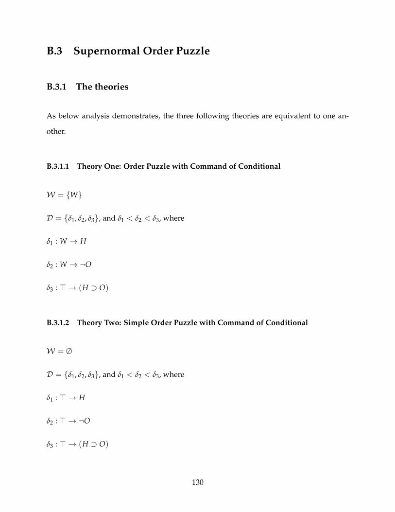
B.3 Supernormal Order Puzzle

B.3.1 The theories

As below analysis demonstrates, the three following theories are equivalent to one an-

other.

B.3.1.1 Theory One: Order Puzzle with Command of Conditional

W = {W}

D = {δ1, δ2, δ3}, and δ1 < δ2 < δ3, where

δ1 : W → H

δ2 : W → ¬O

δ3 : > → (H ⊃ O)

B.3.1.2 Theory Two: Simple Order Puzzle with Command of Conditional

W = ∅

D = {δ1, δ2, δ3}, and δ1 < δ2 < δ3, where

δ1 : > → H

δ2 : > → ¬O

δ3 : > → (H ⊃ O)

130

B.3.1.3 Theory Three: Supernormal Order Puzzle

W = {W}

D = {δ1, δ2, δ3}, and δ1 < δ2 < δ3, where

δ1 : > → (W ⊃ H)

δ2 : > → (W ⊃ ¬O)

δ3 : > → (H ⊃ O)

B.3.2 The rules

All rules apply to a scenario S relative to the theories {D,<,W} described above in sub-

section B.3.1.

B.3.2.1 Triggered

T1. All rules are always triggered. Either the premise of the rule is >, or the premise of

the rule is W and W ∈ W .

B.3.2.2 Conflicted

CA. If S = {δ1, δ2, δ3}, everything is conflicted, because W ⋃Conclusion(S) proves a

contradiction, O ∧ ¬O.

CB. If S = {δ1, δ2}, δ3 is not conflicted (notice this is different from the “normal” Order

Puzzle), because

131

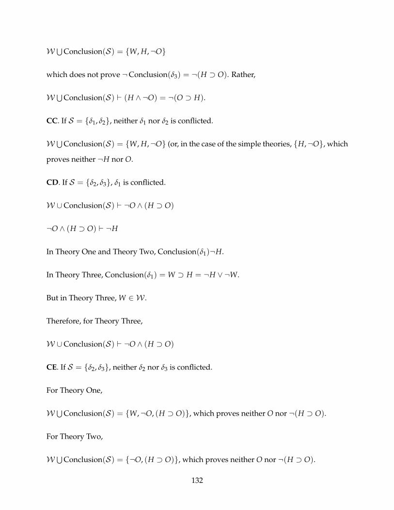
W ⋃Conclusion(S) = {W, H,¬O}

which does not prove ¬Conclusion(δ3) = ¬(H ⊃ O). Rather,

W ⋃Conclusion(S) ` (H ∧ ¬O) = ¬(O ⊃ H).

CC. If S = {δ1, δ2}, neither δ1 nor δ2 is conflicted.

W ⋃Conclusion(S) = {W, H,¬O} (or, in the case of the simple theories, {H,¬O}, which

proves neither ¬H nor O.

CD. If S = {δ2, δ3}, δ1 is conflicted.

W ∪Conclusion(S) ` ¬O ∧ (H ⊃ O)

¬O ∧ (H ⊃ O) ` ¬H

In Theory One and Theory Two, Conclusion(δ1)¬H.

In Theory Three, Conclusion(δ1) = W ⊃ H = ¬H ∨ ¬W.

But in Theory Three, W ∈ W .

Therefore, for Theory Three,

W ∪Conclusion(S) ` ¬O ∧ (H ⊃ O)

CE. If S = {δ2, δ3}, neither δ2 nor δ3 is conflicted.

For Theory One,

W ⋃Conclusion(S) = {W,¬O, (H ⊃ O)}, which proves neither O nor ¬(H ⊃ O).

For Theory Two,

W ⋃Conclusion(S) = {¬O, (H ⊃ O)}, which proves neither O nor ¬(H ⊃ O).

132

For Theory Three,

W ⋃Conclusion(S) = {W, (W ⊃ ¬O), (H ⊃ O)}, which proves neither ¬(W ⊃ ¬O)

(which would require proving O) nor ¬(H ⊃ O).

CF. If S = {δ1, δ3}, δ2 is conflicted.

In Theories One and Two, ¬Conclusion(δ2) = O.

Therefore, δ2 is conflicted ifW ⋃Conclusion(S) ` O.

Additionally, in Theories One and Two,

{H, (H ⊃ O)} ⊆ W ⋃Conclusion(S).

Therefore, in both Theory One and Theory Two,

W ⋃Conclusion(S) ` O, and thus δ2 is conflicted.

In Theory Three, ¬Conclusion(δ2) = ¬(W ⊃ ¬O) = ¬(¬O ∨ ¬W) = O ∧W.

W ⋃Conclusion(S) = {W, (W ⊃ H), (H ⊃ O)}.

Therefore, plainly,W ⋃Conclusion(S) ` O ∧W.

Thus, δ3 is conflicted in Theory Three.

CG. If S = {δ1, δ3}, neither δ1 nor δ3 is conflicted.

In all three theories, Conclusion(δ3) = H ⊃ O. For δ3 to be conflicted, the relevant

W ⋃Conclusion(S) would have to prove ¬(H ⊃ O) = ¬(O ∨ ¬H) = ¬O ∧ H.

In Theory One,

Conclusion(δ1) = H.

133

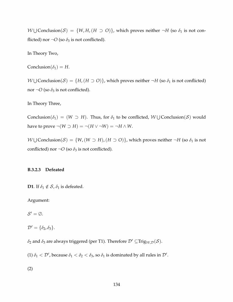
W ⋃Conclusion(S) = {W, H, (H ⊃ O)}, which proves neither ¬H (so δ1 is not con-

flicted) nor ¬O (so δ3 is not conflicted).

In Theory Two,

Conclusion(δ1) = H.

W ⋃Conclusion(S) = {H, (H ⊃ O)}, which proves neither ¬H (so δ1 is not conflicted)

nor ¬O (so δ3 is not conflicted).

In Theory Three,

Conclusion(δ1) = (W ⊃ H). Thus, for δ1 to be conflicted, W ⋃Conclusion(S) would

have to prove ¬(W ⊃ H) = ¬(H ∨ ¬W) = ¬H ∧W.

W ⋃Conclusion(S) = {W, (W ⊃ H), (H ⊃ O)}, which proves neither ¬H (so δ1 is not

conflicted) nor ¬O (so δ3 is not conflicted).

B.3.2.3 Defeated

D1. If δ1 /∈ S , δ1 is defeated.

Argument:

S ′ = ∅.

D′ = {δ2, δ3}.

δ2 and δ3 are always triggered (per T1). Therefore D′ ⊆TrigW ,D(S).

(1) δ1 < D′, because δ1 < δ2 < δ3, so δ1 is dominated by all rules in D′.

(2)

134

For Theory One:

(a) S ′ < D′ (because S ′ = ∅).

(b) SD′/S ′ = {δ2, δ3}.

SoW ∪Conclusion(SD′/S ′) = {W,¬O, (H ⊃ O)}, which is consistent.

(c)W ∪Conclusion(SD′/S ′) ` ¬H = ¬Conclusion(δ1).

For Theory Two:

(a) S ′ < D′ (because S ′ = ∅).

(b) SD′/S ′ = {δ2, δ3}.

SoW ∪Conclusion(SD′/S ′) = {¬O, (H ⊃ O)}, which is consistent.

(c)W ∪Conclusion(SD′/S ′) ` ¬H = ¬Conclusion(δ1).

For Theory Three:

(a) S ′ < D′ (because S ′ = ∅).

(b) SD′/S ′ = {δ2, δ3}.

SoW ∪Conclusion(SD′/S ′) = {W, (W ⊃ ¬O), (H ⊃ O)}, which is consistent.

(c)W ∪Conclusion(SD′/S ′) ` ¬H ∧W = ¬Conclusion(δ1).

D2. If δ1 ∈ S , then δ1 is defeated. The argument is identical to that in D1, except that

S ′ = δ1, so thatW ∪Conclusion(SD′/S ′) is consistent.

D3. δ3 is never defeated, because it is the highest priority rule.

D4. δ2 is never defeated. The only rule that dominates δ2 is δ3, but δ3 never works as the

135

defeating set for δ2 (notice the contrast here to the standard order puzzle).

For Theory One, {W, (H ⊃ O)} does not prove O.

For Theory Two, {(H ⊃ O)} does not prove O.

For Theory Three, {W, (H ⊃ O)} does not prove ¬(W ⊃ ¬O) = ¬(¬O ∨ ¬W) = O ∨W.

136

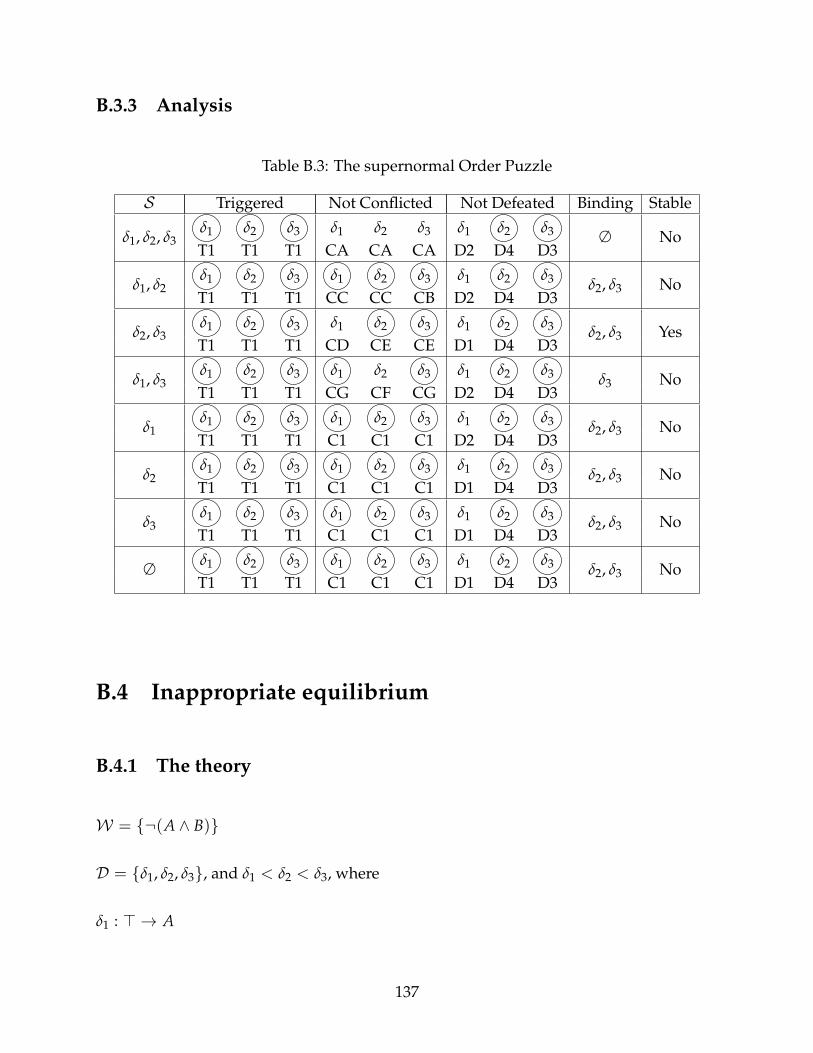
B.3.3 Analysis

Table B.3: The supernormal Order Puzzle

S Triggered Not Conflicted Not Defeated Binding Stable

δ1, δ2, δ3δ1 δ2 δ3 δ1 δ2 δ3 δ1 δ2 δ3 ∅ NoT1 T1 T1 CA CA CA D2 D4 D3

δ1, δ2δ1 δ2 δ3 δ1 δ2 δ3 δ1 δ2 δ3 δ2, δ3 NoT1 T1 T1 CC CC CB D2 D4 D3

δ2, δ3δ1 δ2 δ3 δ1 δ2 δ3 δ1 δ2 δ3 δ2, δ3 YesT1 T1 T1 CD CE CE D1 D4 D3

δ1, δ3δ1 δ2 δ3 δ1 δ2 δ3 δ1 δ2 δ3 δ3 NoT1 T1 T1 CG CF CG D2 D4 D3

δ1δ1 δ2 δ3 δ1 δ2 δ3 δ1 δ2 δ3 δ2, δ3 NoT1 T1 T1 C1 C1 C1 D2 D4 D3

δ2δ1 δ2 δ3 δ1 δ2 δ3 δ1 δ2 δ3 δ2, δ3 NoT1 T1 T1 C1 C1 C1 D1 D4 D3

δ3δ1 δ2 δ3 δ1 δ2 δ3 δ1 δ2 δ3 δ2, δ3 NoT1 T1 T1 C1 C1 C1 D1 D4 D3

∅ δ1 δ2 δ3 δ1 δ2 δ3 δ1 δ2 δ3 δ2, δ3 NoT1 T1 T1 C1 C1 C1 D1 D4 D3

B.4 Inappropriate equilibrium

B.4.1 The theory

W = {¬(A ∧ B)}

D = {δ1, δ2, δ3}, and δ1 < δ2 < δ3, where

δ1 : > → A

137

δ2 : > → B

δ3 : A→ ¬B

B.4.2 The rules

All rules apply to a scenario S relative to the theory {D,<,W} described above in sub-

section B.4.1.

B.4.2.1 Triggered

T1. δ1 and δ2 are always triggered, because each has the premise >.

T2. If δ1 ∈ S , δ3 is triggered. Conclusion(δ1) = Premise(δ3).

T3. If δ2, δ3 ∈ S , δ3 is triggered. Conclusion(δ2) ∧Conclusion(δ3) = B ∧ ¬B. Because this

is a contradiction, everything, including Premise(δ3) = A, can be proven.

TA. If {δ2} = S , then δ3 is not triggered. Premise(δ3) = A. W ⋃Conclusion(S) =

{¬(A ∧ B), B}, which is consistent and rather than proving Premise(δ3), actually proves

¬A.

TB. If {δ3} = S , then δ3 is not triggered. Premise(δ3) = A. W ⋃Conclusion(S) =

{¬(A ∧ B),¬B}, which does not prove Premise(δ3).

TC. If If ∅ = S , then δ3 is not triggered. Premise(δ3) = A. W ⋃Conclusion(S) =

{¬(A ∧ B)}, which does not prove Premise(δ3).

138

B.4.2.2 Conflicted

C1. If δ1, δ2 ∈ S everything is conflicted, becauseW ⋃Conclusion(S) proves a contradic-

tion, (A ∧ B) ∧ ¬(A ∧ B).

C2. If δ2, δ3 ∈ S everything is conflicted, becauseW ⋃Conclusion(S) proves a contradic-

tion, B ∧ ¬B.

C3. If δ1 ∈ S , then δ2 is conflicted. If δ1 ∈ S , then A,¬(A ∧ B) ∈ W ⋃Conclusion(S).

ThusW ⋃Conclusion(S) ` ¬B. By monotonicity, this will hold whether or not δ2, δ3 ∈ S .

C4. If S ⊆ {δ1, δ3}, then neither δ1 nor δ3 is conflicted. If {δ1, δ3} = {S}, thenW ⋃Conclusion(S) =

{A,¬B,¬(A ∧ B)}. Neither B nor ¬A can be proven from this, nor from any subset of it.

CA. If S = {δ2}, both δ1 and δ3 are conflicted.

W ⋃Conclusion(S) = {B,¬(A ∧ B)}

ThereforeW ⋃Conclusion(S) ` ¬A and δ1 is conflicted.

AdditionallyW ⋃Conclusion(S) ` B so δ3 is conflicted.

W ⋃Conclusion(S) is, however, consistent, so δ2 is not conflicted, as ¬B is not proven.

CB. If S = {δ3}, then δ2 is conflicted, as Conclusion(δ3) = ¬Conclusion(δ2).

CC. If S = ∅ then no rules are conflicted, as

W ⋃Conclusion(S) =W , and ¬(A ∧ B) does not prove ¬A,¬B, or B.

B.4.2.3 Defeated

D1. δ3 is never defeated, because it is the highest priority rule.

139

D2. If δ3 is triggered and δ2 /∈ S , δ2 is defeated.

S ′ = ∅.

D′ = {δ3}. δ3 is triggered by assumption.

(1) δ2 < δ′3.

(2)

(a) S ′ < D′ (because S ′ = ∅).

(b) If δ1 ∈ S ,

W ∪Conclusion(SD′/S ′) = {¬B, A,¬(A ∧ B)}, which is consistent.

If δ1 /∈ S ,

W ∪Conclusion(SD′/S ′) = {¬B,¬(A ∧ B)}, which is consistent.

(c) If δ1 /∈ S ,

W∪Conclusion(SD′/S ′) = {¬B,¬(A∧B)}, which proves¬B, which is¬Conclusion(δ2).

By monotonicity, this holds if δ1 ∈ S .

D3. If δ3 is triggered and δ2 ∈ S , then δ2 is defeated. The argument is identical to that in

D2, except that S ′ = δ2, so thatW ∪Conclusion(SD′/S ′) is consistent.

D4. If δ3 is not triggered and not in S , δ2 is not defeated, as there is no rule that dominates

it available to defeat it.

DA. If S = {δ2}, δ1 is defeated.

S ′ = ∅.

140

D′ = {δ2}. δ2 is always triggered, by T1, and δ2 is not defeated, by D4.

(1) δ1 < δ′2.

(2)

(a) S ′ < D′ (because S ′ = ∅).

(b)W ∪Conclusion(SD′/S ′) = {B,¬(A ∧ B)}, which is consistent.

(c)W ∪Conclusion(SD′/S ′) proves ¬A, which is ¬Conclusion(δ1).

DB. If S = {δ3}, δ1 is not defeated. The only possible defeater is δ2, but Conclusion(δ2) is

not consistent with Conclusion(δ3), and δ3 cannot be retracted, because δ2 < δ3.

DC. If S = {∅}, δ1 is defeated.

S ′ = ∅.

D′ = {δ2}. δ2 is always triggered, by T1, and δ2 is not defeated, by D4.

(1) δ1 < δ′2.

(2)

(a) S ′ < D′ (because S ′ = ∅).

(b)W ∪Conclusion(SD′/S ′) = {B,¬(A ∧ B)}, which is consistent.

(c)W ∪Conclusion(SD′/S ′) proves ¬A, which is ¬Conclusion(δ1).

141

B.4.3 Analysis

Table B.4: Inappropriate equilibrium

S Triggered Not Conflicted Not Defeated Binding Stable

δ1, δ2, δ3δ1 δ2 δ3 δ1 δ2 δ3 δ1 δ2 δ3 ∅ NoT1 T1 T2 C1 C1 C1 D5 D3 D1

δ1, δ2δ1 δ2 δ3 δ1 δ2 δ3 δ1 δ2 δ3 ∅ NoT1 T1 T2 C1 C1 C1 D5 D3 D1

δ2, δ3δ1 δ2 δ3 δ1 δ2 δ3 δ1 δ2 δ3 ∅ NoT1 T1 T3 C2 C2 C2 D5 D3 D1

δ1, δ3δ1 δ2 δ3 δ1 δ2 δ3 δ1 δ2 δ3 δ1, δ3 YesT1 T1 T2 C4 C3 C4 D5 D2 D1

δ1δ1 δ2 δ3 δ1 δ2 δ3 δ1 δ2 δ3 δ1, δ3 NoT1 T1 T2 C4 C3 C4 D5 D2 D1

δ2δ1 δ2 δ3 δ1 δ2 δ3 δ1 δ2 δ3 δ2 YesT1 T1 TA CA CA CA DA D4 D1

δ3δ1 δ2 δ3 δ1 δ2 δ3 δ1 δ2 δ3 δ1 NoT1 T1 TB C4 CB C4 DB D4 D1

∅ δ1 δ2 δ3 δ1 δ2 δ3 δ1 δ2 δ3 δ2 NoT1 T1 TC CC CC CC DC D4 D1

142

B.5 Supernormal inappropriate equilibrium

B.5.1 The theory

W = {¬(A ∧ B)}

D = {δ1, δ2, δ3}, and δ1 < δ2 < δ3, where

δ1 : > → A

δ2 : > → B

δ′3 : > → (A ⊃ ¬B)

Note that Conclusion(δ′3) is equivalent to ¬(A∧ B). Thus δ3’ adds no information to what

is already contained inW .

B.5.2 The rules

All rules apply to a scenario S relative to the theory {D,<,W} described above in sub-

section B.5.1.

B.5.2.1 Triggered

T1. All rules are always triggered, because the premise of every rule is >.

143

B.5.2.2 Conflicted

C1. If δ1, δ2 ∈ S everything is conflicted, becauseW ⋃Conclusion(S) proves a contradic-

tion, (A ∧ B) ∧ ¬(A ∧ B).

C2. If δ2 ∈ S , then δ1 is conflicted. If δ2 ∈ {S}, then B,¬(A ∧ B) ∈ W ⋃Conclusion(S).

ThusW ⋃Conclusion(S) ` ¬A. By monotonicity, this will hold whether or not δ1, δ′3 ∈ S .

C3. If δ1 ∈ S , then δ2 is conflicted. If δ1 ∈ {S}, then A,¬(A ∧ B) ∈ W ⋃Conclusion(S),

ThusW ⋃Conclusion(S) ` ¬B. By monotonicity, this will hold whether or not δ2, δ′3 ∈ S .

C4. If S ⊆ {δ2, δ′3}, then neither δ2 nor δ′3 is conflicted. If {δ2, δ′3} = {S}, thenW ⋃Conclusion(S) =

{B,¬(A ∧ B)}. Neither ¬B nor A ∧ B can be proven from this, nor from any subset of it.

C4. If S ⊆ {δ1, δ′3}, then neither δ1 nor δ′3 is conflicted. If {δ1, δ′3} = S , thenW ⋃Conclusion(S) =

{A,¬(A ∧ B)}. Neither ¬A nor A ∧ B can be proven from this, nor from any subset of it.

C6. If S ⊆ {δ′3}, then nothing is conflicted. If {δ′3} = S , then W ⋃Conclusion(S) =

{¬(A ∧ B)}. None of ¬A, ¬B, or A ∧ B can be proven from this, nor from any subset of it

(i.e., ∅).

B.5.2.3 Defeated

D1. δ3 is never defeated, because it is the highest priority rule.

D2. If δ1 /∈ S , δ1 is defeated.

S ′ = ∅.

D′ = {δ2}. δ2 is always triggered, per T1.

(1) δ1 < δ2.

144

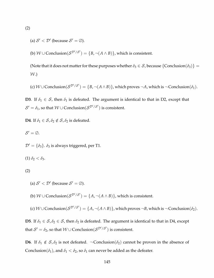
(2)

(a) S ′ < D′ (because S ′ = ∅).

(b)W ∪Conclusion(SD′/S ′) = {B,¬(A ∧ B)}, which is consistent.

(Note that it does not matter for these purposes whether δ3 ∈ S , because {Conclusion(δ3)} =

W .)

(c)W∪Conclusion(SD′/S ′) = {B,¬(A∧B)}, which proves¬A, which is¬Conclusion(δ1).

D3. If δ1 ∈ S , then δ1 is defeated. The argument is identical to that in D2, except that

S ′ = δ1, so thatW ∪Conclusion(SD′/S ′) is consistent.

D4. If δ1 ∈ S , δ2 /∈ S , δ2 is defeated.

S ′ = ∅.

D′ = {δ3}. δ3 is always triggered, per T1.

(1) δ2 < δ3.

(2)

(a) S ′ < D′ (because S ′ = ∅).

(b)W ∪Conclusion(SD′/S ′) = {A,¬(A ∧ B)}, which is consistent.

(c)W∪Conclusion(SD′/S ′) = {A,¬(A∧B)}, which proves¬B, which is¬Conclusion(δ2).

D5. If δ1 ∈ S , δ2 ∈ S , then δ2 is defeated. The argument is identical to that in D4, except

that S ′ = δ2, so thatW ∪Conclusion(SD′/S ′) is consistent.

D6. If δ1 /∈ S , δ2 is not defeated. ¬Conclusion(δ2) cannot be proven in the absence of

Conclusion(δ1), and δ1 < δ2, so δ1 can never be added as the defeater.

145

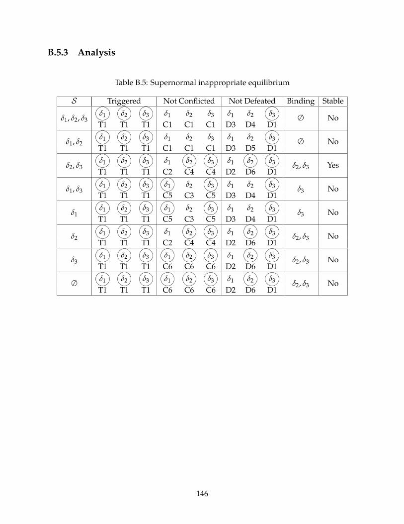
B.5.3 Analysis

Table B.5: Supernormal inappropriate equilibrium

S Triggered Not Conflicted Not Defeated Binding Stable

δ1, δ2, δ3δ1 δ2 δ3 δ1 δ2 δ3 δ1 δ2 δ3 ∅ NoT1 T1 T1 C1 C1 C1 D3 D4 D1

δ1, δ2δ1 δ2 δ3 δ1 δ2 δ3 δ1 δ2 δ3 ∅ NoT1 T1 T1 C1 C1 C1 D3 D5 D1

δ2, δ3δ1 δ2 δ3 δ1 δ2 δ3 δ1 δ2 δ3 δ2, δ3 YesT1 T1 T1 C2 C4 C4 D2 D6 D1

δ1, δ3δ1 δ2 δ3 δ1 δ2 δ3 δ1 δ2 δ3 δ3 NoT1 T1 T1 C5 C3 C5 D3 D4 D1

δ1δ1 δ2 δ3 δ1 δ2 δ3 δ1 δ2 δ3 δ3 NoT1 T1 T1 C5 C3 C5 D3 D4 D1

δ2δ1 δ2 δ3 δ1 δ2 δ3 δ1 δ2 δ3 δ2, δ3 NoT1 T1 T1 C2 C4 C4 D2 D6 D1

δ3δ1 δ2 δ3 δ1 δ2 δ3 δ1 δ2 δ3 δ2, δ3 NoT1 T1 T1 C6 C6 C6 D2 D6 D1

∅ δ1 δ2 δ3 δ1 δ2 δ3 δ1 δ2 δ3 δ2, δ3 NoT1 T1 T1 C6 C6 C6 D2 D6 D1

146