An Implementation of a Free-Variable Tableaux for KLM Preferential Logic P of Nonmonotonic Reasoning: The Theorem Prover FreeP 1.0

An Implementation of a Free-Variable Tableauxfor KLM Preferential Logic P of Nonmonotonic

Reasoning: The Theorem Prover FreeP 1.0

Laura Giordano1, Valentina Gliozzi2, Nicola Olivetti3, and Gian Luca Pozzato2

1 Dip. di Informatica - Univ. Piemonte O. “A. Avogadro”[email protected]

2 Dip. di Informatica - Universita di Torino{gliozzi,pozzato}@di.unito.it

3 LSIS-UMR CNRS 6168 Univ. “P. Cezanne”[email protected]

Abstract. We present FreeP 1.0, a theorem prover for the KLM pref-erential logic P of nonmonotonic reasoning. FreeP 1.0 is a SICStus Pro-log implementation of a free-variables, labelled tableau calculus for P,obtained by introducing suitable modalities to interpret conditional as-sertions. The performances of FreeP 1.0 are promising. FreeP 1.0 canbe downloaded at http:// www.di.unito.it/ ∼pozzato/FreeP 1.0.

1 Introduction

The work of Kraus, Lehmann and Magidor (KLM) in the early 90s [1] is a mile-stone in the area of nonmonotonic reasoning. The postulates outlined by KLMhave been widely accepted as the “conservative core” of nonmonotonic reason-ing: they correspond to properties that any concrete reasoning mechanism shouldsatisfy. Many different approaches to nonmonotonic reasoning are characterizedby the properties of two of the KLM logics, namely preferential logic P andrational logic R [2].

According to the KLM framework, a defeasible knowledge base is representedby a (finite) set of nonmonotonic conditionals of the form A |∼ B, whose readingis normally (or typically) the A’s are B’s. The operator “|∼” is nonmonotonic, inthat A |∼ B does not imply A ∧ C |∼ B. For instance, a knowledge base K maycontain sumo wrestler |∼ fat , sumo wrestler |∼ sumo lover , sumo lover |∼ ¬fat ,whose meaning is that sumo wrestlers are typically fat, sumo wrestlers typicallylove sumo, but people loving sumo typically are not fat. If |∼ were interpretedas classical implication, one would get sumo wrestler |∼ ⊥, i.e. typically thereare not sumo wrestlers, thereby obtaining a trivial knowledge base. One canderive new conditional assertions from the knowledge base by means of a set ofinference rules, without incurring the trivializing conclusions of classical logic.In KLM framework, the set of inference rules defines some fundamental typesof inference systems, namely, from the strongest to the weakest: Rational (R),Preferential (P), Loop-Cumulative (CL), and Cumulative (C) logic.

R. Basili and M.T. Pazienza (Eds.): AI*IA 2007, LNAI 4733, pp. 84–96, 2007.c© Springer-Verlag Berlin Heidelberg 2007

A Free-Variable Tableaux for KLM Preferential Logic P 85

In this paper we focus on Preferential logic P. Concerning the above exam-ple, in preferential logic P one can infer sumo lover ∧ sumo wrestler |∼ fat , givingpreference to more specific information, and that sumo lover |∼ ¬sumo wrestler .From a semantic point of view, the models of preferential logic P are possible-world structures equipped with a preference relation < among worlds. The mean-ing of a conditional assertion A |∼ B is that B holds in the most preferred worldswhere A holds.

In [3] an analytic tableau calculus for propositional P is introduced. The basicidea there is to interpret the preference relation < as an accessibility relation: aconditional A |∼ B holds in a model if B is true in all worlds satisfying A thatare minimal wrt <. The calculus provides a sort of run-time translation of P intoGodel-Lob modal logic of provability G. The relation with G is motivated by thefact that we assume, following KLM, the so-called smoothness condition, which isrelated to the well-known limit assumption. This condition ensures that minimalA-worlds exist whenever there are A-worlds, by preventing infinitely descendingchains of worlds. This condition is therefore ensured by the finite-chain condi-tion on the accessibility relation (as in modal logic G). The resulting calculus,called T PT, is a non-labelled, sound, complete and terminating proof methodfor the logic P. In [4] a SICStus Prolog implementation of T PT is presented.The program, called KLMLean 2.0, is inspired to the “lean” methodology, and,as far as we know, it is the first theorem prover for the preferential logic P.

We extend our work on efficient theorem proving for KLM logics by intro-ducing FreeP 1.0, a theorem prover for preferential logic P that implementsa free-variable tableau calculus for this logic. Free-variable tableaux are a well-known and well-established technique for first order theorem proving [5], whosebasic idea is to adopt free-variables as a meta-linguistic device for representingall labels/worlds that can be used in a proof search. To reduce the search space,the instantiation of these free-variables is postponed until more information isavailable (for instance to close a branch). Recently, Beckert and Gore have pre-sented the theoretical foundations to extend the free-variable tableaux techniqueto all 15 basic propositional modal logics [6].

In our paper, we first introduce a labelled tableau calculus for the preferentiallogic P, based on the same translation into G adopted by T PT. This calculus,called LABP, can be straightforwardly derived from the labelled calculus T RT

for the rational logic R introduced in [7]. We then show that LABP can beeasily turned into a terminating calculus. Last, we present FreeP 1.0, an im-plementation of a free-variables version of LABP in SICStus Prolog. This lastpoint is the main contribution of the paper.

2 KLM Preferential Logic P

In this section we briefly recall the axiomatization and semantics of the prefer-ential logic P. For a complete description of KLM systems, see [1] and [8]. Thelanguage L we consider is defined from a set of propositional variables ATM ,the boolean connectives and the conditional operator |∼. We use A, B, C, ... to

86 L. Giordano et al.

denote propositional formulas, whereas F, G, ... are used to denote all formulas(even conditionals). The formulas of L are defined as follows: if A is a propo-sitional formula, A ∈ L; if A and B are propositional formulas, A |∼ B ∈ L;if F is a boolean combination of formulas of L, F ∈ L. L corresponds to thefragment of the language of conditional logics without nested occurrences of theconditional operator |∼.

The axiomatization of P consists of all axioms and rules of propositionalcalculus together with the following axioms and rules (�PC denotes provabilityin the propositional calculus, whereas � denotes provability in P):

• REF. A |∼ A (reflexivity)• LLE. If �PC A ↔ B, then � (A |∼ C) → (B |∼ C) (left logical equivalence)• RW. If �PC A → B, then � (C |∼ A) → (C |∼ B) (right weakening)• AND. ((A |∼ B) ∧ (A |∼ C)) → (A |∼ B ∧ C)• CM. ((A |∼ B) ∧ (A |∼ C)) → (A ∧ B |∼ C) (cautious monotonicity)• OR. ((A |∼ C) ∧ (B |∼ C)) → (A ∨ B |∼ C)

The semantics of P is defined by considering possible world structures with apreference relation (a strict partial order) w < w′ whose meaning is that w ispreferred to w′. We have that A |∼ B holds in a model M if B holds in allminimal A-worlds (w.r.t. <). This definition makes sense provided minimal A-worlds exist (whenever there are A-worlds). This is ensured by the smoothnesscondition in the next definition.

Definition 1 (Semantics of P, Definition 16 in [1]). A preferential modelis a triple M = 〈W , <, V 〉 where: W is a non-empty set of items called worlds;< is an irreflexive and transitive relation on W; V is a function V : W �−→pow(ATM ), which assigns to every world w the set of atoms holding in thatworld. We define the truth conditions for a formula F as follows: (i) if F is aboolean combination of formulas, M, w |= F is defined as for propositional logic;(ii) let A be a propositional formula; we define Min<(A) = {w ∈ W | M, w |= Aand ∀w′, w′ < w implies M, w′ |= A}; (iii) M, w |= A |∼ B if for all w′ ∈ W, ifw′ ∈ Min<(A) then M, w′ |= B.

The relation < satisfies the following smoothness condition: if M, w |= Athen w ∈ Min<(A) or ∃w′ ∈ Min<(A) such that w′ < w.

We say that a formula F is valid in a model M (M |= F ), if M, w |= F forevery w ∈ W. A formula is valid if it is valid in every model M.

3 A Labelled Tableau Calculus for Preferential Logic P

In this section we present a labelled tableau calculus for preferential logic P.This calculus, called LABP from LABelled P, follows the same intuition asthe calculus T PT introduced in [3], i.e. to interpret the preference relation as anaccessibility relation, thus implementing a sort of run-time translation into modallogic G. LABP is straightforwardly derived from the labelled calculus T RT forrational logic R [7], by removing rule (<), corresponding to modularity thatdifferentiates P from R.


(AX) Γ , x : P, x : ¬P with P ∈ ATMΓ , x : ¬¬F

Γ , x : F

Γ , u : ¬(A |∼ B)

Γ , u : A |∼ B

Γ , u : A |∼ B, x : ¬A

Γ , x : A, x : �¬A, x : ¬B

Γ , u : A |∼ B, x : ¬�¬A Γ , u : A |∼ B, x : B

Γ , x : ¬�¬A

Γ , y < x, y : A, y : �¬A,ΓMx−→y

Γ , x : F ∧ G Γ , x : ¬(F ∧ G)

Γ , x : F, x : G Γ , x : ¬F Γ , x : ¬G

x new

y newlabel

x occurs in Γ

label(¬)

(|∼+)

(|∼−)

(�−) (∧−)(∧+)

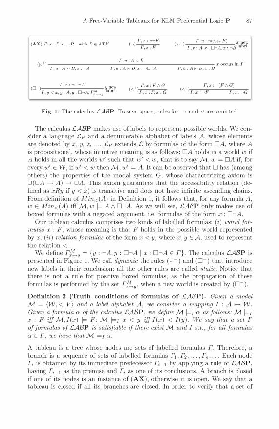
Fig. 1. The calculus LABP. To save space, rules for → and ∨ are omitted.

The calculus LABP makes use of labels to represent possible worlds. We con-sider a language LP and a denumerable alphabet of labels A, whose elementsare denoted by x, y, z, .... LP extends L by formulas of the form �A, where Ais propositional, whose intuitive meaning is as follows: �A holds in a world w ifA holds in all the worlds w′ such that w′ < w, that is to say M, w |= �A if, forevery w′ ∈ W , if w′ < w then M, w′ |= A. It can be observed that � has (amongothers) the properties of the modal system G, whose characterizing axiom is�(�A → A) → �A. This axiom guarantees that the accessibility relation (de-fined as xRy if y < x) is transitive and does not have infinite ascending chains.From definition of Min<(A) in Definition 1, it follows that, for any formula A,w ∈ Min<(A) iff M, w |= A ∧ �¬A. As we will see, LABP only makes use ofboxed formulas with a negated argument, i.e. formulas of the form x : �¬A.

Our tableau calculus comprises two kinds of labelled formulas: (i) world for-mulas x : F , whose meaning is that F holds in the possible world representedby x; (ii) relation formulas of the form x < y, where x, y ∈ A, used to representthe relation <.

We define Γ Mx→y = {y : ¬A, y : �¬A | x : �¬A ∈ Γ}. The calculus LABP is

presented in Figure 1. We call dynamic the rules (|∼−) and (�−) that introducenew labels in their conclusion; all the other rules are called static. Notice thatthere is not a rule for positive boxed formulas, as the propagation of theseformulas is performed by the set Γ M

x→y, when a new world is created by (�−).

Definition 2 (Truth conditions of formulas of LABP). Given a modelM = 〈W , <, V 〉 and a label alphabet A, we consider a mapping I : A �→ W.Given a formula α of the calculus LABP, we define M |=I α as follows: M |=I

x : F iff M, I(x) |= F ; M |=I x < y iff I(x) < I(y). We say that a set Γof formulas of LABP is satisfiable if there exist M and I s.t., for all formulasα ∈ Γ , we have that M |=I α.

A tableau is a tree whose nodes are sets of labelled formulas Γ . Therefore, abranch is a sequence of sets of labelled formulas Γ1, Γ2, . . . , Γn, . . . Each nodeΓi is obtained by its immediate predecessor Γi−1 by applying a rule of LABP,having Γi−1 as the premise and Γi as one of its conclusions. A branch is closedif one of its nodes is an instance of (AX), otherwise it is open. We say that atableau is closed if all its branches are closed. In order to verify that a set of


formulas Γ is unsatisfiable, we label all the formulas in Γ with a new label x,and verify that the resulting set of labelled formulas has a closed tableau.

The calculus LABP is sound and complete wrt the semantics. To save space,we omit the proofs, which are very similar to the ones for T RT in [7].

Theorem 1 (Soundness and Completeness of LABP). Given a set of for-mulas Γ , it is unsatisfiable if and only if there is a closed tableau in LABPstarting with Γ .

Let us now refine the calculus LABP in order to ensure termination. In gen-eral, non-termination in labelled tableau calculi can be caused by two differentreasons: 1. dynamic rules can generate infinitely-many worlds, thus creating in-finite branches; 2. some rules copy their principal formula in their conclusion(s),therefore they can be reapplied over the same formula without any control.

As far as LABP is concerned, we can show that the first source of non termi-nation (point 1) cannot occur. Indeed, similarly to T RT, we have that the onlyrules that can introduce new labels in the tableau are (|∼−) and (�−). It can beproven that there can be only finitely many applications of these rules in a proofsearch. Intuitively, the rule (|∼−) can be applied only once for each negated con-ditional occurring in the initial set Γ (hence it introduces only a finite numberof labels). Furthermore, the generation of infinite branches due to the interplaybetween rules (|∼+) and (�−) cannot occur. Indeed, each application of (�−)to a formula x : ¬�¬A (introduced by (|∼+)) adds the formula y : �¬A to theconclusion, so that (|∼+) can no longer consistently introduce y : ¬�¬A. This isdue to the properties of �, that are similar to the properties of the correspondingmodality of modal system G.

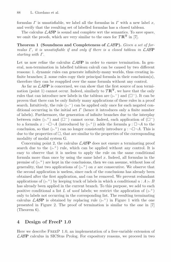
Concerning point 2, the calculus LABP does not ensure a terminating proofsearch due to the (|∼+) rule, which can be applied without any control. It iseasy to observe that it is useless to apply the rule on the same conditionalformula more than once by using the same label x. Indeed, all formulas in thepremise of (|∼+) are kept in the conclusions, then we can assume, without loss ofgenerality, that two applications of (|∼+) on x are consecutive. We observe thatthe second application is useless, since each of the conclusions has already beenobtained after the first application, and can be removed. We prevent redundantapplications of (|∼+) by keeping track of labels in which a conditional u : A |∼ Bhas already been applied in the current branch. To this purpose, we add to eachpositive conditional a list L of used labels; we restrict the application of (|∼+)only to labels not occurring in the corresponding list. The resulting terminatingcalculus LABP is obtained by replacing rule (|∼+) in Figure 1 with the onepresented in Figure 2. The proof of termination is similar to the one in [7](Theorem 6).

4 Design of FreeP 1.0

Here we describe FreeP 1.0, an implementation of a free-variable extension ofLABP calculus in SICStus Prolog. For expository reasons, we proceed in two


Γ , u : A |∼ B(|∼+)

with x �∈ L

L

L, x L, x L, xΓ , x : ¬A, u : A |∼ B Γ , x : ¬�¬A, u : A |∼ B Γ , x : B , u : A |∼ B

Fig. 2. The rule (|∼+) in the terminating tableau calculus LABP

steps. First, in section 4.1 we present a simple implementation of LABP thatdoes not use free-variables, yet. Second, in section 4.2 we refine it by introducingfree-variables in order to increase its performances. Intuitively, this refinementconsists in the fact that the (|∼+) rule introduces a free-variable in all its con-clusions, rather than immediately choosing the label to use. The free-variableswill then be instantiated to close a branch with an axiom, thus the choice of thelabel is postponed as much as possible.

4.1 A Simple Implementation of LABP (Without Free-Variables)

The Prolog program consists of a set of clauses, each representing a tableau ruleor axiom; the proof search is provided for free by the mere depth-first searchmechanism of Prolog, without any additional ad hoc mechanism. We representeach node of a proof tree (i.e. set of formulas) by a Prolog list. A world formulax : A is represented by a pair [x,a], whereas a relation formula x < y isrepresented by a triple [x,<,y]. The tableau calculus is implemented by thepredicate prove(Gamma,Cond,Labels,Tree), which succeeds if and only if theset of formulas Γ , represented by the list Gamma, is unsatisfiable. Cond is a listrepresenting the set of used conditionals, and it is needed in order to controlthe application of the rule (|∼+), as described in the previous section. More indetail, the elements of Cond are pairs of the form [A=>B,Used], where Used is aProlog list containing all the labels that have already been used to apply (|∼+)on x : A |∼ B in the current branch. As we will discuss later in this section,this allows to apply this rule in a controlled way, ensuring termination of theproof search. Labels is the list of labels introduced in the current branch. Whenprove succeeds, Tree contains a representation of a closed tableau. For instance,to prove that A |∼ B ∧C, ¬(A |∼ C) is unsatisfiable in P, one queries FreeP 1.0

with the goal prove([[x,a => (b and c)], [x,neg (a => c)]],[ ], [x],Tree). The string “=>” is used to represent the conditional operator |∼, “and” isused to denote ∧, and so on. Each clause of prove implements one axiom or ruleof the tableau calculus; for example, the clause implementing (|∼−) is as follows:

prove(Gamma,Cond,Labels,tree(. . .)):-select([X,neg (A => B)],Gamma,NewG),!,newLabel(Labels,Y),prove([[Y,neg B]|[[Y,box neg A]|[[Y,A]|NewG]]],Cond,[Y|Labels],. . .).

The clause for (|∼−) is applied when a formula x : ¬(A |∼ B) belongs to Γ . Thepredicate select removes x : ¬(A |∼ B) from Gamma, then the predicate prove isrecursively invoked on the only conclusion of the rule. The predicate newLabelis used to generate a new label Y not occurring in the current branch.


To search a derivation of a set of formulas Γ , FreeP 1.0 proceeds as follows:first of all, if Γ is an instance of (AX), the goal will succeed immediately byusing the clause for the axioms. If it is not, then the first applicable rule willbe chosen, e.g. if Gamma contains a formula [X,neg(neg F)], then the clausefor (¬) rule will be used, invoking prove on its unique conclusion. FreeP 1.0

proceeds in a similar way for the other rules. The ordering of the clauses is suchthat the boolean rules are applied before the other ones. Let us now analyze thecrucial rule (|∼+), which is implemented by the two following clauses:

prove(Gamma,Cond,Labels,tree(...)):-member([ ,A=>B],Gamma),\+member([A=>B, ],Cond),!,member(X,Labels),!,prove([[X,A->B]|Gamma],[[A=>B,[X]]|Cond],Labels,...),prove([[X,neg box neg A]|Gamma],[[A=>B,[X]]|Cond],...).

prove(Gamma,Cond,Labels,tree(...)):-member([ ,A=>B],Gamma),select([A=>B,Used],Cond,NewCond),member(X,Labels),\+member(X,Used),!,prove([[X,A->B]|Gamma],[[A=>B,[X|Used]]|NewCond],Labels,...),prove([[X,neg box neg A]|Gamma],[[A=>B,[X|Used]]|NewCond],...).

The above clauses are applied when a conditional formula u : A |∼ B belongs toGamma. If it is the first time the rule is applied on A |∼ B in the current branch,i.e. there is no [A=>B,Used] in the list Cond, then the first clause is applied.It chooses a label X to use (predicate member(X,Labels)), then the predicateprove is recursively invoked on the conclusions of the rule. Otherwise, i.e. if (|∼+)has already been applied on A |∼ B in the current branch, the second clause isinvoked: the theorem prover chooses a label X in the Labels list, then it checksif X belongs to the list Used of labels already used to apply (|∼+) on A |∼ Bin the current branch. If not, the predicate prove is recursively invoked on theconclusions of the rule. Notice that the above clauses implement an alternativeversion of the (|∼+) rule, equivalent to the one presented in Figure 2. In order tobuild a binary tableau, the rule has two conclusions rather than three, namelythe conclusions Γ, u : A |∼ B, x : ¬A and Γ, u : A |∼ B, x : B are replaced by thesingle conclusion Γ, u : A |∼ B, x : A → B.

Even if (|∼+) is invertible, and it does not introduce any backtracking pointin a proof search, choosing the right label in the application of (|∼+) is highlycritical for the performances of the theorem prover. Indeed, if the current set offormulas contains n different labels, say x1, x2, . . . , xn, it could be the case thata single application of (|∼+) on u : A |∼ B by using xn leads to an immediateclosure of both its conclusions, thus ending the proof. However, if the deductivemechanism chooses the labels to use in the above order, then the right labelxn will be chosen only after n − 1 applications of (|∼+) on each branch, thuscreating a bigger tableau and, as a consequence, decreasing the performances ofthe theorem prover. In order to postpone this choice as much as possible, wehave defined a free-variables version of the prover, whose basic idea is to useProlog variables as jolly (or wildcards) in each application of the (|∼+) rule. Therefined version of the prover is described in the following section.


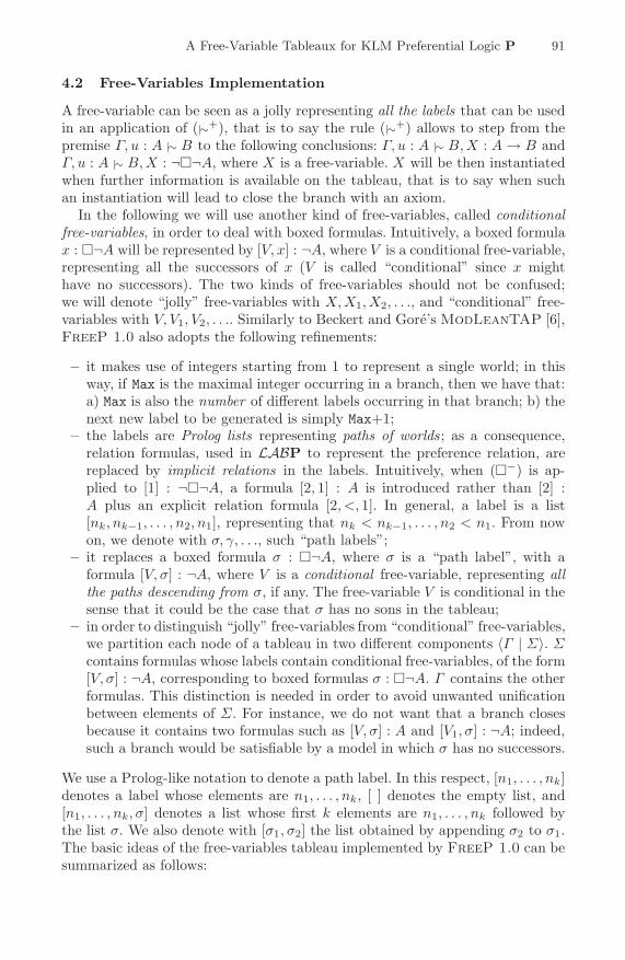
4.2 Free-Variables Implementation

A free-variable can be seen as a jolly representing all the labels that can be usedin an application of (|∼+), that is to say the rule (|∼+) allows to step from thepremise Γ, u : A |∼ B to the following conclusions: Γ, u : A |∼ B, X : A → B andΓ, u : A |∼ B, X : ¬�¬A, where X is a free-variable. X will be then instantiatedwhen further information is available on the tableau, that is to say when suchan instantiation will lead to close the branch with an axiom.

In the following we will use another kind of free-variables, called conditionalfree-variables, in order to deal with boxed formulas. Intuitively, a boxed formulax : �¬A will be represented by [V, x] : ¬A, where V is a conditional free-variable,representing all the successors of x (V is called “conditional” since x mighthave no successors). The two kinds of free-variables should not be confused;we will denote “jolly” free-variables with X, X1, X2, . . ., and “conditional” free-variables with V, V1, V2, . . .. Similarly to Beckert and Gore’s ModLeanTAP [6],FreeP 1.0 also adopts the following refinements:

– it makes use of integers starting from 1 to represent a single world; in thisway, if Max is the maximal integer occurring in a branch, then we have that:a) Max is also the number of different labels occurring in that branch; b) thenext new label to be generated is simply Max+1;

– the labels are Prolog lists representing paths of worlds ; as a consequence,relation formulas, used in LABP to represent the preference relation, arereplaced by implicit relations in the labels. Intuitively, when (�−) is ap-plied to [1] : ¬�¬A, a formula [2, 1] : A is introduced rather than [2] :A plus an explicit relation formula [2, <, 1]. In general, a label is a list[nk, nk−1, . . . , n2, n1], representing that nk < nk−1, . . . , n2 < n1. From nowon, we denote with σ, γ, . . ., such “path labels”;

– it replaces a boxed formula σ : �¬A, where σ is a “path label”, with aformula [V, σ] : ¬A, where V is a conditional free-variable, representing allthe paths descending from σ, if any. The free-variable V is conditional in thesense that it could be the case that σ has no sons in the tableau;

– in order to distinguish “jolly” free-variables from “conditional” free-variables,we partition each node of a tableau in two different components 〈Γ | Σ〉. Σcontains formulas whose labels contain conditional free-variables, of the form[V, σ] : ¬A, corresponding to boxed formulas σ : �¬A. Γ contains the otherformulas. This distinction is needed in order to avoid unwanted unificationbetween elements of Σ. For instance, we do not want that a branch closesbecause it contains two formulas such as [V, σ] : A and [V1, σ] : ¬A; indeed,such a branch would be satisfiable by a model in which σ has no successors.

We use a Prolog-like notation to denote a path label. In this respect, [n1, . . . , nk]denotes a label whose elements are n1, . . . , nk, [ ] denotes the empty list, and[n1, . . . , nk, σ] denotes a list whose first k elements are n1, . . . , nk followed bythe list σ. We also denote with [σ1, σ2] the list obtained by appending σ2 to σ1.The basic ideas of the free-variables tableau implemented by FreeP 1.0 can besummarized as follows:


– when (|∼+) is applied, a jolly free-variable is introduced in the two con-clusions; the free-variable represents all the labels occurring in the currentbranch, and will be instantiated later, when such an instantiation leads toclose a branch with an axiom;

– when the (�−) rule is applied to 〈Γ, σ : ¬�¬A | Σ〉, then the formula[n, σ] : A is added to Γ , where n is Max+1 and Max is the maximal integeroccurring in the branch, whereas [V, n, σ] : ¬A is added to Σ. The conditionalfree-variable V will then be instantiated to close a branch with an axiom.As an example, if another formula [m, n, σ] : A (or [m2, m1, n, σ] : A) willbe introduced in the branch, then the branch will close since V can beinstantiated with [m] (resp. [m2, m1]);

– given a tableau node 〈Γ | Σ, [V, σ] : ¬A〉, the branch is closed when there isa formula of the form [γ, σ] : A belonging to Γ , where γ is a list of numbers.This machinery is used to perform the propagation of boxed formulas, ratherthan explicitly computing, step by step (when a new world is generated), theset Γ M

x→y. In fact, at the world [γ, σ] reachable from σ, the formula ¬A holdsas the labelled formula [V, σ] : ¬A says that ¬A must hold in all the worldsreachable from σ (and V stands for any path from σ).

Observe that the improved implementation of the tableau for R given in [4]already makes use of jolly free-variables. However, it does not introduce neitherpath labels nor conditional free-variables, thus requiring to explicitly computeΓ M

x→y step by step.Coming back to FreeP 1.0, by looking carefully at how free-variables are in-

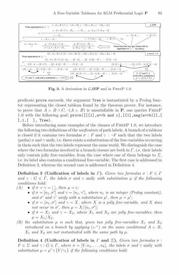
troduced, it can be shown that labels containing jolly free-variables have the form[n1, n2, . . . , nk, X ], where n1, . . . , nk are integers and X is a jolly free-variable.On the contrary, labels containing conditional free-variables have the form [V, σ],where V is a conditional free-variable and σ is a path label that might contain ajolly free-variable. In Figure 3 two derivations of {A |∼ B ∧C, ¬(A |∼ B), ¬(D1 |∼E1), ¬(D2 |∼ E2)} are presented. The upper tableau is obtained by applyingthe simple implementation of LABP introduced in section 4.1, has height 9 andcontains 59 nodes. The lower one, obtained by applying FreeP 1.0, is a tableauof height 6 and contains only 9 nodes.

Here again, the free-variables tableau calculus is implemented by the predi-cate prove( Gamma,Sigma,Max,Cond,Tree), where Gamma and Sigma are Pro-log lists representing a node 〈Γ | Σ〉 as described above and Max is the maximalinteger in the current branch. Cond is used to apply (|∼+) in a controlled way;it is a list whose elements are triples of the form [A=>B,N,Used], representingthat (|∼+) has been applied N times on A |∼ B in the current branch, by in-troducing the free-variables of the list Used. In general, Used is a list of pathspartially instantiated. This machinery is used to control the application of (|∼+)as described in the previous section, in order to ensure termination by prevent-ing that the rule is applied more than once by using the same label. Indeed,as we will see later, the rule is only applied to a conditional A |∼ B if it hasalready been applied less than Max times in the current branch, i.e. N<Max. Fur-thermore, it must be ensured that all labels in Used are different. When the


x : A |∼ B ∧ C, x : ¬(A |∼ B), x : ¬(D1 |∼ E1), x : ¬(D2 |∼ E2). . .

x : A |∼ B ∧ C, v : D2, . . . , z : D1, . . . , y : A, y : �¬A, y : ¬B

v : ¬A, . . . v : ¬�¬A, . . . v : B ∧ C, . . .

z : ¬A, v : ¬A . . . z : ¬�¬A, v : ¬A . . . z : B ∧ C, v : ¬A . . .

y : ¬A, y : A, . . . y : ¬�¬A, y : �¬A, . . .

w < y, w : A,w : ¬A, . . .

y : B ∧ C, y : ¬B, . . .

y : B, y : C, y : ¬B, . . .×

× ×These branches are also closed with an

application of by using y

(|∼−)Three applications of

(|∼+)

(|∼+)

(|∼+)

(|∼+)

. . .

〈[1] : A |∼ B ∧ C, [4] : D2, . . . , [3] : D1, . . . , [2] : A, [2] : ¬B | . . . , [V, 2] : ¬A〉

〈[1] : A |∼ B ∧ C, [1] : ¬(A |∼ B), [1] : ¬(D1 |∼ E1), [1] : ¬(D2 |∼ E2) | ∅〉

〈[X] : A → (B ∧ C), . . . , [2] : A, [2] : ¬B | . . . , [V, 2] : ¬A〉

〈[X] : ¬A, . . . , [2] : A, [2] : ¬B | . . . , [V, 2] : ¬A〉〈[X] : B ∧ C, . . . , [2] : A, [2] : ¬B | . . . , [V, 2] : ¬A〉

(|∼−)Three applications of

(|∼+)

〈[X] : B, [X] : C, . . . , [2] : A, [2] : ¬B | . . . , [V, 2] : ¬A〉unify with a substitution

〈[5, X] : A, . . . | . . . , [V1, 5, X] : ¬A, [V, 2] : ¬A〉

[X] and [2] µ = {X/2}

×× unify with a substitution

and[5, X] [V, 2]

µ′ = {X/2, V/5}

×(→+)

(∧+)

FreeP 1.0

LABP

Fig. 3. A derivation in LABP and in FreeP 1.0

predicate prove succeeds, the argument Tree is instantiated by a Prolog func-tor representing the closed tableau found by the theorem prover. For instance,to prove that A |∼ B ∧ C, ¬(A |∼ B) is unsatisfiable in P, one queries FreeP

1.0 with the following goal: prove([[[1],a=>b and c],[[1],neg(a=>b)]],[],1,[ ], Tree).

Before introducing some examples of the clauses of FreeP 1.0, we introducethe following two definitions of the unification of path labels. A branch of a tableauis closed if it contains two formulas σ : F and γ : ¬F such that the two labels(paths) σ and γ unify, i.e. there exists a substitution of the free-variables occurringin them such that the two labels represent the same world. We distinguish the casewhere the two formulas involved in a branch closure are both in Γ , i.e. their labelsonly contain jolly free-variables, from the case where one of them belongs to Σ,i.e. its label also contains a conditional free-variable. The first case is addressed inDefinition 3, whereas the second case is addressed in Definition 4.

Definition 3 (Unification of labels in Γ ). Given two formulas σ : F ∈ Γand γ : G ∈ Γ , the labels σ and γ unify with substitution μ if the followingconditions hold:

(A) • if σ = γ = [ ], then μ = ε;• if σ = [n1, σ

′] and γ = [n1, γ′], where n1 is an integer (Prolog constant),

and σ′ and γ′ unify with a substitution μ′, then μ = μ′;• if σ = [n1, σ

′] and γ = X, where X is a jolly free-variable, and X doesnot occur in σ′, then μ = X/[n1, σ

′];• if σ = X1 and γ = X2, where X1 and X2 are jolly free-variables, then

μ = X1/X2.(B) the substitution μ is such that, given two jolly free-variables X1 and X2

introduced on a branch by applying (|∼+) on the same conditional A |∼ B,X1 and X2 are not instantiated with the same path by μ.

Definition 4 (Unification of labels in Γ and Σ). Given two formulas σ :F ∈ Σ and γ : G ∈ Γ , where σ = [V, n1, . . . , nk], the labels σ and γ unify withsubstitution μ = μ′ ◦ {V/γ1} if the following conditions hold:


– one can split γ in two parts, i.e. γ = [γ1, γ2], such that γ1 = ε and γ2 = ε1;– γ2 and [n1, . . . , nk] unify w.r.t. Definition 3 with a substitution μ′.

Here below are the clauses implementing axioms:prove(Gamma, , ,Cond,...):-

member([X,A],Gamma),member([Y,neg A],Gamma),matchList(X,Y),constr(Cond),!.

prove(Gamma,Sigma, ,Cond,...):-member([[V|X],A],Sigma),member([Y,neg A],Gamma),copyFormula([[V|X],A],Fml),split(Y,PrefY,SuffY),V=PrefY,matchList(SuffY,X),constr(Cond),!.

The first clause is applied when two formulas [X,A] and [Y,neg A] belong toGamma. The predicate matchList(X,Y) implements the point (A) of Definition 3,i.e. it checks if there exists a substitution of the jolly free-variables belonging to Xand Y such that these two labels unify. The predicate constr(Cond) implementspoint (B) in Definition 3. This ensures the condition of termination of the proofsearch; indeed, as an effect of the matching between labels, the instantiationof some free-variables could lead to duplicate an item in Used, resulting in aredundant application of (|∼+) on A |∼ B in the same world/label. The predicateconstr avoids this situation.

The second clause checks if a branch can be closed by applying a free-variablesubstitution involving a formula in Sigma, i.e. a formula whose label has theform [V|X], where V is a conditional free-variable. Given a formula [Y,neg A]in Gamma and a formula [[V|X],A] in Sigma, if the two path labels unify, thenthe branch can be closed. The clause implements Definition 4 by means of theauxiliary predicates split,V=PrefY, and matchList. In order to allow furtherinstantiations of the conditional free-variable V in other branches, the predicatecopyFormula makes a new copy the labelled formula [[V|X],A], generating aformula Fml of the form [[V’|X’],A], where V’ is a conditional free-variablewhose instantiation is independent from the instantiation of V.

To search a derivation for a set of formulas, FreeP 1.0 proceeds as follows:first, it checks if there exists an instantiation of the free-variables such that thebranch can be closed, by applying the clauses implementing axioms. Otherwise,the first applicable rule will be chosen. The ordering of the clauses is such thatboolean rules are applied in advance. As another example of clause, here belowis one of the clauses implementing (|∼+). It is worth noticing that the followingclause implements a further refinement of the calculus LABP, namely the (�−)rule is “directly” applied to the conclusion of (|∼+), which is the only rule thatintroduces a negated boxed formula X : ¬�¬A in the branch. In this way,an application of (|∼+) to 〈Γ, σ : A |∼ B | Σ〉 leads to the following conclusions:〈Γ, σ : A |∼ B, X : A → B | Σ〉 and 〈Γ, σ : A |∼ B, [n, X ] : A | [X ′, n, X ] : ¬A, Σ〉.The rule (�−) can then be removed from the calculus.prove(Gamma,Sigma,Max,Cond,...):-

member([Label,A=>B],Gamma),

1 Given the form of labels in Γ , these conditions ensure that γ1 does not containfree-variables.


select([A=>B,NumOfWildCards,PrevWildCards],Cond,NewCond),NumOfWildCards<Max,!,NewWildCards#=NumOfWildCards+1,prove([[[X],A->B]|Gamma],Sigma,Max,[[A=>B,NewWildCards,

[[X]|PrevWildCards]]|NewCond],...),!,N#=Max+1,prove([[[N|[X]],A]|Gamma],[[[ |[N|[X]]],neg A]|DefSigma],N,

[[A=>B,NewWildCards,[[X]|PrevWildCards]]|NewCond],...).If a formula [Label,A=>B] belongs to Gamma, then the above clause is invoked. If(|∼+) has already been applied to A |∼ B in the current branch, then an element[A=>B,NumOfWildCards,PrevWildCards] belongs to Cond: the predicate proveis recursively invoked on the two conclusions of the rule only if the predicateNumOfWildCards<Max succeeds, by preventing that the rule is applied a redun-dant number of times. As mentioned above, this machinery, together with thepredicate constr described above, ensure a terminating proof search.

4.3 Performances of FreeP 1.0

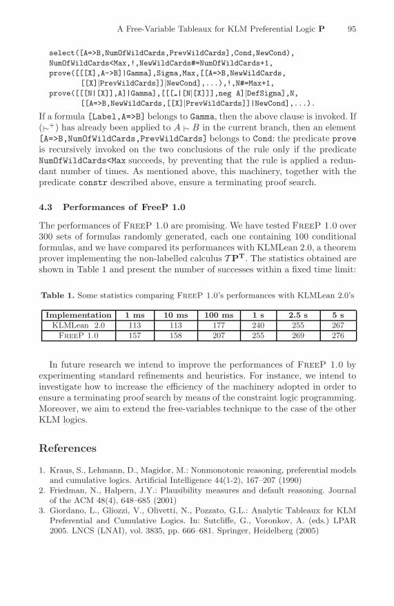
The performances of FreeP 1.0 are promising. We have tested FreeP 1.0 over300 sets of formulas randomly generated, each one containing 100 conditionalformulas, and we have compared its performances with KLMLean 2.0, a theoremprover implementing the non-labelled calculus T PT. The statistics obtained areshown in Table 1 and present the number of successes within a fixed time limit:

Table 1. Some statistics comparing FreeP 1.0’s performances with KLMLean 2.0’s

Implementation 1 ms 10 ms 100 ms 1 s 2.5 s 5 sKLMLean 2.0 113 113 177 240 255 267

FreeP 1.0 157 158 207 255 269 276

In future research we intend to improve the performances of FreeP 1.0 byexperimenting standard refinements and heuristics. For instance, we intend toinvestigate how to increase the efficiency of the machinery adopted in order toensure a terminating proof search by means of the constraint logic programming.Moreover, we aim to extend the free-variables technique to the case of the otherKLM logics.

References

1. Kraus, S., Lehmann, D., Magidor, M.: Nonmonotonic reasoning, preferential modelsand cumulative logics. Artificial Intelligence 44(1-2), 167–207 (1990)

2. Friedman, N., Halpern, J.Y.: Plausibility measures and default reasoning. Journalof the ACM 48(4), 648–685 (2001)

3. Giordano, L., Gliozzi, V., Olivetti, N., Pozzato, G.L.: Analytic Tableaux for KLMPreferential and Cumulative Logics. In: Sutcliffe, G., Voronkov, A. (eds.) LPAR2005. LNCS (LNAI), vol. 3835, pp. 666–681. Springer, Heidelberg (2005)


4. Giordano, L., Gliozzi, V., Pozzato, G.L.: Klmlean 2.0: A theorem prover for KLMLogics of Nonmonotonic Reasoning. In: Olivetti, N. (ed.) TABLEAUX 2007. LNCS(LNAI), vol. 4548, pp. 238–244. Springer, Heidelberg (2007)

5. Fitting, M.: First-Order Logic and Automated Theorem Proving, 2nd edn. (1996)6. Beckert, B., Gore, R.: Free-variable tableaux for propositional modal logics. Studia

Logica 69(1), 59–96 (2001)7. Giordano, L., Gliozzi, V., Olivetti, N., Pozzato, G.L.: Analytic Tableaux Calculi

for KLM Rational Logic R. In: Fisher, M., van der Hoek, W., Konev, B., Lisitsa,A. (eds.) JELIA 2006. LNCS (LNAI), vol. 4160, pp. 190–202. Springer, Heidelberg(2006)

8. Lehmann, D., Magidor, M.: What does a conditional knowledge base entail? Artifi-cial Intelligence 55(1), 1–60 (1992)

An Implementation of a Free-Variable Tableaux for KLM Preferential Logic P of Nonmonotonic Reasoning: The Theorem Prover FreeP 1.0

Documents