No-Hair Theorems and introduction to Hairy Black Holes

1

No-Hair Theorems

and introduction to Hairy Black Holes

By Wahiba Toubal

Submitted on 24/09/2010 in partial fulfilment of the requirements for the degree of

Master of Science of Imperial College London

2

This project has been supervised by Professor Kellogg Stelle.

Abstract

Intensive research on Black holes properties has been carried out in the last 50 years. The

most significant discoveries are the No hair Theorems. Some of these theorems are explained

with a series of proofs. Bekenstein approach is studied as well as a generalised proof by Saa.

A way to avoid these theorems is presented for scalar field hair and SU (N) Einstein Yang

Mill theory with a negative cosmological constant and the MTZ model is introduced.

Introduction

We will start by giving some reminders on general notions used throughout this dissertation.

Reminders on general relativity

Einstein equations are described by

, where is the Ricci tensor,

the Ricci scalar, G the Newtonian constant and the energy-momentum tensor. We

remind the metric for Schwarzschild

.

The electrically charged black holes or the Reissner-Nordstrom black holes are characterised

by the metric [26]. This black hole has a non

zero electromagnetic field which acts as a source of energy-momentum. The energy

momentum tensor for electromagnetism is

where is the

electromagnetic field strength tensor.

Killing Horizon

An asymptotically flat space-time is the one for which the future null infinity, the past null

infinity and the spacelike infinity have the same structure as for Minkowski. The future event

horizon is the surface beyond which timelike curves cannot escape infinity and an analogous

definition holds for the past event horizon.

The most important feature of a black hole is its event horizon. An event horizon is a

hypersurface separating the space-time points that are connected to other space-time points

which are far away from the black hole (far enough to assume that the space-time is described

by Minkowski metric) by a timelike path from the rest. The gradient is normal to the

hypersurface . If the normal vector is null, the hypersurface is said to be null and the normal

3

vector is also tangent to . Null hypersurfaces are considered to be a collection of null

geodesics called the generators of the hypersurface. The tangent vectors to these

geodesics are called and they are proportional to the normal vectors. They also serve as

normal vectors to the hypersurface.[26]

Now if a Killing vector field is null along some null hypersurface we say that is a

Killing horizon of . The vector field is normal to since a null surface cannot have to

linearly independent null tangent vectors.

Event horizon and Killing horizon are closely related in space-times with time translation

symmetry. Every event horizon in a stationary asymptotically flat space-time is a Killing

horizon for some Killing vector field [26].

Soliton

The soliton is an intrinsically non linear solution of the field equation with remarkable

stability and particle like properties. This local travelling wave pulse with a coherent structure

represented a revolution in the non linear science. The soliton is the result of a balance

between two forces: one is linear and acts to disperse the pulse the other has the opposite

effect it is non linear and acts to focus the pulse. Non linearity is essential for balancing the

dispersion process.[9]

Note: throughout the dissertation the prime denotes the partial derivative with respect to the

radial coordinate and the convariant d’Alembertian is

1. The uniqueness theorem

For the no hair theorems, the uniqueness theorem is essential. At the centre of the uniqueness

problem lies the proof that the static electro-vacuum (electrovac) black hole space times (with

no degenerate horizon) are described by the Reissner-Nordstrom (RN) metric, whereas the

circular ones (i.e., the stationary and axisymmetric ones with integrable Killing fields) are

given by the Kerr-Newman metric. A lot of work has been put towards classifying static

black holes in vacuum. The works of Chase, Bekenstein, Hartle and Teitelboim show that

stationary black hole solutions are hairless in a variety of theories where classical fields are

coupled to Einstein gravity. The pioneering investigations in this field were attributed to

Israel, Muller zum Hagen and Robinson. The alternative approach to the problem of the

uniqueness of black hole solutions was proposed by Bunting and Masood-ul-Alam and then

4

strengthened to the Einstein-Maxwell (EM) black holes. Heusler included the magnetically

charged RN solution and static Einstein-σ-model case [28]. The condition of non-

degeneracy of the event horizon was removed and it was shown that Schwarzschild black

hole exhausted the family of all appropriately regular black hole space-times. It was revealed

that RN solution comprised the family of regular black hole space-times under the restrictive

condition that all degenerate components of black hole horizon carried a charge of the same

sign.

In the late sixties, the main contributors to the proof of the uniqueness theorem for the

asymptotically fat, stationary black hole solutions of the Einstein-Maxwell equations were

Israel, Penrose and Wheeler. Using very rigorous proofs, they established that all stationary

electro-vacuum (electrovac) black hole space-times are characterized by their mass, angular

momentum and electric charge This result has a direct implication: all stationary black hole

solutions can be described in terms of a small set of asymptotically measurable quantities. In

the static case it was Israel who, in his pioneering work, was able to establish that both static

vacuum and electrovac black hole space times are spherically symmetric. In particular he

proved in one of his papers that one can consider the limiting external field as a

gravitationally collapsing asymmetric body as static [10]. As a consequence a series of papers

were published showing that the unique non-degenerate electrovac static black hole metrics

are the Reissner-Nordstrom family [11].

It is only in 1989 these statements were disproved when several authors presented a

counterexample within the framework of SU (2) Einstein-Yang-Mills (EYM) theory. The

main argument was to say that although the new solution was static and had vanishing Yang-

Mills charges, it was different from the Schwarzschild black hole and, therefore, not

characterized by its total mass (one of the main reasons the discovery hasn’t happened before

was the belief that EYM equations admit no soliton solutions). Following this discovery a

whole variety of new black hole configurations violating the generalized no-hair conjecture

were found during the last few years. These include, for instance, black holes with Skyrme,

dilaton or Yang-Mills-Higgs hair [8]. As a consequence of the diversity of new solutions, the

different steps of the proof of the uniqueness theorem had to be reconsidered. In particular

questions were asked as to whether there are steps in the uniqueness proof which are not

sensitive to the details of the matter contents.

5

The classical uniqueness theorems were, established for space-times which are either circular

or static. The circularity theorem by Kundt and Trumper and Carter[29] does not hold for the

EYM system unless additional constraints are imposed and the the staticity theorem

establishes the hypersurface orthogonality of the stationary Killing field for electrovac black

hole space times with non-rotating horizons.

The uniqueness theorem for stationary and axisymmetric black holes is mainly based on the

Ernst formulation of the Einstein -Maxwell equations. The key result consists in Carter's

observation that the field equations can be reduced to a 2-dimensional boundary value

problem. An identity due to Robinson then establishes that all vacuum solutions with the

same boundary and regularity conditions are identical [31]. The uniqueness problem for the

electrovac case remained open until Mazur and Bunting independently succeeded in deriving

the desired divergence identities in a systematic way [29].

During the last years the discovery of new black hole solutions in theories with nonlinear

matter fields led scientists to study topics related to the stationary problem of non-rotating

black holes as well as the subject of the stationarity of these objects. Taking into

consideration nonlinear matter models or general sigma models in the present research, the

problems of black hole solutions of the late 1960s and 1970s are reconsidered. Historically

the idea of a staticity theorem was put forward by Lichnerowicz for the simple case in which

there was no black hole. He used the example of a stationary perfect fluid that was

everywhere locally static i.e. its flow vector was aligned with the Killing vector [30]. The

Killing vector itself would have the staticity property of being hypersurface orthogonal.

Hawking extended the research by generalising the proof of staticity to the vacuum case. He

considered black holes that were non-rotating i.e. the null generator of the horizon was

aligned with the Killing vector. Following Hawking contribution, Carter considered an

extension of this problem to the case of electromagnetic fields and obtained the desired result

to some extent. Using the Arnowitt-Deser-Misner (ADM)formalism, Sudarsky and Wald

considered an asymptotically flat solution to Einstein-Yang-Mills (EYM) equations with a

Killing vector field which was timelike at infinity. Using the example of an asymptotically

flat maximal slice with compact interior, they established that the solution is static when it

had a vanishing Yang-Mills electric field on the static hypersurfaces. If an asymptotically flat

solution possesses a black hole, then it is static when it has a vanishing electric field on the

static hypersurface. They also presented a new derivation of the mass formula and proved

that every stationary solution is an extremum of the ADM mass at fixed Yang-Mills electric

6

charge. On the other hand, every stationary black hole solution is an extremum of the ADM

mass at fixed electric charge, canonical angular momentum, and horizon area [27]. One

should also mention the work of Sudarsky and Wald, in which they derived new integral

mass formulas for stationary black holes in EYM theory. Using the notion of maximal

hypersurfaces and combining the mass formulas, they obtained the proof that non-rotating

Einstein-Maxwell (EM) black holes must be static and have a vanishing magnetic field on the

static slices. Hawking's strong rigidity theorem which states that that the event horizon of a

stationary black hole space-time is a Killing horizon represents the basis for the uniqueness

theorem. The theorem establishes a connexion between the event horizon and the Killing

horizon. The theorem requires that the matter fields obey well behaved hyperbolic field

equations and that the stress-energy tensor satisfies the weak energy condition, the theorem

asserts that the event horizon of a stationary black hole space-time is a Killing horizon. This

also implies that either the null-generator Killing field of the horizon coincides with the

stationary Killing field or space-time admits at least one axial Killing field. This theorem

emphasizes that the event horizon of a stationary black hole had to be a Killing horizon; i.e.,

there had to exist a Killing field in the spacetime which was normal to the horizon. If this

field did not coincide with the stationary Killing field then it was shown that the space-

time had to be axisymmetric as well as stationary. It follows that the black hole will be

rotating; i.e., its angular velocity of the horizon will be nonzero ( is defined by the

relation where is an axial Killing vector field) and the Killing vector field

will be spacelike in the vicinity of the horizon. The black hole will be enclosed by an

ergoregion. On the other hand, if coincides with (so that the black hole is non-rotating)

and is globally timelike outside the black hole, then one can show that the spacetime is

static. The standard black hole uniqueness theorem leaves an open question of the problem of

the potential existence of additional stationary black hole solutions of EM equations with a

bifurcate horizon which is neither static nor axisymmetric. The situation was recuperated by

Wald. He showed that any non-rotating black hole in EM theory, the ergoregion of which

was disjoint from the horizon, had to be static, even if the tm was not initially presupposed to

be globally timelike outside the black hole. Chrusciel reconsidered the problem of the strong

rigidity theorem and gave the corrected version of the theorem in which he excluded the

previous assumption about maxi- mal analytic extensions which were not unique [32]. The

uniqueness theorems for black holes are closely related to the problem of staticity. However,

the uniqueness theorems are based on stronger assumptions than the strong rigidity theorem.

7

Namely, in the non-rotating case one requires staticity whereas in the rotating case the

uniqueness theorem is established for circular space-times. The foundations of the uniqueness

theorems were laid by Israel who established the uniqueness of the Schwarzschild metric and

its Reissner-Nordstrom generalization as static asymptotically flat solutions of the Einstein

and EM vacuum field equations. Then, Muller zum Hagen et al. in their works were able to

weaken Israel’s assumptions concerning the topology and regularity of the two-surface

. Robinson generalized the theorem of Israel concerning the

uniqueness of the Schwarzschild black hole. Finally, Bunting and Masood-ul-Alam excluded

multiple black hole solutions, using the conformal transformation and the positive mass

theorem. Lately, a generalization of the results to electro-vacuum space-times was achieved.

The uniqueness results for rotating configurations, i.e., for stationary, axisymmetric black

hole space-times, were obtained by Carter, completed by Hawking and Ellis and the next

works of Carter and Robinson. They were related to the vacuum case. Robinson also gained

a complicated identity which enabled him to expand Carter’s results to electrovac spacetimes.

A quite different approach to the problem under consideration was presented by Bunting and

Mazur. Bunting’s approach was based on applying a general class of harmonic mappings

between Riemannian manifolds while Mazur’s was based on the observation that the Ernst

equations describe a nonlinear s model on symmetric space [33]. A recent review which

covers in detail various aspects of the uniqueness theorems for non-rotating and rotating

black holes was provided by Heusler. Heusler and Straumann considered the stationary EYM

and Einstein dilaton theories. They showed that the mass variation formula involves only

global quantities and surface terms; their results hold for arbitrary gauge groups and any

structure of the Higgs field multiplets. The same authors studied the staticity conjecture and

circularity conditions for rotating black holes in EYM theories. It turned out that contrary to

the Abelian case the staticity conjecture might not hold for non-Abelian gauge fields like the

circularity theorem for these fields. Recently, it has been shown that in the non-Abelian case

stationary black hole space-times with vanishing angular momentum need not to be static

unless they have vanishing electric Yang-Mills charge[28]. Heusler demonstrated that any

self-coupled, stationary scalar mapping (s model! from a domain of strictly outer

communication, with a non-rotating horizon, has to be static. He also proved the no-hair

conjecture for this model.

8

2.No hair theorems:

There are two kinds of no hair theorems in gravitational physics. The first one is the cosmic

non hair theorem which leads to the conclusion that the inflation is a natural phenomenon and

would validate this theory to explain the homogeneity and isotropy of the universe we

observe today [12]. Here we are interested in the black hole no hair theorem.

Historically, a series of no hair theorems appeared when physicists began looking at the

possible interaction of black holes with any kind of matter. Naturally the attention was turned

to scalar fields, which makes the most realistic candidate. The no hair theorems excluded for

a long time scalar fields, vector fields, massive vectors, spinors and Abelian Higgs hair from

stationary black hole exterior. The turning point was the discovery of coloured back holes in

Yang Mils theory and a series of solutions for hairy black holes have been found since then.

Bekenstein was the first one to suggest a no hair theorem but it was quickly proved to be

unstable so we suggested a new one which is the one we are interested in. The statement that

black holes have no hair means that they can only be dressed by field that obey the Gauss law

like the electromagnetic field. Conformal coupling to gravity permitted the discovery of

extremal Reiner Nordstrom geometry because the scalar hair diverges at the horizon; this put

the scalar fields under the no hair theorem.

The presence of a cosmological constant (positive or negative) the Kerr Newman solution to

the Einstein Maxwell equations becomes the Kerr Newman de sitter solution whose space

time is the asymptotically flat the sitter space. The presence of a cosmological constant

changes the asymptotic behaviour and structure of space times. In our example all no hair

theorems have been proves assuming that the space-time is asymptotically flat.

There are different approaches to prove the No Hair Theorems. Scaling arguments provide an

efficient tool for proving nonexistence theorems in at space-time but they are restricted to

highly symmetric situations, this arguments if considered in a more complex way lead to a

first proof of the no-hair theorem for spherically symmetric scalar fields with arbitrary non-

negative potentials. Another proof is based on a mass bound for spherically symmetric black

holes and the circumstance that scalar fields (with harmonic action and non-negative

potentials) violate the strong energy condition [8].

One of the most impressive solutions is the colored black hole solution of the Einstein-Yang-

Mills (EYM) system. Although this solution was found to be unstable in the gravitational

9

sector, non-Abelian hair is generic, and many other non-Abelian black holes were discovered

after the colored black hole.[18]

3. Bekenstein approach:

In his 1995 paper [1] Bekenstein proves the no hair theorem for a black holes dressed with a

multicomponent scalar field. This paper show significant modifications compared to his first

works on no hair theorems. In fact Sudarsky showed that there are some exceptions to the no

hair theorems as first formulated which lead Bekenstein to write a Novel no hair scalar hair

for black holes.

We will follow step by step the proof.

Bekenstein takes the case of a static scalar field in a static black hole background

(1)

Using the action, the field equation is obtained, multiplies by and integrated over the black

hole exterior at a given time. The result obtained is:

(2)

The metric is positive definite with the indices and being spatial coordinates

A theorem states that if is non negative and vanishes only at some discrete values

then the field is constant outside the black hole and its value corresponds to one in the

interval [0, ]. It is particularly the case for Klein Gordon field for which if we consider as

the field’s mass we have . Bechmann and Lechtenfeld objected to Bekhestein

logic and claimed that an exponentially decaying scalar hair can be attached to a static

spherical black hole (BL solution). However in the BL case the potential is not a closed

expression and in some regions the potential is negative which makes it unphysical as it

violates the condition . It is necessary to highlight that the theorem fails for any

field violating the condition for example in the case of the Higgs hair with a

double well potential for which is negative in some regions although some

improvements have been made towards providing proofs of a couple of no-hair theorem for

black holes in the Abelian Higgs model, in arbitrary dimension and for arbitrary horizon

topology [13].

10

For his proof, Bekenstein considers a multiplet of scalar fields in to the following action:

(3)

And from the first derivatives of and , we can form

In nature there are no elementary fields therefore Bekenstein uses the most general form for a

scalar field. He assumes also minimal coupling to gravity and that the energy density carried

by the scalar field is non-negative. The energy momentum tensor corresponding to action in

(3) is :

(4)

The local energy density seen by an observer with four-velocity is:

(5)

Where is an energy density therefore it has to be positive or null. Like for a static black

hole with scalar hair we suppose that the field has a time like killing vector. We can assume

that in Eq. (5) providing the observer moves along the Killing vector .

Therefore, for this specific field we have:

(6)

and this proves the condition that the energy density has to be positive or null. Going back

to Eq. (3), if we take the case when one can see that the terms involving derivatives

dominate . Combining this information with the condition one can conclude that the

dominant terms must be non negative (in our case is a three velocity with which a second

observer moves relative to Killing vector observer. For the case of a free falling frame of

reference co-moving momentarily with the first observer we have , and

where we remind that is the four-velocity). and are

positive provided the conditions below are satisfied:

11

, (7)

(8)

To proceed further, Bekenstein assumes (in the case of a spherically symmetric black hole)

the existence of a self consistent asymptotically flat solution for the Einstein and the scalar

field. In this case the metric outside the horizon can be written as:

(9)

The event horizon radius is at where . This last equation has several

solutions and the horizon always corresponds to the outer zero.

In this proof asymptotic flatness is assumed as well as the non triviality of the scalar field

(this last assumption leads to the conclusion that and depend on ). As a consequence

we have as .

Because of the coordinate invariance of the scalar’s action, the energy momentum tensor

obeys the conservation law:

(10)

A well know result by Landau and Lifshitz shows that the component of Eq. (10) can be

written in the form (the prime here corresponds to the partial derivative with respect to ):

(11)

must be diagonal and

because of the static and spherical symmetry of the

solution we can write Eq (11) as:

(12)

The terms containing the derivative of with respect to cancel and we are left with the

expression:

(13)

12

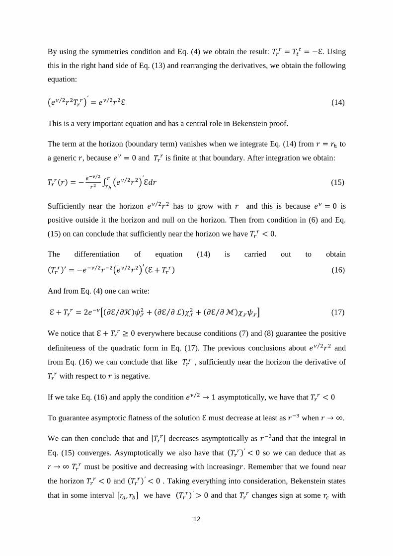
By using the symmetries condition and Eq. (4) we obtain the result:

. Using

this in the right hand side of Eq. (13) and rearranging the derivatives, we obtain the following

equation:

(14)

This is a very important equation and has a central role in Bekenstein proof.

The term at the horizon (boundary term) vanishes when we integrate Eq. (14) from to

a generic , because and is finite at that boundary. After integration we obtain:

(15)

Sufficiently near the horizon has to grow with and this is because is

positive outside it the horizon and null on the horizon. Then from condition in (6) and Eq.

(15) on can conclude that sufficiently near the horizon we have .

The differentiation of equation (14) is carried out to obtain

(16)

And from Eq. (4) one can write:

(17)

We notice that everywhere because conditions (7) and (8) guarantee the positive

definiteness of the quadratic form in Eq. (17). The previous conclusions about and

from Eq. (16) we can conclude that like , sufficiently near the horizon the derivative of

with respect to is negative.

If we take Eq. (16) and apply the condition asymptotically, we have that

To guarantee asymptotic flatness of the solution must decrease at least as when .

We can then conclude that and decreases asymptotically as and that the integral in

Eq. (15) converges. Asymptotically we also have that so we can deduce that as

must be positive and decreasing with increasing . Remember that we found near

the horizon and

. Taking everything into consideration, Bekenstein states

that in some interval we have and that

changes sign at some with

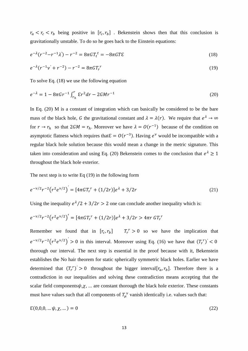
13

being positive in . Bekenstein shows then that this conclusion is

gravitationally unstable. To do so he goes back to the Einstein equations:

(18)

(19)

To solve Eq. (18) we use the following equation

(20)

In Eq. (20) M is a constant of integration which can basically be considered to be the bare

mass of the black hole, the gravitational constant and . We require that

for so that . Moreover we have because of the condition on

asymptotic flatness which requires that . Having would be incompatible with a

regular black hole solution because this would mean a change in the metric signature. This

taken into consideration and using Eq. (20) Bekenstein comes to the conclusion that

throughout the black hole exterior.

The next step is to write Eq (19) in the following form

(21)

Using the inequality one can conclude another inequality which is:

Remember we found that in so we have the implication that

in this interval. Moreover using Eq. (16) we have that

thorough our interval. The next step is essential in the proof because with it, Bekenstein

establishes the No hair theorem for static spherically symmetric black holes. Earlier we have

determined that throughout the bigger interval . Therefore there is a

contradiction in our inequalities and solving these contradiction means accepting that the

scalar field components , , ... are constant thorough the black hole exterior. These constants

must have values such that all components of vanish identically i.e. values such that:

(22)

14

In his argument Bekenstein uses the trivial solution for the scalar equation as a boundary

condition and in order to obtain a trivial solution for the scalar equation in the free empty

space, such values for the scalar field components satisfying Eq. (22) must exist. The

important conclusion that can be made is that the black hole solution must be Schwarchild.

The black hole would have been Reissner-Nordstrom black hole in the case it was electrically

and/or magnetically charged and the scalar fields uncoupled to electromagnetism.

This theorem is very important and lead to several applications. One of them is using a

analogous argument for the Higgs field with an action similar to the one in Eq. (1). To

exclude Higgs hair, we suppose the potential has several wells and we assume the

presence of a global minimum which is . The energy density of the field is positive

definite and we can choose to be one of the values of for which . can serve as

a boundary condition for an asymptotically flat solution which requires that the energy

density vanishes as .but according to the theorem throughout the black holes exterior,

which is sufficient to rule out Higgs hair.

5.Saa approach

In his paper published in 2008 [7] Saa presents a generalisation of Bekenstein method. He

adopts the conventions previously used in [14] to presents a theorem that excludes finite

scalar hairs of any asymptotically flat static and spherically symmetric black hole solution.

However in his paper he doesn’t consider situations where the divergence of the scalar field

is not related to the singularity and where a scalar hair is. The divergence of scalar fields play

an important part in the existence of hairs and this point was further investigated in Zannias

paper [16] considered to exist. To do so he chooses the action

(23)

Where and are positive

In the literature the most common non minimally coupling for the scalar field is

and . The Bekenstein method allows Saa to construct the exact solution from

the solutions of the minimally coupled case. The case

corresponds to the conformal

coupling case and there is also a method to generate solution for arbitrary which is explored

in [15]

He proceeds as follows; he provides a covariant method to provide solutions for our action.

15

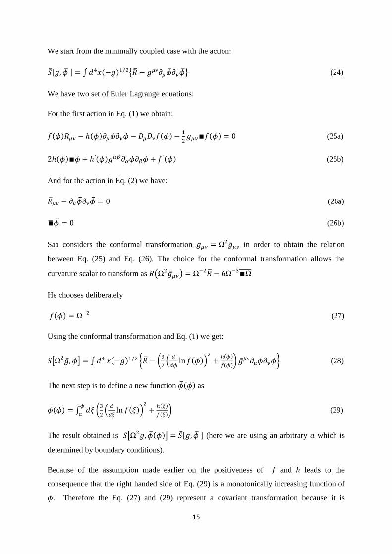
We start from the minimally coupled case with the action:

(24)

We have two set of Euler Lagrange equations:

For the first action in Eq. (1) we obtain:

(25a)

(25b)

And for the action in Eq. (2) we have:

(26a)

(26b)

Saa considers the conformal transformation in order to obtain the relation

between Eq. (25) and Eq. (26). The choice for the conformal transformation allows the

curvature scalar to transform as

He chooses deliberately

(27)

Using the conformal transformation and Eq. (1) we get:

(28)

The next step is to define a new function as

(29)

The result obtained is (here we are using an arbitrary which is

determined by boundary conditions).

Because of the assumption made earlier on the positiveness of and leads to the

consequence that the right handed side of Eq. (29) is a monotonically increasing function of

. Therefore the Eq. (27) and (29) represent a covariant transformation because it is

16

independent of any symmetry assumption and this transformation that maps ( a one-to one

map) a solution of both equations in (25) into a solution of both equations

in (26). If admits a killing vector for which then is also a killing vector

for and this is true because the transformation used also preserves symmetries. This fact

leads us to a very important conclusion for the rest of the proof: if we know all

solutions with a given symmetry we know all with the same symmetry.

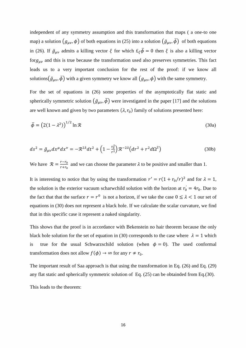
For the set of equations in (26) some properties of the asymptotically flat static and

spherically symmetric solution were investigated in the paper [17] and the solutions

are well known and given by two parameters family of solutions presented here:

(30a)

(30b)

We have

and we can choose the parameter to be positive and smaller than 1.

It is interesting to notice that by using the transformation and for ,

the solution is the exterior vacuum scharwchild solution with the horizon at . Due to

the fact that that the surface is not a horizon, if we take the case our set of

equations in (30) does not represent a black hole. If we calculate the scalar curvature, we find

that in this specific case it represent a naked singularity.

This shows that the proof is in accordance with Bekenstein no hair theorem because the only

black hole solution for the set of equation in (30) corresponds to the case where which

is true for the usual Schwarzschild solution (when ). The used conformal

transformation does not allow for any .

The important result of Saa approach is that using the transformation in Eq. (26) and Eq. (29)

any flat static and spherically symmetric solution of Eq. (25) can be obtainded from Eq.(30).

This leads to the theorem:

17

The only asymptotically flat static and spherically symmetric exterior solution of the system

governed by the action , with the field

finite everywhere is the Shwarchild solution.

6. Solution on black holes in 4D

It has been proven that solution of hairy black holes exists. Most of them are unstable. In this

section we will discuss the different types of hairy black holes and the stability of solution.

We will depart from action which encompasses the characteristics of the system and derive

Einstein and scalar equations from which we will deduce whether the system is stable or not.

18

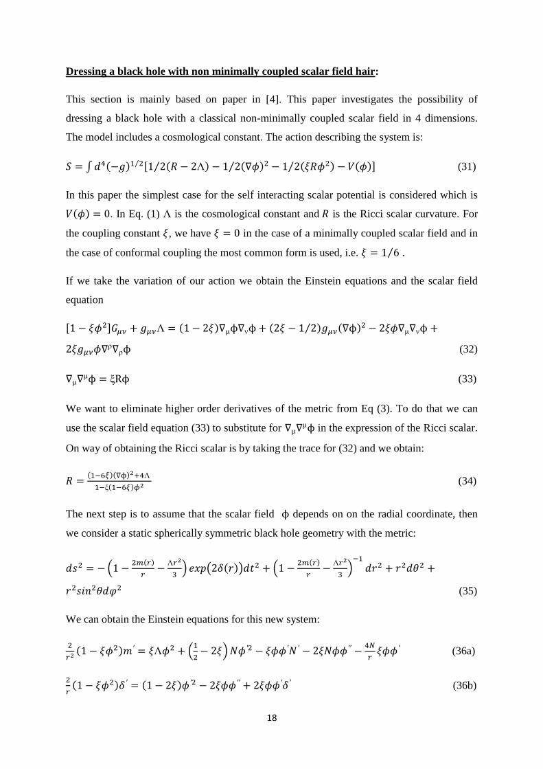
Dressing a black hole with non minimally coupled scalar field hair:

This section is mainly based on paper in [4]. This paper investigates the possibility of

dressing a black hole with a classical non-minimally coupled scalar field in 4 dimensions.

The model includes a cosmological constant. The action describing the system is:

(31)

In this paper the simplest case for the self interacting scalar potential is considered which is

. In Eq. (1) is the cosmological constant and is the Ricci scalar curvature. For

the coupling constant , we have in the case of a minimally coupled scalar field and in

the case of conformal coupling the most common form is used, i.e. .

If we take the variation of our action we obtain the Einstein equations and the scalar field

equation

(32)

(33)

We want to eliminate higher order derivatives of the metric from Eq (3). To do that we can

use the scalar field equation (33) to substitute for in the expression of the Ricci scalar.

On way of obtaining the Ricci scalar is by taking the trace for (32) and we obtain:

(34)

The next step is to assume that the scalar field depends on on the radial coordinate, then

we consider a static spherically symmetric black hole geometry with the metric:

(35)

We can obtain the Einstein equations for this new system:

(36a)

(36b)

19

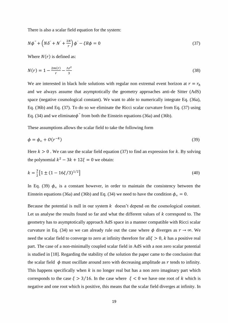
There is also a scalar field equation for the system:

(37)

Where is defined as:

(38)

We are interested in black hole solutions with regular non extremal event horizon at

and we always assume that asymptotically the geometry approaches anti-de Sitter (AdS)

space (negative cosmological constant). We want to able to numerically integrate Eq. (36a),

Eq. (36b) and Eq. (37). To do so we eliminate the Ricci scalar curvature from Eq. (37) using

Eq. (34) and we eliminate from both the Einstein equations (36a) and (36b).

These assumptions allows the scalar field to take the following form

(39)

Here . We can use the scalar field equation (37) to find an expression for . By solving

the polynomial we obtain:

(40)

In Eq. (39) is a constant however, in order to maintain the consistency between the

Einstein equations (36a) and (36b) and Eq. (34) we need to have the condition .

Because the potential is null in our system doesn’t depend on the cosmological constant.

Let us analyse the results found so far and what the different values of correspond to. The

geometry has to asymptotically approach AdS space in a manner compatible with Ricci scalar

curvature in Eq. (34) so we can already rule out the case where diverges as . We

need the scalar field to converge to zero at infinity therefore for all , has a positive real

part. The case of a non-minimally coupled scalar field in AdS with a non zero scalar potential

is studied in [18]. Regarding the stability of the solution the paper came to the conclusion that

the scalar field must oscillate around zero with decreasing amplitude as tends to infinity.

This happens specifically when is no longer real but has a non zero imaginary part which

corresponds to the case . In the case where we have one root of which is

negative and one root which is positive, this means that the scalar field diverges at infinity. In

20

the case the scalar field monotonically decays to zero from its value on the event

horizon.

We want to know how and behave. For , after substituting the expression for

given in Eq. (39) into Einstein equation (36a) we obtain the approximation .

We use the second Einstein equation (36b) to obtain the approximation

therefore with being a constant. It is useful to add that near

we have . Using [19] which studies a similar situation we have

that when the constant is complex and its real part is exactly equal to this

leads to the conclusion that as . Moreover is real when we take the

positive root in Eq.(40) we have . In this case as and

converges to the constant at infinity.

It is well known that stable and non trivial solutions exists when or 1/6. Moreover the

no hair theorem in our system has been proven everywhere in space except when

. It is therefore useful to study the existence and stability of hairy black holes in

this specific case but we will only find the solution for which our conformal transformation is

valid, namely:

(41)

To find these solutions we use a specific method which is presented in [20] for conformally

coupled scalar fields which consists in integrating numerically our minimally coupled field

equations in Eq. (36a) and Eq. (36b) and the solutions are transformed back to the non-

minimally coupled system.

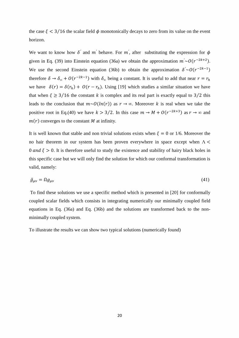
To illustrate the results we can show two typical solutions (numerically found)

21

Figure.1: Examples of typical hairy black-hole solutions with a non-minimally coupled scalar

field, when ξ = 0.1 (dotted) and ξ = 0.2 (solid). For these solutions, the event horizon radius is

taken to be for the ξ = 0.1 solution and for the ξ = 0.2

solution, the cosmological constant and the value of the scalar field at the event

horizon . Solutions for other values of the parameters , , ξ and behave

similarly.

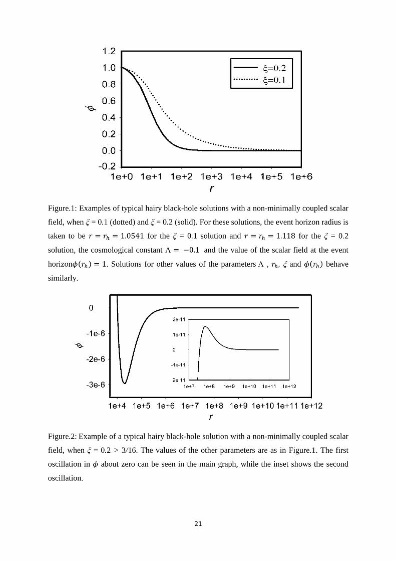
Figure.2: Example of a typical hairy black-hole solution with a non-minimally coupled scalar

field, when ξ = 0.2 > 3/16. The values of the other parameters are as in Figure.1. The first

oscillation in about zero can be seen in the main graph, while the inset shows the second

oscillation.

22

The paper in [21] establishes that many of the black hole solutions in literature are unstable

when subjected to a small perturbation. Let us discuss the stability of our system.

A linear spherically symmetric perturbation of the metric and scalar field is considered. The

perturbation for the scalar field is and following the method used in [19] we can obtain a

perturbation equation for :

The perturbation equation for the system represents a perturbation which is periodic in time

therefore it has the standard Schrödinger form:

(42)

Here is the tortoise coordinate in our asymptotically AdS space. We can choose a specific

value for the constant of integration such that the tortoise coordinate lies in the

interval. and it is related to the radial coordinate by

.

The perturbation potential that we call is given by:

(43)

It vanishes at the event horizon and at infinity it follows the approximation

. For the case the potential remains bounded at infinity. For the

case this means that the potential diverges to positive infinity like as

and diverges to negative infinity like . Now to check the stability we do it

numerically for those solutions with for which the perturbation potential is

positive everywhere outside the vent horizon, we can conclude that the perturbation equation

has no bound state solutions and the black hole is linearly stable.

Now for it is a slightly more complicated case because the potential diverges to

as . The method used is to define a new variable such that and is

positive or null and if we have . The idea is to examine the zero mode solutions

23

of Eq. (42) which are time independent solutions of our perturbation equation. The new

perturbation equation in terms of our new variable can be written as:

(44)

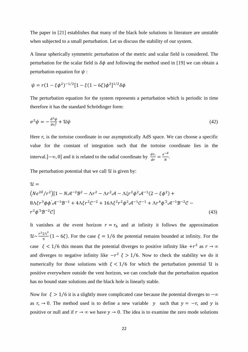
We can show the graph corresponding to the potential in figure 3:

Figure.3: Sketch of the perturbation potential U as a function of y = −r for the black-hole

solutions shown in Figure.1

Now in [22] an important result shows that the number of bound states of the Eq. (44) is

equal to the number of zeros of the zero mode such that . If we define the zero

mode as and impose on it suitable initial conditions at the event horizon we can find zero

modes of the equivalent perturbation equation are found numerically using:

(45)

as we examine the form of the solution of (45) it is a well known result that

behaves like where:

(46)

We are interested in the case because the real part of is positive and as

tends to zero.

24

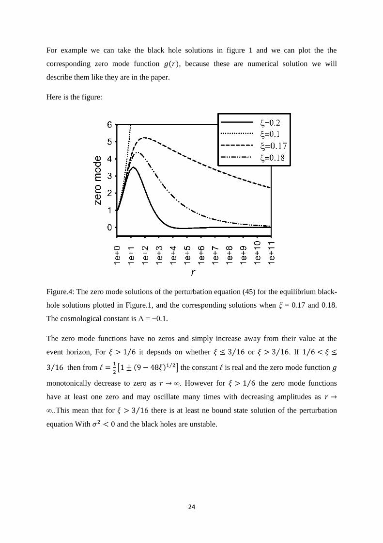
For example we can take the black hole solutions in figure 1 and we can plot the the

corresponding zero mode function , because these are numerical solution we will

describe them like they are in the paper.

Here is the figure:

Figure.4: The zero mode solutions of the perturbation equation (45) for the equilibrium black-

hole solutions plotted in Figure.1, and the corresponding solutions when ξ = 0.17 and 0.18.

The cosmological constant is = −0.1.

The zero mode functions have no zeros and simply increase away from their value at the

event horizon, For it depsnds on whether or . If

then from

the constant is real and the zero mode function

monotonically decrease to zero as . However for the zero mode functions

have at least one zero and may oscillate many times with decreasing amplitudes as

..This mean that for there is at least ne bound state solution of the perturbation

equation With and the black holes are unstable.

25

Hairy black hole solution of Einstein yang mills theory with a negative cosmological

constant.

Over the last years much has been learned about the classical interaction of Yang–Mills fields

with the gravitational field of Einstein’s general relativity. Most investigations have

concentrated on Yang–Mills fields with the gauge group SU (2) starting with Bartnik and

Mckinnon’s discovery of globally regular and asymptotically flat numerical solutions. Their

global existence was analytically proved and many further properties like stability of these

particle-like or Soliton solutions and the corresponding black hole solutions were investigated

numerically as well as analytically. Moreover, many different matter fields can be minimally

coupled to the gravitational and Yang–Mills fields, and corresponding spherically symmetric

solutions have been, mostly numerically, but sometimes also analytically studied.

The proof presented here and based on [4] is a generalisation of black hole solutions of the

SU (2) Einstein –Yang-Mill equations in four dimensional asymptotically flat space-time

found in [3]. The difference between the two paper is that [3] considers topological black

holes too whereas paper in [4] considers only spherically symmetric black holes. In this proof

is the cosmological constant, is the Ricci scalar and the metric signature is .

We are interested in static spherically symmetric Soliton and black hole solutions of the field

equations which are derived by varying the action. This proof is more complex than the ones

given before.

Here we will present the model and the boundary conditions, the solutions are found

numerically and are too complicated to investigate.

For the SU (N) EYM theory the action negative cosmological constant is:

(47)

And the subsequent field equations are:

,

(48)

The YM stress energy tensor is defined by:

(49)

The metric is written in standard Schwarzschild like coordinate and corresponds to:

26

(50)

Like we have seen before, the metric functions and depend on the radial coordinate only

i.e. and . The metric function can be written as:

(51)

According to [23] the most spherically symmetric ansatz for the SU(N) gauge potential is:

(52)

Using a choice of Gauge specified in [23] and because we know that we are only interested in

purely magnetic solutions so we can set and from the beginning but we define

these matrices nonetheless. Matrices and depend only on the radial coordinate and are

purely imaginary traceless diagonal (N N) matices. In Eq. (52) we defined is the

hermitian conjugate to and is a constant (N N) matice defined by

(53)

For the matrix is nilpotent and defined as:

(54)

Where are gauge field functions.

For any if are non zero one of the YM equations becomes

(55)

This is proven in [23] and we will just assume this result here.

A direct consequence is a new expression for the ansatz in Eq. (52) becomes:

(56)

This anzats for the Yang Mills potential is not the only possible one in SU (N) EYM. All

spherically symmetric SU(N) gauge potentials can be found in [26].

The gauge field is described by functions because the only non-zero entries of

the matrix are . The ansatz in Eq. (56) is particularly convenient because we

27

have exactly YM equations for the gauge field functions . .

For our YM fields equation we have:

(57)

With

(58)

And

(59)

In this case, the Einstein equations take the form

and

(60)

and are unknown functions and we have

. As a result we have

ordinary differential equations for unknown functions, , , . For each

independently it is useful to note that the field equations (57) and (60)are invariant under

transformation

(61)

and under the substitution

(62)

The boundary conditions are very important in this proof. Because the cosmological constant

is negative, there is no cosmological horizon. However the field equations are singular at the

origin at the event horizon and at infinity when . Let us briefly present

the boundary conditions.

At the origin

The boundary conditions at the origin are most complicated of the three singular points.

We proceed by assuming that , , have regular Taylor series expansions

(expansions about the singular point about ).

We present the Taylor expansions here:

(63a)

28

(63b)

(63c)

The metric and the curvature are regular at the origin because we impose the condition

(since the metric only involves derivatives of , is otherwise arbitrary) and , ,

are constants.

As a result, the constants and the metric functions are defined as

(64)

and (65)

Because of the invariance of the metric under transformation (61) we can take the positive

root square in Eq. (65). To determine the values of the remaining constants we substitute the

Taylor expansion into the field equations (57) and (60).

At the event horizon:

At where the metric function has a single zero we assume that here is a regular

non extremal event horizon for black hole solutions and this condition fixes the value of

:

(66)

Like for the singular point at the origin we use taylor expansions of the field variables. We

assume that the variables , , have regular Taylor expansions about

(67a)

(67b)

(67c)

We set in (57) and this fixes the derivatives ofthe gauge field functions at

the horizon :

(68)

29

For a fixed cosmological constant the Taylor expansions in (67a), (67b), (67c) are determined

by quantities , , . Without loss of generality we can consider .

At the event horizon we need to have a condition which weakly constrains the values of the

gauge fields functions . Moreover if want the event horizon to be non-extremal we

have to have the condition:

At infinity

As we put a condition on the metric in Eq (50): it has to approaches AdS space-time

the field variables , , converge to constant values.

In a similar way as before we assume that the field variable have Taylor expansion as :

(69a)

(69b)

(69c)

Regarding the values of if the cosmological constant is negative there no constraints on

the values of and the AdS black holes will be magnetically charged. But we can impose

the condition that the space-time is asymptotically flat and with a null cosmological constant

and constrain the values to be

(70)

According to [4] this condition means that these solutions have no global magnetic charge so

at infinity they are indistinguishable from Schwarzschild black holes. At the singular point

which is infinity the fact that the boundary conditions less restrictive when the cosmological

constant is negative leads to the expectation of many more solution in that specific case.

MTZ model

The MTZ black hole, named after Cristian Martinez, Ricardo Troncoso and Jorge Zanelli, is a

black hole solution for (3+1)-dimensional gravity with a conformally coupled self-interacting

30

scalar field The model includes a positive cosmological constant, the space-time is

asymptotically locally AdS and the event horizon is a surface of constant negative curvature.

The advantage of this model is that it reproduces the local propagation properties ok Klein

Gordon field equations on Minkowski space-time better than minimally coupled fields.

Moreover this model allows non trivial black hole solutions.

We will here present the MTZ model and sketched the derivation of two solutions based on

[6]

In this model the action is:

(71)

We have the presence of a scalar field conformally coupled to gravity with and is a

coupling constant, a electromagnetic field and a quatric self-interaction potential. Euler

LaGrange Equations are obtained by varying the action with respect to the scalar field the

Maxwell potential and the metric respectively:

(72a)

(72b)

(72c)

And the stress energy tensors are:

(72d)

(72e)

We deliberately chose a non-minimally coupled scalar field with a quadric self interaction so

that (72a) and (72b) are invariant under conformal transformations of the form a

and and equations and the stress energy tensors transform as

,

under the same transformation.

Identically to the trace of

vanishes on shell

31

(73)

Using the system f equations (72a), (72c), (72d) and (72e) and taking the trace of equation

(72c) we obtain an important relation between the cosmological constant and Ricci scalar:

(74)

In the case where with ( being a constant) we obtain a new system for the

field equations in (72):

(75a)

(75b)

(75c)

These are Einstein equations with an effective Newton constant which given by:

and the case where

is unphysical because it corresponds to

repulsive gravitational forces. This case is further investigated in [25].

Again using (75b) we and taking the trace of (75a) we obtain:

(76)

We notice that using Eq. (76) the Eq. (75b) gives Eq. (74) again and that (75a) takes a

simpler form:

(77)

In this proof, because it seems to admit a wider range of solutions, we are particularly

interested in the case where the coupling constant is tuned with the cosmological constant

as:

(78)

So a distinction can be made between these kind of theories which can be called special

theories where

and the generic theories where

.

32

The field equations for special theories become

(79a)

(79b)

(79c)

In the case . There is an important remark to be made on

because it implies

that . However it doesn’t mean that the gravitational field is unconstrained.

In this paper only static spherically solutions for solutions for the case are explored

and the scalar field depends on the radial coordinate only ( ). The space is defined

by:

(80)

Instead of (72a) we will use a simpler field

(81)

In [25] the exact solution was found to be

(82)

There are two sets of solutions MTZ1 and MTZ2.

The first set of solutions with a constant scalar field

is MTZ1.

By imposing the condition on Eq. (82) we can obtain for generic

theories. For special theories the only constraint on Eq. 982) is Eq. (74)

The conditions in special theories are less restrictive than the ones for generic the theories

therefore we will have a wider set of solutions for special theories.

In fact for for generic theories we have the following set of equations:

and

(83)

33

For special theories we have two integration constants instead of one:

and (84)

In this paper, the singularity at is hiden behind the event horizon because only static

black hole solutions with a sensible stress energy momentum tensor are of interest and we

want

to satisfy the appropriate energy conditions for that. It should be added that these

solution are extremely unstable under perturbation of the metric.

__________________________________________________________________________

34

[1] J.D. Bekenstein, Novel ’no scalar hair’ theorem for black holes, Phys. Rev. D 51 (1995)

6608

[2] Israel W. (1968), Commun. Math. Phys. 8: 245

[3] Radu E 2002 Phys. Lett. B 536 107–13

[4] Elizabeth Winstanley Dressing a black hole with non minimally coupled scalar field hair,

doi: 10.1088/0264-9381/22/11/020

[5] Baxter, Winstanley On the existence of soliton and hairy black hole solutions of SU(N)

Einstein Yang Mill theory with a negative cosmological constant

[6] Martinez C, Troncoso R and Zanelli J 2004 Phys. Rev. D 70 084035

[7] Alberto Saa New no scalar hair for black holes, 10.1063/1.531513

[8] Markus Heusler No hair theorems and black hole with hairs, Institute for Theoretical

Physics The University of Zurich CH8057 Zurich, Switzerland

[9] P.G Drazing, R.S. Johnson, Solitons: An Introduction, Cambridge Texts, 1989

[10] Israel W. (1967), Phys. Rev. 164: 1776

[11] Peter Ruback, A uniqueness theorem for charged black holes, Class. Quantum Grav. 5

(1988) L155-Ll59.

[12]Rong-Gen Cai, Jeong-Young Ji Hair on the cosmological horizon

10.1103/PhysRevD.58.024002

[13]Juan Fernandez-Gracia and Bartomeu Fiol, No-hair theorems for black holes in the

Abelian Higgs model, JHEP11(2009)054 doi: 10.1088/1126-6708/2009/11/054

[14] C.M. Will Theory and experiment in gravitational physics, Cambridge university Press,

1993

[15] A.J. Accioly, U.F. Wichoski, S.F. Kwok, andN.L.P. Pereira da Silva, Class.Quantum

Grav. 10, L215 (1993)

[16] T. Zannias, J Math. Phys 36, 6970 (1995)

35

[17] B.C. Xanthopoulos and T.E. Dialynas, J. Math. Phys. 33, 1463 (1992)

[18] Torii T, Maeda K and Narita M 1999 Phys. Rev. D 59 064027

[19] Henneaux M, Martinez C, Troncoso R and Zanelli J 2004 Phys. Rev. D 70 044034

[20] Winstanley E 2003 Found. Phys. 33 111–43

[21] S. Hod, Phys. Rev. Lett. 100, 121101 (2008); Phys. Rev. D75, 064013 (2007).

[22] Bargmann V 1952 Proc. Natl Acad. Sci. 38 961–6

[23] Kunzle H P 1991 Class. Quantum Grav. 8 2283–97

[24] Bartnik R 1997 J. Math. Phys. 38 3623–38

[25] C. Martinez, R Troncoso and J.Zanelli , Phys rev. D67 024008 (2003)

[26] João Magueijo Advanced General Relativity lecture notes

[27] S.W.Hawking, Comm.Mat.Phys.25, 152 (1972).

[28] M.Heusler, Class.Quantum.Grav.10, 791 (1993).

[29] B.Carter, Phys.Rev.Lett.26, 331 (1971).

[30] A.Lichnerowicz, Theories Relativistes de la Gravitation et de l’Electromagnetism

( Masson, Paris, 1955 ).

[31] D.C.Robinson, Gen.Rel.Grav.8, 695 (1977).

[32] P.T.Chru´sciel, Commun.Math.Phys.bf 189, 1 (1997).

[33] P.O.Mazur, J.Phys.A15, 3173 (1982).

36