New adaptive artificial viscosity method for hyperbolic systems of conservation laws

Page 1

Journal of Computational Physics 231 (2012) 8114–8132

Contents lists available at SciVerse ScienceDirect

Journal of Computational Physics

journal homepage: www.elsevier .com/locate / jcp

New adaptive artificial viscosity method for hyperbolic systemsof conservation laws

Alexander Kurganov, Yu Liu ⇑Mathematics Department, Tulane University, New Orleans, LA 70118, USA

a r t i c l e i n f o

Article history:Received 14 April 2011Received in revised form 1 June 2012Accepted 26 July 2012Available online 14 August 2012

Keywords:Hyperbolic systems of conservation lawsGodunov-type schemesWeak local residualArtificial viscosity

0021-9991/$ - see front matter � 2012 Elsevier Inchttp://dx.doi.org/10.1016/j.jcp.2012.07.040

⇑ Corresponding author.E-mail addresses: [email protected] (A

a b s t r a c t

We propose a new finite volume method for solving general multidimensional hyperbolicsystems of conservation laws. Our method is based on an appropriate numerical flux and ahigh-order piecewise polynomial reconstruction. The latter is utilized without any compu-tationally expensive nonlinear limiters, which are typically needed to guarantee nonlinearstability of the scheme. Instead, we enforce stability of the proposed method by adding anew adaptive artificial viscosity, whose coefficients are proportional to the size of the weaklocal residual, which is sufficiently large (�D, where D is a discrete small scale) at the shockregions, much smaller (�Da , where a is close to 2) near the contact waves, and very small(�D4) in the smooth parts of the computed solution.

We test the proposed scheme on a number of benchmarks for both scalar conservationlaws and for one- and two-dimensional Euler equations of gas dynamics. The obtainednumerical results clearly demonstrate the robustness and high accuracy of the newmethod.

� 2012 Elsevier Inc. All rights reserved.

1. Introduction

We study finite volume Godunov-type schemes for one-dimensional (1-D),

ut þ fðuÞx ¼ 0 ð1:1Þ

and two-dimensional (2-D),

ut þ fðuÞx þ gðuÞy ¼ 0; ð1:2Þ

hyperbolic systems of conservation laws. In the above formulae, u 2 RN is a vector of conserved quantities and fðuÞ and gðuÞare fluxes (the hyperbolicity of the system is ensured provided the matrix nx@f=@uþ ny@g=@u have N real eigenvalues and Nlinearly independent corresponding eigenvectors for any ðnx;nyÞT 2 R2).

Godunov-type schemes form a class of projection-evolution methods, in which at each time step the computed solution isapproximated by a global piecewise polynomial function (called a reconstruction and is supposed to satisfy conservation,accuracy and non-oscillatory requirements), which is evolved in time (from a current time level to the next one) accordingto the integral form of (1.1) (or (1.2), respectively). The latter is obtained by integrating the studied system of conservationlaws over the space–time control volume of size Dt � Dx (or Dt � Dx� Dy, respectively), where Dt is a small temporal scaleand Dx and Dy are small spatial scales. Depending on the way the control volumes are selected, the class of Godunov-type

. All rights reserved.

. Kurganov), [email protected] (Y. Liu).

Page 2

A. Kurganov, Y. Liu / Journal of Computational Physics 231 (2012) 8114–8132 8115

schemes can be split into two subclasses: upwind schemes (their prototype is the original first-order Godunov scheme [7])and central schemes (whose prototype is the first-order Lax-Friedrichs scheme [5,26]). First-order Godunov-type schemesare obtained using the first-order piecewise constant reconstruction, while their higher-order extensions hinge on replace-ment of the first-order reconstruction with a higher-order one, which consists of either linear, parabolic, cubic or even higherdegree polynomial pieces.

Many of the Godunov-type schemes may be written in a particularly simple semi-discrete form (method of lines), ob-tained by integrating (1.1) ((1.2)) over grid cells of size Dx (Dx� Dy) and replacing the fluxes at the cell interfaces (flux inte-grals along the cell boundaries) by appropriate numerical fluxes. In the 1-D case, a semi-discrete scheme on a uniform gridwith xj :¼ jDx can be written as follows. Let xj�1

2:¼ xj � Dx=2 and the computational domain consists of the cells

Ij :¼ ½xj�12; xjþ1

2�. Then, the cell averages of uðx; tÞ over Ij at time t, denoted by

�ujðtÞ �1Dx

Z xjþ1

2

xj�1

2

uðx; tÞdx

are evolved in time by numerically solving the following system of ODEs:

ddt

�ujðtÞ ¼ �Hjþ1

2ðtÞ �Hj�1

2ðtÞ

Dx; ð1:3Þ

where Hjþ12

is a numerical flux, obtained using the piecewise polynomial approximation, reconstructed at time t using the

available cell averages f�ujðtÞg. In our numerical experiments reported in Section 3, we have used the central-upwind fluxesdeveloped in [20,21] (for completeness, both the 1-D and 2-D central-upwind fluxes are briefly reviewed in Appendixes Aand B). However, we would like to stress that the proposed adaptive artificial viscosity method is not tied to any specificnumerical flux and can be implemented with one’s favorite flux, for which the semi-discrete scheme (1.3) is linearly stable.

It is well-known that the systems (1.1) and (1.2) admit nonsmooth solutions that may contain shocks, contact disconti-nuities and rarefaction waves. Therefore, when such solutions are to be captured, linearly stable methods may develop largespurious oscillations and even blow up. Thus, a good numerical method must be nonlinearly stable. Nonlinear stability ofGodunov-type schemes is typically guaranteed by enforcing non-oscillatory nature of the piecewise polynomial reconstruc-tion with the help of nonlinear limiters. However, such limiters may be very complicated and computationally expensive,especially when a high-order multidimensional scheme is to be designed (see, e.g., [38] and references therein). Alterna-tively, one may use less computationally expensive unlimited reconstructions, while enforcing nonlinear stability by addingartificial viscosity to the PDE system in the regions of discontinuities. Obviously, to ensure consistency of the numericalapproximation, this artificial viscosity must vanish as D! 0, where in the 1-D case, D :¼maxðDt;DxÞ and in the 2-D case,D :¼maxðDt;Dx;DyÞ.

The idea of adding artificial viscosity was first proposed in [45] and since then it was notably adopted in many worksincluding [1,9,10,13–15,17,31,36,41,46] among others. The major difficulty in designing a highly accurate and robust artifi-cial viscosity method is to make sure that a sufficient amount of stabilizing diffusion is added wherever it is needed to ensurestability, while in the rest of the computational domain the diffusion must be either switched off or small enough not to af-fect the high accuracy of the scheme there. At the same time, if the viscosity coefficient is too large in the areas of discon-tinuity, the solution will be overly smeared there. Therefore, to achieve overall high resolution, the viscosity should be addedin an adaptive way using a certain indicator, which should automatically pick rough parts of the computed solution anddetermine the (optimal) amount of viscosity needed to be added there.

In this paper, we propose a new adaptive artificial viscosity method. In our method, the viscosity coefficients are chosento be proportional to the size of the weak local residual (WLR), which was originally developed in [18] and then used in[3,19] as a smoothness indicator (SI) for several adaption algorithms. The key point we use here is that for a convergentnumerical method of formal order r, the WLR is proportional to D near (nonlinear) shocks, while it is much smaller

(� Da;a is close to 2) at (linear) contact waves, and tiny in the smooth parts of the solution (� Dminð4;rþ2Þ). Therefore, the arti-ficial viscosity vanishes as one refines the grid, so that it is consistent with the original hyperbolic equations. Moreover, therate at which the viscosity coefficients decay, allows us to achieve the main goal—to stabilize the solution at shock regionswithout oversmearing contact discontinuities or affecting the high resolution of smooth parts of the computed solution.

The key question one has to address to make the adaptive artificial viscosity method robust is how to select the coeffi-cients of proportionality in such a way that the computed solution is non-oscillatory, but its discontinuous parts are wellresolved, that is, they are not overly smeared. To tune the viscosity coefficients, we adopt the strategy proposed in [10]:for the problem at hand, the coefficients are first adjusted on a very coarse mesh and then used for the high-resolution com-putation on finer meshes.

This paper is organized as follows. In Section 2, we describe the derivation of the modified version of the WLR and use it tointroduce adaptive artificial viscosity into both (1.1) and (1.2). The obtained systems are then to be solved by semi-discreteGodunov-type schemes using unlimited high-order reconstructions, which are described in Appendices A and B togetherwith the central-upwind fluxes that have been used in our numerical experiments. In Section 3, we apply the new adaptiveartificial viscosity method to a number of numerical examples in both 1-D and 2-D. We compare our method with the

Page 3

8116 A. Kurganov, Y. Liu / Journal of Computational Physics 231 (2012) 8114–8132

central-upwind scheme combined with the fifth-order WENO reconstruction [2,37,38]. The obtained results indicate highaccuracy, efficiency and robustness of our new method which seems to outperform the WENO approach.

2. New adaptive artificial viscosity method

Godunov-type schemes are projection-evolution methods, in which the approximate solution, realized by its cell aver-ages, is first projected onto the space of piecewise polynomials, and then the obtained piecewise polynomial interpolantis evolved to the new time level using the integral form of conservation laws.

We will focus on semi-discrete schemes, in which the evolution step is performed with the help of numerical fluxes(many reliable numerical fluxes are available, see, e.g., [6,20,27,38,43]). In our numerical experiments, we have used the cen-tral-upwind fluxes from [20], which are presented in Appendices A and B.

The (formal) order of the scheme depends on the (formal) order of the piecewise polynomial reconstruction (we wouldlike to stress that a high-order reconstruction is typically required to achieve high resolution). To ensure a non-oscillatorynature of the scheme the reconstruction can be made non-oscillatory with the help of a nonlinear limiter. A library of suchlimiters is available [2,6,11,12,16,27–30,32,35,38–40,43,44], however, one must realize that first, in the system case, the useof limiters cannot guarantee the scheme to be oscillation-free, and second, the limiters, especially high-order ones, may beextremely computationally expensive and cumbersome, which would dramatically reduce efficiency of the scheme.

An alternative approach for enforcing stability of the method is to introduce numerical diffusion by adding artificial vis-cosity term to the hyperbolic system. This idea dates back to [45], where a viscosity term was added to the momentum equa-tion so that the solution of the new system satisfies the Rankine–Hugoniot jump condition in the shock region and hasnegligible effect outside the shock layer (see also [1]). The critical question is how to adaptively introduce the right amountof viscosity in the right place. It is quite easy to come up with a reliable strategy in the scalar case. In this paper, we propose anew way of adding artificial viscosity, which applies to both scalar and system cases.

2.1. One-dimensional scheme

We augment the hyperbolic system (1.1) with an adaptive artificial viscosity:

ut þ fðuÞx ¼ CðeðuÞuxÞx; ð2:1Þ

where C is a tunable positive viscosity coefficient and eðuÞ is a nonnegative quantity, whose size is automatically adjusteddepending on the local properties of u. For computed solutions, we will make eðuÞ proportional to the WLR, which is one ofthe key points in the construction of our new method.

We would like to stress that our goal is to derive a powerful, efficient and highly accurate method, which can be appliedas a black-box solver to any hyperbolic systems of conservation laws. Therefore, the artificial diffusion term on the right-hand side (RHS) of (2.1) has a general form. For a particular problem at hand, one can add a different artificial diffusion term,which may be based on a small physical viscosity present in the underlying physical system (for instance, in the case of theEuler equations of gas dynamics, one can add Navier–Stokes type artificial diffusion terms). Advantages and disadvantages ofsuch an approach will be studied in future work.

2.1.1. One-dimensional weak local residuals (WLR)In this section, we derive formulae for the WLRs following the approach from [18]. We first consider the system (1.1) in

the computational domain X � ½0; T� and recall that by definition weak solutions of (1.1) satisfy the integral equation

Eðu;/Þ :¼Z T

t¼0

ZX

uðx; tÞ/tðx; tÞ þ fðuðx; tÞÞ/xðx; tÞf gdxdt þZ

Xuðx;0Þ/ðx;0Þdx ¼ 0 ð2:2Þ

for all test functions /ðx; tÞ 2 C10ðX � ½0; TÞÞ. We then assume that the point values of the computed solution un

jþ12

are available

throughout the domain X � ½0; T� and introduce the function uDðx; tÞ as a piecewise constant approximation of the computedsolution by setting

uDðx; tÞ :¼ unjþ1

2; if ðx; tÞ 2 ½xj; xjþ1Þ � ½tn�1

2; tnþ12Þ: ð2:3Þ

The quantity EðuD;/Þ can then be viewed as a weak residual for uD with respect to /. Obviously, the residual (2.3) cannot becomputed in practice since / is a general test function. However, following the approach in [3,18,21], one can approximate

the global test function / with the help of localized test functions /n�1

2

jþ12

and then introduce the corresponding WLRs.

In this paper, we use

/n�1

2jþ1

2ðx; tÞ ¼ Bjþ1

2ðxÞBn�1

2ðtÞ; ð2:4Þ

where

Page 4

A. Kurganov, Y. Liu / Journal of Computational Physics 231 (2012) 8114–8132 8117

Bjþ12ðxÞ :¼

12

x�xj�1Dx

� �2; if xj�1 6 x < xj;

34�

x�xjþ1

2Dx

� �2

; if xj 6 x < xjþ1;

12

x�xjþ2Dx

� �2; if xjþ1 6 x < xjþ2;

0; otherwise

8>>>>>>><>>>>>>>:ð2:5Þ

and

Bn�12ðtÞ :¼

t�tn�32

Dt ; if tn�32 6 t < tn�1

2;

tnþ12�t

Dt ; if tn�12 6 t < tnþ1

2;

0; otherwise

8>><>>: ð2:6Þ

are the quadratic and linear B-splines with the localized supports of size jsupp Bjþ12

� �j ¼ 3Dx and jsupp Bn�1

2

� �j ¼ 2Dt, respec-

tively. One can easily show that for every smooth test function / there exist coefficients bn�1

2jþ1

2, which are independent of Dx

and Dt and satisfy

/ðx; tÞ ¼X

j

Xn

bn�1

2jþ1

2/

n�12

jþ12ðx; tÞ þ OðD2Þ: ð2:7Þ

We then substitute (2.3)–(2.6) into (2.2), use (2.7) and after a straightforward calculation obtain

EðuD;/Þ ¼X

j

Xn

bn�1

2jþ1

2En�1

2jþ1

2þOðD4Þ;

where the quantities

En�12

jþ12¼ 1

6un

jþ32� un�1

jþ32þ 4 un

jþ12� un�1

jþ12

� �þ un

j�12� un�1

j�12

h iDxþ 1

4f un

jþ32

� �� f un

j�12

� �þ f un�1

jþ32

� �� f un�1

j�12

� �h iDt ð2:8Þ

can be viewed as WLRs.

Remark 2.1. Notice that since piecewise polynomial reconstructions used to compute point values of finite volumesolutions are generically discontinuous, two (different) point values are available at each cell interface x ¼ xjþ1

2. We can use

either one or their convex combination to compute the WLR in (2.8). In our numerical experiments, we have used the valueon the left-hand side of each cell interface.

One may show (see [3,18,19]) that the size of WLRs is proportional to D near the shock (in poorly resolved) regions, whilein the smooth (highly resolved) parts of the computed solution the WLRs are several orders of magnitude smaller. Moreover,our numerical experiments demonstrate that typically

kEn�12

jþ12k1 �

D; near shock waves;Da; near contact waves; 1 < a 6 2;Dp; in smooth regions;

8><>:

where p ¼ minfr þ 2;4g and r is the formal order of accuracy of a scheme. Here, the upper bound p ¼ 4 is related to the waythe computed solution is extended in (2.3) and to the particular choice of the locally supported test functions /

n�12

jþ12ðx; tÞ used

in the calculation of the WLR.

2.1.2. One-dimensional adaptive artificial viscosity methodLet us assume that at a certain time level t the approximate solution and the WLR values Ejþ1

2are available. We then select

a linearly stable numerical flux Hjþ12

and evolve the solution according to the semi-discrete scheme

ddt

�uj ¼ �Hjþ1

2�Hj�1

2

Dxþ C

ejþ12D�ujþ1

2� ej�1

2D�uj�1

2

ðDxÞ2

!: ð2:9Þ

Here, D�ujþ12

:¼ �ujþ1 � �uj and ejþ12

:¼maxðjEðiÞj�1

2j; jEðiÞ

jþ12j; jEðiÞ

jþ32jÞ, where EðiÞ

jþ12

is the ith component of the vector so that the artificial

viscosity is proportional to the values of the WLR in the vicinity of xjþ12. In principle, one can use any component of the vector

Ejþ12, but some components might be superior depending on a problem at hand. We also notice that here, the quantities

�uj;Hjþ12

and ejþ12

depend on t, but we suppress this dependence for brevity.

Eq. (2.9) represents our new adaptive artificial viscosity method. The viscosity flux Cejþ12D�ujþ1

2=Dx is proportional to the

size of the WLR in the vicinity of xjþ12. This will guarantee that a substantial amount of the numerical viscosity is added to

the ‘‘rough’’, non-smooth parts of the solution only, while in the smooth regions the numerical viscosity is several ordersof magnitude smaller, and thus the high accuracy will not be affected there. Since no limiters are going to be used, the

Page 5

8118 A. Kurganov, Y. Liu / Journal of Computational Physics 231 (2012) 8114–8132

scheme must have enough numerical diffusion in the shock areas to prevent oscillation. This goal will be achieved by aproper choice of the viscosity coefficients C.

In the scalar case, the size of C can be estimated using the following lemma, which makes a direct connection between theamount of numerical diffusion and the total variation of the computed solution.

Lemma 2.1 ([42]). Consider the following three-point scheme written in a viscous form:

�unþ1j ¼ �un

j � kðf njþ1

2� f n

j�12Þ þ 1

2Q n

jþ12D�un

jþ12� Q n

j�12D�un

j�12

� �; k ¼ Dt

Dx; ð2:10Þ

where

f nj�1

2:¼

f ðunj Þ þ f ðun

j�1Þ2

: ð2:11Þ

If Qnjþ1

2satisfies

kf ðun

jþ1Þ � f ðunj Þ

D�unjþ1

2

���������� 6 Q n

jþ126 1 ð2:12Þ

for all j 2 Z and n P 0, then the scheme (2.1) is total variation diminishing (TVD).Let us now apply the forward Euler time discretization to (2.9). This results in the following fully discrete scheme:

�unþ1j ¼ �un

j � k Hnjþ1

2� Hn

j�12

� �þ kC

Dxen

jþ12D�un

jþ12� en

j�12D�un

j�12

� �: ð2:13Þ

Comparing with (2.10) and noticing that Hnjþ1

2is an approximation of f n

jþ12, we may obtain a rough estimate on the size of C. To

this end, we use Lemma 2.1, which suggests that the adaptive artificial viscosity method should be TVD provided the follow-ing condition is satisfied:

kf ðun

jþ1Þ � f ðunj Þ

D�unjþ1

2

���������� 6 2kCen

jþ12

Dx6 1:

Note that by the CFL condition kj f ðunjþ1Þ � f ðun

j Þ� �

=D�unjþ1

2j 6 0:5, hence we set

C ¼ Dx4ken

max; ð2:14Þ

where enmax ¼max

jen

jþ12

n o. This will ensure that near the shock (where en

jþ12� en

max) the amount of artificial viscosity will be

sufficient to stabilize the computed solution. We now examine the sharpness of the estimate (2.14) numerically.Scalar Numerical Example. Consider the 1-D inviscid Burgers’ equation,

ut þu2

2

� �x

¼ 0;

subject to the 2p-periodic boundary conditions and the following initial condition:

uðx;0Þ ¼ sin xþ 2:5:

We apply the adaptive artificial viscosity method to this initial-boundary value problem with C given by (2.14). In Fig. 2.1(upper row), we show the solution computed on four different grids with 50, 200, 400 and 800 grid cells per period at timet ¼ 2. As one can see, the solution seems to converge to the exact one, but the shock is not well-resolved even when 800 cellsare used. We then significantly reduce the numerical diffusion by replacing the ‘‘theoretical’’ coefficient C with a 15 timessmaller one (we now take C ¼ Dx=ð60ken

maxÞ). The obtained results, plotted in Fig. 2.1 (lower row), show a significantimprovement in the resolution of the shock wave without appearance of any spurious oscillations. We conjecture thatthe method remains stable thanks to the numerical diffusion present at central-upwind numerical fluxes, which are—unlikethe centered flux (2.11)–linearly stable and thus require much less additional artificial viscosity to be added to achieve thenonlinear stability.

This example suggests that the ‘‘theoretical’’ bound on C, obtained in (2.14), is not sharp at all and that even in the scalarcase a better strategy should be used for selecting the viscosity coefficient C. To tune it, we adopt the approach proposed in[10]: for the problem at hand, the coefficient C is first adjusted on a very coarse grid (this makes the tuning process compu-tationally inexpensive) and then used for high-resolution computation on finer grids. The tuning is conducted to find thevalue of C, which leads to sharp resolution of the discontinuities without producing large spurious oscillations. Finding anoptimal C may be a very delicate issue. However, our numerical experiments clearly show that the proposed method isnot too sensitive to the selected value of C, which makes our approach quite robust.

Page 6

0 2 4

1.5

2

2.5

3

3.5

x

u"theoretical" C, N=50

0 2 4

1.5

2

2.5

3

3.5

xu

"theoretical" C, N=200

0 2 4

1.5

2

2.5

3

3.5

x

u

"theoretical" C, N=400

0 2 4

1.5

2

2.5

3

3.5

x

u

"theoretical" C, N=800

0 2 4

1.5

2

2.5

3

3.5

x

u

smaller C, N=50

0 2 4

1.5

2

2.5

3

3.5

x

u

smaller C, N=200

0 2 4

1.5

2

2.5

3

3.5

xu

smaller C, N=400

0 2 4

1.5

2

2.5

3

3.5

x

u

smaller C, N=800

Fig. 2.1. Inviscid Burgers’ equation. Numerical solution zoomed at x 2 ½0;4� at time t ¼ 2 with 50, 200, 400 and 800 grid cells per period and either the‘‘theoretical’’ (upper row) or a smaller (lower row) C.

A. Kurganov, Y. Liu / Journal of Computational Physics 231 (2012) 8114–8132 8119

2.2. Two-dimensional scheme

To construct the 2-D adaptive artificial viscosity method, we first extend Eq. (2.1) to the case of two space dimensions:

ut þ fðuÞx þ gðuÞy ¼ C ðeðuÞuxÞx þ ðeðuÞuyÞyh i

; ð2:15Þ

where, as in the 1-D case, C is a tunable positive viscosity coefficient and eðuÞ is a positive quantity, whose size is propor-tional to the WLR, which will be derived in Section 2.2.1.

We would like to emphasize that similarly to the 1-D case, the artificial diffusion added on the RHS of (2.15) has a generalform, which is not tied to any particular application.

2.2.1. Two-dimensional weak local residualsIn this section, we extend the WLR from one to two space dimensions following the approach from [19]. We consider the

system (1.2) in the computational domain X� ½0; T� and recall that by definition weak solutions of (1.2) satisfy the integralequation

Eðu;/Þ :¼Z 1

t¼0

ZX

uðx;y;tÞ/tðx;y;tÞþ fðuðx;y;tÞÞ/xðx;y;tÞþgðuðx;y;tÞÞ/yðx;y;tÞ

dxdydtþZ

X/ðx;y;0Þuðx;y;0Þdxdy¼0

ð2:16Þ

for all test functions /ðx; y; tÞ 2 C10ðX� ½0; TÞÞ. In complete analogy with the 1-D case, we use the piecewise constant function

uDðx; y; tÞ :¼ unjþ1

2;kþ12; if ðx; y; tÞ 2 ½xj; xjþ1Þ � ½yk; ykþ1Þ � ½tn�1

2; tnþ12Þ ð2:17Þ

to approximate the computed solution and define the localized test functions by

/njþ1

2;kþ12ðx; y; tÞ :¼ 1

DBjþ1

2ðxÞBkþ1

2ðyÞBn�1

2ðtÞ: ð2:18Þ

Here, as before, D :¼maxðDt;Dx;DyÞ, the B-splines Bjþ12

and Bn�12 are given by (2.5) and (2.6), respectively, and Bkþ1

2is defined

in a similar way:

Bkþ12ðyÞ :¼

12

y�yk�1Dy

� �2; if yk�1 6 y < yk;

34�

y�ykþ1

2Dy

� �2

; if yk 6 y < ykþ1;

12

y�ykþ2Dy

� �2; if ykþ1 6 y < ykþ2;

0; otherwise;

8>>>>>>>>><>>>>>>>>>:

Page 7

8120 A. Kurganov, Y. Liu / Journal of Computational Physics 231 (2012) 8114–8132

After plugging (2.17) and (2.18) into (2.16), a straightforward calculation yields the 2-D version of the WLR:

En�12

jþ12;kþ

12¼ 1

36DDxDyUn�1

2jþ1

2;kþ12þ 1

12DDyDtF n�1

2jþ1

2;kþ12þ DxDtGn�1

2jþ1

2;kþ12

� �; ð2:19Þ

where

Un�12

jþ12;kþ

12¼ un

jþ32;kþ

32� un�1

jþ32;kþ

32þ un

jþ32;k�

12� un�1

jþ32;k�

12þ un

j�12;kþ

32� un�1

j�12;kþ

32þ un

j�12;k�

12� un�1

j�12;k�

12

h iþ 4 un

jþ32;kþ

12� un�1

jþ32;kþ

12þ un

j�12;kþ

12� un�1

j�12;kþ

12þ un

jþ12;kþ

32� un�1

jþ12;kþ

32þ un

jþ12;k�

12� un�1

jþ12;k�

12

h iþ 16 un

jþ12;kþ

12� un�1

jþ12;kþ

12

h i;

F n�12

jþ12;kþ

12¼ f un

jþ32;kþ

32

� �� f un

j�12;kþ

32

� �þ f un

jþ32;k�

12

� �� f un

j�12;k�

12

� �þ f un�1

jþ32;kþ

32

� �� f un�1

j�12;kþ

32

� �þ f un�1

jþ32;k�

12

� �� f un�1

j�12;k�

12

� �h iþ 4 f un

jþ32;kþ

12

� �� f un

j�12;kþ

12

� �þ f un�1

jþ32;kþ

12

� �� f un�1

j�12;kþ

12

� �h i

and

Gn�12

jþ12;kþ

12¼ g un

jþ32;kþ

32

� �� g un

jþ32;k�

12

� �þ g un

j�12;kþ

32

� �� g un

j�12;k�

12

� �þ g un�1

jþ32;kþ

32

� �� g un�1

jþ32;k�

12

� �þ g un�1

j�12;kþ

32

� �� g un�1

j�12;k�

12

� �h iþ 4 g un

jþ12;kþ

32

� �� g un

jþ12;k�

12

� �þ g un�1

jþ12;kþ

32

� �� g un�1

jþ12;k�

12

� �h i:

Notice that as in the 1-D case, piecewise polynomial reconstructions used to compute point values of finite volume solutionsare typically discontinuous, four (different) point values are available at each cell corner ðxjþ1

2; ykþ1

2Þ. We can use any of these

values or their convex combination to compute the WLR in (2.19). In our numerical experiments, we have used the value inthe northeast corner of cell ðj; kÞ.

It is easy to show (see [19]; notice however that here, we have rescaled the 2-D WLRs by a factor of 1=D) that the size ofWLRs is proportional to D near shocks (in poorly resolved) regions, while in the smooth (highly resolved) parts of the com-puted solution the WLRs are several orders of magnitude smaller. Our numerical experiments indicate that typically

kEn�12

j;k k1 �D; near shock waves;Da; near contact waves; 1 < a 6 2;Dp; in smooth regions;

8><>:

where p ¼minfr þ 2;4g and r is the formal order of accuracy of a scheme.

Remark 2.2. Notice that our 1-D WLR (2.8) is different from the one developed in [18], and the 2-D WLR (2.19) is differentfrom the one proposed in [19] not only by a factor of 1=D. Here, the size of the support of the localized test functions is3Dx� 2Dt (3Dx� 3Dy� 2Dt for 2-D), while the WLRs in [18,19] were obtained using the localized test functions with a larger(3Dx� 3Dt and 3Dx� 3Dy� 3Dt, respectively) support. We would like to point out that the original version of the WLRs areformally more accurate and they can be used in our adaptive artificial viscosity method provided the time step Dt remainsfixed. However, the current version of the WLRs allows one to vary Dt according to the CFL condition and it is thus moreefficient. Also, the use of data from only two time levels instead of the three ones reduces the computational storagerequirements of the method. On the other hand, we have conducted a large number of numerical experiment that clearlyindicate that the difference in the achieved resolution is negligible.

2.2.2. Two-dimensional adaptive artificial viscosity methodIn 2-D, we assume that the approximate solution �uj;k and the WLRs Ejþ1

2;kþ12

are known at certain time level t, and then weevolve the solution according to the 2-D semi-discrete scheme with linearly stable numerical fluxes Hx

jþ12;k

and Hyj;kþ1

2:

ddt

�uj;k ¼ �Hx

jþ12;k�Hx

j�12;k

Dx�

Hyj;kþ1

2�Hy

j;k�12

Dyþ C

exjþ1

2;kD�ujþ1

2;k� ex

j�12;k

D�uj�12;k

ðDxÞ2þ

eyj;kþ1

2D�uj;kþ1

2� ey

j;k�12D�uj;k�1

2

ðDyÞ2

!: ð2:20Þ

Here, C is as before a positive constant to be tuned,

�uj;k �1

DxDy

Z ykþ1

2

yk�1

2

Z xjþ1

2

xj�1

2

uðx; y; tÞdxdy

is a computed cell average, D�ujþ12;k

:¼ �ujþ1;k � �uj;k and D�uj;kþ12

:¼ �uj;kþ1 � �uj;k.

As in the 1-D case, the key idea of the adaptive artificial viscosity method is to take exjþ1

2;kand ey

j;kþ12

to be proportional toWLRs. To guarantee that enough artificial numerical viscosity is applied to rough parts of the solution, we take

Page 8

Table 1L1-erro

h

2/50

2/10

2/20

2/40

A. Kurganov, Y. Liu / Journal of Computational Physics 231 (2012) 8114–8132 8121

exjþ1

2;k¼max

j;kjEðiÞ

j�12;k�

12j; jEðiÞ

jþ12;k�

12j; jEðiÞ

jþ32;k�

12j; jEðiÞ

j�12;kþ

12j; jEðiÞ

jþ12;kþ

12j; jEðiÞ

jþ32;kþ

12j

n o;

eyj;kþ1

2¼max

j;kjEðiÞ

j�12;k�

12j; jEðiÞ

j�12;kþ

12j; jEðiÞ

j�12;kþ

32j; jEðiÞ

jþ12;k�

12j; jEðiÞ

jþ12;kþ

12j; jEðiÞ

jþ12;kþ

32j

n o;

ð2:21Þ

where EðiÞjþ1

2;kþ12

is the ith component of Ejþ12;kþ

12. In general, one can choose any component i to compute ex

jþ12;k

and eyj;kþ1

2in (2.21),

but some components might be superior depending on a problem at hand. One should choose the component that can pickup the discontinuous part of the solution.

Finally, C in (2.20) is a positive viscosity coefficient, which should be selected to control the quality of the computed solu-tion. To optimize the selection of C, we first tune C on a coarse mesh and then use it for finer mesh computations.

Remark 2.3. The resulting ODE systems (2.9) and (2.20) should be solved by a stable and sufficiently accurate ODE solver. Inthe numerical examples reported in Section 3.3, we have used the third-order SSP Runge–Kutta method from [8].

Remark 2.4. Since the formulae (2.8) and (2.19) require the computed solution at both current and previous time levels, theadaptive artificial viscosity method can only be used from the second time step. To obtain a solution at the first time step,one can use a high-resolution method, which is stabilized with the help of a nonlinear limiter.

3. Numerical examples

In this section, we illustrate the performance of our adaptive artificial numerical viscosity method on several 1-D and 2-Dexamples. We use the central-upwind fluxes and unlimited high-order piecewise polynomial reconstructions described inAppendices A and B. We use the first order extrapolation for the boundary. We compare our results with the results obtainedby the same central-upwind fluxes, but with the fifth-order componentwise WENO reconstruction from [2,37,38] and with-out the adaptive artificial viscosity.

In all of the examples below, we have used a uniform spatial mesh with Dx ¼ Dy ¼ h. We use the ghost cell technique toobtain the absorbing boundary conditions needed to solve initial value problems on finite computational domains. All of therequired ghost values have been obtained using the simplest zero-order extrapolation. The CFL number has been taken in therange of 0:45� 0:5. When the equation of gas dynamics are solved, the viscosity coefficients e in (2.9) and (2.20) are com-puted based on the first (density) component of the WLRs. Our choice is motivated by the fact that in the density equationthe flux is simply qu (see equation Eq. (3.1) below) and thus the computational cost of the resulting method is minimized.

The viscosity coefficient C is tuned in every numerical example below according to the strategy described on page 8. Forbrievity of the presentation, the tuning process is shown in Example 3.1 only.

3.1. Convergence test

We use the 2-D transport equation to demonstrate convergence of the proposed adaptive artificial viscosity method. Weconsider the following initial-boundary value problem:

ut þ 2ux þ uy ¼ 0;uðx; y;0Þ ¼ sinðpðxþ yÞÞ þ 1

2 cosð2pðx� yÞÞ;uðx; y; tÞ ¼ uðxþ 2; y; tÞ ¼ uðx; yþ 2; tÞ:

8><>:

We fix the time step to be either Dt ¼ 0:25h or Dt ¼ h2, compute the corresponding numerical solutions at time t ¼ 2 and

measure their L1-errors:

e1 :¼maxj;k

uj;kð2Þ �1

h2

Z ykþ1

2

yk�1

2

Z xjþ1

2

xj�1

2

uðx; y;0Þdxdy

������������:

The results are presented in Table 1. Clearly, if Dt ¼ 0:25h, which corresponds to the CFL number 0:5, the time discreti-zation errors dominate and our adaptive artificial viscosity method exhibits the third-order convergence. When Dt ¼ h2, then

rs and experimental rates of convergence.

Dt (h) e1 Order Dt e1 Order

0.25 1.042E�3 — h2 3.245E�4 —

0 0.25 1.004E�4 3.38 h2 1.026E�5 4.98

0 0.25 1.161E�5 3.11 h2 3.241E�7 4.99

0 0.25 1.421E�6 3.03 h2 1.044E�8 4.96

Page 9

8122 A. Kurganov, Y. Liu / Journal of Computational Physics 231 (2012) 8114–8132

the spatial errors dominate, and the experimental order of convergence increases to the fifth one (even though our 2-D meth-od is formally fourth-order only, see Appendix B).

3.2. One-dimensional Euler equations of gas dynamics

We numerically solve the Euler equations of gas dynamics:

@

@t

qquE

0B@1CAþ @

@x

qu

qu2 þ puðEþ pÞ

0B@1CA ¼ 0: ð3:1Þ

Here, q;u; p and E are the density, the velocity, the pressure and the total energy, respectively. The equation of state isp ¼ ðc� 1Þ � E� 1

2 qu2� �

and we take c ¼ 1:4.

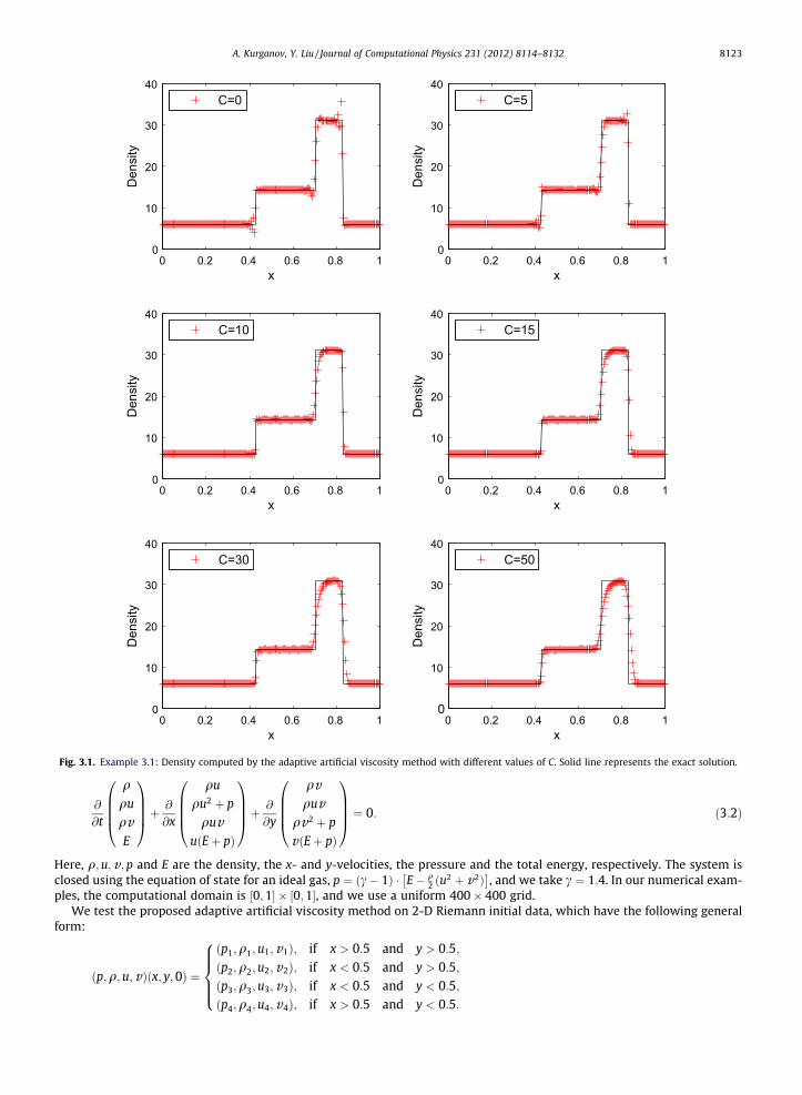
Example 3.1. We solve the Euler Eq. (3.1) subject to the following Riemann initial data [43]:

ðq;u;pÞ ¼ð5:99924;19:5975;460:894Þ; for x < 0:4;ð5:99242;�6:19633;46:0950Þ; for x > 0:4:

�

The exact self-similar solution consists of a left facing shock traveling slowly to the right, a contact wave moving to the right,and a right traveling shock wave. We use our adaptive artificial viscosity method to compute the solution at time t ¼ 0:035with h ¼ 1=200. The obtained results are compared with the exact solution, see [43].

In this example, we take different values of the viscosity coefficient C to demonstrate dependence of the adaptive artificialviscosity method on this parameter. We begin with C ¼ 0. The obtained density is shown on the top left of Fig. 3.1. As one cansee, even though the computed density is very oscillatory, the contact wave is quite sharply resolved. We then increase C andtake C ¼ 5;10;15;30 and 50. From the results, shown in the rest of Fig. 3.1, we may conclude that C ¼ 10 seems to be anoptimal value.

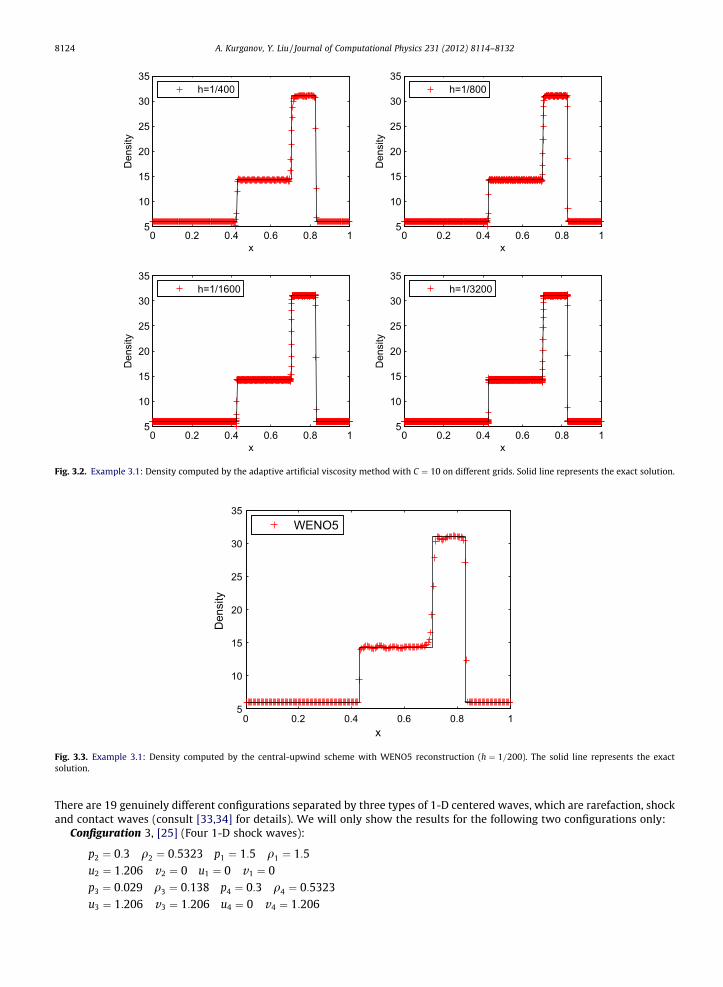
We then verify that C ¼ 10 also works on finer grids. To this end, we refine the mesh to h ¼ 1=400;1=800;1=1600;1=3200and show the obtained results in Fig. 3.2. As one can clearly observe, the numerical solution converges to the exact one.

Finally, we compare our method with the central-upwind scheme with the fifth-order WENO5 reconstruction. The den-sity computed by WENO5 with h ¼ 1=200 is plotted in Fig. 3.3. It seems that our result is as good as the result obtained byWENO5, but our method is less computationally expensive (see Section 3.4).

Example 3.2 (Lax problem, [26]). We numerically solve (3.1) with another set of Riemann initial data:

ðq;u;pÞ ¼ð0:445; 0:698;3:528Þ; for x < 0:5;ð0:5;0;0:571Þ; for x > 0:5:

�

We take h ¼ 1=200 and compute the solution at time t ¼ 0:16 with both the adaptive artificial viscosity method and the cen-tral-upwind scheme with the WENO5 reconstruction.

The density component of the computed solutions is plotted in Fig. 3.4. As one can clearly see, in this example, the adap-tive artificial viscosity method produces a sharper and yet less oscillatory results.

The viscosity coefficient was optimized on a coarse grid and was selected to be C ¼ 45. In Fig. 3.5, we show that this vis-cosity coefficient leads to satisfactory (though a little oscillatory) results on finer meshes as well.

Example 3.3 (Toro’s ‘‘123 problem’’ [43]). In this example, the Riemann initial data are

ðq;u;pÞ ¼ð1:0;�2:0; 0:4Þ; for x < 0:5;ð1:0;2:0;0:4Þ; for x > 0:5:

�

The exact solution consists of two strong symmetric rarefaction waves and a trivial stationary contact discontinuity. Betweenthe two rarefaction waves, the density is very small (close to vacuum), which makes it a suitable test for assessing numericalmethods for low-density flows.

In this example, the central-upwind scheme with the WENO5 reconstruction fails (because of the appearance of negativevalues of computed density and/or pressure), while the adaptive artificial viscosity method performs quite well. We takeh ¼ 1=200; 1=400; 1=800 and 1=1600 and compute the solution at time t ¼ 0:15. As in the previous examples, the viscositycoefficient is tuned on the coarse grid and is taken as C ¼ 15. In Fig. 3.6, one can clearly see that this value of C leads to accu-rate results on finer grids as well.

3.3. Two-dimensional Euler equations of gas dynamics

We now consider the 2-D Euler equations of gas dynamics:

Page 10

0 0.2 0.4 0.6 0.8 10

10

20

30

40

x

Den

sity

C=0

0 0.2 0.4 0.6 0.8 10

10

20

30

40

x

Den

sity

C=5

0 0.2 0.4 0.6 0.8 10

10

20

30

40

x

Den

sity

C=10

0 0.2 0.4 0.6 0.8 10

10

20

30

40

x

Den

sity

C=15

0 0.2 0.4 0.6 0.8 10

10

20

30

40

x

Den

sity

C=30

0 0.2 0.4 0.6 0.8 10

10

20

30

40

x

Den

sity

C=50

Fig. 3.1. Example 3.1: Density computed by the adaptive artificial viscosity method with different values of C. Solid line represents the exact solution.

A. Kurganov, Y. Liu / Journal of Computational Physics 231 (2012) 8114–8132 8123

@

@t

qquqvE

0BBB@1CCCAþ @

@x

qu

qu2 þ pquv

uðEþ pÞ

0BBB@1CCCAþ @

@y

qvquv

qv2 þ p

vðEþ pÞ

0BBB@1CCCA ¼ 0: ð3:2Þ

Here, q;u;v ; p and E are the density, the x- and y-velocities, the pressure and the total energy, respectively. The system isclosed using the equation of state for an ideal gas, p ¼ ðc� 1Þ � E� q

2 ðu2 þ v2Þ�

, and we take c ¼ 1:4. In our numerical exam-ples, the computational domain is ½0;1� � ½0;1�, and we use a uniform 400� 400 grid.

We test the proposed adaptive artificial viscosity method on 2-D Riemann initial data, which have the following generalform:

ðp;q;u; vÞðx; y;0Þ ¼

ðp1;q1;u1;v1Þ; if x > 0:5 and y > 0:5;ðp2;q2;u2;v2Þ; if x < 0:5 and y > 0:5;ðp3;q3;u3;v3Þ; if x < 0:5 and y < 0:5;ðp4;q4;u4;v4Þ; if x > 0:5 and y < 0:5:

8>>><>>>:

Page 11

0 0.2 0.4 0.6 0.8 15

10

15

20

25

30

35

x

Den

sity

h=1/400

0 0.2 0.4 0.6 0.8 15

10

15

20

25

30

35

x

Den

sity

h=1/800

0 0.2 0.4 0.6 0.8 15

10

15

20

25

30

35

x

Den

sity

h=1/1600

0 0.2 0.4 0.6 0.8 15

10

15

20

25

30

35

x

Den

sity

h=1/3200

Fig. 3.2. Example 3.1: Density computed by the adaptive artificial viscosity method with C ¼ 10 on different grids. Solid line represents the exact solution.

0 0.2 0.4 0.6 0.8 15

10

15

20

25

30

35

x

Den

sity

WENO5

Fig. 3.3. Example 3.1: Density computed by the central-upwind scheme with WENO5 reconstruction (h ¼ 1=200). The solid line represents the exactsolution.

8124 A. Kurganov, Y. Liu / Journal of Computational Physics 231 (2012) 8114–8132

There are 19 genuinely different configurations separated by three types of 1-D centered waves, which are rarefaction, shockand contact waves (consult [33,34] for details). We will only show the results for the following two configurations only:

Configuration 3, [25] (Four 1-D shock waves):

p2 ¼ 0:3 q2 ¼ 0:5323 p1 ¼ 1:5 q1 ¼ 1:5u2 ¼ 1:206 v2 ¼ 0 u1 ¼ 0 v1 ¼ 0p3 ¼ 0:029 q3 ¼ 0:138 p4 ¼ 0:3 q4 ¼ 0:5323u3 ¼ 1:206 v3 ¼ 1:206 u4 ¼ 0 v4 ¼ 1:206

Page 12

0 0.2 0.4 0.6 0.8 1

0.4

0.6

0.8

1

1.2

1.4

x

Den

sity

WENO5

0 0.2 0.4 0.6 0.8 1

0.4

0.6

0.8

1

1.2

1.4

x

Den

sity

AAVM

Fig. 3.4. Example 3.2: Density computed by the central-upwind scheme with WENO5 reconstruction, left, and the adaptive artificial viscosity method(AAVM), right. Solid line represents the exact solution.

0 0.2 0.4 0.6 0.8 1

0.4

0.6

0.8

1

1.2

1.4

x

Den

sity

h=1/400

0 0.2 0.4 0.6 0.8 1

0.4

0.6

0.8

1

1.2

1.4

x

Den

sity

h=1/800

Fig. 3.5. Example 3.2: Density computed by the adaptive artificial viscosity method on different grids. Solid line represents the exact solution.

A. Kurganov, Y. Liu / Journal of Computational Physics 231 (2012) 8114–8132 8125

Configuration 19, [25] (One shock, two contacts and one rarefaction wave):

p2 ¼ 1 q2 ¼ 2 p1 ¼ 1 q1 ¼ 1u2 ¼ 0 v2 ¼ �0:3 u1 ¼ 0 v1 ¼ 0:3p3 ¼ 0:4 q3 ¼ 1:0625 p4 ¼ 0:4 q4 ¼ 0:5197u3 ¼ 0 v3 ¼ 0:2145 u4 ¼ 0 v4 ¼ �0:4259

We test the proposed 2-D adaptive artificial viscosity method and compare the obtained results with those computedwith the help of the central-upwind scheme coupled with the 2-D WENO5 reconstruction performed in the dimension-by-dimension manner (see [37] for the reconstruction details).

Figs. 3.7 (Configuration 3) and 3.9 (Configuration 19) show the contour plots of the density (left) and the correspondingvalues of the WLR (right) computed at time t ¼ 0:3 by our adaptive artificial viscosity method. The WENO5 results are shownin Figs. 3.8 and 3.10, respectively. As one can see, the adaptive artificial viscosity method achieves much better resolutionthan the central-upwind scheme with the WENO5 reconstruction. Moreover, our method is more efficient than the WENO5approach (see Section 3.4).

We note that as in the 1-D numerical examples, the viscosity coefficient C was tuned on a coarse grid (with 50� 50 uni-form cells) and was then selected to be equal to 1 (Configuration 3) or 2 (Configuration 19).

3.4. Efficiency test

We now check the efficiency of the adaptive artificial viscosity method by comparing its computational cost with the costof the central-upwind scheme with the fifth-order WENO5 reconstruction.

We first take the 1-D Example 3.1 and run both codes with a fixed spatial grid (Dx ¼ 1=200) and fixed time steps(Dt ¼ Dx=80). The CPU times are 0.227 s for the adaptive artificial viscosity method and 0.542 s for the central-upwindscheme with the WENO5 reconstruction. As one can see, the adaptive artificial viscosity method is about 58:1% faster.

We then proceed with the 2-D Example (Configuration 3 from Section 3.3) and once again use a fixed spatial grid(h ¼ Dx ¼ Dy ¼ 1=200) and fixed time steps (Dt ¼ h=12). The CPU times are 646.974 s for the adaptive artificial viscosity

Page 13

0 0.2 0.4 0.6 0.8 10

0.2

0.4

0.6

0.8

1

1.2

x

Den

sity

h=1/200

0 0.2 0.4 0.6 0.8 10

0.2

0.4

0.6

0.8

1

1.2

x

Den

sity

h=1/400

0 0.2 0.4 0.6 0.8 10

0.2

0.4

0.6

0.8

1

x

Den

sity

h=1/800

0 0.2 0.4 0.6 0.8 10

0.2

0.4

0.6

0.8

1

x

Den

sity

h=1/1600

Fig. 3.6. Example 3.3: Density computed by the adaptive artificial viscosity method with C ¼ 15. Solid line represents the exact solution.

x

y

Density

0.2 0.4 0.6 0.8

0.1

0.2

0.3

0.4

0.5

0.6

0.7

0.8

0.9 0.9

x

y

WLR

0.2 0.4 0.6 0.8

0.1

0.2

0.3

0.4

0.5

0.6

0.7

0.8

Fig. 3.7. Configuration 3: Contour plots (32 contours) of the density computed by the adaptive artificial viscosity method with C ¼ 1 (left) and thecorresponding WLR (right).

8126 A. Kurganov, Y. Liu / Journal of Computational Physics 231 (2012) 8114–8132

method and 1408.503 s for the central-upwind scheme with the WENO5 reconstruction. Thus, in this 2-D example, the adap-tive artificial viscosity method is about 54:1% faster.

We note that the adaptive artificial viscosity method has to be first tested on a coarser grid to optimize the viscosity coef-ficient C, which increases the total computational cost of the adaptive artificial viscosity method. However, if the coarse gridis much coarser than the fine one, the additional computational cost is very small. For instance, in the 2-D case, if the finegrid is with Dx ¼ Dy ¼ 1=400 and the coarse one is with Dx ¼ Dy ¼ 1=50 (as it was the case in the examples brought in Sec-tion 3.3), then each coarse grid experiment will only add about ð1=8Þ3 ¼ 1=512 of the total computational time and say, 10experiments needed to optimize C will only increase the total computational cost of the adaptive artificial viscosity methodby about 2%.

Page 14

WENO5

x

y

0.2 0.4 0.6 0.8

0.1

0.2

0.3

0.4

0.5

0.6

0.7

0.8

0.9

Fig. 3.8. Configuration 3: Contour plot (32 contours) of the density computed by the central-upwind scheme with the WENO5 reconstruction.

Density

x

y

0.2 0.4 0.6 0.8

0.1

0.2

0.3

0.4

0.5

0.6

0.7

0.8

0.9

WLR

x

y

0.2 0.4 0.6 0.8

0.1

0.2

0.3

0.4

0.5

0.6

0.7

0.8

0.9

Fig. 3.9. Configuration 19: Contour plots (29 contours) of the density computed by the adaptive artificial viscosity method with C ¼ 2 (left), and thecorresponding WLR (right).

A. Kurganov, Y. Liu / Journal of Computational Physics 231 (2012) 8114–8132 8127

Appendix A. One-dimensional semi-discrete central-upwind scheme

In this section, we give a brief description of the Godunov-type central-upwind scheme for 1-D hyperbolic systems ofconservation laws (1.1), and we refer readers to [20–22,24] for the derivation of the scheme and more details.

The semi-discrete central-upwind scheme is obtained by using the central-upwind flux,

Hjþ12ðtÞ ¼

aþjþ1

2fðu�

jþ12Þ � a�

jþ12fðuþ

jþ12Þ

aþjþ1

2� aþ

jþ12

þ aþjþ1

2a�jþ1

2

uþjþ1

2� u�

jþ12

aþjþ1

2� a�

jþ12

� qjþ12

" #; ðA:1Þ

Page 15

WENO5

x

y

0.2 0.4 0.6 0.8

0.1

0.2

0.3

0.4

0.5

0.6

0.7

0.8

0.9

Fig. 3.10. Configuration 19: Contour plot (29 contours) of the density computed by the central-upwind scheme with the WENO5 reconstruction.

8128 A. Kurganov, Y. Liu / Journal of Computational Physics 231 (2012) 8114–8132

In (A.1), u�jþ1

2denote the right- and left-sided values of the piecewise polynomial reconstruction euð�; tÞ ¼Pjpjð�; tÞvjð�Þ at

the cell interface x ¼ xjþ12, namely, uþ

jþ12¼ pjþ1ðxjþ1

2Þ and u�

jþ12¼ pjðxjþ1

2Þ. Here, vj is a characteristic function of the cell

Ij ¼ ðxj�12; xjþ1

2Þ and pj are polynomial pieces reconstructed from the cell averages f�ujðtÞg, available at time level t. The recon-

struction, performed in a componentwise manner, must be conservative and sufficiently accurate. In our numerical exam-ples, we have used a fifth-order piecewise polynomial reconstruction consisting of fourth-degree polynomial pieces pjðxÞ,designed to satisfy the following conservation properties:

1Dx

ZIj

pjðxÞdx ¼ �uj;1Dx

ZIj�1

pjðxÞdx ¼ �uj�1;1Dx

ZIj�2

pjðxÞdx ¼ �uj�2:

The one-sided point values of this reconstruction at xjþ12

are

uþjþ1

2¼ 1

60�3�uj�1 þ 27�uj þ 47�ujþ1 � 13�ujþ2 þ 2�ujþ3� �

;

u�jþ12¼ 1

602�uj�2 � 13�uj�1 þ 47�uj þ 27�ujþ1 � 3�ujþ2� �

:

In the case of a convex flux (a central-upwind scheme for the systems with non-convex fluxes was developed in [23]), theone-sided local speeds of propagation used in (A.1) can be estimated by

aþjþ1

2¼max kN

@f@u

u�jþ12

� �� �; kN

@f@u

uþjþ1

2

� �� �; 0

� �;

a�jþ12¼min k1

@f@u

u�jþ12

� �� �; k1

@f@u

uþjþ1

2

� �� �;0

� �;

ðA:2Þ

where, k1 < k2 < � � � < kN are the N eigenvalues of the Jacobian @f@u.

Finally, the built-in anti-diffusion term qjþ1=2 in (A.1) is given by (see [20] for its derivation)

qjþ12¼ 1

aþjþ1

2� a�

jþ12

minmod uþjþ1

2� ujþ1

2;ujþ1

2� u�jþ1

2

� �; ðA:3Þ

where the minmod function, defined as

minmodðz1; z2Þ ¼sgnðz1Þ þ sgnðz2Þ

2minðjz1j; jz2jÞ

Page 16

A. Kurganov, Y. Liu / Journal of Computational Physics 231 (2012) 8114–8132 8129

is applied in (A.3) in a componentwise manner, and the intermediate value ujþ1

2is given by

ujþ12¼

aþjþ1

2uþ

jþ12� a�

jþ12u�

jþ12� f uþ

jþ12

� �� f u�

jþ12

� �n oaþ

jþ12� a�

jþ12

: ðA:4Þ

Remark 3.1. A fully discrete central-upwind scheme will be obtained by solving the ODE system (1.3), (A.1) by a stable ODEsolver of an appropriate order. In the reported numerical examples, we have used the third-order strong stability preservingRunge–Kutta solver ([8]).

Remark 3.2. Notice that the (formal) order of the scheme (1.3), (A.1)–(A.4) depends on the order of the piecewise polyno-mial reconstruction used to evaluate u�

jþ12

and on the order of the ODE solver used to integrate (1.3), see [21,20,22].

Remark 3.3. Note that the quantities u�jþ1

2; pj; a�

jþ12; q�

jþ12

and ujþ1

2used above, depend on t, but we have suppressed this

dependence to simplify the notation.

Appendix B. Two-dimensional semi-discrete central-upwind scheme

In this section, we briefly describe the 2-D semi-discrete central-upwind scheme from [21]. Its derivation and more de-tailed description can be found in [20–22].

Let us consider the 2-D hyperbolic systems of conservation law (1.2) and let �uj;k denote the computed cell averages of u attime t

�uj;k �1

DxDy

Z xjþ1

2

xj�1

2

Z ykþ1

2

yk�1

2

uðx; y; tÞdydx:

The 2-D semi-discrete central-upwind scheme from [21] has the following flux form:

ddt

�uj;kðtÞ ¼ �Hx

jþ12;kðtÞ �Hx

j�12;kðtÞ

Dx�

Hyj;kþ1

2ðtÞ �Hy

j;k�12ðtÞ

Dy; ðB:1Þ

where the fourth-order numerical fluxes are

Hxjþ1

2;kðtÞ : ¼

aþjþ1

2;k

6 aþjþ1

2;k� a�

jþ12;k

� � fðuNEj;k Þ þ 4fðuE

j;kÞ þ fðuSEj;kÞ

h i�

a�jþ1

2;k

6 aþjþ1

2;k� a�

jþ12;k

� � fðuNWjþ1;kÞ þ 4fðuW

jþ1;kÞ þ fðuSWjþ1;kÞ

h i

þaþ

jþ12;k

a�jþ1

2;k

6 aþjþ1

2;k� a�

jþ12;k

� � uNWjþ1;k � uNE

j;k þ 4ðuWjþ1;k � uE

j;kÞ þ uSWjþ1;k � uSE

j;k

h i

and

Hyj;kþ1

2ðtÞ : ¼

bþj;kþ12

6 bþj;kþ12� b�j;kþ1

2

� � gðuNWj;k Þ þ 4gðuN

j;kÞ þ gðuNEj;k Þ

h i�

b�j;kþ12

6 bþj;kþ12� b�j;kþ1

2

� � gðuSWj;kþ1Þ þ 4gðuS

j;kþ1Þ þ gðuSEj;kþ1Þ

h i

þbþj;kþ1

2b�j;kþ1

2

6 bþj;kþ12� b�j;kþ1

2

� � uSWj;kþ1 � uNW

j;k þ 4ðuSj;kþ1 � uN

j;kÞ þ uSEj;kþ1 � uNE

j;k

h i:

Here, uEj;k; uW

j;k; uNj;k; uS

j;k; uNEj;k ; uNW

j;k ; uSEj;k and uSW

j;k are reconstructed point values along the boundary of the cellIj;k :¼ ðxj�1

2; xjþ1

2Þ � ðyk�1

2; ykþ1

2Þ:

uEj;k ¼ euðxjþ1

2; ykÞ; uW

j;k ¼ euðxj�12; ykÞ; uN

j;k ¼ euðxj; ykþ12Þ; uS

j;k ¼ euðxj; yk�12Þ;

uNEj;k ¼ euðxjþ1

2; ykþ1

2Þ; uNW

j;k ¼ euðxj�12; ykþ1

2Þ; uSE

j;k ¼ euðxjþ12; yk�1

2Þ; uSW

j;k ¼ euðxj�12; yk�1

2Þ:

In our numerical experiments, these point values have been obtained using a conservative unlimited fourth-order piecewisepolynomial reconstruction euð�; �; tÞ ¼Pj;kpj;kð�; �; tÞvj;kð�; �Þ, where vj;k is a characteristic function of the cell Ij;k and the 13 coef-ficients (pj;k; ðpxÞj;k; ðpyÞj;k, etc.) of each polynomial piece

Page 17

8130 A. Kurganov, Y. Liu / Journal of Computational Physics 231 (2012) 8114–8132

pj;kðx; yÞ ¼ pj;k þ ðpxÞj;kðx� xjÞ þ ðpyÞj;kðy� ykÞ

þ 12ðpxxÞj;kðx� xjÞ2 þ ðpxyÞj;kðx� xjÞðy� ykÞ þ

12ðpyyÞj;kðy� ykÞ

2

þ 16ðpxxxÞj;kðx� xjÞ3 þ

12ðpxxyÞj;kðx� xjÞ2ðy� ykÞ

þ 12ðpxyyÞj;kðx� xjÞðy� ykÞ

2 þ 16ðpyyyÞj;kðy� ykÞ

3

þ 124ðpxxxxÞj;kðx� xjÞ4 þ

14ðpxxyyÞj;kðx� xjÞ2ðy� ykÞ

2 þ 124ðpyyyyÞj;kðy� ykÞ

4

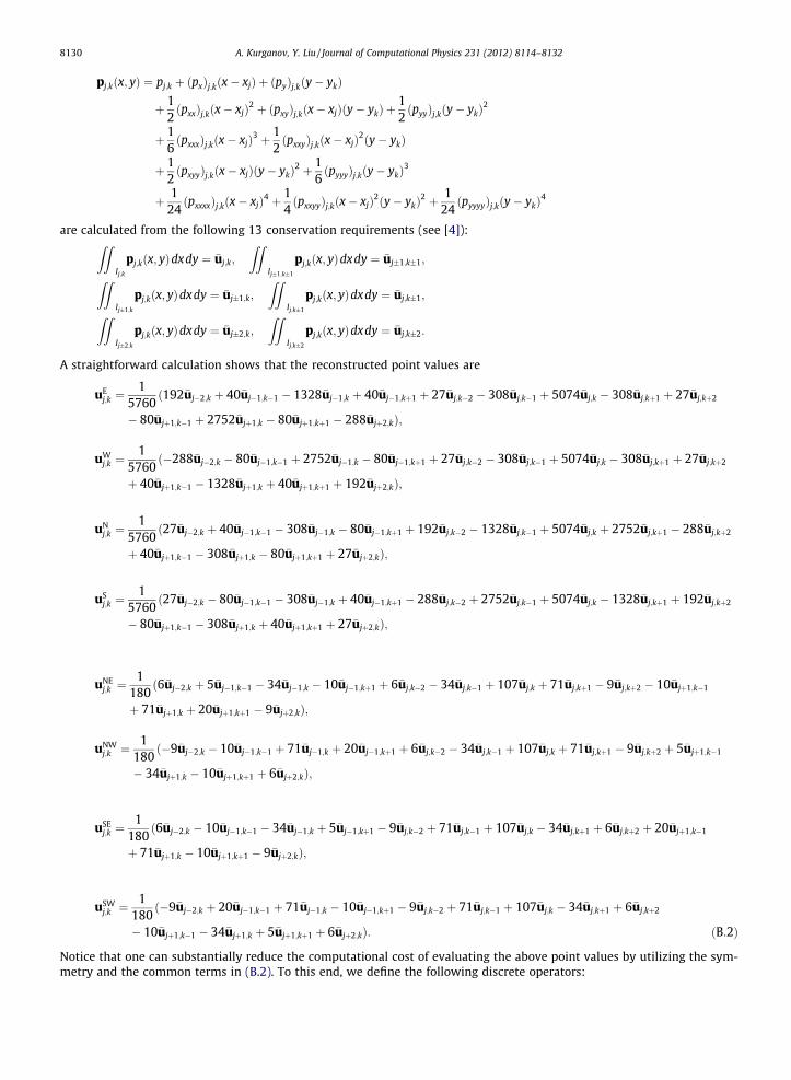
are calculated from the following 13 conservation requirements (see [4]):

ZZIj;k

pj;kðx; yÞdxdy ¼ �uj;k;

ZZIj�1;k�1

pj;kðx; yÞdxdy ¼ �uj�1;k�1;ZZIj�1;k

pj;kðx; yÞdxdy ¼ �uj�1;k;

ZZIj;k�1

pj;kðx; yÞdxdy ¼ �uj;k�1;ZZIj�2;k

pj;kðx; yÞdxdy ¼ �uj�2;k;

ZZIj;k�2

pj;kðx; yÞdxdy ¼ �uj;k�2:

A straightforward calculation shows that the reconstructed point values are

uEj;k ¼

15760

ð192�uj�2;k þ 40�uj�1;k�1 � 1328�uj�1;k þ 40�uj�1;kþ1 þ 27�uj;k�2 � 308�uj;k�1 þ 5074�uj;k � 308�uj;kþ1 þ 27�uj;kþ2

� 80�ujþ1;k�1 þ 2752�ujþ1;k � 80�ujþ1;kþ1 � 288�ujþ2;kÞ;

uWj;k ¼

15760

ð�288�uj�2;k � 80�uj�1;k�1 þ 2752�uj�1;k � 80�uj�1;kþ1 þ 27�uj;k�2 � 308�uj;k�1 þ 5074�uj;k � 308�uj;kþ1 þ 27�uj;kþ2

þ 40�ujþ1;k�1 � 1328�ujþ1;k þ 40�ujþ1;kþ1 þ 192�ujþ2;kÞ;

uNj;k ¼

15760

ð27�uj�2;k þ 40�uj�1;k�1 � 308�uj�1;k � 80�uj�1;kþ1 þ 192�uj;k�2 � 1328�uj;k�1 þ 5074�uj;k þ 2752�uj;kþ1 � 288�uj;kþ2

þ 40�ujþ1;k�1 � 308�ujþ1;k � 80�ujþ1;kþ1 þ 27�ujþ2;kÞ;

uSj;k ¼

15760

ð27�uj�2;k � 80�uj�1;k�1 � 308�uj�1;k þ 40�uj�1;kþ1 � 288�uj;k�2 þ 2752�uj;k�1 þ 5074�uj;k � 1328�uj;kþ1 þ 192�uj;kþ2

� 80�ujþ1;k�1 � 308�ujþ1;k þ 40�ujþ1;kþ1 þ 27�ujþ2;kÞ;

uNEj;k ¼

1180ð6�uj�2;k þ 5�uj�1;k�1 � 34�uj�1;k � 10�uj�1;kþ1 þ 6�uj;k�2 � 34�uj;k�1 þ 107�uj;k þ 71�uj;kþ1 � 9�uj;kþ2 � 10�ujþ1;k�1

þ 71�ujþ1;k þ 20�ujþ1;kþ1 � 9�ujþ2;kÞ;

uNWj;k ¼

1180ð�9�uj�2;k � 10�uj�1;k�1 þ 71�uj�1;k þ 20�uj�1;kþ1 þ 6�uj;k�2 � 34�uj;k�1 þ 107�uj;k þ 71�uj;kþ1 � 9�uj;kþ2 þ 5�ujþ1;k�1

� 34�ujþ1;k � 10�ujþ1;kþ1 þ 6�ujþ2;kÞ;

uSEj;k ¼

1180ð6�uj�2;k � 10�uj�1;k�1 � 34�uj�1;k þ 5�uj�1;kþ1 � 9�uj;k�2 þ 71�uj;k�1 þ 107�uj;k � 34�uj;kþ1 þ 6�uj;kþ2 þ 20�ujþ1;k�1

þ 71�ujþ1;k � 10�ujþ1;kþ1 � 9�ujþ2;kÞ;

uSWj;k ¼

1180ð�9�uj�2;k þ 20�uj�1;k�1 þ 71�uj�1;k � 10�uj�1;kþ1 � 9�uj;k�2 þ 71�uj;k�1 þ 107�uj;k � 34�uj;kþ1 þ 6�uj;kþ2

� 10�ujþ1;k�1 � 34�ujþ1;k þ 5�ujþ1;kþ1 þ 6�ujþ2;kÞ: ðB:2Þ

Notice that one can substantially reduce the computational cost of evaluating the above point values by utilizing the sym-metry and the common terms in (B.2). To this end, we define the following discrete operators:

Page 18

A. Kurganov, Y. Liu / Journal of Computational Physics 231 (2012) 8114–8132 8131

rx1�uj;k :¼ �uj�1;k þ �ujþ1;k; rx

2�uj;k :¼ �uj�2;k þ �ujþ2;k;

ry1�uj;k :¼ �uj;k�1 þ �uj;kþ1; ry

2�uj;k :¼ �uj;k�2 þ �uj;kþ2;

rxy1

�uj;k :¼ rx1�uj;k þ ry

1�uj;k; rxy

2�uj;k :¼ rx

2�uj;k þ ry

2�uj;k;

Dx1�uj;k :¼ �ujþ1;k � �uj�1;k; Dx

2�uj;k :¼ �ujþ2;k � �uj�2;k;

Dy1�uj;k :¼ �uj;kþ1 � �uj;k�1; Dy

2�uj;k :¼ �uj;kþ2 � �uj;k�2;

rd �uj;k :¼ �uj�1;k�1 þ �ujþ1;kþ1 þ �ujþ1;k�1 þ �uj�1;kþ1

ðB:3Þ

and then the following auxiliary quantities, whose dependence on j and k we omit to simplify the notation:

C1 :¼ ð7084�uj;k � 368rxy1

�uj;k þ 27rxy2

�uj;k þ 10rd �uj;kÞ=5760;C2 :¼ ð36Dx

1�uj;k � 5Dx

2�uj;k � Dx

1�uj;kþ1 � Dx

1�uj;k�1Þ=96;

C3 :¼ ð36Dy1�uj;k � 5Dy

2�uj;k � Dy

1�ujþ1;k � Dy

1�uj�1;kÞ=96;

C4 :¼ ð38rx1�uj;k � 3rx

2�uj;k þ 2ry

1�uj;k � rd �uj;k � 70�uj;kÞ=192;

C5 :¼ ð38ry1�uj;k � 3ry

2�uj;k þ 2rx

1�uj;k � rd �uj;k � 70�uj;kÞ=192;

C6 :¼ ðDx1�uj;kþ1 � Dx

1�uj;k�1Þ=16;

C7 :¼ ðDy1�ujþ1;k þ Dy

1�uj�1;k � 2Dx

1�uj;kÞ=32;

C8 :¼ ðDx1�uj;kþ1 þ Dx

1�uj;k�1 � 2Dx

1�uj;kÞ=32;

C9 :¼ ðDx2�uj;k � 2Dx

1�uj;kÞ=96; C10 :¼ ðDy

2�uj;k � 2Dy

1�uj;kÞ=96;

C11 :¼ ð4�uj;k � 2rxy1

�uj;k þ rd �uj;kÞ=64;C12 :¼ ð6�uj;k � 4rx

1�uj;k þ rx

2�uj;kÞ=384; C13 :¼ ð6�uj;k � 4ry

1�uj;k þ ry

2�uj;kÞ=384:

ðB:4Þ

At the end, we rewrite (B.2) as

uEj;k ¼ C1 þ C2 þ C4 þ C9 þ C12;uW

j;k ¼ C1 � C2 þ C4 � C9 þ C12;

uNj;k ¼ C1 þ C3 þ C5 þ C10 þ C13;uS

j;k ¼ C1 � C3 þ C5 � C10 þ C13;

uNEj;k ¼ uE

j;k þ C3 þ C5 þ C6 þ C7 þ C8 þ C10 þ C11 þ C13;

uSEj;k ¼ uE

j;k � C3 þ C5 � C6 � C7 þ C8 � C10 þ C11 þ C13;

uNWj;k ¼ uW

j;k þ C3 þ C5 � C6 þ C7 � C8 þ C10 þ C11 þ C13;

uSWj;k ¼ uW

j;k � C3 þ C5 þ C6 � C7 � C8 � C10 þ C11 þ C13:

ðB:5Þ

Notice that (B.3)–(B.5) is equivalent to (B.2), but the number of multiplications and divisions is now reduced from 112 to 39.Finally, a�

jþ12;k

and b�j;kþ12

are the one-sided local propagation speeds in the x- and y-directions, respectively. In the case ofconvex fluxes, they can be estimated by

aþjþ1

2;k:¼max kN

@f@u

uWjþ1;k

� �� �; kN

@f@u

uEj;k

� �� �; 0

� �;

a�jþ12;k

:¼min k1@f@u

uWjþ1;k

� �� �; k1

@f@u

uEj;k

� �� �; 0

� �;

bþj;kþ12

:¼ max kN@g@u

uSj;kþ1

� �� �; kN

@g@u

uNj;k

� �� �;0

� �;

b�j;kþ12

:¼ min k1@g@u

uSj;kþ1

� �� �; k1

@g@u

uNj;k

� �� �;0

� �;

where k1 < k2 < � � � < kN are the N eigenvalues of the Jacobians @f@u and @g

@u, respectively.

Remark 3.4. A fully discrete 2-D central-upwind scheme can be obtained by solving the ODE system (B.1) with one’s favoriteODE solver. In this paper, we have used the third-order SSP Runge–Kutta solver [8].

Acknowledgement

The work of A. Kurganov was supported in part by the NSF Grant DMS-1115718.

References

[1] E. Caramana, M. Shashkov, P. Whalen, Formulations of artificial viscosity for multi-dimensional shock wave computations, J. Comput. Phys. 144 (1998)70–97.

[2] B. Cockburn, C. Johnson, C.-W. Shu, E. Tadmor, Advanced numerical approximation of nonlinear hyperbolic equations, Lecture Notes in Mathematics,1697, Springer-Verlag, Berlin, 1998.

Page 19

8132 A. Kurganov, Y. Liu / Journal of Computational Physics 231 (2012) 8114–8132

[3] L. Constantin, A. Kurganov, Adaptive central-upwind schemes for hyperbolic systems of conservation laws, in: Hyperbolic Problems: Theory, Numerics,Applications (Osaka, 2004), Yokohama Publishers, 2006, pp. 95–103.

[4] J. Dewar, A. Kurganov, M. Leopold, New residual-based adaption indicator for compressible Euler equations and its application for scheme adaption, inpreparation.

[5] K. Friedrichs, Symmetric hyperbolic linear differential equations, Commun. Pure Appl. Math. 7 (1954) 345–392.[6] E. Godlewski, P.-A. Raviart, Numerical approximation of hyperbolic systems of conservation laws, Applied Mathematical Sciences, 118, Springer-

Verlag, New York, 1996.[7] S. Godunov, A difference method for numerical calculation of discontinuous solutions of the equations of hydrodynamics, Mat. Sb. (N.S.) 47 (89) (1959)

271–306.[8] S. Gottlieb, C.-W. Shu, E. Tadmor, Strong stability-preserving high-order time discretization methods, SIAM Rev. 43 (2001) 89–112 (electronic).[9] J.-L. Guermond, R. Pasquetti, Entropy-based nonlinear viscosity for Fourier approximations of conservation laws, C.R. Math. Acad. Sci. Paris 346 (2008)

801–806.[10] J.-L. Guermond, R. Pasquetti, B. Popov, Entropy viscosity method for nonlinear conservation laws, J. Comput. Phys. 230 (2011) 4248–4267.[11] A. Harten, High resolution schemes for hyperbolic conservation laws, J. Comput. Phys. 49 (1983) 357–393.[12] A. Harten, B. Engquist, S. Osher, S. Chakravarthy, Uniformly high-order accurate essentially nonoscillatory schemes. III, J. Comput. Phys. 71 (1987) 231–

303.[13] R. Hartmann, P. Houston, Adaptive discontinuous Galerkin finite element methods for nonlinear hyperbolic conservation laws, SIAM J. Sci. Comput. 24

(2002) 979–1004 (electronic).[14] R. Hartmann, P. Houston, Adaptive discontinuous Galerkin finite element methods for the compressible Euler equations, J. Comput. Phys. 183 (2002)

508–532.[15] T. Hughes, M. Mallet, A new finite element formulation for computational fluid dynamics. IV. A discontinuity-capturing operator for multidimensional

advective-diffusive systems, Comput. Methods Appl. Mech. Eng. 58 (1986) 329–336.[16] G.-S. Jiang, C.-W. Shu, Efficient implementation of weighted ENO schemes, J. Comput. Phys. 126 (1996) 202–228.[17] C. Johnson, A. Szepessy, P. Hansbo, On the convergence of shock-capturing streamline diffusion finite element methods for hyperbolic conservation

laws, Math. Comput. 54 (1990) 107–129.[18] S. Karni, A. Kurganov, Local error analysis for approximate solutions of hyperbolic conservation laws, Adv. Comput. Math. 22 (2005) 79–99.[19] S. Karni, A. Kurganov, G. Petrova, A smoothness indicator for adaptive algorithms for hyperbolic systems, J. Comput. Phys. 178 (2002) 323–341.[20] A. Kurganov, C.-T. Lin, On the reduction of numerical dissipation in central-upwind schemes, Commun. Comput. Phys. 2 (2007) 141–163.[21] A. Kurganov, S. Noelle, G. Petrova, Semi-discrete central-upwind scheme for hyperbolic conservation laws and Hamilton–Jacobi equations, SIAM J. Sci.

Comput. 23 (2001) 707–740.[22] A. Kurganov, G. Petrova, A third-order semi-discrete genuinely multidimensional central scheme for hyperbolic conservation laws and related

problems, Numer. Math. 88 (2001) 683–729.[23] A. Kurganov, G. Petrova, B. Popov, Adaptive semi-discrete central-upwind schemes for nonconvex hyperbolic conservation laws, SIAM J. Sci. Comput.

29 (2007) 2381–2401.[24] A. Kurganov, E. Tadmor, New high resolution central schemes for nonlinear conservation laws and convection-diffusion equations, J. Comput. Phys. 160

(2000) 241–282.[25] A. Kurganov, E. Tadmor, Solution of two-dimensional riemann problems for gas dynamics without riemann problem solvers, Numer. Methods Partial

Diff. Equat. 18 (2002) 584–608.[26] P. Lax, Weak solutions of nonlinear hyperbolic equations and their numerical computation, Comm. Pure Appl. Math. 7 (1954) 159–193.[27] R. LeVeque, Finite Volume Methods for Hyperbolic Problems, Cambridge Texts in Applied Mathematics, Cambridge University Press, Cambridge, 2002.[28] D. Levy, G. Puppo, G. Russo, Central WENO schemes for hyperbolic systems of conservation laws, M2AN Math, Model. Numer. Anal. 33 (1999) 547–571.[29] D. Levy, G. Puppo, G. Russo, Compact central WENO schemes for multidimensional conservation laws, SIAM J. Sci. Comput. 22 (2000) 656–672

(electronic).[30] X.-D. Liu, S. Osher, T. Chan, Weighted essentially non-oscillatory schemes, J. Comput. Phys. 115 (1994) 200–212.[31] J. Monaghan, R. Gingold, Shock simulation by the particle method SPH, J. Comput. Phys. 52 (1983) 374–389.[32] H. Nessyahu, E. Tadmor, Nonoscillatory central differencing for hyperbolic conservation laws, J. Comput. Phys. 87 (1990) 408–463.[33] C. Schulz-Rinne, Classification of the Riemann problem for two-dimensional gas dynamics, SIAM J. Math. Anal. 24 (1993) 76–88.[34] C. Schulz-Rinne, J. Collins, H. Glaz, Numerical solution of the Riemann problem for two-dimensional gas dynamics, SIAM J. Sci. Comput. 14 (1993)

1394–1414.[35] S. Serna, A. Marquina, Power ENO methods: a fifth-order accurate weighted power ENO method, J. Comput. Phys. 194 (2004) 632–658.[36] A. Shchepetkin, J. McWilliams, Quasi-monotone advection schemes based on explicit locally adaptive dissipation, Month. Weather Rev. 126 (1998)

1541–1580.[37] J. Shi, C. Hu, C.-W. Shu, A technique of treating negative weights in WENO schemes, J. Comput. Phys. 175 (2002) 108–127.[38] C.-W. Shu, High order weighted essentially nonoscillatory schemes for convection dominated problems, SIAM Rev. 51 (2009) 82–126.[39] C.-W. Shu, S. Osher, Efficient implementation of essentially non-oscillatory shock-capturing schemes, J. Comput. Phys. 77 (1988) 439–471.[40] P. Sweby, High resolution schemes using flux limiters for hyperbolic conservation laws, SIAM J. Numer. Anal. 21 (1984) 995–1011.[41] A. Szepessy, Convergence of a shock-capturing streamline diffusion finite element method for a scalar conservation law in two space dimensions,

Math. Comput. 53 (1989) 527–545.[42] E. Tadmor, The large-time behavior of the scalar, genuinely nonlinear Lax-Friedrichs scheme, Math. Comput. 43 (1984) 353–368.[43] E. Toro, Riemann Solvers and Numerical Methods for Fluid Dynamics: A Practical Introduction, third ed., Springer-Verlag, Berlin, Heidelberg, 2009.[44] B. van Leer, Towards the ultimate conservative difference scheme. V. A second-order sequel to Godunov’s method, J. Comput. Phys. 32 (1979) 101–136.[45] J. von Neumann, R. Richtmyer, A method for the numerical calculation of hydrodynamic shocks, J. Appl. Phys. 21 (1950) 232–237.[46] M. Wilkins, Use of artificial viscosity in multidimensional fluid dynamic calculations, J. Comput. Phys. 36 (1980) 281–303.