Neural network: Dynamics of perceptual bistability

Neural network: Dynamics of perceptualbistability

Paul WACRENIER

15 août 2007

Chapitre 1

Experimental study ofperceptual bistability

1.1 introductionWhen an observer experiments an ambiguous stimulus which has two dis-

tincts interpretations, the actual perception alternates over time between thedifferent possible percepts in a random manner. This phenomenon is known asperceptual bi-stability. Bi-stability arises in many type of ambiguous percep-tion : figure ground segregation ( Rubin 1921 , Face/vase illusion), ambiguousfigures (Necker 1832 , Necker cube), ambiguous motion displays (Hupe and Ru-bin 2003, movig plaids), auditory segmentation ( Pressnitzer and Hupe 2006). Moreover the domain of binocular rivalry has been extensively studied ( adifferent image is presented to each eye ), experimentally ( Wheatstone 1838 ;Levelt 1968 ; Blake 1989 ; Logothetis 1998 ; Blake 2001 ; Tong 2001 ), but alsotheoretically ( Blake 1989 ; Lehky 1988 ; Bialek and DeWeese 1995 ; Dayan 1998 ;Wilson 2003 ; Laing and Chow 2002 ; Freeman 2005 ; Lumer 1998 ; shpiro ,curtu,Rinzel and Rubin 2006).Evidence has been recently brought that other bi-stablephenomena share many properties of binocular rivalry alternations. ( Van Ee2005 ; Rubin and Hupe 2004) . In this work we used a moving plaids experiment.[12]

A common way to study perceptual bistability is to mesure the durationlength of each percept dominance. The duration times are typically on the or-der of one to a few seconds. While very short durations are almost never ob-served, there is an appreciable proportion of durations that are unusually long.Therefore a typical distribution rises from zero quickly and has a long tail. Thisleads bistable phenomena to be commonly fit to the gamma distribution (Levelt,1968 ; Logothetis, Leopold, Sheinberg, 1996 ; Murata, et. al., 2003 ; Mamassian ,Goutcher, 2005), though some researchers have also found the lognormal distri-bution to be a good fit (Lehky, 1995 ; Hupe and Rubin, 2003). Nevertheless realdistribution rarely fits one of these better than the other. It has been recently

1

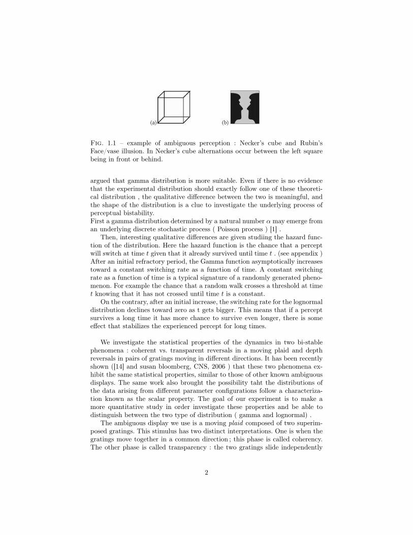
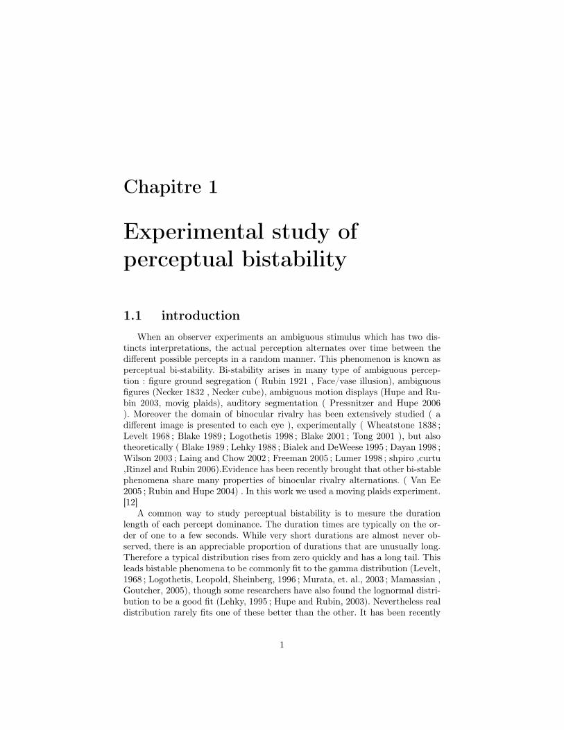
Fig. 1.1 – example of ambiguous perception : Necker’s cube and Rubin’sFace/vase illusion. In Necker’s cube alternations occur between the left squarebeing in front or behind.

argued that gamma distribution is more suitable. Even if there is no evidencethat the experimental distribution should exactly follow one of these theoreti-cal distribution , the qualitative difference between the two is meaningful, andthe shape of the distribution is a clue to investigate the underlying process ofperceptual bistability.First a gamma distribution determined by a natural number α may emerge froman underlying discrete stochastic process ( Poisson process ) [1] .

Then, interesting qualitative differences are given studiing the hazard func-tion of the distribution. Here the hazard function is the chance that a perceptwill switch at time t given that it already survived until time t . (see appendix )After an initial refractory period, the Gamma function asymptotically increasestoward a constant switching rate as a function of time. A constant switchingrate as a function of time is a typical signature of a randomly generated pheno-menon. For example the chance that a random walk crosses a threshold at timet knowing that it has not crossed until time t is a constant.

On the contrary, after an initial increase, the switching rate for the lognormaldistribution declines toward zero as t gets bigger. This means that if a perceptsurvives a long time it has more chance to survive even longer, there is someeffect that stabilizes the experienced percept for long times.

We investigate the statistical properties of the dynamics in two bi-stablephenomena : coherent vs. transparent reversals in a moving plaid and depthreversals in pairs of gratings moving in different directions. It has been recentlyshown ([14] and susan bloomberg, CNS, 2006 ) that these two phenomena ex-hibit the same statistical properties, similar to those of other known ambiguousdisplays. The same work also brought the possibility taht the distributions ofthe data arising from different parameter configurations follow a characteriza-tion known as the scalar property. The goal of our experiment is to make amore quantitative study in order investigate these properties and be able todistinguish between the two type of distribution ( gamma and lognormal) .

The ambiguous display we use is a moving plaid composed of two superim-posed gratings. This stimulus has two distinct interpretations. One is when thegratings move together in a common direction ; this phase is called coherency.The other phase is called transparency : the two gratings slide independently

2

of each other in opposite directions. Over a period of time, the two perceptionsalternate dominance, an example of perceptual bistability. ( see figure 1.2)

Fig. 1.2 – picture of the moving plaid composed of two superimposed gratings.The first interpretation is the coherency interpretation : both gratings are mo-ving in the same direction in a coherent motion. The second interpretation is thetransparency interpretation : the two gratings slide in opposite directions. Another ambiguity in this last interpretation is the relative depth of the gratings.

In the transparency phase of a plaid, there is a further ambiguity regardingthe relative depth of the gratings, or which grating is moving behind the other.There exist conditions in which the transparency phase dominates, such as alarge angle between the gratings (Moreno-Bote, et. al., 2006). We then use thedepth reversals of the transparent plaid as a second ambiguous display to study.

1.2 methodsThis experiment follows very exhaustive qualitative studies of perceptual

bistability based on moving plaids. Our goal is to collect enough duration timesto be able to distinguish between a gamma or a lognormal like distribution.Numerical tests have shown that around 2000 thousand points were enough tomake that distinction. A typical trial lasts 5 minutes and shows around 100 al-ternations. In order to reach that number of points, we set up experiments withlonger sessions, and assuming these distributions follow the scalar property, wecollapse the datas collected on differents sessions for one subject. Moreover ithas been shown recently that the alternation rate had a maximum value for acertain value of the angle between the two gratings [2]. This angle differs fromone subject to the other. This angle was determined for each subject and thenused in the stimulus presented, in order to observe the maximum of alternations.

Each session is constituted of four successive trials of 5 minutes each, whichmakes a twenty minutes long experiment. We found that it was long enough tocalculate mean duration time with a good precision. ( error ≈ 5 percent ) Thefour trial divisions allows the subject to rest for a few minutes before continuingthe experiment. Alternations are reported by the subject by tiping two keys ona computer keyboard. Every reactions are recorded and then analysed in order

3

to eliminate what seem to be error or hesitations of the subject from the datas.For example very short alternation time, which are not likely to really occur,may be caused by hesitations, and are removed from the datas.

For each session, the mean duration time and the standard deviation is com-puted. We compute also the standard error on the mean. Collecting datas onlong sessions allows us to increase the number of time duration we use in calcu-lating the mean, which reduces the standard error on the mean. Then we checkthe scalar property. If it is verified then we can try to collapse the datas collectedon different sessions.

Distributions and hazard functions are computed on matlab. We use anadaptative bining to compute the histograms. Around the mean, where we havelots of points, we distribute bins linearly. In the tail, where we have less points,we distribute the bins exponentially. The bins far in the tail are larger and cancollect more of the few points that remain far from the mean. This allows us tohave less but more accurate points in the tail. We use the original fitting func-tions of matlab to compare experimental distribution and gamma/lognormaldistributions that fit the datas.

1.3 ResultsSessions of 20 minutes gave typically a number of 400 alternations, which

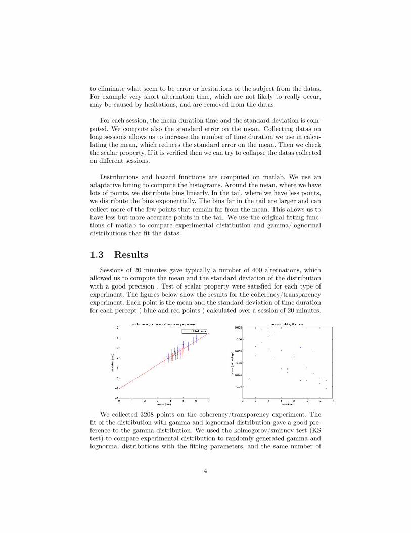
allowed us to compute the mean and the standard deviation of the distributionwith a good precision . Test of scalar property were satisfied for each type ofexperiment. The figures below show the results for the coherency/transparencyexperiment. Each point is the mean and the standard deviation of time durationfor each percept ( blue and red points ) calculated over a session of 20 minutes.

We collected 3208 points on the coherency/transparency experiment. Thefit of the distribution with gamma and lognormal distribution gave a good pre-ference to the gamma distribution. We used the kolmogorov/smirnov test (KStest) to compare experimental distribution to randomly generated gamma andlognormal distributions with the fitting parameters, and the same number of

4

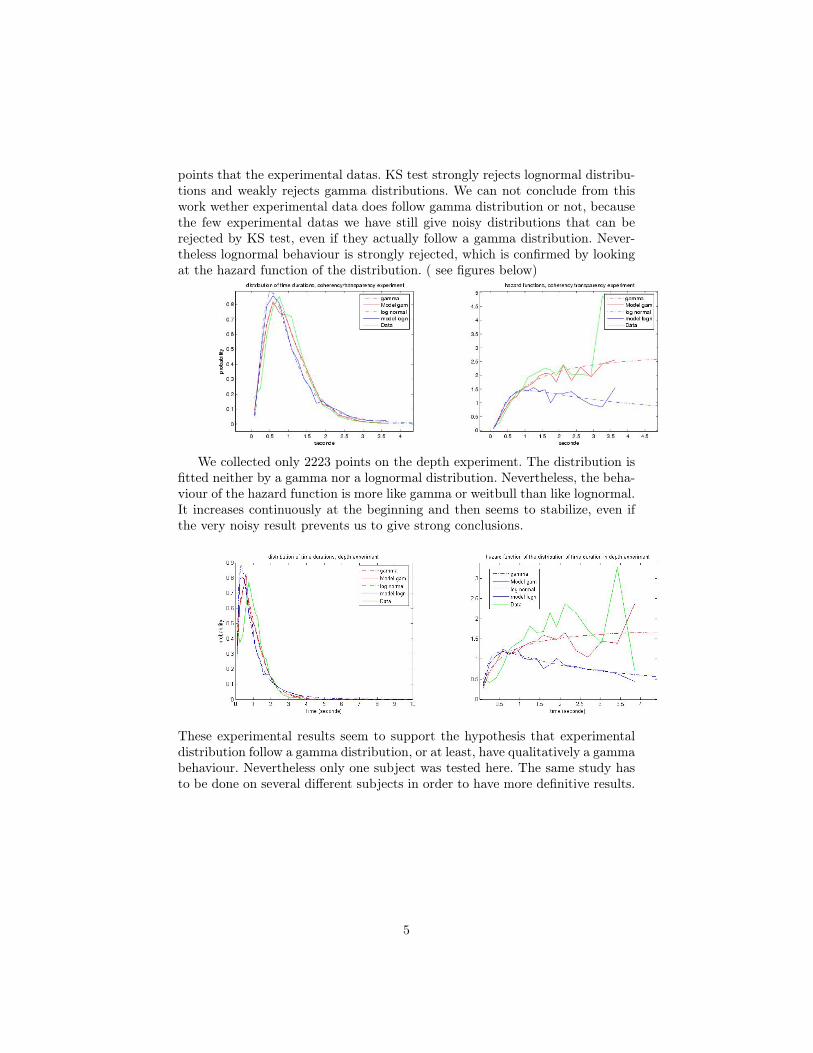
points that the experimental datas. KS test strongly rejects lognormal distribu-tions and weakly rejects gamma distributions. We can not conclude from thiswork wether experimental data does follow gamma distribution or not, becausethe few experimental datas we have still give noisy distributions that can berejected by KS test, even if they actually follow a gamma distribution. Never-theless lognormal behaviour is strongly rejected, which is confirmed by lookingat the hazard function of the distribution. ( see figures below)

We collected only 2223 points on the depth experiment. The distribution isfitted neither by a gamma nor a lognormal distribution. Nevertheless, the beha-viour of the hazard function is more like gamma or weitbull than like lognormal.It increases continuously at the beginning and then seems to stabilize, even ifthe very noisy result prevents us to give strong conclusions.

These experimental results seem to support the hypothesis that experimentaldistribution follow a gamma distribution, or at least, have qualitatively a gammabehaviour. Nevertheless only one subject was tested here. The same study hasto be done on several different subjects in order to have more definitive results.

5

Chapitre 2

Dynamics of perceptualbistability

2.1 introduction and starting point : an attractormodel for perceptual bistability

As said before, perceptual bistability has been widely studied theoriticaly.The general way to modelize this phenomenon is to use two distinct popula-tions of neuron competing for their own activity. The activity of one populationwhile the other is inactive is interpreted as the perception of one of the twointerpretations. Activity of both population at the same time is interpretated asfusion ( percepted image is a complex combination of the two interpretations).The dominant view is that alternations arise from some form of slow adaptationacting on the dominant population, either in its firing rate or in its synapticoutput ( synaptic depression )or both, that leads to a switch in dominance tothe competing population (Lehky 1988 ; Wilson 2003 ;Laing and Chow 2002 ;Matsuoka 1984 ; Stollenwerk and Bode 2003 ; Lago-Fernandez and Deco 2002 ;Kalarickal and Marshall 2000). These models are deterministic and generatealternations with a perfect periodicity. Noise can still be introduced in the mo-del to fit better the experiments. In the equations, adaptation generally takesthe form of a negative feedback to the firing rate or synaptic output. In thisview, only one state of activity of the neural network is stable at one time. Thisstate is progressively weakened as adaptation arises until it is the other state ofactivity that becomes stable. Typical tragectories in the activity plane can beviewed in the appendix .

It has been recently proposed [3] that noise can be the primary cause foralternations. Noise exists in the brain at multiple scales, from vesicular releaseand spiking variability to fluctuations in global neurotransmitter levels. Also,external noise can cause perceptual alternations ( blinking, uncontrolled mo-vements of the head ) . In this scheme, each of the competing percepts can

6

be viewed as a stable state of the neuronal dynamics, with noise causing thesystem to alternate between them. The so-called noise-driven attractor modelspredict that perceptual alternations would cease if noise is removed from thesystem : the system would settle down in one of the two percepts and stay thereindefinitely.

Two important experimental observations have been made in the field ofbinocular rivalry, where the strength of each competing percept can be manipu-lated independently. Levelt’s (1968) proposition II states that weakening onlyone image while keeping the other fixed increases the dominance duration ofthe unchanged image, with little effect on the dominance duration of the mani-pulated one. Levelt’s proposition IV states that when the monocularimages arestrengthened simultaneously, the mean durations of both eyes decrease [4].

The model studied here is the noise-driven attractor model proposed in [3] . Itis consistent with levelt’s proposition II and IV. Since the dynamics of attractornetworks can be easily interpreted using an energy model, the first step is to findan energy-based formalism consistent with the observations summarized above.The two attractors can be seen as the two local stable state of a double wellenergy function. The bigger the energy barrier between one stable state and theother is, the more stable is the attractor.

Levelt’s proposition II implies that an increase of the input to population Ahas the effect to heightening the energy barrier of the population representingpercept B : it is more difficult to produce noisy tragectories that escape fromattractor B. Levelt’s proposition IV implies that increasing both inputs lowersthe energy barrier. A simple energy function that has these two properties is :

E(∆r) = ∆r2(∆r2 − 2) + gA(∆r − 1)2 + gB(∆r + 1)2

Here ∆r = rA − rB is the difference between the firing rate of the twopopulations. gA and gB are their input strength. This energy function has tominima, located close to ∆r = ±1, which respectively correspond to dominantactivity of population A, and to dominant activity of population B. ( here firingrates are dimensionless, maximum activity is equal to one ). The quadratic termsproportionnal to gA and gB influence the depth of the minima. Each increasesthe energy of the competing minimum without changing its own energy.

2.2 modelsA rate-based network model can be built on the energy description of levelt II

and IV. First the one-variable energy function can be extended to a two-variableenergy function, where the two variables stand for the firing rates rA and rB

of the two populations. Two coupled differential equations can be derived fromthis energy. They describe the dynamics of the two populations’ firing rates.(see appendix)

7

τd

dtrA = −rA + f(αrA − βrB + gA − (gA + gB)rA + aA + nA)

τd

dtrB = −rB + f(αrB − βrA + gB − (gA + gB)rB + aB + nB)

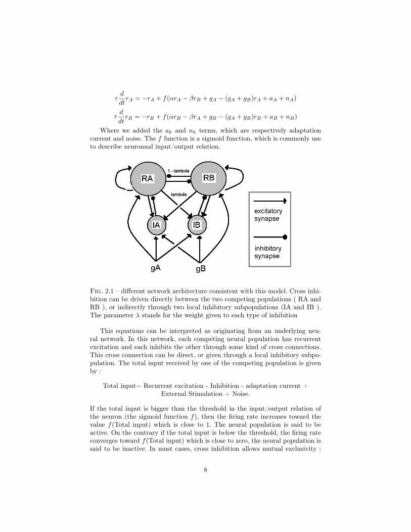
Where we added the ak and nk terms, which are respectively adaptationcurrent and noise. The f function is a sigmoid function, which is commonly useto describe neuronnal input/output relation.

Fig. 2.1 – different network architecture consistent with this model. Cross inhi-bition can be driven directly between the two competing populations ( RA andRB ), or indirectly through two local inhibitory subpopulations (IA and IB ).The parameter λ stands for the weight given to each type of inhibition

This equations can be interpreted as originating from an underlying neu-ral network. In this network, each competing neural population has recurrentexcitation and each inhibits the other through some kind of cross connections.This cross connection can be direct, or given through a local inhibitory subpo-pulation. The total input received by one of the competing population is givenby :

Total input= Recurrent excitation - Inhibition - adaptation current +External Stimulation + Noise.

If the total input is bigger than the threshold in the input/output relation ofthe neuron (the sigmoid function f), then the firing rate increases toward thevalue f(Total input) which is close to 1. The neural population is said to beactive. On the contrary if the total input is below the threshold, the firing rateconverges toward f(Total input) which is close to zero, the neural population issaid to be inactive. In must cases, cross inhibition allows mutual exclusivity :

8

when population A is active, population B receives a strong negative input.Then total input received by population B is below the threshold and it staysinactive. Both alternations and winner-take-all behaviour are compatible withmutual exclusivity.

An novel feature of the model is that the firing rates of the local inhibitorysubpopulations depends on the total external stimulation. Each competing po-pulation k receives back inhibition equaling (gA +gB)rk . This feature is a directconsequence of the multiplicative term gk(∆r ± 1) in the one variable energyfunction, which itself is required to make the model behave in accordance withLevelt’s proposition II and IV. An other particular feature of this model is thestrong recurrent excitatory connection, which produces robust winner-take-allbehaviour in the absence of noise. Then, we expect oscillation to be mainly noiseinduced.

In our case, we do not want adaptation to be strong enough to produce al-ternations on its own. Alternations are due to noise that occasionally producestrajectory that cross the threshold between the two stable states : the totalinput to dominant population goes weaker whereas the total input to inactivepopulation suddenly becomes bigger than the threshold, giving rise to a switchin dominance. In other words, noise allows the system to cross the energy barrierbetween its two stable states. Nevertheless, adaptation can still have a role toplay. As the adaptation current increases over time, the probability increasesthat a fluctuation due to noise will cause the total input to dip below the thre-shold. Still, if the strength of adaptation is small, alternations are not driven bya gradual decrease of the total input below a threshold ( as in oscillator modelsof bistability) but rather by chance, when noise-induced fluctuations bring thetotal input below the threshold. Adaptation is added to this model even if itdoes not play the main role. Adaptation mechanisms are very common in thebrain, and here it helps to produce distributions of time durations which res-semble the skewed gaussian observed experimentally.

Different network architectures can be used to study this model. In the firstone, cross inhibition is driven directly between the two competing population.We call this model DCI for Direct Cross Inhibition. In the second one, ( figure2.1 ) cross inhibition is driven indirectly through the local inhibitory subpopu-lations. We call this model ICI for Indirect Cross Inhibition. This difference isimportant because in the DCI model, cross inhibition is linearly added to thetotal input of a competing population. In the ICI model, cross inhibition goesthrough the input/output relation of the local inhibitory sub-population. So theway cross inhibition is felt by the competing populations is not the same in bothcases.

We know that we must choose the input/output relation of the local inhi-bitory subpopulation so that the competing population receives back inhibitionequaling (gA + gB)rk. A simple way to do so is to choose a multiplicative in-put/output relation of the form :

– (gA + gB)rA in the DCI model. ( cross inhibition does not pass through

9

local inhibitory population)– (gA + gB)(rA + rB) in the ICI model. ( cross inhibition is entirely driven

by local inhibitory population)An other way is to a quadratic input/output relation of the form :– (gA + gB + ηrA)2 in the DCI model.– (gA + gB + ηrA + φrB)2 in the ICI model.The parameter η and φ are chosen in order to give the good back inhibition

term to the competing population. Both DCI with multiplicative relation andICI with quadratic relation were studied in [3] . It has been shown that bothmodels could be mapped into each other for particular sets of parameters. Wekept the parameter set chosen in [3], which give dynamics consistent with Le-velt’s proposition.

First, the DCI architecture with a quadratic gating and ICI architecture witha multiplicative gating were studied. Then„we introduced a weighting factor λin the equations. When λ = 1 , direct cross inhibition is full weighted, andno input goes from a competing population to the opposite local inhibitorysubpopulation. When λ = 0, no weight is given to direct cross inhibition andmutual exclusivity is provided exclusively by local inhibititory subpopulation.Changing continuously the value of λ allowed us to move continously from theDCI architecture to the ICI architecture, which opens a new range of possiblemodels. Our interest here is to know what kind of model satisfy the most levelt’sproposition II and IV.

2.3 resultsthe parameters chosen for this study are : α = 0.75, β = 0.8 , βi = 0.5

, γ = 0.1 , σ (noise amplitude) = 0.06 . This choice of parameter is justifiedin the appendix. The phase plane and figures below were obtained using a csimulation. Models were also studied with xpp and auto.

2.3.1 study of the model with a quadratic gating

10

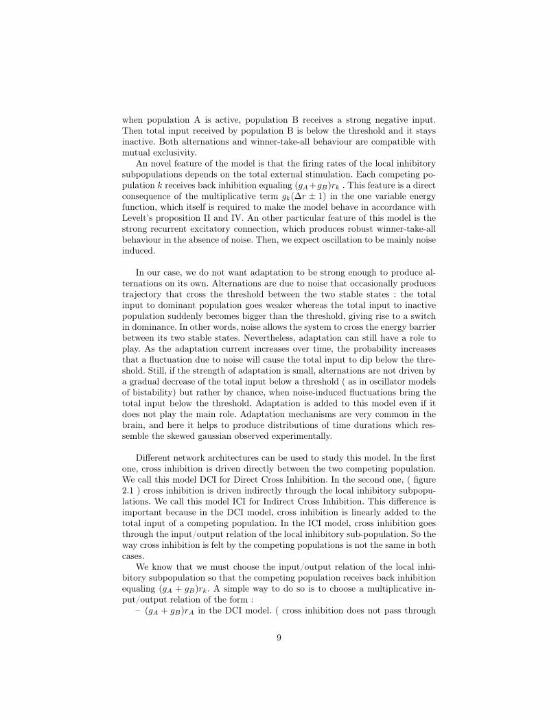
The left figure is the bifurcation diagram for λ = 0 ( ICI architecture ),the right figure is the bifurcation diagram for λ = 1. The diagram shows themaximum and minimum activity of each population. Both are very similar.For very low input, population are inactive. For high input ,there is fusion :both populations are equally active, there are no alternations (the differencemaximum/minimum observed here is only due to noise ). In the between, activityalternates between the two population (oscillatory regime, OSC). Here noise isstrong enough to generate alternations everywhere, but for weaker noise, onewould see a Winner Take All (WTA) region between the oscillatory regime andthe no activity regime. The two models are very similar. Intermediate values ofλ did not show any significative changes.

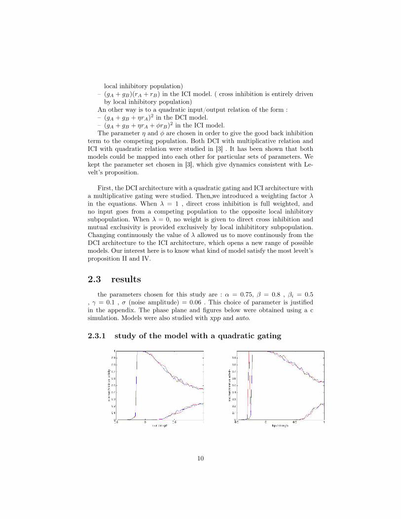
The upper figures show the evolution of the mean dominance time as inputstrength increases. For ICI model ( λ = 0), Levelt IV is well verified. there isa very narrow increase of < T > at the beginning, but < T > mainly followsa decreasing trajectory. This result is just a confirmation of what has alreadybeen observed in (reference). On the other hand, the DCI model with a quadraticgating does not give a behaviour consistent with levelt IV. < T > follows a longincreasing tragectories for intermediate input, and then decreases for higherinput strength. Intermediate values of λ show this increasing part of < T >widening continuously.

The lower figures show the evolution of the mean dominance of each perceptwhen the input given to one of them is increased while the other is kept fixed.The mean dominance time of the population whose input strength is increasingdecreases, while the other increases. This result is consistent with what has beenfound previously in [3] , even it is not exactly what states Levelt’s propositionII, it the same kind of behaviour.

11

2.3.2 study of the model with a multiplicative gating

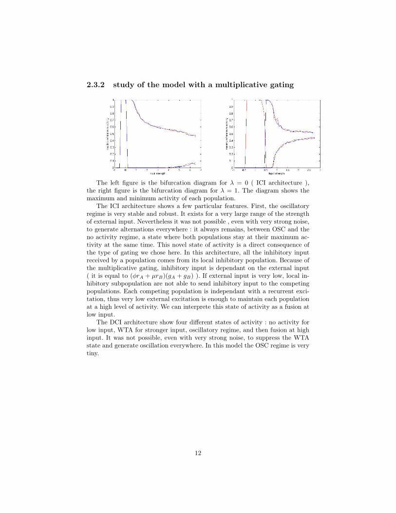
The left figure is the bifurcation diagram for λ = 0 ( ICI architecture ),the right figure is the bifurcation diagram for λ = 1. The diagram shows themaximum and minimum activity of each population.

The ICI architecture shows a few particular features. First, the oscillatoryregime is very stable and robust. It exists for a very large range of the strengthof external input. Nevertheless it was not possible , even with very strong noise,to generate alternations everywhere : it always remains, between OSC and theno activity regime, a state where both populations stay at their maximum ac-tivity at the same time. This novel state of activity is a direct consequence ofthe type of gating we chose here. In this architecture, all the inhibitory inputreceived by a population comes from its local inhibitory population. Because ofthe multiplicative gating, inhibitory input is dependant on the external input( it is equal to (φrA + µrB)(gA + gB) ). If external input is very low, local in-hibitory subpopulation are not able to send inhibitory input to the competingpopulations. Each competing population is independant with a recurrent exci-tation, thus very low external excitation is enough to maintain each populationat a high level of activity. We can interprete this state of activity as a fusion atlow input.

The DCI architecture show four different states of activity : no activity forlow input, WTA for stronger input, oscillatory regime, and then fusion at highinput. It was not possible, even with very strong noise, to suppress the WTAstate and generate oscillation everywhere. In this model the OSC regime is verytiny.

12

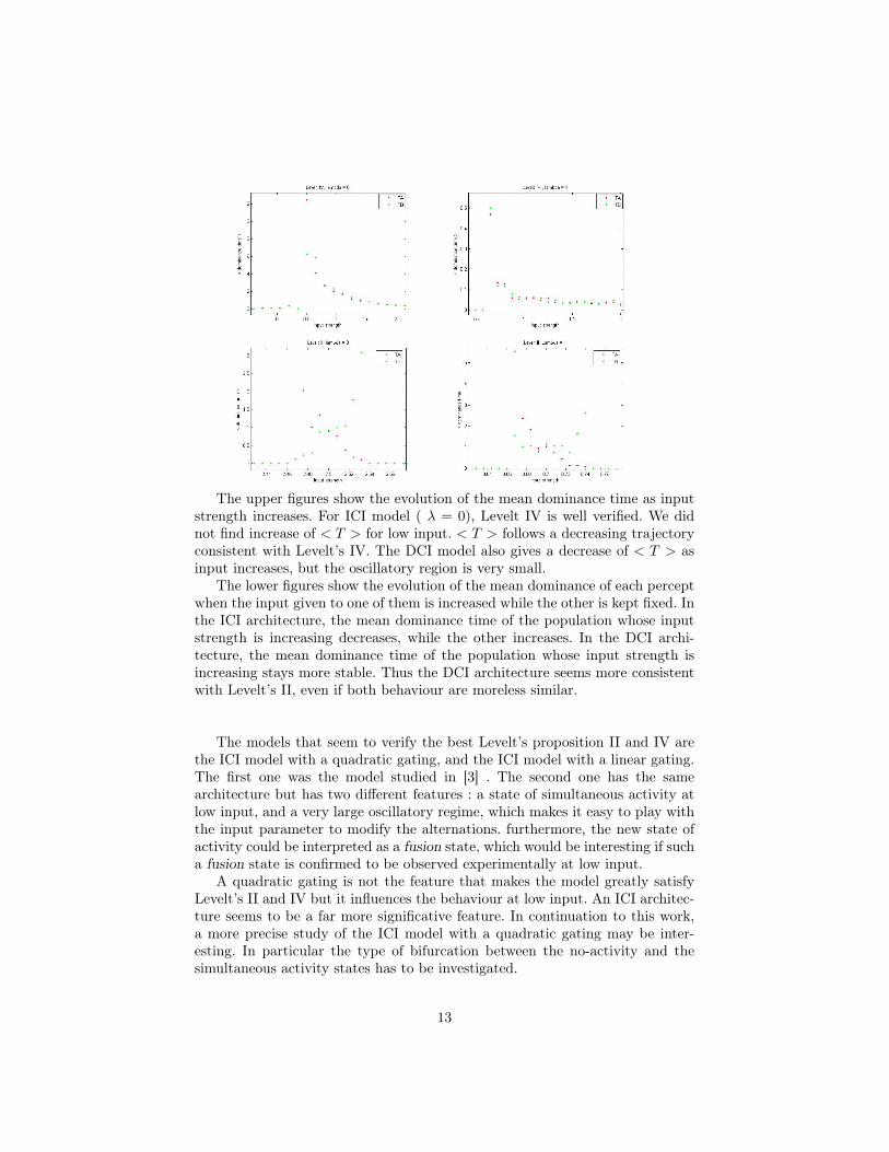
The upper figures show the evolution of the mean dominance time as inputstrength increases. For ICI model ( λ = 0), Levelt IV is well verified. We didnot find increase of < T > for low input. < T > follows a decreasing trajectoryconsistent with Levelt’s IV. The DCI model also gives a decrease of < T > asinput increases, but the oscillatory region is very small.

The lower figures show the evolution of the mean dominance of each perceptwhen the input given to one of them is increased while the other is kept fixed. Inthe ICI architecture, the mean dominance time of the population whose inputstrength is increasing decreases, while the other increases. In the DCI archi-tecture, the mean dominance time of the population whose input strength isincreasing stays more stable. Thus the DCI architecture seems more consistentwith Levelt’s II, even if both behaviour are moreless similar.

The models that seem to verify the best Levelt’s proposition II and IV arethe ICI model with a quadratic gating, and the ICI model with a linear gating.The first one was the model studied in [3] . The second one has the samearchitecture but has two different features : a state of simultaneous activity atlow input, and a very large oscillatory regime, which makes it easy to play withthe input parameter to modify the alternations. furthermore, the new state ofactivity could be interpreted as a fusion state, which would be interesting if sucha fusion state is confirmed to be observed experimentally at low input.

A quadratic gating is not the feature that makes the model greatly satisfyLevelt’s II and IV but it influences the behaviour at low input. An ICI architec-ture seems to be a far more significative feature. In continuation to this work,a more precise study of the ICI model with a quadratic gating may be inter-esting. In particular the type of bifurcation between the no-activity and thesimultaneous activity states has to be investigated.

13

Chapitre 3

two models for persistance

3.1 principles and ideasThe previous sections, both experimental and theoretical, dealt with conti-

nuous stimulation presented to the subject, or the the neural network. The mainaspect of the response of the studied system ( both real and theoretical ) to thestimulus, is to weaken the first experienced percept and to increase the chanceto switch to the other one. This behavior corresponds to the initial increaseof the hazard function of the experimental distribution, and to the adaptationused in nearly all neural networks to produce ( adaptation-driven alternations)or facilitate (noise-driven alternations) alternations. however, an other type oftime dependant response of the system to stimulations has been brought in lightexperimentally. Intermittent stimulation ( ie periodic short presentations of thestimulus separated by blank period ) seem to produce some stabilizing effect onthe system generating the alternations. Perceptual alternations can be slowed,and even avoided, in the case of intermittent stimulus ( [5], joshua braun 2007) . This phenomenon can be called as persistance. It has, on apparently longertime scales, the opposite effect of the adaptation discussed above.

Here we propose two models that predict some form of persistance, and areconsistent with some experimental facts. Our starting point is the ICI modelwith a quadratic relation studied above. We modify this model in two differentway in order to get persistance.

As seen previously, the studied model has two distinct stable attractors thatcan be weakened under the effect of adaptation. An alternation occurs whennoise produces a tragectory that escapes the attraction region of an attractorand goes into the attraction region of the second one, and then converges towardthis second attractor. These two regions of attraction are separated in the acti-vity phase plane by a frontier called separatrix. ( see figure 3.1 )The evolution ofthe separatrix over time plays a major role in the understanding of persistanceeffect, in particular in the case of intermittent stimulation.

14

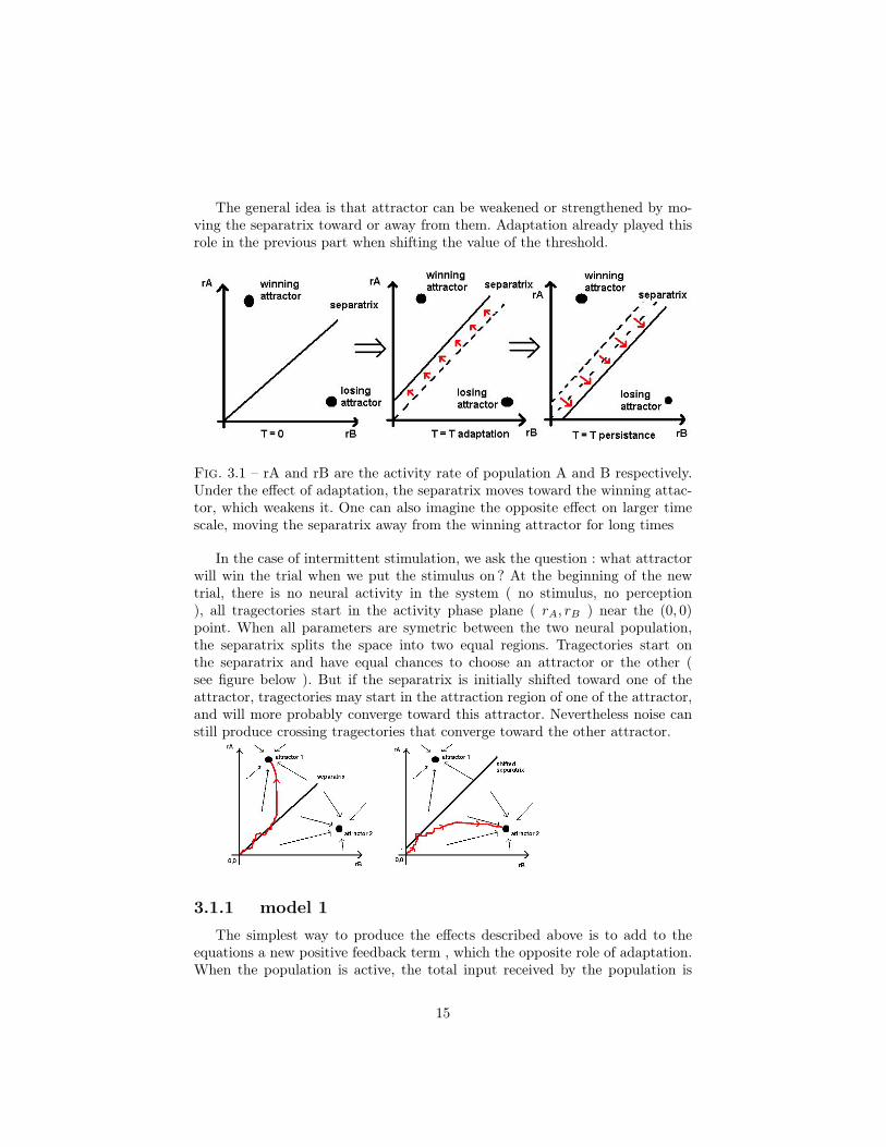
The general idea is that attractor can be weakened or strengthened by mo-ving the separatrix toward or away from them. Adaptation already played thisrole in the previous part when shifting the value of the threshold.

Fig. 3.1 – rA and rB are the activity rate of population A and B respectively.Under the effect of adaptation, the separatrix moves toward the winning attac-tor, which weakens it. One can also imagine the opposite effect on larger timescale, moving the separatrix away from the winning attractor for long times

In the case of intermittent stimulation, we ask the question : what attractorwill win the trial when we put the stimulus on ? At the beginning of the newtrial, there is no neural activity in the system ( no stimulus, no perception), all tragectories start in the activity phase plane ( rA, rB ) near the (0, 0)point. When all parameters are symetric between the two neural population,the separatrix splits the space into two equal regions. Tragectories start onthe separatrix and have equal chances to choose an attractor or the other (see figure below ). But if the separatrix is initially shifted toward one of theattractor, tragectories may start in the attraction region of one of the attractor,and will more probably converge toward this attractor. Nevertheless noise canstill produce crossing tragectories that converge toward the other attractor.

3.1.1 model 1The simplest way to produce the effects described above is to add to the

equations a new positive feedback term , which the opposite role of adaptation.When the population is active, the total input received by the population is

15

slowly increased by an additional current, ( pA term in the equations ). thispersistance term tends exponentialy to a positive value when the correspondingpopulation is active. The corresponding time scale is taken to be longer ( ≈ 20sec ) than the timescale of adaptation ( ≈ 2 sec ).

This simple method has been used in [6] in order to find persistance effect ina deterministic model ( adaptation-driven alternations ). In their model adap-tation terms and persistance terms have the same time scale but they have adifferent action on the separatrix : the adaptation is activity dependant and donot shift the separatrix near the the (0, 0) point.

We can justify the use of the pA term saying that it seems to be the lo-west order and simplest way to break the symmetry in an activity dependantway. But it is hard to have real neurophysiological interpretations of this term.It could still be interpreted as a mean-field term emerging from an underlyingmore complex structure.

We study this model the case where alternations are driven by adaptation, and in the case where they are noise-driven. Even in the case of noise-drivenalternations, adaptation plays a role in increasing the probability to switch whileadaptation increases. The importance of noise in our choice of parameter makeboth cases no deterministic.

equations :

˙rA = (−rA + f(αrA − βirAi− aA + pA + nA))/τ

˙rB = (−rB + f(αrB − βirBi− aB + pB + nB))/τ

˙aA = (−aA + γarA)/τa

˙aB = (−aB + γarB)/τa

˙pA = (−pA + γprA)/τp

˙pB = (−pB + γprB)/τp

For short time scale, adaptation moves the separatrix toward the winningattractor. If the population remains active for a long time, the separatrix movesback to its initial value under the persistance term effect, making it more diffi-cult for the noise to produce crossing tragectories, and so stabilizing the winningattractor in the long run. This effect can be conserved in the case of intermit-tent stimulation because the adaptation and persistance term are not activitydependant and keep their effect through the no-stimulus periods. Negative feed-back (adaptation), with a shorter time scale, relaxes faster than the positivefeedback. This results in a shift of the separatrix between the attractors. Whentrajectories start at the no-activity point ( when we put stimulus back ) , if theseparatrix is shifted toward the attractor that has losed the previous stimula-tion, it increases the probability that the tragectory chooses the attractor whichhas won previously.

16

3.1.2 model 2The other scheme consists in modifying the synaptic parameters in the mo-

del. Here we put neither adapation ( negative feedback ) nor positive feedback.Alternations are purely noise driven.

We assume that the coefficient of recurrent excitation α can evolve over time.This evolution is interpretated as a modification of the ability of the synapse ofthe recurrent connection to transmit the signal. If this ability is strengthen ( ieα is bigger ), then it makes the corresponding population more likely active (the population can more easily support its own activity ) .

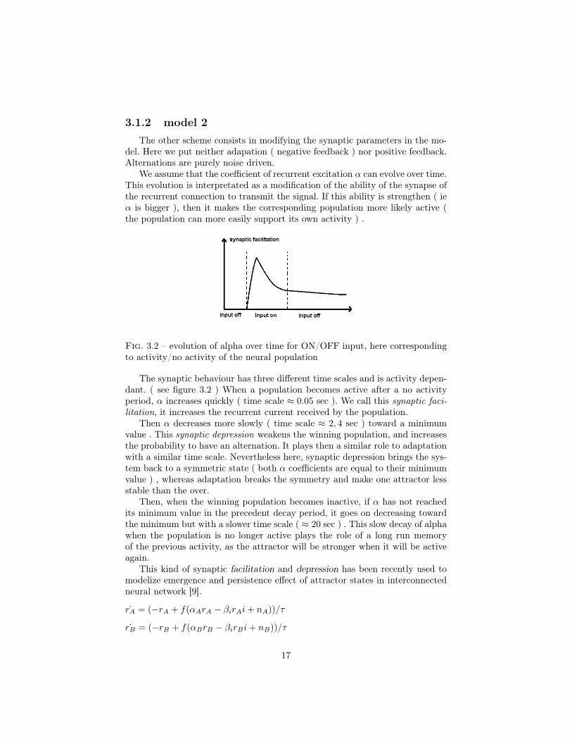
Fig. 3.2 – evolution of alpha over time for ON/OFF input, here correspondingto activity/no activity of the neural population

The synaptic behaviour has three different time scales and is activity depen-dant. ( see figure 3.2 ) When a population becomes active after a no activityperiod, α increases quickly ( time scale ≈ 0.05 sec ). We call this synaptic faci-litation, it increases the recurrent current received by the population.

Then α decreases more slowly ( time scale ≈ 2, 4 sec ) toward a minimumvalue . This synaptic depression weakens the winning population, and increasesthe probability to have an alternation. It plays then a similar role to adaptationwith a similar time scale. Nevertheless here, synaptic depression brings the sys-tem back to a symmetric state ( both α coefficients are equal to their minimumvalue ) , whereas adaptation breaks the symmetry and make one attractor lessstable than the over.

Then, when the winning population becomes inactive, if α has not reachedits minimum value in the precedent decay period, it goes on decreasing towardthe minimum but with a slower time scale ( ≈ 20 sec ) . This slow decay of alphawhen the population is no longer active plays the role of a long run memoryof the previous activity, as the attractor will be stronger when it will be activeagain.

This kind of synaptic facilitation and depression has been recently used tomodelize emergence and persistence effect of attractor states in interconnectedneural network [9].

˙rA = (−rA + f(αArA − βirAi + nA))/τ

˙rB = (−rB + f(αBrB − βirBi + nB))/τ

17

αA = α(1 + δA)

δA = δAIN + δAoff

The exact equations of δ evolution are given in the annexe.

3.2 Results

3.2.1 distribution of time dominanceWe run the three models in the case of a continuous stimulation in order to

have up to 50 000 alternations. We then computed the distribution and hazardfunction in the same way we did in the experimental part.

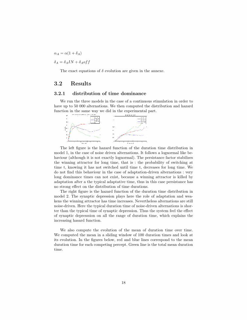
The left figure is the hazard function of the duration time distribution inmodel 1, in the case of noise driven alternations. It follows a lognormal like be-haviour (although it is not exactly lognormal). The persistance factor stabilizesthe winning attractor for long time, that is : the probability of switching attime t, knowing it has not switched until time t, decreases for long time. Wedo not find this behaviour in the case of adaptation-driven alternations : verylong dominance times can not exist, because a winning attractor is killed byadaptation after a the typical adaptative time, thus in this case persistance hasno strong effect on the distribution of time durations.

The right figure is the hazard function of the duration time distribution inmodel 2. The synaptic depression plays here the role of adaptation and wea-kens the winning attractor has time increases. Nevertheless alternations are stillnoise-driven. Here the typical duration time of noise-driven alternations is shor-ter than the typical time of synaptic depression. Thus the system feel the effectof synaptic depresssion on all the range of duration time, which explains theincreasing hasard function.

We also compute the evolution of the mean of duration time over time.We computed the mean in a sliding window of 100 duration times and look atits evolution. In the figures below, red and blue lines correspond to the meanduration time for each competing percept. Green line is the total mean durationtime.

18

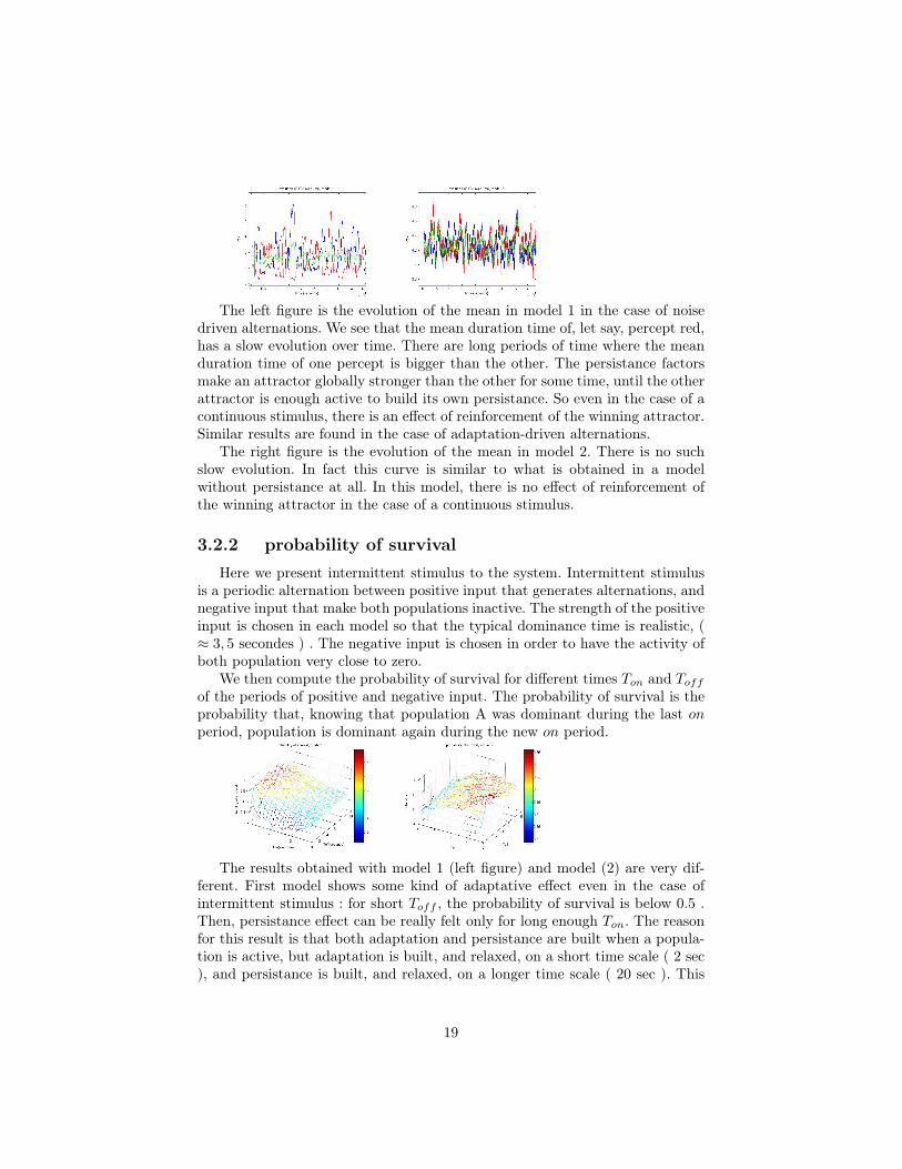
The left figure is the evolution of the mean in model 1 in the case of noisedriven alternations. We see that the mean duration time of, let say, percept red,has a slow evolution over time. There are long periods of time where the meanduration time of one percept is bigger than the other. The persistance factorsmake an attractor globally stronger than the other for some time, until the otherattractor is enough active to build its own persistance. So even in the case of acontinuous stimulus, there is an effect of reinforcement of the winning attractor.Similar results are found in the case of adaptation-driven alternations.

The right figure is the evolution of the mean in model 2. There is no suchslow evolution. In fact this curve is similar to what is obtained in a modelwithout persistance at all. In this model, there is no effect of reinforcement ofthe winning attractor in the case of a continuous stimulus.

3.2.2 probability of survivalHere we present intermittent stimulus to the system. Intermittent stimulus

is a periodic alternation between positive input that generates alternations, andnegative input that make both populations inactive. The strength of the positiveinput is chosen in each model so that the typical dominance time is realistic, (≈ 3, 5 secondes ) . The negative input is chosen in order to have the activity ofboth population very close to zero.

We then compute the probability of survival for different times Ton and Toff

of the periods of positive and negative input. The probability of survival is theprobability that, knowing that population A was dominant during the last onperiod, population is dominant again during the new on period.

The results obtained with model 1 (left figure) and model (2) are very dif-ferent. First model shows some kind of adaptative effect even in the case ofintermittent stimulus : for short Toff , the probability of survival is below 0.5 .Then, persistance effect can be really felt only for long enough Ton. The reasonfor this result is that both adaptation and persistance are built when a popula-tion is active, but adaptation is built, and relaxed, on a short time scale ( 2 sec), and persistance is built, and relaxed, on a longer time scale ( 20 sec ). This

19

explains why adaptative effects are felt for short Ton and Toff , and persistanceeffects felt for long Ton and Toff .

The dynamics of model 2 is very different. A winning attractor is reinforcedon a very short time scale (synaptic facilitation). But if the population remainsactive for too long, the reinforcement disappears slowly (synaptic depression).The resulting bias at the end of a Ton period relaxes very slowly. This explainswhy in this model persistance is felt for short Ton. Also there is no adaptativeeffect in this model (probability is always above 0.5 ) .

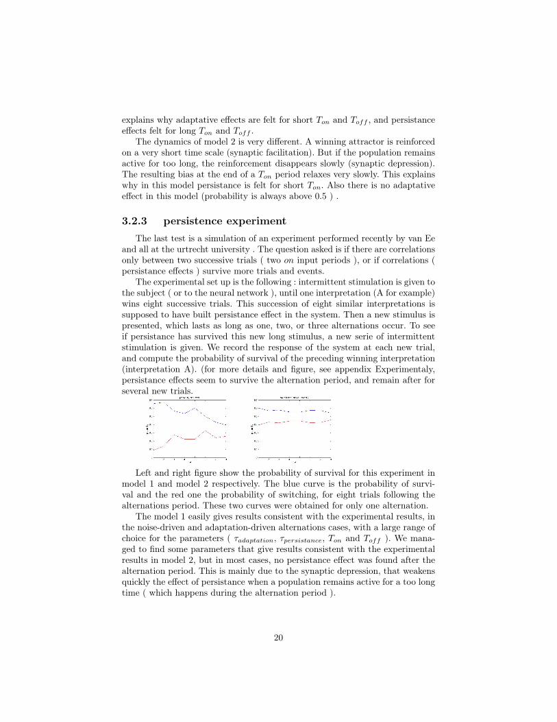
3.2.3 persistence experimentThe last test is a simulation of an experiment performed recently by van Ee

and all at the urtrecht university . The question asked is if there are correlationsonly between two successive trials ( two on input periods ), or if correlations (persistance effects ) survive more trials and events.

The experimental set up is the following : intermittent stimulation is given tothe subject ( or to the neural network ), until one interpretation (A for example)wins eight successive trials. This succession of eight similar interpretations issupposed to have built persistance effect in the system. Then a new stimulus ispresented, which lasts as long as one, two, or three alternations occur. To seeif persistance has survived this new long stimulus, a new serie of intermittentstimulation is given. We record the response of the system at each new trial,and compute the probability of survival of the preceding winning interpretation(interpretation A). (for more details and figure, see appendix Experimentaly,persistance effects seem to survive the alternation period, and remain after forseveral new trials.

Left and right figure show the probability of survival for this experiment inmodel 1 and model 2 respectively. The blue curve is the probability of survi-val and the red one the probability of switching, for eight trials following thealternations period. These two curves were obtained for only one alternation.

The model 1 easily gives results consistent with the experimental results, inthe noise-driven and adaptation-driven alternations cases, with a large range ofchoice for the parameters ( τadaptation, τpersistance, Ton and Toff ). We mana-ged to find some parameters that give results consistent with the experimentalresults in model 2, but in most cases, no persistance effect was found after thealternation period. This is mainly due to the synaptic depression, that weakensquickly the effect of persistance when a population remains active for a too longtime ( which happens during the alternation period ).

20

The two models studied above both predict some kind of persistance effectbut make quite different predictions. First a quantitative study of the durationtime distribution and of its hazard function coud be useful to distinguish betweenthe two : some stabilizing effect of a dominant population in the long time shouldshow a decreasing hazard function. If not, model 1 in the case of adaptation-driven alternations or model 2 are our only good candidates. Since more andmore evidences are made that alternations are noise-driven, the choice of model2 seems to be a better choice. Our experimental results support that last optionbut they are not definitive.

Also, we have seen that model 2 did not show persistance effect in the case ofa continuous stimulation. An experimental study of the evolution of < T > overtime would be interesting to investigate that point, but it should be difficult :differences between the two models can be seen after a stimulus of at least 5000secondes. So long stimulus can not be realistically presented to a living subject.

Finally, the prediction of the probability of survival are different in the twomodels. A comparison with experimental results could give a preference to oneor the other.

ConclusionThree different aspects of the perceptual bistability phenomenum were stu-

died in this work. The experimental study was the occasion to learn the basicconcepts of perceptual bistability, and was a good introduction to the methodsof psychophysics. Even if not complete, our results support the hypothesis thatexperimental distributions follow a gamma-like behaviour.

Several new neural network models of perceptual bistability were studied,based on the noise-induced model of Ruben Moreno Bote. Our study shown thatan ICI (indirect cross inhibition) architecture seems to be an important featurein order to produce results in consistence with Levelt’s propositions II and IV.

Also, two neural network models were built in order to simulize some kindof persistance effects. The two models make quite different predictions whichcould be investigated experimentally.

AcknowledgmentsWe would like to thank Nava Rubin and John Rinzel for directing this work.We thank Asya Shpiro and Ruben Moreno-Bote for their helpful comments anduseful discussions. We also liked to thank Bob shapley and the CNS for theirfinancial support.

21

bibliography[1] Discrete stochastic process underlying peceptual rivalry , Murata, Matsui,

Miyauchi, Kakita, Yanagida , Neuroreport 14 1347[2] Maximum alternation rate in bi-stable perception occurs at equidomi-

nance , Shpiro, Moreno-bote, Bloomber, Rubin and Rinzel, poster, 2007[3] Noise-induced alternations in an attractor network model of perceptual

bi-stability , Moreno-Bote , Rinzel, Rubin, Journal of neurophysiology[4] Levelt WJM. On binocular rivalry. The Hague - Paris : Mouton, 1968 .[5] stable perception of visually ambiguous patterns, david a. leopold, melanie

wilke, alexander maier and nikos k.logothetis. nature neuroscience volume 5 no6, june 2002.

[6] Percept choice sequences driven by interrupted ambiguous stimuli : A low-level neural model Noest, Van Ee, Nijs, Van Wezel. Journal of vision, 7(8) :10,1-14.

[7] Dynamical characteristics common to neuronal competition models shpiro,Curtu, Rinzel, Rubin . Journal pf neurophysiology 97 : 462-473,2007 .

[8] A recurrent network mechanism of time integration in perceptual deci-sions Wong and wang, journal of neuroscience, 26(4) :1314-1328, 2006.

[9] Persistent activity in neural networks with dynamic synapses Barak, Tso-dyks, Plos Comput Biol, 2007 May 25 ; 3(5) ;e104.

[10] Visuel wahrgenommene Figuren. Rubin E. Copenhagen : Gyldendals,1921.[11] Observations on some remarkable phenomenon which occurs on viewing

a figure of a crystal of geometrical solid Lond, Edinburgh Phil. Mag. Jl Sci 3 :329-337, 1832

[12] The dynamics of bi-stable alternations in ambiguous motion displays :a fresh look at plaids. Vision Res 43 :531-548, 2003.

[13] A spiking neuron model for binocular rivalry. Laing and Chow, J computNeuroscience 12 :39-53, 2002.

[14] Dynamics of perceptual bistability : plaids and binocular rivalry com-pared. Rubin and Hupe. In Binocular rivalry, edited by Alais and Blake. Cam-bridge, MA : MIT Press ; 2004.

22

Chapitre 4

appendix

4.0.4 hazard functionLet’s consider a normalized distribution f(t), which gives the probability

that an event occurs at time t. The hazard function of f is the probabilitythat event occurs at t, knowing that it has not occured until time t. This is aconditionnal probability and it is equal to :

H(t) =f(t)

1−∫ t

0f(t)

4.0.5 trajectories in the activity planesee figure 4.1 .

4.0.6 construction of the rate-based networkWe can construct an energy function, based on the single variable energy

function see above, for a network with two populations, A and B, that are firingat rates rA and rB respectively :

E(rA, rB) = −12(αr2

A + αr2B − 2βrArB)

+12gA((1− rA)2 + r2

B) +12gB((1− rB)2 + r2

A) +∑

i

∫ ri

0

f−1(u)du

Here firing rates are dimensionless, so that 0 ≤ rA, rB ≤ 1 . f−1 is theinverse function of a neuronal population’s input-output relation ( firing rate =f(input) ). gA ad gB are the external input given to each population.

A dynamics that converges toward the minima of this energy function definedby :

23

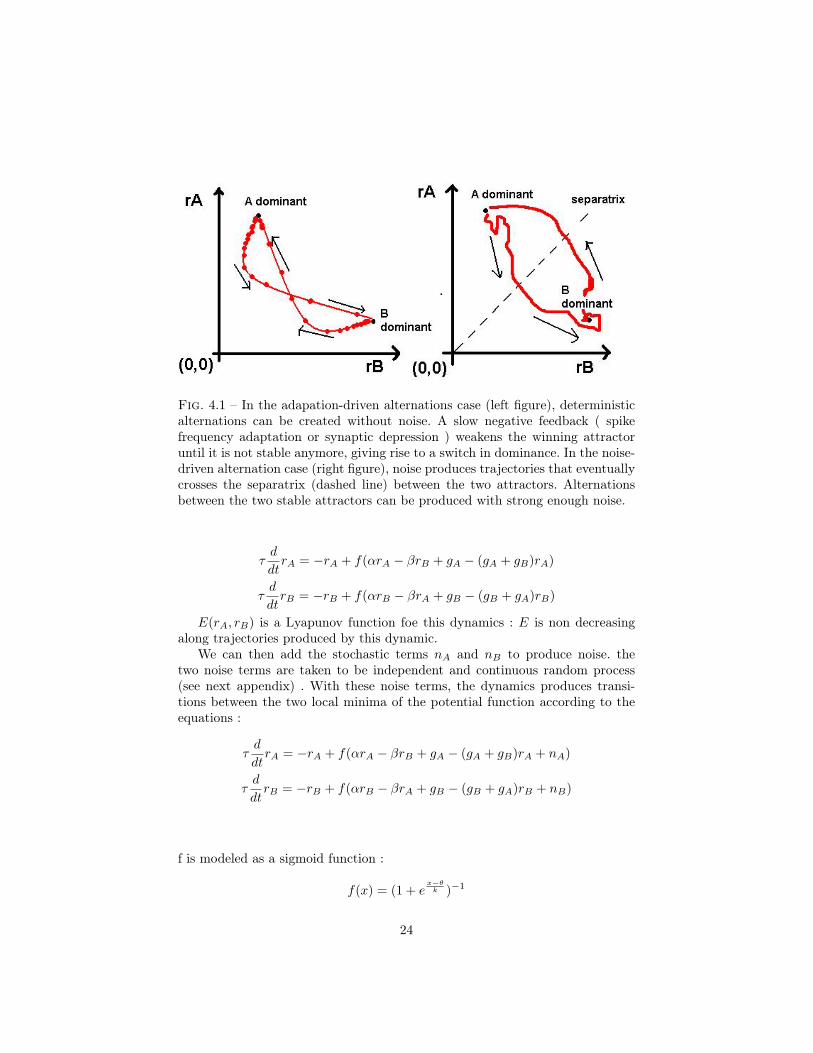
Fig. 4.1 – In the adapation-driven alternations case (left figure), deterministicalternations can be created without noise. A slow negative feedback ( spikefrequency adaptation or synaptic depression ) weakens the winning attractoruntil it is not stable anymore, giving rise to a switch in dominance. In the noise-driven alternation case (right figure), noise produces trajectories that eventuallycrosses the separatrix (dashed line) between the two attractors. Alternationsbetween the two stable attractors can be produced with strong enough noise.

τd

dtrA = −rA + f(αrA − βrB + gA − (gA + gB)rA)

τd

dtrB = −rB + f(αrB − βrA + gB − (gB + gA)rB)

E(rA, rB) is a Lyapunov function foe this dynamics : E is non decreasingalong trajectories produced by this dynamic.

We can then add the stochastic terms nA and nB to produce noise. thetwo noise terms are taken to be independent and continuous random process(see next appendix) . With these noise terms, the dynamics produces transi-tions between the two local minima of the potential function according to theequations :

τd

dtrA = −rA + f(αrA − βrB + gA − (gA + gB)rA + nA)

τd

dtrB = −rB + f(αrB − βrA + gB − (gB + gA)rB + nB)

f is modeled as a sigmoid function :

f(x) = (1 + ex−θ

k )−1

24

with threshold θ = 0.1 and k = 0.05.

4.0.7 noiseThe noise used here is an Ornstein-Uhlenbeck process with zero mean and

deviation σ.d

dtn = − n

τs+ σ

√2τs

ξ(t)

Where ξ(t) is a white noise process with zero mean and < ξ(t1)ξ(t2) >=δ(t1−t2) . τs = 100ms is taken to be 10 times slower than the network dynamics( τ = 10ms).

4.0.8 synaptic facilitation and depressionIn the second model for persistence, we modelise the evolution of the recur-

rent excitation factor α in the following way :

α = α(1 + δ)

Where δ evolves over time and is always positive. δ = δon + δoff , when thecoressponding population is active, δ = δon, when the corresponding populationis inactive : δ = δoff .

δon undergoes a quick increase and then a slow decay. We modelize it by :δon = δup − δdown and

˙δup = (shift− δon)/τup

˙δdown = (shift− δdown)/τdown

δoff slowly decays toward zero :

˙δoff = (−δoff )/τoff

We the population becomes active again, the value of shift is redefined asthe last value of delta +0.05. The three different time scales used here are :τup = 0.05 sec , τdown = 2.00 sec and τoff = 20.0 sec .

25