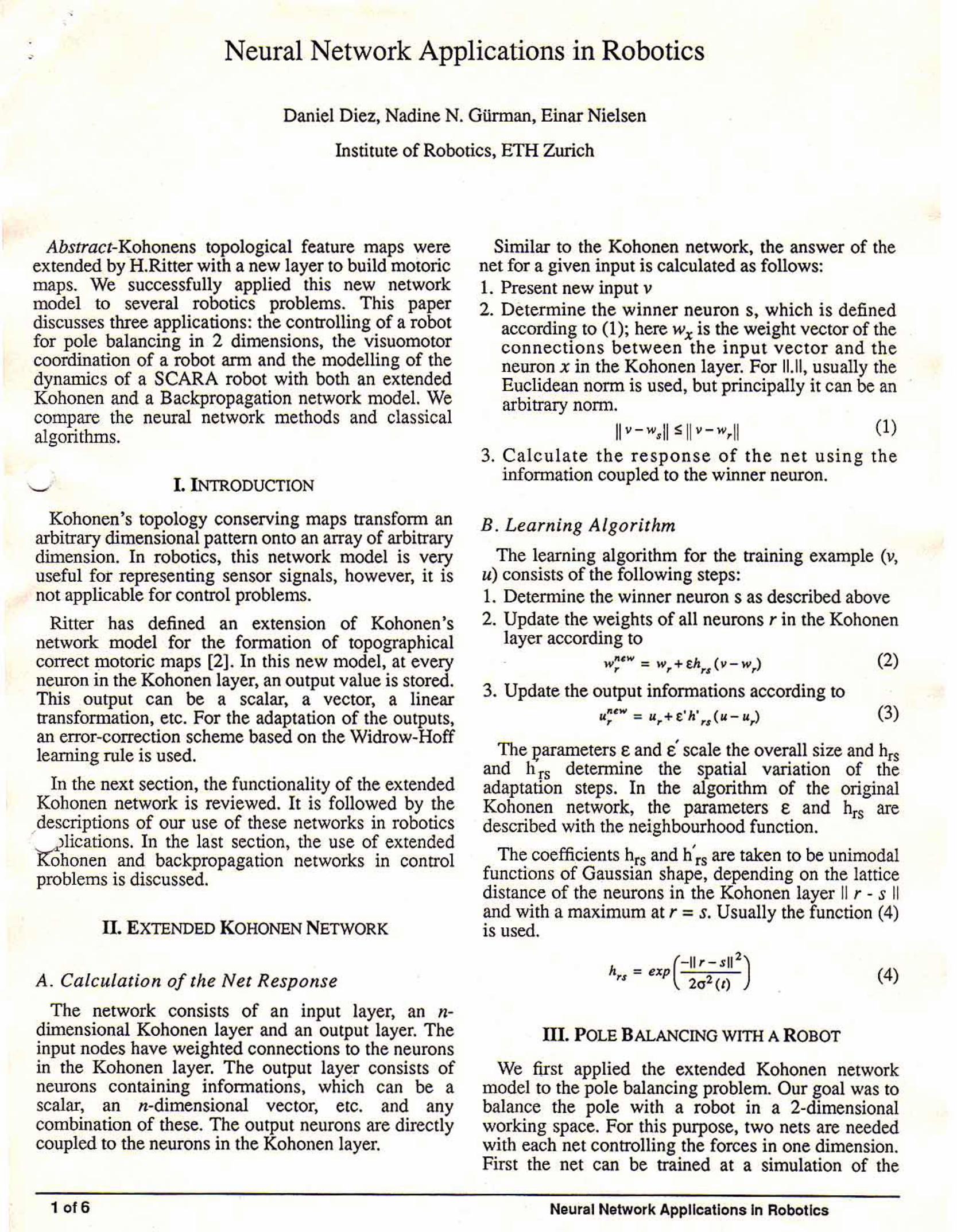
Neural Network Applications in Robotics

Neural Network Applications in Robotics

Daniel Diez, Nadine N. Günnan, Einar Nielsen

Institute of Robotics, ETH Zurich

Abstract-Kohonens topological feature maps were extended by H.Ritter with a new layer to build motoric maps. We successfully applied this new network model to several robotics problems. This paper discusses three applications: the Controlling of a robot for pole balancing in 2 dimensions, the visuomotor coordination of a robot arm and the modelling of the dynamics of a SCARA robot with both an extended Kohonen and a Backpropagation network model. We compare the neural network methods and classical algorithms.

I. INTRODUCTION

Kohonen's topology conserving maps transform an arbitrary dimensional pattern onto an array of arbitrary dimension. In robotics, this network model is very useful for representing sensor signals, however, it is not applicable for control problems.

Ritter has defined an extension of Kohonen 's network model for the formation of topographical correct QJOtoric maps [2]. In this new model, at every neuron in the Kohonen layer, an output value is stored. This output can be a scalar, a vector, a linear transformation, etc. For the adaptation of the outputs, an error-correction scheme based on the Widrew-Hoff learning rule is used.

In the next section, the functionality of the extended Kohonen network is reviewed. It is followed by the descriptions of our use of these networks in robotics

' Jlications. In the last section, the use of extended ~honen and backpropagation networks in control problems is discussed.

li. EXTENDED KORONEN NETWORK

A. Calculation of the Net Response

The network consists of an input layer, an n­dimensional Kohonen layer and an output layer. The input nodes have weighted connections to the neurons in the Kohonen layer. The output layer consists of neurons containing informations, which can be a scalar, an n-dimensional vector, etc. and any combination of these. The output neurons are directly coupled to the neurons in the Kohonen layer.

1 of6

Similar to the Kohonen network, the answer of the net for a given input is calculated as follows: 1. Present new input v 2. Determine the winner neuron s, which is defined

according to (1); here wx is the weight vector of the connections between the input vector and the neuron x in the Kohonen layer. For 11.11, usually the Euclidean norm is used, but principally it can be an arbitrary norm.

Uv-wsiiSIIv-w,. ll (1)

3. Calculate the response of the net using the information coupled to the winner neuron.

B. Learning Algorithm

The learning algorithm for the training example (v, u) consists of the following steps: 1. Determine the winner neuron s as described above 2. Update the weights of all neurons r in the Kohonen

layer according to WIICW: W +W (V-W}

T T TS T (2)

3. Update the output infonnations according to /ICW 'h' ( ) UT : U,. + t I'S U- U,. (3)

The 1?arameters e and e' scale the overall size and hrs and h rs determine the spatial variation of the adaptation steps. In the algorithm of the original Kohonen network, the parameters e and hrs are described with the neighbourhood function.

The coefficients hrs and h'rs are taken tobe unimodal functions of Gaussian shape, depending on the lattice distance of the neurons in the Kohonen layer II r - s II and with a maximum at r = s. Usually the function (4) is used.

h = ex (-II r-sllz) rs P 2a2 (t) (4)

ill. POLE BALANCING WITH A ROBOT

We first applied the extended Kohonen network model to the pole balancing problem. Our goal was to balance the pole with a robot in a 2-dimensional working space. For this purpose, two nets are needed with each net controlling the forces in one dimension. First the net can be trained at a Simulation of the

Neural Network Appllcatlons ln Robotlcs

: system, but afterwards an on-line training at the real system is needed, because the model the simulation is based upon, is always inexact. As the acceleration of the robot required to balance the pole cannot be measured at the system, an unsupervised training strategy has to be used.

Among the several possibilities for applying inputs to the network, the simplest one is to take two consecutive angles <p(t-1) and <p(t) between the pole and the vertical axis. The output of the net is the force v required at the bottom of the pole to minimize the <p. The output nodes r contain also the parameter ar which defines the region ,to be searched for a new force and the grading value br achieved with the force vr The grading function is defined with the equation (5). During the training phase, for an inputpair [<p(t-1) and <p(t)] first the winner node s is calculated; the force as an output ofthe net is defined with (6), where 11 is a random value with 0 < 11 < 1.

R(q>) == -q>2 (5)

f,. = v .. +as1'\ (6) The net output fn is applied to the system and the

--._}provement in the grading is calculated. If this value 1s better than the grading bs achieved with the old force v s• the output v of s and its neighbours are modified due to equation (3). Each time the neuron s is selected, the parameter a of itself and its neighbours is modified with (7) to reduce the size of the region to be looked for a new force value in the next learning step.

' a~ew = a~ld + E." h" rs ( a- a~ld) (7)

The modification of the winner neurons grading value b8 is done according to equation (8).

b:ew = b~ld + l' (AR - b~ld) (8)

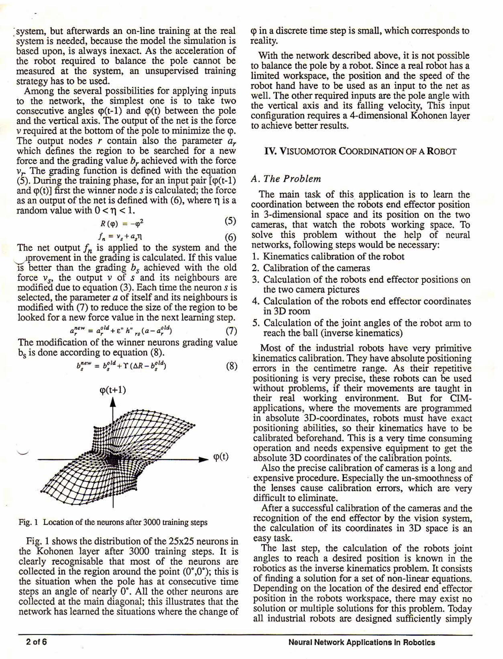
<p(t+1)

Fig. 1 Location of the neurons after 3000 training steps

Fig. 1 shows the distribution of the 25x25 neurons in the Kohonen layer after 3000 training steps. It is clearly rec.ognisable that most of the neurons are collected in the region around the point co· ,o·); this is the Situation when the pole has at consecutive time steps an angle of nearly o·. All the other neurons are collected at the main diagonal; this illustrates that the network has learned the Situations where the change of

2 of6

cp in a discrete time step is small, which corresponds to reality.

With the network described above, it is not possible to balance the pole by a robot. Since a real robot has a limited workspace, the position and the speed of the robot hand have to be used as an input to the net as weiL The other required inputs are the pole angle with the vertical axis and its falling velocity, This input con:figuration requires a 4-dimensional Kohonen layer to achieve better results.

IV. VISUOMOTOR COORDINATION OF A ROBOT

A. The Problem

The main task of this. application is to learn the coordination between the robots end effector position in 3-dimensional space and its position on the two cameras, that watch the robots working space. To solve this problern without the help of neural networks, following_ steps would be necessary: 1. Kinematics calibration of the robot 2. Calibration of the cameras 3. Calculation of the robots end effector positions on

the two camera pictures 4. Calculation of the robots end effector coordinates

in 3D room 5. Calculation of the joint angles of the robot arm to

reach the ball (inverse kinematics)

Most of the industrial robots have very primitive kinematics calibration. They have absolute positioning errors in the centimetre range. As their repetitive positioning is very precise, these robots can be used without problems, if their movements are taught in their real working environment. But for CIM­applications, where the movements are progranuned in absolute 3D-coordinates, robots must have exact positioning abilities, so their kinematics have to be calibrated beforehand. This is a very time consuming operation and needs expensive equipment to get the absolute 3D coordinates ofthe calibration points.

Also the precise calibration of cameras is a long and · expensive procedure. Especially the un-smoothness of

the Jenses cause calibration errors, which are very difficult to eliminate.

After a successful calibration of the cameras and the recognition of the end effector by the vision system, the calculation of its coordinates in 3D space is an easy task.

The last step, the calculation of the robots joint angles to reach a desired position is known in the robotics as the inverse kinematics problem. It consists of finding a solution for a set of non-linear equations. Depending on the location of the desired end effector position in the robots workspace, there may exist no solution or multiple solutions for this problem. Today a11 industrial robots are designed sufficiently simply

Neural Network Appllcations ln Robotlcs

·so that their inverse kinematics can be calculated with analytic methods.

B. The model

I~ our experiments, two cameras watch a 30x30x30 cm area of the robot working space. The robot learns to grip a pingpongball which is hold anywhere in this area. To make the task of object recognition easier, the ball contains a bulb and the cameras are faded so that only the light spot appears on the pictures. This makes it possible to work with the system in a room with normal light conditions. For the recognition of the light spot, a special vision system is used, which has been developed at the Institute for Robotics, ETH Zurich, for the pingpong playing robot; it can recognize round objects, lik.e a pingpongball or a light spot in real time.

The robot used is a Mitsubishi RV-Ml, a 5-axis robot with a small working space. Its absolute positioning errors in the middle of its working space are so minimal that they are not measurable without · -.ecial equipment. In the near of its working space

't:7()rders, however, these errors are up to two centimetres.

Both the vision system and the robot are controlled from a Sun Spare workstation. They both are attached at the RS-232 ports of the workstation. The low level programs for Controlling the ports are written in C, and the high Ievel programs like the neural network Simulator are written in Modula-2.

C. Extended Kohonen Network Model

The input to the network is a four-dimensional vector u, which contains the two 2-dimensional coordinate vectors u 1 and u2 representing the position of the pingpong ball on the two camera pictures.

The outputs of the network are a n-dimensional vector S and a nx4 matrix A. S contains the joint ~ngles of the n-axis-robot. A represents the Jacobian "--'4trix. If neuron s is the winner, the joint angles of the robot to grip the ball are calculated with (9).

(9) .

The net is trained in two phases: First it is trained with a Simulation and afterwards it is trained at the real system. The first phase is needed because the on­line training at the robot is slow and superfluous; it is enough to have an inexact simulation of the system consisting of the robot and the two cameras. During the first phase the net learns the simulated model which contains the most important global dependencies. In the second phase the net is trained at the real system, so it learns the exact transformation between the ball positions on the two camera pictures and the robot joint angles.

3of6

Before starring with the first training phase, robot and camera geometry and their positions referring to a predefined base coordinate system are measured. With these data the system is simulated to produce the required training informations. The training time of the second phase is dependent on the precision of these measurements.

D. The learning algorithm

The net is initialized randomly. The training algorithm for one step is as follows: 1. Make a random movement with the robot. Its loca­

tion on the cameras defines the input u to the net. 2. The winner node s delivers the informations S8 and

As. . 3. Adjust the weights of all neurons r with (2). 4. Move robot with the information 9 8 to get the

position vi on the cameras 5. Recalculate the joint information with (9) and make

the movement with the new joint angles; the robots location on the cameras after this fine movement is Vf

6. Calculate the new values for S and A with

A'~ = As+llvrv;I!2A,(u-w8 - vrv;) (vrv;)T

(B,A)~ew = (B,A)~1d+e'h,s((9,A)v- (B,A)~1d)

E. Results

(10)

(11)

(12)

Due to the topography of the working space, a 3-dimensional Kohonen layer net has been used for the problern of the visuomotor cfordination. For a working space of 30x30x30 cm , a net with 8x8x8 neurons has delivered satisfactory results. Of course, the precision of the results can be improved by taking more neurons, but this would mean Ionger training times and memory waste. A similar improvement can also be achieved by making an interpolation between the result of the winner neuron and its neighbour neurons.

The training parameters for the first phase are the same as suggested . in Ritter [2]. For the on-line training, the choice of the parameter depends on the quality of the net obtained in the first phase. If the precision of the net for gripping the ball is good, the parameters defining the neighbourhood function are taken so that for each training example only one neuron is adjusted. In this case only 100 - 500 training steps are necessary. If however the positioning errors of the ne.t are more than 1 cm., this is the case, if the net is trained at a model with .measurement errors of I cm and more, the net is trained with the same parameter values as in the first phase for up to 1000 steps.

Neural Network Appllcations ln Robotlcs

• . •

V. MODELING THE DYNAMICS OF A ROBOT

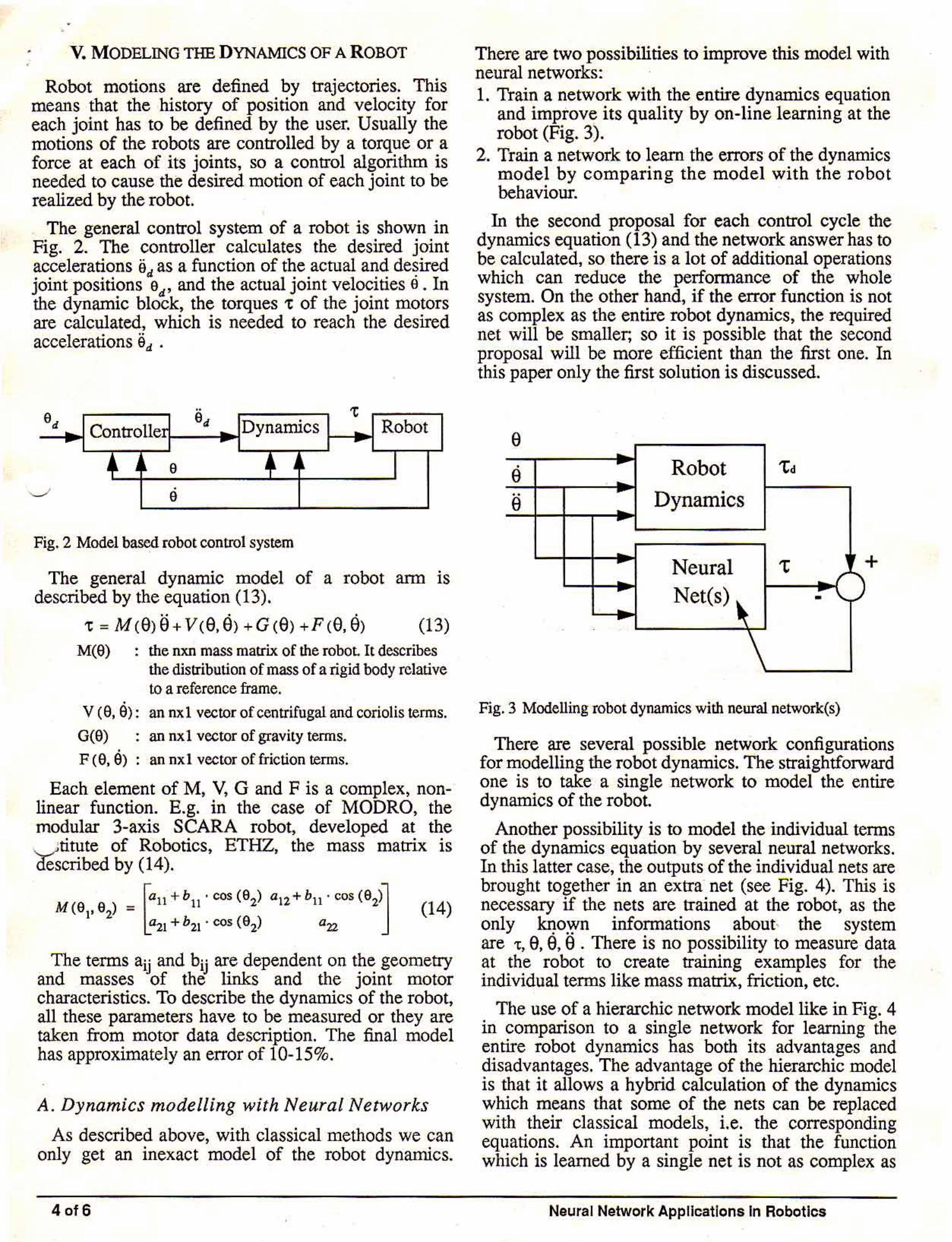
Robot motions are defined by trajectories. This means · that the history of position and velocity for each joint has tobe defined by the user. Usually the motions of the robots are controlled by a torque or a force at each of its joints, so a control algorithm is needed to cause the desired motion of each joint to be realized by the robot.

The general control system of a robot is shown in Fig. 2. The controller calculates the desired joint accelerations öd as a function of the actual and desired jofurpositions ed, and the actual joint velocities e. In the dynamic block, the torques 't of the joint motors are calculated, which is needed to reach the desired accelerations öd .

•• 't ed ed Controllet Dynamics Robot .. .. .. ... • •

j • e ' ~ ' ~ . e

Fig. 2 Model based robot control system

The general dynarnic model of a robot arm is described by the equation (13).

t=M<8>El+V(8,S)+G(8)+F<8.S) (13) M(e) : the nxn mass matrix of the robot It describes

•

the distribution of mass of a rigid body relative to a reference frame .

V (e, e): an nxl vector of centrifugal and coriolis terms.

G(e) : an nxl vector of gravity terms.

F (e, E)) : an nxl vector of friction terms.

Each element of M, V, G and F is a complex, non­linear function. E.g. in the case of MODRO, the mo~ular 3-axis S~ARA robot, developed at the v ntute of Roboncs, ETHZ, the mass matrix is described by (14).

T he terms aij and bij are dependent on the geometry and masses of the links and the joint motor characteristics. To describe the dynamics of the robot, all these parameters have to be measured or they are taken from motor data description. The final model has approximately an error of 10-15%.

A. Dynamics modelling with Neural Networks

As described above, with classical methods we can only get an inexact model of the robot dynamics.

4 of6

There are two possibilities to improve this model with neural networks: · 1. Train a network with the entire dynamics equation

and imptove its quality by on-line learning at the robot (Fig. 3).

2. Train a network to learn the errors of the dynamics model by comparing the model with the robot behaviour.

In the second proposal for each control cycle the dynamics equation (13) and the network answer has to be calculated, so there is a lot of additional operations which can reduce the perfonnance of the whole system. On the other hand, if the error function is not as complex as the entire robot dynamics, the required net will be smaller; so it is possible that the second proposal w.ill be more ef:ficient than the first one. In this paper only the first solution is discussed.

e .. • Robot 'td e -

•• e • Dynami es -• - , Ir • Neural 't + - • -..

Net(s)' .. --• .

\ Fig. 3 Modelling robot dynamics with neural network(s)

There are several possible network configurations for ~odelling the r?bot dynamics. The straighttorward one 1s to take a smgle network to model the entire dynamics of the robot

Another possibility is to model the individual terms of the dynarnics equation by several neural networks. In this latter case, the Outputs of the individual nets are brought together in an extra· net (see Fig. 4). This is necessary · if the nets are trained at the robot, as the only kqo:'?'n infonnations about, the system are 't, e, e. e . There is no possibility to measure-data ~t ~h~ robot to . create training examples for · the mdivtdual terms like mass matrix, friction, etc.

. The use ?f a hierarc~c network modellike in Fig. 4 m companson to a smgle network for learning the e~tire robot dynamics has both its advantages and d1sadvantages. The advantage of the hierarchic model is that it allows a hybrid calculation of the dynamics w~ch m~ans th~t some of th~ nets can be replaced w1th .the1r clas~1cal models •. 1.e: the corresponding equat10ns. An 1mportant pomt 1s that the function which is Iearned by a single net is not as complex as

Neural Network Applicatlons ln Robotlcs

•

-the full dynamics function, so the net dimension is · small and the net can learn the function more precisely with less training examples. The disadvantage can be its efficiency; the net modelling the whole dynamics is much bigger than the single nets in the hierarchic net model, but in the whole its number of neurons is smaller.

ANN

ANN ANN ANN ANN

' .. ' e e e e e e e

Fig. 4 Hierarchie network model for modelling robot dynamics

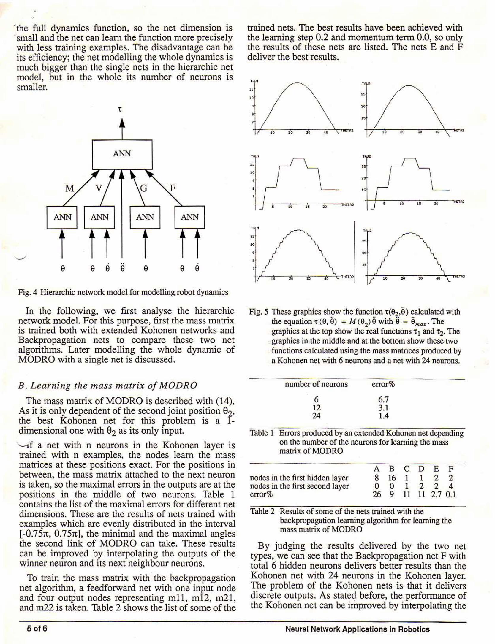
In the following, we first analyse the hierarchic network model. For this purpose, first the mass matrix is trained both with extended Kohonen networks and Backpropagation nets to compare these two net algorithms. Later modelling the whole dynamic of MODRO with a single net is discussed.

B . Learning the mass matrix of MODRO

The mass matrix ofMODRO is described with (14). As it is only dependent of the second joint position 92, the best Kohonen net for this problern is a I­dimensional one with 82 as its only input.

'-if a net with n neurons in the Kohonen layer is trained with n examples, the nodes learn the mass matrices at these positions exact. For the positions in between, the mass matrix attached to the next neuron is taken, so the maximal errors in the outputs are at the positions in the middle of two neurons. Table 1 contains the list of the maximal errors for different net dimensions. These are the results of nets trained with examples which are evenly distributed in the interval [-0.751t, 0.751t], the minimal and the maximal angles the second link of MODRO can take. These results can be improved by interpolating the outputs of the winner neuron and its next neighbour neurons.

To train the mass matrix with the backpropagation net algorithm, a feedforward net with one input node and four output nodes representing mll, m12, m21, and m22 is taken. Table 2 shows the list of some of the

5 of 6

trained nets. The best results have been achieved with the learning step 0.2 and momentum term 0.0, so only the results of these nets are listed. The nets E and F deliver the best results.

T 1

10

• • ,I

+f---..,.,10--:

2-:-0

- ,"C!:-0 --,o:40~"Tl<:E:TR2

l \ H

10

' • 1

...J 5 10 15 ..

T .. 10

• 8

7

10 IVA2

" f'2 I \ 25

20

15

• ,o " 20 ~·~ .J

T 2

25

20 .. 20 "' 40

EU2

Fig. 5 These graphics show the function t(e2,ä) calculated with the equation 't (9, Ö) = M (92) ä with ä = ämax. The graphics at the top show the real functtons t 1 and 't:z. The graphics in the middle.and at the bottom show these two functions calculated using the mass matrices produced by a Kohonen net with 6 neurons and a net with 24 neurons.

number of neurons

6 12 24

error%

6.7 3.1 1.4

Table 1 Errors produced by an extended Kohonen net depending on the number of the neurons for learning the mass matrix ofMODRO

nodes in the first hidden Jayer nodes in the first second layer error%

A B C D 8 16 1 1 0 0 1 2 26 9 11 11

E F 2 2 2 4

2.7 0.1

Table 2 Results of some of the nets trained with the backpropagation learning algorithm for learning the mass matrix of MODRO

By judging the results delivered by the two net types, we can see that the Backpropagation net F with total 6 hidden neurons delivers better results than tbe Kohonen net with 24 neurons in the Kohonen layer. The problern of the Kohonen nets is that it delivers discrete outputs. As stated before, the performance of the Kohonen net can be improved by interpolating the

Neural Network Appllcations in Robotlcs

~outputs. With a linear interpolation the errors can be 'halved. With better interpolation ·methods, the error can furtherbe reduced massively.

In the last section these two network models are discussed and compared in more detail.

C. Learning the Dynamics of MODRO

The dynamics equation of MODRO has 6 variables, so a 6~dimensional Kohonen network is required to learn this function with conserving the topological information in the net.

For learning the whole dynamics ofMODRO with a backpropagation net, there are several possibilities for choosing the inputs. 1. Positions, velocities and accelerations 9, ä, ä of

the joints 2. Several non-linear tenns which are hidden in the

dynamics equation (13): Sign <Eh, Sin (9), Cos (9) etc.

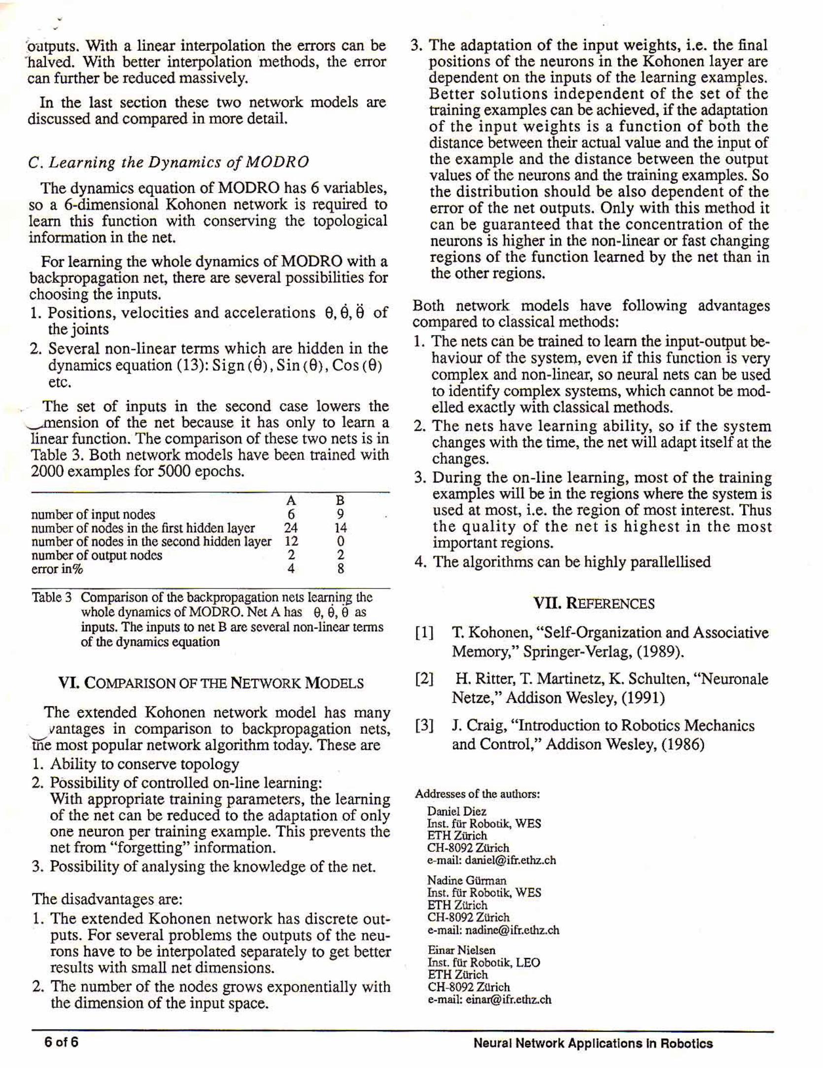
The set of inputs in the second case lowers the ..._...mension of the net because it has only to learn a linear function. The comparison of these two nets is in Table 3. Both network models have been trained with 2000 examples for 5000 epochs.

A B number of input nodes 6 9 number of nodes in the first hidden Iayer 24 14 number of nodes in the second hidden layer 12 0 number of output nodes 2 2 errorin% 4 8

Table 3 Comparison of the backpropagation nets lea!'l!i~g the whole dynamics of MODRO. Net A has e, e, e as inputs. The inputs to net B are several non-linear terms of the dynarnics equation

VI. COJ.\.1PARISON OF Tiffi NETWORK MODELS

The extended Kohonen network model has many . vantages in comparison to backpropagation nets, 'ule most popular network algorithm today. These are 1. Ability to conserve topology 2. Pössibility of controlled on-line learning:

With appropriate training parameters, the learning of the net can be reduced to the adaptation .of only one neuron per training example. This prevents the net from "forgetting" infonnation.

3. Possibility of analysing the knowledge of the net.

The disadvantages are: 1. The extended Kohonen network has discrete out­

puts. For several problems the outputs of the neu­rons have to be interpolated separately to get better results with small net dimensions.

2. The nurober of the nodes grows exponentially with the dimension of the input space.

6 of6

3. The adaptation of the input weights, i.e. the final positions of the neurons in the Kohonen layer are dependent on the inputs of the learning examples. Better solutions independent of the set of the training examples can be achieved, if the adaptation of the input weights is a function of both the distance between their actual value and the input of the example and the distance between the output values of the neurons and the training examples. So the distribution should be also dependent of the error of the net outputs. Only with this method it can be guaranteed that the concentration of the neurons is higher in the non-linear or fast changing regions of the function learned by the net than in the other regions.

Both network models have following advantages compared to chtssical methods: 1. The nets can be trained to learn the input-output be­

haviour of the system, even if this function is very complex and non-linear, so neural nets can be used to identify complex systems, which cannot be mod­elled exactly with classical methods .

2. The nets have learning ability, so if the system changes with the time, the net will adapt itself at the changes.

3. During the on-line learning, most of the training examples will be in the regions where the system is used at most, i.e. the region of most interest. Thus the quality of the net is highest in the most important regions.

4. The algorithms can be highly parallellised

VII. REFERENCES

[1] T. Kohonen, "Self-Organization and Associative Memory," Springer-Verlag, (1989).

[2] H. Ritter, T. Martinetz, K. Schulten, "Neuronale Netze," Addison Wesley, (1991)

[3] J. Craig, "Introduction to Robotics Mechanics and Control," Addison Wesley, (1986)

Addresses of the authors: Daniel Diez Inst. für Robotik, WES ETHZürich CH-8092 Zürich e-mail: [email protected]

Nadine Gllnnan Inst. fllr Robotik, WES ETH Zllrich CH-8092 Zürich e-mail: [email protected]

Einar Nielsen Inst. für Robotik, LEO ETHZürich CH-8092 Zürich e-mail: [email protected]

Neural Network Appllcations ln Robotlcs