Network Potentials

Bonn E on Dis ussion PapersDiscussion Paper 28/2005

Network Potentials

by

Subhadip Chakrabarti, Robert P. Gilles

October 2005

Bonn Graduate S hool of E onomi sDepartment of E onomi sUniversity of BonnAdenauerallee 24 - 42D-53113 Bonn

The Bonn Graduate School of Economics is sponsored by the

Network Potentials∗

Subhadip Chakrabarti† Robert P. Gilles‡

October 2005

Abstract

A network payoff function assigns a utility to all participants in a (social) net-work. In this paper we discuss properties of such network payoff functions thatguarantee the existence of certain types of pairwise stable networks and the con-vergence of certain network formation processes. In particular we investigatenetwork payoff functions that admit an exact network potential or an ordinalnetwork potential. We relate these network potentials to exact and ordinal po-tentials of a non-cooperative network formation game based on consent in linkformation. Our main results extend and strengthen the current insights in theliterature on game theoretic approaches to social network formation.

Keywords: Network formation; pairwise stability; potential functions.

JEL Classification: C72, C79, D85.

∗We thank Matt Jackson and Sudipta Sarangi for extensive discussions on the subject of this paper.For downloadable PDF files of several of the cited papers we refer to the corresponding author’s website at http://gilles.economics-network.org.

†Department of Economics, Queen’s University, Belfast, Northern Ireland, UK. Email :[email protected]. Part of this research was done while this author was at Bonn on a post-doctoralresearch fellowship. We thank the Department of Economics at the University of Bonn for their hospi-tality and financial support.

‡Corresponding author. Address: Department of Economics, Virginia Tech (0316), Blacksburg, VA24061, USA. Email : [email protected]. Part of this research was done at the Center for Economic Researchat Tilburg University, Tilburg, the Netherlands. Financial support from the Netherlands Organizationfor Scientific Research (NWO), grant # 46-550, is gratefully acknowledged.

1 Introduction

Since the introduction of the notion of pairwise stability in Jackson and Wolinsky

(1996), one of the main research questions that have been investigated in the litera-

ture on social network formation, has been the problem of the existence of (strictly)

pairwise stable networks. A related question is whether certain network formation

processes converge to these types of stable networks. Preliminary investigation of

these issues was addressed in Jackson and Watts (2001) and Jackson and Watts

(2002b). Here we investigate the fundamental properties of network payoff struc-

tures that bear on these two fundamental problems. We show that the admittance

of (ordinal) network potential functions provides a powerful tool that satisfactorily

resolves these fundamental problems.

We consider undirected social networks, which are founded on the principle that

each link is between two equally participating players. Hence, both players are as-

sumed to consent voluntarily and in full knowledge to the formation of a link between

them.1 This idea was first formalized by Myerson (1991, page 448) as a normal form

game—referred to as the “Consent Game”. Myerson’s Consent Game and its vari-

ations unfortunately admit a multitude of Nash equilibria as pointed out in Dutta,

van den Nouweland, and Tijs (1998), Jackson (2005b), and Gilles, Chakrabarti, and

Sarangi (2005a). From this rather unsatisfactory fact, there emerged two alternative

theories of network formation under consent.

In their seminal paper Jackson and Wolinsky (1996) introduced a link-based ap-

proach to network formation. The central strategic concept is now the link rather

than the players between whom this link is formed. In particular, they defined the

link-based notion of pairwise stability as an alternative description of the require-

ment of consent in link formation. This alternative formulation of stability reduces

the multitude of acceptable networks. Existence of pairwise stable networks and the

convergence of simple link-based improvement processes to such pairwise stable net-

works has been addressed in Jackson and Watts (2001), Jackson and Watts (2002a),

and Jackson and Watts (2002b).

The other approach to resolve the problem of the indeterminacy of Myerson’s

Consent Game is to consider network-based refinements of the Nash equilibrium con-

cepts within the context of Myerson’s Consent Game and its variations. This has been

pursued by Gilles, Chakrabarti, and Sarangi (2005a) and Gilles and Sarangi (2005a)

1The alternative is to consider directed social networks, in which links are formed without the con-sent of one of the players. We refer to Bala and Goyal (2000) and related subsequent work for a studyof these so-called Nash networks.

1

for the case that the formation of links is costly. Gilles and Sarangi (2005a) con-

sider myopic learning processes based on the formation of simple belief systems. In

these belief systems a player formulates expectations about whether other players

would consent to forming links with her. Each player now formulates a best response

to her formed myopic beliefs. This learning process only converges satisfactorily if

the formed beliefs are confirmed within the stable state that is reached. Gilles and

Sarangi show that the resulting set of these so-called self-confirming equilibria gen-

erate a strict subset of the class of pairwise stable networks, the so-called strictlypairwise stable networks. Gilles and Sarangi (2005a) do not address under which

conditions such strictly pairwise stable networks exist.

Here we show that if the network payoff function admits a potential function, the

existence of such strictly pairwise stable networks is guaranteed and, therefore, that

the learning processes based on the formation of the myopic belief systems intro-

duced by Gilles and Sarangi (2005a) indeed converge to self-confirming equilibrium

networks. Furthermore we explore the relationship of these network potentials with

the improvement processes discussed by Jackson and Watts (2002a).

Two seminal contributions to the game theoretic literature address the introduc-

tion of potential functions into the analysis of cooperative as well as non-cooperative

games. These potential functions were seminally introduced by Hart and Mas-Colell

(1989) for cooperative games and by Monderer and Shapley (1996) for non-coopera-

tive games. Hart and Mas-Colell showed the fundamental relationship between

their cooperative potential function and the Shapley value for cooperative games.

(Shapley 1953) Monderer and Shapley and subsequent contributions showed that

non-cooperative games admitting potentials are closely related to congestion games

in the sense of Rosenthal (1973). These two strands of the literature were brought

together by Qin (1996) and especially Ui (2000), who showed that the payoff func-

tions in non-cooperative potential games are the Shapley values of a corresponding

class of cooperative games. These fundamental insights showed that there is a strong

relationship between the various classes of non-cooperative potential games and Hart

and Mas-Colell’s cooperative potential theory.

In the present paper we introduce potential functions for a broad class of net-

work payoff functions as descriptors of network formation fundamentals. First, we

consider exact network potentials, which assign the marginal contributions of newly

formed links to the participants in the network. The class of network payoff functions

for which such exact network potentials can be considered are exactly those network

payoff functions that satisfy Myerson (1977)’s “fairness” property—more recently re-

formulated as an equal bargaining power property. (Jackson and Wolinsky 1996, page

2

54) We show that a network payoff function admits an exact network potential if and

only if Myerson’s Consent Game admits a game-theoretic exact potential in the sense

of Monderer and Shapley (1996). Furthermore, we extend Qin (1996)’s equivalence

theorem by showing that, if a network payoff function admits such an exact network

potential, the network payoffs correspond in fact to the Shapley values of a certain

class of related cooperative games.

The presence of an exact network potential is a rather demanding property. It

is natural to weaken this requirement to that of the admittance of an ordinal net-

work potential function. We show that the presence of an ordinal network potential

is a strictly weaker requirement than Myerson’s Consent Game admitting a game-

theoretic ordinal potential in the sense of Monderer and Shapley (1996).

The main consequence of the presence of an ordinal potential is to guarantee the

convergence of network formation processes based on myopic payoff improvements

as introduced in Jackson and Watts (2002a) and the existence of strictly pairwise sta-

ble networks. In particular, if the network payoff function admits an ordinal network

potential, such network formation processes based on myopic payoff improvements

are shown to converge to pairwise stable networks. This generalizes the main result

in Jackson and Watts (2001). Furthermore, if Myerson’s Consent Game admits an or-

dinal potential, there exists at least one strictly pairwise stable network in the sense

of Gilles and Sarangi (2005a).

It should be clear from the developed insights in this paper that the concept of a

network potential is a very powerful one. It allows the two main questions regarding

the existence of (strictly) pairwise stable networks and the convergence of certain

network formation processes to be fully resolved.

The rest of the paper is organized as follows. Section 2 introduces terminology, the

notation and the basic network formation theories. In section 3, we define exact

network potentials and their relation with the exact potentials of the Consent Game

introduced by Myerson (1991, page 448). In Section 4, we define ordinal network

potentials and their relationship with ordinal potentials of Myerson’s Consent Game.

In Section 5, we show that certain classes of network formation games admitting (or-

dinal) potentials allow the convergence of network formation processes to pairwise

stable networks and guarantee the existence of a strictly pairwise stable network, thus

linking this research to work on network formation based on myopic belief systems.

(Gilles and Sarangi 2005a) In Section 6 we look at some applications of potential

functions and some special properties of these classes of network formation games.

Section 7 concludes.

3

2 Preliminaries

In this section we discuss required material from non-cooperative game, cooperative

game, the theory of game theoretic potentials, and network formation theory.

2.1 Non-cooperative games and potentials

A non-cooperative game on a fixed, finite player set N = {1, . . . , n} is given by a list

(A,π) = (Ai, πi)i∈N where for every player i ∈ N, Ai denotes an action set and

πi : A → R denotes player i’s payoff function with A = A1 × A2 × · · · × An. An

individual action of player i ∈ N is denoted by ai ∈ Ai and an action tuple is written

as a = (a1, a2, . . . , an) ∈ A. For every action tuple a ∈ A and player i ∈ N, we

denote by a−i = (a1, a2, . . . , ai−1, ai+1, . . . , an) ∈ A−i =∏j6=iAj as the actions

selected by players other than i. π = (π1, π2, . . . , πn) : A → RN is the composite

payoff function of this game.

Throughout this paper, we denote a non-cooperative game for short by the pair

(A,π). A non-cooperative game is finite if for every i ∈ N, the action set Ai is finite.

In this paper, we only apply finite games.

An action set ai ∈ Ai for player i ∈ N is a best response to a−i ∈ A−i if for

every action bi ∈ Ai we have that πi(ai, a−i) > πi(bi, a−i). An action-tuple (strategy

profile) a∗ ∈ A is a Nash equilibrium of the game (A,π) if for every player i ∈ N the

action ai is a best response to a−i, i.e., for every action bi ∈ Ai we have πi(a∗) >

πi(bi, a∗−i).

We denote a−i,j = (a1, a2, . . . , ai−1, ai+1, . . . , aj−1, aj+1, . . . , an) ∈ A−i,j, where

A−i,j =∏k6=i,j

Ak

is the actions selected by players other than i and j. Further, a−i,j = a−j,i.

A function Q : A → R is an exact potential of the non-cooperative game (A,π) on the

player set N if for every player i ∈ N, action tuple a ∈ A and action bi ∈ Ai,

πi(a) − πi(bi, a−i) = Q(a) −Q(bi, a−i). (1)

The notion of a game theoretic (exact) potential was seminally introduced in Mon-

derer and Shapley (1996). The potential provides a very strong relationship between

the various strategy tuples in the game; it “directs” the game towards its Nash equi-

libria (in pure strategies). Games that admit exact potentials have very powerful

4

properties, including the guaranteed existence of a Nash equilibrium in pure strate-

gies and the convergence of any improving dynamic improvement process to a Nash

equilibrium in a finite number of steps.

A function Q : A → R is an ordinal potential of the non-cooperative game (A,π)

on the player set N if for every player i ∈ N, action tuple a ∈ A and action bi ∈ Ai,

πi(a) − πi(bi, a−i) > 0 if and only if Q(a) −Q(bi, a−i) > 0. (2)

(A,π) is an ordinal potential game if it admits an ordinal potential. The notion of

an ordinal potential game was also introduced in Monderer and Shapley (1996).

Subsequently, Voorneveld and Norde (1997) characterized such games using weak

improvement processes. Also, every weighted potential game is an ordinal potential

game though the converse need not be true. So any property that holds for ordinal

potential games would automatically hold for exact and weighted potential games.

An ordinal (exact) potential maximizer is an action tuple a ∈ A that maximizes

the ordinal (exact) potential function Q, i.e., Q(a) > Q(b) for every b ∈ A. It is

obvious that each ordinal potential maximizer is a Nash equilibrium and, hence the

notion of a potential maximizer is a refinement of the Nash equilibrium concept.

2.2 Cooperative Games

A cooperative game is fully characterized by a function v : 2N → R that assigns a

productive (output) value v(S) to a coalition S ⊂ N such that v(∅) = 0. The function

v is also called a characteristic function. An allocation x ∈ RN is feasible for the

cooperative game v if∑i∈N xi = v(N).

The main aim of cooperative game theory is the study of allocation concepts, in

particular axiomatic allocation concepts. The main axiomatic allocation concept is

the “value”, seminally developed and characterized by Shapley (1953). The Shapleyvalue is given by the vector φ(v) = {φi(v)}i∈N ∈ RN where

φi(v) =∑

S⊂N:S3i

(|S| − 1)!(n− |S|)! [v(S) − v(S\{i})]

n!. (3)

Also, from this it can be shown that

φi(v) − φj(v) =∑

S⊂N\{ij}

(|S|)!(n− |S| − 2)! [v(S ∪ {i}) − v(S ∪ {j})]

(n− 1)!. (4)

Consider the scenario that players successively join a certain coalition in a given

order. One could then assign to each player her marginal contribution to the value

5

of the coalition that is created up till the moment of her entry. The Shapley value of

that player can be characterized as the average of her marginal payoffs for all possible

orders of entry. (Shapley 1971)

2.3 Networks

In this subsection we define the formal elements to describe networks. Let N =

{1, 2, . . . , n} be a finite set of players. Two distinct players i, j ∈ N with i 6= j are

linked if i and j are related in some capacity. Usually we think of such links as

economically productive relationships between players and can either be formal con-

tracts or informal non-binding agreements. These relationships are undirected in the

sense that the two players forming a relationship are equals within that relationship.

We do not rule out that these relationships have spillover effects on the productive

relations between other players. This is captured by the formal description of such

network benefits.

Formally, an (undirected) link between i and j is defined as the binary set {i, j}.

Throughout we use the short-hand notation ij to denote the link {i, j}. It should be

clear that ij is completely equivalent to ji.

In total there are 12n(n − 1) possible links on the player set N. The collection of

these links on N is denoted by

gN = {ij | i, j ∈ N and i 6= j} . (5)

A network g is now defined as an arbitrary collection of links g ⊂ gN. The collection

of all networks on N is denoted by GN = {g | g ⊂ gN} and consists of 212n(n−1) net-

works. The network gN consisting of all possible links is called the complete networkon N and the network g0 = ∅ consisting of no links is denoted as the empty network.

For every network g ∈ GN and every player i ∈ N we denote i’s neighborhoodin g by Ni(g) = {j ∈ N | j 6= i and ij ∈ g}. Player i therefore is participating in the

links in her link set Li(g) = {ij ∈ g | j ∈ Ni(g)} ⊂ g. Let Li = Li(gN) denote the

set of all possible links involving player i. We also define N(g) = ∪i∈NNi(g) and

let n(g) = #N(g) with the convention that if N(g) = ∅, we let n(g) = 1.2 Also,

ni(g) = #Ni(g).

Let for all ij ∈ g, g − ij = g\{ij}. That is, g − ij is the network that remains after

removing an existing link ij from g. Similarly, g+ ij = g ∪ {ij} for all ij /∈ g. Namely,

g+ ij is the network formed by adding a new link ij to the network g. Furthermore,

2We emphasize here that if N(g) 6= ∅, we have that n(g) > 2. Namely, in those cases the networkhas to consist of at least one link.

6

for every set of links h ⊂ g we denote by g − h = g \ h the network resulting after

removal of all links in h. Similarly, for h ⊂ gN with h∩g = ∅, we denote g+h = g∪has the network resulting from adding the links in h to g.

Finally, two networks g1 and g2 are adjacent if they differ by one link, namely,

either g2 = g1 − ij for some ij ∈ g1 or g1 = g2 − ij for some ij ∈ g2.A path in g connecting i and j is a set of distinct players {i1, i2, . . . , ip} ⊂ N(g)

with p > 2 such that i1 = i, ip = j, and {i1i2, i2i3, . . . , ip−1ip} ⊂ g. Any network for

which a path exists between any two players is said to be connected. The network

g′ ⊂ g is a component of g if for all i ∈ N(g′) and j ∈ N(g′), i 6= j, there exists a

path in g′ connecting i and j and for any i ∈ N(g′) and j ∈ N(g), ij ∈ g implies

ij ∈ g′. In other words, a component is simply a maximally connected subnetwork

of g. We denote the class of network components of the network g by C(g). The set

of players that are not connected in the network g are collected in the set of (fully)

disconnected players in g denoted by

N0(g) = N \N(g) = {i ∈ N | Ni(g) = ∅}.

Such players are also known as “singletons”.

2.4 Link-based stability concepts for networks

We first introduce stability concepts that allow for adding and breaking links sepa-

rately before considering them together. Note that the stability concepts introduced

below are based on the properties of the network itself rather than strategic consider-

ations of the players. This latter viewpoint has been introduced seminally by Jackson

and Wolinsky (1996) and is further advocated in Jackson and Watts (2002b), Jackson

(2005b), and Bloch and Jackson (2004).

Network formation is based on the net benefits that are generated for the par-

ticipants in such a network. Formally, we introduce a network payoff function as a

function ϕ : GN → RN. To every player i ∈ N the function ϕ assigns a payoff ϕi(g)

for participating in the network g ⊂ gN. This payoff can be positive as well as neg-

ative and captures the widespread externalities of the network on the participating

players.

Definition 2.1 Let ϕ be a network payoff function on the player set N.

(a) A network g ⊂ gN is link deletion proof for ϕ if for every player i ∈ N andevery j ∈ Ni(g) it holds that ϕi(g) > ϕi(g− ij).Denote by D(ϕ) ⊂ GN the family of link deletion proof networks for ϕ.

7

(b) A network g ⊂ gN is strong link deletion proof for ϕ if for every player i ∈ Nand every h ⊂ Li(g) it holds that ϕi(g) > ϕi(g− h).Denote by Ds(ϕ) ⊂ GN the family of strong link deletion proof networks for ϕ.

(c) A network g ⊂ gN is link addition proof if for all players i, j ∈ N with ij /∈ g:ϕi(g+ ij) > ϕi(g) implies ϕj(g+ ij) < ϕj(g).Denote by A(ϕ) ⊂ GN the family of link addition proof networks for ϕ.

(d) A network g ∈ GN is strict link addition proof for ϕ : GN → R if for alli, j ∈ N : ij 6∈ g implies that ϕi(g+ ij) 6 ϕi(g) as well as ϕj(g+ ij) 6 ϕj(g).Denote by As(ϕ) ⊂ GN the family of strict link addition proof networks for ϕ.

The two link deletion proofness notions are based on the severance of links in a

network by individual players. In particular, the notion of link deletion proofness

considers the stability of a network with regard to the deletion of a single link. (This

concept has been introduced seminally in Jackson and Wolinsky (1996).) Strong

link deletion proofness considers the possibility that a player can delete any subset

of her existing links. Clearly, strong link deletion proofness implies link deletion

proofness. For further details on this concept we refer to Gilles, Chakrabarti, Sarangi,

and Badasyan (2005) and Bloch and Jackson (2004).

Similarly, link addition proofness (Jackson and Wolinsky 1996) considers the ad-

dition of a single link by two consenting players to an existing network. A network

is link addition proof if for every pair of non-linked players, if one of these two play-

ers has positive benefits from adding a link between them, the other player only has

negative benefits from this addition. Hence, in a network requiring consent this link

will never be added.

Strict link addition proofness requires that for every pair of non-linked players,

both of these players have non-positive benefits from adding a link between them,

i.e., it imposes that neither player has strictly positive incentives to add a link. This

formulation does not explicitly introduce a consent requirement; it simply imposes

that additional links do not lead to additional revenues. Since both players involved

with the formation of an additional link perceive that they individually reduce their

payoffs by forming the link, this is a significant strengthening of the link addition

proofness requirement. Strict link addition proofness has been introduced in Gilles

and Sarangi (2005a) and is further analyzed in Gilles and Sarangi (2005b).

The simplest notion combining both addition and deletion proofness was seminally

introduced by Jackson and Wolinsky (1996) through the concept of pairwise stability.

8

Given that these two conditions can be strengthened in various ways it is also possible

to define a variety of modifications of the pairwise stability concept:

Definition 2.2 Let ϕ be a network payoff function on the player set N.

(a) A network g ∈ GN is pairwise stable for ϕ if g is link deletion proof as well aslink addition proof.Denote by P(ϕ) = D(ϕ) ∩ A(ϕ) ⊂ GN the family of pairwise stable networksfor the payoff function ϕ.

(b) A network g ∈ GN is strongly pairwise stable for ϕ if g is strong link deletionproof as well as link addition proof.Denote by Ps(ϕ) = Ds(ϕ) ∩ A(ϕ) ⊂ GN the family of pairwise stable networksfor the payoff function ϕ.

(c) A network g ∈ GN is strictly pairwise stable for ϕ if g is strong link deletionproof as well as strict link addition proof.Denote by P?(ϕ) = Ds(ϕ) ∩ As(ϕ) ⊂ GN the family of strict pairwise stablenetworks for the payoff function ϕ.

We refer to Gilles and Sarangi (2005b) for the discussion of equivalence between

these three classes of networks. There it is shown that under a convexity property as

well as a sign uniformity condition on the network payoff function, all three classes of

networks are equal. Gilles and Sarangi (2005a) show in fact that a large sub-family of

the class of strictly pairwise stable networks is supported through a learning process

based on a myopic belief system. This gives a powerful support to this particular class

of networks.

2.5 Myerson’s Consent Game

Myerson (1991, page 448) seminally introduced a model of consent in link formation.

This model received relatively little serious attention in the literature on network

formation until recently. The reason is that the family of Nash equilibria of Myerson’s

game is very large.3

The model introduced by Myerson (1991) is defined as a normal form non-

cooperative game and throughout this paper denoted as the Consent Game. To define

3For a complete characterization of the Nash equilibria in Myerson’s consent game we refer to Gilles,Chakrabarti, and Sarangi (2005a). For further discussion we also refer to Jackson (2003) and Jackson(2005b).

9

this Consent Game, let ϕ : GN → RN be some network payoff function. Now consider

for every player i ∈ N the strategy set given by

Ai = {(lij)j6=i | lij ∈ {0, 1} }.

Here we interpret lij = 1 to be a signal from player i to player j that she wants to

form a link with j. Here, lij = 0 means that player i does not want to form such a

link with player j.

A link is formed if both i and j want to form links, namely if lij · lji = 1. The

resulting network is given by

g(l) = {ij ∈ gN | lij · lji = 1}.

We say that the network g(l) is supported through the strategy profile l. The game-

theoretic payoff function is now given by πϕ = (πϕ,i)i∈N : A → RN where πϕ,i(l) =

ϕi(g(l)).We denote the Consent Game corresponding to the network payoff function

ϕ now by Γϕ = (A,πϕ).

Note that every strategy profile supports an unique network, but that a network may

be supported through multiple strategy profiles. We denote the set of all strategy

profiles supporting a network g by Ag ≡ {l ∈ A | g(l) = g} ⊂ A.

Each network g ⊂ gN is however supported through a unique non-superfluousstrategy profile ig ∈ Ag satisfying the requirement that for all pairs i, j ∈ N : lij = 1

implies that lji = 1.

3 Exact Network Potentials

First we define exact network potentials and provide a characterization of network

payoff functions that admit such potentials. We also relate these potentials to the

exact potentials of the Consent Game. We introduce some required concepts and

subsequently show the relationship between these. We begin by defining the notion

of Equal Bargaining Power,4 introduced by Myerson (1977) and further developed by

Jackson and Wolinsky (1996) and Jackson (2005a).

Definition 3.1 Let ϕ : GN → RN be a network payoff function.

(a) The network payoff function ϕ is said to satisfy the equal bargaining powerproperty if for all g and for all i, j ∈ N with ij ∈ g,

ϕi(g) −ϕi(g− ij) = ϕj(g) −ϕj(g− ij).

4This terminology follows Jackson and Wolinsky (1996).

10

(b) The network payoff function ϕ admits an exact network potential if ϕ satisfiesthe equal bargaining power property and there exists a functionω : GN → R suchthat for all g ∈ GN and ij ∈ g,

ω(g) −ω(g− ij) = ϕi(g) −ϕi(g− ij) = ϕj(g) −ϕj(g− ij) (6)

The notion of an exact network potential is closely related to that of a game theoretic

exact potential. Note, however, that these network potentials are only defined on the

class of network payoff functions satisfying Equal Bargaining Power.

Next we define an equivalent condition on network payoff functions. Consider

any network payoff function ϕ satisfying Equal Bargaining Power. Then we define

the function θϕ : GN × gN → R by

θϕ(g, ij) = ϕi(g) −ϕi(g− ij) = ϕj(g) −ϕj(g− ij)

for all ij ∈ g.

Consider any arbitrary network g ∈ GN. Let g consist of k links where obviously

k 6 12n(n − 1). Next, we label the links in the network g to order them. Let this

ordering be represented by

g ={τρ1 , τ

ρ2 , . . . , τ

ρk

}where τρm, m = 1, 2, . . . , k, is some link ij ∈ g between two players i, j ∈ N. This

introduces an order or permutation ρ : g � g on the network g. There exist a total of

k! such orders on g and we denote the set of all these orders by Xg.

Given an order ρ ∈ Xg, we can construct a sequence of adjacent networks that

satisfy the following conditions:

gρ0 = g0 = ∅;

gρm = gρm−1 + τρm for all m = 1, . . . , k.

Note that from this it immediately follows that gρk = g for any order ρ ∈ Xg.On g, the first and the last network of the constructed sequence of adjacent net-

works are the same. Hence, the given sequence represents the network formation

process leading to g starting from the empty network and adding links one at a time

according to the order. Then, for any network payoff function ϕ that satisfies Equal

Bargaining Power, define the Sums function Sϕ : GN × Xg → R by

Sϕ(g, ρ) =

k∑m=1

θϕ(gρm, τρm)

for all g ∈ GN, ρ ∈ Xg. We can now define the required Sums Property as follows.

11

Definition 3.2 A network payoff function ϕ satisfies the Sums Property if ϕ satisfiesEqual Bargaining Power and if for all g ∈ GN,

Sϕ(g, ρ1) = Sϕ(g, ρ2) (7)

for any two arbitrary orders ρ1, ρ2 ∈ Xg.

Our main equivalence theorem for exact network potentials is stated below and pro-

vides a complete characterization of the existence of exact network potentials in

terms of the Consent Game as well as the Sums Property.

Theorem 3.3 The following statements are equivalent for an arbitrary network payofffunction ϕ on GN.

(i) The network payoff function ϕ admits an exact network potential.

(ii) The Consent Game Γϕ admits an exact potential.

(iii) The network payoff function ϕ satisfies the Sums Property.

The proof of Theorem 3.3 is relegated to the appendix.

The following example illustrates a familiar case that satisfies the properties of

Theorem 3.3. Throughout we use the terminology from Gilles, Chakrabarti, and

Sarangi (2005b).

Example 3.4 Link-based network payoff functions refer to linear network payoff

functions that are devoid of network externalities. Benefits accrue only from direct

links and each link yields a fixed benefit or loss independent of network structure.

This has been explored by Baron, Durieu, Haller, and Solal (2006) in a slightly more

general context. For further details we also refer to Gilles, Chakrabarti, and Sarangi

(2005b).

Let ξi : Li → R be the link benefit function for player i ∈ N which assigns to each

potential link ij ∈ Li a payoff ξi(ij) ∈ R. Based on this link-based payoff function

one can define a network payoff function ϕξ where ϕξ,i(g) =∑j∈Ni(g)

ξi(ij). If for

all ij ∈ gN, it holds that ξi(ij) = ξj(ij) = ξ(ij), then the network payoff function is

referred to as a mutual link-based network payoff function.

Such mutual link-based payoff functions admit an exact network potential. An exact

network potential for such a mutual link-based payoff function ϕξ is in fact given by

ωξ(g) =∑ij∈g

ξ(ij).

The case that ϕξ is not a mutual link-based network payoff function does not admit

an exact network potential. For further discussion we refer to Example 4.2. �

12

Next we elaborate on the relationship between network payoff functions admitting

exact network potentials and the Shapley value of a constructed cooperative game.

Similar relationships have been explored by Monderer and Shapley (1996), Qin

(1996), and Ui (2000). Given ϕ : GN → RN, we introduce for every network g ∈ GN

a cooperative game Uϕ,g : 2N → R, where for all S ⊂ N,

Uϕ,g(S) =∑i∈Sϕi(g|S)

where g|S = {ij ∈ g | i ∈ S and j ∈ S}. In other words, the characteristic function is

such that the value generated by a coalition is the sum of the payoffs of all members

of the coalition for the sub-network in which all links for which one or both members

pertaining to any link are outside the coalition is removed. The Shapley value of this

cooperative game is denoted by φ(Uϕ,g) = {φi(Uϕ,g)}i∈N.

Definition 3.5 The network payoff function ϕ is Shapley-consistent if for every g ∈GN it holds that ϕ(g) = φ(Uϕ,g).

In other words, if payoffs were redistributed according to the Shapley value, the

payoffs would not change. Subsequently we introduce a class of network payoff

functions where if a player is an unconnected singleton, she earns the same payoff

irrespective of network structure.

Definition 3.6 We define Φ to be the family of network payoff functions ϕ : GN → RN

such that for every player i ∈ N, there exists some τi ∈ R such that for every networkg ∈ GN with i ∈ N0(g) it holds that ϕi(g) = τi.

The class Φ includes all network payoff functions that do not display widespread

externalities beyond the connected players N(g) ⊂ N. Namely, every player i ∈N0(g) = N\N(g) receives exactly the same payoff irrespective of the structure of the

connected part of the network g.

The next result extends the insights presented in Qin (1996) and Ui (2000) for

the setting of networks with widespread externalities. For a proof of this theorem we

again refer to the appendix.

Theorem 3.7 The two following statements hold for any network payoff function ϕ.

(a) If ϕ is Shapley-consistent, then ϕ admits an exact network potential.

(b) If ϕ ∈ Φ admits an exact network potential, then ϕ is Shapley-consistent.

13

We remark that Theorem 3.7 is similar to the main result of Qin (1996). Qin proved

his result for so-called cooperation structures defined as cooperative games in which

only connected groups of players within a communication network can form coali-

tions.5 Our result extends Qin’s insights to the setting of social networks in the pres-

ence of widespread externalities to communication and cooperation.

If ϕ /∈ Φ, then the converse of Theorem 3.7(a) does not hold. Below, we discuss

a simple counter-example.

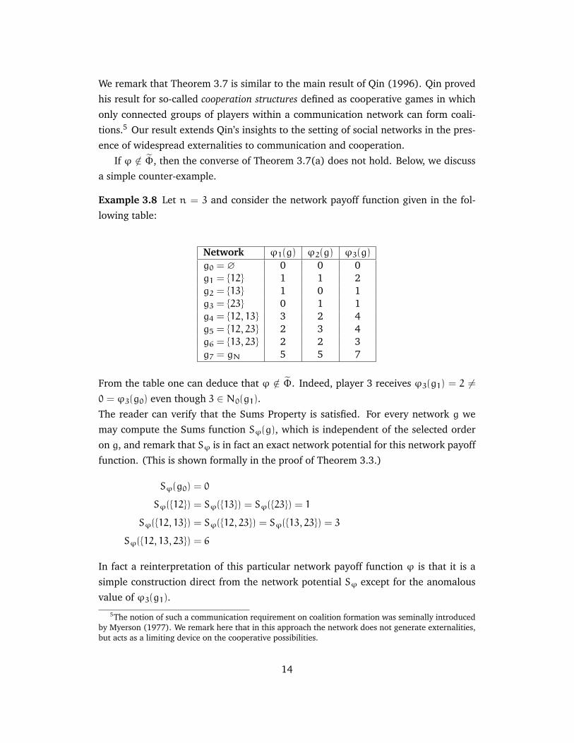
Example 3.8 Let n = 3 and consider the network payoff function given in the fol-

lowing table:

Network ϕ1(g) ϕ2(g) ϕ3(g)

g0 = ∅ 0 0 0g1 = {12} 1 1 2g2 = {13} 1 0 1g3 = {23} 0 1 1g4 = {12, 13} 3 2 4g5 = {12, 23} 2 3 4g6 = {13, 23} 2 2 3g7 = gN 5 5 7

From the table one can deduce that ϕ /∈ Φ. Indeed, player 3 receives ϕ3(g1) = 2 6=0 = ϕ3(g0) even though 3 ∈ N0(g1).The reader can verify that the Sums Property is satisfied. For every network g we

may compute the Sums function Sϕ(g), which is independent of the selected order

on g, and remark that Sϕ is in fact an exact network potential for this network payoff

function. (This is shown formally in the proof of Theorem 3.3.)

Sϕ(g0) = 0

Sϕ({12}) = Sϕ({13}) = Sϕ({23}) = 1

Sϕ({12, 13}) = Sϕ({12, 23}) = Sϕ({13, 23}) = 3

Sϕ({12, 13, 23}) = 6

In fact a reinterpretation of this particular network payoff function ϕ is that it is a

simple construction direct from the network potential Sϕ except for the anomalous

value of ϕ3(g1).

5The notion of such a communication requirement on coalition formation was seminally introducedby Myerson (1977). We remark here that in this approach the network does not generate externalities,but acts as a limiting device on the cooperative possibilities.

14

Now one can verify that for the network g1 the constructed cooperative game U =

Uϕ,g1is given by

U(∅) = U(1) = U(2) = U(3) = 0

U(12) = 2

U(13) = U(23) = 0

U(123) = 4

This cooperative game has a Shapley value given by φ(U) = (123 , 123 ,23) 6= (1, 1, 2) =

ϕ(g1). Thus, this payoff function—although admitting an exact network potential—

does not satisfy Shapley consistency. �

4 Ordinal Network Potentials

We proceed to discuss ordinal network potentials and explore their relationship with

ordinal potentials of the corresponding Consent Game. Ordinal network potentials

generalize the notion of an exact network potential from cardinal structures to or-

dinal structures similarly as seminally introduced by Monderer and Shapley (1996).

We subsequently examine the properties of network payoff functions admitting such

ordinal network potentials.

Like we did for the case of exact network potentials, we are only able to introduce

the notion of an ordinal network potential for a class of network payoff functions

that satisfies the so-called pairwise sign compatibility condition, which generalizes

the equal bargaining power requirement.

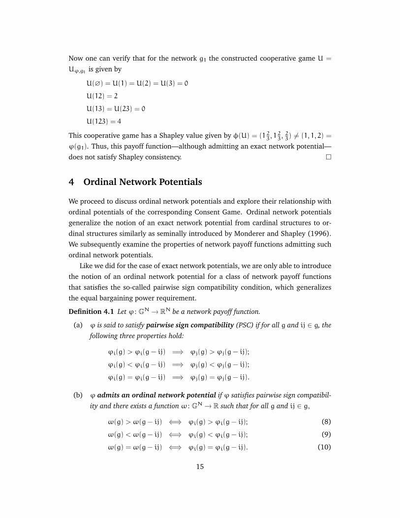
Definition 4.1 Let ϕ : GN → RN be a network payoff function.

(a) ϕ is said to satisfy pairwise sign compatibility (PSC) if for all g and ij ∈ g, thefollowing three properties hold:

ϕi(g) > ϕi(g− ij) =⇒ ϕj(g) > ϕj(g− ij);

ϕi(g) < ϕi(g− ij) =⇒ ϕj(g) < ϕj(g− ij);

ϕi(g) = ϕi(g− ij) =⇒ ϕj(g) = ϕj(g− ij).

(b) ϕ admits an ordinal network potential if ϕ satisfies pairwise sign compatibil-ity and there exists a function ω : GN → R such that for all g and ij ∈ g,

ω(g) > ω(g− ij) ⇐⇒ ϕi(g) > ϕi(g− ij); (8)

ω(g) < ω(g− ij) ⇐⇒ ϕi(g) < ϕi(g− ij); (9)

ω(g) = ω(g− ij) ⇐⇒ ϕi(g) = ϕi(g− ij). (10)

15

We introduce a short-hand notation for denoting the above, namely, (8), (9) and (10)

are equivalent to Sign (ω(g),ω(g− ij)) = Sign (ϕi(g), ϕi(g− ij)).

To illustrate the introduction of the concept of an ordinal network potential we

return to the case of link-based network payoffs already discussed in Example 3.4.

The following illustrates when ordinal network potentials can be admitted for that

particular case.

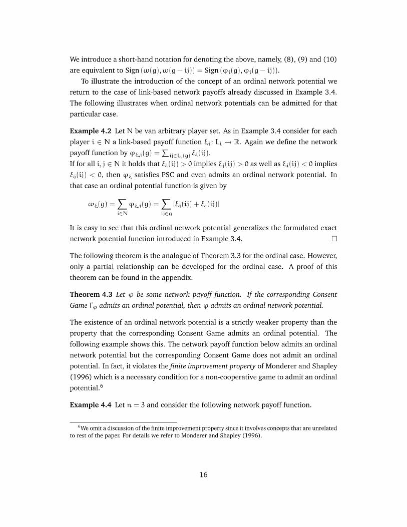
Example 4.2 Let N be van arbitrary player set. As in Example 3.4 consider for each

player i ∈ N a link-based payoff function ξi : Li → R. Again we define the network

payoff function by ϕξ,i(g) =∑ij∈Li(g)

ξi(ij).

If for all i, j ∈ N it holds that ξi(ij) > 0 implies ξj(ij) > 0 as well as ξi(ij) < 0 implies

ξj(ij) < 0, then ϕξ satisfies PSC and even admits an ordinal network potential. In

that case an ordinal potential function is given by

ωξ(g) =∑i∈N

ϕξ,i(g) =∑ij∈g

[ξi(ij) + ξj(ij)]

It is easy to see that this ordinal network potential generalizes the formulated exact

network potential function introduced in Example 3.4. �

The following theorem is the analogue of Theorem 3.3 for the ordinal case. However,

only a partial relationship can be developed for the ordinal case. A proof of this

theorem can be found in the appendix.

Theorem 4.3 Let ϕ be some network payoff function. If the corresponding ConsentGame Γϕ admits an ordinal potential, then ϕ admits an ordinal network potential.

The existence of an ordinal network potential is a strictly weaker property than the

property that the corresponding Consent Game admits an ordinal potential. The

following example shows this. The network payoff function below admits an ordinal

network potential but the corresponding Consent Game does not admit an ordinal

potential. In fact, it violates the finite improvement property of Monderer and Shapley

(1996) which is a necessary condition for a non-cooperative game to admit an ordinal

potential.6

Example 4.4 Let n = 3 and consider the following network payoff function.

6We omit a discussion of the finite improvement property since it involves concepts that are unrelatedto rest of the paper. For details we refer to Monderer and Shapley (1996).

16

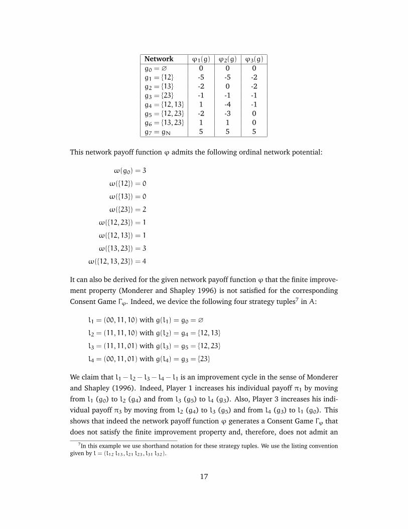
Network ϕ1(g) ϕ2(g) ϕ3(g)

g0 = ∅ 0 0 0g1 = {12} -5 -5 -2g2 = {13} -2 0 -2g3 = {23} -1 -1 -1g4 = {12, 13} 1 -4 -1g5 = {12, 23} -2 -3 0g6 = {13, 23} 1 1 0g7 = gN 5 5 5

This network payoff function ϕ admits the following ordinal network potential:

ω(g0) = 3

ω({12}) = 0

ω({13}) = 0

ω({23}) = 2

ω({12, 23}) = 1

ω({12, 13}) = 1

ω({13, 23}) = 3

ω({12, 13, 23}) = 4

It can also be derived for the given network payoff function ϕ that the finite improve-

ment property (Monderer and Shapley 1996) is not satisfied for the corresponding

Consent Game Γϕ. Indeed, we device the following four strategy tuples7 in A:

l1 = (00, 11, 10) with g(l1) = g0 = ∅

l2 = (11, 11, 10) with g(l2) = g4 = {12, 13}

l3 = (11, 11, 01) with g(l3) = g5 = {12, 23}

l4 = (00, 11, 01) with g(l4) = g3 = {23}

We claim that l1 − l2 − l3 − l4 − l1 is an improvement cycle in the sense of Monderer

and Shapley (1996). Indeed, Player 1 increases his individual payoff π1 by moving

from l1 (g0) to l2 (g4) and from l3 (g5) to l4 (g3). Also, Player 3 increases his indi-

vidual payoff π3 by moving from l2 (g4) to l3 (g5) and from l4 (g3) to l1 (g0). This

shows that indeed the network payoff function ϕ generates a Consent Game Γϕ that

does not satisfy the finite improvement property and, therefore, does not admit an

7In this example we use shorthand notation for these strategy tuples. We use the listing conventiongiven by l = (l12 l13, l21 l23, l31 l32).

17

ordinal potential.

The underlying motive is mainly that non-cooperative game theoretic improvement

paths are very different in nature from link-based improvement paths as introduced

in the next section. Indeed, individual players are completely in control of the strate-

gies that they select. This is fundamentally different from the coordinated strategic

modification underlying a link-based improvement. �

In the next section we discuss several properties of network payoff function which ad-

mit ordinal network potentials and those for which the corresponding Consent Game

admits an ordinal potential. We introduce the following three classes of network

payoff functions:

Φ1: This is the set of network payoff functions ϕ that admit an exact network po-

tential. This is equivalent to the requirement that the corresponding Consent

Game Γϕ admits an exact potential.

Φ2: This is the set of network payoff functions ϕ for which the corresponding Con-

sent Game Γϕ admits an ordinal potential.

Φ3: This is the set of network payoff functions ϕ that admit an ordinal network

potential.

From the above definitions, it can be concluded that

∅ 6= Φ1 Φ2 Φ3.

We emphasize that in principle there is no link of the sets introduced above with the

collection Φ introduced in the preceding section of this paper.

5 Potentials and network stability

In this section we discuss the relationship between the existence of an ordinal net-

work potential and the convergence of improvement paths to a pairwise stable net-

work in the sense of Jackson and Watts (2002a). Subsequently we consider simi-

lar questions with regard to network payoff functions in the class Φ2 for which the

corresponding Consent Game admits an ordinal potential. We show that these pay-

off functions imply stronger convergence and existence properties. (Jackson and

Watts 2001)

18

5.1 Improvement processes

We first introduce some concepts taken from Jackson and Watts (2002a) and Jackson

and Watts (2002b).8

Definition 5.1 An improvement path from a network g to a network g′ is a finitesequence of adjacent networks g1, g2, . . . , gK with g1 = g and gK = g′ such that for anyk ∈ {1, . . . , K− 1} either

(i) gk+1 = gk − ij for some ij such that ϕi(gk − ij) > ϕi(gk), or

(ii) gk+1 = gk + ij for some ij such that ϕi(gk + ij) > ϕi(gk) and ϕj(gk + ij) >

ϕj(gk).

An improvement path C ⊂ GN is an improvement cycle if for any g ∈ C and g′ ∈ Cthere exists an improvement path from g to g′.If there is an improvement path from g to g′ and g and g′ are adjacent, then we also saythat g′ defeats g. It should be clear that every pairwise stable network is undefeated.

It is obvious that if there are no improvement cycles, then the network payoff function

admits a pairwise stable network. This is because in general there are three possibil-

ities. First, there are no improvement paths, in which case every network is pairwise

stable. Second, every improvement path terminates in some pairwise stable network.

Third, there is at least one improvement path that does not terminate. Given that

there are only a finite number of networks, the latter simply means there exists an

improvement cycle. Therefore, the absence of improvement cycles guarantees exis-

tence of at least one pairwise stable network. We formalize this using the following

insight, which forms the foundation of the research on pairwise stable networks of

Jackson and Watts (2002a) and Jackson and Watts (2001).

Lemma 5.2 : Corollary to Jackson and Watts (2001, Lemma 1).

Given any network payoff function, there either exists at least one improvement cycle orat least one pairwise stable network.

In fact, Jackson and Watts (2001) prove a much stronger result, namely that there

exists at least one closed improvement cycle or at least one pairwise stable network,

a closed improvement cycle being an improvement cycle such that there are no al-

ternative improvement paths emanating from any of the networks that are part of8The terminology of an “improvement path” introduced here should be distinguished strictly from

the concept with the same name in non-cooperative game theory. The notion developed here refersto a sequence of networks with certain properties rather than a sequence of strategy tuples as used innon-cooperative game theory.

19

the improvement cycle. Jackson and Watts (2001) have also defined necessary and

sufficient conditions for absence of improvement cycles.

Next we turn to the discussion of the relationship between improvement paths

and the presence of ordinal network potentials.

Theorem 5.3 If ϕ ∈ Φ3 admits an ordinal network potential, then the following prop-erties hold:

(a) There exists at least one pairwise stable network;

(b) There are no improvement cycles;

(c) The set of strongly pairwise stable and strictly pairwise stable networks coincide.

For a proof of Theorem 5.3 we refer to the appendix.

The converse of assertion 5.3(b) is not true. There can be payoff functions without

improvement cycles, but for which there does not exist an ordinal network potential.

The next counter-example is a modification of an example developed in Jackson and

Watts (2001).

Example 5.4 Let n = 3. Suppose the network payoff function is such that {12, 23, 13}

defeats {12, 23} defeats {12} defeats {12, 13}, but that players 2 and 3 are both indif-

ferent between {12, 23, 13} and {12, 13}. Suppose also no other network defeats any

other. Here the reader can verify that there are no improvement cycles. But we can

show that no ordinal network potential exists.

Suppose by contradiction that an ordinal network potential, say ω, exists. Then, by

definition since {12, 23, 13} defeats {12, 23} defeats {12} defeats {12, 13}, it has to hold

that

ω({12, 23, 13}) > ω({12, 23})

ω({12, 23}) > ω({12})

ω({12}) > ω({12, 13})

Hence, ω({12, 23, 13}) > ω({12, 13}). But the fact that 2 and 3 are both indifferent

between {12, 23, 13} and {12, 13} implies

ω({12, 23, 13}) = ω({12, 13})

which is a contradiction. �

20

Next, we show that two additional conditions, Pairwise Sign Compatibility and a “no

indifference” condition guarantee the existence of ordinal network potential. In the

above case, no indifference is violated. The used terminology follows Jackson and

Watts (2001).

The network payoff function exhibits no indifference if for any two adjacent net-

works g and g′, either g defeats g′ or g′ defeats g.

We can now establish the sufficient conditions for existence of ordinal network

potentials. For a proof of the next theorem we refer as usual to the appendix.

Theorem 5.5 If the network payoff function satisfies Pairwise Sign Compatibility, ex-hibits no indifference, and is such that there are no improvement cycles, then the networkpayoff function admits an ordinal network potential and hence belongs to Φ3.

5.2 Existence of strictly pairwise stable networks

Next we address the implications of the existence of potentials for the existence of

pairwise stable networks. As Jackson and Watts (2001) show, improvement paths in

general converge to pairwise stable networks. Hence, if convergence can be estab-

lished, the existence of such networks is guaranteed as well. This is closely related to

the presence of potential functions as originally pointed out by Jackson and Watts.

Here we generalize the findings of Jackson and Watts. In particular, we are able to

show that for the subclass Φ2 of network payoff functions for which the correspond-

ing Consent Game has an ordinal potential, we can guarantee the existence of strictlypairwise stable networks. This rather strong existence result implies, therefore, the

existence of strongly pairwise stable as well as regular pairwise stable networks.

Theorem 5.6 If ϕ ∈ Φ2, then there exists at least one strictly pairwise stable network.

The proof of Theorem 5.6 is based on the fact that, given that there are a finite

number of strategy tuples in the corresponding Consent Game, for any ϕ ∈ Φ2 there

exists an ordinal potential maximizer. This potential maximizer corresponds to a

strictly pairwise stable network.

This raises the question whether every strictly or strongly pairwise stable net-

work is supported through a potential maximizer of the Consent game. The next

counterexample shows this is not the case.

Example 5.7 Let n = 3 and consider the network payoff function be given by

ϕk(g) = 1 for all k ∈ N if g = {ij, ih} has a line topology, and

ϕi(g) = 0 for all i ∈ N and for all other g ∈ GN.

21

This network payoff function admits an exact network potential, i.e., ϕ ∈ Φ1 and,

hence, ϕ ∈ Φ2.9 Now consider the empty network g0. It is strongly pairwise stable,

and, consequently, strictly pairwise stable as well. Indeed, there are no links to be

deleted and addition of any one link will not change payoffs.

Next, we show that a strategy tuple supporting g0 is not necessarily a potential max-

imizer. First, consider the strategy tuple l given by l = (00, 10, 10). It supports the

empty network. But it is not an ordinal potential maximizer. Let Q be an arbitrary

ordinal potential of the corresponding Consent Game (A,π). Then, define l1 ∈ A1 to

be such that l12 = l13 = 1, then

π1(l1, l−1) = 1 > 0 = π1(l) ⇒ Q(l1, l−1) > Q(l)

and hence l is not an ordinal potential maximizer. In fact, we can extend this reason-

ing and show that none of the strategy tuples supporting the empty network g0 are

ordinal potential maximizers. �

6 Some applications

In this section we discuss several applications of the theory of network potentials

developed in the previous sections. First we turn shortly to a well-known applica-

tion from social network theory, the so-called connections model, due to Jackson and

Wolinsky (1996).

Subsequently we turn to the discussion of the introduction of costs in the link for-

mation process. (Gilles, Chakrabarti, and Sarangi 2005a) If link formation is costly,

we show that essentially the main implication of the presence of network potentials is

not affected. Under both two-sided and one-sided link formation costs, the presence

of a network potential implies that the Consent Game admits a potential as well. It

should be clear that the reverse of this implication can no longer be guaranteed as is

the case for costless link formation.

6.1 The connections model

We illustrate Theorem 4.3 with an application that illustrates the applicability of ordi-

nal network potentials to models considered in the literature. The connections model

describes that communication over multiple links reduces the resulting benefits ex-

ponentially. Besides social applications, the connections model has application in

9In fact, an exact network potential function ω for ϕ is given by ω(g) = 1 for g = {ij, ik} with a linetopology and ω(g) = 0 for all other g ∈ GN.

22

engineering, in particular wireless mobile ad-hoc networks. (Srivastava, Neel, Hicks,

MacKenzie, Lau, DaSilva, Reed, and Gilles 2005)

Let the player set N be arbitrary and consider any g ∈ GN. The connections

network payoff function for player i in network g is now given by

ϕδi (g) =∑j6=iδtij(g) −

∑j : ij∈g

cij (11)

where 0 < δ < 1, cij > 0 is the cost of establishing link ij for player i, and tij(g) is

the number of links on the shortest path between i and j. The number tij(g) is also

called the “geodesic distance” between i and j in network g. (If i and j are not linked,

i.e., ij /∈ g, then tij(g) = ∞ by convention.) If for the connections model given in

(11) it holds that all link formation costs are equal, i.e., cij = c > 0, then we refer to

this setup as the symmetric connections model.

In the symmetric connections model, if c < δ − δ2, then ϕδ admits an ordinal

network potential. In that case, any link formed increases the payoffs of both players

forming the link and does not reduce the payoffs of all the other players. Hence, by

definition, ω(g) =∑i∈Nϕ

δi (g) is an ordinal network potential.

6.2 Two-sided link formation costs

Let N = {1, . . . , n} be a given set of players and ψ : GN → RN+ be a fixed, but arbitrary

network benefit function representing the gross benefits that accrue to the players in

a network.10 For every player i ∈ N we introduce individualized link formation costs

represented by ci = (cij)j6=i ∈ RN\{i}+ . (Note that for some links ij ∈ gN it might hold

that cij 6= cji.) Thus, the pair 〈ψ, c〉 represents the basic payoffs and costs of network

formation to the individuals in N.

As in the standard Consent Game we let for every player i ∈ N her action set be

given by

Ai = {(lij)j6=i | lij ∈ {0, 1} }

As before, player i seeks contact with player j if lij = 1 and a link is formed if both

players seek contact, i.e., lij = lji = 1.

Let A =∏i∈NAi where l ∈ A. Then the resulting network is given by

g(l) = {ij ∈ gN | lij = lji = 1}.

10We emphasize that a network benefit function is simply a network payoff function that only admitsnon-negative payoffs to the players.

23

Now, however, link formation is costly. Approaching player j to form a link costs

player i an amount cij > 0. This results in the following game theoretic payoff

function for player i:

πai (l) = ψi(ga(l)) −

∑j6=ilij · cij (12)

where c is the link formation cost introduced above.

The pair 〈ψ, c〉 thus generates the non-cooperative game Γ2(ψ, c) = (A,πa) as

described above. The game Γ2(ψ, c) is denoted as the Consent Game under two-sidedlink formation costs.

Proposition 6.1 Consider the Consent Game under two-sided link formation costs Γ2(ψ, c)based on 〈ψ, c〉. If ψ ∈ Φ1 is a network benefit function that admits an exact networkpotential, then the Consent Game under two-sided link formation costs admits an exactpotential.

Proof. Let ψ admit an exact potential ω : GN → R. Now consider the function

Qa : A → R given by

Qa(l) = ω(g(l)) −∑ij∈gN

[ lij · cij + lji · cji ]

Using similar arguments as used in the proof of theorem 3.3, we now can show that

the function Qa is in fact an exact potential for the Consent Game under two-sided

link formation costs (A,πa).

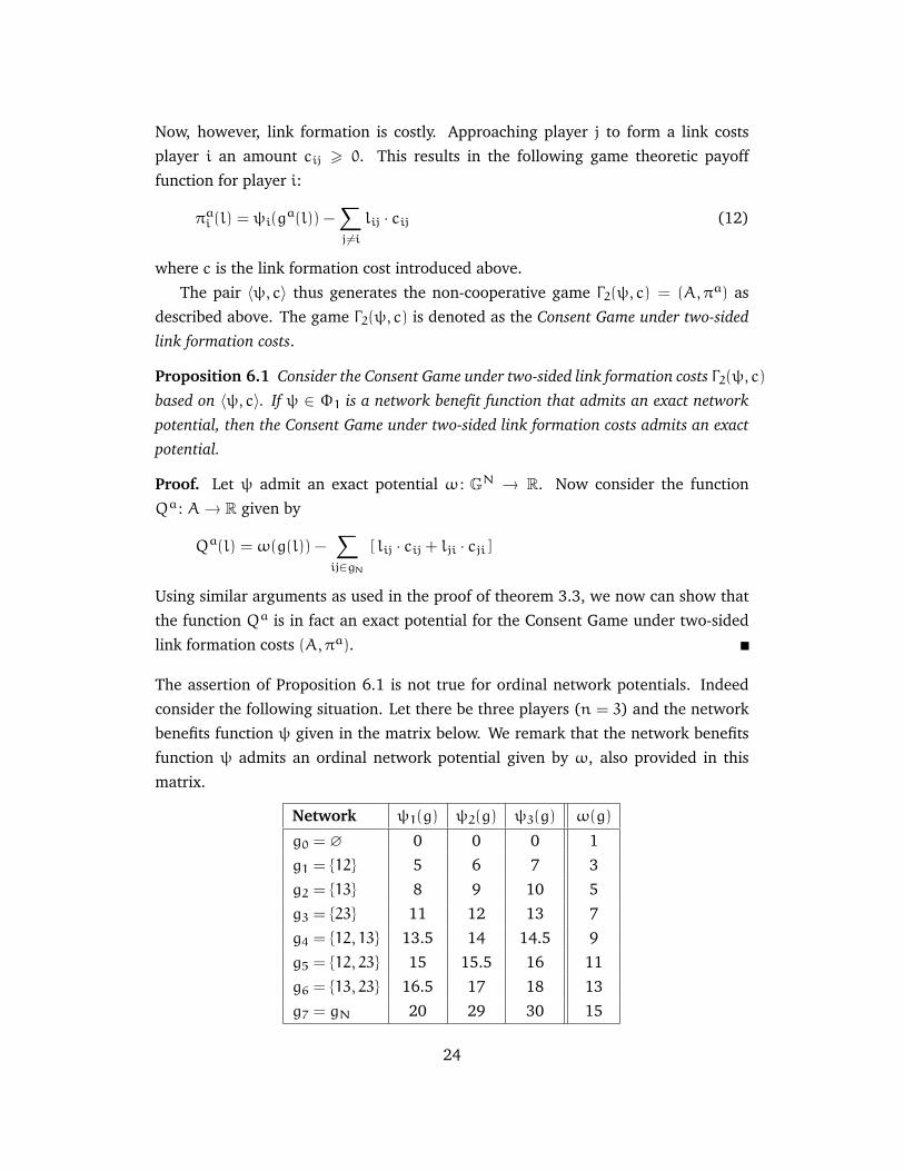
The assertion of Proposition 6.1 is not true for ordinal network potentials. Indeed

consider the following situation. Let there be three players (n = 3) and the network

benefits function ψ given in the matrix below. We remark that the network benefits

function ψ admits an ordinal network potential given by ω, also provided in this

matrix.

Network ψ1(g) ψ2(g) ψ3(g) ω(g)

g0 = ∅ 0 0 0 1

g1 = {12} 5 6 7 3

g2 = {13} 8 9 10 5

g3 = {23} 11 12 13 7

g4 = {12, 13} 13.5 14 14.5 9

g5 = {12, 23} 15 15.5 16 11

g6 = {13, 23} 16.5 17 18 13

g7 = gN 20 29 30 15

24

Next consider costly network formation such that c12 = 4, c31 = 6, c23 = 13, and

cij = 0 for all other ordered pairs ij /∈ {12, 31, 23}.

Within the provided setting we can now construct an improvement cycle in the

consent game under two-sided link formation costs Γ2(ψ, c), thus showing that the

impossibility that this game admits an ordinal potential. This improvement cycle is

as follows:

l1 = (11, 11, 11) with g(l1) = g7 = gN

l2 = (01, 11, 11) with g(l2) = g5

l3 = (01, 11, 01) with g(l3) = g3

l4 = (01, 10, 01) with g(l4) = g0 = ∅

l5 = (11, 10, 01) with g(l5) = g1

l6 = (11, 10, 11) with g(l6) = g4

It is easy to see that this strategy sequence indeed constitutes an improvement cycle

in Γ2(ψ, c).

This shows the claim that even though the network benefit function ψ admits an

ordinal potential, the resulting consent game under two-sided link formation costs

does not necessarily have to admit an ordinal potential.

6.3 One-sided link formation costs

In this section we discuss the Consent Game under one-sided link formation costs.

Here links are formed by mutual agreement, but only one player in the pair under

consideration initiates the link formation process and the other player only responds

to this link formation attempt. The initiator incurs the formation costs of the link,

while the respondent incurs no costs. Our discussion follows the setup developed in

Gilles, Chakrabarti, and Sarangi (2005a).11 Hence, a different strategy space reflect-

ing the difference between initiator and respondent is called for.

Formally, consider an arbitrary player set N and a non-negative network benefit

function ψ : GN → RN+ . To model the separation of the initiation of links and the re-

sponding to link formation initiations, we introduce for every player i ∈ N a strategy

set given by

Abi = {(lij, rij)j6=i | lij, rij ∈ {0, 1} }. (13)

11We remark that a similar link formation structure has been already discussed by Slikker (2000) andSlikker, Gilles, Norde, and Tijs (2005) in the context of the formation of directed networks. See alsoDutta and Jackson (2000).

25

Player i acts as the initiator in forming a link with player j if lij = 1. Player j responds

positively to this initiative if rji = 1. A link is established if formation is initiated and

accepted, i.e., if lij = rji = 1. This is formalized as follows.

Let Ab =∏i∈NA

bi be the corresponding strategy tuple space. Given the link

formation procedure described, for any (l, r) ∈ Ab, the resulting network is now

given by

gb(l, r) = {ij ∈ gN | lij = rji = 1}. (14)

When player i initiates the formation of a link with player j she incurs a cost of

cij > 0. Responding to the initiative by another player, however, is costless. This

results in the following game theoretic payoff function for player i:

πbi (l, r) = ϕi(gb(l, r)) −

∑j6=ilij · cij (15)

where c denotes the link formation costs.

Analogous to the previous model with two-sided link formation costs, the pair

〈ψ, c〉 now generates the non-cooperative game Γ1(ψ, c) = (Ab, πb) introduced above.

The game Γ1(ψ, c) represents the Consent Game under one-sided link formation costs.The next proposition shows only a partial statement of the similar proposition

formulated for the Consent Game under two-sided link formation costs. The structure

of one-sided link formation costs is based on a fundamental asymmetry that can no

longer be linked directly to standard Consent Game Γψ based on the benefit function

ψ admitting an ordinal potential.

Proposition 6.2 Let Γ1(ψ, c) be the Consent Game under one-sided link formation costsbased on 〈ψ, c〉. If ψ ∈ Φ1 admits an exact network potential, then the Consent Gameunder one-sided link formation costs Γ1(ψ, c) admits an exact potential.

Proof. Let ψ ∈ Φ1 admit an exact potential ω : GN → R. Now consider the function

Qb : Ab → R given by

Qb(l, r) = ω(gb(l, r)) −∑ij∈gN

[ lij · cij + lji · cji ]

Again using similar techniques as used in the proof of Theorem 3.3 we can now

show that the function Qb is in fact an exact potential for the Consent Game under

one-sided link formation costs Γ1(ψ, c).

26

7 Coda

While potentials are defined for non-cooperative games, a similar notion called net-

work potentials can be defined for network payoff functions. It is closely related

to the potentials of a non-cooperative link formation game due to Myerson (1991).

An exact network potential exists if and only if the Consent Game admits an exact

potential. The existence of network ordinal potentials is however weaker than the

existence of ordinal potentials for the Consent Game. When these potentials exist,

the network payoff function has attractive properties. When exact network potentials

exist, there exists both a strongly pairwise stable and a strictly pairwise stable net-

work. Under the much weaker condition of the existence of ordinal potentials, there

are no network improvement cycles, at least one pairwise stable network exists and

the set of strongly pairwise stable and strictly pairwise stable networks coincide.

Topics for further research include when does existence of ordinal network po-

tentials guarantee that the Consent Game has an ordinal potential. Another topic

of interest is what are the interesting examples of network payoff functions satisfy

the somewhat demanding conditions of the existence of exact and ordinal network

payoff functions. Gilles, Chakrabarti, and Sarangi (2005b) discuss an example of

network payoff function for which an exact network potential exists.

27

References

BALA, V., AND S. GOYAL (2000): “A Non-Cooperative Model of Network Formation,”Econometrica, 68, 1181–1230.

BARON, R., J. DURIEU, H. HALLER, AND P. SOLAL (2006): “Complexity and StochasticEvolution of Dyadic Networks,” Computers & Operations Research, 33, 312–327.

BLOCH, F., AND M. O. JACKSON (2004): “The Formation of Networks with Transfersamong Players,” Working Paper, GREQAM, Universite d’Aix-Marseille, Marseille,France.

DUTTA, B., AND M. O. JACKSON (2000): “The Stability and Efficiency of DirectedCommunication Networks,” Review of Economic Design, 5, 251–272.

DUTTA, B., A. VAN DEN NOUWELAND, AND S. TIJS (1998): “Link Formation in Coop-erative Situations,” International Journal of Game Theory, 27, 245–256.

GILLES, R. P., S. CHAKRABARTI, AND S. SARANGI (2005a): “Social Network Forma-tion with Consent: Nash Equilibria and Pairwise Refinements,” Working paper,Department of Economics, Virginia Tech, Blacksburg, VA.

(2005b): “Stability and Link-Based Network Payoffs,” Working paper, De-partment of Economics, Virginia Tech, Blacksburg, VA.

GILLES, R. P., S. CHAKRABARTI, S. SARANGI, AND N. BADASYAN (2005): “NetworkIntermediaries,” Working Paper, Department of Economics, Virginia Tech, Blacks-burg, Virginia.

GILLES, R. P., AND S. SARANGI (2005a): “Building Social Networks,” Working Paper,Department of Economics, Virginia Tech, Blacksburg, VA.

(2005b): “Stable Networks and Convex Payoffs,” CentER Discussion Paper2005-84, Tilburg University, Tilburg, the Netherlands.

HART, S., AND A. MAS-COLELL (1989): “Potential, Value, and Consistency,” Econo-metrica, 57, 589–614.

JACKSON, M. O. (2003): “the Stability and efficiency of economic and Social Net-works,” in Networks and Groups: Models of Strategic Formation, ed. by B. Dutta,and M. O. Jackson, pp. 97–140. Springer Verlag, New York, NY.

(2005a): “Allocation Rules for Network Games,” Games and Economic Behav-ior, 51, 128–154.

(2005b): “A Survey of Models of Network Formation: Stability and Effi-ciency,” in Group Formation in Economics: Networks, Clubs, and Coalitions, ed. byG. Demange, and M. Wooders, chap. 1, pp. 11–57. Cambridge University Press,Cambridge, United Kingdom.

28

JACKSON, M. O., AND A. WATTS (2001): “The Existence of Pairwise Stable Networks,”Seoul Journal of Economics, 14(3), 299–321.

(2002a): “The Evolution of Social and Economic Networks,” Journal of Eco-nomic Theory, 106, 265–295.

(2002b): “On the Formation of Interaction Networks in Social CoordinationGames,” Games and Economic Behavior, 41, 265–291.

JACKSON, M. O., AND A. WOLINSKY (1996): “A Strategic Model of Social and Eco-nomic Networks,” Journal of Economic Theory, 71, 44–74.

MONDERER, D., AND L. S. SHAPLEY (1996): “Potential Games,” Games and EconomicBehavior, 14, 124–143.

MYERSON, R. B. (1977): “Graphs and Cooperation in Games,” Mathematics of Oper-ations Research, 2, 225–229.

(1991): Game Theory: Analysis of Conflict. Harvard University Press, Cam-bridge, MA.

QIN, C.-Z. (1996): “Endogenous Formation of Cooperation Structures,” Journal ofEconomic Theory, 69, 218–226.

ROSENTHAL, R. W. (1973): “A Class of Games Possessing Pure-Strategy Nash Equi-libria,” International Journal of Game Theory, 2, 65–67.

SHAPLEY, L. (1953): “A Value for n-Person Games,” in Contributiuons to the Theory ofGames, ed. by R. Luce, and A. Tucker, vol. II. Princeton University Press, Princeton,NJ.

(1971): “Cores of Convex Games,” International Journal of Game Theory, 1,11–26.

SLIKKER, M. (2000): “Decision Making and Cooperation Structures,” Ph.D. thesis,Tilburg University, Tilburg, The Netherlands.

SLIKKER, M., R. P. GILLES, H. NORDE, AND S. TIJS (2005): “Directed Networks,Payoff Properties, and Hierarchy Formation,” Mathematical Social Sciences, 49,55–80, in press.

SRIVASTAVA, V., J. NEEL, J. HICKS, A. MACKENZIE, K. LAU, L. DASILVA, J. REED,AND R. GILLES (2005): “Application of Game Theory to Distributed MANET Algo-rithms,” IEEE Communications Surveys and Tutorials, forthcoming.

UI, T. (2000): “A Shapley Value Representation of Potential Games,” Games andEconomic Behavior, 31, 121–135.

VOORNEVELD, M., AND H. NORDE (1997): “A Characterization of Ordinal PotentialGames,” Games and Economic Behavior, 19, 235–242.

29

Appendix: Proofs of the main results

Proof of Theorem 3.3

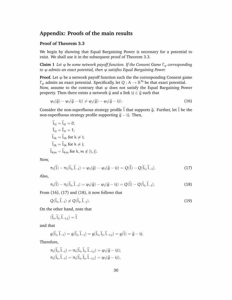
We begin by showing that Equal Bargaining Power is necessary for a potential toexist. We shall use it in the subsequent proof of Theorem 3.3.

Claim 1 Let ϕ be some network payoff function. If the Consent Game Γϕ correspondingto ϕ admits an exact potential, then ϕ satisfies Equal Bargaining Power.

Proof. Let ϕ be a network payoff function such the the corresponding Consent gameΓϕ admits an exact potential. Specifically, let Q : A → RN be that exact potential.Now, assume to the contrary that ϕ does not satisfy the Equal Bargaining Powerproperty. Then there exists a network g and a link ij ∈ g such that

ϕi(g) −ϕi(g− ij) 6= ϕj(g) −ϕj(g− ij). (16)

Consider the non-superfluous strategy profile l that supports g. Further, let l be thenon-superfluous strategy profile supporting g− ij. Then,

lij = lji = 0;

lij = lji = 1;

lik = lik for k 6= i;

ljk = ljk for k 6= j;

lkm = lkm for k,m /∈ {i, j}.

Now,

πi(l) − πi(li, l−i) = ϕi(g) −ϕi(g− ij) = Q(l) −Q(li, l−i). (17)

Also,

πj(l) − πj(lj, l−j) = ϕj(g) −ϕj(g− ij) = Q(l) −Q(lj, l−j). (18)

From (16), (17) and (18), it now follows that

Q(li, l−i) 6= Q(lj, l−j). (19)

On the other hand, note that

(li, lj, l−i,j) = l

and that

g(li, l−i) = g(lj, l−j) = g(li, lj, l−i,j) = g(l) = g− ij.

Therefore,

πi(lj, l−j) = πi(li, lj, l−i,j) = ϕi(g− ij);

πj(li, l−i) = πj(li, lj, l−i,j) = ϕj(g− ij),

30

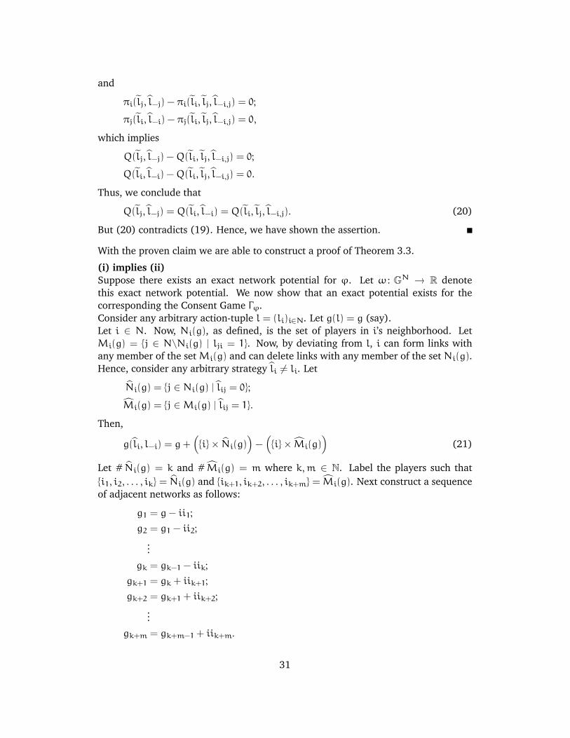
and

πi(lj, l−j) − πi(li, lj, l−i,j) = 0;

πj(li, l−i) − πj(li, lj, l−i,j) = 0,

which implies

Q(lj, l−j) −Q(li, lj, l−i,j) = 0;

Q(li, l−i) −Q(li, lj, l−i,j) = 0.

Thus, we conclude that

Q(lj, l−j) = Q(li, l−i) = Q(li, lj, l−i,j). (20)

But (20) contradicts (19). Hence, we have shown the assertion.

With the proven claim we are able to construct a proof of Theorem 3.3.

(i) implies (ii)Suppose there exists an exact network potential for ϕ. Let ω : GN → R denotethis exact network potential. We now show that an exact potential exists for thecorresponding the Consent Game Γϕ.Consider any arbitrary action-tuple l = (li)i∈N. Let g(l) = g (say).Let i ∈ N. Now, Ni(g), as defined, is the set of players in i’s neighborhood. LetMi(g) = {j ∈ N\Ni(g) | lji = 1}. Now, by deviating from l, i can form links withany member of the set Mi(g) and can delete links with any member of the set Ni(g).Hence, consider any arbitrary strategy li 6= li. Let

Ni(g) = {j ∈ Ni(g) | lij = 0};

Mi(g) = {j ∈Mi(g) | lij = 1}.

Then,

g(li, l−i) = g+({i}× Ni(g)

)−

({i}× Mi(g)

)(21)

Let # Ni(g) = k and # Mi(g) = m where k,m ∈ N. Label the players such that{i1, i2, . . . , ik} = Ni(g) and {ik+1, ik+2, . . . , ik+m} = Mi(g). Next construct a sequenceof adjacent networks as follows:

g1 = g− ii1;

g2 = g1 − ii2;

...

gk = gk−1 − iik;

gk+1 = gk + iik+1;

gk+2 = gk+1 + iik+2;

...

gk+m = gk+m−1 + iik+m.

31

From (21), it then follows that

gk+m = g(li, l−i). (22)

Now, from (6), it follows that

ω(g) −ω(g1) = ϕi(g) −ϕi(g1);

ω(g1) −ω(g2) = ϕi(g1) −ϕi(g2);

...

ω(gk−1) −ω(gk) = ϕi(gk−1) −ϕi(gk).

Adding both sides of all the expressions (which results in common terms cancellingout), we get

ω(g) −ω(gk) = ϕi(g) −ϕi(gk). (23)

Similarly, from (6), it follows that

ω(gk+m) −ω(gk) = ϕi(gk+m) −ϕi(gk). (24)

Taking the difference of (23) and (24), we get

ω(gk+m) −ω(g) = ϕi(gk+m) −ϕi(g). (25)

From (22) and (25), it follows

ω(g(li, l−i)) −ω(g(l)) = ϕi(g(li, l−i)) −ϕi(g(l)) = πi(li, l−i) − πi(l). (26)

Define a function Q : A → RN such that Q(l) = ω(g(l)). From (26), it now followsthat

Q(li, l−i) −Q(l) = πi(li, l−i) − πi(l).

This shows that, by definition, Q is indeed an exact potential of the correspondingConsent Game Γϕ.

(ii) implies (i)Suppose the Consent Game Γϕ admits an exact potential and that this potential isgiven by Q : A → R. We will show that ϕ now admits an exact network potential.We know from Claim 1 that Equal Bargaining Power must be satisfied. Hence, for allij ∈ g, g ∈ GN,

ϕi(g) −ϕi(g− ij) = ϕj(g) −ϕj(g− ij). (27)

Define ω : GN → R such that

ω(g) = Q(lg) (28)

32

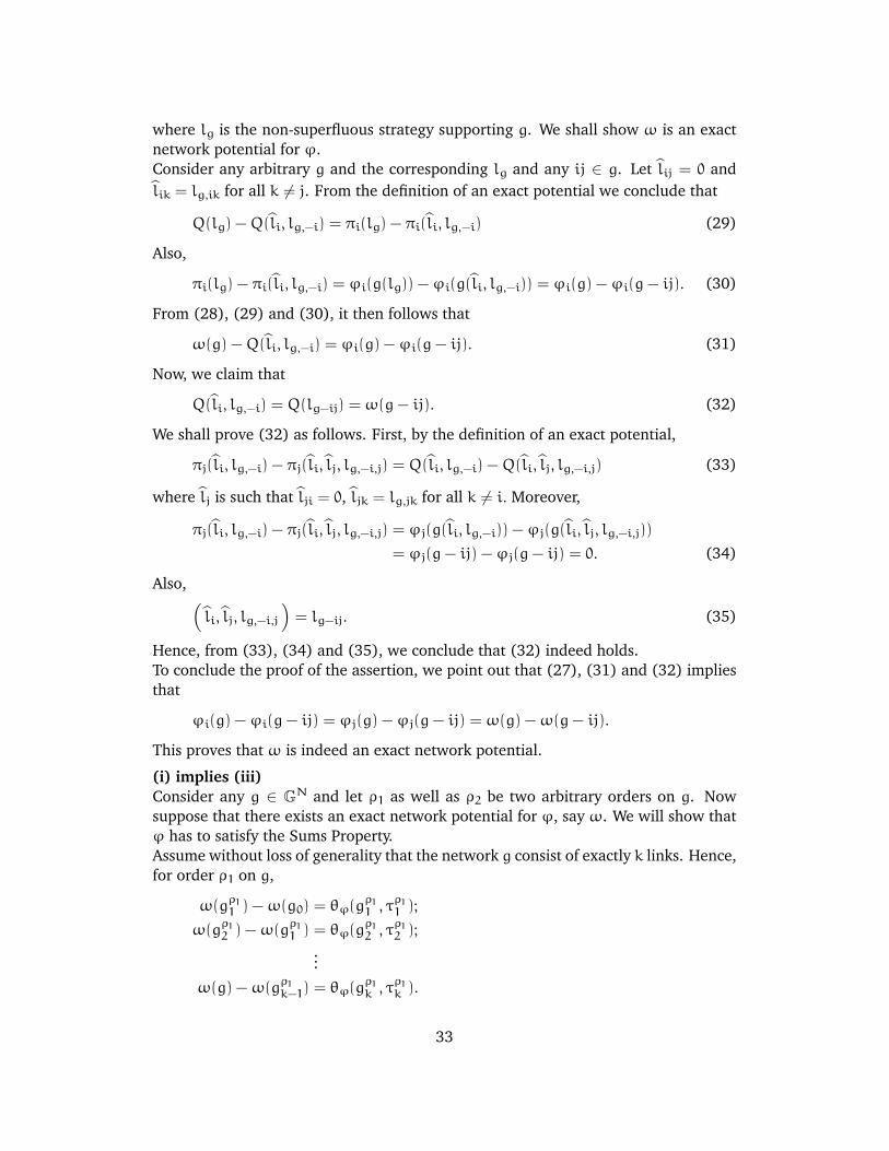
where lg is the non-superfluous strategy supporting g. We shall show ω is an exactnetwork potential for ϕ.Consider any arbitrary g and the corresponding lg and any ij ∈ g. Let lij = 0 andlik = lg,ik for all k 6= j. From the definition of an exact potential we conclude that

Q(lg) −Q(li, lg,−i) = πi(lg) − πi(li, lg,−i) (29)

Also,

πi(lg) − πi(li, lg,−i) = ϕi(g(lg)) −ϕi(g(li, lg,−i)) = ϕi(g) −ϕi(g− ij). (30)

From (28), (29) and (30), it then follows that

ω(g) −Q(li, lg,−i) = ϕi(g) −ϕi(g− ij). (31)

Now, we claim that

Q(li, lg,−i) = Q(lg−ij) = ω(g− ij). (32)

We shall prove (32) as follows. First, by the definition of an exact potential,

πj(li, lg,−i) − πj(li, lj, lg,−i,j) = Q(li, lg,−i) −Q(li, lj, lg,−i,j) (33)

where lj is such that lji = 0, ljk = lg,jk for all k 6= i. Moreover,

πj(li, lg,−i) − πj(li, lj, lg,−i,j) = ϕj(g(li, lg,−i)) −ϕj(g(li, lj, lg,−i,j))

= ϕj(g− ij) −ϕj(g− ij) = 0. (34)

Also, (li, lj, lg,−i,j

)= lg−ij. (35)

Hence, from (33), (34) and (35), we conclude that (32) indeed holds.To conclude the proof of the assertion, we point out that (27), (31) and (32) impliesthat

ϕi(g) −ϕi(g− ij) = ϕj(g) −ϕj(g− ij) = ω(g) −ω(g− ij).

This proves that ω is indeed an exact network potential.

(i) implies (iii)Consider any g ∈ GN and let ρ1 as well as ρ2 be two arbitrary orders on g. Nowsuppose that there exists an exact network potential for ϕ, say ω. We will show thatϕ has to satisfy the Sums Property.Assume without loss of generality that the network g consist of exactly k links. Hence,for order ρ1 on g,

ω(gρ11 ) −ω(g0) = θϕ(g

ρ11 , τ

ρ11 );

ω(gρ12 ) −ω(g

ρ11 ) = θϕ(g

ρ12 , τ

ρ12 );

...

ω(g) −ω(gρ1k−1) = θϕ(g

ρ1k , τ

ρ1k ).

33

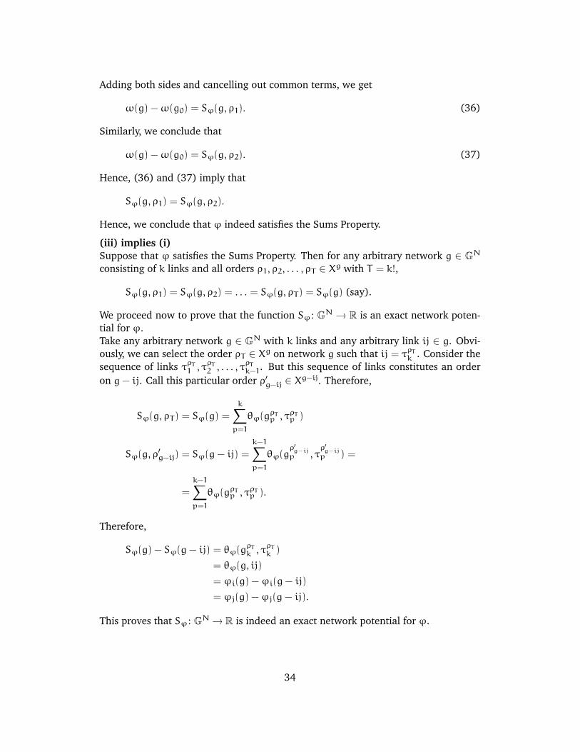
Adding both sides and cancelling out common terms, we get

ω(g) −ω(g0) = Sϕ(g, ρ1). (36)

Similarly, we conclude that

ω(g) −ω(g0) = Sϕ(g, ρ2). (37)

Hence, (36) and (37) imply that

Sϕ(g, ρ1) = Sϕ(g, ρ2).

Hence, we conclude that ϕ indeed satisfies the Sums Property.

(iii) implies (i)Suppose that ϕ satisfies the Sums Property. Then for any arbitrary network g ∈ GNconsisting of k links and all orders ρ1, ρ2, . . . , ρT ∈ Xg with T = k!,

Sϕ(g, ρ1) = Sϕ(g, ρ2) = . . . = Sϕ(g, ρT ) = Sϕ(g) (say).

We proceed now to prove that the function Sϕ : GN → R is an exact network poten-tial for ϕ.Take any arbitrary network g ∈ GN with k links and any arbitrary link ij ∈ g. Obvi-ously, we can select the order ρT ∈ Xg on network g such that ij = τ

ρTk . Consider the

sequence of links τρT1 , τ

ρT2 , . . . , τ

ρTk−1. But this sequence of links constitutes an order

on g− ij. Call this particular order ρ′g−ij ∈ Xg−ij. Therefore,

Sϕ(g, ρT ) = Sϕ(g) =

k∑p=1

θϕ(gρTp , τ

ρTp )

Sϕ(g, ρ′g−ij) = Sϕ(g− ij) =

k−1∑p=1

θϕ(gρ′g−ijp , τ

ρ′g−ijp ) =

=

k−1∑p=1

θϕ(gρTp , τ

ρTp ).

Therefore,

Sϕ(g) − Sϕ(g− ij) = θϕ(gρTk , τ

ρTk )

= θϕ(g, ij)

= ϕi(g) −ϕi(g− ij)

= ϕj(g) −ϕj(g− ij).

This proves that Sϕ : GN → R is indeed an exact network potential for ϕ.

34

Proof of Theorem 3.7

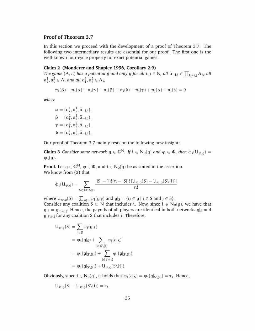
In this section we proceed with the development of a proof of Theorem 3.7. Thefollowing two intermediary results are essential for our proof. The first one is thewell-known four-cycle property for exact potential games.

Claim 2 (Monderer and Shapley 1996, Corollary 2.9)The game (A,π) has a potential if and only if for all i, j ∈ N, all a−i,j ∈

∏k6=i,jAk, all

a1i , a2i ∈ Ai and all a1j , a

2j ∈ Aj,

πi(β) − πi(α) + πj(γ) − πj(β) + πi(δ) − πi(γ) + πj(α) − πj(δ) = 0

where

α = (a1i , a1j , a−i,j),

β = (a2i , a1j , a−i,j),

γ = (a2i , a2j , a−i,j),

δ = (a1i , a2j , a−i,j).

Our proof of Theorem 3.7 mainly rests on the following new insight:

Claim 3 Consider some network g ∈ GN. If i ∈ N0(g) and ϕ ∈ Φ, then φi(Uϕ,g) =

ϕi(g).

Proof. Let g ∈ GN, ϕ ∈ Φ, and i ∈ N0(g) be as stated in the assertion.We know from (3) that

φi(Uϕ,g) =∑

S⊂N : S3i

(|S| − 1)!(n− |S|)! [Uϕ,g(S) −Uϕ,g(S\{i})]

n!

where Uϕ,g(S) =∑i∈Sϕi(g|S) and g|S = {ij ∈ g | i ∈ S and j ∈ S}.

Consider any coalition S ⊂ N that includes i. Now, since i ∈ N0(g), we have thatg|S = g|S\{i}. Hence, the payoffs of all players are identical in both networks g|S andg|S\{i} for any coalition S that includes i. Therefore,

Uϕ,g(S) =∑j∈Sϕj(g|S)

= ϕi(g|S) +∑j∈S\{i}

ϕj(g|S)

= ϕi(g|S\{i}) +∑j∈S\{i}

ϕj(g|S\{i})

= ϕi(g|S\{i}) +Uϕ,g(S\{i}).

Obviously, since i ∈ N0(g), it holds that ϕi(g|S) = ϕi(g|S\{i}) = τi. Hence,

Uϕ,g(S) −Uϕ,g(S\{i}) = τi.

35

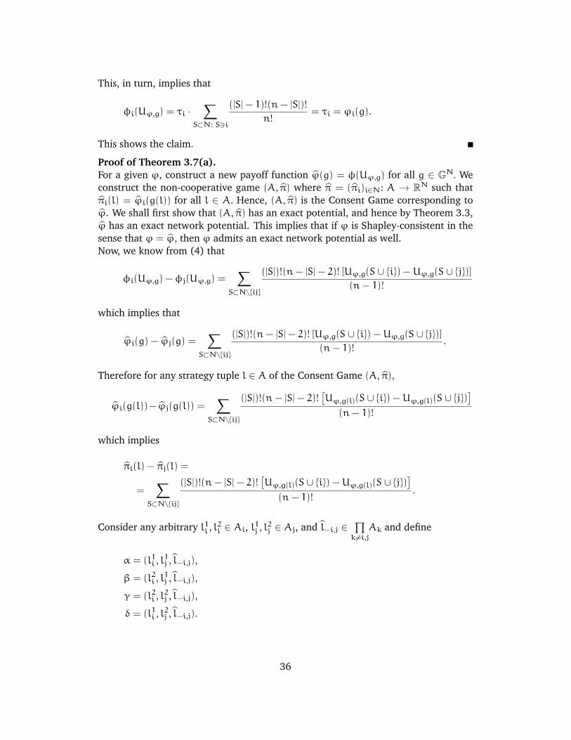
This, in turn, implies that

φi(Uϕ,g) = τi ·∑

S⊂N : S3i

(|S| − 1)!(n− |S|)!

n!= τi = ϕi(g).

This shows the claim.

Proof of Theorem 3.7(a).For a given ϕ, construct a new payoff function ϕ(g) = φ(Uϕ,g) for all g ∈ GN. Weconstruct the non-cooperative game (A, π) where π = (πi)i∈N : A → RN such thatπi(l) = ϕi(g(l)) for all l ∈ A. Hence, (A, π) is the Consent Game corresponding toϕ. We shall first show that (A, π) has an exact potential, and hence by Theorem 3.3,ϕ has an exact network potential. This implies that if ϕ is Shapley-consistent in thesense that ϕ = ϕ, then ϕ admits an exact network potential as well.Now, we know from (4) that

φi(Uϕ,g) −φj(Uϕ,g) =∑

S⊂N\{ij}

(|S|)!(n− |S| − 2)! [Uϕ,g(S ∪ {i}) −Uϕ,g(S ∪ {j})]

(n− 1)!

which implies that

ϕi(g) − ϕj(g) =∑

S⊂N\{ij}

(|S|)!(n− |S| − 2)! [Uϕ,g(S ∪ {i}) −Uϕ,g(S ∪ {j})]

(n− 1)!.

Therefore for any strategy tuple l ∈ A of the Consent Game (A, π),

ϕi(g(l))− ϕj(g(l)) =∑

S⊂N\{ij}

(|S|)!(n− |S| − 2)![Uϕ,g(l)(S ∪ {i}) −Uϕ,g(l)(S ∪ {j})

](n− 1)!

which implies

πi(l) − πj(l) =

=∑

S⊂N\{ij}

(|S|)!(n− |S| − 2)![Uϕ,g(l)(S ∪ {i}) −Uϕ,g(l)(S ∪ {j})

](n− 1)!

.

Consider any arbitrary l1i , l2i ∈ Ai, l1j , l2j ∈ Aj, and l−i,j ∈

∏k6=i,j

Ak and define

α = (l1i , l1j , l−i,j),

β = (l2i , l1j , l−i,j),

γ = (l2i , l2j , l−i,j),

δ = (l1i , l2j , l−i,j).

36

Then,

πi(β) − πi(α) + πj(γ) − πj(β) + πi(δ) − πi(γ) + πj(α) − πj(δ) =

= [πj(α) − πi(α)] + [πi(β) − πj(β)] + [πj(γ) − πi(γ)] + [πi(δ) − πj(δ)]

=∑

S⊂N\{ij}

(|S|)!(n− |S| − 2)!

(n− 1)!

[Uϕ,g(α)(S ∪ {j}) −Uϕ,g(α)(S ∪ {i})

]+

∑S⊂N\{ij}

(|S|)!(n− |S| − 2)!

(n− 1)!

[Uϕ,g(β)(S ∪ {i}) −Uϕ,g(β)(S ∪ {j})

]+

∑S⊂N\{ij}

(|S|)!(n− |S| − 2)!

(n− 1)!

[Uϕ,g(γ)(S ∪ {j}) −Uϕ,g(γ)(S ∪ {i})

]+

∑S⊂N\{ij}

(|S|)!(n− |S| − 2)!

(n− 1)!

[Uϕ,g(δ)(S ∪ {i}) −Uϕ,g(δ)(S ∪ {j})

]=

∑S⊂N\{ij}

(|S|)!(n− |S| − 2)!

(n− 1)!

[Uϕ,g(α)(S ∪ {j}) −Uϕ,g(β)(S ∪ {j})

]+

∑S⊂N\{ij}

(|S|)!(n− |S| − 2)!

(n− 1)!

[Uϕ,g(β)(S ∪ {i}) −Uϕ,g(γ)(S ∪ {i})

]+

∑S⊂N\{ij}

(|S|)!(n− |S| − 2)!

(n− 1)!

[Uϕ,g(γ)(S ∪ {j}) −Uϕ,g(δ)(S ∪ {j})

]+

∑S⊂N\{ij}

(|S|)!(n− |S| − 2)!

(n− 1)!

[Uϕ,g(δ)(S ∪ {i}) −Uϕ,g(α)(S ∪ {i})

].

Now, we claim that each of the four expressions in square brackets are zero. Startwith the first expression Uϕ,g(α)(S ∪ {j}) −Uϕ,g(β)(S ∪ {j}) for any S ⊂ N\{ij}. α andβ only differ in that player i changes her strategy from l1i in α to l2i in β. All otherplayers keep their strategies unchanged. But from the definition, both Uϕ,g(α)(S∪ {j})

and Uϕ,g(β)(S∪ {j}) are independent of strategies chosen by i. Therefore, Uϕ,g(α)(S∪{j}) −Uϕ,g(β)(S ∪ {j}) = 0. The same holds for the three other bracketed expressionsas well. Hence, by Claim 2, (A, π) admits an exact potential.

Proof of Theorem 3.7(b).Let the network payoff function ϕ admit an exact network potential. This impliesby Theorem 3.3 that the corresponding Consent Game Γϕ admits an exact potential.Let the potential function of the Consent Game corresponding to ϕ be denoted byP. Suppose to the contrary that the assertion does not hold and assume that ϕ(g) 6=φ(Uϕ,g) for some g ∈ GN.Now, we know from the earlier proof that if the payoff function were ϕ where ϕ(g) =

φ(Uϕ,g) for all g ∈ GN, then also the corresponding Consent Game has an exactpotential. Let the potential function of the Consent Game corresponding to ϕ bedenoted by P.

Claim: There exists a constant C ∈ R such that P(l) = P(l) + C for all l ∈ A.

37

We prove the claim by induction. Let for any i ∈ N, li ∈ Ai, ξ(li) = #{j ∈ N | lij = 1}.

Define an order ≺ on A such that l ≺ l′ if and only if there exists i ∈ N such thatξ(li) < ξ(l′i) and for all j < i, j ∈ N, ξ(lj) = ξ(l′j). Then, the smallest elementof A with respect to ≺ is given by l0 where l0ij = 0 for all i, j ∈ N, i 6= j. Set

C = P(l0) − P(l0). We shall show that if for all l ≺ l′, it holds that P(l) = P(l) + C,

then it is the case that P(l′) = P(l′) + C.For every i ∈ N, define li ∈ A as liij = 0 for all j 6= i and lijk = ljk for all j 6= i, k ∈ N.Then, li ≺ l and i ∈ N0(g(li)).Also, by definition of an exact potential, it must be the case that

πi(l) − πi(li) = P(l) − P(li)

=⇒ ϕi(g(l)) −ϕi(g(li)) = P(l) − P(li)

=⇒ ∑i∈Nϕi(g(l)) −

∑i∈Nϕi(g(l

i)) = n · P(l) −∑i∈NP(li)

=⇒ P(l) =

∑i∈Nϕi(g(l)) −

∑i∈Nϕi(g(l

i)) +∑i∈N P(l

i)

n(38)

Similarly,

P(l) =

∑i∈N ϕi(g(l)) −

∑i∈N ϕi(g(l

i)) +∑i∈N P(l

i)

n. (39)

Now, given that the Shapley value is a feasible allocation, we get that∑i∈N

ϕi(g(l)) = Uϕ,g(l)(N) =∑i∈N

ϕi(g(l)).

From Claim 3 and i ∈ N0(g(li)), ϕi(g(li)) = ϕi(g(li)) = τi. Taking the difference of

(38) and (39), we get by the induction hypothesis that

P(l) − P(l) =1

n

∑i∈N

[P(li) − P(li)

]= C.

Hence, we have shown the claim. �

To proceed with the proof of Theorem 3.7(b), we remark that for any l ∈ A, πi(l) −

πi(li) = P(l) − P(li) and πi(l) − πi(l

i) = P(l) − P(li). The claim shown above thenimplies that[

πi(l) − πi(li)

]−

[πi(l) − πi(l

i)]

=[P(l) − P(li)

]−

[P(l) − P(li)

]=

[P(l) − P(l)

]−

[P(li) − P(li)

]= C− C = 0.

Hence, for any l ∈ A,

πi(l) − πi(l) = πi(li) − πi(l

i). (40)

38

But we know from i ∈ N0(g(li)) that

πi(li) − πi(l

i) = ϕi(g(li) − ϕi(g(l

i) = τi − τi = 0

which implies using (40) that

πi(l) = πi(l)

for any l ∈ A. Hence, ϕ = ϕ which is a contradiction. This shows the assertion.

Proof of Theorem 4.3

We require the following intermediary result. It states that PSC is necessary for anordinal potential to exist.

Claim 4 If the Consent Game Γϕ admits an ordinal potential, then the correspondingnetwork payoff function ϕ satisfies PSC.

Proof. Let Γϕ admit an ordinal potential. Denote this potential function as Q : A →RN. By contradiction, now assume that ϕ violates PSC. Then, there exists a networkg and a link ij ∈ g such that either of the following three conditions hold:

ϕi(g) −ϕi(g− ij) > 0 and ϕj(g) −ϕj(g− ij) 6 0; (41)

ϕi(g) −ϕi(g− ij) < 0 and ϕj(g) −ϕj(g− ij) > 0; (42)

ϕi(g) −ϕi(g− ij) = 0 and ϕj(g) −ϕj(g− ij) 6= 0. (43)

We shall show that each of these requirements leads to a contradiction. Considerthe non-superfluous strategy profile l that supports g. Further, let l be the non-superfluous strategy profile supporting g− ij. Then,

lij = lji = 0;

lij = lji = 1;

lik = lik for k 6= i;

ljk = ljk for k 6= j;

lkl = lkl for k 6= i, j.

Note that(li, lj, l−i,j

)= l.

Also,

g(li, l−i) = g(lj, l−j) = g(li, lj, l−i,j) = g(l) = g− ij.

Therefore,

πi(lj, l−j) = πi(li, lj, l−i,j) = ϕi(g− ij);

πj(li, l−i) = πj(li, lj, l−i,j) = ϕj(g− ij),

39

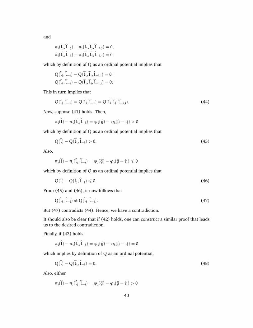
and

πi(lj, l−j) − πi(li, lj, l−i,j) = 0;

πj(li, l−i) − πj(li, lj, l−i,j) = 0;

which by definition of Q as an ordinal potential implies that

Q(lj, l−j) −Q(li, lj, l−i,j) = 0;

Q(li, l−i) −Q(li, lj, l−i,j) = 0;

This in turn implies that

Q(lj, l−j) = Q(li, l−i) = Q(li, lj, l−i,j). (44)

Now, suppose (41) holds. Then,

πi(l) − πi(li, l−i) = ϕi(g) −ϕi(g− ij) > 0

which by definition of Q as an ordinal potential implies that

Q(l) −Q(li, l−i) > 0. (45)

Also,

πj(l) − πj(lj, l−j) = ϕj(g) −ϕj(g− ij) 6 0

which by definition of Q as an ordinal potential implies that

Q(l) −Q(lj, l−j) 6 0. (46)

From (45) and (46), it now follows that

Q(li, l−i) 6= Q(lj, l−j). (47)

But (47) contradicts (44). Hence, we have a contradiction.

It should also be clear that if (42) holds, one can construct a similar proof that leadsus to the desired contradiction.

Finally, if (43) holds,

πi(l) − πi(li, l−i) = ϕi(g) −ϕi(g− ij) = 0

which implies by definition of Q as an ordinal potential,

Q(l) −Q(li, l−i) = 0. (48)

Also, either

πj(l) − πj(lj, l−j) = ϕj(g) −ϕj(g− ij) > 0

40

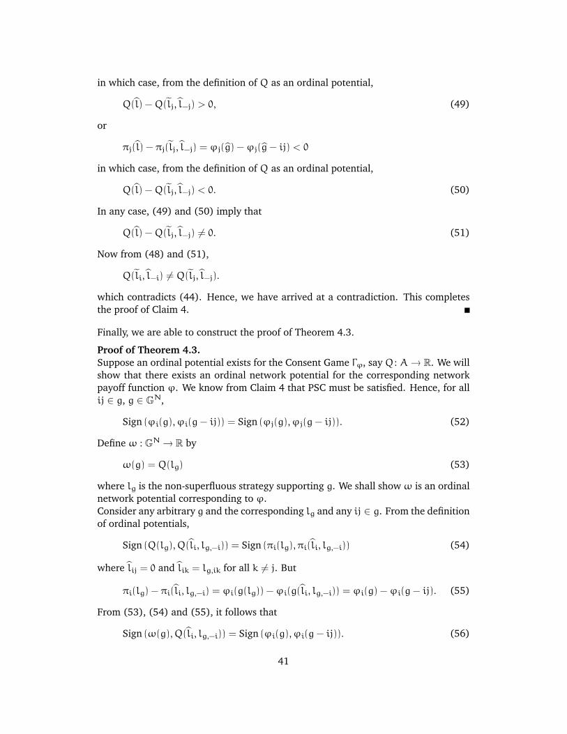
in which case, from the definition of Q as an ordinal potential,

Q(l) −Q(lj, l−j) > 0, (49)

or

πj(l) − πj(lj, l−j) = ϕj(g) −ϕj(g− ij) < 0

in which case, from the definition of Q as an ordinal potential,

Q(l) −Q(lj, l−j) < 0. (50)

In any case, (49) and (50) imply that

Q(l) −Q(lj, l−j) 6= 0. (51)

Now from (48) and (51),

Q(li, l−i) 6= Q(lj, l−j).

which contradicts (44). Hence, we have arrived at a contradiction. This completesthe proof of Claim 4.

Finally, we are able to construct the proof of Theorem 4.3.

Proof of Theorem 4.3.Suppose an ordinal potential exists for the Consent Game Γϕ, say Q : A → R. We willshow that there exists an ordinal network potential for the corresponding networkpayoff function ϕ. We know from Claim 4 that PSC must be satisfied. Hence, for allij ∈ g, g ∈ GN,

Sign (ϕi(g), ϕi(g− ij)) = Sign (ϕj(g), ϕj(g− ij)). (52)

Define ω : GN → R by

ω(g) = Q(lg) (53)

where lg is the non-superfluous strategy supporting g. We shall show ω is an ordinalnetwork potential corresponding to ϕ.Consider any arbitrary g and the corresponding lg and any ij ∈ g. From the definitionof ordinal potentials,

Sign (Q(lg),Q(li, lg,−i)) = Sign (πi(lg), πi(li, lg,−i)) (54)

where lij = 0 and lik = lg,ik for all k 6= j. But

πi(lg) − πi(li, lg,−i) = ϕi(g(lg)) −ϕi(g(li, lg,−i)) = ϕi(g) −ϕi(g− ij). (55)

From (53), (54) and (55), it follows that

Sign (ω(g),Q(li, lg,−i)) = Sign (ϕi(g), ϕi(g− ij)). (56)

41

Now, we claim that

Q(li, lg,−i) = Q(lg−ij) = ω(g− ij). (57)

We show this assertion as follows. First, by definition of ordinal potentials,

Sign (πj(li, lg,−i), πj(li, lj, lg,−i,j)) = Sign (Q(li, lg,−i),Q(li, lj, lg,−i,j)) (58)

where lj is such that lji = 0, ljk = lg,jk for all k 6= i. However,

πj(li, lg,−i) − πj(li, lj, lg,−i,j) = ϕj(g(li, lg,−i)) −ϕj(g(li, lj, lg,−i,j))

= ϕj(g− ij) −ϕj(g− ij) = 0. (59)

Also, (li, lj, lg,−i,j

)= lg−ij. (60)

Hence, by (58), (59), (60) and definition of ω, it follows that

Sign (πj(li, lg,−i), πj(li, lj, lg,−i,j)) = 0

=⇒ Sign (Q(li, lg,−i),Q(li, lj, lg,−i,j)) = 0

=⇒ Q(li, lg,−i) = Q(li, lj, lg,−i,j)

=⇒ Q(li, lg,−i) = Q(lg−ij) = ω(g− ij) (61)

which proves the claim.Finally, from (52), (56) and (57), it follows that

Sign (ϕi(g), ϕi(g− ij)) = Sign (ϕj(g), ϕj(g− ij)) = Sign (ω(g),ω(g− ij)).

This proves ω is indeed an ordinal network potential for ϕ.

Proof of Theorem 5.3

Claim 5 (Jackson and Watts 2001, Theorem 1A)If there exists a function w : GN → R such that [g′ defeats g] ⇐⇒ [w(g′) > w(g) andg and g′ are adjacent], then there are no improvement cycles.

With this we are able to show assertion 5.3(b).

Claim 6 If ϕ ∈ Φ3, then there are no improvement cycles.

Proof. We have to find a function w as defined in Claim 5. But such a function isgiven by the ordinal network potential ω. Hence, the result follows.

From this assertion we immediately arrive on assertion 5.3(a) as a corollary to Claim6.

42

Claim 7 If ϕ ∈ Φ3, then there exists at least one pairwise stable network for the corre-sponding network payoff function.

Proof. Follows from Lemma 5.2 and Claim 6.

With regard to assertion 5.3(c) we remark that PSC is sufficient to guarantee thatall strongly pairwise stable networks are strictly pairwise stable as well. Hence, weimmediately establish the desired assertion.This completes the proof of all three assertions stated in Theorem 5.3.

Proof of Theorem 5.5

In order to show Theorem 5.5, we use another result due to Jackson and Watts(2001).

Claim 8 (Jackson and Watts 2001, Theorem 1B)If the network payoff function satisfies no indifference and there are no improvementcycles, then there exists a functionw : GN → R such that [g′ defeats g] ⇔ [w(g) > w(g′)and g and g′ are adjacent].

To proceed with the proof of Theorem 5.5 we remark that by Claim 8, it followsthat since the network payoff function satisfies no indifference and there are noimprovement cycles, there exists a function w : GN → R such that [g′ defeatsg] ⇔ [w(g′) > w(g) and g and g′ are adjacent].

Suppose g′ defeats g. Then, it is either the case that

(i) g′ = g− ij with ϕi(g′) > ϕi(g), or

(ii) g′ = g+ ij with ϕi(g′) > ϕi(g)and ϕj(g′) > ϕj(g).

In both (i) and (ii), by PSC, ϕj(g′) > ϕj(g).Hence, [w(g) −w(g− ij) > 0 ] ⇔ [g defeats g− ij ] ⇔ [ϕi(g) −ϕi(g− ij) > 0 andϕj(g) −ϕj(g− ij) > 0 ].Also, [w(g) −w(g − ij) < 0 ] ⇔ [g − ij defeats g ] ⇔ [ϕi(g) − ϕi(g − ij) < 0 andϕj(g) −ϕj(g− ij) < 0 ].

Next, let w(g) − w(g − ij) = 0. Then neither g − ij defeats g nor g defeats g − ij

which is impossible by no indifference. Also, if ϕi(g) − ϕi(g − ij) = 0 and ϕj(g) −

ϕj(g− ij) = 0, again neither g− ij defeats g nor g defeats g− ij which is impossibleby no indifference.So it is trivially the case that [w(g) −w(g− ij) = 0 ] ⇔ [ϕi(g) −ϕi(g− ij) = 0 andϕj(g) −ϕj(g− ij) = 0 ].

Hence, by definition, w is an ordinal network potential, showing the assertion.

43

Proof of Theorem 5.6

For network payoff functions belonging to Φ2, we prove that a strongly pairwise sta-ble (and hence strictly pairwise stable) network exists by identifying those networksthat are supported through ordinal potential maximizing strategies in Γϕ. We showthat these particular networks form a strict subset of the set of strongly pairwisestable networks Ps(ϕ) = P∗(ϕ).

Claim 9 Let ϕ ∈ Φ2 be such that the Consent Game Γϕ = (A,π) admits an ordinalpotential function Q : A → R. if l ∈ A is such that Q(l) = Q(l ′) for all l ′ ∈ A, theng(l) ∈ Ps(ϕ).

Proof. Suppose that g = g(l) is such that l ∈ A maximizes the ordinal potentialfunctionQ on A. Now, assume by contradiction that g is not strongly pairwise stable.Then it is either not LAP or not SLDP. We shall show that both lead to contradictions.

First assume that g is not SLDP. This implies there exists a player i ∈ N and a set of itsneighbors M ⊂ Ni(g) such that ϕi(g\hM) > ϕi(g) where hM = {ij ∈ g|j ∈M} ⊂ g.Consider a strategy li such that lij = 0 for all j ∈ M and lij = lij for all j ∈ N\M.Then, g(li, l−i) = g\hM. This implies πi(li, l−i) > πi(l), which in turn implies thatQ(li, l−i) > Q(l). This contradicts the fact that l is a potential maximizer.

Next lets assume that g is not LAP. Then, there exists a pair i, j ∈ N such that ϕi(g+

ij) > ϕi(g) implies ϕj(g + ij) > ϕj(g). By Lemma 4, ϕj(g + ij) > ϕj(g). Now, giventhat ij /∈ g, there are three possibilities which we delineate as three cases. For eachof these cases we show a contradiction.

CASE 1: lij = 1, lji = 0

In this case, consider a strategy lj such that lji = 1, ljk = ljk for all k 6= i. Then,ϕj(g+ ij) > ϕj(g) ⇒ πj(lj, l−j) > πj(l) =⇒ Q(lj, l−j) > Q(l) by definition of ordinalpotentials which is a contradiction.

CASE 2: lij = 0, lji = 1

In this case, consider a strategy li such that lij = 1, lik = lik for all k 6= j. Then,ϕi(g+ ij) > ϕi(g) ⇒ πi(li, l−i) > πi(l) =⇒ Q(li, l−i) > Q(l) by definition of ordinalpotentials which is a contradiction.

CASE 3: lij = 0 = lji

Consider a strategy li such that lij = 1, lik = lik for all k 6= j. Then, πi(li, l−i) =

πi(l) = ϕi(g) ⇒ Q(li, l−i) = Q(l). Consider another strategy lj such that lji = 1,ljk = ljk for all k 6= i. Then, πj(li, lj, l−i,j) = ϕj(g + ij) > ϕj(g) = πj(li, l−i) ⇒Q(li, lj, l−i,j) > Q(li, l−i) = Q(l) which contradicts that l is a potential maximizer.

That completes the proof of the claim.

44