Network Decontamination using Cellular Automata Livaniaina Hary Rakotomalala Thesis submitted to the Faculty of Graduate and Postdoctoral Studies in partial fulfillment of the requirements for the Doctorate in Philosophy (Ph.D.) degree in Computer Science Ottawa-Carleton Institute for Computer Science School of Electrical Engineering and Computer Science University of Ottawa © Livaniaina Hary Rakotomalala, Ottawa, Canada, 2016

Welcome message from author
This document is posted to help you gain knowledge. Please leave a comment to let me know what you think about it! Share it to your friends and learn new things together.
Transcript

Network Decontamination using Cellular Automata
Livaniaina Hary Rakotomalala
Thesis submitted to the
Faculty of Graduate and Postdoctoral Studies
in partial fulfillment of the requirements
for the Doctorate in Philosophy (Ph.D.) degree in
Computer Science
Ottawa-Carleton Institute for Computer Science
School of Electrical Engineering and Computer Science
University of Ottawa
© Livaniaina Hary Rakotomalala, Ottawa, Canada, 2016

ii
Abstract
We consider the problem of decontaminating a network where all nodes are infected
by a virus. The decontamination strategy is performed using a Cellular Automata (CA)
model in which each node of the network is represented by the automata cell and thus, the
network host status is also mapped to the CA state (contaminated, decontaminating,
decontaminated). All hosts are assumed to be initially contaminated and the status of each
cell is synchronously updated according to a set of local rules, based on the state of its
neighbourhood. Our goal is to find the set of local rules that will accomplish the
decontamination in an optimal way. The metrics used to define optimality is the
minimization of three metrics: the maximum number of decontaminating cells at each step,
the required value of the immunity time of each cell and the number of steps to complete the
sanitization algorithm.
In our research, we explore the designing of these local decontamination rules by
refining the concept of the neighbourhood radius of CA with the addition of two new
dimensions: Visibility Hop and Contamination Distance. Additionally, a research tool that
help us manage our study have been developed.

iii
Ho anao
Tsy nitsahatra namporisika ahy

iv
Acknowledgment
I extend my sincere gratitude and appreciation to the people who made this thesis possible.
First of all, I am extremely grateful to my research guide, Prof. Nejib Zaguia for always giving me
his unrestrained encouragement. His valuable suggestions during the course of work are gratefully
acknowledged. This thesis would not have been possible without his help, support and patience. This
work is as much his creation as it is mine. I would also like to thank his family members despite my
too-many frequent visit at their home at random hours, often very early and sometimes very late;
though they have constantly made me feel that I was always welcome.
I would like to especially acknowledge the unwavering support of my wife Stephanie, whose
encouragement saw me past those times when my confidence and motivation faltered. I would also
like to thank my family for their unconditional support; I share this moment of pride and happiness
with them.
I am indebted to all reviewers who have gone through my work and helped me fill in the knowledge
gaps. I would also like to thank Dr Daniel Amyot for the help he is always willing to provide.
Last, I would like to acknowledge the support of the “University of Ottawa Excellence Scholarship”
and the “Fonds québécois de la recherche sur la nature et les technologies” (FQRNT) for partially
financing this thesis.
Sincerely,
Livaniaina Hary Rakotomalala

v
Contents
1. Introduction.................................................................................................................. 1 1.1. Problem Statement ................................................................................................ 1 1.2. Network Decontamination ................................................................................... 1
1.2.1. Decontamination by Mobile Agents ......................................................... 2
1.2.2. Network Topology and Graph approach .................................................. 2 1.2.3. The Cellular Automaton approach ............................................................ 3
1.3. Cellular Automata ................................................................................................. 3 1.3.1. Definition and structure ............................................................................ 3 1.3.2. Cellular Automata and network topology ................................................ 5
1.3.3. Decontamination using Cellular Automata .............................................. 6
1.4. Motivation and Pertinence .................................................................................... 7 1.5. Research Questions and Requirements ................................................................. 8
1.5.1. State of the art and challenges .................................................................. 8 1.5.2. Our research and contributions ............................................................... 10
1.6. Thesis Organization ............................................................................................ 10
2. Literature Review ...................................................................................................... 12 2.1. Network Decontamination and approach classification ..................................... 12
2.2. External Decontamination .................................................................................. 13 2.2.1. Graph Search and the Search Number .................................................... 13 2.2.2. Network Decontamination by Mobile Agents ........................................ 14
2.3. Internal Decontamination ................................................................................... 16
2.3.1. Decontamination using Cellular Automata ............................................ 17
2.3.2. 2D Cellular Automaton Neighbourhood ................................................ 17 2.3.2.1. The von Neumann neighbourhood ...................................................... 17
2.3.2.2. The Moore neighbourhood................................................................. 18 2.3.3. Basic Network Decontamination under CA ........................................... 19 2.3.3.1. Horizontal flow under the von Neumann neighbourhood .................. 19
2.3.3.2. Horizontal flow under the Moore neighbourhood ............................. 21 2.3.4. Network Decontamination under CA with Time Immunity ................... 21
2.3.4.1. Strategies under the von Neumann neighbourhood ............................ 21 2.3.4.2. Strategies under the Moore neighbourhood ........................................ 23
2.4. Theory of Cellular Automata .............................................................................. 24
2.4.1. Relevancy ............................................................................................... 24 2.4.2. Properties ................................................................................................ 25
2.4.3. Applications using Cellular Automata .................................................... 26 2.4.4. A selected review of simulation software ............................................... 27
3. The Model ................................................................................................................... 29 3.1. The Cellular Automaton model .......................................................................... 29
3.1.1. 2D CA as State space .............................................................................. 29 3.1.2. Network Host state as Transition State ................................................... 30 3.1.3. Decontamination algorithms as Cellular Automaton Transition Rules . 31 3.1.4. Conflicting rules and Non-determinism ................................................. 32

vi
3.2. New dimensions to the definition of a Cellular Automaton radius .................... 32
3.2.1. The Visibility Hop Vh ............................................................................. 33
3.2.2. The Contamination Distance Cd ............................................................. 33 3.2.3. Relationship between Vh and Cd ............................................................ 34
3.3. Recontamination and Immunity model .............................................................. 35 3.3.1. The contamination model ....................................................................... 35 3.3.2. The re-contamination model .................................................................. 36
3.3.3. The immunity model .............................................................................. 36 3.4. Terms and Notations ........................................................................................... 37
3.4.1. Transition state notation and representation in grayscale/color mode .... 38 3.4.2. New Neighbourhood configuration notation .......................................... 39
3.5. Complexity measures .......................................................................................... 41
4. Decontamination with Visibility Hop and Contamination Distance ..................... 42 4.1. General Concept ................................................................................................. 42 4.2. Basic Visibility Hop Vh=1 ................................................................................. 46
4.2.1. Contamination distance Cd=1................................................................ 46
4.2.2. Contamination distance Cd=2................................................................ 46 4.2.2.1. Grid topology ..................................................................................... 46
4.2.2.2. Circular grid topology ......................................................................... 49 4.3. The impact of a greater Visibility, case study of Vh=2 ...................................... 51
4.3.1. Contamination Distance Cd=1 ................................................................ 51
4.3.1.1. Grid topology ..................................................................................... 51 4.3.1.2. Circular grid topology ......................................................................... 52
4.3.2. Contamination Distance Cd=2 ................................................................ 53 4.3.2.1. Grid topology ...................................................................................... 53 4.3.2.2. Circular Grid topology ........................................................................ 56
4.4. Summary ............................................................................................................. 57
5. Diagonal Flow............................................................................................................. 59 5.1. Motivation ........................................................................................................... 59 5.2. Basic Case of Visibility Vh=1 ........................................................................... 60
5.2.1. Contamination Distance Cd=1 ................................................................ 61 5.2.2. Generalization of an arbitrary distance Cd=k ......................................... 63
5.3. The impact of a greater Visibility ( 2Vh ) on Diagonal Moves ...................... 67 5.3.1. Contamination Distance Cd=1 ................................................................ 67 5.3.2. Contamination Distance Cd=2 ................................................................ 68
5.4. Generalization for an arbitrary Cd and Vh ......................................................... 72 5.5. Summary ............................................................................................................. 74
6. Subdividing Strategies ............................................................................................... 77 6.1. Motivation ........................................................................................................... 77 6.2. Road Traffic Approach ....................................................................................... 78
6.2.1. Base Idea ................................................................................................. 78 6.2.2. Sample Execution ................................................................................... 79
6.2.3. The pattern retrieval ................................................................................ 79 6.2.3.1. The pattern retrieval with conserved decontamination flow ............... 82 6.2.3.2. The pattern retrieval with inverse decontamination flow ................... 84 6.2.4. Similar strategies on sub networks ......................................................... 90
6.3. Diagonal snake Approach ................................................................................... 95

vii
6.3.1. Base Idea ................................................................................................. 95
6.3.2. Sample Execution ................................................................................... 97
6.3.3. Division and Re-Application ................................................................ 104 6.3.3.1. Case with 2 corner initiators. ............................................................ 104 6.3.3.2. Case with 4 corner initiators. ............................................................ 108
6.4. The subdividing strategy of the Diagonal Move Approach ............................. 109 6.4.1. Case with 2 corner initiators ................................................................ 110
6.4.2. Case with 4 corner initiators ................................................................ 112 6.4.3. Case with 3 corner initiators ................................................................ 117 6.4.4. Rules minimization ............................................................................... 118 6.4.4.1. Approach by “flow analysis”. ........................................................... 119 6.4.4.2. Approach by “transition rules merge”. ............................................. 121
6.5. Summary ........................................................................................................... 122
7. CAEDISI, a CA editor and simulator for Network Decontamination ............... 124 7.1. Motivation ......................................................................................................... 124
7.1.1. Needs and existing software limitations ............................................... 124
7.1.2. Overall characteristics .......................................................................... 125 7.2. Caedisi versus current CA Software ................................................................. 127
7.2.1. CA Structure ......................................................................................... 127 7.2.2. Simulation properties ............................................................................ 131 7.2.3. Inverter and Reversability ..................................................................... 134
7.2.4. Database, Libraries and Software properties ........................................ 134 7.3. Software engineering approach ........................................................................ 136
7.3.1. Architecture and Technology ............................................................... 136 7.3.2. Functionality modules .......................................................................... 137
7.4. The main views ................................................................................................. 137
7.4.1. The Simulator wireframes and its functionalities ................................. 138
7.4.2. The CA Parameters wireframes and its functionalities ........................ 139 7.4.3. The Inverter wireframes and its functionalities .................................... 141 7.4.4. The Inverter-Parameter wireframes and its functionalities .................. 143
7.5. The Library Module .......................................................................................... 144 7.5.1. Pertinence and goals ............................................................................. 144
7.5.2. The Transition State Definition user interface ...................................... 144 7.5.3. The Neighbourhood Definition user interface .................................... 145
7.6. The Model ......................................................................................................... 146 7.7. The Simulator module ...................................................................................... 148
7.7.1. Pertinence and goals ............................................................................. 148
7.7.2. Application logic .................................................................................. 149
7.7.3. Simulation Metadata ............................................................................. 149
7.8. Rules Validation & (Non) determinism ............................................................ 151 7.8.1. The transition rule collision validation ................................................. 151 7.8.2. The transition rule inclusion validation ................................................ 153 7.8.3. Validation Rules algorithm ................................................................... 154
7.9. The Inverter module ........................................................................................ 155
7.9.1. Pertinence and goals ............................................................................. 155 7.9.2. Application logic .................................................................................. 156 7.9.3. Miscellaneous notes .............................................................................. 158

viii
8. Summary & Future work ....................................................................................... 160 8.1. Summary ........................................................................................................... 160
8.2. Current work extension and Future work ......................................................... 161
Bibliography ................................................................................................................... 164
Appendix A: Implementation of the Simulation algorithm
Appendix B: Implementation of the Inverter (without immunity) algorithm
Appendix C: Implementation of the Inverter (with immunity) algorithm
Appendix D: Implementation of the rules collision/inclusion validation algorithm
Appendix E: Implementation of the contamination rules generation algorithm
Appendix F: Implementation of the recursive generation of neighbourhood data

ix
List of Figures
Figure 1.1: The native representation of a CA grid ................................................................. 4 Figure 1.2: Sample of topologies that can be modeled by a 1-dimensional CA: Chain(a),
Ring(b), Chordal Ring (c) and Complete Graph (d). .............................................. 5 Figure 1.3: Sample of topologies that can be modeled by a 2-dimensional CA: Rectangle
Grid (a), Circular Grid (b), Torus (2D view (c) and its 3D representation (d)) .... 6 Figure 1.4: An example of a 2D grid network modeled by a Cellular Automaton .................. 7 Figure 1.5: Two examples of attempted decontamination of a 2-dimensional CA .................. 9
Figure 2.1: The omni standard neighbourhood: the von Neumann neighbourhood and the
Moore neighbourhood. ......................................................................................... 17 Figure 2.2: The process of decontaminating basic CAs under the von Neumann
neighbourhood (source [Daa12]) .......................................................................... 20
Figure 2.3: The process of decontaminating circular CAs under the von Neumann
neighbourhood and its local rules (source [Daa12]) ............................................. 20
Figure 2.4: The circular propagation of an internal decontamination .................................... 21 Figure 2.5: Propagation of k decontaminating cells with Temporal Immunity in CAs with
von Neumann neighbourhood (source [DFZ10]) ................................................. 22
Figure 2.6: Propagation of decontaminating cells with Temporal Immunity in basic CAs
under the Moore neighbourhood (source [DFZ10]) ............................................. 23
Figure 2.7: Propagation of decontaminating cells with Temporal Immunity in circular CAs
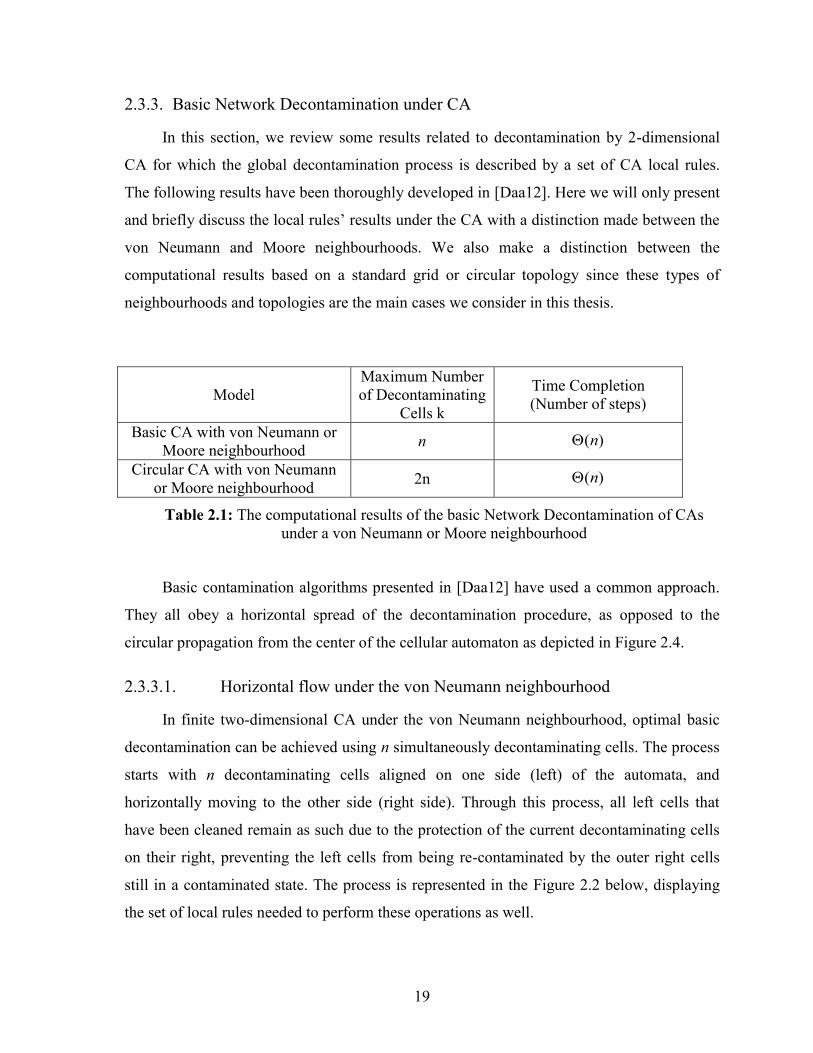
under Moore neighbourhood (source [DFZ10]) .................................................. 24 Figure 2.8: A partial execution of Conway’s Game of life ................................................... 27
Figure 3.1: A representation of the von Neumann and Moore neighbourhood when the
radius distance is equal to 2. ................................................................................. 32
Figure 3.2: New edges inserted resulting to a new graph topology when Vh=2 under the von
Neumann neighbourhood. ..................................................................................... 34
Figure 3.3: A sample of the new notation of a transition rule using a grayscale or color visual
representation of the neighbourhood. ................................................................... 40
Figure 4.1: The decontamination block .................................................................................. 43 Figure 4.2: A sample execution of the left-to-right basic decontamination under the von
Neumann neighbourhood in a finite CA when Vh=1 and Cd=2 ........................... 47
Figure 4.3: A sample execution of the left-to-right basic decontamination under the von
Neumann neighbourhood in a circular CA when Vh=1 and Cd=2 ...................... 49
Figure 4.4: The propagation flow of the basic decontamination under the von Neumann
neighbourhood in a circular CA .......................................................................... 50 Figure 4.5: A sample execution of the left-to-right decontamination under the von Neumann
neighbourhood in a circular CA when Vh=2 and Cd=1 ...................................... 52
Figure 4.6: Propagation of a 2 by 2 column decontamination under the von Neumann
neighbourhood when Vh=2 and Cd=2 .................................................................. 55 Figure 5.1: A basic propagation of a decontamination approach initiated by an inner cell
showing a bound-less number of decontaminating cells ...................................... 60 Figure 5.2: Propagation of the basic diagonal move under the von Neumann neighbourhood
when Vh=1 and Cd=1 ........................................................................................... 61 Figure 5.3: Propagation of the basic diagonal move under the von Neumann neighbourhood
when Vh=1 and Cd=k ........................................................................................... 63

x
Figure 5.4: Maximum Number of Decontaminating cells in a diagonal move within the von
Neumann Neighbourhood when Vh=1 and Cd=k ................................................. 65
Figure 5.5: Propagation of the diagonal move under the von Neumann neighbourhood when
2Vh and Cd=2 .................................................................................................. 68 Figure 5.6: Propagation of the diagonal move under the von Neumann neighbourhood when
Vh=Cd=k ............................................................................................................... 72
Figure 6.1: The road traffic approach ..................................................................................... 78 Figure 6.2: Propagation of the road traffic approach under the von Neumann neighbourhood
.............................................................................................................................. 79 Figure 6.3: The two different possibilities of finding the initial case in the Road Traffic
approach ................................................................................................................ 80
Figure 6.4: Counterexample of configuration during the Road Traffic approach when Vh=2
.............................................................................................................................. 85
Figure 6.5: The cut strategy of the road traffic approach ....................................................... 90 Figure 6.6: The diagonal snake approach within the Moore neighbourhood ......................... 95 Figure 6.7: Execution difference around the diagonal depending on the value of n .............. 97 Figure 6.8: Propagation of the diagonal snake approach within the Moore neighbourhood . 98
Figure 6.9: The different type of cells within the CA during the diagonal snake strategy ... 100 Figure 6.10: An attempt to define f1 within the diagonal snake strategy .............................. 101 Figure 6.11: The subdividing strategy using 2 initiators. ..................................................... 105
Figure 6.12: The subdividing strategy using the snake approach with 4 initiators .............. 109 Figure 6.13: The divide and conquer diagonal strategy with 2 initiators ............................. 111
Figure 6.14: The subdividing strategy using diagonal move with 4 initiators ..................... 114 Figure 6.15: A sample of execution of the subdividing strategy using diagonal move
algorithm using a dynamic number of initiators. ................................................ 118
Figure 7.1: The CAEDISI software architecture .................................................................. 136
Figure 7.2: The simulator home screen ................................................................................ 138 Figure 7.3: The CA parameters screen of the simulator module .......................................... 139 Figure 7.4: The inverter home screen ................................................................................... 141
Figure 7.5: The CA parameter screen of the inverter module .............................................. 143 Figure 7.6: The Transition State Definition screen of the library module showing the current
list of cell state types. .......................................................................................... 144 Figure 7.7: The Neighbourhood Definition edit screen of the library module showing how to
create a new type of neighbouhood .................................................................... 145 Figure 7.8: the data entity model of CAEDISI ..................................................................... 146
Figure 7.9: A sample view of the metadata screen of the simulation module ...................... 149 Figure 7.10: An example of two rules having collision errors ............................................. 151 Figure 7.11: A view of the Rules Validation Results screen showing collision errors ........ 152
Figure 7.12: An example of two rules having inclusion errors ............................................ 153 Figure 7.13: A view of the Rules Validation Results screen showing inclusion errors ....... 154 Figure 7.14: An example of the Inverter execution showing the creation of rules .............. 157 Figure 7.15: The impact of an even/odd sized CA on the Inverter....................................... 158

xi
List of Tables
Table 2.1: The computational results of the basic Network Decontamination of CAs under a
von Neumann or Moore neighbourhood................................................................ 19 Table 2.2: The computational results of the Network Decontamination under the von
Neumann neighbourhood and with Time Immunity ............................................. 22 Table 2.3: The computational results of the Network Decontamination under the Moore
neighbourhood and with Time Immunity .............................................................. 24
Table 3.1: Various notations of the transition state of a CA in current literature and in this
thesis. ..................................................................................................................... 38 Table 4.1: Rule for Basic decontamination in Finite CA under the von Neumann
neighbourhood when Vh=1 and Cd=2 ................................................................... 48 Table 4.2: Alternative Rule for Basic decontamination in Finite CA under the von Neumann
neighbourhood when Vh=1 and Cd=2 ................................................................... 49
Table 4.3: Rule for Basic decontamination in circular CA under the von Neumann
neighbourhood when Vh=1 and Cd=2 ................................................................... 51
Table 4.4: Rule for Basic decontamination in Finite CA under the von Neumann
neighbourhood when Vh=2 and Cd=1 ................................................................... 52 Table 4.5: Rule for Basic decontamination in a circular and Finite CA under the von
Neumann neighbourhood when Vh=2 and Cd=1 .................................................. 53 Table 4.6: Rule for Basic Decontamination in Finite CA under the von Neumann
neighbourhood when Vh=2 and Cd=2 ................................................................... 56 Table 4.7: Rule for Basic Decontamination in Finite CA under the von Neumann
neighbourhood when Vh=2 and Cd=2 ................................................................... 57
Table 4.8: Summary of the basic decontamination results for a n*m )( mn CA under the
topology, Visibility Hop and Contamination Distance parameters. ...................... 58 Table 5.1: Rules for decontamination in Finite CA using basic diagonal move under the von
Neumann neighbourhood when Vh=1 and Cd=1 .................................................. 62 Table 5.2: Rules for Basic Decontamination in Finite CA using diagonal move under the von
Neumann neighbourhood when Vh=1 and for an arbitrary Cd=k ......................... 67
Table 5.3: Rules for Basic Decontamination in Finite CA using diagonal move under the von
Neumann neighbourhood when Vh=2 and Cd=2 .................................................. 70 Table 5.4: Another possible set of rules for Basic Decontamination in Finite CA using
diagonal move under the von Neumann neighbourhood when Vh=2 and Cd=2 ... 71
Table 5.5: Summary of decontamination results of an n*m (nm) CA using Diagonal move
strategies. ............................................................................................................... 76 Table 6.1: Rules for Basic Decontamination in Finite CA using the Road Traffic approach
(with flow conservation) under the von Neumann neighbourhood with Vh=3 ..... 84 Table 6.2: Rules for Basic Decontamination in Finite CA using the Road Traffic approach
with inverse flow under the von Neumann neighbourhood with Vh=3 ................. 87 Table 6.3: Rules for Basic Decontamination in Finite CA using the road Traffic approach
(with inverse flow) under the Moore neighbourhood with Vh=2 ......................... 90 Table 6.4: Rules for Decontamination in Finite CA using the road traffic approach (with
inverse flow) using 2*k decontaminating cells under Moore neighbourhood with
Vh=2 ....................................................................................................................... 93 Table 6.5: Direction flow of the decontaminating transition state ......................................... 99

xii
Table 6.6: Rules for Decontamination in Finite CA using the diagonal snake approach move
under the Moore neighbourhood when Vh=2 and for an immunity time It=2n-1
............................................................................................................................. 104 Table 6.7: Rules for Decontamination in Finite CA using the diagonal snake approach move
with 2 corner initiators under the Moore neighbourhood of Vh=2. ..................... 107 Table 6.8: Rules for Basic Decontamination in Finite CA using basic diagonal move and two
corner initiators under the von Neumann neighbourhood when Vh=1 and Cd=1
............................................................................................................................. 112 Table 6.9: Rules for Basic Decontamination in Finite CA using basic diagonal move and
four corner initiators with the von Neumann neighbourhood when Vh=1 and
Cd=1 .................................................................................................................... 117 Table 6.10: Alternative rules for Basic Decontamination in Finite CA under the von
Neumann neighbourhood using basic diagonal move and initiated by the top left
initiator when Vh=1 and Cd=1 ............................................................................. 119 Table 6.11: Alternative rules for Basic Decontamination in Finite CA with the von Neumann
neighbourhood using basic diagonal move and initiated by any corner initiators
when Vh=1 and Cd=1 .......................................................................................... 121 Table 6.12: Summary of decontamination results of a n*n CA using the Road Traffic,
Diagonal Snake and Diagonal Move strategy. .................................................... 123 Table 7.1: CAEDISI vs current CA Software (Overall structure) ........................................ 128 Table 7.2: CAEDISI vs current CA Software (Simulation properties) ................................ 132
Table 7.3: CAEDISI vs current CA Software (Inverter and Reversability) ......................... 134 Table 7.4: CAEDISI vs other CA Software (Database and Libraries) ................................. 135

1
Chapter 1
1. Introduction
1.1. Problem Statement
Consider a network where sites (nodes) are processing some computations. In addition,
sites can communicate with each other through links. A very realistic situation is that some
sites might be contaminated, for example, by a virus. These infections could have been
inserted locally in the network or by external network attacks. When infected these nodes
usually behave incorrectly. Typically, antivirus programs are run at each infected network
site for disinfection. However, there is no genuine guarantee that the clean site will not be re-
infected again. To accentuate the issue, a network site cannot detect the presence of viruses
within itself and therefore cannot curb the spread of viruses. This situation is exploited by
some types of viruses which are capable of encouraging infected nodes to propagate the fault
to neighbouring nodes. The evident solution to execute the antivirus against all existing hosts
of the network is not an acceptable one because when active, it is assumed that the antiviral
program will reduce or even stop local computation and therefore disrupt the entire network.
In order to sanitize the network, a system must be capable of firstly, cleaning the infected
hosts and secondly, counteracting the propagation of faults. Network Decontamination is the
research of strategies for network sanitation by considering these previous two key points.
1.2. Network Decontamination
The Network Decontamination problem was first introduced in Speleology, where a
maze of caves was infected by gas and needed to be decontaminated [Bre67]. In computer
science, Network Decontamination is a field of study that addresses the problem of
sanitizing a network which is contaminated by a virus. A virus is assumed to be a program
that, when executed against a clean host, will make the host faulty. The faulty host then
spreads the virus over the network using communication links. A network is considered
contaminated by a virus when either one or more machine hosts are infected by a virus.
Infected hosts expose faulty behaviors and can contaminate neighbouring hosts which

2
recursively affects the entire network. In the decontamination problem, it is generally
assumed that the network is partially or fully contaminated. Our interest is to find an
efficient strategy to correct every faulty node by executing an antivirus against contaminated
hosts.
1.2.1. Decontamination by Mobile Agents
The most popular approach to sanitizing a distributed network is the use of Mobile
Agents. Mobile Agents are extensively used in distributed systems to solve typical problems
such as Rendez-vous, Graph Exploration and Black Holes. A listing of the use of Mobile
Agents in Distributed systems is found in [KK07]. Mobile Agents can be defined as software
entities with the capacity for motion inside a network and which can act on behalf of their
user with some degree of autonomy in order to accomplish different computing tasks.
Mobile Agents have been found to be useful in a number of network security applications
including Network Decontamination. The nature of the network topology plays an
important role in the efficiency of operations executed within the network by the sites and
the Mobile Agents (see [FHL06], [FHL08] and [FHL07]).
1.2.2. Network Topology and Graph approach
The standard visual way to represent a network is by the means of a graph: hosts are
represented by nodes, and the presence of edges between two nodes stipulates that there is a
connection link between these two hosts. Researchers have shown tremendous interest in the
debate over the best graph topology on which to model a network. Among the known
topologies are Ring, Tree, Rectangular Grids (or Mesh), Hypercube and Complete graphs.
Clearly, the choice of the topology has a direct impact on the efficiency of operations that
will be executed under the network. For instance, an optimal decontamination strategy
against a Ring network might not necessarily be efficient, nor even meaningful, for a
Complete graph.
Most solutions for graph theory problems such as graph coloring, covering problems
(e.g., Vertex cover), and route problems (e.g., Hamiltonian path, spanning tree) are
frequently used as the backbone of solutions in distributed systems problems such as Voting,
Leader Election, Broadcasting, or Routing. The Network Decontamination problem is
related, under certain conditions, to that of the graph search ([Mes08]). Thus, several of the

3
techniques and models considered by researchers for the general graph search problems are
quite useful in the study of the Network Decontamination problems when the network is
modeled by a graph.
1.2.3. The Cellular Automaton approach
In our thesis, we take a tangent direction from the graph approach. Instead of having
the external intervention of Mobile Agents cleaning the network, we put our focus on
finding "local" strategies so that hosts can trigger and execute the decontamination
themselves. The idea of using local approaches is known in distributed systems. Distributed
and networked systems often employ local majority based rules to enhance reliability and
fault-tolerance. Local voting schemes are used as decision tools in a variety of different
applications, for example, agreement and consensus in distributed systems. Also, systems
employing majority-based local voting schemes are known to have a higher level of
resistance. (For instance, one can use a similar idea with respect to network contamination in
which a clean cell is always immune to contamination as long as a majority of its neighbours
are uncontaminated). More precisely, we want to build local rules that will be applied to
each network site in a uniform way. To this end, we use a Cellular Automaton to model both
the network and the operations that need to be performed. Invented by Ulam and Neumann
in the 1950s, Cellular Automaton was originally used to study their joint work on liquid
motion for self-organizing and reproducing behaviors [Neu51]. Our motivation is based on
the fact that it is a discrete model known for its simplicity in integrating a locally based
voting scheme, yet powerful enough to model any complex application. The study of its
properties and its behavior has interested various disciplines as diverse as physics, biology,
and theoretical computer science (e.g. [ADF07], [Kar05], [CD98], [LM10]).
1.3. Cellular Automata
1.3.1. Definition and structure
A Cellular Automaton (CA) consists of a regular grid of cells, each having a finite
number of states (A formal definition of a CA can be consulted in Chapter 3). The grid can
be in any finite number of dimensions but the most used in practical applications are the 1-
dimensional and 2-dimensional ones (see Figure 1.1). For each cell, a set of cells, called

4
its neighbourhood, is defined relative to the specified cell. Neighbours are usually composed
by a set of cells surrounding the centered cell itself within a specific integer distance called
radius. An initial state is selected by assigning a state for each cell. A new generation is
created at the next step according to a fixed transition rule that determines the new state of
each cell in terms of the current state of the cell and the states of the cells in its
neighbourhood. Typically, the rule for updating the states of cells is the same for each cell,
does not change over time, and is applied to the whole grid simultaneously, which makes the
execution of the state update in a synchronous fashion.
1-dimensional CA
i i+1i-1
2-dimensional CA
i-1,j-1 i-1,j i-1,j+1
i,j-1 i,j i,j+1
i+1,j-1 i+ 1, j i+1,j+1
Figure 1.1: The native representation of a CA grid
The most elementary model of a CA is the 1-dimensional version (1D) (see Figure
1.1). Each site or cell in the lattice is in either the ON (a filled circle in the cell) or OFF (an
empty cell) state. In the example illustrated here, the site i-1 is OFF and the sites i and i+1
are ON. Each cell can have two states; therefore, there are 23= 8 possible configurations of
this neighborhood. For the CA to work, it is necessary to define what the state should be in
the next generation. Consequently, there are 28 = 256 possible local rules with a wide range
of behaviours and properties. The diversity of these simple rules alone has raised great
interest and contributes to its popularity since its introduction.

5
1.3.2. Cellular Automata and network topology
(a)
(b)
(c) (d)
Figure 1.2: Sample of topologies that can be modeled by a 1-dimensional CA:
Chain(a), Ring(b), Chordal Ring (c) and Complete Graph (d).
Network topology addresses how the various elements of a computer network are
arranged and graphs are useful because they serve as mathematical models of network
structures. The topological structure of a network can be depicted physically (how various
component such as the location of the device or cables are placed); or logically (how the data
flows within the network regardless of its physical design). In a CA, the physical topology of
the network can be a ring, a mesh or a torus and the dataflow between the components
which determines the logical topology of the network is addressed by the CA
neighbourhood. Indeed, CA has ability to model some specific classes of network
topologies. For instance, it is easy to see that a chain is naturally modeled by a 1-
dimensional CA. To this end, the chain is only extrapolated by a single array (see Figure
1.2a). Chorded rings are also special type of 1-dimensional circular CA (see Figure 1.2c). A
chordal ring },,...,2,1{ kpC of size n is a ring on n nodes 110 ,...,, nxxx where each node ix
is connected to nodes npini xx mod)(mod)1( ... and nkix mod)( . In a general aspect, a chordal ring
can be considered as a k-neighbours 1-dimensional circular CA. Note that when 1 kp ,
the chordal ring is a simple Ring (see Figure 1.2b) and becomes a Complete graph when
2
nkp (see Figure 1.2d).

6
(a) (b)
(c) (d)
Figure 1.3: Sample of topologies that can be modeled by a 2-dimensional CA:
Rectangle Grid (a), Circular Grid (b), Torus (2D view (c) and its 3D representation (d))
Additionally, rectangle grid (mesh) and possible variations can naturally be modeled
by a 2-dimensional (2D) CA (Figure 1.3a). When making a circular connection between the
various extremities of the 2D grid, the bi-dimensional CA with circular connections become
a Torus (Figure 1.3c). In fact, a 2D CA can model any instance of a grid as long as the
connections between elements follow a regular pattern that can be represented by the CA
neighbourhood concept. A 2D CA can represent a grid network with larger connections
between hosts in a larger neighbourhood defined in the CA. Figure 1.4 is an example of the
modelling of a simple sub-network by a 2D CA. In this example, a cell has a maximum of
six neighbours.
1.3.3. Decontamination using Cellular Automata
The use of a CA to perform the decontamination is possible under two conditions. The
first hypothesis is that the network must be modeled by a CA. In the previous section, we

7
have shown some candidate topologies that satisfy this condition. The second condition
concerns the state of the network sites that has to be mapped with the CA transition states.
To this end, each CA’s cell state is just set to one of these three states: Contaminated (the
network site is infected by a virus), Decontaminating (The network site is executing the
antiviral program) and Decontaminated (the virus has been removed from the network site
and the site is currently clean). The decontamination goal is to study the building of
transition rules that take as input a contaminated CA, and transfer each cell state from a
faulty contaminated state into a decontaminating state so that each cell eventually becomes
and remains decontaminated. An illustration of an execution is shown in Figure 1.4.
Contaminated network sites (white cell) are represented by the number "1" in the CA while
decontaminated cells are represented by "0" to represented the clean site (gray cell). When
cells are in a decontaminating state, it is represented by a dot "•" within both the CA and the
network graph representation.
Network using a graph representation
CA Representation
1 1 • 0 0 0
1 1 • 0 0 0
1 1 • 0 0 0
1 1 • • • •
1 1 1 1 1 1
Figure 1.4: An example of a 2D grid network modeled by a Cellular Automaton
1.4. Motivation and Pertinence
In a world dominated by networking and its ramifications (Internet, social networks,
distributed systems, distributed data, and cloud computing), networking reliability is crucial.
Similar to software which cannot be bug free, any networking system cannot insure
complete reliability. Indeed, network systems are now facing an increased number of attacks
than they have faced in the past. The problem is that faulty network sites become vulnerable
and can expose security holes. There are various types of breakdown including process
deaths, machine crashes, and network failures. A great concern for fault tolerance and

8
security is how to devise strategies to correct the faulty behaviour at network sites and to
control the propagation of faults. Thus, Network Decontamination has attracted many
researchers in the past decade. They have approached the Network Decontamination
problem from many angles including its empirical version of a fully contaminated network
that needs a full decontamination.
1.5. Research Questions and Requirements
1.5.1. State of the art and challenges
The general result within the field of Network Decontamination using external
approach is that the problem of determining the optimal number of mobile agents necessary
to perform the decontamination in arbitrary topologies is NP-hard. To date, much research
has been done on the study of the decontamination problem, especially in the theoretical
field of fault tolerance within distributed systems theory. There are a considerable number of
papers that have been published on the topic. Many researchers have studied the
decontamination problem under different types of parameters; however, most have
concentrated their efforts in the study of decontamination in topologies of graphs, such as
Trees, Rings, Tories, and Hypercubes. There are a few papers in which the network is
modelled by a CA.
With respect to pure CA theory, there are a number of papers devoted primarily to its
structure and its properties. There are also a considerable number of applications that
directly use CA as a backbone. That said, the amount of research that has been done
regarding the use of CA in the field of Network Decontamination is still limited.

9
t=0 t=1 t=2
(a)
(b)
Figure 1.5: Two examples of attempted decontamination of a 2-dimensional CA
One trivial decontamination strategy using a CA is to initially run the antiviral
program to one or multiple cells (initiators) of our CA and to propagate the decontamination
strategy to all existing neighbours (Figure 1.5a). This strategy is simple because it just
possesses two rules. The first rule suggests that any decontaminating cell gets
decontaminated at the next stage. The second rule proposes that any contaminated state in
contact with a decontaminating cell will also run the antiviral program in the next stage.
With this solution, we can see that the CA eventually gets fully decontaminated. However,
the fundamental issue with this solution is that the number of decontaminating cells
considerably increases at each step and therefore is boundless. If one attempt to reduce the
number of decontaminating cells at each step, a possible strategy would only propagate the
decontamination from the initiator cells to a limited number of neighbours, for instance to
the neighbours located on its right (as in Figure 1.5b). However, with this strategy, any
decontaminated cell will get re-contaminated by its left neighbours. These examples show
the nature of some problems that must be taken into account when building decontamination
strategies.

10
1.5.2. Our research and contributions
Our research focuses on the Network Decontamination problem using the concept of
CA. We propose optimal strategies to decontaminate a network using local rules by using a
2-dimensional CA as a model. Various basic algorithms using this type of model have been
investigated in [Daa12]. In this thesis, we continue this line of research by studying new
strategies under new assumptions. More precisely, we study the decontamination problem
under two new dimensions arising from the concept of radius within CA. To this date, only
direct neighbourhood (radius=1) have been considered. Therefore,
a new model of accessing knowledge information, which we define as Visibility Hop, is
proposed. This property allows a cell to oversee a larger neighbourhood.
a new model of (re)infections, which we define as Contamination Distance, is also
proposed. This property allows us to define which distant infected neighbours can
contaminate cleaned cells.
We demonstrate that the addition of these parameters brings new dynamics to the
decontamination process. The Visibility Hop allows us to discover new decontamination
strategies. Moreover, the Contamination Distance allows us to differentiate the strategies to
take under weaker or stronger conditions. Also fundamentally, a greater value assigned to
these properties also implies that the graph topology covered by the CA is denser than a
simple rectangle grid. These dynamics are seen in more details in Chapter 3.
Principally in this thesis, we developed several decontamination techniques under
these parameters. Additionally, a research tool that help us manage our research have been
developed.
1.6. Thesis Organization
This thesis is organized as follows.
In Chapter 2, we review the existing literature on the Network Decontamination
problem. We also briefly present some related results on CA which are significant to our
study.
Chapter 3 presents the model we will use in this thesis. We will also present the
terminology and other formal characterization of the various entities used in our document.

11
In Chapter 4, we investigate the impact of the Visibility Hop and Contamination
Distance against some basic known decontamination algorithms under a CA. We present the
result of our initial studies against this new concept under the von Neumann and Moore
neighbourhoods.
In Chapter 5, we present a new approach called Diagonal Flow and we show that the
concept of Visibility can bring noticeable improvement against these schemes.
In Chapter 6, we present others schemes of decontaminating a CA by using a
subdividing strategy similar to divide and conquer methods. We also show that the diagonal
move presented in the previous chapter can serve as a base block in this strategy.
In Chapter 7, we present a research tool that we have implemented that aims to assist
us in the study of Network Decontamination using CA.
In Chapter 8, we give a summary of the work accomplished so far and we present a
non exhaustive list of possible future work.

12
Chapter 2
2. Literature Review
In this chapter, we give a survey of the known problems and results related to our work in
this thesis. We briefly discuss the two different classifications of network decontamination
with respect to the approach being internal or external. We review known results for each
approach, especially when decontamination is performed by Mobile Agents. Then, we
outline in detail the current known algorithms and results of internal decontamination using
a CA as this is directly related to our study. We continue by enunciating some relevant
properties of the theory of CA. We conclude the chapter by listing some various applications
using CA.
2.1. Network Decontamination and approach classification
Network Decontamination is a widely studied problem in Computer Science. Network
hosts or sites are assumed to be contaminated by malicious software and a process needs to
be executed to clean the network. The process of decontamination is generally classified by
two distinct aspects. Depending on whether the decontamination is carried out by the
majority-voting mechanism already in place or by the use of a team of mobile agents, the
decontamination process is called internal or external, respectively. The process is called
internal due to the fact that the decontamination is processed by the sites themselves by
using local rules and without any outside intervention. An example of an internal process is
when the network is modeled by a CA and the local rules are composed of a set of transition
rules in which each cell obeys in exactly the same fashion. The process is called external
when the decontamination is processed by external entities to the system. An example of an
external decontamination is the cleaning by means of Mobile Agents. [Flo09] presents a
survey of the different methods of Network Decontamination with respect to these two
different approaches. In this chapter, we give a survey of the most common problems and
results related to our work in this thesis.

13
2.2. External Decontamination
2.2.1. Graph Search and the Search Number
The Network Decontamination problem is closely related to the graph search problem.
The metaphorical rendition of the two concepts has been introduced by Breisch in [Bre67].
The problem was presented as follows. A person is lost in a totally dark cave and the goal is
to find an efficient way to search and rescue the lost person. The author aims to find the
minimum number of searchers required to explore the cave so that it is impossible to miss
the victim. The analogy to the graph search problem is that the cave can be represented by a
finite connected graph G so that rooms are represented by vertices and the passages by
edges. The problem has been reformulated by other authors replacing the notion of the lost
person with an intruder, motivated by the fact that in the new problem, there are assumptions
that the intruder can have knowledge of the searchers' every move. Additionally, the intruder
is arbitrarily fast, invisible to rescuers, and even tries to avoid meeting the searchers
([Par78], [Par76]). Theoretically, we are given a graph ),( EVG with contaminated edges
and via a sequence of steps, one that uses searchers. The goal is to arrive at a situation where
all edges of the graph are simultaneously clean. More precisely, the problem is to find the
minimum number of searchers needed to clean the graph and to reach a final stage where all
edges are simultaneously clean. A clean edge Ee is immune to recontamination on two
conditions: either another searcher remains in a vertex adjacent to the edge, or all other
edges incident to this vertex are clean. That is, e is re-contaminated if there exists a path P
between e and a contaminated edge and there is no searcher residing in any node v for
Pv . An edge Eyxe ),( gets decontaminated if a searcher traverses it from x or y (or
from y to x). Any decontamination strategy can be broken down into a sequence of 3 basic
operations: the action of putting a searcher on a node v, the action of removing a searcher
from a node v, and the action of making the searcher traverse an edge e. Graph searching is
about finding a sequence composed of these three basic operations that results in all edges
being simultaneously clean. In general, researchers are most interested in finding optimal
search strategies and the minimization of the number of searchers used by a strategy.
Assuming a search strategy exists, )(Gs is the smallest number of searchers for a graph G.
Two results are important with respect to the search number. First, Meggido et al shows in

14
[MHG+88] that determining the search number of a graph is NP-hard. Second, LaPaugh
[Lap93] has proven that for every G, there is always a monotone search strategy that uses
)(Gs searchers. By definition, a search strategy is monotone if no recontamination ever
occurs. Several techniques and models considered by researchers with respect to the graph
search problem are useful in the study of the Network Decontamination problems.
2.2.2. Network Decontamination by Mobile Agents
The decontamination framework that has received great interest in recent years is
Network Decontamination using mobile agents. In computer science, a mobile agent is a
software entity that has the ability to move from node to node in a distributed system.
Mobile agents have been used in solving many distributed systems problems because of their
ease of use, their efficiency, and their fault-tolerance as explained in [KK07]. There are
several papers on the use of mobile agents in distributed systems problems including graph
exploration, black hole search and rendez-vous.
Decontamination by a mobile agent is considered an external decontamination because
the cleaning process is performed by an entity which is external to the system. The
decontamination process usually works in the same way. At any time, nodes can be
contaminated, clean, or guarded (if they contain at least an agent). All nodes are initially
contaminated except for one (the homebase) where a team of mobile agents is located.
Agents can move in the network from a node to a neighbouring node, and a contaminated
node is transformed into clean when an agent passes by the node. The goal is to reach a state
in which all nodes are clean (or guarded). Mobile agents are self-contained programs that
can move from a node to a neighbouring node to execute tasks independently of each other,
or to cooperate to solve problems. The network is still seen as an environment where nodes
represent hosts, edges represent connections between hosts, and we assume that the network
is initially contaminated. The goal is to deploy a team of agents to decontaminate the
network. An agent is a program that can migrate on the network. When an agent resides on a
node, it can detect all intruders at the node and clean the node if it is contaminated.
However, when a clean node has a contaminated neighbour, it becomes contaminated as
well. It is assumed that the agents start from the same node (the homebase) and can move to
neighbouring nodes. An important fact is that the problem of determining the optimal

15
number of agents necessary to perform the decontamination in arbitrary topologies is NP-
hard. Several papers exist about the optimal strategy to clean a network using mobile agents
under specific network topologies [FHL06], [LPS06], [LPS07], [FHL08], [FHL07].
In [FHL07], Flocchini et al consider the problem of decontaminating a network using
a team of mobile agents. The agents can clean a node after the agent transits the node. When
an agent transits a node, it can clean it, but when the node is left unguarded, it will be re-
contaminated as soon as at least one of its neighbours is contaminated. The authors' focus is
on asynchronous chordal ring networks with n nodes and chord lengths d1 = 1, d2, ..., dk, and
on tori. They also consider two variations of the model: one where an agent has only local
knowledge, and the other in which it has "visibility”. In other words, the agent can "see" the
state of its neighbouring nodes. The main result is that, when the largest chord dk is not too
large, the number of agents necessary to perform the task in chordal rings does not depend
on the size of the network but only on the length of the longest chord. The authors propose
different algorithms for realizing the decontamination strategy. They also show a lower
bound on the number of agents for the torus topology. For the complexity measures, they
consider the number of moves and the time complexity of the decontamination algorithms
showing that the visibility assumption allows for substantial decrease of both complexity
measures. Another advantage of the visibility model is that agents move independently and
autonomously without requiring any coordination, in other words, in an asynchronous way.
In [FHL08], the same authors studied the same decontamination idea but under the
Hypercube topology. They introduced a new variation of the model used in [FHL07]. The
variation was based on the capabilities of mobile agents in terms of locality (where agents
can only access "local" information), visibility (where agents can “see” the state of their
neighbours), cloning (where agents can create copies of themselves), and
synchronicity (where agents can synchronize their actions). For each model, Flocchini et al
designed a decontamination algorithm. For agents with locality, the decontaminating
strategy is based on the use of a coordinator that serves as a leader for the other agents. The
found strategy results in an optimal number of agents
n
n
log and requires O(n log n)
moves and O(n log n) time steps. For agents with visibility, with the assumption that the
agents can move autonomously, the decontamination strategy is also achieved in an optimal

16
time complexity (log n time steps), but the number of agents increases to 2
n. Finally, when
the agents have the capability to clone combined with either visibility or synchronicity, the
strategy reduces the move complexity, which becomes optimal, but at the expense of an
increase in the number of agents.
One parameter that brings setbacks to any decontamination algorithm is the strong
assumption that the host can be re-contaminated as soon as one of its neighbours is
contaminated. In all the existing literature, it is usually assumed that the immunity level of a
disinfected site is nil. Throughout the years researchers have attempted to weaken the
hypothesis by introducing some forms of immunity after the node has been decontaminated.
In [LPS06], the authors studied the Network Decontamination problem under a different
model of recontamination. They consider the case when a disinfected vertex, after the
cleaning agent has gone, will become re-contaminated, only if a weak majority of its
neighbours are infected. Their work focuses on tori and trees. For these two types of graphs,
they establish lower bounds on the number of moves performed by an optimal size time of
agents. In addition, they design and present strategies for disinfecting tori and trees and
prove that these strategies are optimal in terms of both team size (number of agents) and
number of moves by the agents. The same idea of immunity is also used in [LPS07] with the
authors focusing on toroidal meshes, graphs of vertex degree at most three (e.g., cubic
graphs, binary trees), and of tree networks.
2.3. Internal Decontamination
When internal decontamination mechanisms are in place, a contaminated host can be
decontaminated by itself with a pre-installed program, which is similar for each host in the
network. These programs are typically based on local analysis by the host itself of the status
of its neighbour. In other words, in a system with internal decontamination, all nodes are
subject to a rule that is similarly applied to each node. Theoretically, this is similar to
executing an existing Local-Majority mechanism. Peleg presents in [Pel02] a survey of some
Local Majority Voting in graphs. The same concept has motivated researchers to use CA as
the model to conduct some required decisions during the execution of the decontamination.

17
2.3.1. Decontamination using Cellular Automata
A Cellular Automaton consists of a grid of "cells" which are identical to each other
and whose states are updated synchronously following a set of predefined rules. The rules
applied to the cell itself are similar for each cell and are applied based on the state of a list of
predefined neighbours. Due to that simplicity, CA have always been used to model discrete
based systems, including Network Decontamination. In Network Decontamination using
CAs, each cell has the possibility of having three states: Contaminated, Decontaminated and
Decontaminating, respectively abbreviated and formally represented in the literature by the
number 1, 0 and the dot "•".
2.3.2. 2D Cellular Automaton Neighbourhood
Two types of neighbourhood are omnipresent in the study of two-dimensional CAs:
the von Neumann neighbourhood and the Moore neighbourhood (see Figure 2.1). Both
neighbourhood have been named according to their authors, who were pioneers of the theory
of CAs.
von Neumann neighbourhood
},,,,{ dcbaxN
b
a x c
d
Moore neighbourhood
},,,,,,,,{ hgfedcbaxN
b c d
a x e
h g f
Figure 2.1: The omni standard neighbourhood: the von Neumann neighbourhood and the
Moore neighbourhood.
2.3.2.1. The von Neumann neighbourhood
Assume the cell x is at coordinate ),( ji where the row index is i and j is the column
index (see Figure 2.1). The von Neumann neighbourhood N consists of the output cell x
and its four neighbouring cells dcba ,,, respectively at coordinate
),1(),1,(),,1(),1,( jijijiji .
The usual notation seen in the literature is },,,,{ dcbaxN

18
John von Neumann first used this neighbourhood to create a self-replicating machine
named the Universal Constructor. The fundamental details of the machine were published
in [Neu96]. von Neumann's design for a self-reproducing computer program is considered
the world’s first computer virus. The use of his neighbourhood and an extension of his
Universal Constructor work have been extended in various applications. The most known
CA application Game of Life uses the von Neumann neighbourhood [Gar70] and is the
source of inspiration for many applications from different domain. For instance, the Game of
Life CA is used in computer games for the generation of environments or in music for MIDI
sequencing.
2.3.2.2. The Moore neighbourhood
Assume the cell x is at coordinate ),( ji where the row index is i and j is the column
index (see Figure 2.1). The Moore neighbourhood N consists of the output cell x and its
eight neighbouring cells, which consist of the neighbour cells in the von Neumann model
plus the additional diagonal neighbours hfdb ,,, respectively at coordinate
)1,1(),1,1(),1,1(),1,1( jijijiji
The usual notation seen in the literature is },,,,,,,,{ hgfedcbaxN .
Edward F. Moore is the inventor of the Moore finite state machine (Moore FSM) and
is considered an early pioneer of artificial life. He invented the Moore Neighbourhood in CA
and his early work has contributed to some well-known theorems in CAs. One example is
the Garden of Eden theorem in which the author proves that there exists a configuration that
cannot appear on the lattice after one time step, regardless of the initial configuration (that
is, it is a pattern that has no parents and thus can only occur at time t=0). The Moore
neighbourhood has been used in the Firing squad problem in which the goal is to design a
CA that starts with a single active cell and eventually reaches a state in which all cells are
simultaneously active [MG68]. The Moore neighbourhood is currently used in various image
editing software such as Adobe Photoshop as well as Macromedia’s graphics software
behind their image engine to manage the allocation of the boundary and edge of a digital
image.
19
2.3.3. Basic Network Decontamination under CA
In this section, we review some results related to decontamination by 2-dimensional
CA for which the global decontamination process is described by a set of CA local rules.
The following results have been thoroughly developed in [Daa12]. Here we will only present
and briefly discuss the local rules’ results under the CA with a distinction made between the
von Neumann and Moore neighbourhoods. We also make a distinction between the
computational results based on a standard grid or circular topology since these types of
neighbourhoods and topologies are the main cases we consider in this thesis.
Model
Maximum Number
of Decontaminating
Cells k
Time Completion
(Number of steps)
Basic CA with von Neumann or
Moore neighbourhood n )(n
Circular CA with von Neumann
or Moore neighbourhood 2n )(n
Table 2.1: The computational results of the basic Network Decontamination of CAs
under a von Neumann or Moore neighbourhood
Basic contamination algorithms presented in [Daa12] have used a common approach.
They all obey a horizontal spread of the decontamination procedure, as opposed to the
circular propagation from the center of the cellular automaton as depicted in Figure 2.4.
2.3.3.1. Horizontal flow under the von Neumann neighbourhood
In finite two-dimensional CA under the von Neumann neighbourhood, optimal basic
decontamination can be achieved using n simultaneously decontaminating cells. The process
starts with n decontaminating cells aligned on one side (left) of the automata, and
horizontally moving to the other side (right side). Through this process, all left cells that
have been cleaned remain as such due to the protection of the current decontaminating cells
on their right, preventing the left cells from being re-contaminated by the outer right cells
still in a contaminated state. The process is represented in the Figure 2.2 below, displaying
the set of local rules needed to perform these operations as well.

20
Figure 2.2: The process of decontaminating basic CAs under the von Neumann
neighbourhood (source [Daa12])
In a circular CA, optimal basic decontamination can be achieved under the von
Neumann neighbourhood using 2n simultaneously decontaminating cells. The process starts
with 2 columns of n decontaminating cells aligned beside each other. The column of cells on
the left side will be responsible for decontaminating the left half of the automata, and the
right side of the column engages in the same operation against the right half of the CA. Each
horizontal move produces a set of clean cells in the center of the CA, and the process will
end when both columns encounter themselves after 2
n steps. Through this process, all cells
that have been cleaned remain as such due to the protection of the current decontaminating
cells that navigate either left to right or right to left. The process is depicted by the figure
below and the set of local rules needed to perform these operations are also displayed.
Figure 2.3: The process of decontaminating circular CAs under the von Neumann
neighbourhood and its local rules (source [Daa12])

21
2.3.3.2. Horizontal flow under the Moore neighbourhood
Even if we increase the neighbourhood to include diagonal neighbours, (the Moore
neighbourhood) we cannot obtain a better result than the von Neumann results. In fact, the
lower bound on the number of simultaneously decontaminating cells is similar to the von
Neumann neighbourhood both for finite and for circular CA.
Figure 2.4: The circular propagation of an internal decontamination
2.3.4. Network Decontamination under CA with Time Immunity
The definition of Time Immunity is simple in Network Decontamination. With
temporal decontamination, once a cell becomes decontaminated, it stays decontaminated for
a certain amount of time (t > 1), called immunity time. Same as in the previous section, we
review some results related to decontamination by 2D CA with Time Immunity
systematically developed in [DFZ10]. In the following sub-sections, we present the global
results with a distinction between the von Neumann and Moore neighbourhoods. The goal is
to design a set of local rules in such a way that during the evolution of the CA, a
decontaminated cell never comes into contact with a contaminated cell after its immunity
time has expired.
2.3.4.1. Strategies under the von Neumann neighbourhood
Under the von Neumann neighbourhood, Figure 2.5 shows the strategy to perform the
decontamination used by the algorithm. The author in [Daa12] distinguished three different
scenarios for the value of the number of decontaminating cells k. For each value of k (k=1,

22
k=2 and k=4), the author propose a different strategy inspired by the same idea, to
propagate a spiral flow going from the outer side of the CA into the central cell.
k=1 decontaminating cell k=2 decontaminating cell k=4 decontaminating cell
Figure 2.5: Propagation of k decontaminating cells with Temporal Immunity in CAs
with von Neumann neighbourhood (source [DFZ10])
Various results are noted:
with a single decontaminating cell per time unit, temporal decontamination is possible if
and only if the immunity time 1)1(4 nt
the case of using k=3 decontaminating cell is still an open problem; and
with k=1, k=2 or k=4 decontaminating cells per time unit, temporal decontamination in a
circular CA under the von Neumann neighbourhood is not feasible regardless of the
immunity time.
A summary of the computational results under the von Neumann neighbourhood is
presented in Table 2.2.
Model Number of Decontaminating Cells k Immunity time
t
CAs with von Neumann 4,2,1k 1)1(
4 n
kt
(optimal)
circular CAs with von Neumann 4,2,1k
circular CAs with von Neumann nk
Table 2.2: The computational results of the Network Decontamination under the von
Neumann neighbourhood and with Time Immunity

23
2.3.4.2. Strategies under the Moore neighbourhood
Figure 2.6 depicts the strategy proposed by Daadaa et al during temporal
decontamination under the Moore neighbourhood. With a single decontaminating cell (left
image), the algorithm uses both a vertical and horizontal propagation resulting in a zig-zag
propagation of the decontamination. The idea is to propagate the decontamination vertically
to contaminated cells (a contaminated cell becomes decontaminating when its lower/upper
neighbour, or both, are decontaminating) until they reach either another decontaminating cell
or a clean one, in which case they propagate to the next column. The same approach is used
when there are multiple initiators (right image).
single decontaminating cell multiple decontaminating cells
Figure 2.6: Propagation of decontaminating cells with Temporal Immunity in basic CAs
under the Moore neighbourhood (source [DFZ10])
The strategy of the circular case is an extension of the finite case with a minor
difference. In the circular case, initiators are placed equidistant on the first column at the
maximum possible distance t where t is the immunity time. In the finite case, initiators can
be placed on the first column as long as they at a distance greater than 1 from each other.
The circular case strategy is shown in Figure 2.7. The author shows that with at least 2
decontaminating cells, it is possible to find a set of local rules if the immunity time is equal
to a dmax value where dmax is the maximum distance between two consecutive
decontaminating cells or between a decontaminating cell and a corner at a certain time.

24
Figure 2.7: Propagation of decontaminating cells with Temporal Immunity in circular
CAs under Moore neighbourhood (source [DFZ10])
Computational results using these previously shown strategies are summarized in
Table 2.3 . We note that:
with a single decontaminating cell per time unit, temporal decontamination is feasible if
and only if the immunity time 12 nt ; and
when k>1, temporal decontamination can be achieved if
k
nt
12
Model Number of Decontaminating
Cells k
Immunity time
t
CAs with Moore 1k 2n-1
(optimal)
CAs with Moore k
k
nt
12
circular CAs with Moore 2k t=dmax
Table 2.3: The computational results of the Network Decontamination under the Moore
neighbourhood and with Time Immunity
2.4. Theory of Cellular Automata
2.4.1. Relevancy
From the days of von Neumann and Ulam who first proposed the concept of CA
[Neu51], to the recent list of surveys ([Kar05], [Mit96]), the simple structure of CAs has

25
attracted researchers from various disciplines. It has been subjected to rigorous mathematical
and physical analysis for the last fifty years and its application has been proposed in different
branches of science –physical, biology, artificial intelligence, and social. A large number of
research papers are published every year complemented by specialized conferences. Indeed,
researchers from diverse domains have identified CA dynamics with problems in their own
fields. For example, CAs have been used to model biological systems [Awa08]. They are
used to model molecular systems in chemistry applications [Pac86]. In physics, CAs is used
in various applications that cover the study of dynamical systems including the interaction of
particles. In computer science, CAs have been employed to model the von Neumann (self-
reproducing) machines [Neu96] and in parallel computing architecture [Wol88]. In social
sciences, it is used to model social interaction and understand group formation. In the past
few years, they have also been used to provide some base models in Network
Decontamination problems [DFZ10], [DFZ11], [Qiu07].
Due to their relevancy, CAs have been studied for two important aspects, their
computational complexity [LM08],[KVZ09],[Mit96],[LM10] and their dynamical behaviour
[ADF07],[ADF09],[Sab08],[DLFM09].
2.4.2. Properties
In general, it is extremely difficult to determine the overall behavior of a CA by
examining its local transition rules. The study of various properties of a CA are elaborated in
[ADF07], [ADF09] and [Kar90]. In [Kar05], Karri presents a complete survey on various
research focused on some theoretical aspects of CA. In particular, the article discusses
classical and new results on some well-known properties of CAs including reversibility,
conservation laws, and decidability questions. The article also discusses some universality
and topological dynamics of CAs. An important result regarding reversibility is elaborated in
[Kar90] by the same author. The problem of whether a given two- or higher-dimensional CA
is reversible is shown by the author to be algorithmically un-decidable. (A CA is reversible
if there exists another CA with both evolution functions inverse of each other. In other
words, a CA has an inverse automata, that is, another CA that makes the system retrace its
steps backwards in time). However, the same problem is known to be decidable for one-
dimensional automata.

26
Another researcher who has also dedicated a considerable amount of research on CAs
is Stephen Wolfram. The author has numerous papers, technical reports and books on CAs
([Wol02], [Wol94], [Wol84], [Wol88]). He offers a survey of CAs in contemporary use in
his book "New Kind of Science” [Wol02], including the study of a 3D CA. Some of
Wolfram's research is dedicated to the classification of CAs, proposing 4 different classes
that can be divided depending on the behavior of their space-time diagram. The first class of
CAs contains the automata that evolve to a unique and homogenous state after a finite
transient. In this class, the randomness initiated in the initial pattern disappears. In the
second class of CAs are those whose evolution leads to a set of separated simple but periodic
and oscillating structures. In the third class are CAs whose evolution leads to chaotic (non
periodic) space-time patterns and all initial patterns evolve in a pseudo-random manner. The
last class contains CAs that evolve to more complex patterns with the formation of local
structures that are able to survive for long periods of time.
2.4.3. Applications using Cellular Automata
CAs have been used in many different systems including Quantum Physics,
Cryptography and Video Games. It is also used in various different fields of Computer
Science such as Pattern recognition algorithms, parallel computing, image processing and
more. Their utility in Network Decontamination is recent.
The most popular application using CAs is Game of Life invented by John Conway
[Gar70]. It is a two-dimensional CA where each cell can take two values ("0" or "1", but we
talk about "living" or "dead"), and where its future state is determined by its current status
and the number of living among the eight cells that surround it. If the cell is alive and
surrounded by two or three living cells, it remains alive for the next generation, otherwise it
dies. If the cell is dead and surrounded by exactly three living cells, it reaches the next
generation (see Figure 2.8)
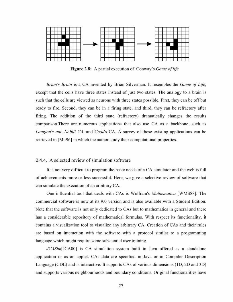
27
Figure 2.8: A partial execution of Conway’s Game of life
Brian's Brain is a CA invented by Brian Silverman. It resembles the Game of Life,
except that the cells have three states instead of just two states. The analogy to a brain is
such that the cells are viewed as neurons with three states possible. First, they can be off but
ready to fire. Second, they can be in a firing state, and third, they can be refractory after
firing. The addition of the third state (refractory) dramatically changes the results
comparison.There are numerous applications that also use CA as a backbone, such as
Langton's ant, Nobili CA, and Codd's CA. A survey of these existing applications can be
retrieved in [Mit96] in which the author study their computational properties.
2.4.4. A selected review of simulation software
It is not very difficult to program the basic needs of a CA simulator and the web is full
of achievements more or less successful. Here, we give a selective review of software that
can simulate the execution of an arbitrary CA.
One influential tool that deals with CAs is Wolfram's Mathematica [WMS88]. The
commercial software is now at its 9.0 version and is also available with a Student Edition.
Note that the software is not only dedicated to CAs but to mathematics in general and there
has a considerable repository of mathematical formulas. With respect its functionality, it
contains a visualization tool to visualize any arbitrary CA. Creation of CAs and their rules
are based on interaction with the software with a protocol similar to a programming
language which might require some substantial user training.
JCASim[JCA00] is CA simulation system built in Java offered as a standalone
application or as an applet. CAs data are specified in Java or in Compiler Description
Language (CDL) and is interactive. It supports CAs of various dimensions (1D, 2D and 3D)
and supports various neighbourhoods and boundary conditions. Original functionalities have

28
been based on the book "Simulation with CA" of J. R. Weimar published in 1998 and
updated in 2002.
MCell [Mce99] was built in the late 90's by Wojtowicz. It offers simulation
functionalities and a rich gallery of 300+ automata rules. Deployed as a Java applet or as a
desktop application, it is open for extensions in which Programmers can add new rules by
programming external Dlls.
Golly [Gol00] is an open source application that was originally built to explore
Conway’s game of life. It has received at least the contribution of several programmers and
therefore contains a vast range of functionality. It can support up to 256 states and has most
known CA in its libraries. One special functionality is its ability to plug in new rules from a
rule table and a rule Tree algorithm. It also has advanced images handling as it can read
common graphic formats (bmp, gif, tiff). It also possesses clipboard functionality for some
copy/pasting functionality.
The web abounds much more simulation Cellular Automaton software than the ones
listed in this section. Each software has its own scheme to present the simulation and often
contains some functionality connected to a specific need of the author. Among others,
FiatLux [Fia01] of Nazim Fates contains functionality from his research on the robustness
of models whose aim is to study the synchronicity in the cell as well as the study of the grid
topology. In this same line of thought, John Walker and Rudy Rucker have created CelLab
[Cel88] for their experimentations related to graphics and design, and originally to
complement functionalities required by the popular Autocad software, a computer-aided
design (CAD / CAM) graphics program. The software mainly deals with 2D CAs and allows
the user to explore it. Each user can design his own rule by writing short programs in Java
and see the evolution on the screen. It contains considerable amount of functionalities
including its ability to simulate heat flow, diffusion of gases, annealing of metal, chemical
reactions and eco systems of artificial life, which have contributed to its popularity and often
used as backbones of others simulation software.

29
Chapter 3
3. The Model
In this chapter, we are introducing the model used in our research. We start by enunciating a
formal definition of a Cellular Automaton which we have briefly introduced in Chapter 1 as
a cellular space where cells change their state synchronously according to local rules. Then,
we present the concise mapping from the network decontamination problem into the concept
of a CA execution. We introduce two new concepts that complement the standard CA
model: Visibility Hop and Contamination Distance. We give the impact of these two new
notions on the two ubiquitous von Neumann and Moore neighbourhood. Then, we present
the various assumptions considered in this thesis including the contamination model and the
immunity model. We conclude the chapter by enunciating the notation used in the
upcoming chapters, including a new visual notation of transition rules that intends to bring
more clarity to the understanding of the rule's objective.
3.1. The Cellular Automaton model
Let us formally define a Cellular Automaton and its properties:
Definition 3.1. Formally, a Cellular Automaton is a quadruple ),,,( fNSZ dwhere
- d is its dimension so dZ is its discrete space of dimension d;
- S is a finite set whose elements are the cell states;
- dZN is its neighbourhood;
- SSf n : is its local transition rule where n is the neighbourhood size.
Definition 3.2. A configuration SZc dt : is the attribution of a state to each cell of the
CA at a specific time t.
3.1.1. 2D CA as State space
Induced from Definition 3.1., a two-dimension Cellular Automaton, simply
abbreviated by 2D CA, is described by a quadruple ),,,( 2 fNSZ .

30
The future state of any cell x at time t+1 is generally induced by the state of the cells
surrounding it at the previous time t. Formally, )(xS at time 1t is defined by a function
on )(xN at time t. The composition of )(xN (and therefore its cardinality) relies on the cells
which are visible to x . The use of a CA for solving the problem of decontamination of a
network is motivated by two simple facts. First, the possible states of nodes in the network
are represented by the transition states of the CA. Second, the algorithm for the Network
Decontamination is defined by the collection of transition rules of the CA.
3.1.2. Network Host state as Transition State
In Network Decontamination using CAs, the state space of the CA has three states:
Contaminated, Decontaminating and Decontaminated, respectively denoted in the current
literature as 1 , and 0. Thus, },1,0{ S .
A host in the network that is infected by a virus is represented by a CA cell which is in
the contaminated state. When the antivirus program is executed on the host, the cell is in a
decontaminating state. When the antiviral program has been successfully executed, the CA is
in a decontaminated state. The hypothesis is that every cell is considered Contaminated and
the goal is to reach a state where all cells are simultaneously in a Decontaminated state. At
time t=0, the given initial configuration is altered by the pre-selection of a finite list of cells
that will be chosen to run the decontaminating program (and thus be in a Decontaminating
state). Then, cell states are synchronously updated at each time step by the local transition
rule applied to their neighbourhoods. Each cell is expected to transition from the
contaminated state into decontaminating to be decontaminated and remain as such. A formal
definition of the process is presented in the next subsection.
In our study, we will define a state called absent, which is not a transition state but
rather a neighbouring state that denotes the absence of a neighbour. The neighbouring state
absent has been introduced in our study for computational reasons and the definition is more
meaningful when a cell within the grid can have its neighbour removed from the topology
for investigation purposes. We mainly use the absent state when we investigate the
removal/addition of a cell inside the CA that can affect the minimum number of
decontaminating cells needed. This feature is implemented in our CA editor and simulator
for network decontamination, as discussed in Chapter 7. However, the introduction of this

31
new state brings certain dilemmas to the state of the neighbouring cells that lie on the border
of the CA. To be consistent with the definition, a cell on the border of the automata can see
its outer neighbour as absent or decontaminated, the latter being the standard used in current
literature. For instance, consider the top-left cell of a CA under the von Neumann
neighbourhood, which does not have a left neighbour or a top neighbour. In current
literature, the absent neighbour of cells on the border of the CA is considered a
"decontaminated" cell, therefore, the cell sees both of its left and top neighbours as being in
a "decontaminated" state rather than "absent" according to our definition. To solve the
matter, unless it is explicitly specified, our effort will be focused first on the search for
decontamination algorithms that do not differentiate the neighbouring state absent from the
transition state decontaminated.
Regarding the terms used in the remainder of the thesis, we will use the term dirty and
contaminated interchangeably to denote that the host is contaminated. We will also use the
word clean to denote that the cell is in a decontaminated state.
3.1.3. Decontamination algorithms as Cellular Automaton Transition Rules
In Network Decontamination using a 2D CA, the configuration C is then the resulting
map },1,0{: 2 tc at any time t.
At time t=0 of the process, every cell is considered "contaminated". The goal is to
reach a state where all cells are simultaneously in a "decontaminated" state. Formally, given
an initial configuration 0c , that is a map },1,0{: 20 c , cell states are synchronously
updated at each time step by the local transition rule applied to their neighbourhood. Let t
jix ,
denote the state of cell ),( ji at time t, and ),( jiN tthe states of the neighbouring cells of
),( ji . In the case of a von Neumann neighbourhood, ),( jiN t= t
ji
t
ji
t
ji
t
ji xxxx 1,,11,,1 ,,, and
the system behaviour can be described as follows:
1. )),((1
, jiNfx tt
ji
2. If )1()1()1()1( 1,,11,,1
t
ji
t
ji
t
ji
t
ji xxxx then 11
, t
jix
The first point indicates the general law of a state change by following the local rule of
the CA. The second point states that a node becomes contaminated if just one of the
neighbouring cells is contaminated.

32
3.1.4. Conflicting rules and Non-determinism
In deterministic Cellular Automata, the update rules have no probabilistic component:
for a given neighbourhood configuration, the updated cell state is always the same. In this
thesis, only deterministic transition rules are considered and designed. Moreover, rules that
conflicts are forbidden: two or several rules are in conflict when the updated cell state is
different for the same neighbourhood configuration. That is, the previously defined
SSf n : has to be a function.
3.2. New dimensions to the definition of a Cellular Automaton radius
Definition 3.3 The radius r of a 2D CA is a positive integer )( *Nr that designates the
maximum distance between a cell and its neighbouring cells.
The von Neumann neighbourhood
when r=2
b
a x c
d
The Moore neighbourhood
when r=2
b c d
a x e
h g f
Figure 3.1: A representation of the von Neumann and Moore neighbourhood when the
radius distance is equal to 2.
The Figure 3.1 highlights the neighbourhood of a cell under the von Neumann and
Moore neighbourhood when r=2. The original neighbours located at r=1 are the ones having
a label. New neighbours located at r=2 are highlighted in a dark gray background. These
new neighbours are constructed recursively according to the definition of the original
neighbourhood.

33
3.2.1. The Visibility Hop Vh
Definition 3.4 In a finite 2D CA consisting of a model of neighbourhood N, the Visibility
Hop Vh )( *NVh is a concept in which a cell “can see” the state of a neighbour if and only
if the neighbouring cell is located within a radius Vhr .
In general, the current cell only “sees” the state of its direct neighbours which are
located at radius 1. In our study, we will use the von Neumann and Moore neighbourhood
schemes as a base on which to introduce this new metric. Of course, the concept of “seeing”
the state of a larger surrounding induces that these states can now be inserted into transition
rules. Our goal is to add this new dimension to the concept of neighbourhood in order to
find new strategies of decontamination and to improve computational results with respect to
some complexity measures that we introduce in upcoming sections of this chapter. The idea
is to allow the current cell to have more knowledge about its surrounding neighbourhood of
a predefined fixed radius distance denoted Visibility Hop at time t. We believe that that this
knowledge can be used to make better decisions about what transition state the current cell
needs to achieve at time t+1. Greater visibility is easily constructed by simple recursive
transitivity of the neighbourhood at each cell with respect to Vh=1, that is, the cell sees its
direct neighbour and the neighbours of each neighbour recursively.
Our goals are to investigate this new metric with respect to some existing
decontamination algorithms and to develop new heuristics under this new scheme. One will
note that the original von Neumann and Moore neighbourhoods can be seen as having a
Visibility Hop distance equal to 1.
3.2.2. The Contamination Distance Cd
Definition 3.5 In a finite 2D CA consisting of a model of neighbourhood N, the
Contamination Distance Cd is a positive integer )( *NCd in which a clean cell gets
contaminated at time t+1 if it was located at radius Cdr of a contaminated cell at time t.
Generally, if a cell x is decontaminated at time t but is in direct contact with a
contaminated cell y, then x will also be contaminated at time t+1. In [LPS06], a slight
variation has been introduced where the cell only gets contaminated if the majority of its
direct neighbours are contaminated. In both cases, it is worth mentioning that only direct
34
neighbours are considered to be a factor of re-contamination. Here in our research, like the
Visibility Hop, we also point out the existence of a Contamination Distance in which a cell
can be contaminated if its neighbour (at a radius distance d greater than 1) is contaminated.
3.2.3. Relationship between Vh and Cd
Existing links
New links
Original neighbours
New neighbours
Figure 3.2: New edges inserted resulting to a new graph topology when Vh=2 under the
von Neumann neighbourhood.
A greater visibility in the neighborhood could imply two things. First, if we assume
that the central node can consult directly the state of the neighbours which are in a distant
radius r>1, then this implies that a physical network connection exists between the central
node and its new neighbours. Therefore, this implies that the CA no longer represents a
normal grid but rather a new and denser network in which a cell can have more connections
as stated by Figure 3.2. Thus, we face a new network topology. Secondly however, another
hypothesis is that the network topology still is a grid but that greater visibility just insinuate
that the central node possibly have knowledge of the state of its distant neighbors by the
intermediary of nearest neighbors from successive and transitive communication. A direct
consequence is that a step of decontamination becomes equivalent of a series of steps that
are required for each cell to gather the states of all its distant neighbours. We note however
that this situation can pose a problem because there is no genuine guarantee that the
information that reaches the central node is not erroneous since the intermediate nodes might
be contaminated and alter the data that they receive. Indeed, it is a very realistic assumption
that some contaminated nodes may choose to taint the information, manner similar to
Byzantine faults in a distributed network. Consequently, if this second case holds, our

35
assumption is that communicated data within the network are not altered even if they are
originated from contaminated sites.
The addition of Vh and Cd also bring new dynamics to the decontamination process:
Case CdVh . This is the basic decontamination process in which there is no distinction
between the definition of Vh, Cd and the radius r. A node sees a neighborhood of radius
r, but can also be contaminated by these same neighbors.
Case CdVh . Even if every node has a larger visibility, only a specific set of nodes
located in the surrounding area can only contaminate the central node.
Case CdVh . This is a stronger condition because even if a node sees just a smaller
locality of neighborhood, they may still be contaminated by further distant nodes. Note
that even under this case, we present in future Chapters that finding decontamination
algorithms is still feasible.
3.3. Recontamination and Immunity model
3.3.1. The contamination model
Viruses and faults are usually spread within the network environment from an infected
site to a neighbouring site. This process known as network contamination typically depends
on the behaviour of the infected site. In the full-spread contamination model, a clean cell can
be contaminated or re-contaminated at time t as soon as a single neighbour is contaminated
at time t-1. This is also referred to in some literature as contamination by contact. Obviously,
this assumption rule is a key factor in the complexity of the decontamination problem, and
plays an important role in finding a good decontamination strategy. The full-spread
contamination model has been used in [FHL08], [LP09], [BFFS02] and [FNS05]. On the
other hand, different contamination models exist where the fault propagation is relaxed, such
as in the selective spread model where faults only propagate to sites that are susceptible and
only affect neighbouring nodes that are vulnerable. For instance, in [LPS06] and [KP00], the
node is only vulnerable to contamination if a majority of its neighbors are faulty, or if m or
more of its neighbours are infected, where m ≥ 1 is a threshold parameter of the system
[FLPS13]. These different contamination conditions are called contamination rules. This

36
idea which shows realistic practical assumptions has again been considered by researchers
by Luccio et al in [LPS07]. In this thesis, we consider the full spread contamination model
3.3.2. The re-contamination model
A decontamination strategy is said to be "monotone" if, once a node becomes
decontaminated, it does not become contaminated ever again. In most instances of the
decontamination problem, it is known that optimal monotone strategies exist. In our study,
we focus only on monotone strategies.
3.3.3. The immunity model
The definition of Immunity refers to the condition of a cell being immune from any re-
contamination dictated by the contamination rules. The most natural form of immunity arises
from the converse definition of the contamination rule itself. Like in [LPS06], [LPS07], and
[KP00], the site is immune to contamination only when a minority of its neighbors are
contaminated. We consider two forms of Immunity:
Processing Immunity. It is assumed that a site processing an anti-virus program, in other
words in a decontaminating state, is immune to re-contamination.
Temporal Immunity. Another form of immunity has been introduced by Flocchini et al.
in [FMS08] when authors studied strategies to decontaminate tree networks. A team of
mobile agent is able to decontaminate any contaminated node it visits; once the cleaner
leaves the node, the infected note is immune for t ≥ 0 time units. In [Daa12] and
[DFZ10], Daadaa et al. uses similar time based immunity called temporal immunity that
we denote as It. According to Daadaa et al's definition, a clean cell always remains
"clean" for a predefined time It=t (or a predefined number of steps in a synchronous
system) regardless of the states of its neighbours. The formal definition of the
decontamination process under some Immunity time is taken from [Daa12] (see below)
and complements the formal definition of the decontamination process presented in
previous section. Let t
jis , be the immunity time of a decontaminated cell located at
position ),( ji at time t. Again, taking the von Neumann neighbourhood definition as an
example, the behaviour of the system from time t to time t+1 is described as:

37
1. )),((1
, jiNfx tt
ji
2. a) if 0,
1
, t
ji
t
ji xx . Let Its t
ji ,
b) if 0, t
jis then 11
, Its t
ji .
c) if 0, t
jis and ( )1()1()1()1( 1,,11,,1
t
ji
t
ji
t
ji
t
ji xxxx then 11
, t
jix .
The first point is similar to the case of a normal decontamination process without an
immunity time, that is, the law of a state change following the local rule of the CA. The
second point states the degradation of the decontamination state, that is, the node become
less and less immune to contamination and eventually becomes contaminated if at least one
of its neighbours is contaminated. One will note that a) and b) are the specifications added
from the immunity-free decontamination process formalization.
In this thesis, we first investigate decontamination heuristics within the full-spread
contamination model (a contaminated site will spread its virus to all its neighbors) and in
which the immunity level of a decontaminated cell is nil (a cell is infected as soon as it is in
contact with a contaminated cell). Second, we study a selective spread contamination model
based on temporal immunity (as previously defined). We show that we can produce
interesting decontamination algorithms that combine Time Immunity and the Visibility
Hop/Contamination Distance just introduced in this research.
3.4. Terms and Notations
Throughout the thesis, we consider few abbreviations. The term Cellular Automaton is
often abbreviated as CA and the plural term Cellular Automata as CAs. The Neighbour
Visibility Hop is abbreviated as Vh. The Contamination Distance is abbreviated as Cd. The
Immunity Time is abbreviated as It.

38
3.4.1. Transition state notation and representation in grayscale/color mode
Traditional notation
in current literature
(e.g. for proofs)
Representation in
figures using
Grayscale mode
Representation in
figures using
Color mode
Contaminated 1
Decontaminating
Decontaminated 0
Generic *
Absent N/A x
Table 3.1: Various notations of the transition state of a CA in current literature and in
this thesis.
In this thesis, we intermittently use notation and representation as listed in Table 3.1
depending on its relevancy. The current literature generally uses grayscale mode to represent
transition states. In this thesis, we add a representation of the neighbourhood in colour mode
as these rules are provided by the research tool that we have implemented and presented in
Chapter 7. Therefore, with respect to the various states of a cell in a CA, the following
notations are used in this thesis.
A Contaminated (also referred to as Dirty) state is denoted by the symbol 1 in theoretical
explanations. Within a CA figure and some listings of decontamination rules, it will be
represented by a circle with an empty background in a grayscale mode or a red circle
in a color mode.
A Decontaminated (also referred to as Clean) state is denoted by the symbol 0 in
theoretical explanations. Within a CA figure and some listings of decontamination rules
(see upcoming sections), it will be represented by a circle with a grey background in
grayscale mode or a green circle in a color mode.
A Decontaminating state is denoted by a circle with a black background both in
theoretical explanations and within a grayscale mode figure , but in a blue color in a
color mode.
A generic arbitrary state is denoted by * in theoretical explanations and in grayscale
figures but as an empty circle in color mode.

39
An Absent node is denoted by X in figures in grayscale mode and with a black circle
in color mode.
A summary of these notations is listed in Table 3.1.
3.4.2. New Neighbourhood configuration notation
We reiterate that the Neighbourhood Configuration is denoted by },,,,{ dcbaxN
and },,,,,,,,{ hgfedcbaxN respectively under the von Neumann and Moore
neighbourhoods when Vh=1. We intermittently call it direct neighbourhood.
In this thesis, we introduce a new notation when Vh>1. In the case of basic
decontamination with Vh=1, each transition rule involves only 4 cells in the neighbourhood
configuration under von Neumann neighbourhood and 8 cells under the Moore
neighbourhood. With the introduction of the concept of Vh, the number of transition rules
increases considerably. For instance, when Vh=2, 8 new cells are added to the von Neumann
neighbourhood so each new rule has the possibility to contain up to 12 cells (Figure 3.1). In
the case of the Moore neighbourhood, this addition is lined with 16 new cells and,
consequently, a transition rule can involve up to 24 cells. The situation of substantial growth
in the number of cells within the neighbourhood configuration may lead to confusion when
using the traditional notation, that is,
},...,,,,,{ ldcbaxN under the von Neumann neighbourhood; and
},...,,,,,,,,,{ xhgfedcbaxN for the Moore neighbourhood.
This could confuse the reader in understanding the logic behind the rule itself. This
potential confusion prompted us to introduce a new notation of the configuration of the
neighbourhood whose purpose is mainly to provide greater clarity about the neighbourhood
configuration. This new notation is based on the "visual" configuration of the neighbouring
cells involved within the rules. A sample of this notation is depicted in Figure 3.3. Another
considerable advantage is to give the reader a faster understanding of the dynamics of the
transition rule embedding the neighourhood (e.g. a left-to-right flow or a diagonal flow etc).
We have two variations of the notations: the Grayscale mode and the Color mode. The latter
mode were introduced as we used our research software tool (which we introduce in Chapter
7) to import transition rules.

40
Neighbourhood Grayscale Mode Color Mode
Von Neumann
Moore
**
***
(a)
(b)
(c)
(d)
Figure 3.3: A sample of the new notation of a transition rule using a grayscale or color
visual representation of the neighbourhood.
The grayscale mode also flags the reader by noticing that the configuration follows a
von Neumann representation by having the concerned inner cell surrounded by a cross (see
Figure 3.3a) and in the case of a Moore neighbourhood by a square (see Figure 3.3b). Within
the notation, direct neighbours are always represented. (The neighbours of a visibility of 1
are the ones on the extremity of the cross in Figure 3.3a and the ones lying on the square in
Figure 3.3b). In both notations, the neighbour's state of distance of 2 or greater is only
represented if the state matters. In other words, we only write the cell state of the neighbour
at distance greater than 1 if the state is other than generic, and missing cells can be of any
state. For instance,
Figure 3.3a stipulates that if at time t, the concerned contaminated cell has both of its
left and top neighbours in a decontaminating state and its left and top neighbour of
distance 2 in a decontaminated state then it transits to a decontaminating state at time
t+1.
Figure 3.3b stipulates that the concerned contaminated cell transits into a
decontaminating state at time t+1 if at time t it respects the following conditions: its left
and right neighbours are in a clean state; its bottom neighbour is in a dirty state; and both
of its left and top neighbours of distance 2 in are in a decontaminating state, regardless of
all its three direct top neighbours.

41
The colour mode includes all cells in the neighbourhood in which state obeys the
configuration presented in Table 3.1.
3.5. Complexity measures
Maximum Decontaminating cells and Average Decontaminating cells. The first metric
we will use to judge the optimality of the decontamination algorithm is the maximum
number of decontaminating cells at any given time. The second metric is the average
number of decontaminating cells at each step during the entire decontamination process.
Decontamination time. Since the decontamination is done synchronously among all cells,
the time is expressed by the number of steps or the number of rounds that the cells run
the local rules until the CA is fully decontaminated.
Immunity time. The minimization of the value of the immunity time is also considered.

42
Chapter 4
4. Decontamination with Visibility Hop
and Contamination Distance
In this chapter, we introduce the concepts of Visibility Hop and Contamination Distance by
analyzing their effects on known basic decontamination algorithms. Our goal is to elaborate
what the new concept of Visibility Hop brings to the network decontamination problem. For
instance, we would like to know if changing the visibility of every node will relax or
complicate the decontamination problem, and if so, under what conditions and which
neighbourhood configuration. We look at known basic decontamination strategies for CAs
and the impact of having a greater Visibility Hop. We consider the grid (or mesh) and its
circular version when Vh=1, which is naturally described by a finite 2-dimensional three
state CA. The topology inferred by the the 2-dimensional CA when Vh>1, as presented in
Chapter 3, is also taken in consideration.
4.1. General Concept
Definition 4.1 In a 2D CA, a Surface Block is a set of cells such that:
1. All cells have the same state
2. All cells of the surface block constitute a connected sub-graph of the CA (i.e. they
are contiguous).
Any Network Decontamination strategy without immunity conceptually splits the
network topology in 3 distinctive surface blocks as depicted by the Figure 4.1 :
the block set C which forms the contaminated cells;
the block set D which forms the decontaminated cells; and
the block set T which is a transition set between the contaminated state and the
decontaminated state.

43
0
0
0
00 0
0
0
00
1
1
1
1 1
1
1
1
1
1
1 11
1
1
1
1T: Set of decontaminating cells
C: Set of contaminated cells1
0 D: Set of decontaminated cells
Decontamination flow direction
Figure 4.1: The decontamination block
The execution of the decontamination algorithm itself can be represented by the
evolution of the cardinality of these three distinct sets. At time t=0 in the beginning of the
process, the network configuration is represented by the full set C and both D and T are
empty. At time t=1, when the algorithm starts, a few cells from C are chosen to compose the
first elements of T. These chosen cells, called the initiators, are not arbitrarily but instead
specifically chosen based on the decontamination flow generated by the decontamination
strategy. Initiators are considered an integral part of the decontamination algorithm itself. At
time t=2 and until the end of the process, local transition rules are applied to each cell. Since
we only consider monotone decontamination algorithms, it is expected that the cardinality of
C will decrease, while the cardinality of D will increase. The process ends when both T and
C are empty and the network configuration is represented by the full set D.
According to our assessment criteria for the effectiveness of the algorithm, minimizing
the time of decontamination is equivalent to finding the most efficient way to transit from
the full set C to the full set D through the set T. Also, minimizing the number of
decontaminating cells is similar to minimizing the cardinality of the set T at any time t

44
during the decontamination process. The efficiency of the strategy depends, among other
factors, on:
the decontamination flow;
the ability to find the most efficient cut to propagate the flow;
the choice of initiators that propagate the flow;
the ability to control the size of T within the propagation flow; and
the time taken by the whole decontamination process.
Let ),( EVG be a graph. Let us recall some standard graph definitions. The number
of edges in a path between two vertices defines its length. The distance between two vertices
x and y, denoted ),( yxd is the length of the shortest path between x and y.
The distance between two disjoint sets of vertices A and B, denoted by ),( BAd is defined as
),( BAd = min { ),( yxd : x is in A and y is in B}
A vertex separator S is a collection of vertices, the removal of which would disconnect the
remaining graph. For instance, the set T is a vertex separator. The width of a vertex
separator is defined as ),( BAd -1, where A and B are two disjoint components when we
remove the vertex separator from the graph.
Observation 4.1. During the execution of a decontamination algorithm, at any time t and
without immunity, if C and D then necessarily T .
In other words C and D cannot share the same border when there is no Time
Immunity, otherwise, cells in C will be contaminated by cells in D. This situation will induce
the following observation on the width of T.
Observation 4.2. During the execution of a decontamination algorithm and under the full-
spread contamination rules, at any time t and without immunity, if C and D then
necessarily the width of any block set T is, at least, Cd.
Proof:
If the width of T is less than Cd, then cells in D can be reached by cells of C.

45
There are few more observations that can also be noted. The set T has more
qualifications than a transition set between the contaminated state and the decontaminated
state. Firstly, its key role is to serve as a "Protection" of the cells in D from being
contaminated by cells from C. Secondly, the set T is not necessarily a closed and connected
set only composed of decontaminating cells. Thirdly, the size and width of T can vary during
the decontamination process.
Definition 4.2 In network decontamination CA, a decontamination algorithm is qualified as
“monotone” when the anti-virus is run only once at each node, that is, once a node is
disinfected, we must guarantee that, regardless of its protection level, the node will stay
clean forever.
In Graph Search, LaPaugh [Lap93] has proven that for every graph G, there is always a
monotone search strategy that uses )(Gs searchers.
Corollary 4.1 When the number of decontaminating cells is fixed and constant (that is, the
number does not change at each step of the decontamination), any monotone strategy is
time-optimal.
Proof: Assume the CA has m rows and n columns and the chosen number of
decontaminating cells for each step is c. The disinfection process cannot be accomplished
within a time c
nmt
* otherwise a step of decontamination would have taken less than c
decontaminating cells.
For all upcoming sections of this chapter, we revisit these basic decontamination
algorithms known as the “left-to-right” or “horizontal flow” but under different Visibility
Hop and Contamination Distance assumptions. Our basic question is whether a larger
visibility will lead to better and more efficient strategies than the optimal ones for Vh=1.
Also, we keep the same hypothesis regarding the immunity time being null (It=0). Since all
these algorithms act in a horizontal flow, we only need the von Neumann neighbourhood to

46
achieve optimality. This is due to the fact that the needed neighbours are the ones located on
the left or right of the concerned cell, and using the Moore neighbourhood will not add any
efficiency to these algorithms.
4.2. Basic Visibility Hop Vh=1
4.2.1. Contamination distance Cd=1
In [Daa12], the problem of the case when there is no immunity (i.e., It=0), the
Contamination Distance is 1 (i.e., Cd=1) and the Visibility Hop is 1 (i.e., Vh=1) is studied. It
is proven that optimal basic decontamination can be achieved in a finite two-dimensional CA
under the von Neumann neighbourhood using n simultaneously decontaminating cells. In the
circular version of the CA, 2n simultaneously decontaminating cells are required and the
process is completed in )(nO time. The same results are achieved under the Moore
neighbourhood.
4.2.2. Contamination distance Cd=2
In this subsection, we present a stricter model than is presented in [Daa12]. We
investigate the case when the Contamination Distance is greater than the Visibility Hop, that
is Vh=1 and Cd>1. An execution of the algorithm is elaborated in the upcoming subsection,
followed by the decontamination theorem and the proof.
4.2.2.1. Grid topology
The idea is to place the initial decontaminating cells in the first column (or the first 2
columns) of the CA (see Figure 4.2). At the initial stage, the first 2 columns are set to
decontaminating, and then the decontaminating strategy begins. Decontaminating cells only
become clean if, and only if, they are protected from the 2-hop contaminated neighbouring
cells. Contaminated cells become decontaminating at time t+1 when their left neighbour
cells were decontaminating at time t. Note that during the process, only a single column
becomes decontaminated within a single unit of time. We can earn one unit of time at the
end of the process (from t=4 to t=5 in Figure 4.2) because the last 2 columns can become
simultaneously clean as every cell in the last column does not need to be protected from a
contaminated neighbour on its right. To do so, we can add an extra rule to tackle the

47
configuration of the last decontaminating column. The effect of the local rules is a sequential
decontamination of columns from left to right, where a decontaminated cell is obviously
never in contact with a contaminated one. The CA is then fully decontaminated in n time
units.
t = 0 t = 1 t = 2
t = 3 t = 4 t = 5
Figure 4.2: A sample execution of the left-to-right basic decontamination under the
von Neumann neighbourhood in a finite CA when Vh=1 and Cd=2
Theorem 4.1. Decontamination is achieved in a finite 2D CA of size mn* )( mn under the
von Neumann neighbourhood using a maximum of n2 simultaneously decontaminating cells
when the Visibility Hop is 1, the Contamination Distance is 2 and the immunity time is null.
Decontamination is achieved in at most m units time.
Proof:
To prove that 2n simultaneously decontaminating cells are sufficient, we need to prove that
starting with n or 2n decontaminating cells initially located in the first column, all cells will
become decontaminated by the end of the process, and no cell will be re-contaminated.
Therefore, we need to show that a set of rules that will perform the operation exists. Table
4.1 depicts this set of rules, inspired by the rules listed in Figure 2.2, in which each cell is
analyzed from its location within the CA (if the cell is laying on the left, top, right, or bottom
border or if the cell is an internal one). The first 6 rules denote the transition of a

48
decontaminating cell into a clean cell. Conversely, the last 6 rules denote the transition of a
contaminated cell into a decontaminating one. Note in the rules R7, R8 and R9, these cells
were decontaminating in the previous step but instead of becoming clean, they have to run
the decontaminating process again to avoid being re-contaminated as their neighbours at
distance 2 are still contaminated. Therefore, R7, R8, and R9 are the rules defining the set T.
This is the key strategy to overcome the Contamination Distance greater than 1, implicitly
simulating a temporal immunity of 1 unit of time.
# Configuration Next State Notes
R1 {•,0,0,•,•} 0 clean if right neighbour is decontaminating
R2 {•,0,•,•,•} 0 Current middle-left decontaminating into a clean cell
R3 {•,0,•,•,0} 0 Current bottom-left decontaminating into a clean cell
R4 {•,•,0,0,•} 0 Last top-right cell decontaminating into a clean cell
R5 {•,•,•,0,•} 0 Last middle-right decontaminating into a clean cell
R6 {•,•,•,0,0} 0 Last bottom-right decontaminating into a clean cell
R7 {•,•,0,1,•} •
R8 {•,•,•,1,•} •
R9 {•,•,•,1,0} •
R10 {1,•,0,1,1} •
R11 {1,•,1,1,1} •
R12 {1,•,1,1,0} •
R13 {1,•,0,0,1} • Rightmost contaminated cells into Decontaminating
R14 {1,•,1,0,1} •
R15 {1,•,1,0,0} •
Table 4.1: Rule for Basic decontamination in Finite CA under the von Neumann
neighbourhood when Vh=1 and Cd=2
A simpler list of rules is proposed in Table 4.2 in which the construction of rules is
based on the propagation flow of the decontamination rather than its location within the CA.
The difference between the two methods of constructing these rules is discussed in
upcoming chapters.

49
# Configuration Next
State Notes
R1 {•,0,0,•,•} 0 clean if right neighbour is decontaminating
R2 {•,0,•,•,•} 0 clean if right neighbour is clean (last column on the CA)
R3 {1,•,1,0,0} • Propagation to the right.
Table 4.2: Alternative Rule for Basic decontamination in Finite CA under the von
Neumann neighbourhood when Vh=1 and Cd=2
4.2.2.2. Circular grid topology
An execution of the algorithm is elaborated in this section, followed by the
decontamination rules and the theorem proof.
t = 0 t = 1 t = 2
t = 3 t = 4
Figure 4.3: A sample execution of the left-to-right basic decontamination under the
von Neumann neighbourhood in a circular CA when Vh=1 and Cd=2
The initial decontaminating cells are placed in any four consecutive columns of the CA
and the cells obey the following simple rules.
A decontaminating cell becomes decontaminated at time t+1
o if both of its left and right neighbours are in a decontaminating state at time t, or
o if one of its left or right neighbours is in a decontaminating state and the
neighbour on the other side is in a decontaminated state at time t.
A contaminated cell becomes decontaminating at time t+1 if it is in contact with a
decontaminating state at time t

50
Figure 4.4: The propagation flow of the basic decontamination under the von
Neumann neighbourhood in a circular CA
Theorem 4.2. Decontamination can be achieved in a circular 2D CA of size
mn* )( mn under the von Neumann neighbourhood using 4n simultaneous
decontaminating cells when the Visibility Hop is 1, the Contamination Distance is 2 and the
immunity time is null. Decontamination is achieved in at most 12
m units time.
Proof:
To prove that 4n simultaneous decontaminating cells are sufficient, we need to prove that a
set of rules exists. These transition rules are shown in Table 4.3. At each step, two columns
get decontaminated so the process should be completed in at most units of
2
m time.
However the rule R1 allows the algorithm to save one step at the last stage of the process
since the last four columns (if n is even) or the last three columns (if n is odd) gets
simultaneously decontaminated.

51
# Configuration Next State Notes
R1 {•,•,*,•,*} 0
Clean if both the left & right neighbour is
decontaminating
R2 {•,0,*,•,*} 0 Clean if the left neighbour is clean & right
neighbour is decontaminating
R3 {•,•,*,0, *} 0
Clean if the left neighbour is decontaminating &
right neighbour is clean
R4 {1,•,*,*,*} • Propagation to the left
R5 {1,*,*,•,*} • Propagation to the right
Table 4.3: Rule for Basic decontamination in circular CA under the von Neumann
neighbourhood when Vh=1 and Cd=2
4.3. The impact of a greater Visibility, case study of Vh=2
4.3.1. Contamination Distance Cd=1
4.3.1.1. Grid topology
Similar to the algorithm presented in [Daa12], the process starts by setting the cells of
the first column as initiators. Then, the rules in Table 4.4 can be used to process the
decontamination algorithms. The first observation is that the execution looks identical to the
basic decontamination presented in [Daa12] and having the Vh>1 did not offer any
improvement. Hence, we present the theorem below.
Theorem 4.3. Optimal decontamination is achieved in m unit times, in a finite 2D CA of size
mn* )( mn under the von Neumann neighbourhood using n simultaneous decontaminating
cells when the Visibility Hop is 2, the Contamination Distance is l and the immunity time is
null.
Proof:
The proof presented in [Daa12] shows that any decontamination strategies without immunity
and with Contamination Distance 1 will require at least n simultaneously decontaminating
cells. The same proof works independently of the visibility of every node. Therefore, the
basic strategy presented in [Daa12] is optimal regardless of the visibility of every node.

52
# Configuration Next
State Notes
R1 {•,*,*,*,*} 0 Any decontaminating cell is clean in the next iteration
R2 {1,•,0,1,1} •
R3 {1,•,0,0,1} •
R4 {1,•,1,1,1} •
R5 {1,•,1,1,0} •
R6 {1,•,1,0,1} •
R7 {1,•,1,0,0} •
Table 4.4: Rule for Basic decontamination in Finite CA under the von Neumann
neighbourhood when Vh=2 and Cd=1
4.3.1.2. Circular grid topology
For the circular case, the algorithm execution is exactly similar to the case Vh=1,
Cd=1. The process starts by setting any two consecutive cells as initiators and propagates
the decontamination in opposite directions in the CA (left to right and right to left).
t = 0 t = 1 t = 2
t = 3 t = 4
Figure 4.5: A sample execution of the left-to-right decontamination under the von
Neumann neighbourhood in a circular CA when Vh=2 and Cd=1

53
Theorem 4.4. Optimal decontamination can be achieved in at most
2
m units time in a
circular 2D CA of size mn* )( mn under the von Neumann neighbourhood using 2n
simultaneous decontaminating cells when the Visibility Hop is 2, the Contamination
Distance is 1 and the immunity time is null.
Proof: The same induction proof for optimality for the case Vh=1, Cd=1 in [Daa12] holds
here too, since it works independently of the visibility of every node. The transition rules
of the decontamination are shown in Table 4.5.
# Configuratio
n
Next
State Notes
R1 {•,*,*,*,*} 0
Any decontaminating cell is clean in the next
iteration
R2 {1,*,*,•,*} • Propagation to the left
(decontaminating if right neighbour is
decontaminating)
R3 {1,•,*,*,*} • Propagation to the right
(decontaminating if left neighbour is
decontaminating
Table 4.5: Rule for Basic decontamination in a circular and Finite CA under the von
Neumann neighbourhood when Vh=2 and Cd=1
4.3.2. Contamination Distance Cd=2
4.3.2.1. Grid topology
The algorithm previously presented (Cd=2 and Vh=1) will still behave correctly if
executed against a model of CA with greater visibility (i.e., when Vh>1), both in the case of
a basic 2D mesh or the circular 2D mesh. Thus, the above mentioned examples of execution
of the case Vh=1 and Cd=2 still hold for the case Vh=2 and Cd=2, and the same rules can
still be applied to perform the decontamination. In fact, with a greater visibility, we will
show that better results are achieved with respect to the time execution of the algorithm.
Decontamination is achieved by setting all cells of the first 2 columns to decontaminating

54
and by applying the set of rules indicated in Table 4.6. Figure 4.6 shows the propagation of
decontamination starting with decontaminating cells located in the two left most columns.
Theorem 4.5. Decontamination is achieved in a finite 2D CA of size mn* )( mn under the
von Neumann neighbourhood using 2n simultaneously decontaminating cells when the
Visibility Hop is 2, the Contamination Distance is 2 and the immunity time is null.
Decontamination is achieved in at most
2
m units time.
Proof:
In the case where Vh=1, even if we started the decontamination with the first two columns
on the left, the algorithm would have faced two restrictions. The first restriction is that only a
single column of cells could be decontaminating into the next step. The second restriction is
that only a single column of cells in a decontaminating mode could be decontaminated. The
other column of cells (the right column) would have to remain in a decontaminating state,
otherwise, it would be re-contaminated in the next step as the column would be in contact
with its right neighbour of distance 2. Generally, in any step of decontamination, if columns
k and k+1 are decontaminating at time t, it means that at time t+1, the limitation is that a
single decontaminating column could be decontaminated and only one contaminated column
could be decontaminating. Thus, only the column k could be decontaminated. The column
k+1 must remain in its decontaminating state and cannot be decontaminated, otherwise, it
would be re-contaminated by the k+3 column (because that Cd=2).
The only way that the k+1 column changes its state into decontaminated is if the column
k+3 could also change its state into a decontaminating mode, and therefore could protect the
k+1 column. This is not feasible. It is impossible to find a rule that could change the states of
the cells in column k+3 from contaminated to decontaminating because they are surrounded
left and right by infected cells and the visibility is Vh=1. The column k+3 turns out to be
identical to all remaining contaminated columns of the CA. A rule that would change the
state of the column k+3 will also change the state of its other remaining contaminated cells.
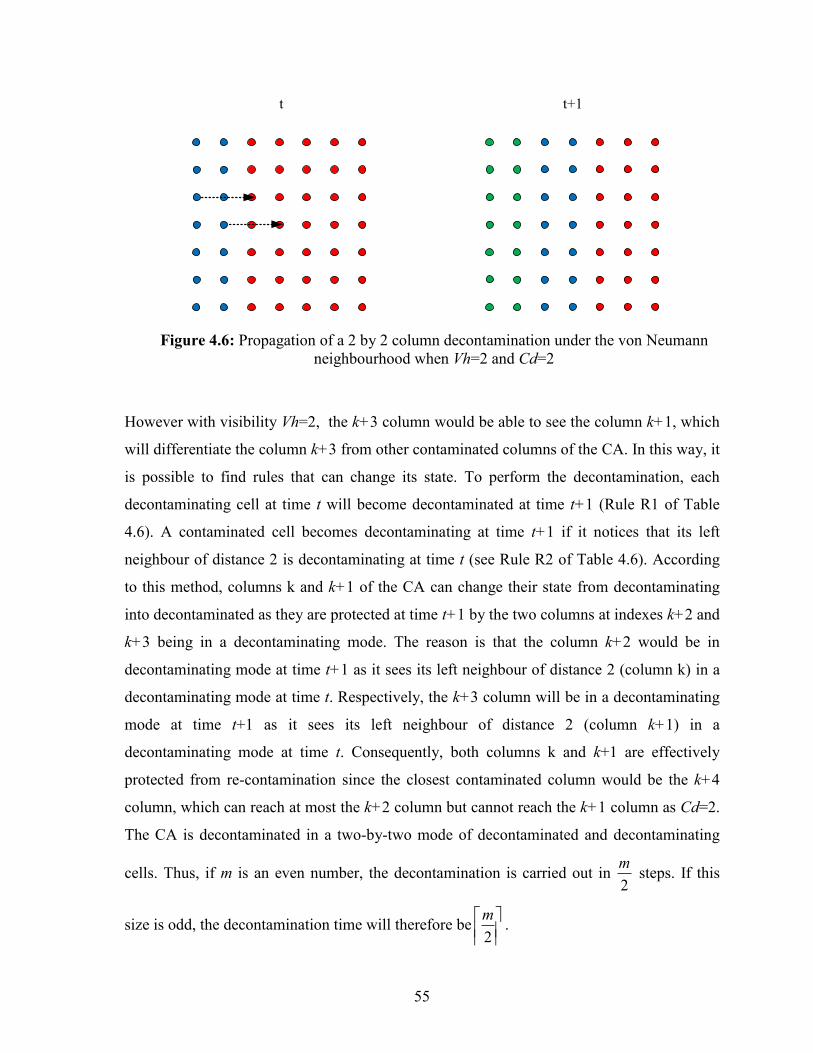
55
t t+1
Figure 4.6: Propagation of a 2 by 2 column decontamination under the von Neumann
neighbourhood when Vh=2 and Cd=2
However with visibility Vh=2, the k+3 column would be able to see the column k+1, which
will differentiate the column k+3 from other contaminated columns of the CA. In this way, it
is possible to find rules that can change its state. To perform the decontamination, each
decontaminating cell at time t will become decontaminated at time t+1 (Rule R1 of Table
4.6). A contaminated cell becomes decontaminating at time t+1 if it notices that its left
neighbour of distance 2 is decontaminating at time t (see Rule R2 of Table 4.6). According
to this method, columns k and k+1 of the CA can change their state from decontaminating
into decontaminated as they are protected at time t+1 by the two columns at indexes k+2 and
k+3 being in a decontaminating mode. The reason is that the column k+2 would be in
decontaminating mode at time t+1 as it sees its left neighbour of distance 2 (column k) in a
decontaminating mode at time t. Respectively, the k+3 column will be in a decontaminating
mode at time t+1 as it sees its left neighbour of distance 2 (column k+1) in a
decontaminating mode at time t. Consequently, both columns k and k+1 are effectively
protected from re-contamination since the closest contaminated column would be the k+4
column, which can reach at most the k+2 column but cannot reach the k+1 column as Cd=2.
The CA is decontaminated in a two-by-two mode of decontaminated and decontaminating
cells. Thus, if m is an even number, the decontamination is carried out in 2
m steps. If this
size is odd, the decontamination time will therefore be
2
m.

56
# Configuration
Next
State Notes
R1
Any decontaminating cell will be
decontaminated in the next step.
R2
*
***
A contaminated cell will be decontaminating
at time t+1 if its left neighbour of distance 2
is decontaminating at time t.
Table 4.6: Rule for Basic Decontamination in Finite CA under the von Neumann
neighbourhood when Vh=2 and Cd=2
4.3.2.2. Circular Grid topology
The initial decontaminating cells are placed in any four consecutive columns of the CA
and the cells obey the following simple rules:
a decontaminating cell becomes decontaminated at time t+1; and
a contaminated cell becomes decontaminating at time t+1 if it is in contact (with respect
to the visibility Vh=2) with a decontaminating state at time t.
.
Theorem 4.6. Decontamination is achieved with a circular CA of size mn* )( mn under
the von Neumann neighbourhood using 4n simultaneous decontaminating cells if the
Visibility Hop is 2, the Contamination Distance is 2 and the immunity time is null.
Decontamination is achieved in at most
4
m units time.
Proof:
The Table 4.7 shows the list of transition rules for the decontamination. Starting with 4
columns of decontaminating cells, the rules R3 and R4 will initiate 4 new columns at each
step. Since the rule R1 will decontaminate each decontaminating cell at each step, it implies

57
that every successive 4 columns will get decontaminated at each step. Therefore, the
decontamination is executed in
4
m units of time.
# Configuration
Next
State Notes
R1
Any decontaminating cell will be
decontaminated in the next step.
R2
*
***
A contaminated cell will be decontaminating
at time t+1 if its left neighbour of distance 2
is decontaminating at time t.
R3 **
*
*
A contaminated cell will be decontaminating
at time t+1 if its right neighbour of distance
2 is decontaminating at time t.
Table 4.7: Rule for Basic Decontamination in Finite CA under the von Neumann
neighbourhood when Vh=2 and Cd=2
4.4. Summary
We started by enunciating the known results of decontaminating a CA under the von
Neumann configuration. The optimal algorithm needs exactly n decontaminating cells and
the required time of execution is linear based on the size of the CA. In the case of a circular
CA, the optimal algorithm needs 2n decontaminating cells and is performed in
approximately half of the time. Then, we have shown that even with a strict model, in which
we increase the Contamination Distance to Cd=2, it is still possible to execute the
decontamination with a visibility Vh=1. In that configuration, the algorithm needs at least 2n
decontaminating cells with a normal CA and n time units of execution. Thanks to the use of
Visibility Hop, it is possible to decrease the execution time. A summary of results established
in this chapter is listed in the following table.

58
Neighbourhood
Type Topology Vh Cd
Number
of
Initiators
Maximum
decontaminating
cells
Time Reference
von Neumann CA 1 1 n n m [Daa12]
von Neumann Circular
CA 1 1 n n2
2
m [Daa12]
von Neumann CA 1 2 n n2 m
Theorem 4.1 n2 n2 1m
von Neumann Circular
CA 1 2
n2 n4
2
m
Theorem 4.2
3n or n4 n4 12
m
von Neumann CA 2 1 n n m Theorem 4.3
von Neumann Circular
CA 2 1 n2 n2
At most
2
m
Theorem 4.4
von Neumann CA 2 2 n2 n2
2
m Theorem 4.5
von Neumann Circular
CA 2 2 n4 n4
4
m Theorem 4.6
Table 4.8: Summary of the basic decontamination results for a n*m )( mn CA under
the topology, Visibility Hop and Contamination Distance parameters.
In this chapter, we only concentrated on the von Neumann neighbourhood because all
transition rules can be expressed with its cells, and because using the Moore neighbourhood
would not increase the efficiency of these algorithms. We also analyzed the horizontal flow
algorithm with specific values of Vh and Cd. We could have generalized the same algorithm
for different values of Cd and Vh, however, this generalization will be introduced and
studied in the next chapter. To avoid repeating the same ideas, we decided to introduce the
generalization for more sophisticated algorithm.

59
Chapter 5
5. Diagonal Flow
In previous chapters, we focused on either the horizontal or the vertical cuts of our CA. The
flow of decontamination was performed in a vertical way. In this chapter, we focus on a new
way to cut the CA. Rather than doing it in a vertical (column by column) or horizontal (line
by line), the decontamination is still in a straight line but following a diagonal pattern.
5.1. Motivation
In the previous chapter, we noted that decontamination was performed according to a
horizontal flow. The success of this algorithm rests on the basic fact that the
decontamination flow is cutting the CA in a vertical manner from both opposite borders of
the CA. Cutting the CA following a straight line always guarantees the protection of cells
already decontaminated. Moreover, a crucial condition is that the number of
decontaminating cells is always bound to a constant number. Consider Figure 5.1. If a
strategy offers a flow of decontamination from an internal cell, it is very likely that the same
strategy will have some difficulty minimizing the size of T cells because its cardinality will
increase over time. It is trivial that as the size of the square (in Figure 5.1a) or rhombus
(Figure 5.1b) increases, it is necessary to increase the number of decontaminating cells that
are required to protect already cleaned cells. The idea behind the decontamination using
diagonal flow is based on the same motivation as the vertical flow.

60
t=0 t=1 t=2
(a)
(b)
Moore
Von
Neumann
Figure 5.1: A basic propagation of a decontamination approach initiated by an inner cell
showing a bound-less number of decontaminating cells
We also see in the previous chapter that one of the consequences of the sequential
decontamination in a vertical mode is that the block set of decontaminating cells T must
absolutely contain, at a minimum, all the cells within the same column and as many columns
as the value of Cd. However, when using diagonal flow, we will show in the upcoming
sections that it is possible to use less than n decontaminating cells for some steps. We are
also interested in the diagonal approach as it presents a base for a “divide and conquer”
strategy that we will investigate in detail in the upcoming chapters.
5.2. Basic Case of Visibility Vh=1
In this section, we show that with a visibility of 1, it is possible to find some
decontamination algorithms using a diagonal flow under the von Neumann neighbourhood
configuration.

61
t=0 t=1 t=2 t=3
Figure 5.2: Propagation of the basic diagonal move under the von Neumann
neighbourhood when Vh=1 and Cd=1
5.2.1. Contamination Distance Cd=1
The idea is to initiate the algorithm from a cell located on a corner of our CA (Figure
5.2). This chosen cell can be from any corner, but in our example, the selected cell is the one
located on the first column and the first row (top left corner of our CA). Each cell becomes
decontaminated at time t+1 after being in a decontaminating state at time t. The intention of
the algorithm is to create a diagonal decontamination flow from the top-left cell to the
bottom-right cell. In the next step, at time t=2, the algorithm is run by propagating
decontaminating cells in the direction of the diagonal, which in our case is the two neighbour
cells of the initial cell. The process continues to eventually reach the full diagonal (here t=4)
and then a reverse symmetric execution happens until reaching the full decontamination.
With this pattern, the CA will be properly decontaminated. We formulate the following
theorem:
Theorem 5.1. Decontamination using diagonal flow can be achieved with a CA of size
mn* )( mn under the von Neumann neighbourhood if the Visibility Hop Vh =1 and the
Contamination Distance Cd=1 by using at most n decontaminating cells at any time t. The
decontamination process is performed using (m+n-1) steps.
Proof:
To prove that at most n simultaneously decontaminating cells are sufficient, we need to
prove that starting with 1 decontaminating cell initially located in the left corner, all cells
will become decontaminated by the end of the process, and no cell will be re-contaminated.
That is, that once decontaminated, every cells stays decontaminated until the end of the

62
process, when all cells are decontaminated. Therefore, we need to show that such a set of
rules that will perform the operation exists. Table 5.1 lists the needed rules to perform the
decontamination.
# Configuration
Next
State Notes
R1
Any decontaminating cell will be
decontaminated in the next step.
R2
**
Cell located on the top horizontal border of
the CA
R3
**
Cell located on the left vertical border of the
CA
R4
**
Internal Cell
Cell laying on the Right vertical border
Cell laying on the bottom horizontal border
Table 5.1: Rules for decontamination in Finite CA using basic diagonal move under the
von Neumann neighbourhood when Vh=1 and Cd=1

63
5.2.2. Generalization of an arbitrary distance Cd=k
(a)
t=1
(c)
t=n-1(d)
t=2n-k-1
k
k
k
k
k
k
(b)
t=2
k
k
Figure 5.3: Propagation of the basic diagonal move under the von Neumann
neighbourhood when Vh=1 and Cd=k
A generalization of the diagonal strategy under the von Neumann neighbourhood at
various times during the decontamination process, when Vh=1 and for an arbitrary Cd, is
depicted in Figure 5.3. We note that during the entire process, Cd is always equal to k and
only a single diagonal gets decontaminated at each step.

64
Similar to the case of Cd=1, the idea is to initiate the algorithm from a group of cells
located in a corner of our CA (Figure 5.3a). These chosen cells can be from any corner, but
in our strategy, selected cells are the triangle of cells delimited by the first k columns and k
rows (top left corner of our CA). The intention of the algorithm is to create a diagonal
decontamination flow from the top-left cell to bottom-right cell by propagating
decontaminating cells in the direction of the diagonal. At time t=2, only the top-left cell gets
decontaminated and the next diagonal containing the border cell k+1 becomes
decontaminating (Figure 5.3b). The process continues to eventually reach the full diagonal
and then a reverse symmetric execution happens until full decontamination is reached. With
this pattern, the CA will be properly decontaminated.
Beforehand, let us computes the size ),( mnDk of the first k diagonals in a
mn* rectangular grid with the hypothesis that )( mn .
Lemma 5.1. Let ),( mnDk be the size of the first k diagonals in a mn* rectangle grid
)( mn . Since there are 1mn diagonals in the grid, then obviously 1 nmk .
Thus,
),( mnDk =2
)1( kk if nk
),( mnDk = nnknn
)(2
)1(
if mkn
),( mnDk =
nnknn
)(2
)1(
mk
i
in1
)( if 1 nmkm
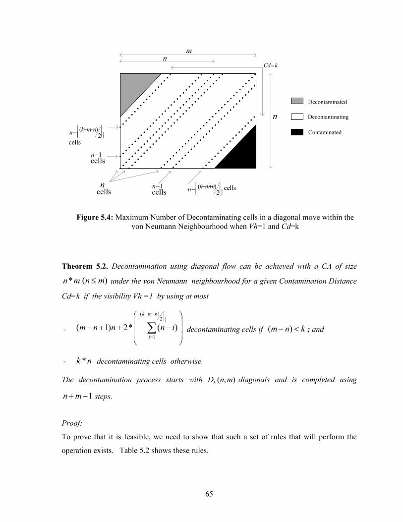
65
Decontaminated
Decontaminating
Contaminated
cells1nn
cells
m
n
n
2
)( nmkn cells
2
)( nmkn
cells
cells1n
kCd
Figure 5.4: Maximum Number of Decontaminating cells in a diagonal move within the
von Neumann Neighbourhood when Vh=1 and Cd=k
Theorem 5.2. Decontamination using diagonal flow can be achieved with a CA of size
mn* )( mn under the von Neumann neighbourhood for a given Contamination Distance
Cd=k if the visibility Vh =1 by using at most
-
2)(
1
)(*2)1(
nmk
i
innnm decontaminating cells if knm )( ; and
- nk * decontaminating cells otherwise.
The decontamination process starts with ),( mnDk diagonals and is completed using
1mn steps.
Proof:
To prove that it is feasible, we need to show that such a set of rules that will perform the
operation exists. Table 5.2 shows these rules.

66
Figure 5.4 shows why at most
2)(
1
)(*2)1(
nmk
i
innnm decontaminating cells are
required when knm )( . It is easy to see that if )( nmkCd then k consecutive
diagonals of size n are needed. It is too simply the maximum size of k consecutive
diagonals in a mn* )( mn rectangular grid. Also since each diagonal gets
decontaminated one at a time, 1mn steps are required to perform the operation since
there are 1)()12( mnnmn diagonals of the CA being involved.
# Configuration
Next
State Notes
R1
k
k
R2
k
Cell laying on the vertical right border
(including top right corner but excluding
bottom right corner)
R3
k
Cell laying on the bottom border
(including bottom left corner but excluding
bottom right corner)
Last cell during decontamination (Bottom

67
R4
Right corner)
R5
**
Cell located on the top horizontal border of
the CA
R6
**
Cell located on the left vertical border of the
CA
R7
**
Internal Cell
Cell laying on the Right vertical border
Cell laying on the bottom horizontal border
Table 5.2: Rules for Basic Decontamination in Finite CA using diagonal move under the
von Neumann neighbourhood when Vh=1 and for an arbitrary Cd=k
5.3. The impact of a greater Visibility ( 2Vh ) on Diagonal Moves
In this section, we show that with a visibility 2Vh , it is possible to improve the
execution time of the strategy using a diagonal flow under the von Neumann neighbourhood
configuration.
5.3.1. Contamination Distance Cd=1
The decontamination rules for Cd=1 and Vh=1 (Table 5.1) also hold when Vh=2 and
the process is even identical for a visibility 2Vh . Since we still want to minimize the
number of decontaminating cells, only a single decontaminating diagonal is sufficient at
each step even if more diagonals can be processed because of a greater visibility.
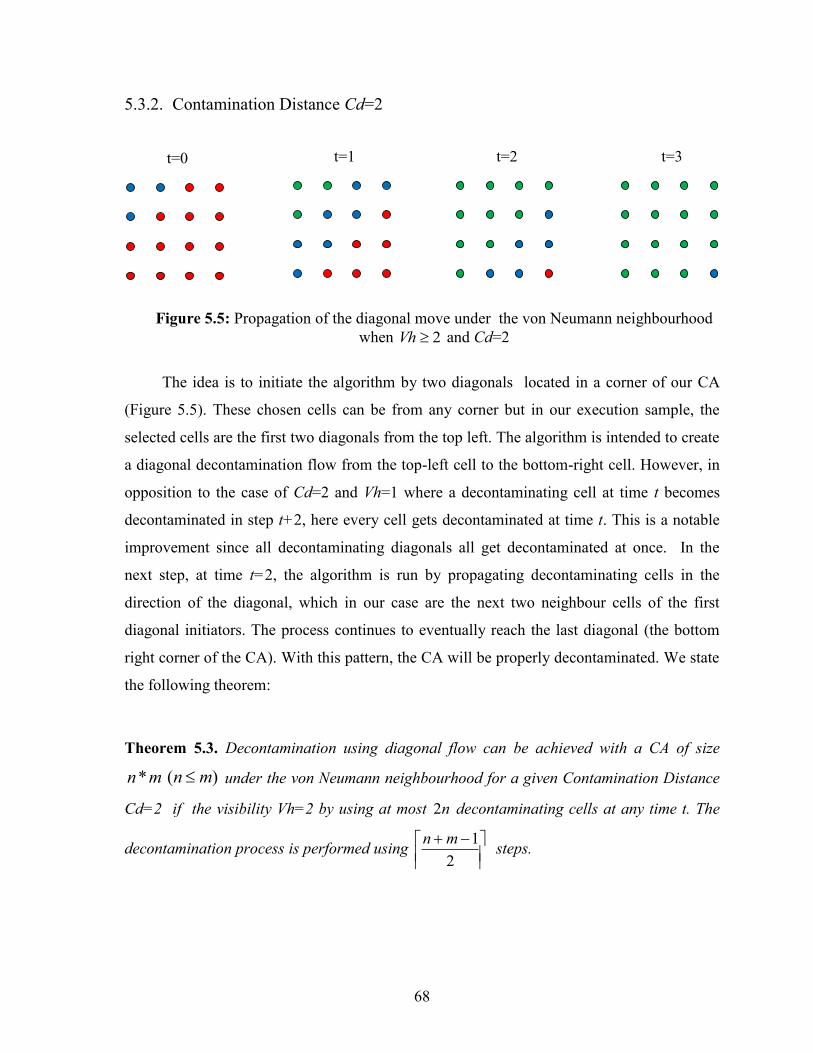
68
5.3.2. Contamination Distance Cd=2
t=0 t=1 t=2 t=3
Figure 5.5: Propagation of the diagonal move under the von Neumann neighbourhood
when 2Vh and Cd=2
The idea is to initiate the algorithm by two diagonals located in a corner of our CA
(Figure 5.5). These chosen cells can be from any corner but in our execution sample, the
selected cells are the first two diagonals from the top left. The algorithm is intended to create
a diagonal decontamination flow from the top-left cell to the bottom-right cell. However, in
opposition to the case of Cd=2 and Vh=1 where a decontaminating cell at time t becomes
decontaminated in step t+2, here every cell gets decontaminated at time t. This is a notable
improvement since all decontaminating diagonals all get decontaminated at once. In the
next step, at time t=2, the algorithm is run by propagating decontaminating cells in the
direction of the diagonal, which in our case are the next two neighbour cells of the first
diagonal initiators. The process continues to eventually reach the last diagonal (the bottom
right corner of the CA). With this pattern, the CA will be properly decontaminated. We state
the following theorem:
Theorem 5.3. Decontamination using diagonal flow can be achieved with a CA of size
mn* )( mn under the von Neumann neighbourhood for a given Contamination Distance
Cd=2 if the visibility Vh=2 by using at most n2 decontaminating cells at any time t. The
decontamination process is performed using
2
1mn steps.

69
Proof:
To prove that it is feasible, we need to show that such a set of rules that will perform the
operation exists. Table 5.2 and Table 5.4 show two alternatives. Since at most two
diagonals can be in a decontaminating state, the cardinality of T is at most n2 which the
maximum size of two consecutive diagonals. Note that for a square CA (that is, nm ), at
most 12)1( nnn decontaminating cells are required. With respect to the
decontamination time, two diagonals get decontaminated at each step (except perhaps the
last diagonal represented by a single cell). Since there are 1)()12( mnnmn
diagonals, the decontamination time is
2
1mn steps.

70
# Configuration
Next
State Notes
R1
Any decontaminating cell will be
decontaminated in the next step.
R2
**
Cell laying on the vertical left border
R3
**
Cell laying on the horizontal top border
R4
**
*
*
Internal cell
Cell laying on the vertical right border
Cell laying on the horizontal bottom border
Table 5.3: Rules for Basic Decontamination in Finite CA using diagonal move under the
von Neumann neighbourhood when Vh=2 and Cd=2
A more simplistic rule is proposed in Table 5.4. We note that there are some situations
where some cell’s transition states can be eligible through both R2 and R3, but in these
cases, the automata is still deterministic since the resulting state (decontaminating) is
identical.

71
# Configuration
Next
State Notes
R1
Any decontaminating cell will be
decontaminated in the next step.
R2
**
* *
R3
***
*
R4
*
*
Only to trigger the decontamination for the
cell located on the second line & second
column
Table 5.4: Another possible set of rules for Basic Decontamination in Finite CA using
diagonal move under the von Neumann neighbourhood when Vh=2 and Cd=2

72
5.4. Generalization for an arbitrary Cd and Vh
(a)
k
k k
k
(b)
k
k
k
k
k
k
(c)
Figure 5.6: Propagation of the diagonal move under the von Neumann neighbourhood
when Vh=Cd=k
In an attempt to generalize the diagonal strategy for any given Cd=k and any arbitrary
Vh=j, we first look at the case of k=j and let us use Figure 5.3 as a reference. Because Cd=k,
we first note that during the entire process, the width of the set of decontaminating cells T is
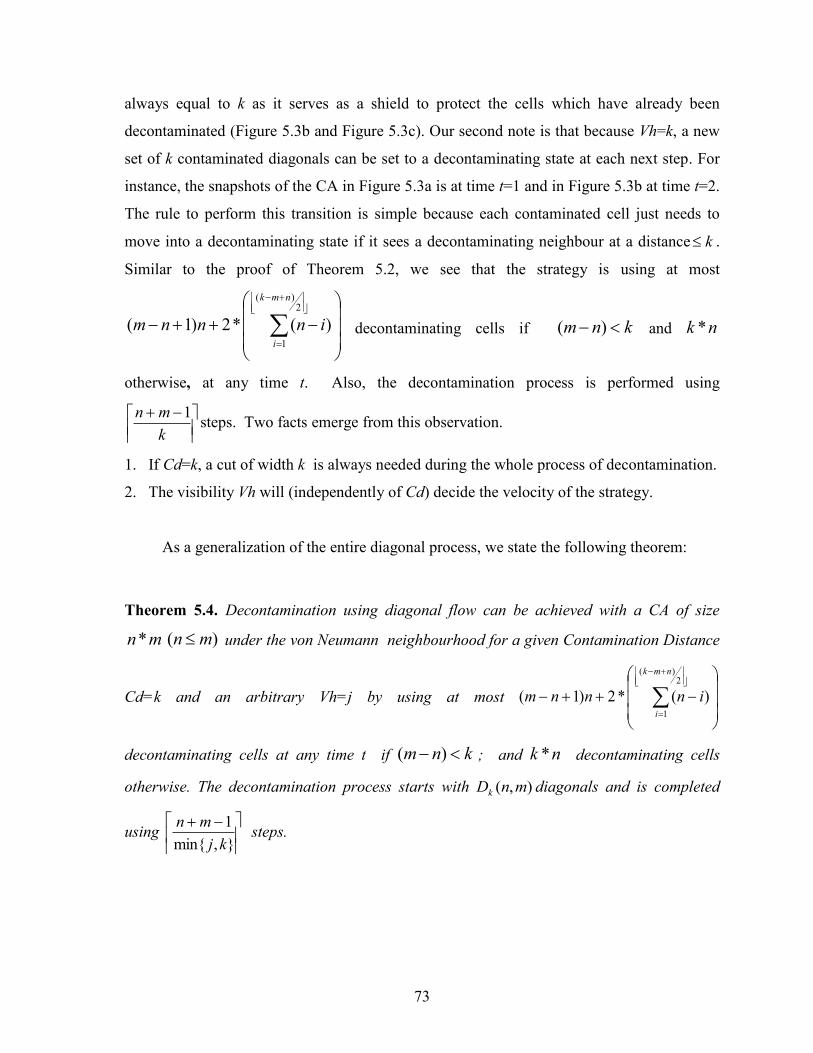
73
always equal to k as it serves as a shield to protect the cells which have already been
decontaminated (Figure 5.3b and Figure 5.3c). Our second note is that because Vh=k, a new
set of k contaminated diagonals can be set to a decontaminating state at each next step. For
instance, the snapshots of the CA in Figure 5.3a is at time t=1 and in Figure 5.3b at time t=2.
The rule to perform this transition is simple because each contaminated cell just needs to
move into a decontaminating state if it sees a decontaminating neighbour at a distance k .
Similar to the proof of Theorem 5.2, we see that the strategy is using at most
2)(
1
)(*2)1(
nmk
i
innnm decontaminating cells if knm )( and nk *
otherwise, at any time t. Also, the decontamination process is performed using
k
mn 1steps. Two facts emerge from this observation.
1. If Cd=k, a cut of width k is always needed during the whole process of decontamination.
2. The visibility Vh will (independently of Cd) decide the velocity of the strategy.
As a generalization of the entire diagonal process, we state the following theorem:
Theorem 5.4. Decontamination using diagonal flow can be achieved with a CA of size
mn* )( mn under the von Neumann neighbourhood for a given Contamination Distance
Cd=k and an arbitrary Vh=j by using at most
2)(
1
)(*2)1(
nmk
i
innnm
decontaminating cells at any time t if knm )( ; and nk * decontaminating cells
otherwise. The decontamination process starts with ),( mnDk diagonals and is completed
using
},min{
1
kj
mn steps.

74
Proof:
Without loss of generality, we assume mn and we start the process from the top left corner
of the CA. To simplify the proof, we assume the CA is rotated in such a way that the vertical
border height is n and the horizontal border width is m.
The process starts by choosing ),( mnDk initiators which are composed by the first k
diagonals from the top left corner, note T. At each iteration, the set T is recreated by three
rules
1. A subset of T, say D, composed by the first j diagonals from the top left (that is, a cut of
width j) is removed from T and gets decontaminated.
2. The remaining set of diagonals, that is DT / of width jk remains in a
decontaminating state and therefore stays in T.
3. The next j contaminated diagonals of the CA located right after T go to a
decontaminating state and these new cells are added to the set T.
With respect to the maximum number of decontaminating cell and the number of initiators,
the proof is identical to the one of Theorem 5.2. which is completed with Lemma 5.1.
When Vh<Cd, the process can only execute Vh=j diagonals at a time. Otherwise, when
Vh>Cd, the process execute a minimum of Cd=k up to a maximum of Vh=j diagonals at a
time. In this case, since we want to minimize the cardinality of T, we choose to process
Cd=k diagonals. Therefore, the execution time of the algorithm is
},min{
1
kj
mn.
5.5. Summary
In this chapter, we studied a new decontamination strategy that is based on a diagonal
flow. Note, that we put the focus on von Neumann neighbourhood because all transition
rules can be expressed with its cells. We also analyzed the diagonal flow algorithm with
specific values of Vh and Cd. We completed the chapter by giving a generalization of the
decontamination strategy using diagonal flow for any arbitrary value of Cd and Vh. A
summary of results established in this chapter is listed in Table 5.5.

75
The Diagonal Move approach is an improvement over the horizontal flow algorithm
presented in Chapter 4 with respect to the average number of decontaminating cells. Take for
instance the special case of the square grid (m=n) during the basic setup of Vh=1 and Cd=1,
the horizontal flow has an average use of nn
n
2
decontaminating cells at each step
compared to only 12
2
n
n decontaminating cells for the diagonal move. With respect to the
general case of an arbitrary Vh and Cd, the horizontal flow always processes a constant
number of k=Cd set of diagonals (in which each diagonal contains n cells) at each step.
Therefore, the average number of decontaminating cells at each step is k*n. However for
the diagonal move, the same k*n decontaminating cells only appears in the
decontamination process
k
nm 1 times. In the rest of the process, the diagonal moves
considerably use less than k*n decontaminating cells.

76
N*
Type Vh Cd
Number
of
Initiators
Max
D*ing
cells
Time Ref.
VN 1 1 1 n n2 Th.
5.1
VN 1 k ),( nmDk
2)(
1
)(*2)1(
nmk
i
innnm if
knm )(
nk * , if knm )(
1mn Th
5.2
VN 2 2 3 n2 , if nm
12 n , if nm
2
1mn
Th
5.3
VN j k ),( nmDk
2)(
1
)(*2)1(
nmk
i
innnm if
knm )(
nk * , if knm )(
},min{
1
kj
mn Th
5.4
Table 5.5: Summary of decontamination results of an n*m (nm) CA using Diagonal
move strategies.

77
Chapter 6
6. Subdividing Strategies
In this chapter, we focus our research on a new approach which consists of investigating
multiple cuts across various locations of the CA,. The idea is relatively similar to the widely
known divide and conquer approach because the aim is to divide a large problem into several
sub-problems and apply the same solution to these partitioned sub-problems. However, in
our case, the base decontamination strategy needs a slight modification when applied to the
various subdivisions. We show in every case that the base algorithm will always require
some update in order to work on the divided substructure. Our goals are to show that we can
perform such a strategy (the basic algorithm and the subdivision) and show that the
Visibility Hop and Time immunity become important factors with respect to the feasibility
of the strategy. We investigate the design of the basic algorithms and the different methods
of building the algorithms against the subdivided structures.
6.1. Motivation
In Chapter 4, we focused on horizontal flow algorithms that went from left to right. In
Chapter 5, we proposed algorithms with diagonal flow. In the previous two chapters, we
concentrated our efforts on algorithms that split our CA with straight cuts. We also noted
that each of these algorithms have constant and unidirectional flows (left to right, outside to
inside). The disadvantage of this flow is the execution time of decontamination that becomes
linear with respect to the size of the CA. The motivation for finding a divide and conquer
strategy is to improve the execution time of the decontamination while still having a constant
and limited number of decontaminating cells. To do so, we aim to find cuts to the CA that
produces some subsets and to execute some specific strategies against these subsets.
In this chapter, we propose three different subdividing strategies: The Road Traffic
approach, the Diagonal snake approach and a subdividing strategy based on the diagonal
move approach used in Chapter 5. For each of three approaches, we consider the n*n grid
topology rather than the n*m version for the benefits of more comprehensible statistics

78
formulas (with respect to the maximum number of decontaminating cells, the value of the
immunity and the completion time) and avoid complex metrics which can divert the reader
from the goal of giving attention to the subdivision technique. In addition, the algorithm
behaves in an exact manner for both topologies.
6.2. Road Traffic Approach
6.2.1. Base Idea
Figure 6.1: The road traffic approach
The main goal is to be able to perform the decontamination using only 2
decontaminating cells. The basic idea is to choose two diametrically opposed initiators. The
first one is on the left border of the CA and the other one on the right border. The two cells
are located on two consecutive rows. The idea is for the left cell to create a decontamination
flow to the right and conversely, the right cell to cause a flow of decontamination to the left.
This concept is depicted in Figure 6.1. In this entire strategy, we focus on the
Contamination Distance Cd=1.
Theorem 6.1. Decontamination using the road traffic approach can only be achieved in a
2D CA of size nn * under the von Neumann neighbourhood if the immunity time is at least
n.

79
Proof:
Since all cells laying on one complete row of the CA (n cells) are transitioned into a
decontaminated state, all these cells are subjected to recontamination as they are all in
contact with a contaminated cell. It takes at least n steps for the next row to protect the
current row.
6.2.2. Sample Execution
t=0 t=1 t=2 t=3
Figure 6.2: Propagation of the road traffic approach under the von Neumann
neighbourhood
At the initial stage t=0, one chooses two initiators to start the algorithm. In the first
row, the left border cell will cause its right neighbour to run the decontamination operation.
In the second row, the right border cell will also cause his left neighbour to be in a
decontaminating state. The process continues until it reaches the end of the first stage where
each flow reaches the other column's extremity (here when t=3).
6.2.3. The pattern retrieval
At the end of the first stage, the CA will process two consecutive rows in which its
extremity is in decontaminating state (see Figure 6.3a). The next step is to jump to the next
two lines in order to re-execute the same process. Two choices are possible as depicted by
Figure 6.3b and Figure 6.3c. The first choice offers the same configuration as the initial
stage (t=0) in which all flow directions are exactly the same. The second choice however
offers the opposite direction than the initial stage. The feasibility of both situations is studied

80
in the following subsections. The decontaminating rules with respect to the path of Figure
6.3b are noted in Table 6.1, while the decontamination rules for the path in Figure 6.3c are
listed in Table 6.2.
(a) (b)
(c) (d)
Conserved flow Inverse flow
12
*
nnt
nt
1 nt
Figure 6.3: The two different possibilities of finding the initial case in the Road Traffic
approach

81
Theorem 6.2. Decontamination using the road traffic approach using exactly 2
decontaminating cells can only be achieved in a 2D CA of size mn* )( mn under a
neighbourhood of visibility 1Vh .
Proof:
We will show that it is not possible to find the same road traffic pattern and resume the
decontamination in the third and fourth row of the CA unless Vh is at least 2. We assume
that n is even and without loss of generality, the same proof stands even if n is odd.
In the first option for finding the initial pattern represented by the branch in Figure 6.3b,
it is clear that the cell on the right border (4th row) has the same characteristics as the
remaining cells on the same border but in lower rows (the direct neighbourhood
configurations are identical). The only difference is that the cell sees a decontaminating
cell at a distance of 3. This implies that the only rule that can trigger the cell’s transition
into a decontamination state is if it has a visibility Vh=3
In the second option for finding the initial pattern represented by the branch in Figure
6.3c, it is clear that both the cell on the left border (4th row) and the right border (3rd
row) have the same characteristics as the remaining cells on the same border but in lower
rows (the direct neighbourhood configurations are identical). The only difference is that
both cells see a decontaminating cell at a distance of 2. This implies that the only rule
that can trigger its transition into a decontamination state is if the cell has a visibility
Vh=2
We will show in the next sub-sections that there are two different solutions to
retrieve the road traffic pattern if the visibility is greater than 1. The first solution is an exact
pattern of the initial configuration with respect to the directions of the flow and requires a
Visibility Hop of Vh=3. The second solution however, retrieves a symmetric configuration
of the initial pattern with a visibility of Vh=2 only (resulting in an inverse flow).

82
6.2.3.1. The pattern retrieval with conserved decontamination flow
We show that decontamination using the road traffic algorithm is feasible under a von
Neumann neighbourhood of 3Vh when following the retrieval pattern depicted in Figure
6.3a.
Theorem 6.3. Decontamination using the road traffic approach with conserved flow is
feasible in a 2D CA of size nn * under the von Neumann neighbourhood by using exactly 2
decontaminating cells if the visibility Vh is equal to 3 and the immunity time It is 12 n . The
decontamination process is performed using
2*
nn steps
Proof:
First, we show that at least 12 n units of immunity time are needed. Clearly, any cell in the
first row needs at most n units of immunity time as it is automatically protected by the
second row of cells. However, cells in the second row only receive protection when the third
row gets decontaminated. The protection period depends on the flow of decontamination
which has a direct impact on the time the equivalent cell below gets decontaminated. If the
second row has a flow of decontamination from right to left (resp. from left to right), then
the cell that needs the most duration of immunity is the cell located on the rightmost (resp.
leftmost) of the second row. This cell gets decontaminated first and is exposed while its row
processes the decontamination ( 1n units of time), and will need additional protection until
the third row gets decontaminated ( n units of time). Therefore, at least 12 n immunity time
is needed.
Second, with respect to the time completion of the process, it is obvious that a full row gets
decontaminated with n steps. Since two rows get simultaneously decontaminated and the CA
is composed of 2
npair of rows, then if n is even, the CA is decontaminated in
2*
nn units of
time. If n is odd, the process lasts
2*
nn units of time.
Third, to prove that it is feasible, we need to show that such a set of rules that will perform
the operation exist. These rules are listed in the following table.

83
# Configuration
Next
State Notes
R1
Any decontaminating cell will be
decontaminated in the next step.
R2
Left to Right motion on the Horizontal line
R3
Right to Left motion on the Horizontal line
R4
Jump to the next decontaminating cell on the
left vertical border

84
R5
Jump to the next decontaminating cell on the
right vertical border
Table 6.1: Rules for Basic Decontamination in Finite CA using the Road Traffic
approach (with flow conservation) under the von Neumann neighbourhood with Vh=3
6.2.3.2. The pattern retrieval with inverse decontamination flow
By following the pattern retrieval depicted in Figure 6.3b, we show that
decontamination using the road traffic algorithm is only feasible:
under a von Neumann neighbourhood of 3Vh or
under a Moore neighbourhood of 2Vh
Theorem 6.4. Decontamination using the road traffic approach with inverse flow is not
feasible in a 2D CA of size mn* )( mn under the von Neumann neighbourhood when
using only 2 decontaminating cells if Vh= 2.
Proof:
To prove that it is not feasible, we show a configuration of the CA during a transition that
shows a non-deterministic behaviour. We use Figure 6.4 as a reference in the proofs.

85
Figure 6.4: Counterexample of configuration during the Road Traffic approach when
Vh=2
Without loss of generality, assume we have a CA with width=5 and height=5. At the initial
stage of the road traffic algorithm, we have the configuration (a). At the end of the first
iteration of the algorithm (t=4), the CA has the configuration (b). At t=5, the framed cell in
(b), located in the first column and the 4th row, should transit to a decontaminating state.
Therefore, the CA necessarily contain the following rule among its
set of transition rules. However, the same rule will be applied to the cell located in the 3rd
row and first column of configuration (a) which will give the configuration of (d) at t=1
instead of the desired configuration (c). This completes our proof. We show in the next
theorem that by increasing the visibility from Vh=2 to Vh=3, the configuration depicted in
(d) can be avoided.
Theorem 6.5. Decontamination using the road traffic approach with inverse flow is feasible
in a 2D CA of size nn* under the von Neumann neighbourhood when using only 2
decontaminating cells if 3Vh and the immunity time equal to n .
Proof:
To prove that it is feasible, we need to show that such a set of rules that will perform the
operation exists. Indeed, these rules are listed in the following table.

86
# Configuration
Next
State Notes
R1
Any decontaminating cell will be
decontaminated in the next step.
R2
Left to Right motion on the Horizontal line
R3
Right to Left motion on the Horizontal line
R4
Jump to the next decontaminating cell on the
left vertical border.
R5
Jump to the next decontaminating cell on the
right vertical border
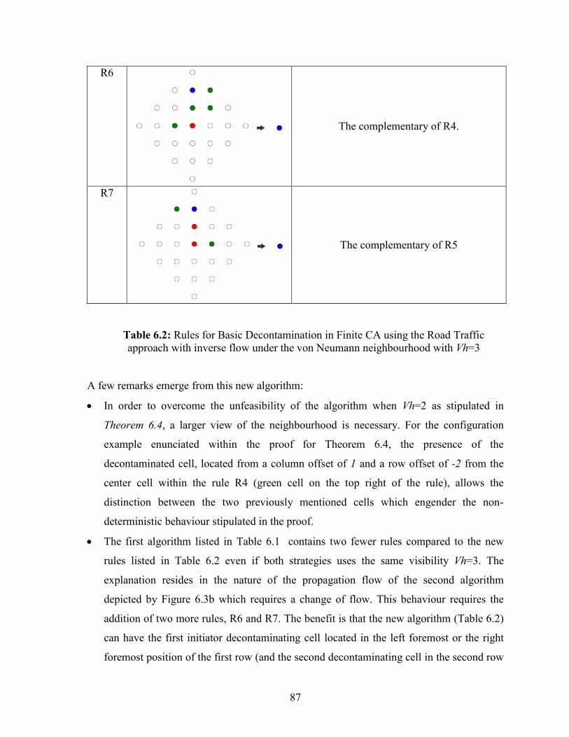
87
R6
The complementary of R4.
R7
The complementary of R5
Table 6.2: Rules for Basic Decontamination in Finite CA using the Road Traffic
approach with inverse flow under the von Neumann neighbourhood with Vh=3
A few remarks emerge from this new algorithm:
In order to overcome the unfeasibility of the algorithm when Vh=2 as stipulated in
Theorem 6.4, a larger view of the neighbourhood is necessary. For the configuration
example enunciated within the proof for Theorem 6.4, the presence of the
decontaminated cell, located from a column offset of 1 and a row offset of -2 from the
center cell within the rule R4 (green cell on the top right of the rule), allows the
distinction between the two previously mentioned cells which engender the non-
deterministic behaviour stipulated in the proof.
The first algorithm listed in Table 6.1 contains two fewer rules compared to the new
rules listed in Table 6.2 even if both strategies uses the same visibility Vh=3. The
explanation resides in the nature of the propagation flow of the second algorithm
depicted by Figure 6.3b which requires a change of flow. This behaviour requires the
addition of two more rules, R6 and R7. The benefit is that the new algorithm (Table 6.2)
can have the first initiator decontaminating cell located in the left foremost or the right
foremost position of the first row (and the second decontaminating cell in the second row
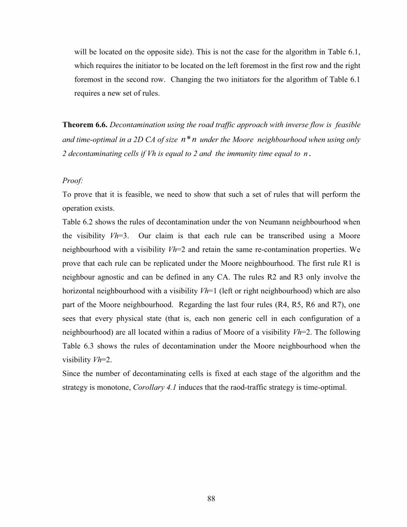
88
will be located on the opposite side). This is not the case for the algorithm in Table 6.1,
which requires the initiator to be located on the left foremost in the first row and the right
foremost in the second row. Changing the two initiators for the algorithm of Table 6.1
requires a new set of rules.
Theorem 6.6. Decontamination using the road traffic approach with inverse flow is feasible
and time-optimal in a 2D CA of size nn* under the Moore neighbourhood when using only
2 decontaminating cells if Vh is equal to 2 and the immunity time equal to n .
Proof:
To prove that it is feasible, we need to show that such a set of rules that will perform the
operation exists.
Table 6.2 shows the rules of decontamination under the von Neumann neighbourhood when
the visibility Vh=3. Our claim is that each rule can be transcribed using a Moore
neighbourhood with a visibility Vh=2 and retain the same re-contamination properties. We
prove that each rule can be replicated under the Moore neighbourhood. The first rule R1 is
neighbour agnostic and can be defined in any CA. The rules R2 and R3 only involve the
horizontal neighbourhood with a visibility Vh=1 (left or right neighbourhood) which are also
part of the Moore neighbourhood. Regarding the last four rules (R4, R5, R6 and R7), one
sees that every physical state (that is, each non generic cell in each configuration of a
neighbourhood) are all located within a radius of Moore of a visibility Vh=2. The following
Table 6.3 shows the rules of decontamination under the Moore neighbourhood when the
visibility Vh=2.
Since the number of decontaminating cells is fixed at each stage of the algorithm and the
strategy is monotone, Corollary 4.1 induces that the raod-traffic strategy is time-optimal.

89
# Configuration
Next
State Notes
R1
Any decontaminating cell will be
decontaminated in the next step.
R2
Left to Right motion on the Horizontal line
R3
Right to Left motion on the Horizontal line
R4
Jump to the next decontaminating cell on the
left vertical border.
R5
Jump to the next decontaminating cell on the
right vertical border
R6
The complementary of R4.

90
R7
The complementary of R5
Table 6.3: Rules for Basic Decontamination in Finite CA using the road Traffic
approach (with inverse flow) under the Moore neighbourhood with Vh=2
6.2.4. Similar strategies on sub networks
Looking at the strategies in the previous subsection, we note that they already carry out
a subdivision of the CA in groups of two rows, and the same movements are reapplied on
each group by finding rules to jump to the next pair of rows. Since the movements are
horizontal, we investigate another subdivision in which the CA are split by vertical cuts. The
network could be seen as a family of disjoint sub networks and each could be
decontaminated using one of the above algorithms. The idea is to subdivide the network and
split it into k truncated sub-networks as in Figure 6.5. Each truncated sub-network is then
modelled by a CA. By doing so, transition rules are applied to each sub CA according to the
strategy mentioned in the previous section.
n
n/k n/k n/k
n
a
b d
c
f
e
Figure 6.5: The cut strategy of the road traffic approach
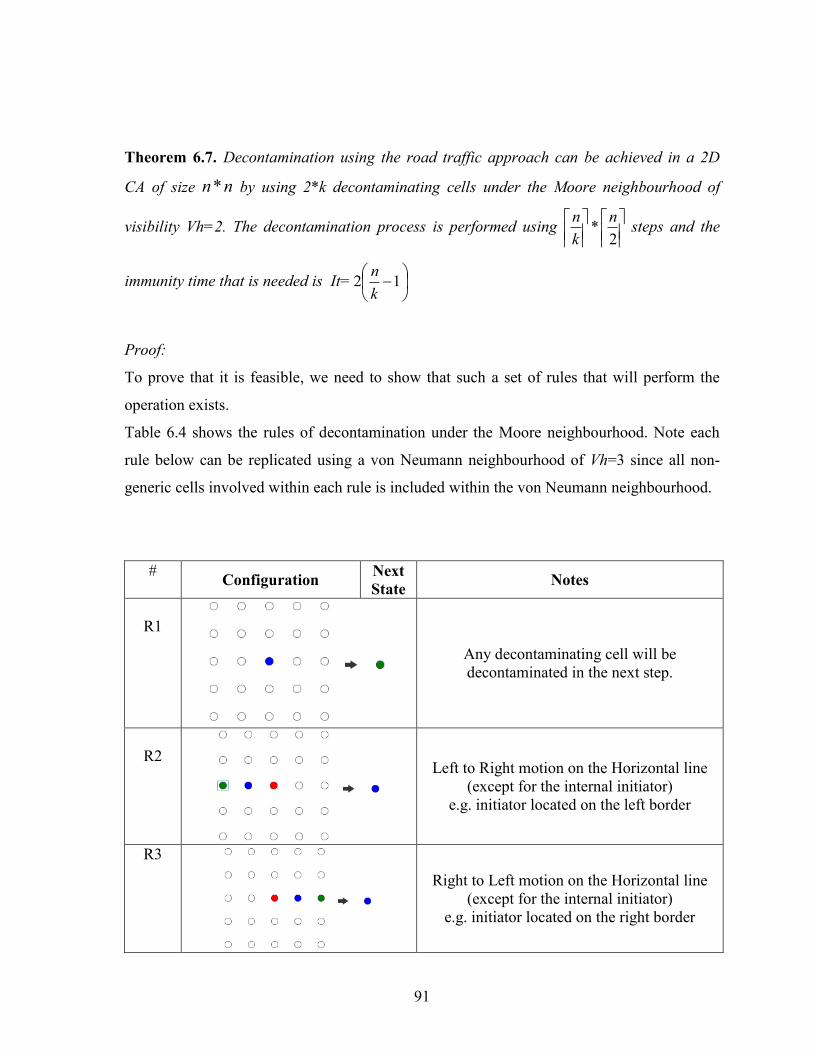
91
Theorem 6.7. Decontamination using the road traffic approach can be achieved in a 2D
CA of size nn* by using 2*k decontaminating cells under the Moore neighbourhood of
visibility Vh=2. The decontamination process is performed using
2*
n
k
n steps and the
immunity time that is needed is It=
12
k
n
Proof:
To prove that it is feasible, we need to show that such a set of rules that will perform the
operation exists.
Table 6.4 shows the rules of decontamination under the Moore neighbourhood. Note each
rule below can be replicated using a von Neumann neighbourhood of Vh=3 since all non-
generic cells involved within each rule is included within the von Neumann neighbourhood.
# Configuration
Next
State Notes
R1
Any decontaminating cell will be
decontaminated in the next step.
R2
Left to Right motion on the Horizontal line
(except for the internal initiator)
e.g. initiator located on the left border
R3
Right to Left motion on the Horizontal line
(except for the internal initiator)
e.g. initiator located on the right border

92
R4
Jump to the next decontaminating cell on the
left vertical border.
R5
Jump to the next decontaminating cell on the
right vertical border
R6
The complementary of R4.
R7
The complementary of R5
R8
Left to Right motion on the Horizontal line
of the internal initiator
e.g. internal initiator on the 1st row, 5th …
R9
Right to Left motion on the Horizontal line
of the internal initiator
e.g. internal initiator on the 2nd row, 6th …

93
R10
Right to Left motion on the Horizontal line
of the internal initiator (inverse flow)
e.g. internal initiator on the 3nd row, 7th …
R11
Left to Right motion on the Horizontal line
of the internal initiator (inverse flow)
e.g. internal initiator on the 4th row, 8th …
R12
Jump to the next decontaminating cell of an
internal cell from a left-to-right flow
e.g. 1st row to 3rd row
R13
Jump to the next decontaminating cell of an
internal cell from a right-to-left flow
e.g. 2nd row to 4th row
and its inverse left-to-right flow
4th row to 6th
R14
Jump to the next decontaminating cell of an
internal cell from a right-to-left flow
(Inverse flow of R12)
e.g. 3rd row to 5th row
Table 6.4: Rules for Decontamination in Finite CA using the road traffic approach (with
inverse flow) using 2*k decontaminating cells under Moore neighbourhood with Vh=2
The difference between the base strategy (
Figure 6.1) and the one subdivided in k sub-networks (Figure 6.5) are the insertion of
new internal cell initiators (cells b and c of Figure 6.5). Clearly, the system needs to have the
equivalent of R2, R3…R7 for these new internal cells. We also need to make sure that the
addition of these new rules is not interfering with the existing rules and vice versa.

94
1. Both rules R2 and R3 have to be more specific to target only the initiators located on the
border to avoid interfering with the rules for internal initiators. (The original definition of
R2 and R3 of Table 6.3 will set both the left and right neighbours of the internal
initiators in a decontaminating state, which we want to avoid as we want the internal
initiator to start the decontamination from one side only). Therefore, R2’s definition
will need to be replaced by .
and R3’s definition will change to .
2. We will need to add 4 new rules analogous to R2 and R3 dedicated to these internal
cells. Two new rules similar to the flow encountered on the 1st row and 2nd row are
needed (respectively R8 and R9), as are 2 other rules for the inverse flow, similarly
encountered on the 3rd and 4th row (R10 and R11).
3. We will need to add the rules that will allow the jump of an internal cell when it reaches
the extremity of the sub-network. Rule R12 will represent the jump of an internal cell
from a left-to-right flow from the 1st row to the 3rd row (and continuously from the 5th to
the 8th, etc.). Rule R4 accomplishes the same rule with its inverse flow. Additionally,
rule R13 is able to embody both rules required for the jump of an internal cell of a
normal flow (2nd row to 4th , 6th row to 8th row, etc.) and its inverse flow (4th to 6th, 8th to
10th, etc.).
4. With respect to the immunity time needed, we note that the cell which needs the most
immunity time value is the one similar to the internal cell b of Figure 6.5. Since k
n is the

95
sub-network width, 1k
n units of time are needed for its contaminated right neighbour to
reach a decontaminating state. Also, because of the Moore neighbourhood, the cell needs
another 1k
n units of time for its contaminated bottom-right neighbour to be in a
decontaminating state. All of its remaining neighbours are already decontaminated.
Therefore, the immunity time needed is
12
k
n steps.
6.3. Diagonal snake Approach
6.3.1. Base Idea
The main goal is to be able to perform the decontamination using only a single
decontaminating cell. The idea is to choose a single initiator located at the top left of our CA
and propagate in a diagonal zig-zag flow towards the opposite diagonal cell (bottom right
corner). The concept is depicted in Figure 6.6.
Figure 6.6: The diagonal snake approach within the Moore neighbourhood
Theorem 6.8. Decontamination using the diagonal snake approach can only be achieved in
a 2D CA of size nn* under the Moore neighbourhood by using a single decontaminating
cell if the immunity time is at least 2(n-1).

96
Proof:
The cell that needs the most immunity time is the decontaminated cell which needs the
longest protection time while all its direct contaminated neighbors are able to spread their
viruses. These are cells laying on the border (horizontal or vertical) of the CA (see Figure
6.6). To ensure that the cell is protected, it needs to wait for the propagation of the
decontaminating cell to navigate the entire diagonal, and to wait for the next diagonal to be
fully decontaminated for a total of two complete steps of decontaminating two diagonals. As
a comparison, an inner cell needs less as it is protected after approximately half of the
containing diagonal and the next diagonal. .
In Figure 6.7, we differentiate the cases when n is even and when n is odd since the
diagonal has the potential to be reached differently by the diagonal flow. In both cases, we
note that the cells which need the most immunity time are a or e. After e is decontaminated,
it is in danger of recontamination until d reaches the decontaminating state. In practice, this
means that e needs the entire decontamination of the diagonal {e,a} and {b,c} and the cell d
to be in a decontaminating state. Decontaminating the diagonal {e,a} needs n-1 steps and
the diagonal {b,c} needs n steps for a total of (n-1)-1+n units of time ((n-1)- because a's
immunity time begins only after a gets decontaminated). With the same logic applied to the
cell a, the cell is open to recontamination until f reaches the decontaminating state. This
means that a needs the entire decontamination of the diagonals {d,f} and {b,c}.
Decontaminating the diagonal {d,f} needs n-1 steps and {b,c} needs n steps, for a total of (n-
1)-1+n units of time.
Since the algorithm requires n steps to navigate the full diagonal and n-2 steps to navigate
the previous (or the next) diagonal, at least 2n-2=2*( n-1) units of time are needed to protect
the cell.

97
n is even n is odd
a
a
b
bc
c
d
d
e
e
f
f
Figure 6.7: Execution difference around the diagonal depending on the value of n
6.3.2. Sample Execution
At the initial stage t=0, we choose one initiator located at the top left (at coordinate
(1,1)) to start the algorithm (see Figure 6.8). At time t=1, the initiator will cause its right
neighbor, located at coordinate (1,2), to become in a decontaminating state because it sees a
flow of decontamination coming from the left. At time t=2, the cell at coordinate (2,1) goes
into a decontaminating state because it sees a flow of decontamination coming from the top-
right. At time t=3, a flow coming from the top makes the cell located at (3,1) to also be in a
decontaminating state. And at time t=4, the internal cell (1,1) goes into decontaminating
because of a bottom-right flow. In the remainder of the algorithm, cells process their state
similar to these previous stages. After examination of the flow presented Figure 6.6 and the
scrutiny of the sample execution, these various moves can be seen as the results of different
propagation flows listed in Table 6.5.

98
t=0 t=1 t=2 t=3
t=4 t=5 t=6 t=7
Figure 6.8: Propagation of the diagonal snake approach within the Moore
neighbourhood
Table 6.5 presents four distinct propagation flows coming from the left, the top, the
bottom-left and the top-right. A cell changes its state from contaminated to decontaminating
by analyzing the propagation flow and with some additional parameters. For instance, at
time t=3, one should expect that the 3rd cell of the top border (1,3) will transition into a
decontaminating state, similar to its left neighbour (1,2) at time t=2. Our claim is that these
additional parameters can be extrapolated into a Boolean function that analyzes the distant
neighbourhood of the current cell. The 3rd cell of the top border (1,3) did not transition into a
decontaminating state at time t=3 because it did not satisfy the function f1 like its left
neighbour (1,2) does at time t=2. We will show in the upcoming sections that these functions
are in fact a verification of the state of the neighbourhood of Vh=2.

99
Direction
flow
Partial
neighbourhood
configuration
Additional
input
function
Next
State Notes
Left-to-Right
f1
Horizontal flow coming from
the left with additional
restriction f1
Top-to-Bottom
f2
Vertical Flow coming from
the top with additional
restriction f2
Bottom Left
to
Top-Right
f3
Diagonal Flow coming from
the bottom left with
additional restriction f3
Top Right
to
Bottom Left
f4
Diagonal Flow coming from
the top right with additional
restriction f4
Table 6.5: Direction flow of the decontaminating transition state
We now show that consulting the direct neighbourhood is not sufficient for making a
decision with regards to the transition state definition and that additional input functions f1,
f2, f3 and f4 are required.
Theorem 6.9. Decontamination using the Diagonal snake approach cannot be achieved in a
2D CA of size nn* under the Moore neighbourhood of visibility Vh=1.
Proof:
To prove the theorem, we will show that it is not possible to find decontamination rules if
Vh=1.
To this end, we show that there are at least two cells within the CA that need to behave
differently at time t+1 (they are in different states) even if both cells have exactly the same
direct neighbourhood configuration (that is Vh=1) at time t. Indeed, having such rules makes

100
the automata non deterministic. The cells a and c in Figure 6.9 are these cells. Both cells
have the same properties as they both lay on the top border of the CA. The neighbourhood
configuration (with Vh=1) of a at time t=0 is exactly the same as the neighbourhood
configuration of c at time t=1. At time t=0, a has its left neighbour in decontaminating mode,
all remaining existing neighbours are in a contaminated state, and a does not have top
neighbours. The cell c has exactly the same configuration at time t=1 since its left neighbour,
which is a, will also be in decontaminating mode, all remaining existing neighbours are in a
contaminated state, and a does not have top neighbours. The cell a must change its state to
decontaminating in the next step (at time t=1), however, c must remain contaminated at the
next step (at time t=2). Therefore, no rules that take account of a direct neighbourhood are
feasible and thus ends our proof.
a bc
j
i
k
m no
f
e
g
r
q
a bc
f
e
g
m no
j
i
k
n is odd n is even
d
h l
p
Figure 6.9: The different type of cells within the CA during the diagonal snake strategy
Let us investigate the nature of the functions f1, f2, f3 and f4.
We take the case of the cells a and c as an example to define the nature of f1. The logic
of the definition of the other functions f2, f3 and f4 is the same. Let us consider the
configurations of the CA shown in Figure 6.10, a snapshot of Figure 6.9 at time t=0 and t=1.
Note that a is at coordinate (1,2). As observed, the Vh=1 neighbourhood configuration of
the cell a at time t=0 is exactly the same as the neighbourhood configuration of the cell c at
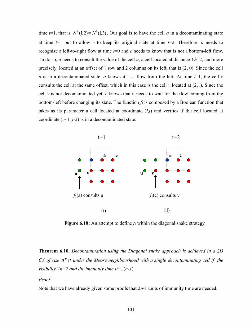
101
time t=1, that is )2,1(0N = )3,1(1N . Our goal is to have the cell a in a decontaminating state
at time t=1 but to allow c to keep its original state at time t=2. Therefore, a needs to
recognize a left-to-right flow at time t=0 and c needs to know that is not a bottom-left flow.
To do so, a needs to consult the value of the cell u, a cell located at distance Vh=2, and more
precisely, located at an offset of 1 row and 2 columns on its left, that is (2, 0). Since the cell
u is in a decontaminated state, a knows it is a flow from the left. At time t=1, the cell c
consults the cell at the same offset, which in this case is the cell v located at (2,1). Since the
cell v is not decontaminated yet, c knows that it needs to wait for the flow coming from the
bottom-left before changing its state. The function f1 is composed by a Boolean function that
takes as its parameter a cell located at coordinate (i,j) and verifies if the cell located at
coordinate (i+1, j-2) is in a decontaminated state.
a c
f1(a) consults u
ca
vvu
t=1 t=2
u
f1(c) consults v
(i) (ii)
Figure 6.10: An attempt to define f1 within the diagonal snake strategy
Theorem 6.10. Decontamination using the Diagonal snake approach is achieved in a 2D
CA of size nn* under the Moore neighbourhood with a single decontaminating cell if the
visibility Vh=2 and the immunity time It=2(n-1)
Proof:
Note that we have already given some proofs that 2n-1 units of immunity time are needed.

102
We now show that rules which fulfill the decontamination exist. To prove that these rules are
valid and that there is no collision between the rules, we analyse the flow to distinguish the
different types of cells in the CA with respect to the propagation of the flow. Figure 6.9
shows the different types of cells caused by the flow The cells a, g, i, o, q and r can
represent any cells in the CA. That is, any cell of the automata during the algorithm
execution has the same neighbourhood configuration as one and exactly one of these cells.
Therefore, each cell in the decontamination rules table, listed in Table 6.6, contains as many
rules as the number of cells previously listed.
In order to prove the validity of the rules listed in Table 6.6, a complete proof should list
each rule R2, R3, ...,R7 and validate each against any possible configuration of a, g, i, o, q
and r . An exhaustive proof should validate 6*6=36 tests. We follow with two examples of
these tests.:
Example 1: Validation of rule R2 against the configuration of r. The rule R2, defined in
gray scale mode as , is a rule that defines a left-to-right flow applied
to cells laying on the top border of the CA. We want to verify that the same rule is not
causing a left-to-right flow against r. Thus, r should keep its state unchanged even if its left
neighbour is decontaminating. At a certain time t, the decontamination reaches the left
neighbour of r and the configuration of r's neighbourhood is depicted as
ru
v
. We clearly see that the cells u and v show different states, therefore the
rule R2 is valid for the configuration of r.
Example 2: Validation of rule R2 against the configuration of q. We want to verify that
the same rule does not cause a left-to-right flow against q. Thus, q should keep its state
unchanged even if its left neighbour is decontaminating. At a certain time t, the
decontamination reaches the left neighbour of q and the configuration of q's neighbourhood
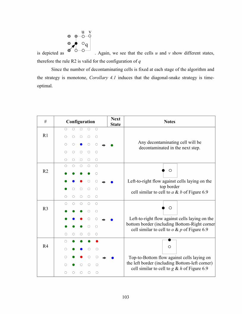
103
is depicted as
q
u v
. Again, we see that the cells u and v show different states,
therefore the rule R2 is valid for the configuration of q
Since the number of decontaminating cells is fixed at each stage of the algorithm and
the strategy is monotone, Corollary 4.1 induces that the diagonal-snake strategy is time-
optimal.
# Configuration Next
State Notes
R1
Any decontaminating cell will be
decontaminated in the next step.
R2
Left-to-right flow against cells laying on the
top border
cell similar to cell to a & b of Figure 6.9
R3
Left-to-right flow against cells laying on the
bottom border (including Bottom-Right corner)
cell similar to cell to o & p of Figure 6.9
R4
Top-to-Bottom flow against cells laying on
the left border (including Bottom-left corner)
cell similar to cell to g & h of Figure 6.9

104
R5
Top-to-Bottom flow against cells laying on
the right border
cell similar to cell to i & j of Figure 6.9
R6
Diagonal flow from the bottom left
cell similar to cell to q, k & c of Figure 6.9
R7
Diagonal flow from the top right
cell similar to cell to r, e & m of Figure 6.9
+
Table 6.6: Rules for Decontamination in Finite CA using the diagonal snake approach
move under the Moore neighbourhood when Vh=2 and for an immunity time It=2n-1
6.3.3. Division and Re-Application
The advantage of the diagonal snake method is the ability to decontaminate the
network with only one single cell decontaminating. In addition, we note that the spread is
done with a particular movement that can be easily replicated on different corners of the CA.
This is possible because of the symmetric structure of the four corners of our CA.
6.3.3.1. Case with 2 corner initiators.
The execution can be started by two corner initiators: the top-left and the bottom right
cell as shown by Figure 6.11.

105
Figure 6.11: The subdividing strategy using 2 initiators.
The idea is to replicate the execution of the top left initiator with the initiator in the
bottom-right corner. One can see that the execution of the algorithm from the bottom-right
initiator is symmetric to the execution by the top-left corner initiator. Therefore, the rule
building of this new strategy is to just use the same rule that controls the navigation of the
original flow and rotate each rule to 180 degrees. The execution of the algorithm is
completed when the two decontaminating cells meet along the diagonal of the CA.
Theorem 6.11. Decontamination using the Diagonal snake approach is achieved in a 2D
CA of size nn* under the Moore neighbourhood with 2 simultaneously decontaminating cells
if the visibility Vh=2 and the immunity time It=2n-3.
Proof:
Similar to the proof of Theorem 6.8 presented in the previous section, one can see that this
time, the cell which needs the most immunity time is the one laying on the vertical border
and located 3 rows below (or above) the corner cell containing the diagonal (the cells labeled
h and k from Figure 6.9). The protection is required during the full decontamination of the
diagonal containing the cell (n-4), the full decontamination of the next diagonal (n-1), and
the first 2 cells of the full diagonal. The total of immunity time which is required is 2n-3
units of time..
The feasibility of the algorithm is presented in Table 6.7. The first seven rules are identical
to the rules of the single initiator. The next four rules (R8, R9, R10, and R11) are added to
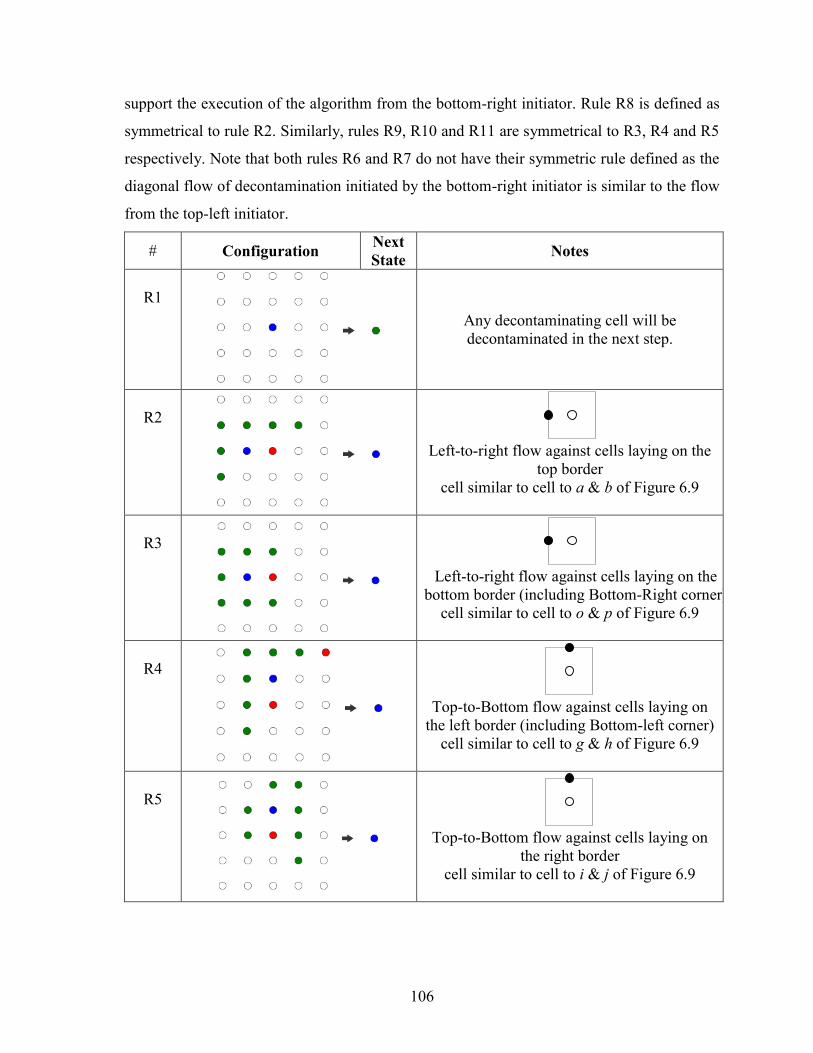
106
support the execution of the algorithm from the bottom-right initiator. Rule R8 is defined as
symmetrical to rule R2. Similarly, rules R9, R10 and R11 are symmetrical to R3, R4 and R5
respectively. Note that both rules R6 and R7 do not have their symmetric rule defined as the
diagonal flow of decontamination initiated by the bottom-right initiator is similar to the flow
from the top-left initiator.
# Configuration Next
State Notes
R1
Any decontaminating cell will be
decontaminated in the next step.
R2
Left-to-right flow against cells laying on the
top border
cell similar to cell to a & b of Figure 6.9
R3
Left-to-right flow against cells laying on the
bottom border (including Bottom-Right corner)
cell similar to cell to o & p of Figure 6.9
R4
Top-to-Bottom flow against cells laying on
the left border (including Bottom-left corner)
cell similar to cell to g & h of Figure 6.9
R5
Top-to-Bottom flow against cells laying on
the right border
cell similar to cell to i & j of Figure 6.9

107
R6
Diagonal flow from the bottom left
cell similar to cell to q, k & c of Figure 6.9
R7
Diagonal flow from the top right
cell similar to cell to r, e & m of Figure 6.9
R8
The symmetric rule of R2
R9
The symmetric rule of R3
R10
The symmetric rule of R4
R11
The symmetric rule of R5
Table 6.7: Rules for Decontamination in Finite CA using the diagonal snake approach
move with 2 corner initiators under the Moore neighbourhood of Vh=2.

108
6.3.3.2. Case with 4 corner initiators.
Figure 6.12 shows the way to cut the CA in order to produce sub-structure that it can
be processed by 4 initiators. The goal is to reuse the same strategy on these substructures. In
Figure 6.12(i), we easily retrieve the identical nomenclature of the parent because the size of
the automata is even. What is needed is only a vertical and horizontal cut which separates
our CA into 4 equal parts. To start the algorithm, the first step is to consider the four cell
corners as initiators and execute the same strategy as in the base case (Figure 6.12a). The
algorithm stops when the 4 central cells of our CA are decontaminated.
In Figure 6.12(ii), due to the size of the automata being odd, the CA could not be split
into four equal parts. Obviously, there is always a possibility of splitting it into unequal
blocks as suggested by Figure 6.12d. In this situation, the grid shall be divided into four
parts of equal size plus one isolated single cell. The subdivision always holds when n is odd.
Since n=2k+1, we can easily deduct that 1))1((4)12( 22 kkkn . Therefore, the size
of each block is )1( kk .
Proposition 6.1. Decontamination using the Diagonal snake approach can be achieved in a
CA under the Moore neighbourhood with 4 decontaminating cells if the visibility Vh=2 and
the immunity time 12
*2
nIt
By looking at the behaviour of the decontamination flows between a CA of even size
(see Figure 6.12(i)) and of an odd size (see Figure 6.12(ii)), we can see that the
decontamination flow is similar in the early stage of the decontamination until the
subdivided blocks meet on the border. For an even sized CA, the decontamination flow is
resumed with a vertical or horizontal flow (Figure 6.12b). Conversely, the flow is resumed
in a diagonal way for an odd sized CA (Figure 6.12d). The difference of execution
automatically implies that the set of transition rules is different. The complexity of building
the contamination rules for both cases is perceptible because one can see new configurations
of neighbourhood arising. Therefore for both strategies, we have shown experimentally that
decontamination is feasible and we have validated its feasibility by generating the rules
using the research tool we have designed and that we present in the next chapter.

109
(a)
(b)
(ii)(i)
(c)
(d)
n is oddn is even
Figure 6.12: The subdividing strategy using the snake approach with 4 initiators
6.4. The subdividing strategy of the Diagonal Move Approach
In order to put the focus on the concept of subdivision, we consider the simplest
diagonal approach which is the case of Vh=1 and Cd=1 as presented in Chapter 5. Indeed,
the strategy of implementing the subdivision will be similar even for arbitrary values of Vh
and Cd. We also recall that the topology that we consider is the n*n grid under the von
Neumann neighbourhood. Besides, the value of the time of immunity is null since the base
Diagonal Move performs without any Immunity.

110
Aside from the motivations dedicated to the diagonal move already mentioned in
Chapter 5, another attractive property of the method is that its simple move pattern allows
the launch of the diagonal movement from different areas of our CA.
6.4.1. Case with 2 corner initiators
Given that the motion pattern is from diagonal to diagonal, the most natural cut is to
subdivide the CA into two triangles and begin decontamination from the two opposite
corners of the triangles as suggested in Figure 6.13 (that is, from two corners of the CA
diagonally opposite). For this, the algorithm just needs two initiators and starts
decontamination diagonally as presented in Chapter 5. Taking the cell at the top-left corner
as a decontaminating initiator will cause a flow to the right and downwards, while a
decontaminating cell at the bottom-right corner will cause a flow to the left and upward.
Eventually the two diagonals meet to stop decontamination. This process bring us to the next
theorem.
Theorem 6.12. Decontamination using the Diagonal approach is achieved in a 2D CA of
size nn* under the von Neumann neighbourhood with 2 initiators decontaminating cells
during n units of time. Immunity time is not required

111
(a)
(b)
Figure 6.13: The divide and conquer diagonal strategy with 2 initiators
Proof:
Table 5.1 of Chapter 5 displays the rules for decontamination in Finite CA using basic
diagonal move with the von Neumann neighbourhood when Vh=1 and Cd=1 with a single
decontaminating cell initiator located on the top left of the CA. The rules were built
according the type of cell for being either a cell laying on the border (R2 and R3) or an
internal cell (R4). It is easy to see that the flow of decontamination started by a second
initiator on the bottom right is diametrically symmetric to the flow of decontamination by
the first initiator from the top left cell. Therefore, the new flow can be realized by adding
new rules that are diametrically symmetric to R2, R3 and R4 which are R3, R4 and R5
respectively as seen in Table 6.8.
.

112
# Configuration
Next
State Notes
R1
Any decontaminating cell will be
decontaminated in the next step.
R2
Cell located on the top horizontal border of
the CA
R3
Cell located on the left vertical border of the
CA
R4
Internal Cell
R5
Diametrically symmetric to R2
Cell located on the bottom horizontal border
of the CA
R6
Diametrically symmetric to R3
Cell located on the left vertical border of the
CA
R7
Diametrically symmetric to R4
Internal Cell
Table 6.8: Rules for Basic Decontamination in Finite CA using basic diagonal move and
two corner initiators under the von Neumann neighbourhood when Vh=1 and Cd=1
6.4.2. Case with 4 corner initiators
We saw that it was possible to reuse the diagonal approach with 2 decontaminating
cells with the CA in two triangles. What is proposed in Figure 6.14 is the use of 4
decontaminating cells. We start the decontamination from the four corners of our CA. The
decontaminating cell located at the top-left corner will propagate a flow to the right and

113
downward. Similarly, the decontaminating cell at the bottom-right corner will cause a flow
to the left and upward, the cell to the top-right corner will propagate a flow to the left and
downward, and finally the decontaminating cell at the bottom-left corner will propagate a
flow to the right and upward. Implicitly, this strategy cuts the CA into four equal parts if n is
even (Figure 6.14f) and in unequal parts if n is odd (Figure 6.14c). In the first case,
decontamination ends when the 4 centre cells of the CA get decontaminated. In the second
case, the decontamination of the cell at the centre of our CA marks the end of the algorithm
execution. This strategy is supported by the theorem below
Theorem 6.13. Decontamination using the Diagonal approach can be achieved in a 2D CA
of size nn* under the von Neumann neighbourhood with 4 decontaminating cells. The
algorithm execution requires 12
*2
n units of time The maximum number of
decontaminating cells encountered during the execution is
2*4
n.
.
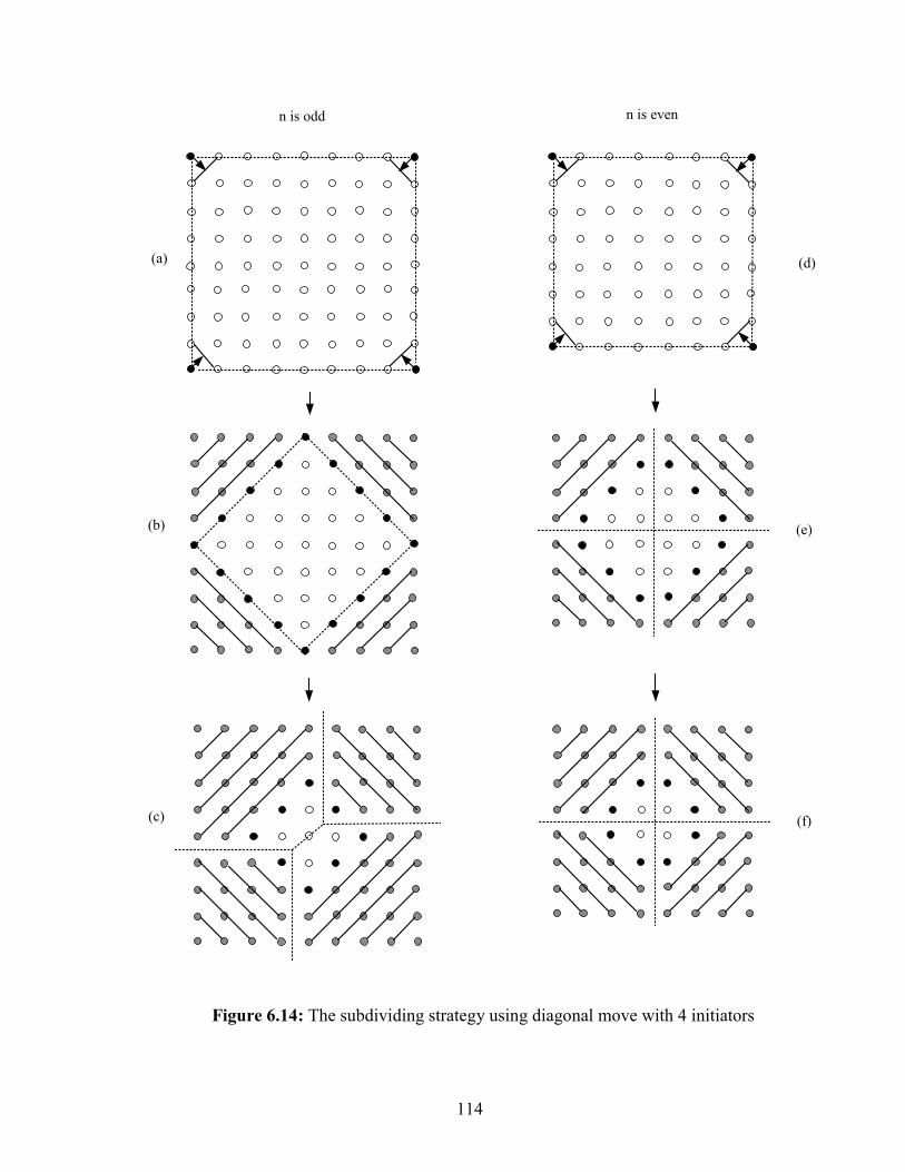
114
(b)
(a)
(c)
n is odd n is even
(e)
(d)
(f)
Figure 6.14: The subdividing strategy using diagonal move with 4 initiators

115
Proof:
By using the same techniques presented in the proof of Theorem 6.9, the rules for four
corner initiators can be built in two different ways. The first option is to start with the three
rules R2, R3 and R4 and symmetrically transpose these rules diametrically (R5, R6 and R7),
vertically (R8, R9 and R10) and horizontally (R11, R12 and R13). Obviously, the three latter
rules are vertically symmetric to R5, R6 and R7. These results are listed in Table 6.9. To
prove that 12
*2
n units of time is needed to achieve the decontamination, we proceed by
analogy with the decontamination of a CA of Cd=1 and Vh=1 with a single initiator which
requires 12 n units of time. The decontamination duration of a nn * CA with four
initiators is similar to the execution of the
2*
2
nn CA with a single initiator as the CA is
split into four parts. This can be easily noticed when looking at Figure 6.14c when n is odd
or Figure 6.14f when n is even. Therefore, by replacing n with
2
n in 12 n , we can
deduce that the decontamination time is 12
*2
n.

116
# Configuration
Next
State Notes
R1
Any decontaminating cell will be
decontaminated in the next step.
R2
Cell located on the top horizontal border of
the CA
R3
Cell located on the left vertical border of the
CA
R4
Internal Cell
R5
Diametrically symmetric to R2
Cell located on the bottom horizontal border
of the CA
R6
Diametrically symmetric to R3
Cell located on the left vertical border of the
CA
R7
Diametrically symmetric to R4
Internal Cell
R8
Vertically symmetric to R2
Cell located on the bottom horizontal border
of the CA
R9
Vertically symmetric to R3
Cell located on the left vertical border of the
CA

117
R10
Vertically symmetric to R4
Internal Cell
R11
Horizontally symmetric to R2
Vertically symmetric to R5
Cell located on the bottom horizontal border
of the CA
R12
Horizontally symmetric to R3
Vertically symmetric to R6
Cell located on the left vertical border of the
CA
R13
Horizontally symmetric to R4
Vertically symmetric to R7
Internal Cell
Table 6.9: Rules for Basic Decontamination in Finite CA using basic diagonal move and
four corner initiators with the von Neumann neighbourhood when Vh=1 and Cd=1
6.4.3. Case with 3 corner initiators
It is important to note that the algorithm covers the scenario of three corner initiators,
regardless of which three cells among the four corner initiators are selected. Since the
transition rules covers all flows (top-left to bottom-right, top-right to bottom-left, bottom-
right to top-left, bottom-left to top-right), the algorithm supports any execution started from
any number of corner initiators (that is one, two, three or four initiators) and any
combination of two or three corner initiators from any corner location. For instance, Figure
6.15 shows an execution of the divide and conquer diagonal move algorithm defined in
Table 6.9 with a single corner initiator on the top-right (Figure 6.15a), two initiators located
on the top-left and the bottom-left (Figure 6.15b), and three initiators sited on the top-right,
bottom-right and bottom-left (Figure 6.15c).

118
Figure 6.15: A sample of execution of the subdividing strategy using diagonal move
algorithm using a dynamic number of initiators.
Theorem 6.14. Decontamination using the Diagonal approach can be achieved in a 2D CA
of size nn* under the von Neumann neighbourhood with 3 decontaminating cells. The
algorithm execution requires n units of time The maximum number of decontaminating cells
encountered during the execution is
2*3
n.
Proof:
Any algorithm with four initiators will perform when three initiators are chosen, so Table 6.9
can then be used as the set of rules. Regarding the duration of the decontamination, n units of
time are needed. One can see that the last cell to be decontaminated is the corner that was
not selected as an initiator. The last corner cell can only be decontaminated after it is reached
by the decontamination flow coming from its adjacent and horizontal (or vertical) corner,
similar to the execution by two initiators. Therefore, n steps are needed. Following the same
logic shown in the proof for Theorem 6.13, the maximum number of
2*3
ndecontaminating cells is reached at time 1
2
nt .
6.4.4. Rules minimization
In the previous section, the construction of the rules has been based on basic rules that
act on a single initiator (top-left) and the transposition of these basic rules to create new rules
based on the symmetry of execution. The basic rules are composed of three transition rules

119
based on the location of the cell within the CA, laying on a border (vertical or horizontal), or
defined as an internal cell. Then, each rule is transposed. With this methodology, we manage
to create the algorithm listed in Table 6.9. The three basic rules are transposed vertically,
horizontally, and diagonally which gives a total of 12 rules. A good question is to ask if the
same strategy can be performed with fewer rules. With respect to the diagonal move
strategy, there are two different approaches that can be taken to minimize the number of
rules.
6.4.4.1. Approach by “flow analysis”.
# Configuration
Next
State Notes
R1
Any decontaminating cell will be
decontaminated in the next step.
R2
Rule triggering an horizontal flow
R3
Rule triggering a vertical flow
Table 6.10: Alternative rules for Basic Decontamination in Finite CA under the von
Neumann neighbourhood using basic diagonal move and initiated by the top left initiator
when Vh=1 and Cd=1
The first approach is to revisit the set of basic rules and try to minimize them. To do
so, instead of producing rules that are based on the type of cell, one can concentrate on the
type of flow that is propagated within the CA. A diagonal flow can be seen as both an
horizontal and vertical propagation of the decontamination. Thus, the algorithm depicted by
Figure 5.2 and defined in Table 5.1 with three rules can be improved by the simple rules
defined in Table 6.10 above.

120
We can use the same transposition strategy in Table 6.10 to create the set of rules
which can handle the execution with multiple initiators. A natural inclination is to think that
one will need 6 additional rules to perform the execution in a case with 4 initiators. The
reason for this assumption is both rules R2 and R3 have to be symmetrically transposed for
each remaining corner (vertically for the top-right corner, diagonally for the bottom-right
corner, and horizontally for the bottom-left corner). However, Table 6.11 shows that only 2
additional rules are needed to perform the entire decontamination. The vertical transposition
of R2 and R3 to satisfy the flow initiated by the top right corner is embedded in R4 and R3
respectively. Similarly, the horizontal transposition of R2 and R3 to satisfy the flow initiated
by the bottom left corner is contained in R2 and R5 respectively. Finally, the diagonal
transposition of R2 and R3 is R4 and R5 respectively. Thus, the decontamination using a
diagonal flow started by up to 4 corner initiators can be fulfilled with exactly 4
decontamination rules.
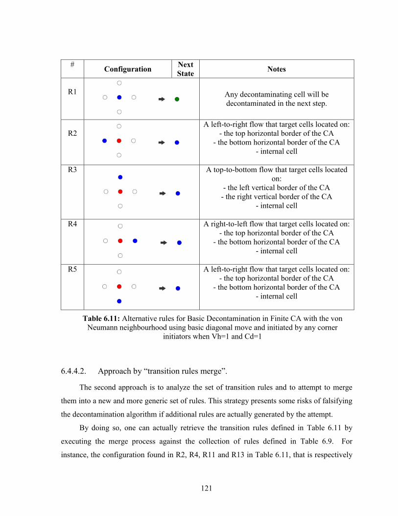
121
# Configuration
Next
State Notes
R1
Any decontaminating cell will be
decontaminated in the next step.
R2
A left-to-right flow that target cells located on:
- the top horizontal border of the CA
- the bottom horizontal border of the CA
- internal cell
R3
A top-to-bottom flow that target cells located
on:
- the left vertical border of the CA
- the right vertical border of the CA
- internal cell
R4
A right-to-left flow that target cells located on:
- the top horizontal border of the CA
- the bottom horizontal border of the CA
- internal cell
R5
A left-to-right flow that target cells located on:
- the top horizontal border of the CA
- the bottom horizontal border of the CA
- internal cell
Table 6.11: Alternative rules for Basic Decontamination in Finite CA with the von
Neumann neighbourhood using basic diagonal move and initiated by any corner
initiators when Vh=1 and Cd=1
6.4.4.2. Approach by “transition rules merge”.
The second approach is to analyze the set of transition rules and to attempt to merge
them into a new and more generic set of rules. This strategy presents some risks of falsifying
the decontamination algorithm if additional rules are actually generated by the attempt.
By doing so, one can actually retrieve the transition rules defined in Table 6.11 by
executing the merge process against the collection of rules defined in Table 6.9. For
instance, the configuration found in R2, R4, R11 and R13 in Table 6.11, that is respectively

122
depicted as , , , can be merged into . Since
the result state of these rules is identical (decontaminating), the rules R2, R4, R11 and R13
of Table 6.9 can be merged into a more generic rule, which is the rule R2 in Table 6.11.
Since all possible combinations of states are being represented, it is important to note that no
additional rules is being implicitly added by the creation of R2.
By applying the same merge strategy, the rules R3, R4, R9 and R10 of Table 6.9 are
merged into rule R3 of Table 6.11. Also, the rules R5, R7, R8 and R10 of Table 6.9 are
merged into rule R4 of Table 6.11. Finally, the rules R6, R7, R12 and R13 of Table 6.9 are
merged into rule R4 of Table 6.11. By an exhaustive count, all rules of Table 6.9 are
represented by at least one rule defined in the Table 6.11.
6.5. Summary
In this chapter, we started by introducing two new algorithms named Road traffic and
Diagonal Snake. We used these algorithms as a foundation to implement new strategies by
applying the base idea within different cuts of the CA. This allowed us to use different
number of initiators as needed. We completed the chapter by studying the technique that
accomplishes the same recursive idea using the base diagonal flow algorithm introduced in
Chapter 5. A summary of results established in this chapter is listed in the following table.

123
Strategy N*
Type Vh Cd It
Number
of
Initiator
s
Max
D*ing
cells
Time Ref.
Road Traffic
CF VN
3
1 12 n 2 2 n
n*
2
Th. 6.3
Road Traffic
IF VN
3
1 n 2 2 n
n*
2
Th. 6.5
Road Traffic
IF Moore 2 1 n 2 2 n
n*
2
Th. 6.6
Road Traffic
IF Moore 2 1
12
k
n k2 k2
2*
n
k
n Th. 6.7
Diagonal
snake Moore
2
1 12 n 1 1 2n Th. 6.8
Diagonal
snake Moore
2
1 32 n 2 2 2
2n
Diagonal
snake Moore
2
1 1
2*2
n
4 4 4
2n Prop 6.1
Diagonal
Move VN 1 1 0 2 n n Th. 6.12
Diagonal
Move VN 1 1 0 3
2*3
n n Th. 6.14
Diagonal
Move VN 1 1 0 4
2*4
n 1
2*2
n Th. 6.13
Table 6.12: Summary of decontamination results of a n*n CA using the Road Traffic,
Diagonal Snake and Diagonal Move strategy.

124
Chapter 7
7. CAEDISI, a CA editor and simulator
for Network Decontamination
In this chapter, we present a software [RZ13] that we have implemented with the aim to
support the theoretical study of Network Decontamination using CA. The initial goal was to
have simple software which could rapidly display the execution of a decontamination
algorithm instead of scribbles on paper which is tedious and arguably unreliable. The final
product is a research tool that not only acts as a simulator but also as an editor, a validation
tool, and even as a rule generator for CA.
7.1. Motivation
7.1.1. Needs and existing software limitations
In previous chapters, we presented ideas whose ultimate goal was to provide
decontamination algorithms. Obviously, the first question asked after the creation of an
algorithm is about its feasibility even before judging its performance. Initially, the
algorithm's execution was written and drawn on a sheet of paper. In the simplest cases, it
was found that the verification of these algorithms is a tedious task, even just with respect to
its correctness. It was then clear that simulation software was essential to our research.
The first step was to find existing software that could fulfill our needs. Not
surprisingly, we found the existence of a considerable amount of software that simulates the
execution of CA. Most of the software processing CA often deals with its natural form, that
is, with two states and with a direct distance in the neighborhood. The limitation of having
only two states (typically the "on" and "off" states) as stipulated in the original definition of
a CA is important because in the field of Network Decontamination, the set of transition

125
states necessarily contains at least three states: contaminated, decontaminated, and
decontaminating. In our research, we added a new state called absent (see Chapter 3) in
order to study the decontamination algorithms of sub-truncated mesh. Some software
supports the addition of new transition states or has its own way of expressing access to a
wider area of the neighbourhood within the transition rule definition, but the use of the
system turns out to be difficult and challenging. In our study, the requirement of writing
transition rules using an extended visibility of the neighbourhood is essential.
There are other limitations which are technical rather than conceptual. Most existing
software that interacts with CA are mainly simulation programs characterized by static
features with respect to the characteristics of the CA model, including its grid (the size,
visual appearance, etc.) and the definition of the neighbourhood. In some cases, the rules
governing changes of the states of each cell are predefined and static in the code. This forces
the researcher to dive into the source code of the program to update an existing algorithm or
to implement a new algorithm. Thus, a researcher must necessarily have a fairly advanced
knowledge of computer programming in order to have a visual overview of the heuristic that
he wants to implement.
The major limitation of existing software is the inability to handle some of the
additional parameters required by our study on Network Decontamination. This restriction is
manifested by the system inflexibility of integrating of such properties. One example is that
in our study, we needed a system that could support the integration of the Time Immunity
parameter within the logic of updating the state of a CA's cell. Unfortunately, we could not
find any system that offered the functionality or software that used similar functionality to
accomplish this integration.
The need for software that can implement at least these three parameters (extended
neighbourhood visibility, Contamination Distance, and Time Immunity) are among the main
motivations to create our own CA software.
7.1.2. Overall characteristics
Usable. The software is using modern technologies which makes the software easy to
use and does not require any special training. A user does not need any knowledge of
programming in order verify its algorithm. For instance, visual controls have been used to

126
input transition rules instead of the traditional notation (string character) which gives a better
visual representation of the rules.
Interactive. The software makes an effort to display informational, warning, or error
messages. For instance, the system warns the user with pop-up messages when rules are not
valid and allows the user to choose between corrections to the rules assuming a non-
deterministic behaviour. Another example is that each cell state can be explored during
simulation for more information around its attributes, such as the rule responsible for the
current state result or its immunity time value at each stage. The software also provides the
user with the ability to run the entire simulation in a continuous fashion (start to end with a
stop condition) or in a step-by-step mode.
Generic. The system can process any CA in a non-static approach. All properties of
CA are dynamic including the specification of the neighbourhood, the width, the height, the
value of the Visibility Hop, and the Contamination Distance. The software is capable of
creating and editing CA of any size. The user can choose to define any transition state, not
only the usual three states for decontamination. The system supports any type of
neighbourhood of any radius. The system will include the von Neumann and Moore
neighbourhoods by default but the user can also define and save a new type of
neighbourhood. When this case arises, the system can recursively compute the new extended
neighbourhood when the Visibility Hop increases. A user can choose to test the same
algorithm with a different topology such as tori (circular), with a different width and height,
different visibility, different immunity, and different Contamination Distance. Furthermore,
there is no limit (except machine memory) to the number of transition rules that can be
edited (created, updated, or removed) at the user's request.
Configurable. All possible fields that can be configured in the system are
configurable. For instance, the user can choose to consider the cell outside the CA as either
"absent" or "decontaminated," or even another new defined state. The user can choose to end
the simulation when a specific state of the CA is reached (e.g., all decontaminated or all
contaminated) or after a number of steps, or can choose to run the simulation indefinitely.
The visual aspects of the system are also configurable. For instance, the user can choose the
color assigned to each state.

127
Complete. The system has been tailored to include some Network Decontamination
parameters but can still be used to simulate the native form of a CA. During the simulation
mode, contamination rules are generated on demand and not by default in order for the set of
collection rules to be network contamination agnostic. For example, a user can simulate the
execution of the "game of life" CA. The program will offer a rigorous method of validation
of the rules, meaning the software will make sure that the configured CA is a deterministic
automata. The software also provides some statistical data on the execution of the algorithm.
Collaborative. Additional effort has been made to make the system a collaborative tool
for researchers. For instance, the system allows a user to register before its use. All collected
data are stored in a database that can be questioned as required. A user can create new
neighbourhood type and the latter can be reused by other users. Another example is that a
user can have view access to algorithms created by others.
Portable. The software can be deployed as a standalone application on a desktop and
can also be deployed on the web and accessed through a browser.
Advanced. The software is built using the latest technologies which makes it extensible
for the future. It has technologies such as rich internet applications (RIA), object relational
mapping (ORM with Entity Framework), web services (WCF RIA web services) and
support for the installation of the database in the cloud.
7.2. Caedisi versus current CA Software
In this subsection, our purpose is to point out the particularity and strength of
CAEDISI against current CA software. The effort has been made to bring comparisons
against the most used CA simulator currently available in order to show its contributions.
Mainly, we put the focus on its structure (including the data structure) and the approach
difference with respect to the simulation functionality. We also highlight new features that is
only found in Caedisi.
7.2.1. CA Structure
The Table 7.1 is a summary of difference between the overall data structure of Caedisi
and its pairs. Most existing software saves the CA into an Array because it is the natural
representation of a grid. However, with respect to its data structure, Caedisi saves the CA
using a new structure named “Entity” in which relational data are already structured in a

128
graph similarity. In our case, it provides more flexibility especially when the neighbourhood
is un-regular. Indeed, instead of computing the neighbours using an offset system,
neighbours are already traced through implicit edge connections.
CA Properties
Wolfram’s
MATHEMA
TICA
JCASIM MCELL GOLLY CAEDISI
CA data structure Array Array Array Array
graph of
relational
data
Supported CA
Dimensions 1D, 2D, 3D
1D, 2D,
3D 1D, 2D 1D, 2D
2D,
Open for 3D
Dynamic
neighbourhood
structure
✓
Transition rule data
structure Tree Tree Tree
Table &
Tree
Relational
data (graph)
Support multiple states limited limited limited
< 256
limited
< 256 ✓
Support larger radius ✓
Support circular CA 1D only ✓
Support Unbounded ✓ ✓ ✓ ✓
✓
(with custom
state for
unbounded
cells)
Table 7.1: CAEDISI vs current CA Software (Overall structure)
One of key difference between Caedisi and its converse is the ability to define any new
neighbouring structure of radius r=1 and the software will be able to recursively compute
any new neighbouring structure of larger radius. Even if the new neighbouring structure is

129
asymmetric (for instance, Moore and von Neumann neighbourhood are symmetric), the
software is able to generate the correct transition rule structure (see for instance Figure 7.3
with von Neumann Vh=2 and Figure 7.10 for Moore Vh=1)
Obviously, Caedisi support larger radius (Vh and Cd) and 2D circular CA which are
not found in current software. Another new functionality is to be able to specify an arbitrary
state for “imaginary” cells outside the boundary of the 2D grid. Instead of controlling the
grid offsets like the other software (for instance, a negative row index of a top neighbour
means the current cell is on the 1st row) , Caedisi is flexible and assume that cells outside the
boundary can be of any state: “Absent”, ‘Clean” , “decontaminated” or even a newly
defined state. This idea is more realistic for Network decontamination because these
unbound cells might be mapped to machines that are outside the infected network, or even
just machines with an unknown state.
Another particular strength of Caedisi is the ability to dynamically generate the
transition rule GUI configuration based on an arbitrary neighbourhood type and the value of
Vh. (for instance see Figure 7.3 with von Neumann Vh=2 and Figure 7.10 with Moore
Vh=1). The generation of the transition rule is derived from the recursive version of the
well-known graph BFS algorithm (breadth-first-search) with the pseudo-code below:
__________________________________________________________________________
Procedure GenerateGenericTransitionRule(
NeighbourhoodType NT,
int Vh)
begin
Let TR be a TransitionRule: output
int minOffset Vh * (-1);
int maxOffset Vh * (1);
int xIndexCenterCell maxOffset;
int yIndexCenterCell maxOffset;
int zIndexCenterCell 0;
int currentRadiusIndex 0;
call Procedure GenerateNeighboursData (TR, xIndexCenterCell,
yIndexCenterCell, zIndexCenterCell, NT, currentRadiusIndex, Vh)
End
__________________________________________________________________________
As for most recursive function, the previous function is the initial set up which role is
to only call the following procedure being called recursively within its body. Below, we
display the partial content of the procedure but the user can easily deduce the content of the
absent lines of code.

130
__________________________________________________________________________
Procedure GenerateNeighboursData(
TransitionRule TR,
int xIndexCenterCell,
int yIndexCenterCell,
int zIndexCenterCell,
NeighbourhoodType NT,
int currentRadiusIndex,
int Vh)
begin
Let xIndex, yIndex, zIndex be int variables
Let Q be a queue (we use it to store neighbours already being
generated)
CurrentRadiusIndexcurrentRadiusIndex+1
if (CurrentRadiusIndex > Vh)
Return
if NT.IsTopLeftOn is true
xIndex xIndexCenterCell-1
yIndex yIndexCenterCell-1
zIndex 0
Generate the cell in the UI at coordinate (xIndex, yIndex, zIndex)
Q.enqueue (Tuple(xIndex, yIndex, zIndex))
if NT.IsTopOn is true
xIndex xIndexCenterCell-1
yIndex yIndexCenterCell
zIndex 0
Generate the cell in the UI at coordinate (xIndex, yIndex, zIndex)
Q.enqueue (Tuple(xIndex, yIndex, zIndex))
if NT.IsTopRightOn is true
...
if NT.IsRightOn is true
...
if NT.IsBottomRightOn is true
...
if NT.IsBottomOn is true
...
if NT.IsBottomLeftOn is true
...
if NT.IsLeftOn is true
xIndex xIndexCenterCell
yIndex yIndexCenterCell-1
zIndex 0
Generate the cell in the UI at coordinate (xIndex, yIndex, zIndex)
Q.enqueue (Tuple(xIndex, yIndex, zIndex))
While Q is not empty
Tuple (x,y,z)dequeuer (Q)
GenerateNeighboursData(TR, x,y,z, NT, currentRadiusIndex, Vh)
end
__________________________________________________________________________

131
The operation is accomplished with O(n) operations with n being the cardinality of the
neighbours surrounding the current cell. Details about the implementation of the algorithm
can be found in [R13] under the procedure name GenerateGenericTransitionRule.
7.2.2. Simulation properties
Simulation Properties
Wolfram’s
MATHEMA
TICA
JCASIM MCELL GOLLY CAEDISI
Colouring states ✓ ✓ ✓ ✓ ✓
(with tags)
rules insertion Scripts
Code,
CDL
UI Input
Code
(external
dlls)
Scripts UI input
Support CA Editing
during execution ✓
Conditional Execution
Stop ✓
Support continuous
execution ✓ ✓ ✓ ✓
✓
(with stop
condition)
Support sequential
execution (play, pause,
steps, etc)
✓ ✓ ✓
✓
(with jump to
end according
to stop
condition)
Simulation Execution
recorder ✓
Simulation Metadata ✓
(stats

132
available at
each step)
Support Stochastic
CA
Unique
probability
(Domany-
Kinzel only)
✓
(Different
probability for
each rule)
Support non-
deterministic CA
✓
(states based-
rules or user
input)
Table 7.2: CAEDISI vs current CA Software (Simulation properties)
Some of the drawback of existing software (except JCASim) are the incapacity of
inserting new rules without, either implementing program code intervention or writing
scripts. These latter require a prior knowledge of the programming language, the script
language and the insertion protocol. Instead, Caedisi can add new rules by simple interaction
with the software. (Process is explained in further sections).
CA Editor.
Another primordial feature that is only available in Caedisi is the ability to edit the CA
during execution. The user can pause the execution and arbitrarily change any state of any
cell of the CA. The user can also consult any metadata property currently available, for
instance the circumstances that lead into a specific state of an arbitrary cell. For instance,
this functionality is needed for Network decontamination if there is a desire to investigate
random faults during decontamination in which some already decontaminated hosts gets re-
contaminated again.
Recording Execution.
Another new feature is the ability to record any execution and save it to the database for
further consultations. It is important to note that current software only save the rules so that
they can re execute the simulation in a later date. However since Caedisi allows the user to

133
edit the CA during the execution and possibly alter any states, it was necessary to have a
“read-only” version of the execution without executing again the transition rules.
Stochastic CA.
The software also supports stochastic models that can be factored by probability on the
Transition rules. The idea is to implement probabilistic model that is firstly relevant for
Network Decontamination. One of the future variation of our study is to study realistic
probabilistic model. For example, a very realistic situation is that every machine do not
always gets decontaminated but instead the cleaning process is associated with a probability
of success. For network decontamination, several situation arises, for instance:
1. Decontamination is (not) successful because of the quality of antiviral program. In
this case, any transition rule from a decontaminating state into a decontaminated
state is factored by a probability p. Therefore, the same value of p is applied to
every candidate cell transiting into the previously mentioned transition state.
2. Decontamination is (not) successful in certain machines because of the machine
characteristics (for instance, different hardware, different operating systems, etc).
In this case, each cell has its own probability q that affects any transition rule
applied to it.
3. The probability of the antiviral program of being successful increase when
executed multiple times on the same machine. In this case, faults become
dependent.
4. Also, we can see that both p and q can be both applies concurrently which gives
different stochastic models.
Currently, Caedisi implements the case 1 above.
Non-determinist CA.
Furthermore, Caedisi can execute non-deterministic CA. The resulting state to be taken in
account is
- either an interactive choice given to the user or
- an optimistic or pessimistic model configured within the software. In an optimistic
model, the order of resulting state to be chosen is

134
decontaminated>decontaminating>contaminated in this order. Conversely, in a
pessimistic model, the contaminated state gets the priority to be selected first.
7.2.3. Inverter and Reversability
INVERTER &
REVERSABILITY
Wolfram’s
MATHEMA
TICA
JCASIM MCELL GOLLY CAEDISI
Transition Rules
Generator ✓
Determinism/Non-
determinism Test ✓
Heuristic for
Reversability Test ✓
Table 7.3: CAEDISI vs current CA Software (Inverter and Reversability)
The principal functionality that dissociate Caedisi from current simulation software is
the ability to act as a rule generator. The general idea is to grab some given arbitrary
execution (inputted by the user) and the software tries to reconstruct the rules that lead to
that execution. It is easy to see that the same approach can be used as a heuristic to test the
reversibility of a given CA who is known to be NP-Hard [Kar90]. Furthermore, the test of
reversibility can be executed for a larger radius (For instance, the CA might not be reversible
for r=1 but be successful for r=3) . Note that this functionality is scrutinized in upcoming
sections of this chapter.
7.2.4. Database, Libraries and Software properties
The Table 7.4 below lists the various differences between Caedisi and various software
with respect to structure used to save the CA. One can see that Caedisi uses a standard
format to save the CA and the execution path as well. We note that current software saved
its CA into proprietary format that is usually employs text based encoding. Even if the latter
format is highly portable, issues rises when we want to complement the CA with metadata
because the new data structure was not intended to be upgraded. (For instance, saving an

135
execution using RLE appears to show some complexity). Apart the fact that a SQL format
can support any relational structure, the advantage of using it gives the researcher an ability
to use advanced data mining tools (SQL is a standard format) and have a better alternative to
study its dynamical properties (e.g. in opposition of custom format in which a plugging
needs to be coded in order to translate the format).
Artifacts
Wolfram’s
MATHEMA
TICA
JCASIM MCELL GOLLY CAEDISI
DATABASE & LIBRARIES
File Savings Proprietary
CDF
Custom
Custom
RLE
Image
format
(bmp,
tiff…)
Standard
Inside a
SQL
database
File Openings From Disk
CDF
From Disk
CDL
From Disk
RLE, Mcel,
Life, dbLife
From Disk
RLE, Mcel,
Life
From
database
CA Libraries format Proprietary
format CDL File logs File logs SQL tables
Execution records ✓
(SQL tables)
SOFTWARE PROPERTIES
Programming
Language
C/C++, Java,
Fortran, C# Java
Java Applet
Desktop
UI: XAML
Code: C#
Database:
SQL
Deployment Desktop Desktop Java Applet
Desktop Desktop
Desktop/Web
application
Licensing Commercial Open
Source
Open
Source
Open
Source
Open
Source
Table 7.4: CAEDISI vs other CA Software (Database and Libraries)

136
7.3. Software engineering approach
CAEDISI is a rich internet application (RIA) and a client-server web application that
has the characteristics of a desktop application. In fact, the system can be deployed as a web
application or a desktop application.
7.3.1. Architecture and Technology
Entity Framework
Data Access
Layer
WCF RIA Services
CAEDISI
User
Interface
Silverlight XAML
Cellular Automata
Database
MS SQL Server
servicesweb
Client
Application
logic
Domain
Data source
Server
Figure 7.1: The CAEDISI software architecture
Client. The screens have been implemented using Xaml pages of Microsoft Silverlight
5.0 [Sil10], Xaml pages are xml based files that have the particularity of producing a rich
user interface. It also has a tight integration with a particular set of web services that
provides its data source.
Server. CA data are stored in a MS SQL database [SQL05]. There are many advantages
of saving the data into a SQL database including standardization, the ability to establish
relational models, and flexibility around data management using crud operations (create,
read, update, delete). Data is exposed by WCF RIA services [WCF04], a special type of web
service, using a data access layer called Entity framework [EF08]. The latter is a powerful
technology that allows developers to work at a higher level of abstraction when dealing with
data, and can create and maintain data-oriented applications with less code than in traditional
applications.

137
7.3.2. Functionality modules
CAEDISI functionalities are split in four modules.
1. A simulation module that can take any decontamination rules inputted by the user and
simulate the decontamination algorithm on the screen, step-by-step or on a play mode.
Additionally, it offers metadata information about the simulation and gives the command
to the user to control the execution.
2. An inverter module that can interpret an idea of execution established by the user and
generate the equivalent transition rules. The idea can be seen as an inversion of the
simulation process. At each stage, the user chooses the candidate cells to be
decontaminating and the system successively tries to recreate the transition rules that
lead to the current state of the CA.
3. A library module that is responsible for storing common properties used by any CA in a
database. These properties can be searched, referenced and re-used at a later stage. For
instance, the user can define a new type of neighbourhood or a new transition state apart
from contaminated, decontaminated, and decontaminating.
4. A statistic module that is used vertically by the other modules. It offers numbers and
metrics to gauge the decontamination algorithm including the number of
decontaminating cells at each stage or the total number of required steps.
Each module is implemented using an Oriented Object programming following the
Model-View-Controller (MVC) pattern. The MVC design separates the modeling of the
domain, the presentation, and the actions based on user input into three separate classes: the
model (the data representation), the views (the UI screens), and the controller (the algorithm
classes). In the architecture picture, the graphic user interface is the view, the domain data
source is the model, and the application logic is represented by the controllers.
7.4. The main views
In this following section, we present a non-exhaustive list of wireframes that serve as
user interfaces accessing these modules.
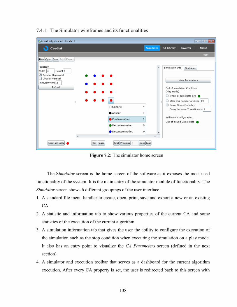
138
7.4.1. The Simulator wireframes and its functionalities
Figure 7.2: The simulator home screen
The Simulator screen is the home screen of the software as it exposes the most used
functionality of the system. It is the main entry of the simulator module of functionality. The
Simulator screen shows 6 different groupings of the user interface.
1. A standard file menu handler to create, open, print, save and export a new or an existing
CA.
2. A statistic and information tab to show various properties of the current CA and some
statistics of the execution of the current algorithm.
3. A simulation information tab that gives the user the ability to configure the execution of
the simulation such as the stop condition when executing the simulation on a play mode.
It also has an entry point to visualize the CA Parameters screen (defined in the next
section).
4. A simulator and execution toolbar that serves as a dashboard for the current algorithm
execution. After every CA property is set, the user is redirected back to this screen with

139
the CA being drawn in the drawing area. The user can execute the simulation by clicking
the "play" button. If needed, the user can use the step-by-step process by choosing the
appropriate buttons. The toolbar also offers utility tools such as the ability to reset the CA
with any desired state.
5. A topology screen that gives the user the opportunity to refresh the execution by altering
the topology, such as the size of the grid or the immunity time.
6. The drawing area itself located in the center of the software.
7.4.2. The CA Parameters wireframes and its functionalities
Figure 7.3: The CA parameters screen of the simulator module

140
The creation of a new CA and the editing of an existing CA will result in the opening
of the CA Parameters screen. In this user interface, the user will set (or update) all required
properties defining the CA (its name and description), its attributes (its width, its height, and
flags to check whether the algorithm to be defined acts on circular CA). The user also selects
the targeted neighbourhood from among the existing list of neighbourhood types saved in
the library. The user also specifies the decontamination characteristics such as the value of
the immunity time or the Contamination Distance, and of course, the Visibility Hop of the
CA.
One important function offered by this screen is the creation/update/removal of the
collection of transition rules associated with the CA. We take the decision to differentiate the
contamination rules (that is, the transition rules that lead a cell from a decontaminated state
into a contaminated one) among the other types of rules. The rationale is that contamination
rules can be dynamically generated by the system based on the type of neighbourhood, the
current Visibility Hop and the Contamination Distance (Algorithms for generating
contamination rules can be consulted in Appendix E). However, we still let the user initiate
the generation of contamination rules instead of relying on the system to automatically
initiate the rules. The reason for this is to give the user the control especially if the
previously mentioned parameters are updated.
Typically, after the contamination rules are generated, the user proceeds to
successively add the transition rules into the system. The configuration of the neighbourhood
will be constructed appropriately and the user just needs to select the correct cell state for the
current state, the result state, and the list of coherent states among the neighbourhood. By
default, all neighbour states are set to a "generic" value which can be altered with a specific
value. When the user finishes entering the input, the system will perform the validation of
the transition rules and show the Rules Validation Results screen.

141
7.4.3. The Inverter wireframes and its functionalities
Figure 7.4: The inverter home screen
The Inverter screen is the entry point of the Inverter module. The user interface has a
slight resemblance to the Simulator screen but has different purposes. The Inverter screen
shows six different groupings of the user interface.
1. A toolbar that serves as a dashboard for the Inverter process. It allows the user to create a
new inverter execution via the classic "new" button which will then open the Inverter
Parameter screen. After all parameters have been set, the user is directed back to this
screen with the CA generated on the drawing area. The user then selects the candidate
cells that are in a decontaminating state for each specific step. Meanwhile, at each step,
the system validates that the rules to be created do not invalidate the existing rules saved
to date. If there are conflicts, the system will display the errors through the Rules
Validation Results screen. At any time, the user can consult the list of rules already
created up to the current point. At his discretion, the user can indicate the end of the
entries’ capture and proceed to the recording of the generated rules. One key point is that

142
the generated rules are stored in the same database that store the transition rules for the
simulator module and therefore, the user can validate the algorithm by executing it
through the Simulator module.
2. A statistic and information tab to show various properties of the current execution and
some up to date statistics.
3. A simulation information tab that gives the user the ability to configure the execution of
the simulation. For instance, the user can configure the desired state of the cells outside
the boundary of the CA. The user can arrange to automatically set a decontaminating state
into decontaminated in the next step, if desired. This tab also has an entry point to
visualize the Inverter Parameters screen (defined in the next section).
4. A simulator and execution toolbar that serves as a dashboard for the current algorithm
execution. After the software successfully validates the transition rules, the user executes
the process by clicking the "play" button in the simulator and execution tool. If needed,
the user can use the step-by-step process by choosing the appropriate buttons.
5. A topology screen that gives the user the opportunity to refresh the execution by altering
the topology such as the size of the grid or the immunity time.
6. The drawing area itself located in the middle area of the software.

143
7.4.4. The Inverter-Parameter wireframes and its functionalities
Figure 7.5: The CA parameter screen of the inverter module
The creation of a new Inverter process and the editing of the CA’s current parameters
of the execution will result in the opening of the Inverter Parameter screen. In this user
interface, similar to the CA Parameter screen, the user will set all required properties
defining the current CA. The key difference between these two parameter screens (and the
backend functionality) is that in the CA Screen transition rules are added manually by the
user, while in the Inverter process, transition rules are generated by the system (the Inverter
algorithm) and these rules are only consulted on a read-only basis.
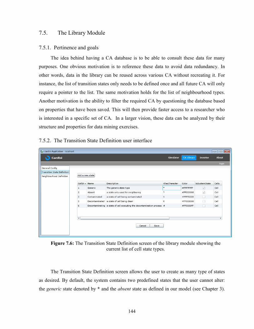
144
7.5. The Library Module
7.5.1. Pertinence and goals
The idea behind having a CA database is to be able to consult these data for many
purposes. One obvious motivation is to reference these data to avoid data redundancy. In
other words, data in the library can be reused across various CA without recreating it. For
instance, the list of transition states only needs to be defined once and all future CA will only
require a pointer to the list. The same motivation holds for the list of neighbourhood types.
Another motivation is the ability to filter the required CA by questioning the database based
on properties that have been saved. This will then provide faster access to a researcher who
is interested in a specific set of CA. In a larger vision, these data can be analyzed by their
structure and properties for data mining exercises.
7.5.2. The Transition State Definition user interface
Figure 7.6: The Transition State Definition screen of the library module showing the
current list of cell state types.
The Transition State Definition screen allows the user to create as many type of states
as desired. By default, the system contains two predefined states that the user cannot alter:
the generic state denoted by * and the absent state as defined in our model (see Chapter 3).

145
The user can create three states: contaminated, decontaminated and decontaminating if the
software is used for a Network Decontamination investigation. The user can also associate a
color and a character for each state. The color will serve to differentiate each cell during the
decontamination process. However, the character can be used if the user wishes to define the
rule using the traditional notation (see upcoming screen for the ruled definition)
7.5.3. The Neighbourhood Definition user interface
Figure 7.7: The Neighbourhood Definition edit screen of the library module showing
how to create a new type of neighbouhood
The neighbourhood definition tool allows the user to define a new type of
neighbourhood that he intends to use. By default, the system contains the von Neumann and
Moore neighbourhood. The collection of pre-saved neighbourhood types can later be
associated to the desired CA.

146
7.6. The Model
Figure 7.8: the data entity model of CAEDISI
The entity data model is a set of concepts that describe the structure of the data
regardless of its stored form. The conceptual model of the system is represented in the above
figure showing the data as entities and the relationships between these data.
The main entity of the system is the CellularAutomata object. Its name and
description helps the user for identification on a future use. It is also defined with an Id that
serves to key the object inside the database. Rather than just being considered a grid with a
width and a height, the CellularAutomata object is the root object of the system responsible

147
for materializing a specific algorithm. Therefore, it contains some particulars of the topology
such as Boolean values that identify for example if the CA is circular.
The CellularAutomata object is characterized by a single NeighbourhoodType
attribute. A NeighbourhoodType object is defined by the presence/absence of the cells
around it. For instance, the von Neumann neighbourhood has the flags IsTopOn, IsRightON,
IsBottomOn and IsLeftOn set to true and the remaining flags set to false.
A CellularAutomata is composed of several Cell objects whose number is the product
of the CellularAutomata's Width and its Height. Each Cell is equipped with coordinates
which indicate its position within the grid. Note that the entity data model stipulates that the
Cell is defined in 3D, but the current implementation only supports a 2D dimension.
Additionally, each Cell is provided with a description and a label which by default is the
concatenation of its coordinates itself (e.g., the label value of the cell at the top-left corner of
the CA is [0,0,0]). The user can alter these values as needed. For convenience, each Cell also
has a reference to its surrounding neighbours.
Each cell is characterized by a CellStateType, which can be a specific transition state
(contaminated, decontaminating, or decontaminated), an abstract state transition (e.g.,
generic and may represent any transition state), or just a qualification that expresses the
existential state of a cell (e.g., absent and therefore the cell is not present within the grid).
The generic type is only used in the expression of the definition of a transition rule while the
absent type is used simultaneously in the transition rules and in the grid when representing
sub-truncated CA. The idea of modeling an absent cell as a kind of transition state is
motivated by two reasons. Firstly, it facilitates the interpretation of the transition rules by
any algorithm, and secondly because an absent cell is seen by its neighbors as just a cell with
a particular state. The operation of representing a missing cell in the grid is identical to
changing the state of the cell.
A CellularAutomata object has a collection of TransitionRule objects assigned to it. A
TransitionRule object is defined by three criteria: the current cell state, the future cell state,
and the neighbourhood conditions of the current cell which specify the rules with respect to
transit from the current state to the future state. These neighborhood conditions are modeled
by a list of NeighbourhoodStateConfiguration objects.

148
A NeighbourhoodStateConfiguration object is a cell that only figures in the definition
of a neighbourhood. Thus, it has also a state. More importantly, its role is to be able to locate
itself relatively to the current cell to be transitioned. This is done through a coordinate
structure based on an offset. The use of an offset is motivated by the fact that the neighbour
cell can be present or missing within in the rule depending on the chosen neighborhood type
and the Visibility Hop.
7.7. The Simulator module
7.7.1. Pertinence and goals
The goal of simulation software is to be a tool to test and validate the feasibility of any
decontamination algorithm. Without simulation software, our algorithms would be tested on
paper. Unlike a traditional procedural algorithm, for which it is generally easy to find a
formal proof that the algorithm works optimally against certain criteria, it is often difficult to
simply show that an algorithm executed against a CA works as predicted. A procedural
algorithm is sequentially analyzed through its instructions; however, a CA algorithm runs in
a parallel fashion on each cell. Each cell may be subject to every transition rule depending
on its neighborhood at a given time t. Therefore on paper, each cell must be checked at each
stage to determine if it satisfies the neighborhood configuration of all recorded transitions’
rules. This may still be feasible in very simple conditions, for example in a small size CA of
visibility Vh=1 and equipped with a small neighborhood (e.g. von Neumann). However, the
same checking process would require considerable effort when the visibility increases (e.g.
Vh=3) and the neighborhood is large (e.g. Moore). In a simple algorithm, such as the basic
algorithm that decontaminates from left to right, cells can be classified into equivalence
classes with respect to their localization within the grid. When the flow decontamination is
not as regular, as in the Diagonal Snake, it becomes difficult or impossible to test the
algorithm on paper as there are many combinations of neighbourhood configuration during
the execution of the algorithm. Having software will not only save time in the testing of the
algorithms, but it can quickly provide an output and can offer a counter example of
neighbourhood configuration when the algorithm fails.

149
7.7.2. Application logic
The purpose of the simulation process is to sequentially produce the contents of a
dictionary whose key is a pair composed by the cell Id and the current step of execution t.
The value referenced by the key is an object containing the value of the cell state, the
immunity value at step t, and additional metadata that we will discuss in the next subsection.
To produce the contents of the dictionary, the algorithm relies on the CA data modeled on
the structure described in the entity model. The dictionary contents are consumed by the UI
with O(1) operation for each cell at any time t. The implementation of the main algorithm
can be consulted in Appendix A.
7.7.3. Simulation Metadata
Figure 7.9: A sample view of the metadata screen of the simulation module

150
The advantage of having simulation software is the ability to add features that provide
additional data generated by the execution. For example, within the data structure of the
simulation, we added a feature that allows the user to identify the exact rule that permits the
cell to pass into its new state. This additional information is shown in the figure above
(Figure 7.9) which illustrates the potential to have information regarding a cell at any given
time. In this example, during the Diagonal Snake algorithm, the user right-clicks on the cell
located in the first row and fourth column, and concludes that the rule R2 is responsible for
the transit of the cell (0, 3, 0) from contaminated to decontaminating. This feature gives a
confirmation of the status change, and it also allows us to access additional information such
as the value of the cell immunity (which is expected to decline at each step). A crucial
benefit is also the knowledge of when multiple rules are applicable for same cell and thus
could lead to a non-deterministic state of the cell in question.

151
7.8. Rules Validation & (Non) determinism
7.8.1. The transition rule collision validation
Figure 7.10: An example of two rules having collision errors
One condition that the software must validate is the presence of collision rules. Two or
more transition rules collide when they can target the same cell but the result state of these
elected rules are different (Figure 7.10). This means that the CA will face some non-
deterministic behaviour if the neighbourhood configurations referred to by the elected
transition rules are met during the execution.
When collisions are found during validation, the system displays a validation results
screen with all rules that collide. Then, it prompts the user to correct the issue (desired
behaviour) or to ignore the error messages and to assume the non-deterministic behaviour

152
(Figure 7.11). The implementation of the collision validation algorithm can be consulted in
Appendix D.
Figure 7.11: A view of the Rules Validation Results screen showing collision errors

153
7.8.2. The transition rule inclusion validation
Figure 7.12: An example of two rules having inclusion errors
Another condition that the software must also validate is the presence of inclusion
rules. Inclusion errors happen when there are multiple transition rules with identical result
states targeting the same cell (Figure 7.12). Unlike collision rules in which the software must
react with rejections, the system only needs to warn the user in the case of inclusion errors.
In most cases, this situation happens because of the use of the "generic" state when
expressing the state value of a cell during the transition rule definition. Unlike collision
rules, inclusion rules do not harm the system with a possibility of non-deterministic
behaviour. However, inclusion rules have an impact on the software performance because
the system will perform additional and unnecessary operations when evaluating a rule which
is already expressed by another existing rule.

154
When inclusion rules are found during validation, the system displays a validation
results screen with all rules that collide. Then, it prompts the user to correct the issue
(desired behaviour) or to ignore the error messages (Figure 7.13). The implementation of the
inclusion validation algorithm can be consulted in Appendix D.
Figure 7.13: A view of the Rules Validation Results screen showing inclusion errors
7.8.3. Validation Rules algorithm
Clearly, both inclusion and collision validation algorithms has to compare each pair of
saved rules. In the case of the collision rule validation, the first check is to verify if the
result state is different. However, in the inclusion rule, the result state has to be identical. In

155
both cases, the second step is to verify if the current neighbourhood configuration are
isomorphic with the pseudo-code below:
__________________________________________________________________________
Procedure boolean IsInputIsomorphic(
TransitionRule t1,
TransitionRule t2)
begin
For each NeighbourhoodStateConfiguration Nt1 in t1
If state of Nt1 *
begin
Nt2 the equivalent NeighbourhoodStateConfiguration in t2
If Nt2 and
state of Nt2 * and
state of Nt1 state of Nt2
begin
Return false
end
end
Return true
End
__________________________________________________________________________
In the case of collision rule, the input configuration is isomorphic and the result state is
different. In the case of inclustion rule, the input configuration is also isomorphic but the
result state is identical. Since the IsInputIsomorphic is done with O(1) operation (the
cardinality of NeighbourhoodStateConfiguration is constant as to the number neighbours is
fixed), both validation test executes in O(n2) in worst case as each pair of validation rules has
to be tested with n being the number of transition rules saved within the system. Both
implementation can be seen in [R13] with the procedure name
ValidateTransitionRulesInclusion and ValidateTransitionRuleCollision.
7.9. The Inverter module
7.9.1. Pertinence and goals
The Inverter module is the second major feature of the software and can be seen as an
inversion of the simulation process. At each stage, the user chooses the candidate cells for
being decontaminating and the system successively tries to recreate the transition rules. The
main motivation was to be able to quickly validate the feasibility of an idea for
156
decontamination through the stages of execution. If successful, the system would then be
responsible for generating the rules of decontamination. One advantage is that after the
generation of the rules, the user can revalidate the transition rules using the simulation
module. In the case of unfeasibility, the system would show a counter-example by
displaying a specific situation that contradicts the execution.
It is worth mentioning that unfeasibility is not fatal because it is possible that while the
decontamination idea does not work within the parameters entered, it might still be possible
with other parameters. As we have seen in Chapter 6, the diagonal snake algorithm is
unfeasible with von Neumann of visibility Vh=2 but is feasible with von Neumann of
visibility Vh=3 or in the vicinity of Moore visibility Vh=2. Fortunately, the software allows
the user to use the Inverter module by varying different parameters such as visibility,
neighborhood, and immunity. Under this approach, the software can be used as a research
tool by helping the researcher to understand the dynamics of the decontamination strategy
and the influence of the CA properties.
7.9.2. Application logic
The purpose of the inverter algorithm is to create the collection of transition rules
generated by the Inverter. The Figure 7.14 below shows the execution of the Inverter and the
content of the transition rules during a recreation of the diagonal move algorithm on a CA of
Vh=1, Cd=1 and It=0. At the initial stage, only the contamination rules are contained in the
TransitionRules object (Figure 7.14a). The user initiates the Inverter process by selecting the
first decontaminating cell (at position [0,0]) at step t=0 (Figure 7.14b), Then, the user
commands the system to store and validate this data, which automatically sets the cell [0,0]
to decontaminated at step t=1. The user sets both cells at position [0,1] and [1,0] to a
decontaminating state (Figure 7.14c). The user then commands the system again to move to
the next step t=2. At this stage, the TransitionRules object will add the last 3 rules displayed
in Figure 7.14d. The implementation of the main Inverter algorithm can be consulted in
Appendix B (with Immunity) and Appendix C(without Immunity).

157
(b) (c)
(a) (d)
Figure 7.14: An example of the Inverter execution showing the creation of rules
Unlike the simulation module where a specific data structure is needed to hold each
cell state at each step, the Inverter process does not necessarily rely on only one unique data
structure. As data storage, we actually use the CA object as specified in the entity data
model to store the inverter parameters. The collection rules are also stored in its
TransitionRule child object. In order to support a preview of the pre-entered data (with the
forward and backward buttons) for the user to re-verify his entry, we use the same type of
dictionary used by the simulation module. Once the user has decided the value of each

158
parameter defining the CA, the size of the latter is static and fixed during each execution.
Therefore, a regular array is used as a temporary data structure to store the state of each CA
at each step. Transition rules are built based on the contents of the previous and the current
step arrays.
7.9.3. Miscellaneous notes
(a) (b) (c)
(d) (e) (f)
Figure 7.15: The impact of an even/odd sized CA on the Inverter
It is important to note that the performance of the inverter only takes into account the
"exact" neighborhood during the construction of each transition rule. (Indeed, the software is
not trying to create rules using generic state). As noted in the previous chapter, there are
some cases in which created rules still require intervention in order to work for any size of
CA. The diagonal snake algorithm, whose rules generated by the execution of the Inverter on
a CA with an even size, could not be directly generalized to any size n and moreover, the
generalization is not trivial.

159
The same situation is encountered when we look at the example of using the inverter to
generate the rules of the diagonal move approach. In this scenario, we see that the
generalization can be done easily. Take the example shown in the previous figure where the
rules were generated by running the inverter algorithm on a CA of an odd size. When
executing the inverter for n = 5, we note that decontamination performs as expected (Figures
(a) , (b) and (c)). However, when executing the rules against a CA of an even size, we notice
some runtime defects as shown in Figure (f) because the cells pointed to by the arrows
should be in a decontaminated state in stage (f). The reason is that the configuration of the
stage shown in Figure (e) has never been treated during the execution. We do not find the
configuration of Figure (e) in (a), nor (b) and (c). To fix the issues, we can add the simple
rule . With this addition, we end up with a set of rules which
work with both even and odd sized CA.

160
Chapter 8
8. Summary & Future work
In this chapter, we summarize the work that we have completed so far. We discuss possible
directions for future work based on the solutions that we have proposed, and we also discuss
some new ideas.
8.1. Summary
In this thesis, we have studied the decontamination in CA through two new additional
concepts: Visibility Hop and Contamination Distance. Specifically, we have proposed
different solutions and evaluated these solutions according to the established complexity
measures. Our goal was to understand the impact of these two assumptions on existing
solutions. Then, we proposed new algorithms occasioned by these concepts.
In Chapter 2, we provided a survey of the current state of research in external and
internal Network Decontamination with a concentration on internal Network
Decontamination. We also briefly discussed CA. This survey helped by providing an in
depth understanding of the decontamination problem, and the different techniques useful in
our study of Network Decontamination problems.
In Chapter 3, we formally described the model used in this thesis: Network
Decontamination using CA under the new assumptions Visibility Hop and Contamination
Distance. Our model is a regular grid of cells, having three states (contaminated,
decontaminating, and decontaminated) and where the cells change their state synchronously
according to local rules. In our study, we also considered the notion of Time Immunity in
some cases.
In Chapters 4, 5 and 6, we have shown the pertinence of these two new parameters. In
Chapter 4, we analyzed known basic decontamination algorithms with different values for
Visibility Hop and Contamination Distance. We started by analyzing existing basic
algorithms under these new assumptions and we provided some solutions on how these
strategies can be updated to have better results.

161
In Chapter 5, we proposed new algorithms characterized by diagonal moves. We have
also shown that the use of Visibility Hop leads to better results when applied to our diagonal
algorithms, especially when considering the average number of decontaminating cells being
utilized. We gave a list of rules that accomplish the decontamination for specific values of
Cd and Vh. We also gave a general algorithm for any arbitrary values of these two
parameters.
In Chapter 6, we proposed some new ideas that can only be fulfilled if Visibility Hop
2Vh holds. We proposed two new algorithms called Road Traffic and Diagonal Snake,
and we indeed claim that they are only feasible if the CA allows greater visibility and
Immunity time. Initial results have shown improvement with respect to the decontamination
time and the maximum Immunity time when compared to existing algorithms. We have
shown that we can transpose these ideas and complement them with some divide-and-
conquer strategies by applying similar ideas against different locations within the CA. We
also studied the possibility of subdividing the execution by using the diagonal moves
introduced in Chapter 5.
In Chapter 7, we presented software that we implemented to support our study. Among
all functionalities, there are two key pieces. One is the software’s simulator module which
allows the user to enter any pre-defined list of decontamination rules and witness the
execution of the decontamination in a flexible manner. The other important functionality is
the software’s rules generator module which allows the software to generate some
decontamination rules based on a idea of an execution. The building of the tool was
essential because of the non existence of a tool that can take account of Visibility Hop,
Contamination Distance, and Time Immunity. The resulting software is a complete research
tool which can assist any researcher who focuses his work on CA, or Network
Decontamination under that structure.
8.2. Current work extension and Future work
There are several ways in which we propose to continue the work begun here.
In this thesis, we concentrated our effort on studying the CA model in which the
transition rules’ results are defined in a precise way, and as soon as a neighbourhood
configuration is met, the result state is final. We would like to investigate the case when the
162
result state is not necessarily fixed, but instead has a probabilistic factor of transiting to the
new defined state. We have inserted the code to support this behaviour within the software
but we would like to have a theoretical study of the possible stochastic models that are
meaningful for Network Decontamination. This model responds to a very realistic situation
in which some of the decontamination programs executed against the machine do not
automatically succeed. For instance, during the diagonal move process, what happens when
some of cells laying on the next diagonal do not necessarily transit to a decontaminating
state? Can the defined algorithm still perform? How are we to classify existing algorithms
which can positively react to this new input? Ultimately, we want to know how to build
classes of algorithms that are immune to these probabilistic factors.
In this thesis, we have assumed monotone strategies to decontaminate the network. We
would like to investigate the implementation of non-monotone strategies and the impact on
Time Immunity and recontamination. The study of Network Decontamination using CA with
non-monotone strategies is still very open and few results are known.
In this thesis, we assumed that the network is reliable, that is, the links and the nodes
are not broken. What happens when, for example, a node cannot receive the state of its
neighbour? What happens if the node sends the wrong state value to its neighbour? We gave
a brief introduction of the possible issues in Chapter 3. Undeniably, the addition of fault
tolerance in our algorithms is another attractive future work.
We also want to complement our software with new set of requirements. One evident
functionality is to add the support of Mobile agents, which has the most interest among
researchers in distributed computing. This will allow an experimental analysis of the impact
of Visibility Hop on the new model introduced in [DFZ11] called Mobile CA MCA, a CA
navigated by a Mobile Agent.
Finally, we intend to continue and finalize our research related to sub-truncated
networks. We want to know the largest sub-truncated mesh that decreases the number of
decontaminating cells. We expect that the understanding of the problem of decontamination
in a sub network with fewer hosts, yet close enough to the full network, will allow us to find
different perspectives on a new decontamination algorithm. We present a brief explanation
of the problem.
163
Problem definition. Assume an optimal decontaminating strategy requires p simultaneously
decontaminating cells to decontaminate a n*m 2D mesh. The goal is to identify the
minimum number of cells x to be removed from the topology in order to decontaminate the
newly sub-truncated network with a predefined k (with k<p) simultaneously decontaminating
cells at any time t. The goal may also be to identify the maximum number of cells k which
can be added to the topology without increasing the p simultaneously decontaminating cells.
We believe that the research tool we have developed can offer us significant support during
our exploration.
164
Bibliography
[ADF07] L. Acerbi, A. Dennunzio, E. Formenti. Shifting and lifting of CA. In
Proceedings of the 3rd conference on Computability in Europe: Computation
and Logic in the Real World, pages 1-10, Berlin, Heidelberg, 2007.
[ADF09] L. Acerbi, A. Dennunzio, E. Formenti. Conservation of some dynamical
properties for operations on CA. Theor. Comput. Sci.,410:3685-3693, 2009.
[Als04] B. Alspach, Searching and sweeping graphs: a brief survey, International
Conference in Combinatorics, Le Matematiche, Vol LIX - Fasc. I-II, pp. 5–37,
2004.
[Awa08] A. Awazu, Input-dependent wave propagations in asymmetric CA: possible
behaviors of feed-forward loop in biological reaction network, Mathematical
Biosciences and Engineering, Volume 5, Issue 3, 419 - 427, 2008.
[BFFS02] L. Barrière, P Flocchini, P. Fraigniaud, and N. Santoro. Capture of an Intruder
by Mobile Agents. In ACM Symposium on Parallelism in Algorithms and
Architectures (SPAA), pages 200-209, 2002.
[Bre67] R. Breisch., An intuitive approach to speleotopology, Southwestern Cavers,
vol. VI, no. 5, pp. 72-78, 1967.
[CD98] B. Chopard and M. Droz. CA Modeling of Physical Systems, Cambridge
University Press, 1998.
[Cel88] CelLab, http://www.fourmilab.ch/cellab/, online.
[Daa12] Y. Daadaa. Network Decontamination with Temporal Immunity, phd Thesis,
University of Ottawa, Ottawa, Ontario, Canada, 2012.
[DFZ10] Y. Daada, P. Flocchini, N. Zaguia. Network Decontamination with temporal
immunity by CA, 9th Int. Conference on CA for Research and Industry
(ACRI), 287-299, 2010
[DFZ11] Y. Daadaa, P. Flocchini, N. Zaguia, Decontamination with Temporal Immunity
by Mobile CA, In proceeding of: 3rd annual CA Workshop (CSC), 2011.
[DLFM09] A. Dennunzio, P .Di Lena, E .Formenti, and L. Margara. On the Directional
Dynamics of Additive CA. Theoretical Computer Science, 410:4823-4833,
2009.
165
[EF08] Entity Framework, http://www.asp.net/entity-framework, online.
[FHL06] P. Flocchini, M.J. Huang, F.L. Luccio., Decontamination of chordal rings and
Tori, Proc. 8th Workshop on Advances in Parallel and Distributed
Computational, 2006.
[FHL07] P. Flocchini, M.J. Huang , F.L. Luccio. Decontamination of chordal rings and
tori using mobile agents. International Journal of Foundation of Computer
Science, 18(3), 547-564, 2007
[FHL08] P. Flocchini, M.J. Huang, F.L. Luccio. Decontamination of hypercubes by
mobile agents, Networks, 52(3): 167-178, 2008
[FIP+05] P. Fraigniaud, D. Ilcinkas, G. Peer, A. Pelc, and D. Peleg. Graph Exploration
by a Finite Automata. Theoretical Computer Science, 345(2-3):331-344, 2005.
[Flo09] P. Flocchini. Contamination and decontamination in majority-based
systems, Journal of CA, 4(3):183-200, 2009.
[Fia01] FiatLux, http://webloria.loria.fr/~fates/FiatLux/presentation-fr.html, online.
[FLPS13] P. Flocchini, F. Luccio, L. Pagli, N. Santoro, Optimal Network
Decontamination with threshold immunity, 8th International Conference on
Algorithms and Complexity (CIAC), 2013.
[FMS08] P. Flocchini, B. Mans, and N. Santoro. Tree Decontamination with Temporary
Immunity. In 19th International Symposium on Algorithms and Computation
(ISAAC), pages 330-341, 2008.
[FNS05] P. Flocchini, A. Nayak, and A. Schulz. Cleaning an Arbitrary Regular Network
with Mobile Agents. In 2nd International Conference Distributed Computing
and Internet Technology (ICDCIT), pages 132-142, 2005.
[Gar70] M. Gardner. The Fantastic Combinations of John Conway's New Solitaire
Game "Life". Sci. Am., 223:120-123, 1970.
[Gol00] Golly, http://golly.sourceforge.net/, online.
[JCA00] JCASim: CA simulation system, http://www.jcasim.de/, online.
[Kar05] J. Kari, Theory of CA: A survey, Theoretical Computer Science, Volume 334,
Issues 1–3, Pages 3–33, April 2005.
[Kar90] J. Kari, Reversibility of 2D CA is undecidable, Physica D: Nonlinear
Phenomena, Volume 45, Issues 1–3, Pages 379–385, 1990.

166
[KK07] E. Kranakis, D. Krizanc. An Algorithmic Theory of Mobile Agents, In
proceedings of TGC 2006, 2nd Symposium on Trustworthy Global Computing,
Lucca, Italy, 2007.
[KP00] S. Kutten, D.Peleg. Tight Fault locality. SIAM Journal on Computing, 30:247-
268, 2000.
[KVZ09] J. Kari, P. Vanier, and T. Zeume. Bounds on Non-Surjective CA. In 34th
International Symposium on Mathematical Foundations of Computer Science
(MFCS), 439-450, 2009.
[Lap93] A. S. LaPaugh. Recontamination Does Not Help to Search a Graph. Journal of
the ACM, 40(2):224-245, 1993.
[LM08] P. di Lena and L. Margara. Computational Complexity of Dynamical Systems:
The Case of CA. Information and Computation, 206(9-10):1104-1116, 2008.
[LM10] P. di Lena, L. Margara. On the Undecidability of the Limit Behavior of CA,
Theoretical Computer Science, 411(7-9), 1075-1084, 2010.
[LP09] F. Luccio, Linda Pagli. A general approach to toroidal mesh decontamination
with local immunity. In Proceedings of the 2009 IEEE International
Symposium on Parallel & Distributed Processing (IPDPS '09). IEEE
Computer Society, 1-8, 2009.
[LPS06] F. Luccio, L. Pagli, N. Santoro. Network Decontamination with local
immunization. In Proceedings of the 20th international conference on Parallel
and distributed processing (IPDPS'06), 2006
[LPS07] F. Luccio, L. Pagli, N. Santoro, Network Decontamination in presence of local
immunity, Int. Journal of Foundations of Computer Science, 18 (3): 457-474,
2007
[Mce99] MCell, http://www.mirekw.com/ca/index.html, online.
[Mes08] M.-E. Messinger, Methods of Decontaminating Networks, Phd Thesis,
Dalhousie University, Halifax, Nova Scotia, Canada, 2008.
[MHG+88] N. Megiddo, S. Hakimi, M. Garey, D. Johnson, and C. Papadimitriou. The
complexity of searching a graph. Journal of the ACM, 35(1):18–44, 1988.
[MG68] E. F. Moore, G. G. Langdon. A generalized firing squad problem, Information
and Control 12 (3), 212–220, 1968.
[Mit96] M. Mitchel, Computation in CA: A Selected Review, Technical Report, Santa
Fe Institute, New Mexico, 1996.

167
[Neu51] J. v. Neumann, The general and logical theory of automata, L.A. Jeffress, ed.,
Cerebral Mechanisms in Behavior – The Hixon Symposium, John Wiley &
Sons, New York, pp. 1-31, 1951.
[Neu96] J.v.Neumann, theory of self-reproducing automata, Univ. of Illinois, Urbana
1996.
[Pac86] N. H. Packard. Lattice Models for Solidification and Aggregation. In First
International Symosium for Science on Form, 1986.
[Par76] T. D. Parsons, Pursuit-evasion in a graph. Theory and Applications of Graphs.
Springer-Verlag. pp. 426–441, 1976.
[Par78] T. D. Parsons. The Search Number of a Connected Graph. In 9th Southeastern
Conference on Combinatorics, Graph Theory and Computing, Utilitas
Mathematica, pages 549-554, 1978.
[Pel02] D. Peleg. Local majority voting, small coalitions and controlling monopolies in
graphs: A review. Theoretical Computer Science 282, 231–257, 2002.
[Qiu07] J. Qiu. Best Effort Decontamination of Networks. Master's thesis, University
of Ottawa, 2007
[R13] L. Rakotomalala, Caedisi source code, https://caedisi.codeplex.com/, online.
[RZ15] L. Rakotomalala, N. Zaguia, CAEDISI: A Cellular Automata Editor and
Simulator for Network Decontamination, The society for Modeling and
Simulation International, SummerSim’15 (SCSC2015), Chicago, IL, USA,
2015.
[Sab08] M. Sablik. Directional Dynamics for CA: a Sensitivity to Initial Condition
Approach. Theoretical Computer Science, 400(1-3):1-18, 2008.
[Sch02] B. Schonfisch. Propagation of Fronts in CA. Physica D, 80:433-450, October
2002.
[Sil10] Silverlight, http://www.microsoft.com/silverlight/, online.
[SQL05] SQL Server, http://www.microsoft.com/sql, online.
[WCF04] WCF RIA Services, http://msdn.microsoft.com/en-
us/library/ee707344(v=vs.91).aspx, online.
[WMS88] Wolfram Mathematica Software, http://wolfram.com/, online
[Wol84] S. Wolfram. Universality and complexity in CA, Physica D: Nonlinear
Phenomena, Volume 10, Issues 1–2, 1–35, 1984.

168
[Wol88] S. Wolfram. High Speed Computing, Scientific Application and Algorithm
Design, ed. Robert B. Wilhelmson. University of Illinois Press, 1988.
[Wol94] S. Wolfram. Theory and Applications of CA, World Scientific (1986), CA and
Complexity, Addison-Wesley, Massachusetts, 1994.
[Wol02] Stephen Wolfram, A new kind of science, Wolfram Media, 2002.

169
Appendix A: Implementation of the Simulation algorithm
/// <summary>/// Processes the transition rules algorithm. The goal is to produce new state for each cell of the cellular automata /// based on which transition rules is eligible applied to that cell. The data structure that holds the state for each/// step is the SystemStateDictionary. /// </summary>/// <param name="cellularAutomata">The cellular automata.</param>/// <param name="newStep">The new step.</param>private void ProcessTransitionRulesAlgorithm(Web.DataModel.CellularAutomata cellularAutomata, int newStep){ int numberOfRows = cellularAutomata.Height; int numberOfColumns = cellularAutomata.Width;
for (int i = 0; i < numberOfRows; i++) { for (int j = 0; j < numberOfColumns; j++) { int k = 0; // only 2D for now Cell myCell = cellularAutomata.CellularAutomataAsArray[i, j, k]; SimulationIterationItem previousIterationItem = GetSimulationIterationItem(myCell.CellId, newStep-1, false); SimulationIterationItem newIterationItem = GetSimulationIterationItem(myCell.CellId, newStep, true); newIterationItem.Reset();
//grab which rules applies to myCell foreach (TransitionRule rule in cellularAutomata.TransitionRules) { bool doesCellCurrentStateSatisfyRule = DoesCellConfigurationSatisfyTransitionRule(myCell, rule, cellularAutomata); if (doesCellCurrentStateSatisfyRule) newIterationItem.TransitionRulesCause.Add(rule); } //by default, the result state is the old value int resultCellStateTypeId = myCell.CellStateTypeId; if (newIterationItem.TransitionRulesCause.Count > 0) { if (newIterationItem.IsDeterministic) { int tentativeResultCellStateTypeId = newIterationItem.TransitionRulesCause.First().ResultCellStateTypeId; if (tentativeResultCellStateTypeId == ((int)EnumCellStateType.Decontaminated)) { resultCellStateTypeId = ((int)EnumCellStateType.Decontaminated); //each time the cell gets decontaminated (i.e the virus has been cleant), //the immunity timer is reset newIterationItem.ImmunityTimerValue = cellularAutomata.ImmunityTime; } else if (tentativeResultCellStateTypeId == ((int)EnumCellStateType.Contaminated)) { //it will goes to contaminated if the cell is no more immune if (previousIterationItem == null || previousIterationItem.ImmunityTimerValue == 0) { resultCellStateTypeId = ((int)EnumCellStateType.Contaminated); } else resultCellStateTypeId = myCell.CellStateTypeId; //decrease the timer newIterationItem.ImmunityTimerValue = (previousIterationItem.ImmunityTimerValue > 0 ? previousIterationItem.ImmunityTimerValue - 1 : 0); } else resultCellStateTypeId = tentativeResultCellStateTypeId; }

170
else { // Undeterministic (We found multiple transition rules that can be applied to the // cells but their result state are different) The Code decision is to keep the previous // transition result but we flag that the cell has an issue resultCellStateTypeId = myCell.CellStateTypeId; //even for underterministic case, we still decrease the immunity timer when the previous //state has a timer value set if (previousIterationItem.CellStateTypeId == ((int)EnumCellStateType.Decontaminated)) newIterationItem.ImmunityTimerValue = (previousIterationItem.ImmunityTimerValue > 0 ? previousIterationItem.ImmunityTimerValue - 1 : 0); } } else { if (resultCellStateTypeId == ((int)EnumCellStateType.Decontaminated)) { newIterationItem.ImmunityTimerValue = (previousIterationItem.ImmunityTimerValue>0 ? previousIterationItem.ImmunityTimerValue-1 : 0); } } //setting the final result state newIterationItem.CellStateTypeId = resultCellStateTypeId;
Tuple<Guid, int> newIterationItemKey= new Tuple<Guid,int>(myCell.CellId, newStep); this.SystemStateDictionary[newIterationItemKey] = newIterationItem; } }}

171
Appendix B: Implementation of the Inverter (without immunity) algorithm
private void ValidateAndStoreStatesNoImmunity(InverterExecution currentInverterExecution, Collection<RuleValidationError> validationResultsCollisionRules){ int currentStep = currentInverterExecution.CurrentStep; int previousStep = currentInverterExecution.CurrentStep - 1;
int numberOfRows = currentInverterExecution.CellularAutomata.Height; ; int numberOfColumns = currentInverterExecution.CellularAutomata.Width;
InvertedCellItem[, ,] previousCellularAutomataAsArrayInvertedCellItem = currentInverterExecution.TemporalCellularAutomata[previousStep];
//foreach (Cell cell in this.CurrentCellularAutomata.Cells) for (int i = 0; i < numberOfRows; i++) { for (int j = 0; j < numberOfColumns; j++) { Cell myCell = currentInverterExecution.CellularAutomata.CellularAutomataAsArray[i, j, 0]; int currentCellStateTypeId = myCell.CellStateTypeId;
//get the previousCellStateTypeId int previousCellStateTypeId =
previousCellularAutomataAsArrayInvertedCellItem[i, j, 0].CellStateTypeId;
//build the transition Rule TransitionRule newTransitionRule = EntityHelper.GenerateGenericTransitionRule( "([" + i + "," + j + "]|" + previousStep + "->" + currentStep + ") ", string.Empty, currentInverterExecution.CellularAutomata.NeighbourhoodTypeId, currentInverterExecution.CellularAutomata.RadiusVisibility);
newTransitionRule.CurrentCellStateTypeId = previousCellStateTypeId; newTransitionRule.ResultCellStateTypeId = currentCellStateTypeId; //even though it is system generated, it is still simulating a user created. newTransitionRule.IsSystemGenerated = false; //now set the neighbourhood foreach (NeighbourhoodStateConfiguration ruleStateConfiguration
in newTransitionRule.NeighbourhoodStateConfigurations) { ruleStateConfiguration.CellStateTypeId = EntityHelper.GetNeighbourCellStateTypeId( myCell, previousCellularAutomataAsArrayInvertedCellItem, ruleStateConfiguration, currentInverterExecution.CellularAutomata.CircularVertical, currentInverterExecution.CellularAutomata.CircularHorizontal, currentInverterExecution.OutOfBoundCellStateTypeId); }

172
//validate the new rule bool hasInclusion = false; bool hasCollision = false; foreach (TransitionRule existingRule in currentInverterExecution.CellularAutomata.TransitionRules) { if (newTransitionRule.CurrentCellStateTypeId == existingRule.CurrentCellStateTypeId) { //inclusion if (newTransitionRule.ResultCellStateTypeId == existingRule.ResultCellStateTypeId && EntityHelper.IsInputIsomorphic(newTransitionRule, existingRule)) { hasInclusion = true; } //collision if (newTransitionRule.ResultCellStateTypeId != existingRule.ResultCellStateTypeId && EntityHelper.IsInputIsomorphic(newTransitionRule, existingRule)) { hasCollision = true; newTransitionRule.CellularAutomata = currentInverterExecution.CellularAutomata; validationResultsCollisionRules.Add(new RuleValidationError(newTransitionRule, existingRule)); } } }
if (!hasCollision && !hasInclusion) currentInverterExecution.CellularAutomata.TransitionRules.Add(newTransitionRule); }
}}

173
Appendix C: Implementation of the Inverter (with immunity) algorithm
private void ValidateAndStoreStatesWithImmunity(InverterExecution currentInverterExecution, Collection<RuleValidationError> validationResultsCollisionRules){ int currentStep = currentInverterExecution.CurrentStep; int previousStep = currentInverterExecution.CurrentStep - 1;
int numberOfRows = currentInverterExecution.CellularAutomata.Height; ; int numberOfColumns = currentInverterExecution.CellularAutomata.Width;
InvertedCellItem[, ,] previousCellularAutomataAsArrayInvertedCellItem = currentInverterExecution.TemporalCellularAutomata[previousStep];
//foreach (Cell cell in this.CurrentCellularAutomata.Cells) for (int i = 0; i < numberOfRows; i++) { for (int j = 0; j < numberOfColumns; j++) { Cell myCell = currentInverterExecution.CellularAutomata.CellularAutomataAsArray[i, j, 0]; int currentCellStateTypeId = myCell.CellStateTypeId;
if (currentCellStateTypeId == ((int)EnumCellStateType.Contaminated)) { ; //no need to perform as we explicity ignore immunity. } else { //get the previousCellStateTypeId int previousCellStateTypeId =
previousCellularAutomataAsArrayInvertedCellItem[i, j, 0].CellStateTypeId; //build the transition Rule TransitionRule newTransitionRule = EntityHelper.GenerateGenericTransitionRule( "([" + i + "," + j + "]|" + previousStep + "->" + currentStep + ") ", string.Empty, currentInverterExecution.CellularAutomata.NeighbourhoodTypeId, currentInverterExecution.CellularAutomata.RadiusVisibility);
newTransitionRule.CurrentCellStateTypeId = previousCellStateTypeId; newTransitionRule.ResultCellStateTypeId = currentCellStateTypeId; //even though it is system generated, it is still simulating a user created. newTransitionRule.IsSystemGenerated = false; //now set the neighbourhood foreach (NeighbourhoodStateConfiguration ruleStateConfiguration
in newTransitionRule.NeighbourhoodStateConfigurations) { ruleStateConfiguration.CellStateTypeId = EntityHelper.GetNeighbourCellStateTypeId( myCell, previousCellularAutomataAsArrayInvertedCellItem, ruleStateConfiguration, currentInverterExecution.CellularAutomata.CircularVertical, currentInverterExecution.CellularAutomata.CircularHorizontal, currentInverterExecution.OutOfBoundCellStateTypeId); }

174
//validate the new rule bool hasInclusion = false; bool hasCollision = false; foreach (TransitionRule existingRule
in currentInverterExecution.CellularAutomata.TransitionRules) { if (newTransitionRule.CurrentCellStateTypeId == existingRule.CurrentCellStateTypeId) { //inclusion if (newTransitionRule.ResultCellStateTypeId == existingRule.ResultCellStateTypeId && EntityHelper.IsInputIsomorphic(newTransitionRule, existingRule)) { hasInclusion = true; } //collision if (newTransitionRule.ResultCellStateTypeId != existingRule.ResultCellStateTypeId && EntityHelper.IsInputIsomorphic(newTransitionRule, existingRule)) { if (existingRule.ResultCellStateTypeId == ((int)EnumCellStateType.Contaminated) && newTransitionRule.ResultCellStateTypeId == ((int)EnumCellStateType.Decontaminated)) { if (previousCellularAutomataAsArrayInvertedCellItem[i, j, 0].ImmunityTimerValue == 0) { hasCollision = true; newTransitionRule.CellularAutomata = currentInverterExecution.CellularAutomata; validationResultsCollisionRules.Add(new RuleValidationError(newTransitionRule, existingRule)); } else { ; //no collision, protected by immunity } } else { hasCollision = true; newTransitionRule.CellularAutomata = currentInverterExecution.CellularAutomata; validationResultsCollisionRules.Add(new RuleValidationError(newTransitionRule, existingRule)); } } } } if (!hasCollision && !hasInclusion) currentInverterExecution.CellularAutomata.TransitionRules.Add(newTransitionRule); } } }}

175
Appendix D: Implementation of the rules collision/inclusion validation
algorithm public static Collection<RuleValidationError> ValidateTransitionRulesCollision(CellularAutomata cellularAutomata){ Collection<RuleValidationError> result = new Collection<RuleValidationError>(); int size = cellularAutomata.TransitionRules.Count;
for (int i = 0; i < size; i++) { TransitionRule t1 = cellularAutomata.TransitionRules.ElementAt(i); for (int j = i + 1; j < size; j++) { TransitionRule t2 = cellularAutomata.TransitionRules.ElementAt(j); // A collision occurs between 2 rules when their current state is the same, their resulting state are different // however the input neighbourhood configuration are similar if (t1.CurrentCellStateTypeId == t2.CurrentCellStateTypeId && t1.ResultCellStateTypeId != t2.ResultCellStateTypeId) { //validate if the input are the same. bool isInputIsomorphic = IsInputIsomorphic(t1, t2); if (isInputIsomorphic) result.Add(new RuleValidationError(t1, t2)); } } } return result;}
public static Collection<RuleValidationError> ValidateTransitionRulesInclusion(CellularAutomata cellularAutomata){ Collection<RuleValidationError> result = new Collection<RuleValidationError>(); int size = cellularAutomata.TransitionRules.Count;
for (int i = 0; i < size; i++) { TransitionRule t1 = cellularAutomata.TransitionRules.ElementAt(i); for (int j = i + 1; j < size; j++) { TransitionRule t2 = cellularAutomata.TransitionRules.ElementAt(j); // An inclusion occurs between 2 rules if their current state are the same , their resulting state is the same, // and the neighbourhood configuration neighbourhood configuration are similar or one is contained in another if (//!t1.IsSystemGenerated && !t2.IsSystemGenerated && t1 != t2 && t1.CurrentCellStateTypeId == t2.CurrentCellStateTypeId && t1.ResultCellStateTypeId == t2.ResultCellStateTypeId) { //validate if the input are the same. bool isInputIsomorphic = IsInputIsomorphic(t1, t2); if (isInputIsomorphic) result.Add(new RuleValidationError(t1, t2)); } } } return result;}
public static bool IsInputIsomorphic(TransitionRule t1, TransitionRule t2){ bool isInputIsomorphic = true;
foreach (NeighbourhoodStateConfiguration t1Neighbour in t1.NeighbourhoodStateConfigurations) { if (t1Neighbour.CellStateTypeId != (int)EnumCellStateType.Generic) //no need to check if one is generic { NeighbourhoodStateConfiguration t2EquivalentNeighbour = t2.NeighbourhoodStateConfigurations.Where( neighbour => neighbour.x_offset == t1Neighbour.x_offset && neighbour.y_offset == t1Neighbour.y_offset && neighbour.z_offset == t1Neighbour.z_offset).SingleOrDefault(); if (t2EquivalentNeighbour != null && t2EquivalentNeighbour.CellStateTypeId != (int)EnumCellStateType.Generic && t1Neighbour.CellStateTypeId != t2EquivalentNeighbour.CellStateTypeId) { isInputIsomorphic = false; break; } } } return isInputIsomorphic;}

176
Appendix E: Implementation of the contamination rules generation algorithm
public static void GenerateContaminationRule(CellularAutomata cellularAutomata, NeighbourhoodType selectedNeighbourhoodType, ref int numberOfRulesCreated){ //using a temporary rule to loop through all existing neighbours TransitionRule tempRule = EntityHelper.GenerateGenericTransitionRule( string.Empty, string.Empty, selectedNeighbourhoodType, cellularAutomata.RadiusVisibility); //then create all contamination rule foreach (NeighbourhoodStateConfiguration configuration in tempRule.NeighbourhoodStateConfigurations) { //only generate when the contamination radius is smaller than the visibility radius if (configuration.DistanceFromCenter <= cellularAutomata.RadiusContamination) { numberOfRulesCreated++;
TransitionRule newContaminationRule = EntityHelper.GenerateGenericTransitionRule( "Rule #" + numberOfRulesCreated + " (Contamination)", "Contamination rule infecting a clean cell when a contaminated cell is located at a contamination radius=" + cellularAutomata.RadiusContamination + " and a visibility radius=" +cellularAutomata.RadiusVisibility, selectedNeighbourhoodType as NeighbourhoodType, cellularAutomata.RadiusVisibility);
newContaminationRule.CurrentCellStateTypeId = (int)EnumCellStateType.Decontaminated; newContaminationRule.ResultCellStateTypeId = (int)EnumCellStateType.Contaminated; newContaminationRule.IsSystemGenerated = true; NeighbourhoodStateConfiguration thisConfiguration =
newContaminationRule.NeighbourhoodStateConfigurations.Where(stateConfiguration => stateConfiguration.x_offset == configuration.x_offset
&& stateConfiguration.y_offset == configuration.y_offset && stateConfiguration.z_offset == configuration.z_offset).First(); //set this neighourhood to contaminated and leave the remaining neighbours as generic thisConfiguration.CellStateTypeId = (int)EnumCellStateType.Contaminated; cellularAutomata.TransitionRules.Add(newContaminationRule); } } }
public static TransitionRule GenerateGenericTransitionRule(string name, string description, NeighbourhoodType neighbourhoodType, int radiusVisibility){ TransitionRule transitionRule = new TransitionRule() { Name = name, Description = description }; int minOffset = radiusVisibility * (-1); int maxOffset = radiusVisibility * (1); int xIndexCenterCell = maxOffset; int yIndexCenterCell = maxOffset; int zIndexCenterCell = 0; //for now we only deal with 2D //Generate recursively the neighbouring cells data according to the neighbourhoodtype int currentRadiusIndex = 0; EntityHelper.GenerateListNeighboursData(transitionRule, xIndexCenterCell, yIndexCenterCell, zIndexCenterCell, neighbourhoodType, currentRadiusIndex, radiusVisibility);
return transitionRule;}

177
Appendix F: Implementation of the recursive generation of neighbourhood
data algorithm (called by the contamination rules generation algorithm (Appendix E))
/// <summary>/// Generates the list neighbours data. /// The code recursively generate the list of neighbours starting from the center cell based on the /// neighbourhood type and the radius visibility. The approach uses a breadth-first-search (BFS)/// </summary>/// <param name="transitionRule">The transition rule.</param>/// <param name="xIndexCenterCell">The x index center cell.</param>/// <param name="yIndexCenterCell">The y index center cell.</param>/// <param name="zIndexCenterCell">The z index center cell.</param>/// <param name="neighbourhoodType">Type of the neighbourhood.</param>/// <param name="currentRadiusIndex">Index of the current radius.</param>/// <param name="radiusVisibility">The radius visibility.</param>/// <returns>A collection of NeighbourhoodStateConfiguration</returns>public static EntityCollection<NeighbourhoodStateConfiguration> GenerateListNeighboursData( TransitionRule transitionRule, int xIndexCenterCell, int yIndexCenterCell, int zIndexCenterCell, NeighbourhoodType neighbourhoodType, int currentRadiusIndex, int radiusVisibility){ currentRadiusIndex++; if (currentRadiusIndex > radiusVisibility) //the recursion ends when the distance thresold has ben met return null; //we use this storage to store the list of existing neighbourhood coordinate Collection<Tuple<int, int, int>> listOfExistingNeighboursCoordinate = new Collection<Tuple<int, int, int>>();
if (neighbourhoodType.IsTopLeftON) { int xIndex = xIndexCenterCell - 1; int yIndex = yIndexCenterCell - 1; int zIndex = 0; GenerateDirectNeighbourData(transitionRule, xIndex, yIndex, zIndex, currentRadiusIndex, radiusVisibility); listOfExistingNeighboursCoordinate.Add(new Tuple<int, int, int>(xIndex, yIndex, zIndex)); } if (neighbourhoodType.IsTopON) { int xIndex = xIndexCenterCell - 1; int yIndex = yIndexCenterCell; int zIndex = 0; GenerateDirectNeighbourData(transitionRule, xIndex, yIndex, zIndex, currentRadiusIndex, radiusVisibility); listOfExistingNeighboursCoordinate.Add(new Tuple<int, int, int>(xIndex, yIndex, zIndex)); } if (neighbourhoodType.IsTopRightON) { int xIndex = xIndexCenterCell - 1; int yIndex = yIndexCenterCell + 1; int zIndex = 0; GenerateDirectNeighbourData(transitionRule, xIndex, yIndex, zIndex, currentRadiusIndex, radiusVisibility); listOfExistingNeighboursCoordinate.Add(new Tuple<int, int, int>(xIndex, yIndex, zIndex)); } if (neighbourhoodType.IsRightON) { int xIndex = xIndexCenterCell; int yIndex = yIndexCenterCell + 1; int zIndex = 0; GenerateDirectNeighbourData(transitionRule, xIndex, yIndex, zIndex, currentRadiusIndex, radiusVisibility); listOfExistingNeighboursCoordinate.Add(new Tuple<int, int, int>(xIndex, yIndex, zIndex)); } if (neighbourhoodType.IsBottomRightON) { int xIndex = xIndexCenterCell + 1; int yIndex = yIndexCenterCell + 1; int zIndex = 0; GenerateDirectNeighbourData(transitionRule, xIndex, yIndex, zIndex, currentRadiusIndex, radiusVisibility); listOfExistingNeighboursCoordinate.Add(new Tuple<int, int, int>(xIndex, yIndex, zIndex)); }

178
/// <summary>/// Generates the direct neighbour data./// </summary>/// <param name="transitionRule">The transition rule.</param>/// <param name="xIndex">Index of the x.</param>/// <param name="yIndex">Index of the y.</param>/// <param name="zIndex">Index of the z.</param>public static void GenerateDirectNeighbourData(TransitionRule transitionRule, int xIndex, int yIndex, int zIndex, int currentRadiusIndex, int radiusVisibility){ int x_offset = xIndex - radiusVisibility; int y_offset = yIndex - radiusVisibility; int z_offset = 0;
if (x_offset == 0 && y_offset == 0 && z_offset == 0) // no need to create the center data return;
bool neighbourNotCreatedYet = transitionRule.NeighbourhoodStateConfigurations.Where( neighbourhoodStateConfiguration => neighbourhoodStateConfiguration.x_offset == x_offset && neighbourhoodStateConfiguration.y_offset == y_offset && neighbourhoodStateConfiguration.z_offset == z_offset).Count() == 0; if (neighbourNotCreatedYet) { NeighbourhoodStateConfiguration newNeighbourState = new NeighbourhoodStateConfiguration() { x_offset = x_offset, y_offset = y_offset, z_offset = z_offset, CellStateTypeId = (int)EnumCellStateType.Generic, DistanceFromCenter = currentRadiusIndex }; transitionRule.NeighbourhoodStateConfigurations.Add(newNeighbourState); }}
if (neighbourhoodType.IsBottomON) { int xIndex = xIndexCenterCell + 1; int yIndex = yIndexCenterCell; int zIndex = 0; GenerateDirectNeighbourData(transitionRule, xIndex, yIndex, zIndex, currentRadiusIndex, radiusVisibility); listOfExistingNeighboursCoordinate.Add(new Tuple<int, int, int>(xIndex, yIndex, zIndex)); } if (neighbourhoodType.IsBottomLeftON) { int xIndex = xIndexCenterCell + 1; int yIndex = yIndexCenterCell - 1; int zIndex = 0; GenerateDirectNeighbourData(transitionRule, xIndex, yIndex, zIndex, currentRadiusIndex, radiusVisibility); listOfExistingNeighboursCoordinate.Add(new Tuple<int, int, int>(xIndex, yIndex, zIndex)); } if (neighbourhoodType.IsLeftON) { int xIndex = xIndexCenterCell; int yIndex = yIndexCenterCell - 1; int zIndex = 0; GenerateDirectNeighbourData(transitionRule, xIndex, yIndex, zIndex, currentRadiusIndex, radiusVisibility); listOfExistingNeighboursCoordinate.Add(new Tuple<int, int, int>(xIndex, yIndex, zIndex)); } //Now need to call recursively the generation for each existing neighbour foreach (Tuple<int, int, int> coordinate in listOfExistingNeighboursCoordinate) GenerateListNeighboursData(transitionRule, coordinate.Item1, coordinate.Item2, coordinate.Item3, neighbourhoodType, currentRadiusIndex, radiusVisibility);
return transitionRule.NeighbourhoodStateConfigurations;}
Related Documents