NEIGHBOUR R NEIGHBOUR REPLICA AFFIRMATIVE ADAPTIVE FAILURE DETECTION AND AUTONOMOUS RECOVERY AHMAD SHUKRI BIN MOHD NOOR A thesis submitted in fulfillment of the requirements for the award of the Doctor of Philosophy. Faculty of Computer Science and Information Technology Universiti Tun Hussein Onn Malaysia NOVEMBER 2012

Welcome message from author
This document is posted to help you gain knowledge. Please leave a comment to let me know what you think about it! Share it to your friends and learn new things together.
Transcript

NEIGHBOUR R NEIGHBOUR REPLICA AFFIRMATIVE ADAPTIVE
FAILURE DETECTION AND AUTONOMOUS RECOVERY
AHMAD SHUKRI BIN MOHD NOOR
A thesis submitted in
fulfillment of the requirements for the award of the
Doctor of Philosophy.
Faculty of Computer Science and Information Technology
Universiti Tun Hussein Onn Malaysia
NOVEMBER 2012
v
ABSTRACT
High availability is an important property for current distributed systems. The trends
of current distributed systems such as grid computing and cloud computing are the
delivery of computing as a service rather than a product. Thus, current distributed
systems rely more on the highly available systems. The potential to fail-stop failure
in distributed computing systems is a significant disruptive factor for high
availability distributed system. Hence, a new failure detection approach in a
distributed system called Affirmative Adaptive Failure Detection (AAFD) is
introduced. AAFD utilises heartbeat for node monitoring. Subsequently, Neighbour
Replica Failure Recovery(NRFR) is proposed for autonomous recovery in distributed
systems. AAFD can be classified as an adaptive failure detector, since it can adapt to
the unpredictable network conditions and CPU loads. NRFR utilises the advantages
of the neighbour replica distributed technique (NRDT) and combines with weighted
priority selection in order to achieve high availability, since automatic failure
recovery through continuous monitoring approach is essential in current high
availability distributed system. The environment is continuously monitored by
AAFD while auto-reconfiguring environment for automating failure recovery is
managed by NRFR. The NRFR and AAFD are evaluated through virtualisation
implementation. The results showed that the AAFD is 30% better than other
detection techniques. While for recovery performance, the NRFR outperformed the
others only with an exception to recovery in two distributed technique (TRDT).
Subsequently, a realistic logical structure is modelled in complex and interdependent
distributed environment for NRDT and TRDT. The model prediction showed that
NRDT availability is 38.8% better than TRDT. Thus, the model proved that NRDT is
the ideal replication environment for practical failure recovery in complex distributed
systems. Hence, with the ability to minimise the Mean Time To Repair (MTTR)
significantly and maximise Mean Time Between Failure (MTBF), this research has
accomplished the goal to provide high availability self sustainable distributed system.
vi
ABSTRAK
Kebolehsediaan yang tinggi ialah satu ciri penting untuk sistem teragih semasa.
Kecenderungan sistem-sistem teragih masakini seperti grid computing dan cloud
computing ialah penyedian pengkomputeran sebagai satu perkhidmatan berbanding
sebagai satu produk. Oleh itu, sistem teragih semasa sangat memerlukan sistem
yang mempunyai kebolehsediaan yang tinggi. Potensi untuk gagal-berhenti dalam
sistem pengkomputeran teragih adalah faktor yang memyebabkan gangguan kepada
kebolehsediaan yang tinggi. Oleh itu, tesis ini mencadangkan pengesanan kegagalan
yang afirmatif serta adaptif (AADF). AAFD menggunakan heartbeat untuk
pemantauan nod. Seterusnya pemulihan kegagalan replika kejiranan (NRFR)
dicadangkan untuk pemulihan secara autonomi. Oleh kerana AAFD dapat
mengadaptasi dengan ketidaktentuan rangkaian dan CPU, ia boleh diklasifikasikan
sebagai pengesan kegagalan yang adaptif. NRFR menggunakan kelebihan teknik
replika kejiranan teragih (NRDT) dan menggabungkan pemilihan keutamaan
berdasarkan pemberat. Seterusnya AAFD dan NRFR dinilai melalui pelaksanaan
virtualisation. Hasil keputusan menunjukkan, secara puratanya AAFD adalah 30%
lebih baik dari teknik-teknik yang lain. Manakala bagi prestasi pemulihan, NRFR
mengatasi yang lain kecuali untuk pemulihan didalam teknik replika berdua (TRDT).
Seterusnya, struktur logik yang realistik dan praktikal bagi kebolehsediaan tinggi
dalam persekitaran teragih yang komplek dan saling bergantungan dimodelkan
untuk NRDT dan TRDT. Model ini membuktikan bahawa kebolehsediaan NRDT
adalah 38.8% lebih baik. Oleh yang demikian, model ini membuktikan NRDT adalah
pilihan terbaik untuk memulihkan kegagalan di dalam sistem teragih yang komplek.
Oleh itu, dengan kebolehan meminimumkan Mean Time To Repair (MTTR) dan
memaksimumkan Mean Time Between Failure (MTBF), kajian ini mencapai
matlamat untuk menyediakan sistem teragih yang mampan dan kebolehsediaan
tinggi.
vii
PUBLICATIONS
1) Ahmad Shukri Mohd Noor , Mustafa Mat Deris and Tutut Herawan
Neighbour-Replica Distribution Technique Availability Prediction in
Distributed Interdependent Environment. International Journal of Cloud
Applications and Computing (IJCAC) 2(3), 98-109, IGI Global , 2012
2) Ahmad Shukri Mohd Noor, Mustafa Mat Deris, Tutut Herawan and
Mohamad Nor Hassan. On Affirmative Adaptive Failure Detection. LNCS
7440 pp. 120-129 Springer-Verlag Berlin Heidelberg 2012.
3) Ahmad Shukri Mohd Noor and Mustafa Mat Deris. Fail-stop-proof fault
tolerant model in distributed neighbor replica architecture. Procedia-
Computer Science. Elsevier Ltd 2011. (Accepted to be published).
4) Ahmad Shukri Mohd Noor and Mustafa Mat Deris. Deris Failure Recovery
Mechanism in Neighbor Replica Distribution Architecture. LNCS 6377, pp.
41–48, 2010. Springer-Verlag Berlin Heidelberg 2010.
5) Ahmad Shukri Mohd Noor and Mustafa Mat Deris. Extended Heartbeat
Mechanism for Fault Detection Service Methodology CCIS 63, pp. 88–95,
2009. Springer-Verlag Berlin Heidelberg 2009.

viii
TABLE OF CONTENTS
TITLE i
DECLARATION ii
DEDICATION iii
ACKNOWLEDGEMENTS iv
ABSTRACT v
ABSTRAK vi
PUBLICATIONS vii
TABLE OF CONTENTS viii
LIST OF TABLES xii
LIST OF FIGURES xiv
LIST OF SYMBOLS AND ABBREVIATIONS xvii
LIST OF APPENDICES xviii
CHAPTER 1 INTRODUCTION 1
1.1 Research background 1
ix 1.2 Problem statements 3
1.3 Objectives 4
1.4 Scope 4
1.5 Contributions 5
1.6 Thesis organisation 5
CHAPTER 2 LITERATURE REVIEW 7
2.1 Introduction 7
2.2 Availability and unavailability 8
2.2.1 Probability of availability 8
2.2.2 Mean Time Between Failures (MTBF) 9
2.2.3 Mean Time To Failure (MTTF) 10
2.2.4 Mean Time to Repair (MTTR) 10
2.2.5 Failure rates 10
2.2.6 System availability 11
2.2.6.1 Availability in series 11
2.2.6.2 Availability in parallel 12
2.2.6.3 Availability in joint parallel
12 and series environment
2.2.7 Availability in distributed system 13
2.2.8 The k-out-of-n availability model in 14 distributed system
2.3 Terminology 14
2.4 Failure detection 17
2.5 Behaviour of failed systems 18
2.6 Interaction policies 18
2.6.1 The Heartbeat model 18
2.6.2 The Pull model 19
2.7 Exiting failure detection techniques 20
2.7.1 Globus Heartbeat monitor 20
2.7.2 Scalable failure detection 22
2.7.3 Adaptive failure detection 22
2.7.4 Lazy failure detection 24
2.7.5 Accrual failure detection 26
2.8 Failure recovery 28
x 2.8.1 Checkpointing failure recovery 29
2.8.2 Failure recovery replication technique 31
2.8.3 Read-One Write-All (ROWA) 32
2.8.4 Two-Replica Distribution Technique (TRDT)
34
2.8.5 Voting (VT) 35
2.8.6 Tree Quorum (TQ) 38
2.8.7 Neighbour Replication Distributed Technique (NRDT)
41
2.9 Other related researches 43
2.10 Summary 44
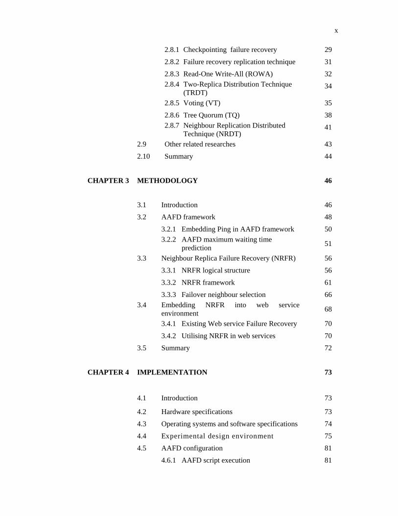
CHAPTER 3 METHODOLOGY 46
3.1 Introduction 46
3.2 AAFD framework 48
3.2.1 Embedding Ping in AAFD framework 50
3.2.2 AAFD maximum waiting time prediction 51
3.3 Neighbour Replica Failure Recovery (NRFR) 56
3.3.1 NRFR logical structure 56
3.3.2 NRFR framework 61
3.3.3 Failover neighbour selection 66
3.4 Embedding NRFR into web service environment 68
3.4.1 Existing Web service Failure Recovery 70
3.4.2 Utilising NRFR in web services 70
3.5 Summary 72
CHAPTER 4 IMPLEMENTATION 73
4.1 Introduction 73
4.2 Hardware specifications 73
4.3 Operating systems and software specifications 74
4.4 Experimental design environment 75
4.5 AAFD configuration 81
4.6.1 AAFD script execution 81

xi
4.6 NRFR configuration 83
4.7 AAFD and NRFR execution 86
4.8 Experimental test scenarios 89
4.9 Summary 96
CHAPTER 5 RESULTS AND ANALYSIS 97
5.1 Introduction 97
5.2 Failure detection results analysis 97
5.2.1 Fail-stop failure detection results analysis 108
5.3 Failure recovery results analysis 111
5.4 Inter-dependent distributed system availability 116 prediction model
5.4.1 TRDT availability prediction model 117
5.4.2 NRDT availability prediction Model 119
5.4.3 TRDT and NDRT availability prediction comparison 122
5.5 Summary 125
CHAPTER 6 CONCLUSION AND FUTURE WORKS 126
6.1 Conclusion 126
6.2 Future Works 129
REFERENCES 131
APPENDIX 138

xii
LIST OF TABLES
3.1 An example of sampling list S 52 3.2 The registered nodes status 58 3.3 Primary data file checksum for each node 59 3.4 Logical neighbour site 59 3.5 Node weighted information 60 3.6 The checksum data file of all nodes in content index table 60
4.1 Hardware specifications 74
4.2 Operating Systems and system development tools 74
specification
4.3 The local IP address and datafiles for each member site 80
5.1 AAFD and other failure detection techniques 100
5.2 Summary of the performance results for site2 106
5.3 Comparison of performance detection between AAFD and other
techniques
107
5.4 Fail-stop failure comparison between GHM, Elhadef and AAFD 111
5.5 The comparison of the size of replicas for a data item under different
set of n sites for various replication techniques
113
5.6 The comparison of fail-stop failure occurrences by number of replica 113
5.7 The recovery time comparison for the five protocols under 114
different set of n sites
5.8 The components availabilities of an interdependent distributed 116
system
5.9 TRDT high availability for various servers 119
5.10 NRDT high availability for various servers 122
5.11 The availabilities predictions comparison between NRDT 123
and TRDT
5.12 TRDT availability prediction over an extended period of 10 123
years
5.13 NRDT availability prediction over an extended period of 10 124
years

xiii 5.14 The availability prediction comparison for NRDT and TRDT 124
over an extended period of 10 year

xiv
LIST OF FIGURES
2.1 Availability in series 12
2.2 Availability in parallel 12
2.3 Availability in joint parallel with series 13
2.4 The Heartbeat model for object monitoring 19
2.5 The Pull model for object monitoring 20
2.6 The architecture of the GHM failure detection 21
2.7 The values of S as a histogram 26
2.8 The probability of cumulative frequencies of the values in S 27
2.9 Data replica distribution technique when N = 2n 34
2.10 Application architecture of TRDT 35
2.11 A tree organization of 13 copies of a data object 38
2.12 An example of a write quorum required in TQ technique 39
2.13 Node with master/primary data file 41
2.14 Examples of data replication in NRDT 42
2.15 A NRDT with 5 nodes 42
3.1 Communication model for the proposed failure detection
methodology
47
3.2 Affirmative adaptive failure detection (AAFD) framework 49
3.3 The AAFD timeline diagram 51
3.4 AAFD algorithm 54
3.5 NRFR logical structure for recovery 57
3.6 The NRFR Framework 63
xv 3.7 Trace and validate neighbour nodes 64
3.8 A failover neighbour activates the virtual IP and starts the
effected services
66
3.9 NRFR algorithm 65
3.10 Web service architectural model for applying NRFR 69
3.11 Utilising NRFR for auto recovering in web services 71
4.1 High level conceptual design for experimental
implementation
76
4.2 Physical design of the experimental environment 77
4.3 VMware virtualisation environment with resources 78
4.4 VMware screenshot for Site3 terminal 79
4.5 The configuration of local IP address for each sites member 80
4.6 The users list in HBM assigned to all registered sites user 81
4.7 Setup auto run on boot for HB generator daemon 82
4.8 HBM auto detection script at HBM server 82
4.9 Command to start, stop, or restart hb_gen 83
4.10 The AAFD and NRFR implementation diagram 86
4.11 Experimental test scenarios diagram 89
4.12 Site3 starts hb_gen service 90
4.13 Screen shot for running HBM.sh script at HBM server 91
4.14 hb.dat file 91
4.15 Site3 restart the hb_gen service 92
4.16 HBM detects Site3 exceed maximum amount of time but still alive
93
4.17 Site3 run service network stop 94
4.18 HBM detects fail-stop failure on Site3 94
4.19 Fail-stop failure recovery procedure on IS 95
4.20 Site2 with two IP numbers 96
5.1 Frequency of Heartbeat inter-arrival times for Site1 in Histogram 98
5.2 Frequency of Heartbeat inter-arrival times for Site2 in
Histogram
98
5.3 Heartbeat inter-arrival times for Satzger et al.(2008) 99
5.4 Example of inter-arrival time on site2 for 100 HB in sequence
manner
101
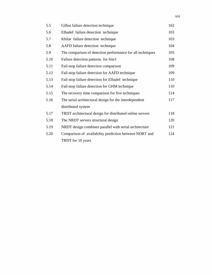
xvi 5.5 Gillen failure detection technique 102
5.6 Elhadef failure detection technique 103
5.7 Khilar failure detection technique 103
5.8 AAFD failure detection technique 104
5.9 The comparison of detection performance for all techniques 105
5.10 Failure detection patterns for Site1 108
5.11 Fail-stop failure detection comparison 109
5.12 Fail-stop failure detection for AAFD technique 109
5.13 Fail-stop failure detection for Elhadef technique 110
5.14 Fail-stop failure detection for GHM technique 110
5.15 The recovery time comparison for five techniques 114
5.16 The serial architectural design for the interdependent
distributed system
117
5.17 TRDT architectural design for distributed online servers 118
5.18 The NRDT servers structural design 120
5.19 NRDT design combines parallel with serial architecture 121
5.20 Comparison of availability prediction between NDRT and
TRDT for 10 years
124

xvii
LIST OF SYMBOLS AND ABBREVIATIONS
AAFD - Affirmative Adaptive Failure Detection
CH - Cluster Head
CPU - Centre Processing Unit
DC - Data Collector
FTP - File Transfer Protocol
GHM - Globus Heartbeat Monitor
HB - Heartbeat
HBM - Heartbeat Monitor
IS - Index Server
MTBF - Mean Time Between Failures
MTTF - Mean Time To Failure
MTTR - Mean Time To Repair
NRDT - Neighbour Replication Distributed Technique
OS - Operating Systems
ROWA - Read-One Write-All
SLAs - Service Level Agreements
SPOF - Single Point Of Failure
SSH - Secure shell protocol
TRDT - Two-Replica Distributed Technique
TQ - Tree Quorum
VT - Voting

xviii
LIST OF APPENDICES
APPENDIX TITLE
PAGE
A Heartbeat node2 (192.168.0.12) 138
B HBM.sh script (failure detection Script) 142
C RecoverPerform.sh script (Recovery Script) 147
D HMax prediction time 154
E VITA 157

CHAPTER 1
INTRODUCTION
In this chapter, the background of the research is outlined, followed by
problem statements, objectives, contributions, scope of the research and lastly, the
organization of the thesis.
1.1 Research background Availability is one of the most important issues in distributed systems (Renesse &
Guerraoui, 2010; Deris et al., 2008; Bora, 2006). With greater numbers of computers
working together, the possibility that a single computer failure can significantly
disrupt the system is decreased (Dabrowski, 2009). One of the benefits of a distributed
system is the increase of parallelism for replication (Renesse & Guerraoui, 2010).
Replication is a fundamental technique to achieve high availability in distributed and
dynamic environments by masking errors in the replicated component (Noor &
Deris, 2010; Bora, 2006). Thus, replication is very important in providing high
availability and efficient distributed system. Distributed systems can therefore lend
themselves in providing high availability (Mamat et al., 2006).
A fail-stop system is one that does not produce any data once it has failed. It
immediately stops sending any events or messages and does not respond to any
messages(Arshad,2006). This type of failures is common in today’s large computing
systems. When a fail-stop failure occurs, a prompt and accurate failure detection with
minimum time to recover are critical factors in providing high availability in
distributed systems. If these factors can efficiently and effectively be handled by a

2
failure detection and recovery technique, it can provide a theoretical and practical
high availability solution for a distributed system.
Since current distributed computing such as grid computing and cloud
computing become larger, increasingly dynamic and heterogeneous. These
distributed systems become more and more complicated. Failures or errors are
arising due to the inherently unreliable nature of the distributed environment include
hardware failures, software errors and other sources of failures. Many failure
detection and recovery techniques have been adopted to improve the distributed
system availability. In addition to the outstanding replication technique for high
availability, failure detection and recovery is an important design consideration for
providing high availability in distributed systems (Dabrowski, 2009; Stelling et al.,
1998; Abawajy, 2004b; Flavio, 2006).
Therefore, failure detection and recovery in distributed computing has
become an active research area (Dimitrova & Finkbeiner, 2009; Siva & Babu 2010;
Khan, Qureshi & Nazir, 2010; Montes, Sánchez & Pérez, 2010; Costan et al., 2010).
Research in failure detection and recovery distributed computing aims at making
distributed systems high availability by handling faults in complex computing
environments. In order to achieve high availability, an autonomous failure detection
and recovery service need to be adopted. An autonomous failure detection and
recovery service is able to detect errors and recover the system without the
participation of any external agents, such as human. It can be restored, or has the
ability of self-healing, then back to the correct state again (Arshad, 2006). If no
failure detection and recovery is provided, the system cannot survive to continue
when one or several processes fail, and the whole program crashes.
Failure detection (or fault detection) is the first essential phase for developing
any fault tolerance mechanism or failure recovery (Avizienis et al., 2004). Failure
detections provide information on faults of the components of these systems (Stalin
et al., 1998).
Failure recovery is the second phase in developing any recovery mechanism
(Avizienis et al., 2004). Replication is one of the core techniques that can be utilised
for failure recovery in distributed and dynamic environments (Bora, 2006).
Exploitation of component redundancy is the basis for recovery in distributed
systems. A distributed system is a set of cooperating objects, where an object could
be a virtual node, a process, a variable, an object as in object-oriented programming,
3
or even an agent in multi-agent systems. When an object is replicated, the application
has several identical copies of the object also known as replicas (Helal, Heddaya &
Bhargava , 1996; Deris et al., 2008). When a failure occurs on a replica, the failure is
masked by its other replicas, therefore availability is ensured in spite of the failure.
Replication mechanisms have been successfully applied in distributed applications.
However, the type of replication mechanisms to be used in the application is decided
by the programmer before the application starts. As a result, it can only be applied
statically. Thus, the development of autonomous failure detection and recovery
model with suitable replication technique and architectural design strategy is very
significant in building high availability distributed systems. 1.2 Problem statements
A study has found fault-detection latencies covered from 55% to 80% of non-
functional periods (Dabrowski et al., 2003). This depends on system architecture and
assumptions about fault characteristics of components. These non-functional periods
happened when a system is uninformed of a failure (or failure detection latency) and
periods when a system attempts to recover from a failure (failure-recovery latency)
(Mills et al., 2004). Even though the development of fault detection mechanism in
large scale distributed system is subject to active research, it still suffers from some
weaknesses (Dabrowski, 2009; Pasin, Fontaine & Bouchenak, 2008; Flavio, 2006).
i) Failure detection trade-offs between accuracy and completeness. Current
failure detection approaches suffer from the weaknesses of either fast detection
with low accuracy or completeness in detecting failures with a lengthy timeout.
Inaccurate detection may result in the recovery malfunction while delays in
detecting a failure will subsequently delay the recovery action. These trade-offs
need to be improved.
ii) Choosing the right replication architectural design strategies are very crucial in
providing high availability and efficient distributed system. This is because
keeping all of the replicas requires extra communication as well as processing
and may delay the recovery process. This will cause the system to be down for
a considerable period of time. In contrast, insufficient replicas can jeopardise
the availability of the distributed system.

4
iii) Although the idea and theory of replication is convincing and robust, practical
implementation of replication technique is difficult to be modelled in real
distributed environment (Christensen, 2006). This is due to the complexity in
the implementation of replication and check pointing techniques. Therefore
they have been studied more theoretically through the use of simulation
technique (Khan, Qureshi & Nazir, 2010). Thus, most of them only discussed
the simulation of the theories rather than its implementation.
iv) Many existing failure recovery techniques have a considerable period of
downtime associated with them. This downtime can cause a significant
business impact in terms of opportunity loss, administrative loss and loss of
ongoing business. There is a need not just to reduce the downtime in the failure
recovery process but also to automate it to a significant degree in order to avoid
errors that are caused by manual failure recovery techniques. 1.3 Objectives The main objectives of this dissertation can be summarized as follows:
i) To propose new approaches for failure detection and an autonomous failure
recovery in distributed system by introducing;
• A new framework for continuous failure detection,
• A new framework for automated failure recovery
ii) To implement failure detection and autonomous failure recovery based on
the proposed approach.
iii) To compare and analyse the performance of the proposed method with
existing approaches.
1.4 Scope The focus of this research is to continuously monitor the failure detection and to
automate the failure recovery in an unpredictable network within Neighbour Replica
Distributed environment with the assumption that failure model is fail-stop failure.

5
1.5 Contributions There are four major contributions in this thesis;
i) Introduced new continuous failure detection approach. The approaches have
improved the detection accuracy and completeness as well as reducing
detection time.
ii) Proposed an autonomous failure recovery approach in a neighbour replica
distributed system that can reduce computation time for failure recovery. The
failure recovery approach also has the capability to determine and select the
neighbour with the best optimal resources which can optimise the system
availability.
iii) The implementation of continuous failure detection and autonomous failure
recovery frameworks using Linux Shell script and tools in the neighbour
replica distributed system. The implementation results showed that
affirmative adaptive failure detection (AAFD) is able to achieve a complete
and accurate detection with prompt timing while neighbour replica failure
recovery NRFR can minimise the recovery time. Hence, by reducing failure
detection latency and recovery processing time, the proposed approaches are
able to reduce the Mean Time To Repair (MTTR) significantly as well as
maximise the system availability or Mean Time Between Failure (MTBF). In
addition, the implementation demonstrated that the proposed failure detection
and recovery is theoretically sound as well as practically feasible in providing
high availability distributed system.
iv) Modelled a realistic and practical logical structure for high availability in
complex and interdependent distributed environment. This model provided
availability predictions for neighbour replica distribution technique (NRDT)
and two replica distribution technique (TRDT).
1.6 Thesis organisation. The work presented in this dissertation is organized into six chapters. The rest of this
document is organized as follows. Chapter two describes preliminary concepts and
related works that are selected from related research. Chapter three proposed a
6
methodology for failure detection and failure recover in neighbour replica distributed
architecture. This chapter discusses in detail the proposed methodology. The
implementation of proposed failure detection and recovery is presented in Chapter
four. Chapter five presents the results and analysis of the proposed approach
implementation and provide in-depth discussion of the implementation results.
Lastly, Chapter six describes the conclusions and possible future work in relation to
this dissertation.

7
CHAPTER 2
LITERATURE REVIEW
This chapter describes related background knowledge and reviews existing literature
on failure detection and recovery. The background knowledge would provide the
information on failure detection metrics, the behaviour of failed systems and
interaction policies. Furthermore, this chapter also discusses and reviews existing
related researches on failure recovery in distributed system which includes, check-
pointing and replication techniques. Since one of the objectives of this thesis is to
automate failure recovery, this chapter will provide detailed review of replication
techniques that best suited the high availability distributed system with self recovery
characteristics. This includes the costs of resources and communication for
replication as well as architectural complexity which will affect the recovery time. It
also highlights the advantages and disadvantages of recent work that have been done
in these fields.
2.1 Introduction Schmidt (2006) defined availability as the frequency or duration in which a service
or a system component is available for use. If this component is needed to provide
the service, outage of a component is also applicable for service availability. In
addition, any features that could help the system to stay operational despite the
occurrences of failures will also be considered as availability.

8
The base availability measurement is the ratio of uptime to total elapsed time
(Schmidt, 2006):
2.2 Availability and unavailability In availability engineering and availability studies, unavailability values are
generally used as compared to the availability values. According to ITEM Software
Inc. (2007), unavailability or Q(t), is the probability that the component or system is
not operating at time t, given that is was operating at time zero. Conversely,
availability, A(t), represents the probability that the component or system is operating
at time t, given that it was operating at time zero. Both Q(t) and A(t) has a numerical
values from 0 to 1 and has no units (ITEM Software Inc, 2007). The unavailability,
Q(t) can also be defined as the component or system probability is in the non-
functional state at time t and is equal to the number of the non-functional
components at time t divided by the total sample. Since a component or system must
be either in the operating or non-operating state at any time, the following
relationship holds true:
A(t) + Q(t) = 1 or Unavailability Q(t) = 1 – A(t) (2.2)
In this relation, the probability of availability with the absent of unavailability
can be calculated. Both parameters can be used in availability assessments, safety
and cost related studies.
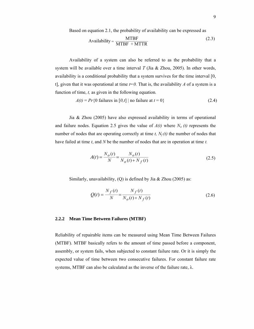
2.2.1 Probability of availability The goal of failure detection and failure recovery study is to reduce the sudden
unavailability so that computer systems can improve availability.
Operational
Availability = --------------------------------------
Operational + Non- Operational
(2.1)
9
Based on equation 2.1, the probability of availability can be expressed as
MTTR+ MTBFMTBFty Availabili = (2.3)
Availability of a system can also be referred to as the probability that a
system will be available over a time interval T (Jia & Zhou, 2005). In other words,
availability is a conditional probability that a system survives for the time interval [0,
t], given that it was operational at time t=0. That is, the availability A of a system is a
function of time, t, as given in the following equation.
A(t) = Pr{0 failures in [0,t] | no failure at t = 0} (2.4)
Jia & Zhou (2005) have also expressed availability in terms of operational
and failure nodes. Equation 2.5 gives the value of A(t) where No (t) represents the
number of nodes that are operating correctly at time t, Nf (t) the number of nodes that
have failed at time t, and N be the number of nodes that are in operation at time t.
)()()()(
)(tNtN
tNN
tNfo
ootA+
== (2.5)
Similarly, unavailability, (Q) is defined by Jia & Zhou (2005) as:
)()()()(
)(tNtN
tNN
tN
fo
fftQ+
== (2.6)
2.2.2 Mean Time Between Failures (MTBF) Reliability of repairable items can be measured using Mean Time Between Failures
(MTBF). MTBF basically refers to the amount of time passed before a component,
assembly, or system fails, when subjected to constant failure rate. Or it is simply the
expected value of time between two consecutive failures. For constant failure rate
systems, MTBF can also be calculated as the inverse of the failure rate, λ.
10
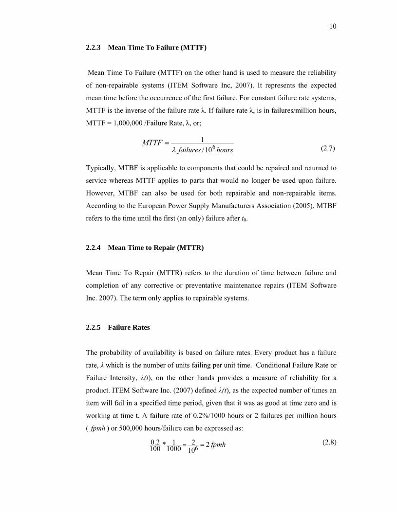
2.2.3 Mean Time To Failure (MTTF) Mean Time To Failure (MTTF) on the other hand is used to measure the reliability
of non-repairable systems (ITEM Software Inc, 2007). It represents the expected
mean time before the occurrence of the first failure. For constant failure rate systems,
MTTF is the inverse of the failure rate λ. If failure rate λ, is in failures/million hours,
MTTF = 1,000,000 /Failure Rate, λ, or;
hoursfailuresMTTF 610/
1λ
=
(2.7)
Typically, MTBF is applicable to components that could be repaired and returned to
service whereas MTTF applies to parts that would no longer be used upon failure.
However, MTBF can also be used for both repairable and non-repairable items.
According to the European Power Supply Manufacturers Association (2005), MTBF
refers to the time until the first (an only) failure after t0.
2.2.4 Mean Time to Repair (MTTR) Mean Time To Repair (MTTR) refers to the duration of time between failure and
completion of any corrective or preventative maintenance repairs (ITEM Software
Inc. 2007). The term only applies to repairable systems.
2.2.5 Failure Rates The probability of availability is based on failure rates. Every product has a failure
rate, λ which is the number of units failing per unit time. Conditional Failure Rate or
Failure Intensity, λ(t), on the other hands provides a measure of reliability for a
product. ITEM Software Inc. (2007) defined λ(t), as the expected number of times an
item will fail in a specified time period, given that it was as good at time zero and is
working at time t. A failure rate of 0.2%/1000 hours or 2 failures per million hours
( fpmh ) or 500,000 hours/failure can be expressed as:
fpmh210
21000
1*1002.0
6 == (2.8)
11
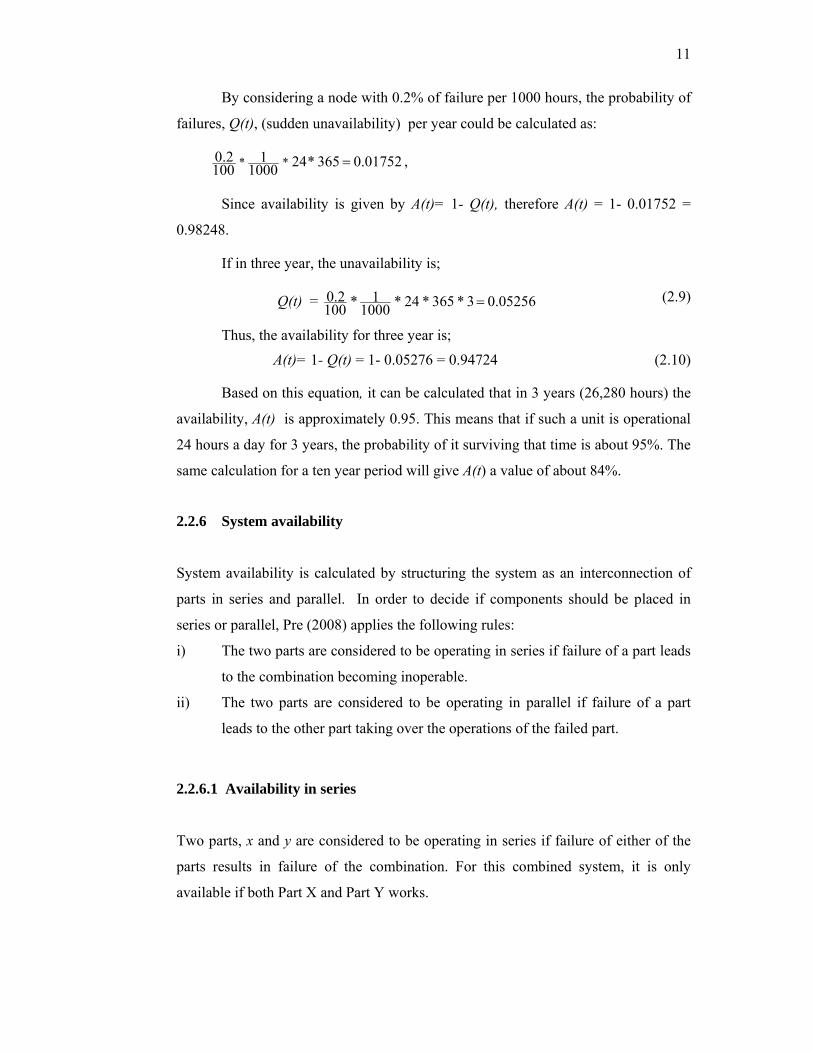
By considering a node with 0.2% of failure per 1000 hours, the probability of
failures, Q(t), (sudden unavailability) per year could be calculated as:
0.01752365*2410001
1002.0 ** = ,
Since availability is given by A(t)= 1- Q(t), therefore A(t) = 1- 0.01752 =
0.98248.
If in three year, the unavailability is;
Q(t) = 0.052563*365*24*10001*100
2.0 = (2.9)
Thus, the availability for three year is; A(t)= 1- Q(t) = 1- 0.05276 = 0.94724 (2.10)
Based on this equation, it can be calculated that in 3 years (26,280 hours) the
availability, A(t) is approximately 0.95. This means that if such a unit is operational
24 hours a day for 3 years, the probability of it surviving that time is about 95%. The
same calculation for a ten year period will give A(t) a value of about 84%.
2.2.6 System availability System availability is calculated by structuring the system as an interconnection of
parts in series and parallel. In order to decide if components should be placed in
series or parallel, Pre (2008) applies the following rules:
i) The two parts are considered to be operating in series if failure of a part leads
to the combination becoming inoperable.
ii) The two parts are considered to be operating in parallel if failure of a part
leads to the other part taking over the operations of the failed part.
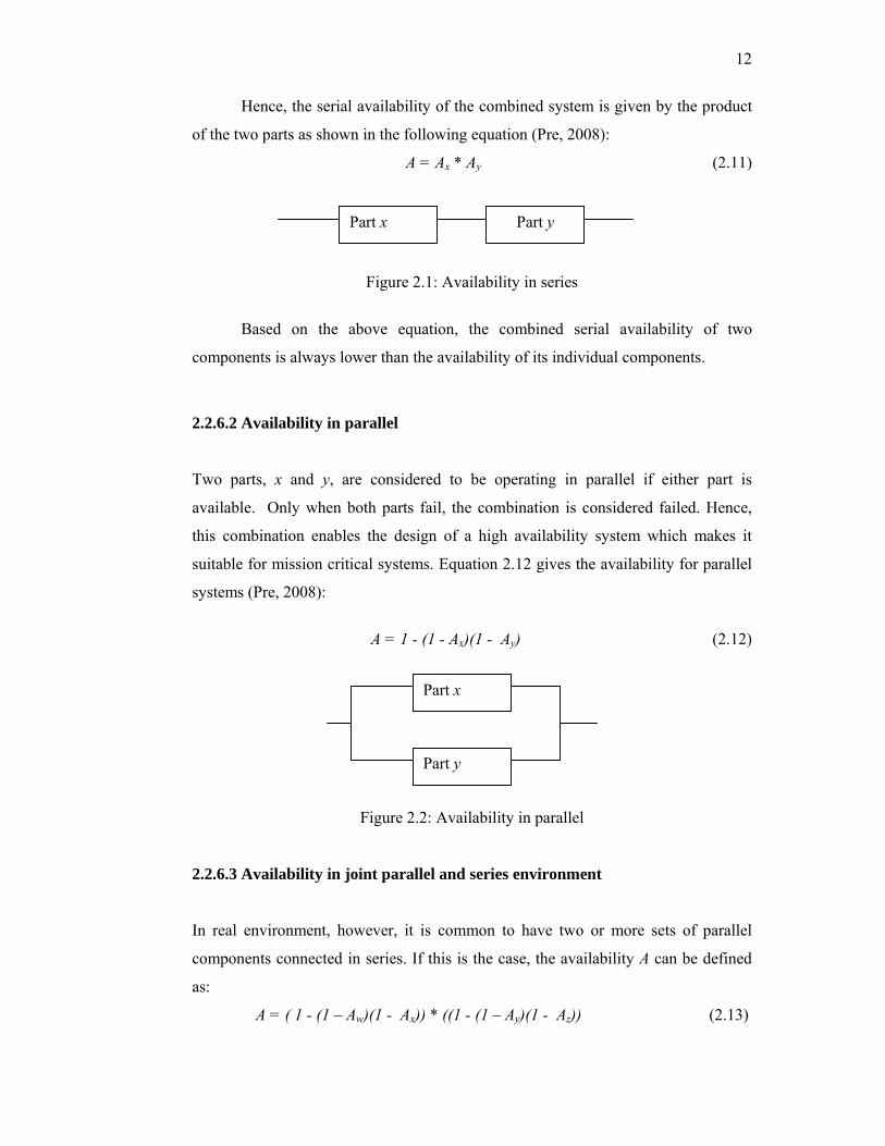
2.2.6.1 Availability in series Two parts, x and y are considered to be operating in series if failure of either of the
parts results in failure of the combination. For this combined system, it is only
available if both Part X and Part Y works.
12
Hence, the serial availability of the combined system is given by the product
of the two parts as shown in the following equation (Pre, 2008):
A = Ax * Ay (2.11)
Figure 2.1: Availability in series
Based on the above equation, the combined serial availability of two
components is always lower than the availability of its individual components.
2.2.6.2 Availability in parallel Two parts, x and y, are considered to be operating in parallel if either part is
available. Only when both parts fail, the combination is considered failed. Hence,
this combination enables the design of a high availability system which makes it
suitable for mission critical systems. Equation 2.12 gives the availability for parallel
systems (Pre, 2008):
A = 1 - (1 - Ax)(1 - Ay) (2.12)
Figure 2.2: Availability in parallel 2.2.6.3 Availability in joint parallel and series environment In real environment, however, it is common to have two or more sets of parallel
components connected in series. If this is the case, the availability A can be defined
as:
A = ( 1 - (1 – Aw)(1 - Ax)) * ((1 - (1 – Ay)(1 - Az)) (2.13)
Part x
Part y
Part x Part y

13
Figure 2.3: Availability in joint parallel with series 2.2.7 Availability in distributed system Data availability in parallel distributed systems could be improved by storing
multiple copies of data at different sites. With this redundancy, data could be made
available to users despite site and communication failures. In the parallel distributed
system, the system works unless all nodes fail. Connecting machines in parallel
contribute to the system redundancy reliability enhancement.
Let A = availability, Q = unavailability, then the system unavailability as
given by Koren and Krihna (2007) is as follow:
Q = Q1 * Q2 * Q3 *...* Qn
Q = (1 – A1) * (1 – A2) * (1 – A3) * (1 – An)
(2.14)
Thus, the availability of the distributed parallel system can be calculated as:
AS = 1- QS =1- (Q1* Q2 * Q3 *...* Qn)
= 1- [(1 – A1) * (1 – A2) * ..* (1 – An)]
= ∏=
−−n
iiA
1)1(1
(2.15)
To illustrate this, let us take a system that consists of three nodes connected in
parallel. The availability of these nodes are 0.9, 0.95 and 0.98 respectively. The
overall system availability is given by:
A = 1-(1-0.9)*(1-0.95)*(1-0.98) = 1-0.1*0.05*0.02 = 1-0.0001
A = 0.99990
(2.16)
Part w
Part x
Part y
Part z
14
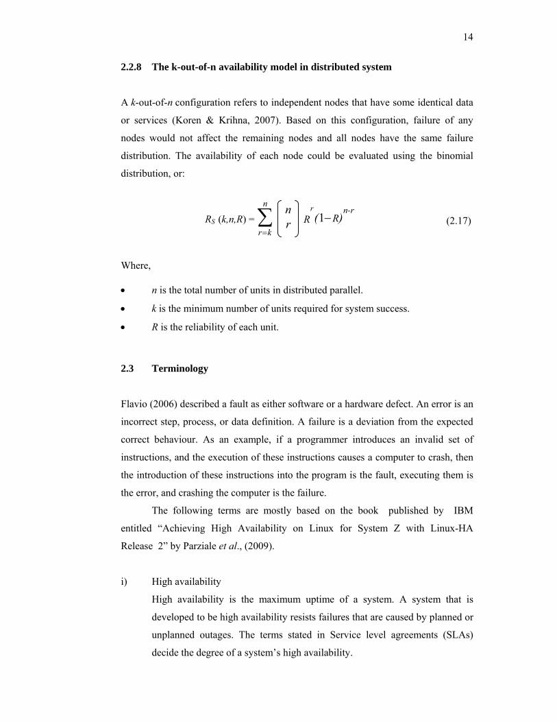
2.2.8 The k-out-of-n availability model in distributed system A k-out-of-n configuration refers to independent nodes that have some identical data
or services (Koren & Krihna, 2007). Based on this configuration, failure of any
nodes would not affect the remaining nodes and all nodes have the same failure
distribution. The availability of each node could be evaluated using the binomial
distribution, or:
(2.17)
Where,
• n is the total number of units in distributed parallel.
• k is the minimum number of units required for system success.
• R is the reliability of each unit.
2.3 Terminology Flavio (2006) described a fault as either software or a hardware defect. An error is an
incorrect step, process, or data definition. A failure is a deviation from the expected
correct behaviour. As an example, if a programmer introduces an invalid set of
instructions, and the execution of these instructions causes a computer to crash, then
the introduction of these instructions into the program is the fault, executing them is
the error, and crashing the computer is the failure.
The following terms are mostly based on the book published by IBM
entitled “Achieving High Availability on Linux for System Z with Linux-HA
Release 2” by Parziale et al., (2009).
i) High availability
High availability is the maximum uptime of a system. A system that is
developed to be high availability resists failures that are caused by planned or
unplanned outages. The terms stated in Service level agreements (SLAs)
decide the degree of a system’s high availability.
∑=
n
kr
n r
1n-r
)( RRr
−RS (k,n,R) =

15
ii) Continuous operation
Continuous operation is an uninterrupted or non-disruptive level of operation
where changes to hardware and software are apparent to users. Planned
outages normally take place in environments that are designed to provide
continuous operation. These kinds of environments are designed to avoid
unplanned outages.
iii) Continuous availability
Continuous availability is an uninterrupted, non-disruptive, level of service
that is provided to users. It provides the highest level of availability that can
possibly be achieved. Planned or unplanned outages of hardware or software
cannot exist in environments that are designed to provide continuous
availability.
iv) Failover
Failover is the procedure in which one or more node resources are transferred
to another nodes or nodes in the same cluster because of failure or
maintenance.
v) Failback
Failback is the procedure in which one or more resources of a non-functional
node are returned to its original owner once it becomes available.
vi) Primary (active) node
A principal or main node is a member of a cluster, which holds the cluster
resources and runs processes against those resources. When the node is
conciliated, the ownership of these resources stops and is passed to the
standby node.
vii) Standby (secondary, passive, or failover) node
A standby node, also known as a passive, secondary or failover node is a
member of a distributed system that is able to access resources and running
processes. However, it is in a standby position until the principal node is
conciliated or has to be stopped. At that point, all resources fail over to the
standby node, which becomes the active node.
viii) Single point of failure
A single point of failure (SPOF) exists when a hardware or software
component of a system can potentially bring down the entire system without
16
any means of quick recovery. High availability systems tend to avoid a single
point of failure by using redundancy in every operation.
ix) Cluster
A cluster is a group of nodes and resources that act as one entity to enable
high availability or load balancing capabilities.
x) Outage
For the intention of this thesis, outage is the failure of services or applications
for a particular period of time. An outage can be planned or unplanned:
• Planned outage
Planned outage takes place when services or applications are
interrupted because of planned maintenance or changes, which are
expected to be reinstated at a specific time.
• Unplanned outage
Unplanned outage takes place when services or applications are
interrupted because of events that are out of control such as natural
disasters. Unplanned outages can also be caused by human errors and
hardware or software failures.
xi) Uptime
Uptime is the duration of time when applications or services are available.
xii) Downtime
Downtime is the duration of time when services or applications are not
available. It is usually calculated from the time that the outage takes place to
the time when the services or applications are available.
xiii) Service level agreement
Service Level Agreements (SLAs) ascertain the degree of responsibility to
maintain services that are available to users, costs, resources, and the
complexity of the services. For example, a banking application that handles
stock trading must maintain the highest degree of availability during active
stock trading hours. If the application goes down, users are directly affected
and, as a result, the business suffers. The degree of responsibility varies
depending on the needs of the user.

17
2.4 Failure detection Failure detection is a process in which information about faulty nodes is collected
(Siva & Babu, 2010). This process involves isolation and identification of a fault to
enable proper recovery actions to be initiated. It is an important part of failure
recovery in distributed systems.
Chandra & Toueg (1996) characterize failure detectors by specifying their
completeness and accuracy properties (Elhadef & Boukerche, 2007). The
completeness of a failure detector refers to its capability of suspecting every faulty
node permanently. While, the accuracy refers to its capability of not suspecting fault-
free ones.
Stelling et al. (1999) considered the main concerns or requirements that
should be addressed in designing a fault detector for grid environments. These
include:
i) Accuracy and completeness. The fault detector must identify faults
accurately, with both false positives and false negatives being rare.
ii) Timeliness. Problems must be identified in a timely manner in order for
responses and corrective actions to be initiated as soon as possible.
Chen et al. (2000) analysed the quality of service (QoS) of failure detectors
and proposed that the measurement of QoS should adhere to the following metrics:
i) Detection time (TD): TD is the time that passes from q’s crash to the time
when q starts to suspect p permanently.
ii) Mistake recurrence time (TMR): The mistake recurrence is the time between
false detections.
In order to formally classify the QoS metrics, Chen et al. (2000) identified
state transitions of a failure detector as “when a failure detector monitors a monitored
process, at any time, the failure detector’s state either trusts or suspects the monitored
process’s liveness. If a failure detector transfers from a trust state to a suspect state,
then an S-transition occurs, if a failure detector transfers from a Suspect state to a
Trust state then a T-transition occurs”. Ma (2007) recommended a set of QoS metrics
to measure the completeness, accuracy and speed of unreliable failure detectors. QoS
in this context means measures that indicate (1) how fast a failure detector detects
actual failures, and (2) how well it avoids false detections.

18
2.5 Behaviour of failed systems In distributed systems, failures do occur. The types of failures can cause the system
to behave in a certain way. While there are slight discrepancies in literature regarding
their definitions (Satzger et al., 2008), Arshad (2006) classifies possible behaviour of
systems following a failure into three types which are:
i) A crash-recovery failure model is a fail-stop failure in which once it has
failed, it would not be able to output any action or trigger any events.
ii) A byzantine system is one that does not stop after a failure but instead
behaves in an inconsistent way. It may send out wrong information, or
respond late to a message.
iii) A fail-fast system is one that behaves like a Byzantine system for some time
but moves into a fail-stop mode after a short period of time.
This thesis focuses on distributed system components or nodes that have fail-
stop behaviour. It does not matter what type of faults or failures that have caused this
behaviour but it is necessary that the system does not perform any operation once it
has failed. In other words it just stops doing anything following a failure.
2.6 Interaction policies The failure detectors and the monitored components commonly communicate
through either two interaction protocols. One is the heartbeat model and the other is
the pull or ping model. These behaviours of monitoring protocols are used by failure
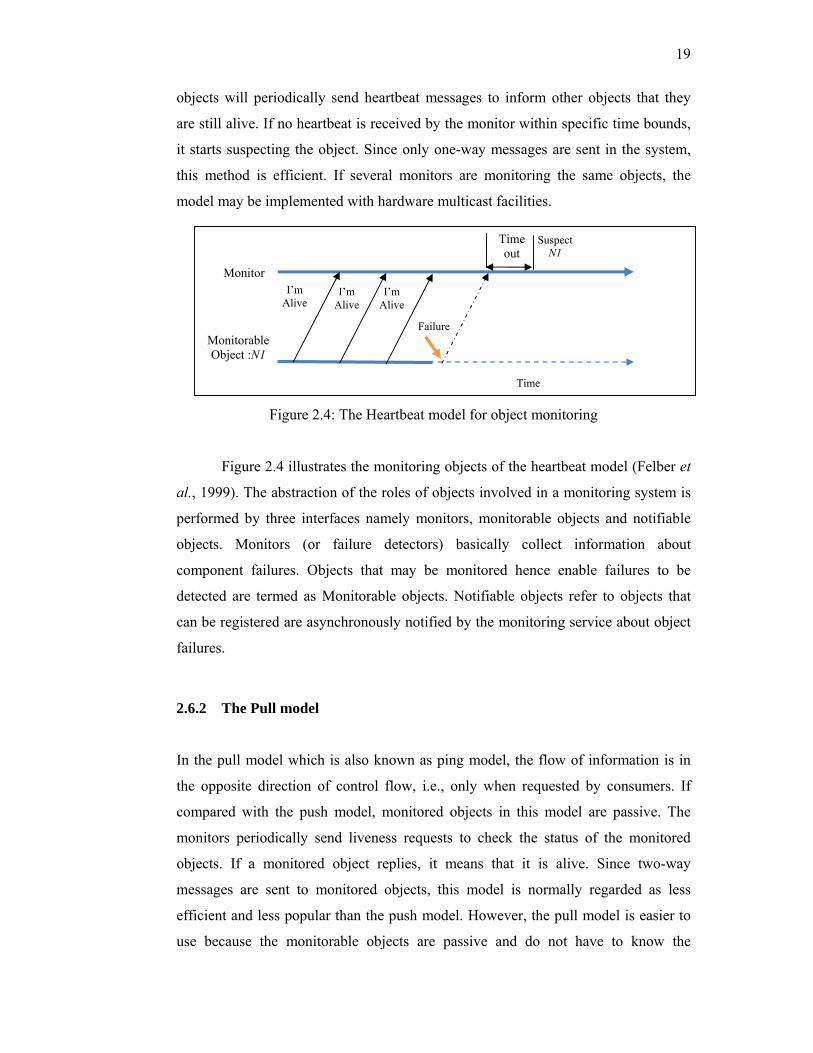
detector to monitor system components (Felber et al., 1999).
2.6.1 The Heartbeat model The heartbeat model or push model is the most common technique for monitoring
crash failure (Mou, 2009). Many state-of-the-art failure detector approaches were
based on heartbeats (Hayashibara & Takizawa 2006; Satzger et al., 2007; Satzger et
al., 2008; Dobre et al., 2009; Noor & Deris, 2009).
In the push model, the direction of control flow matches the direction of
information flow. In addition, the model has active monitorable objects. These
19
objects will periodically send heartbeat messages to inform other objects that they
are still alive. If no heartbeat is received by the monitor within specific time bounds,
it starts suspecting the object. Since only one-way messages are sent in the system,
this method is efficient. If several monitors are monitoring the same objects, the
model may be implemented with hardware multicast facilities.
Figure 2.4: The Heartbeat model for object monitoring
Figure 2.4 illustrates the monitoring objects of the heartbeat model (Felber et
al., 1999). The abstraction of the roles of objects involved in a monitoring system is
performed by three interfaces namely monitors, monitorable objects and notifiable
objects. Monitors (or failure detectors) basically collect information about
component failures. Objects that may be monitored hence enable failures to be
detected are termed as Monitorable objects. Notifiable objects refer to objects that
can be registered are asynchronously notified by the monitoring service about object
failures.
2.6.2 The Pull model In the pull model which is also known as ping model, the flow of information is in
the opposite direction of control flow, i.e., only when requested by consumers. If
compared with the push model, monitored objects in this model are passive. The
monitors periodically send liveness requests to check the status of the monitored
objects. If a monitored object replies, it means that it is alive. Since two-way
messages are sent to monitored objects, this model is normally regarded as less
efficient and less popular than the push model. However, the pull model is easier to
use because the monitorable objects are passive and do not have to know the
Time out
Monitor
Time
I’m Alive
Suspect N1
I’m Alive
I’m Alive
FailureMonitorable Object :N1
20
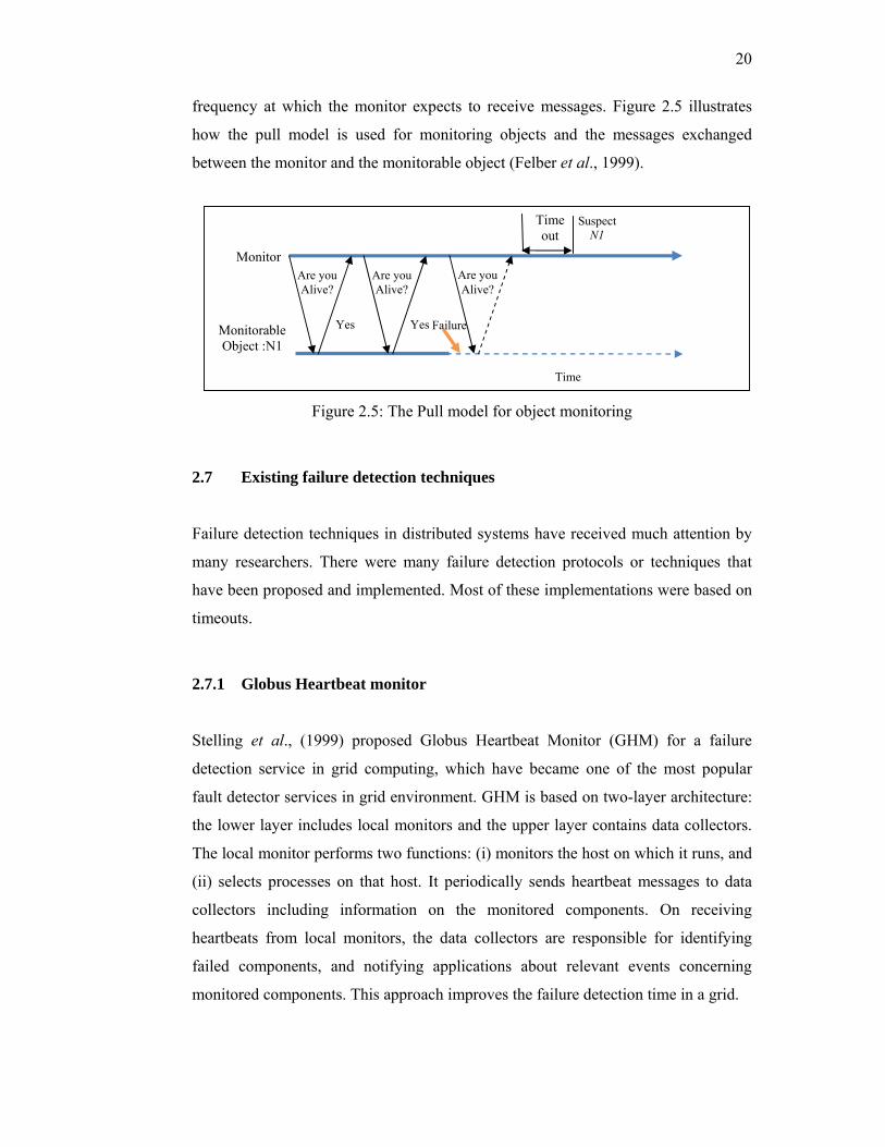
frequency at which the monitor expects to receive messages. Figure 2.5 illustrates
how the pull model is used for monitoring objects and the messages exchanged
between the monitor and the monitorable object (Felber et al., 1999).
Figure 2.5: The Pull model for object monitoring
2.7 Existing failure detection techniques Failure detection techniques in distributed systems have received much attention by
many researchers. There were many failure detection protocols or techniques that
have been proposed and implemented. Most of these implementations were based on
timeouts.
2.7.1 Globus Heartbeat monitor Stelling et al., (1999) proposed Globus Heartbeat Monitor (GHM) for a failure
detection service in grid computing, which have became one of the most popular
fault detector services in grid environment. GHM is based on two-layer architecture:
the lower layer includes local monitors and the upper layer contains data collectors.
The local monitor performs two functions: (i) monitors the host on which it runs, and
(ii) selects processes on that host. It periodically sends heartbeat messages to data
collectors including information on the monitored components. On receiving
heartbeats from local monitors, the data collectors are responsible for identifying
failed components, and notifying applications about relevant events concerning
monitored components. This approach improves the failure detection time in a grid.
Time out
Monitor
Time
Suspect N1
FailureMonitorable Object :N1
Are you Alive?
Yes
Are you Alive?
Yes
Are you Alive?

21
Each local monitor in this approach broadcasts heartbeats to all data
collectors. Globus toolkit has been designed to use existing fabric components,
including vendor-supplied protocols and interfaces (Hayashibara & Takizawa, 2006).
Figure 2.6: The architecture of the GHM failure detection (Stelling et al., 1999)
The architecture of the GHM failure detection service grid shown in Figure
2.6 may change its topology by component leaving/joining at runtime but the
proposed architecture is static and does not adapt well to such changes in a system
topology. Recently, International Business Machines (IBM) (Parziale et al., 2009)
have utilised the Heartbeat Release 2 (released in 2005) in achieving high availability
on Linux for IBM System Z. This heartbeat is able to scale up to 16 nodes. However,
the Heartbeat Release 2 still maintains the fixed interval time and timeout delay as
Heartbeat Release 1. However, few bottlenecks have been identified as put by
Abawajy (2004b) “they scale badly in that the number of members that are being
monitored require developers to implement fault tolerance at the application level”.
Pasin, Fontaine and Bouchen (2008) also found that they are difficult to implement
and have high-overhead.
Failure Detection and Recovery Services (FDS) improves the GHM with
early detection of failures in applications, grid middleware and grid resources
(Abawajy, 2004b). The classical heartbeat approach suffers from two main
weaknesses;
i) The detection time depends on the last heartbeat.
Data Collector
Host l Local Monitor
Minitored Process
Process registration
Process statusinquiry
Data Collector
Host N Local Monitor
Minitored Process
Process registration
Process status inquiry
■■■
22
ii) It relies on a fixed timeout delay that does not take into account the network
and system’s load.
The first weakness may have a negative impact on the accuracy of the failure
detector since premature timeouts may occur. For the second weakness, a node may
be mistakenly suspected as faulty if it slows down due to heavy workload or if the
network suffers from links failure that may delay the delivery of messages.
2.7.2 Scalable failure detection Gillen et al. (2007) have designed an adaptive version of the Node-Failure Detection
NFD subsystem. In this version, the failure-detection thresholds used by individual
Monitors are increasingly adjusted on a per-node basis. A simplistic approach was
used to monitor adaptation. Every time the monitor detected a false positive on that
node, the Monitor’s detection threshold, Th for a node is multiplied by a configurable
value, k. In the implementation, they set the value of threshold to 2 (the same value
of k is used for all nodes.) Th+1 = k(Sn).They concluded that the best way to avoid a
large number of false positives caused by dropped heartbeat packets is to set Th to
be at least twice the heartbeat generation period. This enables the system to avoid
declaring a false failure in the case of disjointed single-packet losses without
incurring the overhead from sending more packets.
2.7.3 Adaptive failure detection Adaptive failure detectors can adapt to change network conditions (Chen, 2002;
Hayashibara et al., 2004). The approaches were based on periodically sent heartbeat
messages. A network can behave significantly different during high traffic times and
low traffic times with respect to probability of message loss, the expected delay for
message arrivals, and the variance of this delay. In order to meet the current
conditions of the system, adaptive failure detectors will arrange their parameters
accordingly. In this case, the parameter is the predicted arrival time of future
heartbeat message. For example, the next heartbeat message will arrive within 2
seconds. Thus, this makes adaptive failure detectors highly desirable. In large scale
networks, adaptive approaches were proved to be more efficient than approaches
23
with constant timeout (Khilar, Singh & Mahapatra, 2008; Gillen et al., 2000; Satzger
et al., 2008).
Chen et al. (2002) have proposed a well-known implementation for a failure
detector that adapts to changes in network conditions. It was based on a probabilistic
analysis of a network traffic called adaptive failure. Adaptive failure detectors are
extended implementations that adapt dynamically to their environment (i.e., network
condition) and to change application behaviour. These adapters are basically
implemented based on the concepts of unreliable failure detectors or the legacy
timeout-based failure detection. A timeout is adjusted according to network condition
and requirement from an application. This technique compute an estimation of the
arrival time of the next heartbeat using arrival times sampled in the recent past. The
timeout is set according to this estimation and a safety margin, and recomputed for
each interval. The safety margin is set by application QoS requirements (e.g., upper
bound on detection time) and network characteristics (e.g., network load). Based on
data failure samples, detectors generate a suspicion value which indicates whether a
node has failed or not. Failure detectors differ in the way the suspicion value is
computed but they all are dependent on the input from the sample base.
Bertier & Marin (2002) have integrated Chen’s estimation with another
estimation developed by Jacobson (1998) for a different context. Their approach is
similar to Chen’s, however they did not use a constant safety margin but computed it
with Jacobson’s approach. Elhadef & Boukerch (2007) proposed a method to
estimate the arrival time of the heartbeat messages where the arrival time of the next
heartbeat of a node is computed by averaging the n last arrival times. In their
implementation, Bertier’s approach is improved and utilised. Process p manages a
list S based on the information it receives about the inter arrival times of the
heartbeats. The equation for heartbeat arrival prediction for this approach is given
as:-
|| 11n S
SS
n
ii∑
==+ (2.18)
where
S = [1.083s, 0.968s, 1.062s, 0.993s, 0.942s, 2.037s, . . .]
Si = {x | x ∈ S and x ≠ ∅}
sn+1 = Inter arrival time of next heartbeat message.
24
Khilar, Singh & Mahapatra (2008) have proposed an adaptive failure
detection service for large scale ad hoc networks using an efficient cluster based
communication architecture. This failure detection service (after this, it is called
Khilar’s approach) adapted the detection parameter to the current load of the wireless
ad hoc network. In this proposed approach, a heartbeat based testing mechanism is
used to detect failure in each cluster and take the advantage of cluster based
architecture to forward the failure report to other cluster and their respective
members. In Khilar’s failure detection approach, each cluster head maintains a
heartbeat table received for each member node. Cluster head, CH also stores the
arrival time of last n heartbeat messages for each member node. Initially, the table
has a fixed timeout period for each node. When a heartbeat from a particular member
is received, a new freshness point is calculated using the arrival time of this heartbeat
and previous heartbeat messages and new timeout period is set to be equal to this
freshness point, Sn+1 = Sn or Hmax = Sn.
2.7.4 Lazy Failure Detection Lazy Failure detection approach (Fetzer et al., 2001) attempt to reduce the
networking overhead that arises e.g. from sending heartbeat messages. To achieve
this, detection processes monitor each other by using application messages whenever
possible to get information on processor failures. This protocol requires each
message to be acknowledged. Only when two processes are not communicating, then
failure detection messages are used (Satzger et al., 2008).
A heartbeat-style failure detector is referred to as lazy if it uses a technique to
reduce the networking overhead caused by sending heartbeat messages. In other
word, this approach only send heartbeat messages if it really have to and is thus
called lazy. In this context, it is important to distinguish between application
messages and heartbeat messages. While the former are sent by the application and
unavoidable, heartbeat messages are sent by failure detectors.
Satzger et al. (2008) proposed a lazy monitoring approach aims at reducing
the network load without the negative effects on the detection time. Quite the
contrary, it allows for a better training of the failure detector as it provides more data
and thus can further improve the quality of the generated suspicion information. This

131
REFERENCES
Abawajy J. (2004a). Fault-tolerant scheduling policy for Grid computing systems.
Proceedings of the 18th International Parallel and Distributed Processing
Symposium, April 2004. Los Alamitos, CA: IEEE Computer Society Press.
pp. 238–244.
Abawajy, J. (2004b). Fault detection service architecture for Grid computing
systems. LNCS, 3044. Berlin, Heidelberg: Springer-Verlag. pp. 107–115.
Agrawal, D. and El Abbadi, A. (1992). The generalized tree quorum protocol: an
efficient approach for managing replicated data. ACM Trans. Database
System. pp. 689-717.
Ahmad, N. (2007). Managing replication and transactions using neighbour
replication on data grid Database design. Ph.D. Thesis. Universiti Malaysia
Terengganu.
Amazon.com Inc. (2010). Amazon Simple Storage Service (Amazon S3). Retrieved
on September 12, 2010 from http://aws.amazon.com/s3
Andrieux, A., Czajkowski, K., Dan, A., Keakey, K., Ludwig, H., Nakata, T., Pruyne,
J., Rofrano, J., Tuecke, S. & Xu, M. (2007). Web services agreement
specification (WS-Agreement). GFD.107, Open Grid Forum.
Andrzejak, A., Graupner, S., Kotov, V. & Trinks, H. (2002). Algorithms for self-
organization and adaptive service placement in dynamic distributed systems.
HPL-2002-259, Hewlett Packard Corporation.
Arshad N. (2006). A Planning-Based Approach to Failure Recovery in Distributed
Systems. Ph.D. Thesis. University of Colorado.
Avizienis, A., Laprie, J., Randell, B., & Landwehr, C. (2004). Basic concepts and
taxonomy of dependable and secure computing. IEEE Transactions on
Dependable and Secure Computing, 1(1), pp. 11–33.
132
Bertier, M. & Marin, P. (2002). Implementation and performance evaluation of an
adaptable failure detector. Proceedings of the Intl. Conf. on Dependable
Systems and Networks. pp. 354 – 363.
Bora S. (2006). A Fault Tolerant System Using Collaborative Agents. LNAI, 3949.
Berlin, Heidelberg: Springer-Verlag. pp. 211– 218.
Boteanu A, Dobre C, Pop F & Cristea, V (2010). Simulator for fault tolerance in
large scale distributed systems. Proceedings of the 2010 IEEE 6th
International Conference on Intelligent Computer Communication and
Processing. pp. 443-450.
Budati K, Sonnek J, Chandra A & Weissman J. (2007). RIDGE: Combining
reliability and performance in open Grid platforms. Proceedings of the 16th
International Symposium on High Performance Distributed Computing
(ISHPDC2007). New York, USA: ACM Press. pp. 55–64.
Chen, W., Toueg, S. & Aguilera, M.K. (2000). On the quality of service of failure
detectors. Proceedings of the International Conference on Dependable
Systems and Networks New York. IEEE Computer Society Press.
Chen, W. Toueg, S. & Aguilera, M.K. (2002). On the QoS of failureDetectors.
IEEE Trans. Computers, 51(5), pp. 561–580.
Chervenak, A., Vellanki, V.& Kurmas, Z. (1998) Protecting file systems: A survey
of backup techniques. In: Proc. of Joint NASA and IEEE Mass Storage
Conference. Los Alamitos: IEEE Computer Society Press.
Christensen N. H. (2006). A formal analysis of recovery in a preservational data
grid. Proceedings of the 23rd IEEE Conference on Mass Storage Systems and
Technologies, College Park, Maryland USA.
Cooper M. (2008). Advanced Bash-Scripting Guide, An in-depth exploration of the
art of shell, Retrieved on October 9, 2008 from http://theriver.com.
Costan, A. Dobre, C. Pop, F. Leordeanu, C. & Cristea, V. ( 2010). A fault tolerance
approach for distributed systems using monitoring based replication.
Proceedings of the 2010 IEEE 6th International Conference on Intelligent
Computer Communication and Processing. pp. 451-458.
Dabrowski, C., Mills, K. & Rukhin, A. (2003). A Performance of Service-Discovery
Architectures in Response to NodeFailures, Proceedings of the 2003
International Conferenceon Software Engineering Research and Practice
(SERP'03): CSREA Press. pp. 95-10.
133
Dabrowski, C. (2009). Reliability in grid computing, Concurrency Computation: Practice
and Experience. Wiley InterScience.
Deris, M.M. (2001). Efficient Access of Replicated Data in Distributed Database
Systems. Ph.D. Thesis, Universiti Putra Malaysia.
Deris, M.M. , Abawajy, J. H. & Mamat, A. (2008). An efficient replicated data
access approach for large-scale distributed systems. Future Generation
Comp. Syst. 24(1), pp. 1-9.
Deris M.M., Ahmad N, Saman M. Y., Ali N. & Yuan Y. (2004). High System
Availability Using Neighbor Replication on Grid. IEICE Transactions 87-D
(7), pp. 1813-1819.
Dimitrova, R. & Finkbeiner, B. (2009). Synthesis of Fault-Tolerant Distributed
Systems LNCS, 5799. Berlin Heidelberg: Springer-Verlag. pp. 321–336.
Elhadef, M & Boukerche, A. (2007). A Gossip-Style Crash Faults Detection Protocol
for Wireless Ad-Hoc and Mesh Networks. Proceedings of Int. Conf. IPCCC.
pp. 600-602.
European Power Supply Manufacturers Association. (2005). Guidelines to
Understanding Reliability Prediction. Wellingborough, Northants, U.K.
Felber, P D´efago, X. Guerraoui, R. & Oser, P. (1999). Failure detectors as first
class objects. Proceedings of the 9th IEEE Int’lSymp. on Distributed Objects
and Applications. pp. 132–141.
Fetzer C. Raynal M. & Tronel F. (2001). An adaptive failure detection protocol.
Proceedings of the 8th IEEE Pacific Rim Symp. on Dependable Computing.
pp. 146 - 153.
Figgins, S. Siever, E. & Weber, A. (2003). Linux in a Nutshell, 4th Edition O'Reilly,
USA.
Flavio, J. (2006). Coping with dependent failures in distributed systems. Ph.D.
Thesis, University of California, San Diego.
Genaud, S. & Rattanapoka, C. (2007). P2P-MPI: A peer-to-peer framework for
robust execution of message passing parallel programs on Grids. Journal of
Grid Computing, 5(1), pp. 27–42.
Gillen, M. Rohloff, K. Manghwani, P. & Schantz, R (2007). Scalable, Adaptive,
Time-Bounded Node Failure Detection. Proceedings of the 10th IEEE High
Assurance Systems Engineering Symposium (HASE '07). DC, USA.
134
Goodale. T, Allen, G., Lanfermann, G., Masso, J., Radke, T., Seidel, E., Shalf, J.
(2003). The cactus framework and toolkit: Design and applications. LNCS,
2565. Berlin Heidelberg: Springer. pp. 15–36.
Hayashibara, N. Defago, X. Yared R.& Katayama T. (2004).The f accrual failure
detector. In 23rd IEEE International Symposium on Reliable Distributed
Systems(SRDS’04): IEEE Computer Society. pp. 66–78.
Hayashibara, N. & Takizawa, M. (2006).Design of a notification system for the φ
accrual failure detector. Proceedings of the 20th International Conference on
Advanced Information Networking and Applications - Volume 1 (AINA'06).
pp. 87-97.
Helal, A., Heddaya, A. & Bhargava, B. (1996). Replication Techniques in
Distributed Systems: Kluwer Academic Publishers.
Hwang, S. & Kesselman, C. (2003). Introduction Requirement for Fault Tolerance in
the Grid, Related Work. A Flexible Framework for Fault Tolerance in the
Grid. Journal of Grid Computing 1, pp. 251-272.
ITEM Software, Inc.(2007) , Reliability Prediction Basics, Hampshire ,U.K.
Jia, W. & Zhou, W. (2005), Distributed Network Systems: From Concepts to
Implementations. Springer Science and Business Media.
Khan, F.G., Qureshi, K. & Nazir, B. (2010). Performance evaluation of fault
tolerance techniques in grid computing system. Computers & Electrical
Engineering Volume 36, Issue 6, Elsevier B.V. pp. 1110-1122.
Khilar, P. Singh, J.& Mahapatra, S. (2008). Design and Evaluation of a Failure
Detection Algorithm for Large Scale Ad Hoc Networks Using Cluster Based
Approach. International Conference on Information Technology 2008, IEEE.
Koren, I. & Krishna C. M. (2007), Fault-Tolerant Systems. San Francisco, CA:
Morgan-Kaufman Publishers.
Parziale, L., Dias, A., Filho, L.T., Smith, D., VanStee, J. & Ver, M. (2009).
Achieving High Availability,on Linux for System z with Linux-HA Release 2.
International Business Machines Corporation (IBM).
Lac C & Ramanathan S.( 2006). A resilient telco Grid middleware. Proceedings of
the 11th IEEE Symposium on Computers and Communications. Los
Alamitos, CA: IEEE Computer Society Press. pp. 306–311.
135
Lanfermann, G, Allen G, Radke T, Seidel E. Nomadic. (2002). Fault tolerance in a
disruptive Grid environment. Proceedings of the 2nd IEEE/ACM
International Symposium Cluster Computing and the Grid. Los Alamitos,
CA: IEEE Computer Society Press. pp. 280–282.
Li, M. (2006) Fault Tolerant Cluster Management, Ph.D. Thesis in Computer
Science University of California, Los Angeles.
Limaye, K., Leangsuksum, B., Greenwood, Z., Scott, S., Engelmann, C., Libby, R. &
Chanchio, K. (2005). Job-site level fault tolerance for cluster and Grid
environments. Proceedings of the IEEE International Conference on Cluster
Computing. Los Alamitos, CA: IEEE Computer Society Press. pp. 1–9.
Love, R. (2007). Linux System Programming, O’Reilly Media, United States of
America.
Luckow, A. & Schnor, B. (2008). Migol: A Fault-Tolerant Service Framework for
MPI Applications in the Grid. Future Generation Computer Systems –The
International Journal of Grid Computing: Theory, Methods and application,
24(2), pp. 142–152.
Ma, T. (2007). Quality of Service of Crash-Recovery Failure Detectors, Ph.D.
Thesis, Laboratory for Foundations of Computer Science School of
Informatics University of Edinburgh.
Mamat, A, Deris, M. M. Abawajy, J.H. & Ismail, S. (2006). Managing Data Using
Neighbor Replication on Triangular-Grid Structure. LNCS, 3994. Berlin
Heidelberg: Springer-Verlag. pp. 1071 – 1077.
Mamat, R., Deris, M.M. & Jalil, M. (2004). Neighbor Replica Distribution
Technique for cluster server systems. Malaysian Journal of Computer
Science, 17(.2), pp. 11-20.
Mills, K., Rose S., Quirolgico, S., Britton, M. & Tan, C. (2004). An autonomic failure
detection algorithm. SIGSOFT Softw. Eng. Notes, 29(1), pp. 79–83.
Montes, J., Sánchez, A. & Pérez, M.S. (2010) "Improving Grid Fault Tolerance by
Means of Global Behavior Modeling," Ninth Parallel and Distributed
Computing, International Symposium on. pp. 101-108.
Natrajan, A., Humphrey, M. & Grimshaw, A. (2001). Capacity and capability
computing in legion. Proceedings of the International Conference on Computational
Sciences, Part I. Berlin Heidelberg: Springer-Verlag. pp. 273–283.
136
Noor, A.S.M. & Deris, M.M. (2010). Failure Recovery Mechanism in Neighbor
Replica Distribution Architecture. LNCS, 6377. Berlin Heidelberg: Springer-
Verlag. pp. 41–48.
Ozsu, M.T. & Valduriez, P.(1999). Principles of Distributed Database Systems,2nd
Ed., Prentice Hall,
Pasin, M., Fontaine, S. & Bouchenak S. (2008). Failure Detection in Large-Scale
Distributed Systems: A Survey. In 6th IEEE Workshop on End-to-End
Monitoring Techniques and Services (E2EMon 2008), Brazil.
Platform Computing Corporation. (2007). Administering Platform Process Manager,
version 3.1, USA.
Pre, M.D. (2008). Analysis and design of Fault-Tolerant drives. Ph.D. Thesis,
University of Padova.
Renesse R. V. & Guerraoui, R. (2010). Replication Techniques for Availability.
LNCS, 5959. Heidelberg Berlin: Springer-Verlag. pp. 19-40.
Renesse, R. Minsky, Y. & Hayden, M. (1998). A Gossip-Style Failure Detection
Service, Technical Report, TR98-1687.
Marechal, S. (2009). VMware Unveils VMware Tools as Open Source Software.
Retrieved on 2009-07-01 from
http://lxer.com/module/newswire/view/92570/index.html
Satzger, B. Pietzowski, A. Trumler, W.& Ungerer,T. (2007). A new adaptive accrual
failure detector for dependable distributed systems. SAC ’07: ACM
Symposium on Applied Computing. New York, USA: ACM Press.
Satzger, B., Pietzowski, A., Trumler, W & Ungerer, T. (2008). A Lazy Monitoring
Approach for Heartbeat-Style Failure Detectors, Proceedings of the 3rd
International Conference on Availability, Reliability and Security. pp. 404-
409.
Shen, H. H., Chen, S. M., Zheng, W. M. & Shi, S. M. (2001). A Communication
Model for Data Availability on Server Clusters. Proceedings of the Int’l.
Symposium on Distributed Computing and Application. Wuhan. pp. 169-171.
Siva, S.S. & Babu, K.S. (2010). Survey of fault tolerant techniques for grid.
Computer Science Review, 4(2): Elsevier Inc. pp. 101-120.
Siva, S.S., Kuppuswami, K. & Babu, S. (2007). Fault tolerance by check-pointing
mechanisms in grid computing. Proceedings of the International Conference
on Global Software Development, Coimbatore.

137
Schmidt, K. (2006). High Availability and Disaster Recovery: Concepts, Design,
Implementation. Springer-Verlag.
So K. C.W. & Sirer, E.G. (2007). Latency and Bandwidth-Minimizing Failure
Detector. Proceedings of the EuroSys.
Srinivasa, K. G. Siddesh, G. M. & Cherian, S. (2010).Fault-Tolerant middleware for
Grid Computing . Proceedings in the 12th IEEE International Conference on
High Performance Computing and Communications. Melbourne, Australia:
pp. 635-640.
Stelling, P. Foster, I. Kesselman, C. Lee & C. Laszewski, G. (1998) A Fault
Detection Service for Wide Area Distributed Computations. Proceedings of
the HPDC. pp. 268-278.
Townend, P., Groth, P., Looker, N. & Xu, J. (2005). FT-grid: A fault-tolerance
system for e-science. Proceedings of the Fourth UK e-Science All Hands
Meeting. Engineering and Physical Sciences Research Council: Swindon,
U.K.
Valcarenghi, L. & Piero, C. (2005). QoS-aware connection resilience for network-
aware Grid computing fault tolerance. Proceedings of the 7th International
Conference on Transparent Optical Networks, July 2005. Los Alamitos, CA:
IEEE Computer Society Press. pp. 417–422.
Wang, Y. Li, Z. & Lin, W. (2007). A Fast Disaster Recovery Mechanism for Volume
Replication Systems. HPCC, LNCS, 4782, pp. 732–743, 2007.
Weissman, J. & Lee, B. (2002). The virtual service Grid: An architecture for
delivering high-end network services. Concurrency and Computation:
Practice and Experience, 14(4), pp. 287–319.
Verma. D, Sahu, S., Calo S., Shaikh, A., Chang, I. & Acharya, A. (2003). SRIRAM:
A scalable resilient autonomic mesh. IBM Systems Journal, 42(1). pp. 19–28.
Wrzesinska, G. Nieuwpoort, R. G. Maassen, J. & Bal, H. E.(2005). Fault-tolerance,
malleability and migration for divide-and-conquer applications on the grid.
Proceedings of IEEE. International Parallel and Distributed Processing
Symposium, IEEE.
Xiong, N., Yang, Y., Cao, M., He, J. & Shu, L. (2009). A Survey on Fault-Tolerance
in Distributed Network Systems. IEEE International Conference on
Computational Science and Engineering, 2, pp. 1065-1070.
Related Documents


![Il CEO di Rhino Reg Clark con il Tour Manager John Spencer … · Replica Misura 4 [BIREP-4] Replica Misura 3 [BIREP-3] Replica Midi [BIREP-MIDI] Replica Mini [BIREP-MINI] Replica](https://static.cupdf.com/doc/110x72/603b370a8bb50a7da63bf8e1/il-ceo-di-rhino-reg-clark-con-il-tour-manager-john-spencer-replica-misura-4-birep-4.jpg)