Negative Reality of the HIV Positives: Evaluating Welfare Loss in a Low Prevalence Country

Discussion Papers in Economics

Negative Reality of the HIV Positives: Evaluating Welfare Loss in a Low Prevalence Country

Sanghamitra Das

Abhiroop Mukhopadhyay Tridip Ray

February 2008

Discussion Paper 08-02

Indian Statistical Institute, Delhi Planning Unit

7 S.J.S. Sansanwal Marg, New Delhi 110 016, India

Negative Reality of the HIV Positives: Evaluating Welfare Loss in a Low Prevalence Country

Sanghamitra Das Abhiroop Mukhopadhyay

Tridip Ray1

Indian Statistical Institute, New Delhi

27 February 2008

Abstract: Using primary household data from India we estimate family utility function parameters that measure the relative importance of consumption, schooling of children and health (both physical and mental) and find that mental health is far more important than consumption or children’s schooling in determining household utility. We then estimate that the monetary equivalent of the welfare loss to an HIV family is Rs. 66,039 per month, whereas the losses to an HIV male and female are Rs. 67,601 and Rs. 65,120 per month respectively. These figures are huge given that the average per capita consumption expenditure of the families in our sample is just Rs. 1,019 per month. This huge magnitude is not surprising as it includes private valuation of one’s own life as well as the cost of stigma for being HIV positive. In addition, the annual loss from external transfers (through debt, sale of assets and social insurance) accounts for 2.6% of annual health expenditure and 0.12% of GDP in 2004. The significance of mental health in welfare evaluation can be gauged from the fact that, for an average HIV family, a whopping 74% of the welfare loss comes from aspects of mental health.

1 We are thankful to the World Bank for funding this study. We are also thankful to Dr. Anshu Goel, who specializes in treating HIV/AIDS patients, for answering our numerous questions and helping us with the health measurement data. We thank Dr. Phanender Khera, Dr. Archana Phuke, Dr. Sanjay Swain, the NGO SEED of Andhra Pradesh, the NGO Aruna of Orissa for guiding us in interviewing the patients. Thanks are also due to our surveyors D. Tiwari, S. Mishra, M. Kumar, R. Khowal, M. Durai, P. Gurunaidu and Anandraj who had to travel to remote areas, stay under very uncomfortable conditions and ask sensitive questions to the many suffering families. Needless to say, we are very grateful to the families who patiently answered our long survey and confided their unpleasant experiences to us. Inputs from Tony Barnett, Clive Bell, Shanta Devarajan, Michele Gragnolati, John Helliwell, and the seminar participants at the World Bank and the International Food Policy Research Institute have been very helpful. We also thank the conference participants at the South and South East Asia Econometric Society Meeting (December 2006), Conference on Sustainable Development and Livelihood at the Delhi School of Economics (February 2007), Conference on Infectious Diseases in Poor Countries at Cornell University (September 2007), Poverty Reduction, Equity and Growth Network Conference at Berlin (September 2007) and the Internation Conference on Comparative Development at the Indian Statistical Institute, New Delhi (December 2007). Errors, if any, are the authors’ sole responsibility.

1

1. Introduction

In this paper we use primary household data to estimate the economic cost of the

HIV/AIDS epidemic in India by calculating directly the cost of the disease at the

individual/family level for the people currently living with HIV/AIDS. In the process we

integrate mental health in welfare evaluation by allowing for proper substitution possibilities

in the family preferences.

HIV/AIDS is of serious concern both locally and globally. According to the latest

available estimates, about 2.5 million people in India are currently living with HIV or AIDS

– the corresponding HIV prevalence rate is 0.36 percent for the population in the age group

15 to 49 (IIPS, 2007)2. Although the general HIV prevalence in India is low, there are

factors that make India’s HIV/AIDS epidemic unique including the size and complexity of

India’s population.3

We are motivated to estimate the economic cost ‘directly’ using household data (as

opposed to the ‘indirect’ measures working through the reduction in GDP or its growth rate

followed by most of the researchers) due to the following reasons. While individuals and

families of individuals infected by HIV get devastated in terms of the sickness, loss of

income, children’s upbringing, early deaths, and so on, the estimates of economic costs

working through the indirect measures are, surprisingly, quite modest. Most of the studies

projecting the impact of HIV/AIDS on growth rate of per capita GDP use some version of the

neoclassical growth model and typically estimate declines of 0.5% to 1.5% even for the worst

affected countries with more than 20% HIV prevalence rates.4 The key reason for these low

estimates is that the increased labour productivity resulting from HIV/AIDS-induced increase

2 Also reported by UNAIDS at http://www.unaids.org.in/new/displaymore.asp?Gr=&chkey=&subitemkey=669&itemid=466&subchnm=&subchkey=0&chname=Events. 3 For example, some states, and even districts, are larger than many African countries. Of the two types of HIV virus – a slow-progressing one and a fast progressing one that kills within 5 years without any anti-retroviral therapy – the latter type of virus is the predominant one in India. This coupled with the fact that India is a predominantly poor country with low levels of nutrition and a tropical country with higher exposure to various types of bacteria and viruses, including that of tuberculosis, has deadly implications for the infected. 4 See, for example, Kambou, Devarajan and Over (1992), Cuddington (1993a and 1993b), Cuddington and Hancock (1994), Bloom and Mahal (1997), Arndt and Lewis (2000), Bonnel (2000), and the Joint United Nations Programme on HIV/AIDS (UNAIDS, 2004). Recent reviews of this literature can be found in Haacker (2004), Bell, Devarajan and Gersbach (2006) and Corrigan, Gloom and Mendez (2005).

2

in mortality reduces the population pressure on existing resources and goes a long way in

offsetting all the negative effects of the disease. Young (2005) stretched the above logic as

far as to project even higher living standards of the surviving future generations of South

Africa as “The Gift of the Dying” from the current generation with HIV/AIDS. To the above

logic he added the decline of fertility associated with the HIV epidemic and, using South

African data, estimated that the positive effects of lower population growth on real wages

would be strong enough to more than offset even the most pessimistic forecasts of human

capital losses due to HIV/AIDS. A similar logic is relevant for a labour surplus country like

India and we do not expect to find much of an impact by taking the indirect approach

working through the reduction in GDP growth rate of a booming economy with a low HIV/

AIDS prevalence rate.

A growing body of relatively recent literature (see, for example, Ferreira and Pessoa,

2003; Bell, Devarajan and Gersbach, 2004, 2006; Corrigan, Gloom and Mendez, 2004, 2005;

McDonald and Roberts, 2006) emphasizes the transmission of human capital across

generations and concludes that by disrupting the mechanism that drives the process of the

transmission of knowledge and abilities from one generation to the next, the AIDS epidemic

will result in a substantial slowdown of economic growth. Part of the analysis relies on the

dynamic implication of the mechanism that AIDS lowers investment in human capital of

children since “… the expected pay-off (from this investment) depends on the level of

premature mortality among the children when they attain adulthood” (Bell, Devarajan and

Gersbach, 2006, page 59; our italics). This mechanism may be applicable for countries like

South Africa and Kenya where the HIV/AIDS prevalence rate has reached 20% and 25%

respectively, but is not quite relevant for India with a prevalence rate of just 0.36% where

there are many other compelling reasons for not sending the children to schools.

No matter what the magnitude of the aggregate effect is, we cannot deny the fact that

the two and half million Indians currently living with HIV/AIDS are severely affected both at

the individual and family levels. Our focus will be on the welfare loss of such households. In

this context, let us briefly review the literature that has used household data to quantify the

impact of HIV/AIDS. The channels of impact considered have been income, consumption

and children’s education. More specifically, Booysen and Bachmann (2002) find that the fall

in per capita income in HIV households in South Africa is 40 to 50% while the fall in per

3

capita food expenditure is 20 to 30%. In Indonesia, Gertler et al. (2003) find that death of a

prime age male is associated with a 27% reduction in mean per capita household

consumption. Many studies have reported negative impact of HIV/AIDS on children’s

schooling. Deininger et al. (2003) show that foster children were at a distinct disadvantage in

both primary and secondary school attendance before introduction of universal primary

education. Gertler et al. (2003) find that orphans are less likely to start school and more likely

to drop out. Yamano and Jayne (2005) and Evans and Miguel (2005) find the negative impact

of adult mortality on school attendance of children to be more severe in poor households.

Following this literature, we also consider income, consumption and children’s education as

possible channels of impact. In addition, we include health, both physical and mental, and

estimate the overall welfare loss from the disease at the individual/family level working

through all these channels.

Next, consider why we are interested in integrating mental health in this welfare

evaluation. Counsellors and doctors working with HIV patients in India are unanimous in

their opinion that of all types of effects of HIV that they observe what strikes them the most

is the psychological cost to the patients and their families. The medical science literature has

long appreciated this aspect of terminal illnesses (see, for example, Emanuel et al, 2000;

Grunfeld et al, 2004; Sherman, 1998 for some recent work). In economics, the importance of

mental health as a determinant of welfare is only just beginning to be noticed. The work of

Case and Deaton (2005, 2006) is among the first to use data on self-reported mental health as

a determinant of welfare (well-being). They find that even though households near

Capetown, South Africa had four times the consumption levels of the households in rural

Rajasthan, India, they did not have better mental health. This suggests that ignoring mental

health as a determinant of utility may result in biased estimates of the true welfare. However,

there has been no formal analysis in the literature to incorporate mental health into the

standard household optimization framework. The HIV experience in India allows us the

unique opportunity to quantify the importance of psychological costs in welfare evaluation

by allowing for proper substitution possibilities in the family preferences.

For welfare evaluation, we use the principle of willingness to pay (captured in terms

of compensating variation) by comparing the utility function estimates of the HIV and non-

4

HIV families.5 To this end we collect data on 371 families affected by HIV and 479 families

not affected by HIV from four different regions of India covering both the low and high HIV

prevalence states.6

We estimate family utility function parameters that measure the relative importance

of consumption, schooling of children and mental health, which in turn depends on current

and expected future health as well as HIV status in the family. Our estimates reveal that

families’ weight on mental health far exceeds that on consumption or on their children’s

schooling. Hence our estimates confirm the doctors’ and counsellors’ observation that the

loss of welfare from HIV infection is driven by the loss of mental health.

Compensating variation analysis using these utility function estimates suggests that,

the monetary equivalent of the welfare loss to an HIV family is Rs. 66,039 per month,

whereas the losses to an HIV male and female are Rs. 67,601 and Rs. 65,120 per month

respectively. These figures are huge considering the fact that the average per capita

consumption expenditure of the families in our sample is just Rs. 1,019 per month. This huge

magnitude is not surprising as it includes private valuation of one’s own life as well as the

cost of stigma for being HIV positive. Using a different approach, Blanchflower and Oswald

(2004) also find the loss from a personal shock such as divorce to be $100,000 per year and

from unemployment to be $60,000 per year. The shock of expected untimely death is

perhaps worse.

In addition, we also find that the annual loss from external transfers (through debt,

sale of assets and social insurance) accounts for 2.6% of annual health expenditure and

0.12% of GDP in 2004. The significance of mental health in welfare evaluation can be

gauged from the fact that, for an average HIV family, a whopping 74% of welfare loss comes

from the HIV dummy capturing aspects of mental health like worry about possible early

death or social stigma.

This paper has three unique features. It uses the first Indian household dataset that

has detailed information on the surveyed HIV families.7 Second, we evaluate the welfare loss

5 We are aware of only two papers – Bell (2005) and Crafts and Haacker (2004) – that use some version of the principle of willingness to pay to calculate the direct cost of the disease. But none of these use microdata nor consider mental health efects of HIV/AIDS. We compare our work with them in section 7. 6 This approach, though it requires more data to be collected, has the distinct advantage of not relying on recall data of infected families before infection, which we found to be quite unreliable. For example, in most cases, patients do not know when they were infected.

5

of HIV infected families directly in terms of compensating variation. Third, we quantify

mental health in welfare evaluation allowing for proper substitution possibilities in family

preferences.

The paper is organized as follows. Section 2 discusses the data while section 3

discusses the nature of the effects observed in the data that motivate the model laid out in

section 4. Section 5 presents the estimation procedure and the estimation results are presented

in section 6. Section 7 discusses the measurement of welfare loss. Some robustness checks

are carried out in section 8. Section 9 concludes.

2. Data

Understanding the impact of HIV on families requires information from families

themselves, which is a formidable task due to the confidential nature of HIV infection. Since

we were not certain about the channels of impact in India and did not want to presume what

had been found for other countries, we collected information on a wide range of issues so

that the data would suggest to us what the various channels of impact of the disease were.

Due to the sensitive nature of the disease and the fear of stigma, we felt that we could

not obtain reliable information if we just sent out forms to doctors and NGOs all across the

country. The responses, if any, would most likely be endogenous. We also wanted a sample

that was representative of India. The following paragraphs describe how we took our

sampling decisions keeping the overall distribution of HIV patients in mind.

Since an extremely small proportion of HIV patients in India get direct support from

NGOs such as YRG care in Tamil Nadu where the HIV families live in an HIV community,

we did not want to survey such families, which would have been relatively easy. Instead, we

wanted to get in touch with the vast majority of families who continue to stay in the general

community after the infection. Most NGOs working on HIV/AIDS are not able to provide

financial help to the families themselves, but they help by educating them about the disease

and by obtaining available help through public resources.

7 Recent National Family Health Survey (NFHS-3, 2005-06) data does not include information on mental health.

6

In order to ensure the necessary trust of patients, we expected that only doctors who

knew us (including some of our field surveyors who had worked with HIV patients earlier)

personally would agree to the surveying of their patients and the latter would trust our word

of confidentiality. Hence we started with our physicians network in New Delhi, who referred

us to other doctors/NGOs in various parts of the country. We followed up these contacts and

ended up with data from some of the high prevalence states (Tamil Nadu, Andhra Pradesh

and Maharashtra) as well as some of the low prevalence states (Delhi, Uttar Pradesh and

Orissa). The number of states chosen and the sample size were constrained by a one year

time limit imposed by our funding agency.8

Even though this sample is not random, it is not a result of endogenous sampling

either. The criterion on which our sampling was done is uncorrelated to the nature of

HIV/AIDS infection. Hence standard econometric methodology is valid.9 Our results should

be interpreted as the effects of HIV/AIDS conditional on the distribution of exogenous

characteristics such as age, sex, education and occupation. Since this is not a study on

predicting the prevalence rate in India, our sampling procedure is not biased for the purpose

of this study. In our estimation we have used appropriate weights using the official National

AIDS Control Organisation (NACO) figures to account for over-sampling of HIV patients.

In our analysis, we look at the effect of HIV on the infected adult, his/her spouse (if

living) and his/her children (if present). We define this unit as “family”. This is different

from a household as there may be members other than the above individuals in cohabitation,

for example, sharing the same kitchen. The choice of such a unit of analysis is again dictated

by the confidential nature of the disease wherein one-fourth of the patients did not disclose

their HIV status to the rest of the household excluding the spouse.

Our sample consists of 371 families where there is at least one member infected by

HIV (HIV families). We have also collected data from 479 families where there is no

8 The doctors/NGOs explained the motives of our study to their patients but the choice to be surveyed was ultimately left to individual patients. Almost all of them agreed to be surveyed. Consent forms were signed by all. But the identities of patients surveyed through the NGOs are known to the NGOs only. Patients of doctors were mainly surveyed at the hospital or clinic of the doctors. We do have identifying information for most but these surveys are physically with us and such information is separated from the data in order to maintain current and future confidentiality. 9 We may be missing some urban rich patients who go to private doctors and are reluctant to surveys. But this criticism is equally valid to the profile of patients collected by the official National AIDS Control Organisation (NACO).

7

reported incidence of HIV (NON HIV families). The selection of NON HIV families was

based on geographic proximity to the surveyed HIV families – same village or same

residential cluster in a town. For obvious reasons, we do not seek to match the current

income and consumption of the HIV and NON HIV families.

The total number of HIV affected adult individuals in our sample is 497, of which

58% are male and 42% (209) are female. Figure 1 reports the age distribution of HIV

patients. The mean age is 33 and the sample covers reasonably well the age group where HIV

prevalence is the highest in Indian population.

Moreover, our sample contains diversity in terms of how long ago HIV was detected

in a person. Figure 2 shows the distribution of patients in terms of the length of time since

detection. It varies from less than a month to 7 years, thus spanning a fairly long period of

time to observe the effects of the disease.

Table 1 shows the various kinds of family structures in our data. Our sample includes

“Currently Married” families: where both adults are alive, “Never Married” families:

unmarried adult males or females and “Ever Married” families: widows, widowers, separated

or divorced. The presence of higher proportion of ever married families among HIV families

is in most cases a consequence of death of an adult due to HIV/AIDS.10

In 54% of the Currently Married families, both adults have HIV infection, while in

42% of them only the male adult is infected. Of the never married HIV “families” 84% are

male while 76% of the ever married families are female.11

There are 1418 children in our data of which 1189 are less than 18 years of age.12 The

average number of such children per HIV family (among families who have children) is 2.16,

while the average number of such children per NON HIV family is 2.22. We assume that

parents make decisions for children who are less than or equal to 18 years of age and children

older than 18 are able to take decisions for themselves.13 For obvious reasons, schooling

10 While in many cases widows do not list AIDS as the reason for death of spouse, they mention diseases like TB, which make it likely that the spouse did suffer from HIV but was not detected. 11 A one-member family is “male” or “female” depending on the sex of the only adult member. 12 We do not treat children detected with HIV differently from those no detected because we have only 18 such children in our sample. 13 The rationale for such an assumption is that in this latter age group 45% of the children live away from the family (for both HIV and NON HIV families). Hence it is not feasible to obtain all information on them. However, if they send money to the family, it is treated as transfers.

8

decisions are considered for children in the age group 6 to 18. The total number of such

children in the sample is 892. Among HIV families the average number of such children is

1.9 while the corresponding number for NON HIV families is 2.1.

The average years of schooling among HIV infected males in our sample is 10.3

years while the average years of schooling among males in the control group is 8.4 years.

The corresponding figures for females are 5.46 years and 5.2 years, respectively. Since, for

adults, years of schooling is a good indicator of their economic profile but is not affected by

the detection of HIV, our HIV and NON HIV families belong to comparable economic strata

of society.

3. Impacts

Let us now move on to the variables that reveal effects of HIV on families. The

conclusions of the following sub-sections are a motivation for our model and our

econometric procedure.

3.1. Physical Health

The survey asked a number of questions on the occurrence of common symptoms of

infection (fever, diarrhoea, cough and cold, loss of appetite, general body ache, and head

ache). Moreover, questions were asked regarding some diseases and symptoms that are seen

more often in HIV patients than NON HIV such as tuberculosis, knots, oral ulcers, and

genital ulcers. The reference period for the above symptoms was the last three months.14

Given the symptoms, we took the help of an expert in HIV treatment at the oldest

government Anti Retro-viral Treatment (ART) clinic in India, who assigned a numerical

index based on the symptoms for all the HIV and NON HIV respondents. We use this index

as a measure of morbidity. The index ranges from 1 to 11 with 11 being the healthiest and 1

being of the worst health. Table 2 summarizes this health index by gender and HIV status.

14 We are aware that health experts are in favour of much shorter reference periods, for example last 15 days. We extended the period to pick up the fact that PLWHA do, on the average, have higher morbidity but go through periods of ‘normal’ health and so we wanted a long enough period to pick up this difference.

9

A t-test of equality of means suggests that the health index based on morbidity is

significantly lower for HIV individuals as compared to that of NON HIV individuals (t value

of 16.5; significant at 1% under the alternative hypothesis that NON HIV health index is

higher). In our sample, the morbidity of HIV males is significantly higher than that of HIV

females (with a t value of 28: rejection of equality of mean against the alternative of health

index of females higher than that of males), reflecting that usually husbands are infected

earlier.

Since our analysis is at the family level, we construct the average health of a family

by taking the mean over the health of surviving adults in the family. This controls for

different number of adults in families. Thus, as expected, HIV families have lower physical

health as compared to NON HIV families.

3.2. Mental Health

We construct an index of mental health based on self-reported occurrence of depression

related feelings of the respondent and his/her spouse (for married respondents). Questions on

feelings were asked using the questions in Case and Deaton (2006).15 The following

statements were made and the respondents were asked if in the last 15 days the occurrence of

the feeling captured by each statement was “Hardly ever”, “Sometimes”, “Most of the time”

or “Never”.

o I felt that I could not stop feeling miserable, even with the help of my family and

friends;

o I felt depressed;

o I felt sad;

o I cried a lot;

o I did not feel like eating; my appetite was poor;

o I felt everything I did was an effort;

o My sleep was restless.

15 We use the questionnaire in Case and Deaton (2006) as it was already tested on a sample of 1000 households in 100 villages in Udaipur district in India.

10

The ranking of mental health was made explicit by giving a number to each answer:

“Never” was given 4 points, “Hardly ever” 3 points, “Sometimes” 2 points and “Most of the

time” 1 point. Using these values, we construct a mental health index (IMH1): minimum of

the points across all questions answered by the respondent and, where present, by his/her

spouse. This is the Rawlsian “maximin” criterion and is characterized by some basic axioms

regarding aggregation (Sen, 1986). It does not rely on cardinality (as an average would have).

But it assumes comparability of this ordinal measure across different subjects. It also gives

equal importance to all questions. To check if choice of index makes a big difference, we

also consider another index which is similar in its Rawlsian flavour but uses responses to

only one question: “I felt depressed” (IMH2).

Both these indices are ordinal. Hence a higher value of the index implies higher

mental health. Table 3 summarizes the distribution. It is clear that the distribution of IMH1 as

well as IMH2 for NON HIV families always dominates the distribution for HIV families.

Thus NON HIV families are mentally better off no matter which index one considers. Our

approach of constructing the mental health index is similar to the construction of happiness

or satisfaction-with-life indices in the subjective well-being literature (Graham, 2007;

Helliwell, 2006), though the questions asked and the purpose are different.

3.3. Effect on Children’s Education

Does HIV in families affect school attendance? We measure the effect in terms of the

proportion of children in the age group 6 to18 in a family attending school (PS), multiplied by

the schooling expenditure on them (SC) to adjust for the quality of schooling. Table 4 shows

the possible effect of HIV/AIDS on children’s education. It seems that while both parents

are alive there is no big impact of HIV on school attendance. However it is clear from the

data on one-parent families that there are significant effects on school attendance when one

parent is dead. This reflects the long run adverse impact of HIV on human capital

development.

11

3.4. Income, Expenditure and External Funding

Table 5 reports the effect of HIV on income and expenditures across various family

types. Apart from labour income, in some cases, there are rental incomes, which we add to

calculate total income of a family.

Per capita incomes of the HIV and NON HIV families are not significantly different

from each other. Widow families have the lowest income. Since widowhood is an advanced

stage of how HIV affects a family, it can be seen that the fall in income traces out how

incomes will be affected in the long run for a family. In comparing married HIV families and

widow families, it is interesting to note that while income is lower, per capita consumption is

not. The main reason for this is the rather large amounts of net external funding (transfers

from the extended family, loss of savings, sale of assets and debts). Unfortunately we do not

know the timing of these funds so that we cannot examine the dynamic impacts of this

external funding.16 For this analysis we take such funding to be exogenous.

4. The Model

In order to estimate the economic impact of the HIV/AIDS epidemic in India, we

develop a simple model based on our initial considerations that can be quantified with our

sample discussed in the previous section.17 The unit of analysis is the family consisting of the

man, the woman, and the children. We assume that all the economic decisions of the family,

including the decisions for the children, are taken by the adult members. When a child

becomes adult, he/she starts his/her own family, and the decision problem of that new family

is not our concern in this model.

Consider first the preferences of the family. We abstract away from the preference for

leisure in the family utility functions as we find that labour supply is not a choice for the

families surveyed in our sample.18 Preferences are of course defined over the family’s per

16 For example, initially the family may brave the disaster by drawing upon its past savings, selling assets or borrowing from the extended family. But, as time passes by, these sources of external funding gradually dry out leaving the family in a precarious condition. 17 This model and its estimation discussed in the following two sections is based on our working paper Das, Mukhopadhyay and Ray (2007). 18 For those who are working, we regress the number of days of work in a week on the wage per day, occupation, education, health status, a dummy for whether the male is HIV and the number of members in a

12

capita consumption expenditure, c, and over an index of children’s education, CE, taking all

the school-age children of the family into account. Further, and, for the context of this study,

most importantly, mental health of the family (M) and its physical health (H) are also allowed

to influence a family’s utility.

Consider mental and physical health first. One important component of the cost of

HIV/AIDS that we would like to focus on is the impact working through the mental health of

a family. Mental health picks up many different effects in a compact form. The HIV infected

member will of course feel miserable – shocked (after being diagnosed HIV positive),

depressed, worried about future health, income and children’s upbringing, and possible early

death. The spouse, in addition, might feel cheated, embarrassed and worried about the future.

And the entire family might suffer from the stigma from friends and neighbours.

At the same time, HIV/AIDS does have an obvious impact on the state of physical

health. In our analysis below, we treat the current state of health as predetermined.19

However, for a given state of health, medical expenditures (md) can be expected to have a

positive impact over expected future health, fH , with ),( mdHHH ff = . But since fH is

not observable, we postulate that the family’s preference for expected future health is

reflected in its current mental health: a significant component of mental health consists of the

worry about future health and the family can take some relief by spending money on

medicines. That is, we postulate that, among other things, fH is a determinant of mental

health.

As for the other possible determinants of mental health, following the emerging

literature on mental health and subjective well-being and considering the specific case of

HIV and the existence of extended family structure in India, we consider a host of factors

like wealth, employment status, age, sex, HIV dummy, extended family dummy, and so on.

family. We find that only the occupation dummies are significant. This suggests that, conditional on being able to work, one cannot choose the number of days of work. This is consistent with the common notion of India being a labour surplus economy. Hence, for the rest of the analysis, we take the labour supply as exogenous, conditional on occupation. 19 While medical expenditures can be considered to improve health, poor physical health triggers higher medical expenditures. Consequently, medical expenditure and current physical health are negatively correlated in our sample. Due to the cross-section nature of our data we are not able to disentangle these two effects and therefore treat the current state of health as predetermined.

13

Clubbing all these variables as the vector X20 and incorporating ),( mdHH f , we specify the

following underlying relationship determining the mental health of a family:

),,( XmdHFM = . (1) Next consider children’s education. In line with the literature on transmission of

human capital, we also take a closer look at the process of human capital formation. Since we

only consider the current allocation problem of the family, and there is no production in the

model being affected by ‘human capital’, to capture the impact of HIV on human capital

formation we postulate that the family cares for its children’s education. Let CE denote the

index for children’s education taking all the school-going age children of the family into

account, and the family’s preference is defined over this index CE. We describe below how

we come up with an expression for CE that is consistent with our sample.21

Ideally an index of human capital accumulation by each child, E, should depend on

the fraction of time the child spends studying ( [ ]1,0∈e ) and the quality of schooling (σ ),

that is, ),( σeEE = , and a choice of e should be allowed by taking into account the

opportunity cost of a child’s time. We considered the opportunity cost of educating children

in the form of lost income from working and allowing for a choice of [ ]1,0∈e . But only 52

out of a total of 892 school-age children (ages 6-18) in our sample are child labourers and

hence this cost is unimportant. Further, in our sample of school-age children, 47.5% study for

6 hours, 27% study for 8 hours and 12% study for 5 hours and these seem to depend on class

and state of residence. Very little extra studying is done, which is not surprising for the

education levels of the families in our sample. The lumping of studying hours implies that

they are more or less synonymous with school hours. When we regress studying hours (for

those attending school) on wealth, age, gender of the child and state dummies, only age and

state dummies are significant. Thus school hours can be taken as exogenous. Hence in our

specification, ee = , that is, )(),(),( σσσ EeEeE ≡= . We postulate that σσ =)(E . Since E

is the index of human capital accumulation for each child, it needs to be weighted by the

proportion of school-going children (PS) in order to come up with an index for children’s 20 See equation (9) below for the complete list of explanatory variables clubbed under X. 21 We would like to thank Clive Bell for his suggestions that have clarified our exposition of the family’s preference for children’s education.

14

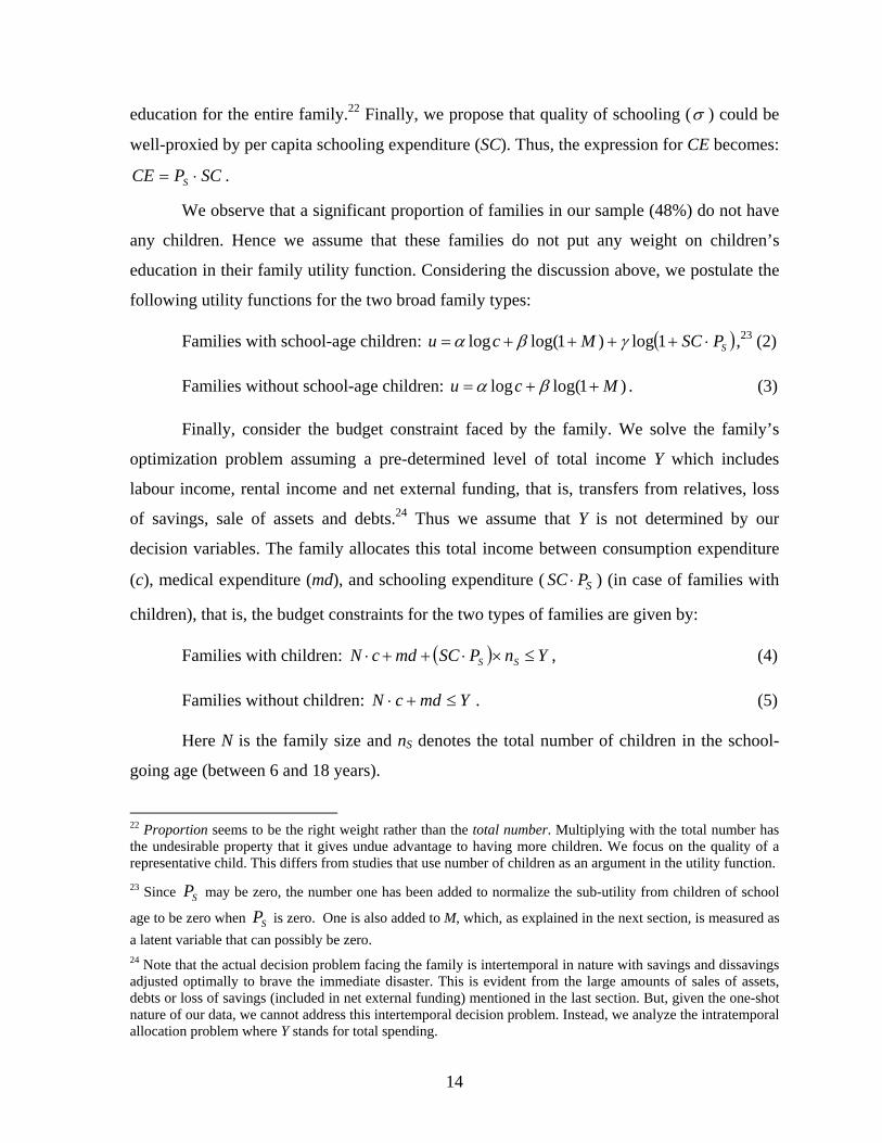
education for the entire family.22 Finally, we propose that quality of schooling (σ ) could be

well-proxied by per capita schooling expenditure (SC). Thus, the expression for CE becomes:

SCPCE S ⋅= .

We observe that a significant proportion of families in our sample (48%) do not have

any children. Hence we assume that these families do not put any weight on children’s

education in their family utility function. Considering the discussion above, we postulate the

following utility functions for the two broad family types: Families with school-age children: ( )SPSCMcu ⋅++++= 1log)1log(log γβα ,23 (2)

Families without school-age children: )1log(log Mcu ++= βα . (3) Finally, consider the budget constraint faced by the family. We solve the family’s

optimization problem assuming a pre-determined level of total income Y which includes

labour income, rental income and net external funding, that is, transfers from relatives, loss

of savings, sale of assets and debts.24 Thus we assume that Y is not determined by our

decision variables. The family allocates this total income between consumption expenditure

(c), medical expenditure (md), and schooling expenditure ( SPSC ⋅ ) (in case of families with

children), that is, the budget constraints for the two types of families are given by:

Families with children: ( ) YnPSCmdcN SS ≤×⋅++⋅ , (4) Families without children: YmdcN ≤+⋅ . (5) Here N is the family size and nS denotes the total number of children in the school-

going age (between 6 and 18 years).

22 Proportion seems to be the right weight rather than the total number. Multiplying with the total number has the undesirable property that it gives undue advantage to having more children. We focus on the quality of a representative child. This differs from studies that use number of children as an argument in the utility function. 23 Since SP may be zero, the number one has been added to normalize the sub-utility from children of school

age to be zero when SP is zero. One is also added to M, which, as explained in the next section, is measured as a latent variable that can possibly be zero. 24 Note that the actual decision problem facing the family is intertemporal in nature with savings and dissavings adjusted optimally to brave the immediate disaster. This is evident from the large amounts of sales of assets, debts or loss of savings (included in net external funding) mentioned in the last section. But, given the one-shot nature of our data, we cannot address this intertemporal decision problem. Instead, we analyze the intratemporal allocation problem where Y stands for total spending.

15

The Decision Problem of Families with Children:

{ }

( )

⎪⎪⎭

⎪⎪⎬

⎫⋅++++⋅

(4). and (1) subject to

1log)1log(log Maximize,,

SPSCmdc

PSCMcS

γβα

The first-order conditions of this optimization problem give the following three

equations which we take to the data for estimation.

,1

1⎥⎦

⎤⎢⎣

⎡+

++⋅⎟⎟

⎠

⎞⎜⎜⎝

⎛++

=⋅ SnZYcNδγβα

α (6)

,11

11 δδγβαβ ZnZYmd S

+−⎥

⎦

⎤⎢⎣

⎡+

++⋅⎟⎟

⎠

⎞⎜⎜⎝

⎛++

= (7)

,111

1

−⎥⎦

⎤⎢⎣

⎡+

++⋅⎟⎟

⎠

⎞⎜⎜⎝

⎛++

=⋅ Ss

S nZYn

PSCδγβα

γ (8)

where mdMZ ⋅−= 1δ . Decision for families without children is a special case of the

above.

5. Estimation Procedure

We estimate two different utility functions for families with school-age children and

for those without them. Table A.1 in the Appendix has the summary statistics for all the

variables used in our estimation. In each case we pool HIV and NON HIV families as we use

a currently married NON HIV family as our benchmark for welfare loss calculations. In other

words, we consider HIV families to be no different from the NON HIV families, except for

HIV status and the consequent effects on consumption, health, children’s schooling, and so

on. We describe the method for the case of families with school-age children. The method

for the case without such children is exactly the same except that there is no schooling

decision and hence one equation will be reduced.

16

5.1. Mental Health Equation

First consider the family mental health equation. Let us elaborate on the explanatory

variables clubbed under vector X in equation (1). Following the emerging literature on mental

health and subjective well-being (see, for example, Andres, 2004; Blanchflower and Oswald,

2004, 2007; Case and Deaton, 2005, 2006; Helliwell, 2006), we include wealth (W), whether

any adult family member is unemployed ( UNEMPD ), the average age of adult family members

(Av_age), the square of average age (Av_age2) and a dummy for whether there is a female

member in the family ( FEMD ). Also, considering the specific case of HIV, we include an HIV

dummy ( HIVD ) and the time span since the first detection of HIV in the family (ts). We allow

for regional differences in mental health by defining a dummy variable for the northern states

( NORTHD ) in our sample. Finally, considering the extended family structure in India and the

possibility that an HIV family may get more emotional support in an extended family, we

include a dummy variable, EXTD , to denote whether a family is a part of an extended family.

The estimable family mental health equation is assumed to be nonlinear in age and time span

since detection (ts), that is,

.__ 122

111098

7652

43210

iNORTHiiiUNEMPiEXTi

FEMiHIViiiiiii

DageAvageAvDD

DDWtstsHmdM

ωδδδδδ

δδδδδδδδ

+⋅+⋅+⋅+⋅+⋅+

⋅+⋅+⋅+⋅+⋅+⋅+⋅+= (9)

The quadratic effect of ts is meant to capture possible non-linear movement of mental health

after one finds out about HIV in the family such as an initial shock and then acceptance of

the fact or hopelessness.

Equation (9) is a technological relationship that relates how medical expenditure,

physical health and the other explanatory variables translate into mental health of the family.

Thus this equation can be estimated on its own. But before we do so, we have to deal with

the fact that the mental health index we constructed from our data is an ordinal measure,

whereas the mental health variable in equation (9) is a continuous measure. The data and our

index are reconciled by assuming that the responses of families (given by the orderings) are

based on an underlying latent mental health variable M, given in equation (9). We further

assume that the errors in equation (9) follow a normal distribution, which results in an

17

ordered probit model. Thus we estimate parameters by ordered probit.25 Using these

parameters we calculate the predicted value of M for each family. We use the predicted value

M̂ for the rest of our empirical analysis as the (continuous) measure of mental health for

each family.26

5.2. Consumption, Medical Expenditure and Schooling Equations

There are three equations to estimate the underlying parameters when SPSC ⋅ and md

are strictly positive. Define

γβααφ++

≡1 , γβα

γφ++

≡2 and γβα

βφ++

≡3 .

Then the estimable consumption, medical expenditure and schooling equations are:

,11

11 iSi

iiii nZYcN ε

δφ +⎥

⎦

⎤⎢⎣

⎡+

++⋅=⋅ (10)

,1)1( 21

2 iSii

iSiiSi nZYPSCn εδ

φ +⎥⎥⎦

⎤

⎢⎢⎣

⎡+

++⋅=⋅+⋅ (11)

ii

Sii

iiZnZYmd 311

311 εδδ

φ ++

−⎥⎦

⎤⎢⎣

⎡+

++⋅= , (12)

where iii mdMZ ⋅−= 1δ .

Equations (10), (11) and (12) form a seemingly unrelated system of equations

(SURE) for the family. However, since the three add up to income in the budget constraint,

only two of them can be used for estimation. We use equations (10) and (11). Notice that

they have the same regressors. Hence system OLS is consistent and efficient and reduces to

OLS equation by equation.

An issue of concern in using OLS is the possibility of selection bias. In the structural

model, these equations hold for positive md, c and SC.PS, so we use only the observations

25 This is in line with Blanchflower and Oswald (2004, 2007) who use ordered logit. The qualitative results do not change if we assume a logit specification. 26 Since M is an ordering, it is invariant to the constant term. We predict M based on the intercept value of zero and use (1+ M̂ ) in the utility function so that its logarithm is always defined.

18

when these conditions hold. However one can argue, a la Heckman, that these make the

estimates inconsistent. To check for that we ran the models on the full sample with Heckman

corrections but since md and SC.PS are zero for a very small proportion of our sample (about

10% for both), the estimates were almost identical. Therefore the OLS parameters are

consistent and efficient.

The OLS regressions yield 1̂φ and 2̂φ , whereas 3̂φ is derived from the restriction:

.1ˆˆˆ321 =++ φφφ For the sample without school-age children we first estimate the mental

health “technology” equation. Since there is no schooling decision, we only estimate

equation (10).

In all our estimation procedures, we pool the HIV and NON HIV sample and since

we have over-sampled HIV families as compared to their proportion in the all-India

population we use weighted least squares (and weights for probit) to correct for this possible

source of bias. Our weighting procedure is sincere to our sampling procedure. While

sampling, we sampled a family when we found out that there was an HIV infected person in

the family. We did not explicitly look to sample HIV men or women. Neither did we attempt

to sample a certain kind of family (male infected or female infected or both infected). Hence

we will assume that conditional on finding an HIV person, his/her family structure is

representative. Thus our weighting procedure takes into account the probability of finding the

main respondent who is HIV (irrespective of whether the spouse is HIV). In other words, the

weight given to a family is the weight of male HIV if the main respondent is male and vice

versa if the main respondent is female HIV. It turns out our sampling proportions of each

gender are almost similar to the population proportions given by NACO. Since we over-

sampled HIV respondents, we need to put a smaller weight on them to be truly

representative. As an example,

Weight of a family with main respondent male = sample in males HIVof Proportion

population in males HIVof Proportion .

Thus, as can be seen in Table 6, when we pool the data, any family with a HIV

respondent gets a very low weight, while NON HIV families get much higher weight. Notice

that since we have very few female respondents for NON HIV families, they have to be

weighted the most.

Also, all standard errors in the following analysis are robust.

19

6. Estimation Results

First let us look at the determinants of mental health. In the ordered probit estimation

with the full set of possible explanatory variables specified in equation (9), only a subset of

variables is statistically significant. Since we would like to use the predicted value M̂ for the

estimation of preference parameters, we conduct a joint significance of a subset of variables

that are insignificant in themselves, and, based on this Wald test, we drop the insignificant

variables and then re-estimate equation (9) with only the significant variables. The results for

both measures of mental health, 1IMH and 2IMH , are reported in Table 7.27

Since these are not the marginal effects, we only discuss the signs of the coefficients

and not the magnitudes. For both measures, better current physical health leads to better

mental health. Controlling for current physical health, the higher the medical expenditure the

higher is the mental health. This is an important result for our model. We contend that,

controlling for current physical health, people who spend more money on medical

expenditure, do so to affect their expected future health. The significant and large coefficient

on HIVD suggests that HIV infection affects mental health negatively.

The effects of other variables are specific to the measure of mental health considered.

With IMH2, we get the “U” shaped relation between mental health and age, as well

documented in the recent well-being literature. The coefficients of time span variable

suggests that, controlling for physical health, the measure based on self reported depression

gets better as more time passes and the non-linearity is not evident. Wealth affects IMH1

positively. Belonging to an extended family increases mental health (IMH1), as expected.

Presence of a female member lowers the mental health (IMH2) of the family. The basic

flavour of our results is not too different if we assume a logistic distribution instead of

normal distribution for the error term.

As mentioned earlier, we now use the ordered probit estimates to convert the ordinal

ranking in our mental health measure to a continuous quantitative measure given by the latent

variable underlying the ordered probit model. We use this continuous measure in our

empirical analysis below including the estimation of equations (10 – 12). For the remaining

27 The estimates with the full set of explanatory variables and the Wald test are reported in Das, Mukhopadhyay and Ray (2007).

20

part of the paper, we report the results using 1IMH as it uses all our questions reflecting

depression (results are similar with 2IMH ).

Table 8 reports the estimates of the parameters of the consumption and schooling

equations. The estimate of parameter relating to mental health is computed by subtracting the

sum of the reported estimates from one. The relative magnitudes confirm the observation

made by the doctors and HIV counsellors: mental health (which in turn depends on current

and expected future physical health) in the family utility function is much more important

than consumption or children’s education. For example, to keep a family (with school-age

children) at the same level of utility as would be obtained at the mean values of all variables,

per capita consumption expenditure has to be reduced by Rs. 818 if mental health is

increased by one standard deviation. This is almost equal to the mean value of per capita

consumption. This is equally true when we consider the substitution between education and

mental health. This points out to the importance of mental health in the utility function.

To get a concrete measure of welfare loss due to HIV we use these utility function

estimates to obtain a monetary equivalent value of the loss to each family in the next section.

7. Measurement of Welfare Loss

The welfare loss of the HIV/AIDS epidemic at the family level is calculated by

comparing the indirect utility functions of the HIV infected families with the NON HIV

families. Let S stand for the vector of the exogenous variables in the model:

S = (Y, H, N, nS, W, ts, DHIV, DFEM, DEXT, Av_age),

and τ denote the (hypothetical) transfer that a family receives from outside. Then the

family’s indirect utility function with this hypothetical transfer τ , )|( τSV , is defined as

{ }( )

( )⎪⎪

⎩

⎪⎪

⎨

⎧

⋅+⋅+⋅+=+≤×⋅++⋅

⋅++++

=

⋅

XHmdMYnPSCmdcN

PSCMc

SVSS

SPSCmdc S

λδδδτ

γβα

τ

210

,,

and ,s.t.

1log)1log(log Maximize

)|(

21

Consider any two families – family i with Si, and family j with Sj. If family i is the

reference family, then the amount of compensating transfer (CV) ijτ needed to bring the

family j up to the same (indirect) utility level as the reference family i is defined by: ).0|()|( i

ijj SVSV =τ

When the reference family i is an average NON-HIV family and family j is an average HIV

family, then ijτ measures the monetary equivalent of welfare loss from HIV/AIDS to an

average HIV family.

Given the Cobb-Douglas utility specification, solving the expression for ijτ for

families with school-age children yields:

.11

11⎥⎦

⎤⎢⎣

⎡+

++−⎥

⎦

⎤⎢⎣

⎡⋅⎥

⎦

⎤⎢⎣

⎡⋅⎥

⎦

⎤⎢⎣

⎡+

++=

++++ js

jj

is

js

i

ji

s

iiij nZY

nn

NNnZY

δδτ

γβαγ

γβαα

(13a)

For families without school-age children:

.11

11⎥⎦

⎤⎢⎣

⎡ ++−⎥

⎦

⎤⎢⎣

⎡⋅⎥

⎦

⎤⎢⎣

⎡ ++=

+

δδτ

βαα

jj

i

jiiij ZY

NNZY (13b)

7.1. Monetary Equivalent of Welfare Loss (CV)

Note that we have (using IMH1)

._11 2

1

11

1

8

1

6

1

5

1

2

1

0

1

ageAvDDWHZEXTHIV δ

δδδ

δδ

δδ

δδ

δδ

δ+++++

+=

+

Now, for example, consider two families i and j such that family i has no HIV

positive adult ( 0=HIVD ) whereas family j has at least one HIV positive adult member

( 1=HIVD ), and the two families are identical otherwise.28 Then (13) implies:

,039,661

6 =−=δδ

τ ij that is, “other things remaining the same”, the monetary equivalent of

the welfare loss to an HIV family is Rs. 66,039 per month.

28 That is, Yi = Yj, Hi = Hj, Ni = Nj, nSi = nSj, Wi = Wj, tsi = tsj, DEXTi = DEXTj, and Av_agei = Av_agej.

22

Similarly, consider two families i and j differing only in physical health (morbidity),

that is, ,ji HH ≠ but identical otherwise. Then (13) implies: ,652,13)( 1

2 ==−∂

∂δδτ

ji

ij

HH

implying that “other things remaining the same”, (money) value of one unit of physical

health improvement to a family is Rs. 13,652 per month.

Table 9 lists all these partial effects on compensating variation using IMH1, the

measure based on all questions. All our results henceforth are based on this measure.

7.2. Welfare Loss from HIV: the All-India Picture

Table 9 points out the partial effects on welfare loss where “other things remain the

same”. But other things do not remain the same, for example, physical health (H) obviously

deteriorates with HIV infection. Thus we are also interested in the total effect, both at the

family and all-India level, where other things are not necessarily the same. For this purpose

we consider a married NON HIV family as the reference group because widowhood,

widower-hood as well as the state of being unmarried can well be a consequence of HIV

infection.

It turns out that the total welfare loss for an average HIV family, averaging across

families with and without school going age children, is Rs. 89,008 per month. Splitting

family losses equally among infected members, the total loss amounts to Rs. 67,601 per

month for a male living with HIV/AIDS and Rs. 65,120 for a female. These figures are huge

considering the fact that the average per capita consumption expenditure of the families in

our sample is just Rs. 1,019 per month.

As a back-of-the-envelope calculation, scaling up at the all-India level, the above

figures imply that the loss to the male HIV affected population in India is Rs. 104.78 billion

per month and that for female population is Rs. 61.86 billion per month or a total of Rs.

166.64 billion per month based on a total number of 1.55 million males and 950 thousand

females living with HIV/AIDS in India (using gender proportions from UNAIDS figures).

The total welfare loss per year with just 0.36 percent of the population affected thus comes

out at Rs. 1999.8 billion, which is about one and half times the annual health expenditure of

Rs. 1,356 billion for all ailments in India in 2004 and 7% of GDP!

23

As mentioned earlier such huge magnitude is not surprising because it reflects the

private valuation of one’s life as well as the cost of stigma for being HIV positive.

Blanchflower and Oswald (2004), using a different approach also come up with similar large

figures. In the same vein, Crafts and Haacker (2004) evaluate the welfare cost of increased

mortality associated with HIV/AIDS and estimate similar large figures for welfare losses: in

Vietnam, with an adult HIV prevalence rate of only 0.4%, welfare loss already exceeds 2%

of GDP, whereas in Botswana, with 37.3% prevalence rate, the welfare loss is around 90% of

GDP.

Finally, we would like to draw attention to another source of loss to the society that

occurs due to loss of savings, sale of assets, increase in debts or increase in monetary

transfers from relatives – everything that we have clubbed under net external funding in

Table 5. We treat these as losses as these funds have alternative uses and hence represent a

drain of economic resources due to loss of labour income and increased medical expenditure.

We calculate this loss due to transfers with married NON HIV families as the reference

group. The loss per HIV male comes to Rs. 13,584 per annum while that for the female is

estimated to be Rs. 14,544 per HIV female. This amounts to Rs. 21 billion for all males and

Rs. 13.8 billion for all females. The total loss from transfers is 2.6% of the total health

expenditure of the country and 0.12% of GDP in 2004. These numbers are also quite large

given that only 0.36% of the population is infected by HIV/AIDS.

7.3. Welfare Losses across Family Types

We observed in section 3 that the ‘widow’ families could be particularly vulnerable –

they have the lowest per capita income, and the lowest proportion of school-age children

attending school. Since we have data for various different family types, it is interesting to

check whether the welfare losses differ significantly across different types of families with

HIV. For this purpose we regress the welfare losses on dummy variables reflecting different

family types. We use the Only Male HIV Married Families as the control group as it is the

most common type of HIV family. We also regress losses due to transfers (deviations of net

external funding from the level of NON-HIV Married Families) on family types.

Table 10 reports this regression result that says that the welfare loss per month is Rs.

86,217 for an average HIV family where only the male adult is infected. The loss is reduced

24

to Rs. 67,882 for an average HIV family where only the female adult is infected, and

increases to Rs. 92,284 when both adults are infected. It is important to note that the highest

loss among all family types occurs to the widow HIV families, Rs. 93,360 per month.

Clearly, the widow HIV families are in the most vulnerable situation and need careful

attention from any policy initiative. From the last column of Table 10 it is also clear that the

losses due to external funding is the highest for the unmarried females and widows.

7.4. Welfare Loss: Significance of Mental Health

In this subsection we delve a bit deeper into the determinants of welfare loss to

highlight the significance of mental health. Table 11 reports the various disaggregates of the

money equivalent expressions given in equation (13).29, 30

From Table 11 it is clear that the differences in 1

1δ

Z+ dwarfs the differences in Y

between the HIV and NON HIV families. As a matter of fact, most HIV families have higher

Y than NON HIV families. The other two variables, N and nS, do not play that big a role since

γβαγ

γβαα

++

⎥⎥

⎦

⎤

⎢⎢

⎣

⎡⋅++

⎥⎦

⎤⎢⎣

⎡i

j

i

j

snsn

NN is usually close to one as neither the average family sizes

nor the average number of school-age children are that different between the HIV and NON

HIV families. The estimates for 1

1δ

Z+ come from the mental health technology (Table 7) and

emphasize the role of mental health in our analysis.

In order to further understand the significance of different components in welfare

loss, Table 12 reports the contribution to welfare loss coming from the differences (with the

reference NON HIV married families) in two key components – physical health and HIV

status. For example, the figure 16,213 in row 2 column 2 says that for the only male HIV

29 Y is different from Income in Table 5. There the per capita income does not include transfers. It is lower than Y reported in this table. 30 In Table 11 we consider only those family types that are significant in the welfare loss regression reported in Table 10.

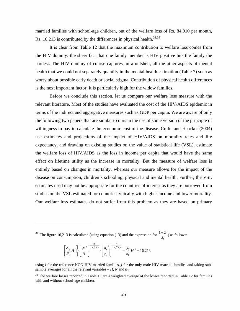
25

married families with school-age children, out of the welfare loss of Rs. 84,010 per month,

Rs. 16,213 is contributed by the differences in physical health.31,32

It is clear from Table 12 that the maximum contribution to welfare loss comes from

the HIV dummy: the sheer fact that one family member is HIV positive hits the family the

hardest. The HIV dummy of course captures, in a nutshell, all the other aspects of mental

health that we could not separately quantify in the mental health estimation (Table 7) such as

worry about possible early death or social stigma. Contribution of physical health differences

is the next important factor; it is particularly high for the widow families.

Before we conclude this section, let us compare our welfare loss measure with the

relevant literature. Most of the studies have evaluated the cost of the HIV/AIDS epidemic in

terms of the indirect and aggregative measures such as GDP per capita. We are aware of only

the following two papers that are similar to ours in the use of some version of the principle of

willingness to pay to calculate the economic cost of the disease. Crafts and Haacker (2004)

use estimates and projections of the impact of HIV/AIDS on mortality rates and life

expectancy, and drawing on existing studies on the value of statistical life (VSL), estimate

the welfare loss of HIV/AIDS as the loss in income per capita that would have the same

effect on lifetime utility as the increase in mortality. But the measure of welfare loss is

entirely based on changes in mortality, whereas our measure allows for the impact of the

disease on consumption, children’s schooling, physical and mental health. Further, the VSL

estimates used may not be appropriate for the countries of interest as they are borrowed from

studies on the VSL estimated for countries typically with higher income and lower mortality.

Our welfare loss estimates do not suffer from this problem as they are based on primary

31 The figure 16,213 is calculated (using equation (13) and the expression for 1

1δ

Z+ ) as follows:

213,161

2

1

2 =−⎥⎥⎦

⎤

⎢⎢⎣

⎡⋅

⎥⎥⎦

⎤

⎢⎢⎣

⎡⋅⎥

⎦

⎤⎢⎣

⎡ ++++ ji

s

js

i

ji H

nn

NNH

δδ

δδ γβα

γγβα

α

using i for the reference NON HIV married families, j for the only male HIV married families and taking sub-sample averages for all the relevant variables – H, N and nS. 32 The welfare losses reported in Table 10 are a weighted average of the losses reported in Table 12 for families with and without school-age children.

26

household data where we have allowed the data itself to determine the relative weights of

different components in family preferences.

The other work by Bell (2005) sets up a nice conceptual framework using the

principle of willingness to pay, captured in terms of compensating variation (CV) and

equivalent variation (EV), to evaluate the direct costs of sickness and premature adult

mortality. Unfortunately, he cannot estimate these costs as he does not have the empirical

estimates of the required parameters. Instead he estimates the EV for Kenya using a model

where there is no sickness but children’s human capital appears in the household’s

preferences. He estimates that the EV is about six to nine times the loss in GDP per young

adult.

8. Robustness

We have carried out two robustness checks to validate our exercise: first, with respect

to the choice of mental health index, and second, with respect to the choice of the utility

function.

8.1. Choice of Mental Health Index

Although we have presented most of the results using IMH1 that uses all the mental

health questions, Table 7 presents estimates of the mental health equation also with IMH2, the

index that uses responses to only one question: “I felt depressed”. The estimates somewhat

differ depending on which index one uses. But the significance and magnitudes of the key

variables like md, H and DHIV are not very different so that when we use the estimates to

calculate the welfare losses, the figures turn out to be very similar. For example, using IMH2,

the welfare loss is estimated to be Rs. 76,986 per month for a male living with HIV/AIDS

and Rs. 84,272 for a female (recall that the respective figures using IMH1 are Rs. 67,601 for

males and Rs. 65,120 for females). Note that, using IMH2, welfare loss per female is higher

whereas loss per male is lower (compared to using IMH1). The reason is that the coefficient

of the female dummy is negative and significant (with a relatively high magnitude) in IMH2,

but insignificant in IMH1.

27

As a robustness check, we use another measure of mental health which is cardinal –

the proportion of all questions wherein the family said that it was “Never” in the bad mental

state. The costs, using this index are Rs. 58,289 per male and Rs. 54,352 per female.

8.2. Choice of the Utility Function

Since the analysis has been done using a Cobb-Douglas utility function, a natural

question that emerges is how sensitive the results are to an alternative specification of the

utility function. We redo our exercise with Constant Elasticity of Substitution (CES) utility

function for the general model and get very similar results.33 The loss (using IMH1) per

month for a HIV male is Rs. 68,163 and for a HIV female is Rs. 65,729. Recall that the

corresponding figures with the Cobb-Douglas utility function are Rs. 67,601 and Rs. 65,120

respectively. Thus our earlier results are robust.

The reason for the robustness lies in the fact that in almost all specifications in this

family of CES utility functions, when calculating the money equivalent, the main loss comes

from 1

1δ

Z+ . The money equivalent expression for CES function is given by

.11

1

1

111

111

1

1

111

1

⎥⎦

⎤⎢⎣

⎡+

++−⎥

⎦

⎤⎢⎣

⎡+

++⋅

⎥⎥⎥

⎦

⎤

⎢⎢⎢

⎣

⎡

⎟⎟⎠

⎞⎜⎜⎝

⎛⋅+⎟

⎠

⎞⎜⎝

⎛⋅+⎟⎟

⎠

⎞⎜⎜⎝

⎛⋅

⎥⎥⎥

⎦

⎤

⎢⎢⎢

⎣

⎡

⎟⎟⎠

⎞⎜⎜⎝

⎛⋅+⎟

⎠

⎞⎜⎝

⎛⋅+⎟⎟

⎠

⎞⎜⎜⎝

⎛⋅

= −

−−−

−

−−−

jS

jji

S

ii

jS

j

iS

i

ij nZYnZY

nN

nN

δδ

γγ

βδβ

αα

γγ

βδβ

αα

τρρ

ρρ

ρρ

ρρ

ρρ

ρρ

ρρ

ρρ

Note that in this expression, the first part of the first term is close to one as neither the

average family sizes nor the average numbers of school-going children are that different

between the HIV and NON HIV families. This implies that, once again, the differences in Y

and 1

1δ

Z+ determine the loss. As before differences in 1

1δ

Z+ is the dominant component of

the loss and hence the results are similar.

33 The details of the CES estimation are available from the authors on request.

28

9. Concluding Remarks

HIV/AIDS is of serious concern both locally and globally. According to the latest

available estimates, about 2.5 million people in India are currently living with HIV or AIDS.

This paper calculates the cost of HIV/AIDS by estimating directly the monetary equivalent of

welfare loss at the individual/family level for the people currently living with HIV/AIDS. We

consider a new channel through which HIV/AIDS affects family welfare, namely, the loss of

mental health. Using the methodology suggested in Das, Mukhopadhyay and Ray (2007),

which integrates mental health in welfare evaluation by allowing for proper substitution

possibilities in the family preferences, we value the monetary loss taking into account this

new channel.

We use primary household data from India and estimate household utility function

parameters that measure the relative importance of consumption, schooling of children and

mental and physical health effects of HIV/AIDS in India. We find that mental health effects

are far more important than the effect of consumption or children’s schooling in determining

utility. Using a compensating variation approach and using a NON HIV “married” family as

the reference group, we find that the loss to an HIV family amounts to Rs. 66,039 per month.

This loss is the maximum in case of widows. Clearly, the widow HIV families are in the

most vulnerable situation and need careful attention from any policy initiative. The

maximum contribution to welfare loss comes from worry about possible early death or social

stigma. The loss of physical health is the next important factor in explaining welfare loss. We

also find that, for HIV households, consumption is funded through transfers from other

family members, sale of assets and dissavings. These are funds lost for other productive

purposes. The aggregate total loss from these funds is 2.6% of the total health expenditure of

the country and 0.12% of GDP in 2004.

Our analysis suggests that loss of mental health constitutes 74% of the total welfare

loss. Our work is unique in that, while it is well known that terminal illnesses lead to despair

and depression, this paper is the first to attempt to quantify such losses in the case of

HIV/AIDS. The large impact of mental health implies that studies that do not take into

account this channel of impact may miss the dimension on which individuals and families are

most affected.

29

References

[1] Arndt, C. and Lewis, J.D. (2000), “The Macro Implications of HIV/AIDS in South

Africa: A Preliminary Assessment,” South African Journal of Economics, 856-87.

[2] Andres, A.R. (2004), “Determinants of Self-reported Mental Health Using the British

Household Panel Survey,” Journal of Mental Health Policy and Economics, vol. 7(3),

99-106.

[3] Bell, C. (2005), “Estimating the Costs of Sickness and Premature Adult Mortality,”

mimeo, South Asia Institute, University of Heidelberg.

[4] Bell, C., Devarajan, S. and Gersbach, H. (2004), “Thinking about the Long-Run

Economic Costs of AIDS,” in The Macroeconomics of HIV/AIDS, ed. by Markus

Haacker, Washington DC: International Monetary Fund.

[5] Bell, C., Devarajan, S. and Gersbach, H. (2006), “The Long-run Economic Costs of

AIDS: Theory and an Application to South Africa,” World Bank Economic Review,

vol. 20, 55-89.

[6] Blanchflower, D.G. and Oswald, A.J. (2004), “Well-being over Time in Britain and the

USA,” Journal of Public Economics, vol. 88, 1359-86.

[7] Blanchflower, D.G. and Oswald, A.J. (2007), “Is Well-being U-shaped over the Life

Cycle?” NBER Working Paper No. 12935.

[8] Bloom, D.E. and Mahal, A.S. (1997), “Does the AIDS Epidemic Threaten Economic

Growth?” Journal of Econometrics, 105-24.

[9] Bonnel, R. (2000), “HIV/AIDS and Economic Growth: A Global Perspective,” South

African Journal of Economics, 820-55.

[10] Booysen, F. le R. and Bachmann M. (2002), “HIV/AIDS, Poverty and Growth:

Evidence from a Household Impact Study Conducted in the Free State Province,

South Africa,” Paper presented at the Annual Conference of the Centre for the study

of African Economies, Oxford, March 18-19.

[11] Case, A. and Deaton, A. (2005), “Health and Wealth among the Poor: India and South

Africa Compared.” American Economic Review Papers and Proceedings, 229-233.

30

[12] Case, A. and Deaton, A. (2006), “Health and Well-Being in Udaipur and South

Africa,” in Developments in the Economics of Aging, ed. by D. Wise, University of

Chicago Press (forthcoming).

[13] Corrigan, P., Glomm, G. and Mendez, F. (2005), “AIDS Crisis and Growth,” Journal

of Development Economics, 107-24.

[14] Corrigan, P., Glomm, G. and Mendez, F. (2004), “AIDS, Human Capital and Growth,”

mimeo.

[15] Crafts, N. and Haacker, M. (2004), “Welfare Implications of HIV/AIDS,” in The

Macroeconomics of HIV/AIDS, ed. by Markus Haacker, Washington DC:

International Monetary Fund.

[16] Cuddington, J.T. (1993a), “Modeling the Macroeconomic Effects of AIDS with an

Application to Tanzania,” World Bank Economic Review, 173-89.

[17] Cuddington, J.T. (1993b), “Further Results on the Macroeconomic Effects of AIDS:

The Dualistic Labor-Surplus Economy,” World Bank Economic Review, 403-17.

[18] Cuddington, J.T. and Hancock, J.D. (1994), “Assessing the Impact of AIDS on the

Growth Path of the Malawian Economy,” Journal of Developing Economics, 363-68.

[19] Das, S., Mukhopadhyay, A. and Ray, T. (2007), “Integrating Mental Health in Welfare

Evaluation: An Empirical Application,” Discussion Paper 07-06, Indian Statistical

Institute, Delhi.

[20] Deininger, K., Garcia M. and Subbarao K. (2003), “AIDS-Induced Orphanhood as a

Systemic Shock: Magnitude, Impact and Program Interventions in Africa,” World

Development, 1201-1220.

[21] Emanuel, E.J., Fairclough, D.L., Slutsman, J. and Emanuel, L.L. (2000),

“Understanding Economic and other Burdens of Terminal Illness: The Experience of

Patients and their Caregivers,” Annals of Internal Medicine, vol. 132, 451-59.

[22] Evans, D. and Miguel, E. (2005), “Orphans and Schooling in Africa: A Longitudinal

Analysis,” Working Paper No. C05-143, Centre for International and Development

Economics Research, University of California, Berkeley.

[23] Ferreira, C.P. and Pessoa, S. (2003), “The Long-Run Impact of AIDS,” mimeo,

Graduate School of Economics, Fundacao Getulio Vargas, Rio de Janeiro.

31

[24] Gertler, P., Martinez, S., Levine, D. and Bertozzi, S. (2003), “Losing the Presence and

Presents of Parents: How Parental Death Affects Children,” mimeo.

[25] Graham, C. (2007), “The Economics of Happiness,” in The New Palgrave Dictionary

of Economics, eds., S. Durlauf and L. Blume, Second Edition (forthcoming).

[26] Grunfeld, E., Coyle, D., Whelan, T., Clinch, J., Reyno, L., Earle, C.C., Willan, A.,

Viola, R., Coristine, M., Janz, T. and Glossop, R. (2004), “Family Caregiver Burden:

Results of a Longitudinal Study of Breast Cancer Patients and their Principal

Caregivers,” Canadian Medical Association Journal, 170 (12), 1795-801.

[27] Haacker (2004), “HIV/AIDS: The Impact on the Social Fabric and the Economy,” in

The Macroeconomics of HIV/AIDS, ed. by Markus Haacker, Washington DC:

International Monetary Fund.

[28] Helliwell, J.F. (2006), “Well-being, Social Capital and Public Policy: What’s New?”

Economic Journal, vol. 116, C34-C45.

[29] International Institute for Population Sciences (IIPS), 2007, “2005-2006 National

Family Health Survey (NFHS-3) – National Fact Sheet India (Provisional Data)”

(Deonar, Mumbai: IIPS).

[30] Kambou, G., Devarajan, S. and Over, M. (1992), “The Economic Impact of AIDS in an

African Country: Simulations with a General Equilibrium Model for Cameroon,”

Journal of African Economies, 109-30.

[31] McDonald, S. and Roberts, J. (2006), “AIDS and Economic Growth: A Human Capital

Approach,” Journal of Development Economics, 228-250.

[32] Sherman, D.W. (1998), “Reciprocal Suffering: The Need to Improve Caregiver’s

Quality of Life Through Palliative Care”, Journal of Palliative Medicine, 357-366.

[33] Sen, A. (1986), “Social Choice Theory”, in Handbook of Mathematical Economics, ed.

by K. J. Arrow and M. D. Intriligator, North-Holland, vol. 3, 1073-1181.

[34] Yamano, T. and Jayne, T.S. (2005), “Working-Age Adult Mortality and Primary

School Attendance in Rural Kenya,” Economic Development and Cultural Change,

619-653.

[35] Young, A. (2005), “The Gift of the Dying: The Tragedy of Aids and the Welfare of

Future African Generations,” Quarterly Journal of Economics, 423-66.

32

Figure 1: Age Distribution

0.000.050.100.150.200.250.300.35

0-5 6-10 11-14 15-18 19-24 25-30 31-35 36-40 41-45 46-49 50+

Age Groups

Prop

ortio

n

Proportion of HIV Positive Individuals Proportion of HIV Positive Males Proportion of HIV Positive Females

Figure 2: Time Since Detection of HIV

0.000.050.100.150.200.250.300.350.40

Less than 0.5 0.5-1 1-2 2-4 4-7

Years

Prop

ortio

n

Proportion of HIV Positive Individuals Proportion of HIV Positive Males Proportion of HIV Positive Females

33

Table 1: Family Types

Proportion

Family Types HIV NON HIV

Currently Married 0.61 0.71

Never married 0.14 0.22

Ever Married 0.25 0.07

Table 2: Physical Health Index

Health index

HIV

Male: 7.8 (1.8)

Female: 8.6 (1.9)

Average Family 8.5 (1.5)

NON HIV

Male: 10.3 (1.1)

Female: 10.5 (0.9)

Average Family 10.3 (0.8)

(Standard errors are in the parentheses.)

34

Table 3: Mental Health: Relative Frequency (in %)

HIV families

IMH1 IMH2

NON HIV families

IMH1 IMH2

Most of the time (1) 82.43 57.77 37.74 5.76

Sometimes (2) 14.05 28.34 17.82 15.57

Hardly Ever (3) 3.24 7.36 24.95 23.67

Never (4) 0.27 6.54 19.50 55.01

Table 4: Effect on Children’s Education

Proportion Attendance (Ps)

(Age: 6-18)

Quality Adjusted

Attendance (SC.PS)

HIV Families

Widow 0.74 (0.40) 71 (119)

Widower 0.75 (0.43) 106 (156)

Currently Married 0.93 (0.23) 152 (234)

NON HIV families 0.89 (0.27) 132 (154)

(Standard errors are in the parentheses.)

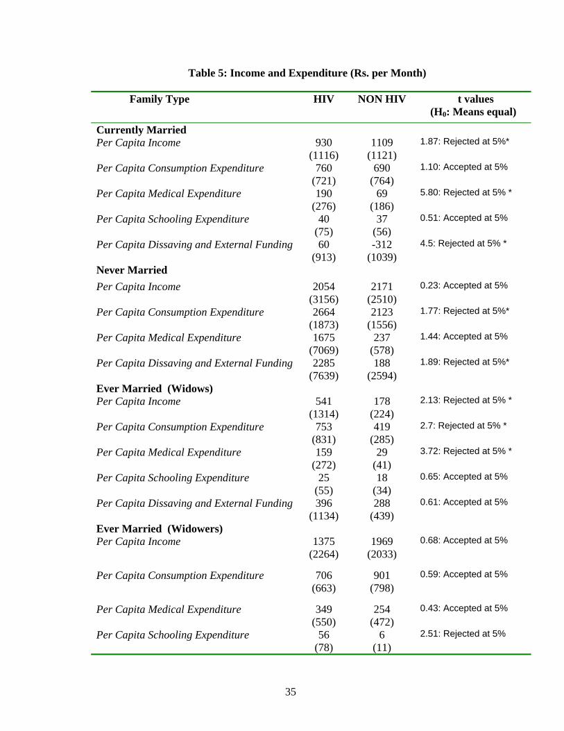
35

Table 5: Income and Expenditure (Rs. per Month)

Family Type HIV NON HIV t values (H0: Means equal)

Currently Married Per Capita Income 930

(1116) 1109

(1121) 1.87: Rejected at 5%*

Per Capita Consumption Expenditure 760

(721) 690

(764) 1.10: Accepted at 5%

Per Capita Medical Expenditure 190

(276) 69

(186) 5.80: Rejected at 5% *

Per Capita Schooling Expenditure 40 (75)

37 (56)

0.51: Accepted at 5%

Per Capita Dissaving and External Funding 60 (913)

-312 (1039)

4.5: Rejected at 5% *

Never Married Per Capita Income 2054

(3156) 2171

(2510) 0.23: Accepted at 5%

Per Capita Consumption Expenditure 2664 (1873)

2123 (1556)

1.77: Rejected at 5%*

Per Capita Medical Expenditure 1675 (7069)

237 (578)

1.44: Accepted at 5%

Per Capita Dissaving and External Funding 2285 (7639)

188 (2594)

1.89: Rejected at 5%*

Ever Married (Widows) Per Capita Income 541

(1314) 178

(224) 2.13: Rejected at 5% *

Per Capita Consumption Expenditure 753

(831) 419

(285) 2.7: Rejected at 5% *

Per Capita Medical Expenditure 159

(272) 29

(41) 3.72: Rejected at 5% *

Per Capita Schooling Expenditure 25

(55) 18

(34) 0.65: Accepted at 5%

Per Capita Dissaving and External Funding 396 (1134)

288 (439)

0.61: Accepted at 5%

Ever Married (Widowers) Per Capita Income 1375

(2264) 1969

(2033) 0.68: Accepted at 5%

Per Capita Consumption Expenditure 706 (663)

901 (798)

0.59: Accepted at 5%

Per Capita Medical Expenditure 349 (550)

254 (472)

0.43: Accepted at 5%

Per Capita Schooling Expenditure 56 (78)

6 (11)

2.51: Rejected at 5%

36

Per Capita Dissaving and External Funding -264 (1207)

-808 (1351)

0.96: Accepted at 5%

*(One tail test :HA | Mean1- Mean2| > 0)

Table 6: Weights

POPULATION Number/ Frequency A. Total Population 15-49 521397817 B. Number of HIV positive adult males 1550000 C. Number of HIV positive adults females 950000 D. Total Number of HIV positive adults 2500000 E. Prob of meeting a adult HIV male (B/A) 0.002972778 F. Prob of meeting an adult HIV females (C/A) 0.001822025 G Prob of meeting an adult NONHIV male 0.514800642 H Prob of meeting an adult NONHIV female 0.480404555 SAMPLE I Proportion of respondent HIV positive adult males 0.298823529 J Proportion of respondent HIV positive adults females 0.137647059 K Proportion of respondent NON HIV adult males 0.448235294 L Proportion of respondent NON HIV adults females 0.115294118 WEIGHTS M Weight on HIV positive adult male (E/I) 0.009948273 N Weight on HIV positive adult female (F/J) 0.013236936 O Weight on NON HIV adult male (G/K) 1.14850537 P Weight on NON HIV adult female (H/L) 4.166774197

37

Table 7: Mental Health: Ordered Probit Estimates

1IMH 2IMH

md 0.000018** 0.000016*

H 0.248*** 0.172***

ts 0.098**

W 0.00000146***

HIVD -1.20*** -1.73***

FEMD -0.71***

EXTD 0.68***

Av_age -0.87**

Av_age2 0.0002* 0.001**

NORTHD -0.26*

No. of Observations 829 833#

Log Pseudo Likelihood -432.92 -799.60 2χ 181.90*** 369.79***

Pseudo R2 0.10 0.09 (*** significant at 1%, ** significant at 5% and * significant at 10%) #: No. of Observations differ due to missing data.

Table 8: Estimates from Consumption, Schooling and the Transformed Medical Expenditure Equation

With School Age-Children

(ns > 0)

With School Age-Children

(ns > 0)

Without School Age- Children

(ns = 0)

1̂φ 0.014*** 0.0172***

2̂φ 0.002*** No. of Observations 326 326 348

R2 0.68 0.49 0.67 (*** significant at 1%)

38

Table 9: Partial Effects on CV ( ijτ )

Partial Effects

ji HH −

13,652

ji WW − 0.08

HIVD -66,039

EXTD 37,600

Av_agei – Av_agej 24.52

Table 10: OLS Regression: Welfare Losses and Losses from Transfers on Family Types

Welfare Loss Per Month

(Rs.)

Losses from Transfers Per Month

(Rs.) Coefficients Coefficients

Constant 86,217*** 1,420***

Only Female HIV Married Families -18,335** -1,027***

Both HIV Married Families 6067* -150

Widow HIV Families 7,143* 685**

Widower HIV Families -4,756 -520

Never Married Male Families 701 1,031

Never Married Female Families -176 1,195**

No. of Observations 369 369

R2 0.03 0.02 (*** significant at 1%, ** significant at 5% and * significant at 10%)

39

Table 11: Disaggregates of Monetary Equivalent of Welfare Losses

Y N ns

1

1δ

Z+

Average HIV Family 3000 2.93 1.01 144,047

With School-Age Children

NON HIV Married Families 2,410 4.41 2.13 231,133

Only Male HIV Married Families 2,593 4.05 2.01 146,485

Only Female HIV Married Families 2,587 3.83 1.83 162,066

Both HIV Married Families 3,176 4.00 1.80 141,425

Widow HIV Families 2,149 3.21 1.85 136,664

Without School-Age Children

NON HIV Married Families 2,639 2.60 0 239,028

Only Male HIV Married Families 2,879 2.67 0 151,760

Only Female HIV Married Families 3,825 2 0 170,122

Both HIV Married Families 3,442 2.8 0 143,869

Widow HIV Families 1,676 1.45 0 143,988

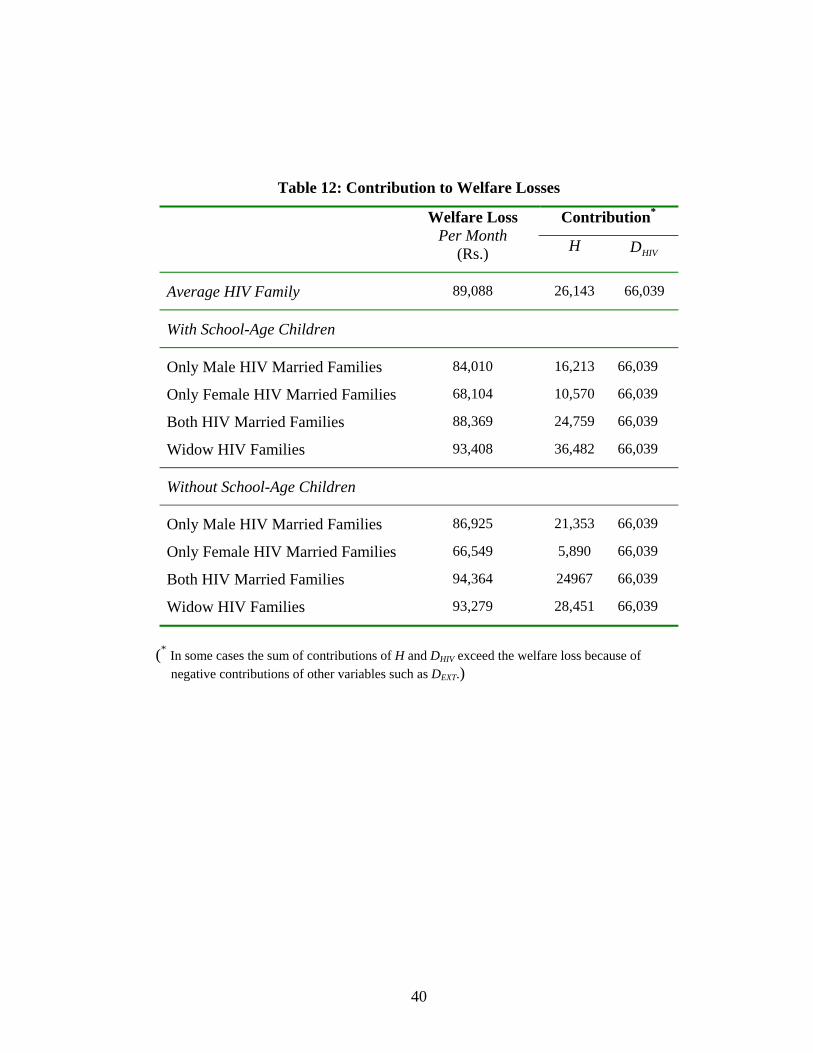
40

Table 12: Contribution to Welfare Losses

Contribution* Welfare Loss Per Month

(Rs.) H HIVD

Average HIV Family

89,088

26,143

66,039

With School-Age Children

Only Male HIV Married Families

84,010

16,213

66,039

Only Female HIV Married Families 68,104 10,570 66,039

Both HIV Married Families 88,369 24,759 66,039

Widow HIV Families 93,408 36,482 66,039

Without School-Age Children

Only Male HIV Married Families

86,925

21,353

66,039

Only Female HIV Married Families 66,549 5,890 66,039

Both HIV Married Families 94,364 24967 66,039

Widow HIV Families 93,279 28,451 66,039

(* In some cases the sum of contributions of H and DHIV exceed the welfare loss because of negative contributions of other variables such as DEXT.)

41

Appendix

Table A.1: Summary Statistics (money values in Rupees and time in years)

Mean Std Dev.

Per Capita Monthly Consumption Expenditure (c ) 1,019 1,189

Quality Adjusted School Attendance (PS. SC) 70 170

Medical Expenditure (md) 591 2,748

Family Size (N) 2.9 1.38

Average Physical Health of Family (H) 8.5 1.44

Time Span since HIV Detection (ts) 2.07 1.71

Square of Time Span since HIV Detection ( 2ts ) 7.23 9.5

Wealth (W) 18,634 50,168

Number of School Going Age Children (ns) 1.04 1.24

Family Resides in North India ( NORTHD ) 0.52 0.49

Family has Female Adult Member ( FEMD ) 0.80 0.39

Patient Lives in an Extended Family ( EXTD ) 0.63 0.48

Family has at least one Unemployed Adult ( UNEMPD ) 0.12 0.32

Average Age of Adult Members (Av_age) 32.4 8.7

Square of Average Age of Adult Members (Av_age2) 1,125 659