NBER WORKING PAPER SERIES SOLVING SYSTEMS OF NONLINEAR EQUATIONS BY BROYDEN'S METHOD WITH PROJECTED UPDATES David M. Gay* Robert B. Schnabel** Working Paper No. 169 COMPUTER RESEARCH CENTER FOR ECONOMICS AND MANAGEMENT SCIENCE National Bureau of Economic Research, Inc. 575 Technology Square Cambridge, Massachusetts 02139 March 1977 Preliminary NBER working papers are distributed informally and in limited numbers. This report has not undergone the review accorded official NBER publications; in particular, it has not yet been submitted for approval by the Board of Directors. *NBER Cc'mputer Research Center. Research conducted in part during a visit to the Atomic Energy Research Establishment, Harwell, England, and supported in part by National Science Foundation Grant MCS76-00324 to the National Bureau of Economic Research, Inc. **Computer Science Dept., Cornell University. Research conducted in part during a visit to the Atomic Energy ResearCh Establishment, ilarwell, England, and supported in part by a National Science Foundation Graduate Fellowship.

Welcome message from author
This document is posted to help you gain knowledge. Please leave a comment to let me know what you think about it! Share it to your friends and learn new things together.
Transcript
NBER WORKING PAPER SERIES
SOLVING SYSTEMS OF NONLINEAR EQUATIONS BY
BROYDEN'S METHOD WITH PROJECTED UPDATES
David M. Gay*
Robert B. Schnabel**
Working Paper No. 169
COMPUTER RESEARCH CENTER FOR ECONOMICS AND MANAGEMENT SCIENCENational Bureau of Economic Research, Inc.
575 Technology SquareCambridge, Massachusetts 02139
March 1977
Preliminary
NBER working papers are distributed informally and in limited
numbers.
This report has not undergone the review accorded official NBER
publications; in particular, it has not yet been submitted for
approval by the Board of Directors.
*NBER Cc'mputer Research Center. Research conducted in part during
a visit to the Atomic Energy Research Establishment, Harwell,
England, and supported in part by National Science FoundationGrant MCS76-00324 to the National Bureau of Economic Research, Inc.
**Computer Science Dept., Cornell University. Research conducted in
part during a visit to the Atomic Energy ResearCh Establishment,ilarwell, England, and supported in part by a National Science
Foundation Graduate Fellowship.

Abstract
We introduce a modification of Broyden's method for finding
a zero of n nonlinear equations in n unknowns when analytic
derivatives are not available. The method retains the local
Q—superlinear convergence of Broyden's method and has the addi-
tional property that if any or all of the equations are linear,
it locates a zero of these equations in n+1 or fewer iterations.
Limited computational experience suggests that our modification
often improves upon Eroyden's method.

—ii—
CONTENTS
Section Page
1. Introduction 1
2 . The Ne'q Method 5
3. Behavior on Linear or Partly Linear Problems.... 17
4. Local Q—Superlinear Convergence on NonlinearProblems 25
5. Computational Results 34
6. Summary and Conclusions 39
7. References 40

1. Introduction
This paper is concerri& with solving the prob1n
given a differentiable F(1.1)
find x' c such that F(x*) = 0
when derivatives of F axe either inconvenient or very costly to compute.
We denote the n component functions of F by
i1,...,naf.
and the Jacobian matrix of F at x by F'(x), F'(x) = (x).
When F' (x) is cheaply available, a leading method for the solution
of (1.1) is Newton's method, which produces a series of approximations
{x1 ,x2,. . . } to x by starting from approximation x0 and using the
foxrctula
X11 x1— F' (x)F(x) . (1.2)
If F is nonsingular and Lipschitz continous at x' arid x0 is
sufficiently close to x*, then the algorithm converges Q-quadratically to— i.e., there exists a constant C such that
I
- x* I c I lxi — x* 2
for all i and sanevector norm 1.11 (c.f. 59.1 of [Ortega & Rheinholdt,
1970]). If F is linear with nonsingular Jacobian matrix, then x1 = x.When F' (x) is not readily available, an obvious strategy is to replace
F'(xi)
in (1.2) by an approximation B. This leads to the irodified Newton
iteration

—2—
x. =x. -BF(x.) (1.3a)i+1 1 1 1
B÷i = tJ(B.) (1.3b)
where U is sara update formula that uses current information ahout F.
Broyden [1965] introduced a family of update formulae U known as
quasi-Newton updates. He also proposed the particular update used in
"Broyden' s method", which we consider in ITore detail below. If x0 issufficiently close to x, the matrix norm of - F' (x0) is sufficientlysnail and several reasonable conditions on F are met, then Broyden 's
method converges Q-superlinearly to x i.e.,
Hx _x*j = 0 [Broyden, Dennis & ré, 1973]. However forHx _x*I
linear F, convergence may take as many as 2n steps—and B - F' (x*)
may have rank n—i (see [Gay, 1977]).
In this paper, we introduce a new method of form (1.3) using an update
(1. 3b) which is different fran but related to Broyden' s update. Our new
method is still locally Q—superlinearly convergent under the conditions for
which Broydeth method is. It has the additional property that if F is] inear with nonsingular Jacobian matrix, then x = x for some i < n+l, and
if k+1 iterations are required ,then 3k+1 - F' (x*) has rank n-k.
Initial tests show our method to be somewhat superior in performance to
Broyden's method.
—3—
The basic idea behind our new method is related to one originally proxDsed
by Garcia-Palamares [1973]. Davidon [1975] used. this idea independently
in deriving a new method for the unconstrained minimization problem,
mm f(x) nXEn 'Davidon also ncdified an existing update formula to produce a quasi-Newton
method which does not use exact line searches but is exact on cuadratic
problems. This new method has been an irrprovement in practice. While it
has not yet been shown to retain the local superlinear convergence of lie
method it rrcclifiecl, Schnabel (1977] uses the techniques of this paper to show
that a very similar rrcdification retains Q-superlinear convergence as well
as the proper-ties of Davidon's [1975] method.
In Section 2 we briefly describe Broyden' s method and the iTrtant
features of quasi-Newton methods. We then introduce our new algorithm in
to forms: Algorithm I, a simplified version which is sufficient to dis-
cuss its basic and linear properties, and Algorithm II, the version used in
practice and to prove local superl±near convergence. We also derive the
basic properties of our method which we will use in subsequent sections.
In Section 3 we discuss the behavior of our algorithm on linear problems.
We show that if any or all of the equations f. are linear, then our new
algorithm will find a zero of these equations in n+l or fewer iterations.
We also discuss the effect of a certain restart procedure on our algorithm.
In Section 4 we show that our new method is locally Q-superlinearly con-
vergent on a wide class of problems. We discuss our computational results in
Section 5 and untrarize our results in Section 6.

—4—
Ilenceforth, I will denote the 2.2 vector norm
2 1/2 ,v )T or the ccrrescring(IIvII=(z v.) for v=(vi=1 1'.. '1
matrix norm, while 'will denote the Frcbenius matrix norm:
nfl 21/2I I I I
= ( E in. .) for i = (rn.)F1=1 j=1

—5—
2. The New Method
asi-Newton methods are often damped: they take the form
x÷1 = x — F(x) (2.la)
= U(B)(2.lb) -
where the damping factor > 0 is chosen to pratte convergence from
starting points x0 which may lie outside the region of convergence of
the corresponding direct prediction method (1.3). When it leads to a
"successful" step, e.g. reduction of I F , the choice 1 isusually preferred.
Broyden' s ("good") method is a method of form (2 .1), using the update
equation
T(y1 — Bs) s= B +
Siwhere (2.2)
Si = Ax = x1 —
x1 , (2.3a)
= =F(x÷1)
- F(x) . (2.3b)
Because of equation (2.2), B1 satisfies B÷1 bc1 = . Since
for 1l , F' (x÷1) tax. AF , we expect that B1 resth1es
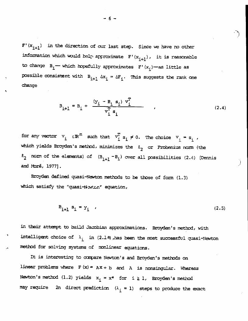
—6—
F' (x1+i) in the direction of our last step. Since we have no other
infoirnation which uld help apçroxirnate F' (x.1), it is reasonable
to change B— which hopefully approximates '(xi)—as little aspossible consisnt with B+i . = This suggests the rank one
change
(y1 - B. s1) VT3i+1 = B1
+ 1, (2.4)
for any vector v such that vT s o. The choice V S
which yields Broyden' s method, minimizes the £2 or Froberilus norm (theZ2 norm of the e1ents) of (B+i -B) over all possibilities (2.4) [Dennis
)and 1977].
Broyden defined quasi—Newton methods to be those of form (1.3)
which satisfy the "quasiNsc.n' equation,
B÷1 s = y1 , (2.5)
in their attanpt to build Jacobian approximations. Broyden'S method, with
intelligent choice of A1 in (2.1 a) ,has been the rrost successful quasi-Newton
method for solving systEns of nonlinear equations.
It is interesting to canpare Newton' s and Broyden' s methods on
lineer prob1ns where F (x) = AX + b and A is nonsingular. WhereasNewton' s method (1.2) yields x1 = x* for i 1, Broyden 's method
may require 2n direct prediction (A = 1) steps to produce the cact
—7--
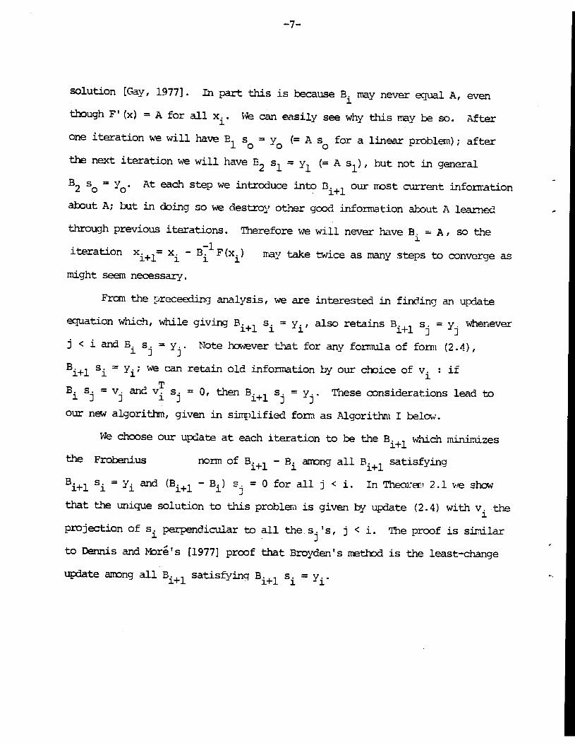
solution [Gay, 1977). In part this is because B. may never equal A, eventhough F' (x) = A for all x1. We can easily see why this may be so. Afterone iteration we will have s0 = y (= A S for a linear problem); afterthe next iteration we will have 132 S1 =
y1 (= A s1), but not in general
B2 S0=
y0. At each step we introduce into 13i+1 our irost current informationabout A; but in doing so we destroy other good information about A learned
through previous iterations. Therefore we will never have B A, SO theiteration x1= x. - B1 F (xi) may take twice as many steps to converge as
might seem necessary.
From the receeding analysis, we are interested in finding an update
equation which, while giving B.1 s = also retains B÷1 s = y. whenever
j < i and B s = Note however that for any formula of form (2.4),
B.1 S1 = y1; we can retain old information by our choice ofv1 if
B. s = v and v' s = 0, then •÷l s. = y. These considerations lead to
our n algorithm, given in simplified form as Algorithm I below.
We choose our update at each iteration to be the B11 which rniniraizes
the Frobenius norm of B.1 - B aring all 1+l satisfyingB.1 s = and (B1 — B1)
s. = 0 for all j < i. In Theo:r 2.1 we showthat the unique solution to this problem is given by update (2.4) with v theprojection of Si perpendicular to all the Si 's, < i. The proof is similar
to Dennis and vbrts [1977] proof that Broyden's method is the least-change
update arrong all B11 satisfying B1 s = y.

—8—
Thrn 2.1 Let B ar s, y be In-zero vectors C
with Bg y. Let Z be an in dimensional subspace of :IR , in < n.
Then for I I I I either the L2 or the Frobenius nonn, a
solution to
rain {B — B ItBS = y, (B — B)z=O for all z C Z} (2.6)
is
A (y-Bs)vBB+ Tvswhere v is the ort1gorial projection of s onto the ort1gonal canp1nt
of Z, i.e.,
Tin S Z.1VS Ti=1 z 1
with (z11.. Z) an ortrgonal basis for Z. The solution is unique in
the Frobenius norm.
Proof: Let S={BBsy, (B-B) z0 ZCZ}. Naw Bs=y;
ansince T=o for i=1,...,m, vT=o forall zCZ.
Thus B C S.
Now consider any B c S. Since y 35
AB—B= — sv
vT s

—9—
m TiDefine d = Z '!' z. = s - v. Since d c Z and v is perpendicular to Z,
i=1 zz. 111d = o. mus = Since ( - B) z = 0 for all z c Z, (B - B)d = 0,
so ( - B) s = ( - B)v. Therefore (B - B) = (fl-B)T so forN the
v.&.vor Frobex-ijus norm,
TlB - BuN - IIN lll ll - B
'S
Thus B is a solution to (2.). It is the uniciue solution in the Frobenius
norm because the function 5: JR - JR given by (B) = - is
strictly convex over all B in the convex set S. •
AlgorithTl I
Let x JRfl, B c F + JR11 be given.0 0
For i=0, 1, 2,...
c1ose nonzero s. E JRfl (likely s. = -x n F(x))11
x. = x. + s. (2.7a)i+1 1 1
If F(x. ) = 0 then stopi+l
y. = F(x. ) - F(x.) (2.7b)1 i+l 1

—10—
Ai—i S. S.
Q= E AT (2.7c)j=O S Si
S. = S. — C).s. 2.7)1 1 11
(y. — .s.) s.B — ÷ — 11 1i+l j ATS. S.1 1
Alçcrithn i is unsuitable for crtuter irLplerrentatiorl for several
reasons—— rrost inirtaritly; if i > n, then s. will be zero vector. However,
it is sufficient for deriving the basic properties of our algorithu (for
general functions F) in Theor 2,2 below; and is also sufficient for dis-
cussing the bebavior of our algorithn on linear problns in Section 3.
We use tJ'ie tation <a,b> to denote the scalar product
rrab = E a.b. , a, bi=l 1 1
TheorEn 2.2 Given P , B P , F P - P, let the sequences
{s0,... ,s}, y0,. .. , y}, {B01. . . , B1} be generated by Algorithm I.
Define .. ,s. as in Algorithm I and let y = y -BQs1 j = 0,. . . i.
Then at each iteration i, if se;. . . ,s. are linearly independent, then 3i+lis well defined and
— 11 —
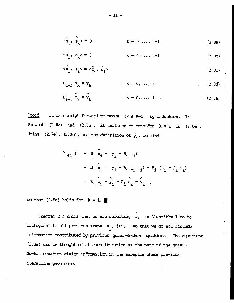
Sk>= 0 k = 0,..., i-i (2.8a)
<S., S> = 0 k = 0,..., i-i (2.8b)
A A A<s., S.> = <s,, s.> (2.8c)1 1 1 1
B÷1 Sk = (2.9d) -
B.1 Sk = k = 0,. ., i . (2. 8e)
Proof It is straightforward to prove (2.8 a-d) by induction. In
view of (2.8a) and (2.7e), it suffices to consider k = i in (2.8e).
Using (2. 7e), (2. 8c), and the definition of we find
A A
B. S. = B. S. + (y - B. s.)i+l 1 3. 1 j 1 1
= B. S. + (y. - B. Q. s.) - B. (s. - 0. s.)3. 1 1 1 1 1 1 1 1 1
A A A A= B. S. + y. - B. s. = y.11 1 11 1
so that (2. 8e) holds for k = i.
Tira 2.2 shows that we are selecting s in Algorithm I to be
ort1gonaj. to all previous steps s, j<i, so that we do not disturb
information contributed by previous quasi-Newton equations. The equations
(2.8e) can be thought of at each iteration as the partof the quasi-
Newton equation giving information in the subspace where previous
iterations gave none.

— 12 —
Note that if B. and B1 are nonsinguJ.ar, then (2.7e) is equivalent to
(s. — B.1 y) T B.1B.1 = B. + 1 1 1 1 ]. (2.9)11 1 AT —1s B y
Therefore if B is nonsingular and <sj, B1 y>0 for 0 < j < i, then
B1 exists, i.e., B+i iS flOflSinU.lr.
We now state, in general form, the version of our new algorithm
which is used in practice and in proving local Q-superliflear conver-
gence. it recognizes that, in general1 the projection of s orthocJO1l
to the subspace spanned by So,... ,s1im.ist be the zero vector for sane
i < n. The algorit1Et therefore "restarts" by setting s = s if
is too small canpared to Si (which rrn.ist happen at least every n steps).
ThecrEn 2.2 is still valid if we consider only the vectors s, ' 'generated since the last restart. Since the version of TheorEn 2.2
applicable to Algorithm ii is needed in Section 4, it is stated as
TheorEn 2.3. The anitted proof is a1irst identical to that of TheorEn 2.2.
Because of the restart iteria, s is alcays strongly linearly indepen-
dent of all s 's since the last restart.
Algorithm II
Let X0 £, B0F c > 0, 't > 1 be given.
Set
For i = 0, 1, 2,...Choose nonzero s (likely s = —X B1 F (xi))

—13—
x1 = x. + s.(2.lOa)
If I J< C then stop
y. = F(x.1) — F(x.) (2.lOb)
i—i S. S.Q. = E (2.lOc)
J=. S. Si—i j j
1± IIs.II > -r s. — Q. s.J (2.i')d)1 — 1 11then (s = S1 arid = i)
else (. = S. — Q. S. and 9... =
,rr(y. — B. s.) s.
B.1 = B. + 1 1 1(2.lOe)
Theorn 2.3 Given x C IR, B0 c F C > 0, -r > 1, let the
sequences {s,... ,s1}, Cy,. . . ,y.}, {B,. . . ''÷l be generated by Algorithm
II. Define {, .. . ,} as in Algorithm II; let = y if s= s and
y. = y. - 13. Q. s otherwise, j = 0,. . . ,i. Then at each iteration i,
s , ... ,s are linearly independent, B1 is well defined, and1
<s., = 0 k = L,...,i—1 (2.lla)
<s., Sk> = 0 k = 2..,.. . ,i—l (2.llb)

— 14 —
A A A
<s., s.> = <s., s.> (2.llc)1 1 1 1
B1 Sk= k = Zr,.. j (2. lid)
B.1 5k =ic = 2.... ,i (2. lie)
IIsII < ilisHi (2.lif)
(2.llg)
We finally note that the entire subject of quasi - Newton methods for
nonlinear systans of equations can be approached by directly fozning
approxitnations H to F' (xi) -1, the inverse of the Jacobian matrix of F at x.
In this case we require H1 y = s and can achieve this through the
rark -one update
T(s. - H. y.) w.= H + 1 1 1 1 (2.12)
w. y.1 1
for any vector w. c such that y o. we have already seen
fran (2.9) that if B. is non-singular, Broyden' s update sitriply corresponds
-rtow1
= B. s in (2.12).
The choice of w in (2.1Z which mi.nimizes the Frobenius norm of
(H+i - H.) is w = The quasi-Newton method using this update was
also proposed by Broyden and is saTetimes called "Broyden' s bad rrethxl",
because it doesn't perform as well as Broyden's method (update (2.4)) in

— 15 —
practice. However, it has also been dconstrat1 by Broyden, Dennis, and
Ibr [1973 to have local superlinear convergence under reasonable assurrtions
on F.
Similarly, we can propose a1gorit1ns I' and II', which update
approximations H1 to F' (x1) , arid choose w in (2.12) to be the
projection of y. orthogonal to (sorr of) the previous y 's. For
instance, Algorithm II' would only require replacing (2. lOc—e) with
i—I= E 'j Y (2.13a)1
j=9.i—i y y
IfI II I > TI — Q4' yI I
then (y. y and 9.. = i) (2.13b)
else (y. = y — Q.' y and =
H. = H. + (s. - H. y (2.13c)i+l 1. 1 11 1yi Y
Using Algorithms I' or II' we can prove theorems analagous to 2.2 and 2.3;
and we can prove the sane convergence results for linear and general
nonlinear functions F as are proven in Sections 3 and 4. (As a matter of
fact, the proofs of Section 3 are then a bit nicer as they never need
asse B11 non-singular). We have tested hoth algorithms II and II'

—16—
In practice, and have fotrid that AlgoritlTn II appears irore likely to
nverge than II'.

—17—
3. Behavior on Linear or Partly Linear Problems
In this section we examine the behavior of our algorithm on
systems of n equations in n unknowns, some or all of which
are linear. We find that our algorithm will always locate a
zero of whichever of the equations are linear in n+l or fewer
iterations. This property is not shared by Broyden's method.
Theorems 3.1 and 3.2 examine the behavior of Algorithm I on
a corp1etely linear system. In reality we woulc not expect to
use our algorithm to solve linear equations. However, it is
possible that near a solution, a system of nonlinear equations
may be almost linear--and these theorens then tell us what sort
of behavior to expect.
Theorem 3.1 shows that if Algorithm I is applied to
F(x) = Ax + b, A nonsingular, then x will equal x = -Ab for some
i < n+l; and if ri+1 iterations are required, then B = A. Follow-
ing Powell [1976),however, we are really more interested in
Theorem 3.2, which shows what happens if we do a restart wiile
solving a linear system of equations. This is likely to be the
case if we enter a linear region after the algorithm starts.
Theorem 3.2 shows that we still require at most n+2 iterations
to firu , but Example 3.3 shows that B+l may not equal A.
Theorems 3.4 and 3.5 examine the behavior of Algorithm I
when some but not necessarily all of the component functions of
F are linear. This may be the most important case in section
3, as partly linear systems do arise in practice; they may also
approximate the behavior of a nonlinear system near a solution.
—18—
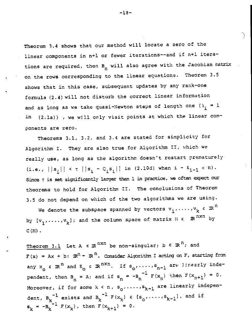
Theorem 3.4 shows that our method will locate a zero of the
linear components in n+l or fewer iterations—-and if n+l itera-
tions are required, then B will also agree with the Jacobian rratrix
on the rows corresponding to the linear equations. Theorem 3.5
shows that in this case, subsequent updates by any rank-one
formula (2.4) will not disturb the correct linear information
and as long as we take quasi-Newton steps of length one (X1= 1
in (2.la)) , we will only visit points at which the linear coin-
ponents are zero.
Theorems 3.1, 3.2, and 3.4 are stated for simplicity for
Algorithm I. They are also true for Algorithm II, ihich we
really use, as long as the algorithm doesn't restart prematurely
(i.e., IIjI < Hs — Q.s.H in (2.lOcl) when i — 9i—1 <
Since T is set significantly larger than 1 in practice, we often expect our
theorems to hold for Algorithm II. The conclusions of Theorem
3.5 do not depend on which of the two algorithms we are using.
We denote the subspace spanned by vectors V1 ,V
by (v1 ,vk]; and the column space of matrix M by
C(M).
Theorem 3.1 Let A flXfl be non-singular; b C and
F (x) = Ax + b: - ]R. Consider Algorithm I acting on F, starting from
any x C and E C If s0 ,s_1 are ]irearly inde-
pendent, then B = A; and if Sn = -B1 F(x) then F(Xn+i)= 0.
Moreover, if for some k < n, s ISk_1 are linearly indepen-
dent, Bk1 exists and k1 F(xk) c [slSk_lI1 arid if
Bk1 F(xk), then F(xk+l) = 0.

—19—
Proof.: If s,... ,s1 are linearly independent, then by Theorem
2.2, Ens. = y, i = O,...,n—l. Since y = F(x.1) — F(x.) = ASi,
we have B S. = A s., i = O,...,n—l, so that B = A.fll 1 fl
If 5'••'5k1 are linearly independent, then by the same
reasoning as above,B.s. = A s., i = O,...,k-l. Thus if11 1
Sk = 3k F(xk) [s...,skl], then Bk 5k = A Sk . Therefore
F(xk÷l) = F(xk) + A Sk = F(xk) + Bk Sk = F(x) + Bk [_Bk1 F(xk)] 0.
IFrom the proof of Theorem 3.1, we see that if ALjorithni II i
acting on a linear problem, then after n—rn iterations in which
s,.. .,s1 are linearly independent and no restarts have occurred,
Em will agree with A in n-rn directions-—i.e., (A -Bn_rn) will
have rank in. It is possible——especially if we have entered a
linear region after we began--that we will then do a restart:
set = s and 2. = n—rn. Following Powell [1976], wen-rn n—rn n-rn
wonder if the information from these n—rn iterations is of help.
In Theorem 3.2 we show that. it is: using quasi-Newton steps (1.3a),
we require at most m+2 additional iterations, or a total of n+2, to
locate the zero of F. Our conclusions are not as general as
Powell's for Davidon's [1975] new unconstrained optimization
algorithm, as they do not allow for subsequent restarts or com-
pletely general steps; however, our conditions should mirror the
behavior of Algorithm II in practice. Also, in our case Example
3.3 shows that the full m+2 iterations may be required and thatBm+i
may still not equal A.

Proof: We first show that for any update of form (2.4)-—one of
which is used by Algorithlr. I-— that s e Es0for some
j < m + 1. We accomplish this by showing by induction that if
'. ,s_1 are linearly independent, then
Si C [s0,CCI - BQ1A)1
(3.1)
(s — B1y)c C (I — BQ1A) • (3.2)
For i = 0, (3.1) is trivi.1ly true, and
— Bol y0 = S0- B01 A S0 = (I -
BQ1A) s0 C C(I -BQ1A).
Assume (3.1-2) true for i = 0,... ,k. Then1 —l 1
-Xk+l
Sk+l — 3k+l F(xk+l) = Bk+l (F(xk) +
By Theorem 2.2, B,,+l1Yk=
$3,;and using the inverse form of (2.4) have
-1 T -1
-l — B1 +
(Sk - Bk 'k Vk BkBk+l
— k T -1Vk Bk
—20—
Theorem 3.2 Let A , b c , and F(x) = Ax + b: +
Consider Algorithm I taited from x0 C and B0 C nxn
singular with rank (A - B0)= n > i. suppose s. is selected by
Si = —X. B.1 F(x) and if s. ' (s0,...,S_i]r assume B1 is
nonsingular.Then there exists j < in + 1 such that
Si C (s01...1s_1);and if X = 1, then F(x±1) = 0.
<Vkl Bk1 F(xk)>
Bk+11 F(xk) = 3k F(x1j + - Bk1 -l<Vkl Bk k>

—21—
Since Bk F(xk) = -Ski we have E [Ski (sk - Bk' k'
so by the induction hypothesis (3.1-2) for k,Sk+l c [5, C(I - E1A)J, which shows (3.1) for i = k+1. To corn-
plete the induction, Sk+l - Bk+,yk+ =
I -1 T —1I - k (s.-B. y.)v. B.= s —'B +k+1 °
j0 T -1 ,L 3 J 3
k <v., B. >— -1 -l -—Sk÷l
-B0 k+1 + E0 (Si -
<vj, B.
Since Sk+l - B01 'k+1 = (I - B1A) Sk+l and
(s - C C (I-B0A) for j < k by the induction
hypothesis, we see that (3.2) holds for i = k+1.
Because the subspace [s0, C (I - B01A)] has dimension at
most m+1, we must have S. C Is01.. .s1] for some j < m+l. NowB. = i = 0,...j-3. by Theorem 2.2; and B s1 = A s, i = 0,
,j—l since F is linear. Therefore B S. = A s, and
F(x.1) = F(x.) + A S. = F(xi) + B. (_B' F(x.)] = 0. 1
Example 3.3. Let F(x) x . (F'(x) I). Consider
Algorithm I, with s = -B1 F(x.) started from x0 = (1and
10 011.
oB = : •iio...o
1...10....01L)rn n-rn
—22—
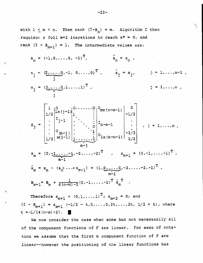
with 1 < m < n. Then ran] (I-B0) = m. Algorithm I then
requires full jn+2 iterations to reach x = 0, and
rank (I - B1) = 1. The intermediate values are:
Ts0 = (—1,0,.. .10, —1) , s =
S0
Si o, ,0)T , s. = s., j = l,...,m—1
x = 11)'P , j = i,... ,r
10 0 00 0
lx(j—l). mx(n—m—l)
1/2 1 : —1/2
'j-•l .• . IB
= . . .. n—rn—i . , = im•
. '•l(n—j ) . 01/2 x(j1) i lx(n—m—1) 1/2'—v_S---1
Sm= (0,,•••,_1,21•,2)T = (01_1,•••,_1)T
=Sm
—
(so+...+srn...i)= (1101•••,01_2,••,_2,_1)T
Bl= B + 4(nm)20'1'••• ,-1)
Therefore S+i = (011)T; X+2 = 0; and
(I —Bm+i)
= S+i (—1/2 — t,0,...,0,2t,...,2t, 1/2 + t), where
t =-1/(4(n—m)-2). •We now consider the case when some but not necessarily all
of the component functions of F are linear. For ease of nota-tion we assume that the first in component function of F are
linear--however the positioning of tb€ linear functions has

—23--
no bearing on the algorithm or the proof. The Jacobian of F
will therefore be constant in its first m rows, and we will de-c.
note our Jacobian approdn'ations B by [ ) , C c
D. R(nm)xn1
Theorem 3.4 Let A c mxn 1 < m < n; b
EF (x)lF(x)=
F2(x)j
Consider Algorithm I acting on F, starting from any and
B e . If for some k < n, s01... FSk_l are linearly ince-
pendent, Bk' exists and Bk1 F(xk) c [soI...lskl], then the
choice Sk = 3k F(xk) leads to F1 (xk÷1) = 0. Furthermore if
s,... ,s1 are linearly independent, then C = A.
Proof: Suppose s,... ,5ki are linearly independent and Bk1
exists. By Theorem 2.2, Bk s = y, 0 < i < k-i. Since the
first m components of y are F1(x÷1) — F1(x) = A s, while the
first m components of Bk s equal Ck s, we have Ck s1 A s,o < i < k-i. In particular, if k = n then this irrplies C = A. More-
over, if Bk F(Yk) [s,... ,sk_1] (which will necessarily hold
for some k < n) and Sk = F (Xk)l then this implies
Ck Sk = A Sk; because Ck Bk1 = (I 0mx(n-m)' we thus have
Fl(xk+l) = Fl(xk) + A Sk = Fl(xk) -Ck Bk1 F(xk)
=Fl(xk)
-Fl(xk) = 0
—24—
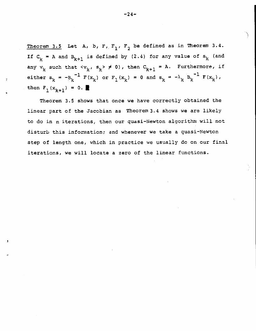
Theorem 3.5 Let A, b, F, F1, F2 be defined as in Theorem 34.
If Ck = A and Bk+l is defined by (2.4) for any value of Sk (and
any Vk such that <Vkl Sk> 0), then Ck+l = A. Furthermore, if
either Sk = Bk F(xk) or Fl(xk) = 0 and Sk Ak Bk1 F(xk),
then Fl(xk+l) = 0. I
Theorem 3.5 shows that once we have correctly obtained •the
linear part of the Jacobian as Theorem 3.4 shows we are likely
to do in n iterations, then our quasi-Newton algorithm will not
disturb this information; and whenever we take a quasi-Newton
step of length one, which in practice we usually do on our final
iterations, we will locate a zero of the linear functions.

—25—
4. Local Q—Superlinear Convergence on Nonlinear Problems
In this section we show, subject to reasonable conditions
on the function F : ]R" - :iRrl, that if x is close enough to x
and if is close enough in norm to F' (x*) [or F' (x0)], then
the sequence of xi's generated by Algorithm II with s = —B11F(x)converges Q—superlinearly to x. Our proof leans heavily
on the local superlinear convergence proof of Broyden, Dennis,
and More [1973] for Broyden's method; and On the work of Dennis
and Nor& [1974] characterizing superlinear convergence.
In Theorem 4.2, we give a general condition under which a
quasi-Newton algorithm of form (2.1) with steplength one will
achieve linear convergence. This theorem amounts to Theorem 3.2
in Broyden, Dennis, Mor [1973] extended to updates using infor-
mation from previous iterations. Lemmas 4.3 and 4.4 show that
the update of gorithm II satisfies the conditions of Theorem
4.2 along with some further conditions. Using this we show in
Theorem 4.5 that Algorithm II achieves local Q-superlinear con-
vergence. We first state a simple lemma which we will use
several times; its proof follows immediately from §3.2.5 of
[Ortega & Rheinboldt, 1970].
Lemma 4.1 Let F: rI + be ciifferertialle in the open convex
set D, and suppose for some x* c D and p > 0, 1< > 0 that
F'(x) - FI(x*)II < K Ix - x*HP (4.1)
Then foru, veD,
IF(v) - F(u) - F' (x*) (v-u)
< KI Iv—uI Imax { v_x*I Iu_x*I P} • (4.2)

—26—
Theorem 4.2 Let F : - be differentiable in the open
convex set D, and assume for some x c D and P > 0, K > 0 that
(4.1) holds, where F(x*) = 0 and F' (x*) is nonsingular. Let
J = F'(x*). Consider sequences Cx0, x11...} of points in
and {, '••• of nonsingular matrices which satisfy
Xk+l_XkkF(Xk)and
'1k+l — IIF . Hk HF + c max flIXk+l -
I x* I1. .., (4.4)
lIXk — x*It°}
k = 0,1,..., for some fixed > 0 and q > 0, '1ere x. = x for— — J 0
j < 0. Then for each r c (0,1), there are positive constants
e(r), d(r) such that if x0 — x*II < (r) and lIE0 — JHF < 5(r),then the sequence x,x1,...} is well-defined and converges to x
with
I jX - x*l I < ri Xk- x*l
I
for all k > 0. Furthermore, {I IBkI } and Cj tkt are uni-
forinly bounded.
The proof is so similar to that of Theorem 3.2 of (Broyden,
Dennis, & Mor, 1973] that we omit it. I
In Lemma 4.3 we show that for Sj y. defined in Algorithm II,
asymptotically I Iy — F' (x*) sJ I is small relative to I IsI
This is the key to proving in Lemma 4.4 that the update of Algor-
ithni II satisfies equation (4.4) of Theorem 4.2.
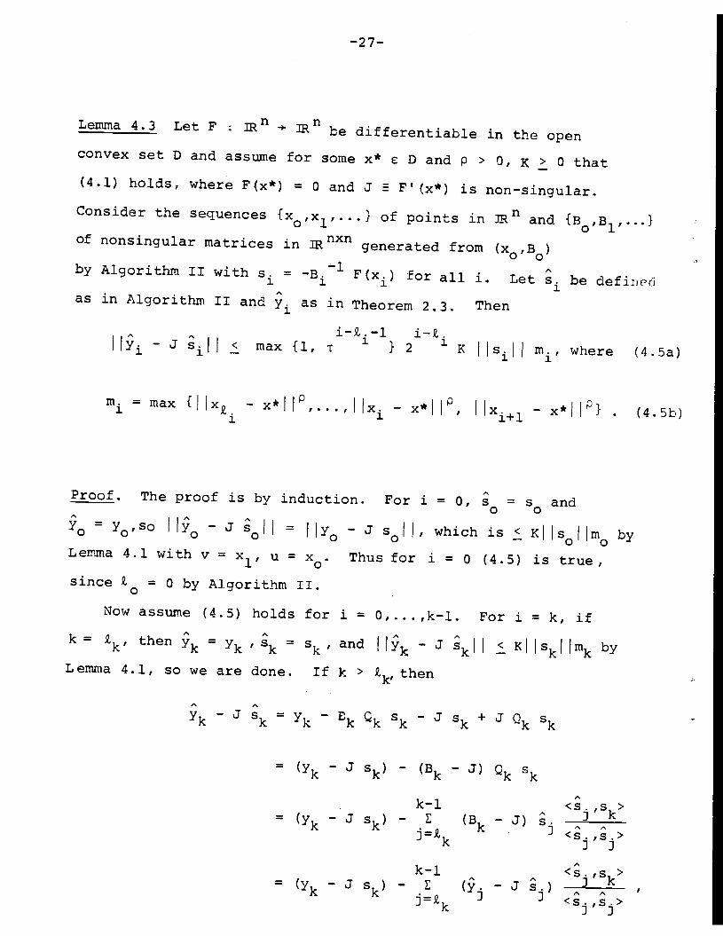
Lemma 4.3 Let F IRn be differentiable in the open
convex set D and assume for some x c D and p > 0, K > 0 that
(4.1) holds, where F(x*) = 0 and J E F' (x*) is non-singular.
Consider the sequences {x ,x11. . .} of points in JR' and {B,B11...}
of nonsingular matrices in )R generated from (x0,B)—l Aby Algoritjt II with S. = -B. F(x.) for all i. Let S. be defined
as in Algorithm II and y. as in Theorem 2.3. Then
i—Z..—l i—iili
— j < max {1, T1
} 2
Proof. The proof is by induction. For i = 0, =S0 and
= 0,so - J J I = j y - J sI J, which is < KJ sf fIn byLemma 4.1 with v = x1, u = x. Thus for i = 0 (4.5) is true,
Since = 0 by Algorithm II.
Now assume (4.5) holds for i = 0,... ,k-i. For i = k, if
k = £k, then 'k = ' S =Ski and 'k
-Ski J < KI
ISki Ink by
Lemma 4.1, so we are done. If k > 'k' then
= - JS})
-(Bk
- j) k Sk
k—i <s.,s >A j k(YkJsk) E (Bk_J)s. AJ<sj,sj>
k—i <.,s >= (y — J s ) — E (. —A Ak k J <s. s.>-, k j'j
—27—
1<I
s m , where (4.5a)i i
max {f Jx — x*f ,..., lxi — x*J l, I Ix÷1 — *f P} (4.5b)I
YkJSk_YkEkksk_Jsk+ Sk

—28—
the last equation following from 3k s = in Theorem 2.3.
Therefore
I
— S]j — J S1 +
j-Lk— Li Sj11 IlSklI/ISII.
Thususing Lemma 4.1, induction hypothesis 4.5, (2.llf), and the
fact that m., 1= the definition of we have
1k - J ii S)J Xflk + KJ Ski i9
h—i j—2. —l j—L s.+ E T 2 K is Hrn
''sillk-i
}
K ISki Imk{1 + 1 + E (2T)k
- k—i< K rr., TkLkl 1 + E 29'k}
=kt mk 1k-2.k-l 2 k-2.k
which proves (4.5) for i = k and comp1tes the induction. I
Lemma 4.4 Let all the conditions of Lemma 4.3 hold. Then
I IB÷ — J. < JB. —'F
/1 — ®.2 + (2t)1 K rn.1
(4.6a)
where- J)
o = 1 1 (4.6b)1 - II H.ll1 F 1

—29--
Proof: Using the definitions of s and y along with the equa-
tion <s., S.> = <i., •> from Theorem 2.3, we find1 i 1 1
(y. - B. s.)T
1 1 1ATS.
1
(. - B.=E. + 1 1 1 -
1 S. S.1 1
ATS.
1
There fore -S. S. I
1 ii— J) —A T A +S. S.'
-- 1 iJ
A AT— J s.) s.1 1
AT AS. S.1 1
BrOyden, Dennis,
U C I
and Mor nxn(1973] show that for E C m and
i—..—l<max {l, T 1
22 HEuH= lIEu - ____
2F Hul
B. =B.+1+1 1 S.1
B. -J1+1
= (B.1
I lB+1 — , 'F
(9
(B. - J)— 1
A A TS. S.1 — 1 1ATA
I S. S.1 1
and
- J S.)1TAS. S.1 1+v±
ATS.1
F
(4.7)
Thus- uuHE r T1— u uJ F
A AT2. 1J)
E
s. S.
H2- AT AS. S. P
2. 1
A A A Til(y. — J s.) S. H1 1 1 II
HS. S. ii
1 1 F
Secondly
(B - J)A 2
lB. - JI1
= -
= IIj — J lIAS.
1
F
(4. 8a)
(4.8b)
Ils.!I 1iF ——— 2
I II
n-im. < (2T) Km.1—
from (2.11 f—g) and Lemma 4,3. Combining (4.7—8) gives (4.6). I
Lemma 4.4 shows that Algorithm II satisfies the conditions
of Theorem 4.2 and is locally linearly convergent for any
r (0 1). The extra power supp1i by the /1 - term in equa-
tion (4.6) enables us to prove local Q-superlinear convergence.
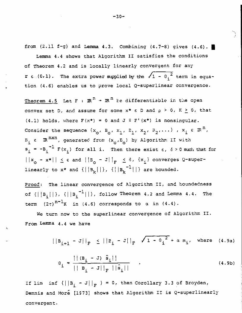
Theorem 4.5 Let F : - e differentiable in the open
convex set D, and assume for some x c D and p > 0, K > 0, that
(4.1) holds, where F(x*) = 0 and J F' (x*) is nonsingular.
Consider the sequence {x0, B0, x1, E,, x2, 2' • I E
flXfl, generatec fron (x0,E0) by Algorithm II with
s1 = -B. F(x.) for all i. Then there exist , >0 such that for
— < and -'F < S, {x} converges Q-super
linearly to x and CiIBJ }, C k1' are bounded.
Proof: The linear convergence of Algorithm II, and houndedness
of CIIB.II}, {lIBII}1 follow Theorem 4.2 and Lemma 4.4. The
term (2T)'K in (4.6) corresponds to a in (4.4).
We turn now to the superlinear convergence of Algorithm II.
From Lemma 4.4 we have
IIB1 — JHF . — /i- G.2 + a m1 where (4.9a)
— J)e. = . (4.9b)1 H B. - JIIF Ilsill
If lirn inf { -'F
= 0, then Corollary 3.3 of Broyden,
Dennis and More [lS73] shows that Algorithm II is Q-superlinearly
convergent.
—31—
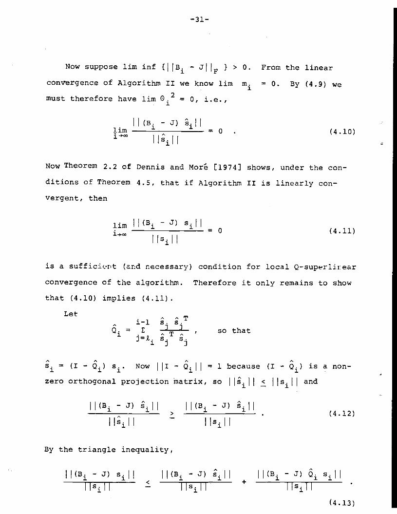
Now suppose urn inf { lB1 - i 'F> 0. From the linear
convergence of Algorithm II we know urn m1 = 0. By (4.9) we
must therefore have lim = 0, i.e.,
(B. - J) s•urn 1 = 0 . (4.10)
lklJ
Now Theorem 2.2 of Dennis and More [1974] shows, under the con-
ditions of Theorem 4.5, that if Algorithm II is linearly con-
vergent, then
ll(B. — J)urn 1 1 = 0 (4.11)
I lsI I
is a sufficicr't (and necessary) condition for local Q—superlirear
convergence of the algorithm. Therefore it only remains to show
that (4.10) implies (4.11).
Leti-l
Q. = E 2T , so that1 j=i. S. S.13 J
S1= (I - Q) s. Now 1 - = 1 because (I - Q) is a non-
zero orthogonal projection matrix, so I IsH and
- J) II(B. - J)1 1 1 1 (4.12)IiII
-11s4 H
By the triangle inequality,
II (B — J) SjI (B — J)+
I (B — J) Q sIISjIJ
— IlSjlI IISjII
(4.13)

—32—
As i+, the first term on the right hand side of (4.13) approa-
ches zero due to (4.10), (4.12). For the second term on the
right side of (4.13), Theorem 2.3 and Lemma 4.3 show
i—i
I (B — J) Sj1 =I
— J) s>/< >I I
j=zi
i—i= 1Z ( — J ) <i., s.>/<, >I I
i-i j-.-1 j-i. IIs.IIrnax{1,t
1 }2 1K— IIH• Is. rn.
1 J
Because IsII/IIII < T (by (2.llf)) and rn < rn.1, jZ,...,i—1
with i-2.. < n (by (2.ilg)), we thus have
i—2.—1 i—i j—..
H (B — 3) sj I . KI Isj rnj.1 T1
21
i—Z.—1 i—i..
5. XI IsI T1
21
rnj....1
n—2 n—i< iI s. 2 m.— 1 i—i
Hence
I! (s sdj < K n—2 2n—i rn1 , so
lint I I (B — j) I = n , (4.14)HH

-33—
since im m. = 0. Therefore (4.10) and (4.12—14) imply (4.11)1
is true, which completes the proof of local Q—superlinear con-
vergence of Algorithm II.
It should be noted that the techniques of this section apply
equally well to an algorithm identical to II except restarting
whenever i — R..l > t, t < n (or I Is.I I/I lsI I > T). Such an
algorithm would not be exact on linear problems, however. Ano-
ther interesting algorithm covered by the techniques of this
section is one setting
<S. , S.>i—i 1S. = 5. — S.1 1 i—l<s. ,s. >i1 i—l
at each iteration. Such an algorithm would preserve the current
and most recent quasi—Newton equation at each step, and can be
shown by the techniques of this section to be Q-superlinearly
convergent without restarts. We have not tested this algorithm.
Finally, the techniques of this section would also apply to
an algorithm which set s ecual to the projection of s ortho-
gonal to the previous t si's, t <n,suhject to the strong linear
independence of . . ,s. as in Algorithm II. Such an algorithm
would require no restarts arid would be exact for linear problems
if b = n. It would be fairly easy to implement (in 0(n2) house-
keeping operations per step) using Powell's [1968] orthogonaliza-
tion scheme.

—34—
5. Computational Results
We have implemented Algorithms II and II', with some modifica-
tions,and tested them on several problems. In Step (2.lOa) we
choose s = -.X B.1 F(x.), where ). is determined by the scheme
described in rBroyden, 1965] with the added restriction that
I Isj I < 1 (except as otherwise noted). Instead of storing
we actually store and update H = 3l• Rather than compute Q
explicitly by frmu1a (2.lOc), we use ajpropriate Householder
transformations to express in product form an orthogonal matrix
P such that
= p , whence s — =
L n—i+2._1
Our implementation includes the option suggested above of restart.xszj
whenever i-L. >t, where t < n is fixed. For t = 1 this lets us--
try Broyden's original methods on the test problems.
Test Problems
The test problems we used include the following; we write x1
th 1 Tfor the i— component of x = (x ,. .. ,x ) c
Prob1 3. [Frown, 1969, p. 567]: n = 5.
nf. (x) = —(n+l) + 2x1 + x, 1 < i < n—i1 j=1
jin
f (x) = —1 + 11 Xn
j=l
T T= (.5 5) ; * (1 11)

—35.-
Problem 2 [Brown, 1969, p. 567] : n = 2.
i2 2(x) —x —1.
1 2 2 2= (x —2) + (x — .5) — 1
x0 = (.1,2); x (1.06735, 139228)T
Problem 3 - "Chebyqd' - [Fletcher, l965,y. 36] : n = 2,3,4,5,6,7,9.
1 inf(x) = / T()d - E T(xJ), where T. is the Chebyshev
0 j=11
polynomial, transformed to the interval [0,1], i.e. T0() 1,
T1() = 2 — 1, T1() = 2(2—1)T() — T.1() for i > 1. Note
that
110 if i isodd
/ T. ()d =1 l-l/(i2-l) if is is even.
x = j/(n+l), 1 < j < n; the components of a solution are any
permutation of the abscissae for the Chebyshev quadrature rule of
order n.
None of the variations of Broyden's method which we tried
solved this problem for r=9, so we omit the results of these runs.
Problem 4 (Brown and Conte, 19671: n = 2
2 11 12 x x
f1(x) = sin (x x ) - - --
f2(x) = (1 — ) [exp(2x1) — e] + — 2ex1
x0= (63)T. x = (5)T

—36—
Problem 5 (Erown arid Gearhart, 1971, p. 341): n = 3.
12 22f1(x) = (x ) + 2(x )
— 4
12 22 3
f2(x) = (x ) + (x ) + x - 8
f3(x) = (x11) + (2x2 - + (x-5)2 - 4.
= (1, .7, = (0, /• 6)T
Problem 6 [Deist and Sefor, l962j_ ri = 6
6
f(x)= E cot $.x, 1 < i < 6, where
j=1 1
j1
1'• '6 = io2 (2.249, 2.166, 2.083, 2, 1.918, 1.833)
x0 = (75, 75,• ,75); x (121.850, 114.161, 93.6483,
62.3186, 41.3219, 30•5027)T
Problem 7 [Broyden, 1965) n = 5, 10.
(.5x—3)x1 + 2x2 — 1.
f(x)= + (.5x1—3)x1 + 2xj1 — 1, 2 < n—i
f(x)= xr1 + (.5x-3)x - 1.
Tx0
= (—1, —i,...,—1)
For n = 5, x* (—. 968354, —1.18696, —1.14848, —.958989, _594159)T
and for n = 10, x (1.0301l, —1.31044, —1.37992, —1.39071,
-1.37963, -1.34993, -1.29066, -1.17748,—.975O1. 5657)T

—37—
We ran our tests in double precision on the IBM 370/168 at
Cornell University. Table I below gives the results of some of
these tests. 1'Probiern ct. means probiemc with n =
For each test problem we report both the actual nuriber of
function evaluations needed to achieve IFI < 1010 and a
normalized number of function evaluations obtained by dividing
the actual number by the minimum of the three numbers for that
problem (and rounding to two decimal places). Although Algorithm
II sometimes fares worse then Broyden's good method, the means
of the normalized numbers show that Algorithm II with T = 10
averaged about 10% fewer function. evaluations than Broyden's
good method on these test. prc1lems. The choice T = 10 worked
considerably better than T = 100 in Algorithm II, suggesting
that a reasonably small value of T, such as 10, may be best.
We ran several other tests, whici we shall not report in
detail. True to its name, for example, Broyden's bad method
failed six times as often as his good method. Algorithm II'
with -r = 10 failed on 5 of the 15 test runs; with T = 100 it
failed on only 3, but fared rather worse than Broyden's good
method with respect to mean normalized function evaluations.
We tried a hybrid between Algorithms II and II' whose average
behavior for T = 10 was as good as that of Algorithm II. The
hybrid applies the projections of Algorithm II' to the inverse
form of Broyden's good method, so that y - is replaced by
T A A T(I - Q)H. S. and the choice = y is replaced by y = H Si.

Total FunctionEvaluations
FunctionEvaluationsRequired toAchieveI
< 1010
—38—
Normalized FunctionEvaluations
Algorithm II__________ T = 10 T = 100
Notes: 1. Eroyden's [1965] quadratic interpolation techniquefailed to reduce IFI i in 10 function evaluations.The number reported is the total number of functionevaluations at the time of failure.
2. I IFI was allowed to incr3ase as much as twofold(per step) and a maximum steplength of 10 ratherthan 1 was allowed.
3. A maximum steplength sj of 10 rather than 1was allowed.
P robl emBroyden' S'hhi Algorithm II
r=lO T1003royden' S"Good"
1.5 31 27 28 1.15 1.00 1.04
ii.
3.2 9
3.3 13
10 ltD 1.10 1.00 1.00
9
11
23
9
13
1.00
1.18
1.00
1.00
1.00
1.18
19 23 1.00 1.21 1.21
3.5
3.6
3.7
20 24
(31)1 26
45 35
23
33
—
36—
1.00 1.20
-- 1.00
1.29 1.00
1.15
1.27
1.03,4.2 12 10 10 1.20 1.00 1.005.3
532
15
16 15
(28)1(28)1
15
1.00
1.07
-- --1.00 1.00
6.6 62 29 60 2.14-
1.00 2.07
6.62 32 28—
57
—1.14 1.00 2.04
7.5 13 13 13 1.00 1.00 1.00
7.10 21 20 20 1.05 1.00 1.00
Table I: Mean 1.17 1.03 1.21
Std.Dev .29 .074 .37
Failures 1 1 1,

—39—
6. Summary and Conclusions
We have introduced some new quasi-Newton algorithms for
solving systems of n non-linear equations in n unknowns. These
methods are modifications of 'Broyden's good method" and "Broy—
den's bad method' (Broyden [1965]). They retain the local Q—
superlinear convergence of the unmodified methods and have the
additional property that if any of the equations are linear,
then the methods locate a zero of these equations in n+1 or
fewer iterations. (We have only proven these properties in this
paper for the modified Broyden's good method, but virtually the
same proofs go through for the modified bad method.)
Our computational results suggest that our modified form of
Broyden's good method performs better, on the average, than the
original form. We think our new method should be further tested
and possibly considered as a replacement for the conventional
Broyden's method in existing subroutines.
Acknowledgement
We are grateful to Professor 14.J.D. Powell for helpful discus-
sions and advice.

—40—
7. References
Brown, K.I4. (1969), "A Quadratically Convergent Newton-LikeMethod Based Upon Gaussian Elimination," SIAM J. Numer.Anal. 6, pp. 560—569.
Brown, 1CM., & Conte, S.D. (1967), "The Solution of SimultaneousNonlinear Equations," Proc. 22nd National Conference of theACM, Thompson nook Co., Washington, D.C., pp. 111-114.
Brown, I.N., & Gearhart, W.B. (1971), "Deflation Techniques forthe Calculation of Further Solutions of a Nonlinear ystcm,"Nurer. Math. 16, pp. 334—342.
Broyden, C.G. (1965), "A Class of Methods for Solving NonlinearSimultaneous Equations," Math. Comput. 19, pp. 577-593.
Broyden, C.G.; Dennis, J.E.; & Mor, J.J. (1973), "On the Localand Superlinear Convergence of Quasi-Newton Methods," J.Inst. Math. Appi. 12, pp. 223—245.
Davidop, tT.C. (1975), "Optimally Conditioned Optimization Algor-ithins cithout Line Searches," Math. PrograInxruiii 9, pp. 1-30.
Deist, F.H.; & Sefor, L. (1967), 'Solution of Systems of Non-linear Equations by Parameter Variation," Comput. J. 10,pp. 78—82.
Dennis, J.E., Jr.; & More, J.J. (1974), "A Characterization ofSuperljnear Convergence and Its Application to Quasi-NewtonMethods," Math. Comput. 28, pp. 549-560.
Dennis, J.E., Jr.; & More, J.J. (1977), "Quasi-Newton Methods,Motivation and Theory," SIAM Rev. 19, pp. 46-89.
Fletcher, R. (1965), "Function Minimization Without EvaluatingDerivatives; a Review," Comput. J. 8, pp. 33-41.
Garca-palomar U.M. (1973), "Superlinearly Convergent Quasi-Newton Methods for Nonlinear Programming," Ph.D. disserta-tion, University of t'7isconsjn.
Gay, D.M. (1977), "Convergence Properties of Eroyden-rype Methodson Linear Systems of Equations," in preparation.
Ortega, J.M.; & Rhejnbcldt, W.C. (1970), Iterative Solution ofNonlinear Equations in Several Variables, Academic Press,New York.

—41—
Powell, M.J.D. (1968), "On the Calculation of Orthogonal Vectors,"Comput. J. 11, PP. 302-304.
Powell, M.J.D. (1976), "Quadratic Termination Properties ofDavidon's New Variable Metric Algorithm," Math. Programn-iing,(to appear).
Schnabel, R.B. (1977), Ph.D. Thesis, Computer Science Dept.,Cornell University.
Related Documents