Particle Swarm Optimization for Solving Nonlinear Programming Problems A PROJECT PAPER SUBMITTED IN PARTIAL FULFILLMENT OF THE REQUIREMENTS FOR THE DEGREE OF MASTER OF SCIENCE IN MATHEMATICS SUBMITED TO NATIONAL INSTITUTE OF TECHNOLOGY ROURKELA BY Rakesh Moharana Roll Number: 413MA2063 UNDER THE GUIDANCE OF Dr. Santanu Saha Ray DEPARTMENT OF MATHEMATICS NATIONAL INSTITUTE OF TECHNOLOGY ROURKELA Rourkela - 769008 May, 2015

Welcome message from author
This document is posted to help you gain knowledge. Please leave a comment to let me know what you think about it! Share it to your friends and learn new things together.
Transcript

Particle Swarm Optimization for SolvingNonlinear Programming Problems
A PROJECT PAPER SUBMITTED IN PARTIAL FULFILLMENT OF THE
REQUIREMENTS FOR THE DEGREE OF
MASTER OF SCIENCE
IN
MATHEMATICS
SUBMITED TO
NATIONAL INSTITUTE OF TECHNOLOGY ROURKELA
BY
Rakesh Moharana
Roll Number: 413MA2063
UNDER THE GUIDANCE OF
Dr. Santanu Saha Ray
DEPARTMENT OF MATHEMATICSNATIONAL INSTITUTE OF TECHNOLOGY ROURKELA
Rourkela - 769008May, 2015

Declaration
I hereby certify that the work which is being presented in the report entitled “Particle Swarm
Optimization for Solving Nonlinear Programming Problems ” in partial fulfillment of the
requirement for the award of the degree of Master of Science, submitted to the Department
of Mathematics, National Institute of Technology Rourkela is a review work carried out
under the supervision of Dr. Santanu Saha Ray. The matter embodied in this report has
not been submitted by me for the award of any other degree.
(Rakesh Moharana)
Roll No-413MA2063

iii
NATIONAL INSTITUTE OF TECHNOLOGY ROURKELA
ROURKELA, ODISHA
CERTIFICATE
This is to certify that the thesis entitled “Particle Swarm Optimization for Solving
Nonlinear Programming Problems ” submitted by Rakesh Moharana (Roll No:
413MA2063.) in partial fulfilment of the requirements for the degree of Master of Science
in Mathematics at the National Institute of Technology Rourkela is an authentic work carried
out by him during 2nd year Project under my supervision and guidance.
Date: 11th May, 2015Dr. Santanu Saha Ray
Associate ProfessorDepartment of Mathematics
NIT Rourkela
iv
Abstract
In the beginning we provide a brief introduction to the basic concepts of optimization and
global optimization, evolutionary computation and swarm intelligence. The necessity of
solving optimization problems is outlined and various types of optimization problems are
discussed. A rough classification of established optimization algorithms is provided, followed
by Particle Swarm Optimization (PSO) and different types of PSO. Change in velocity com-
ponent using velocity clamping techniques by bisection method and golden search method
are discussed. We have discussed advantages of Using Self-Accelerated Smart Particle Swarm
Optimization (SAS-PSO) technique which was introduced . Finally, the numerical values of
the objective function are calculated which are optimal solution for the problem. The SAS-
PSO and Standard Particle Swarm Optimization technique is compared as a result SAS-PSO
does not require any additional parameter like acceleration co-efficient and inertia-weight as
in case of other standard PSO algorithms.

ACKNOWLEDGEMENT
This work would not have been possible without the support and encouragement of the fol-
lowing persons, and I wish to extend my deepest gratitude to each of them. I would specially
like to express my deep sense of gratitude and respect to my supervisor Dr. Santanu Saha
Ray for his excellent guidance, suggestions and constructive criticism. I consider myself
extremely lucky to be able to work under the guidance of such a dynamic personality.
I would like to render heartiest thanks to our Ph.D. Research Scholars who’s ever helping
nature and suggestion has helped me to complete this present work.
Last but not least I would like to thank my parents and specially my brother Rajesh
Moharana for his support.
Date: 11th May, 2015Rakesh Moharana
M.Sc 2nd yearRoll.No.- 413MA2063
Department of MathematicsNIT Rourkela
v

Contents
1 Introduction 1
1.1 Optimization . . . . . . . . . . . . . . . . . . . . . . . . . . . . . . . . . . . 1
1.2 Types of optimization problem . . . . . . . . . . . . . . . . . . . . . . . . . . 2
1.3 Classification of optimization algorithms . . . . . . . . . . . . . . . . . . . . 4
2 Particle Swarm Optimization (PSO) 6
2.1 Source of inspiration . . . . . . . . . . . . . . . . . . . . . . . . . . . . . . . 6
2.2 Early Variant of PSO . . . . . . . . . . . . . . . . . . . . . . . . . . . . . . . 7
2.3 Swarm explosion and velocity clamping . . . . . . . . . . . . . . . . . . . . . 10
2.4 Concept of Inertia weight . . . . . . . . . . . . . . . . . . . . . . . . . . . . . 11
3 PSO Algorithms 13
3.1 Standard particle swarm optimization (SPSO) . . . . . . . . . . . . . . . . . 13
3.1.1 Individual best algorithm . . . . . . . . . . . . . . . . . . . . . . . . 13
3.1.2 Global Best Algorithm . . . . . . . . . . . . . . . . . . . . . . . . . . 14
3.1.3 Velocity component and coefficients . . . . . . . . . . . . . . . . . . . 15
3.2 PSO using constraint fitness priority-based ranking method . . . . . . . . . . 20
3.3 Self-Accelerated Smart Particle Swarm Optimization for multi-modal Opti-
mization Problems (SAS-PSO) . . . . . . . . . . . . . . . . . . . . . . . . . . 22
4 Conclusion 24
Bibliography 25
vi
Chapter 1
Introduction
In this chapter, we provide brief introductions to the basic concepts of optimization. The
necessity of solving optimization problems is outlined and types of optimization problems
are discussed. A rough classification of optimization algorithms is provided.
1.1 Optimization
The term optimization is a scientific discipline which deals with the finding of an optimal
solution for a given problem among all the alternatives. This optimality of solutions is based
on one or many criteria and conditions which are problem-dependent and user-dependent.
So in many problems constraints are posed by the user or given in problem itself, to reducing
it in to the number of prospective solution. So from here onwards the term feasible solution
arises which states that, if the solution satisfies all constraints then it is a feasible solution.
So from all the feasible solution global optimization problem deals with the identification
of the optimal one. Sometimes it may not be possible also. In some cases where subopti-
mal solutions are acceptable, depending on their value compared with the optimal one and
it is known as local optimization. A modeling phase is always precedes the optimization
procedure. The real problems are modeled mathematically, taking all the constraints in
to account. Finally, proper mathematical functions are built. These functions are called
1
2
objective functions. The objective function accompanied by domain, i.e., a set of feasible
candidate solution. The problem is delimited by problem constraints, which need to be
described mathematically by using equality and inequality relation. Analytical derivation
of solutions is possible for some problems. Indeed, if the objective function is atleast twice
continuously differentiable and has a relatively simple form, then its minimizers are attained
by determining the zeros of its gradient and verifying that its Hessian matrix is positive
definite at these points. Apparently, this is not possible for functions of high complexity
and dimensionality or functions that do not fulfill the required mathematical assumptions.
In the latter case, the use of algorithms that approximate the actual solution is inevitable.
Such algorithms work iteratively, producing a sequence of search points that has at least one
subsequence converging to the actual minimize.
Optimization has been an active research field for several decades. The scientific and techno-
logical blossoming of the late years has offered a plethora of difficult optimization problems
that triggered the development of more efficient algorithms. Real-world optimization suffers
from the following problems (see [10]).
a) Problem in detecting global optimal solution from local optimal solutions.
b) The “curse of dimensionality”, i.e., exponential growth of the search space with the prob-
lem’s dimension.
c) Difficulties associated with the problem’s constraints.
1.2 Types of optimization problem
Optimization problems or minimization problems can be defined mathematically in many
ways, depending on the following applications. Generally any function f : X → Y defined
over a domainX also is a search space having range Y . So in literature, common optimization
problems consisting minimization of function, whose domain is a subset of Rn(Euclidean

3
space) and the range is a subset of R. And the problem may have constraints in the form
of inequality relations. So the minimization problem can be written formally
minx∈X
f(x), Subject to Mj(x) ≤ 0; j = 1, 2, . . . , k
where X ⊆ Rn and Y ⊆ R is subset of the n−dimension Euclidean and real numbers
Different types of optimization:
i) Linear optimization (or linear programming): It studies cases where the objective func-
tion and constraints are linear.
ii) Nonlinear optimization (or nonlinear programming): It deals with cases where at least
one nonlinear function is involved in the optimization problem.
iii) Convex optimization: It studies problems with convex objective functions and convex
feasible sets.
iv) Quadratic optimization (or quadratic programming): It involves the minimization of
quadratic objective functions and linear constraints.
v) Stochastic optimization: It refers to minimization in the presence of randomness,
which is introduced either as noise in function evaluations or as probabilistic selection of
problem variables and parameters, based on statistical distributions.
Usually, optimization problems are modeled with a single objective function, which remains
unchanged through time. However, many significant engineering problems are modeled with
one or a set of static or time-varying objective functions that need to be optimized simulta-
neously. These cases give rise to the following important optimization subfields:
a) Dynamic optimization: It refers to the minimization of time-varying objective func-
tions (it should not be confused with dynamic programming). The goal in this case is to
track the position of the global minimizer as soon as it moves in the search space. Also, it
aims at providing robust solutions, i.e., solutions that will not require heavy computational
costs for refinement in case of a slight change in the objective function.

4
b) Multi-objective optimization: It refers to problems where two or more objective func-
tions need to be minimized concurrently. In this case optimality of solutions is redefined,
since global minima of different objective functions are rarely achieved at the same minimiz-
ers.
A different categorization can be considered with respect to the nature of the search space
and problem variables:
a) Discrete optimization: In such problems, the variables of the objective function assume
discrete values. The special case of integer variables is referred to as integer optimization.
b) Continuous optimization: All variables of the objective function assume real values.
c) Mixed integer optimization: Both integer and real variables appear in the objective
function.
1.3 Classification of optimization algorithms
Generally there is two major type of optimization algorithms that are well known; one is
deterministic and another is stochastic algorithms. Although stochastic elements may ap-
pear in deterministic approaches to improve their performance, this rough categorization
has been adopted by several authors, perhaps due to the similar inherent properties of the
algorithms in each category (Archetti and Schoen, 1984; Dixon and Szego, 1978). Deter-
ministic approaches are characterized by the exact reproducibility of the steps taken by the
algorithm, in the same problem and initial conditions. On the other hand, stochastic ap-
proaches produce samples of prospective solutions in the search space iteratively. Therefore,
it is almost impossible to reproduce exactly the same sequence of samples in two distinct ex-
periments, even in the same initial conditions. Deterministic approaches include grid search,
covering methods, and trajectory-based methods. Grid search does not exploit information
5
of previous optimization steps, but rather assesses the quality of points lying on a grid over
the search space. Obviously, the grid density plays a crucial role on the final output of the
algorithm. On the other hand, trajectory-based methods employ search points that traverse
trajectories, which (hopefully) intersect the vicinity of the global minimizer. Finally, covering
methods aim at the detection and exclusion of parts of the search space that do not contain
the global minimizer. All the aforementioned approaches have well-studied theoretical back-
grounds, since their operation is based on strong mathematical assumptions (Horst and Tuy,
2003; Torn and ilinskas, 1989). Stochastic methods include random search, clustering, and
methods based on probabilistic models of the objective function. Most of these approaches
produce implicit or explicit estimation models for the position of the global minimizer, which
are iteratively refined through sampling, using information collected in previous steps. They
can be applied even in cases where strong mathematical properties of the objective function
and search space are absent, albeit at the cost of higher computational time and limited
theoretical derivations and a more refined classification of global optimization.

Chapter 2
Particle Swarm Optimization (PSO)
2.1 Source of inspiration
Bird flocks, fish schools, and animal herds constitute representative examples of natural
systems where aggregated behaviours are met, producing impressive, collision-free, and syn-
chronized moves. In such systems, the behavior of each group member is based on simple
inherent responses, although their outcome is rather complex from a macroscopic point of
view. For example, the flight of a bird flock can be simulated with relative accuracy by
simply maintaining a target distance between each bird and its immediate neighbours. This
distance may depend on its size and desirable behavior. For instance, fish retain a greater
mutual distance when swimming carefree, while they concentrate in very dense groups in
the presence of predators. The groups can also react to external threats by rapidly changing
their form, breaking in smaller parts and re-uniting, demonstrating a remarkable ability to
respond collectively to external stimuli in order to preserve personal integrity. Common
properties are:
a) Proximity: Ability to perform space and time computations.
b) Quality: Ability to respond to environmental quality factors.
c) Diverse response: Ability to produce a plurality of different responses.
d) Stability: Ability to retain robust behaviors under mild environmental change.
6

7
e) Adaptability: Ability to change behavior when it is dictated by external factors.
2.2 Early Variant of PSO
Particle Swarm Optimization is an algorithm capable of optimizing a non-linear and multi-
dimensional problem which usually reaches good solutions. The algorithm and its concept of
“Particle Swarm Optimization”(PSO) were introduced by James Kennedy and Russel Eber-
hart in 1995. The idea of swarm intelligence based off the observation of swarming habits
by certain kinds of animals (such as birds and fish). The basic concept of the algorithm is
to create a swarm of particles which move in the space around them (the problem space)
searching for their goal, the place which best suits their needs given by a fitness function. A
nature analogy with birds is the following: a bird flock flies in its environment looking for
the best place to rest (the best place can be a combination of characteristics like space for
all the flock, food access, water access or any other relevant characteristic).
Putting it in a mathematical framework, let X ⊆ Rn be the search space and f : X → Y ⊆ R
be the objective function. PSO is a population-based algorithm, i.e., it exploits a population
of potential solutions to probe the search space concurrently. The population is called the
swarm and its individuals are called the particles; a notation retained by nomenclature used
for similar models in social sciences and particle physics. The swarm is defined as a set

8
S = {x1, x2, . . . , xN} of N particles defined as:
xi = (xi1, xi2, . . . , xin)T ∈ X, i = 1, 2, . . . , N
The objective function, f(x) is assumed to be available for all points in X. Thus, each
particle has a unique function value, fi = f(xi) ∈ Y. The particles are assumed to move
within the search space, X iteratively. This is possible by adjusting their position using a
proper position shift, called velocity, and denoted as:
vi = (vi1, vi2, . . . , vin)T , i = 1, 2, . . . , N
Velocity is also adapted iteratively to render particles capable of potentially visiting any
region of A. If t denotes the iteration counter, then the current position of the i− th particle
and its velocity will be denoted as xi(t) and vi(t) respectively.
Velocity is updated based on information obtained in previous steps of the algorithm. This
is implemented in terms of a memory, where each particle can store the best position it
has ever visited during its search. For this purpose, besides the swarm, S, which contains
the current positions of the particles, PSO maintains also a memory set P = p1, p2, . . . , pN ,
which contains the best positions pi = (pi1, pi2, . . . , pin)T ∈ X, i = 1, 2, . . . , N ever visited by
each particle. These positions are defined as:
pi(t) = argt min fi(t)
Here t stands for iteration. Then PSO approximates the global minimizer with the best
position ever visited by all particles and the global minimizer is denoted with index g of the
best position with the lowest function value in P at a given iteration:
pg(t) = argt min f(pi(t))
Then PSO is defined by the following:
vij(t+ 1) = vij(t) + c1R1(pij(t)− xij(t)) + c2R2(pgj(t)− xij(t)) (2.2.1)

9
xij(t+ 1) = xij(t) + vij(t+ 1) (2.2.2)
where i = 1, 2, . . . , N and j = 1, 2, . . . , n.
Pseudo code for operating of PSO:
Input Number of particles N ; Swarm S; Best position PStep 1. set t← 0Step 2. Initialize S and set P ≡ SStep 3. Evaluate S and PStep 4. While termination criteria not mate.Step 5. Update S using equation (1) and (2)Step 6. Evaluate SStep 7. Update PStep 8. Set t← t+ 1Step 9. End WhileStep 10. Print best position.
At each iteration, after the update and evaluation of particles, best positions are also up-
dated. Then, the new best position of xi at iteration t+ 1 is:
pi (t+ 1) =
{xi (t+ 1) , if f (xi (t+ 1)) ≤ f (pi (t))f (pi (t)) , otherwise
In most optimization applications (See [10]), it is desirable to consider only particles lying
within the search space. So for this situation, bounds are imposed on the position of each
particle, xi to restrict it within the search space, X. If a particle have an undesirable step
out of the search space after the application of equation (2.2.2), it is immediately clamped
at its boundary. In the simple case, the search space can be defined as:
X = [a1, b1]× [a2, b2]× . . .× [an, bn] where ai, bi ∈ R, i = 1, 2, . . . , n (2.2.3)
Condition settings for the particles are:
xij (t+ 1) =
{aj, if xij (t+ 1) < aj,bj, if xij (t+ 1) > bj

10
where i = 1, 2, . . . , N and j = 1, 2, . . . , n.
2.3 Swarm explosion and velocity clamping
The swarm explosion effect was the first issue which arises among all the researchers. It refers
to the uncontrolled increase of magnitude of the velocities, resulting in swarm divergence.
This deficiency is due to the lack of a mechanism for constricting velocities in early PSO
variants, and it was straight forwardly addressed by using strict bounds for velocity clamping
at desirable levels, preventing particles from taking extremely large steps from their current
position.
More specifically, a user-defined maximum velocity bound, vmax > 0 is considered. After
determining the new velocity of each particle with equation (2.2.1), the following restrictions
are applied to the position update with equation (2.2.2):
|vij(t+ 1)| ≤ vmax, i = 1, 2, . . . , Nandj = 1, 2, . . . , n.
If any violation occurs, the corresponding velocity component is set directly to the closest
velocity bound:
vij (t+ 1) =
{vmax, if vij (t+ 1) > vmax
−vmax, if vij (t+ 1) < −vmax
If necessary, different velocity bounds per direction component can be used. The value
of vmax is usually taken as a fraction of the search space size per direction. Thus, if the
search space is defined as in equation (2.2.3), a common maximum velocity for all direction
components can be defined as follows:
vmax =mini{bi − ai}
k

11
Then separate maximum velocity bound per component can be calculated as:
vmax,i =bi − aik
, i = 1, 2, . . . , N.
Velocity clamping by bisection method:
If a search space bounded by the range [−amax, amax] , then the velocity bound is in the range
[−vmax, vmax], where vmax = λ× amax and λ is the user supplied velocity clamping factor in
between 0.1 ≤ λ ≤ 1.0. But in some optimization settings the search space is not centered
on 0 so if the search space [amin, amax], then our velocity bound is vmax = λ × [amax−amin]2
.
Velocity clamping by Golden section search method:
vmax = λ× (√5−1)2
[amax − amin],where 0.1 ≤ λ ≤ 1.0
2.4 Concept of Inertia weight
Although the use of a maximum velocity threshold improved the performance of early PSO
variants, it was not adequate to render the algorithm efficient in complex optimization prob-
lems. Despite the alleviation of swarm explosion, the swarm was not able to concentrate its
particles around the most promising solutions in the last phase of the optimization proce-
dure. Thus, even if a promising region of the search space was roughly detected, no further
refinement was made, with the particles instead oscillating on wide trajectories around their
best positions. The reason for this deficiency was shown to be a disability to control ve-
locities. Refined search in promising regions, i.e., around the best positions, requires strong
attraction of the particles towards them, and small position shifts that prohibit escape from
their close vicinity. This is possible by reducing the perturbations that shift particles away
from best positions; an effect attributed to the previous velocity term in equation (2.2.1).
Therefore, the effect of the previous velocity on the current one shall fade for each particle.
For this purpose, a new parameter, called inertia weight, was introduced in equation (2.2.1),

12
resulting in a new PSO variant
vij(t+ 1) = ωvij(t) + c1R1(pij(t)− xij(t)) + c2R2(pgj(t)− xij(t))
xij(t+ 1) = xij(t) + vij(t+ 1)
where i = 1, 2, . . . , N and j = 1, 2, . . . , n.
The rest of the parameters remain the same as for the early PSO variant of equations (2.2.1)
and (2.2.2). The Inertia weight shall be selected such that the effect of vij(t) fades during
the execution of the algorithm. Thus, a decreasing value of w with time is preferable. A
very common choice is the initialization of ω to a value slightly greater than 1.0 to promote
exploration in early optimization stages, and a linear decrease towards zero to eliminate
oscillatory behaviors in later stages. Usually, a strictly positive lower bound on ω is used to
prevent the previous velocity term from vanishing. In general, a linearly decreasing scheme
for ω can be mathematically described as follows:
ω(t) = ωup − (ωup − ωlow)t
Tmax
t Stands for iteration. And bounds for ω is 0.1 ≤ ω ≤ 1.2.

Chapter 3
PSO Algorithms
3.1 Standard particle swarm optimization (SPSO)
3.1.1 Individual best algorithm
In this PSO algorithm every particle compares its position value with itself only.
Step-1 (Initialization)
First initialize the particle position randomly within the space. At t = 0 the position is xi(0)
of a particle pi ∈ pi(0).Then initialize the particle velocity? vi(0).
Step-2 (Evaluation of particle)
Now evaluate the performance of each particle by using current position Current position is
xi(t) and the fitness value is f(xi(t)).
Step-3 (Comparison)
Now compare the performance of each particles to its best performance thus far
If f(xi(t)) < f(xpbest(t))
a) f(xpbest(t)) = f(xi(t))
b) xpbest(t) = xi(t)
Step-4 (Change the Velocity Vector)
Now change the velocity vector for each particle
vi(t+ 1) = vi(t) + ρ(xpbest(t)− xi(t))
13

14
where ρ is a positive number.
Step-5 (Move to a new position)
Now move each particle to a new position with the new velocity vector.
a) xi(t+ 1) = xi(t) + vi(t+ 1)
b) t← t+ 1
Step-6 Go to step 2 and repeat until convergence.
3.1.2 Global Best Algorithm
(Here every particle compares its current position to the entire swarm best position gbest)
Step-1 (Initialization)
First initialize the particle position randomly within the space. At t = 0 the position is xi(0)
of a particle pi ∈ pi(0).Then initialize the particle velocity vi(0).
Step-2 (Evaluation of particle)
Now evaluate the performance of each particle by using current position.
Current position is xi(t) and the fitness value is f(xi(t)).
Step-3 (Comparison)
Now compare the performance of each particles to its best performance thus far:
If f(xi(t)) < f(xgbest(t)), then
a) f(xgbest(t)) = f(xi(t))
b) xgbest(t) = xi(t)
Step-4 (Change the Velocity Vector)
Now change the velocity vector for each particle
vi(t+ 1) = vi(t) + ρ1(xpbest(t) − xi(t)) + ρ1(xgbest(t) − xi(t))
Step-5 (Move to a new position)
Now move each particle to a new position with the new velocity vector.

15
a) xi(t+ 1) = xi(t) + vi(t+ 1)
b) t← t+ 1
step-6 Go to step 2 and repeat until convergence.
3.1.3 Velocity component and coefficients
where ω,C1, C2 are user supplied coefficients and 0 ≤ ω ≤ 1.2, 0 ≤ C1, C2 ≤≤ 4 and
C1 + C2 ≤ 4. The values r1 and r2 are random in 0 ≤ r1, r2 ≤ 1. ω vi(t) is the inertia
component which responsible to keep the particle moving in the same direction.
(Cognitive component): [C1r1(xpbest(t)− xi(t))]
It act as the particles memory causing it to tend to return the regions of the search space.
In which it has experienced high individual fitness and C1 is the Cognitive coefficient.
(Social component): [C2r2(xgbest(t)− xi(t))]
Causes the particle to move to the best region the swarm has found so far.

16

17
Example:
Let us consider a two dimension function f = 3+x21+x22. We can see that at {0, 0} the value
is minimum. Now initialize particle’s current position, x(t) let it be {x1, x2} = {3.0, 4.0},
and the velocity of particle is v(t) = {−1.0,−1.5}. Now assume that constant w = 0.7,
constant C1 = 1.4, constant C2 = 1.4, and that random numbers r1 and r2 are 0.5 and
0.6 respectively (these are user supplied parameters). Now, let the particle’s best known
position is p(t) = {2.5, 3.6} and the global best known position by any particle in the swarm
is g(t) = {2.3, 3.4}. Then the new velocity and position values are:
V (t+ 1) = ωvi(t) + C1r1 [C1r1(xpbest(t)− xi(t))] + [C2r2(xgbest(t)− xi(t))]
= (0.7× {−1.0,−1.5}) + (1.4× 0.5× {2.5, 3.6} − {3.0, 4.0})
+(1.4× 0.6× {2.3, 3.4} − {3.0, 4.0})
= {−0.70,−1.05}+ {−0.35,−0.28}+ {−0.59,−0.50}
= {−1.64,−1.83}
X(t+ 1) = xi(t) + vi(t+ 1)
= {3.0, 4.0}+ {−1.64,−1.83}
= {1.36, 2.17}

18
Now we observe that the update process has improved the old position {3.0, 4.0} to {1.36, 2.17}.
If we continue the iteration process a more, we can find that the new velocity is the old ve-
locity (times a weight) plus a factor that depends on particle’s best known position, plus
another factor that depends on the best known position from all particles in the swarm.
Therefore, a particle’s new position tends to move toward a better position based on the
particle’s best known position and the best known position of all particles.
Problem:
Function name Mathematical description Range
Schwefel’s function f(x) =n∑
i=1
(−xi) . sin(√|xi|)−500 < xi < 500
Global minimum f(x) = n× 418.9829, xi = −4209687, i = 1, 2, 3, . . . , n.

19
Graph for the global minimum
Fitness values for the problem:
Iterations f(x1, x2)0 416.2455 515.74810 759.40415 793.73220 834.813100 837.9115000 837.965
Optimal 837.965
Problem:
Function name Mathematical description Initialization range
Rosenbrock functiond∑
i=1
(100(xi+1 − xi2)2
)+ (xi − 1)2 [15, 30]d
20
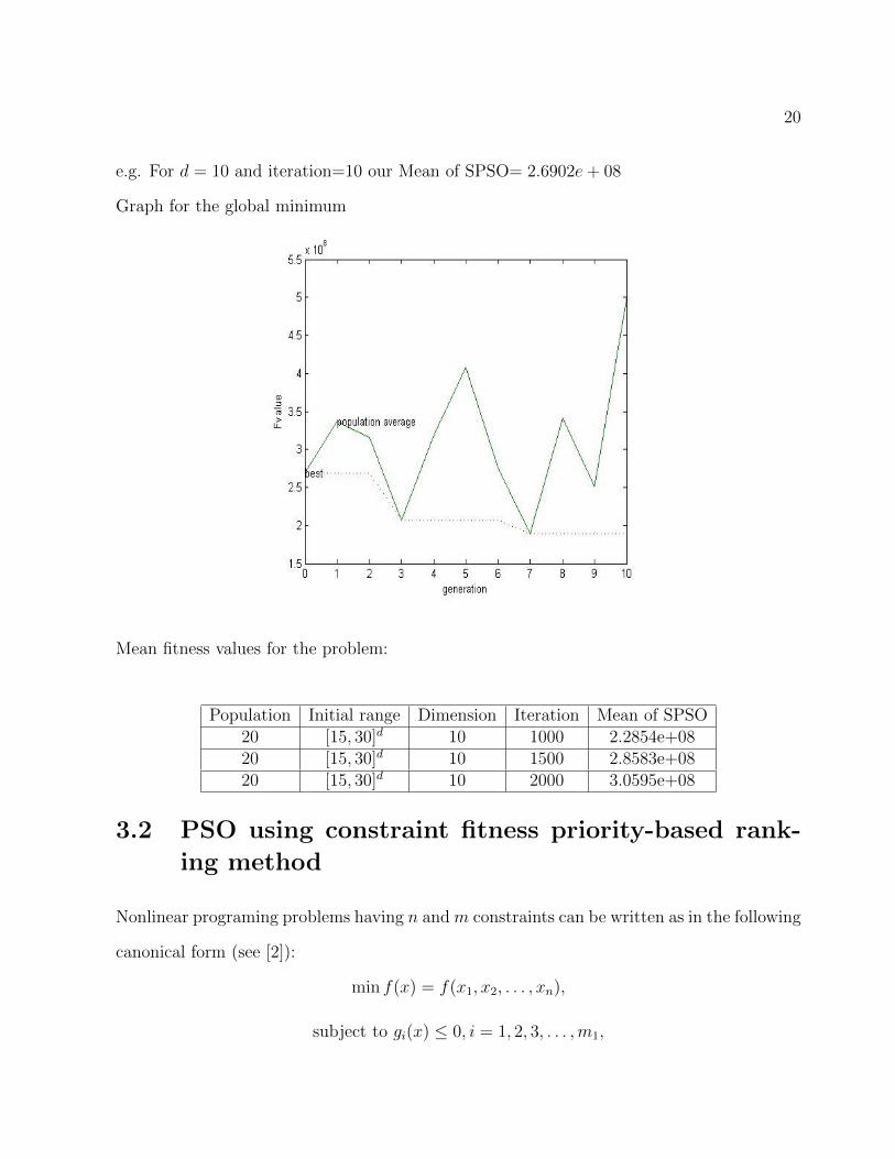
e.g. For d = 10 and iteration=10 our Mean of SPSO= 2.6902e+ 08
Graph for the global minimum
Mean fitness values for the problem:
Population Initial range Dimension Iteration Mean of SPSO20 [15, 30]d 10 1000 2.2854e+0820 [15, 30]d 10 1500 2.8583e+0820 [15, 30]d 10 2000 3.0595e+08
3.2 PSO using constraint fitness priority-based rank-
ing method
Nonlinear programing problems having n and m constraints can be written as in the following
canonical form (see [2]):
min f(x) = f(x1, x2, . . . , xn),
subject to gi(x) ≤ 0, i = 1, 2, 3, . . . ,m1,

21
hi(x) = 0, i = m1 + 1,m1 + 2, . . . ,m.
This method is introduced to solve system constraints.
fobj(x)-optimal fitness function for objective function
fcon(x)- Constraint fitness function
The above function are defined as follows (see [2]):
Definition 1:
fobj(x) = f(x) at x point
Definition 2:
For inequality constraints gi(x) ≤ 0
fi (x) =
{1, gi (x) ≤ 0,
1− gi(x)gmax(x)
, gi (x) > 0
where gmax(x) = max{gi(x), i = 1, 2, . . . ,m1}
For equality constraints hi(x) = 0
fi (x) =
{1, hi (x) ≤ 0,
1− |hi(x)|hmax(x)
, hi (x) 6= 0
where hmax(x) = max{hi(x), i = m1 + 1,m2 + 2, . . . ,m}
Definition 3: fcon(x)-total constraint function at x defined as
fcon (x) =m∑i=1
ωifi (xi),m∑i=1
ωi = 1 , 0 ≤ w1 ≤ 1
Where ωi is the weight for the constraint i.

22
3.3 Self-Accelerated Smart Particle Swarm Optimiza-
tion for multi-modal Optimization Problems (SAS-
PSO)
The SPSO sometimes face a lot problems. So it has some disadvantages like:
1. Sometimes it has bad initialization or local optimal in that case the swarm may converge
prematurely.
2. It requires setting of parameters like C1, C2, ω and λ in velocity clamping
3. When the value of ω increases, as a result it affects the particle which further search for
more global and less local search.
4. When the value of ω decreases, as a result it affects the particle which further search for
less global and more local search.
To overcome from these disadvantages of SPSO, a new version of PSO i.e. SAS-PSO has been
introduced. In SAS-PSO the positions of particles are updated by the following equation
(3.3.1). SAS-PSO doesn’t required any velocity component so it avoids inertia weight and
other coefficients. In this version of PSO momentum factor has used to guide the position
at every iteration (see [1]):
Xi(t+ 1) = Xi(t) +Mc ∗R(Xi(t)− gbest− pbest) + (gbest− pbest) ∗R (3.3.1)
where t= iteration counter, i= Particle Number, Xi(t)= Position of i − thparticle for d−
dimension at iteration t, R= Random values [0, 1] at iteration t, pbest= Personal or local
best of i− th particle at iteration t, gbest = Global best at iteration t and Mc= Momentum
Factor.
Problem:
Function name Mathematical description
Rosenbrock functiond∑
i=1
(100(xi+1 − xi2)2
)+ (xi − 1)2

23
Search and initial range for the problem:
Function Global optima Search range Initial rangeRosenbrock function 0 [−100, 100]d [15, 30]d
Mean fitness value for the problem:
Population Dimension Iteration SAS-PSO20 10 1000 39.845820 20 1500 68.362520 30 2000 79.3246

4. Conclusion
The PSO is an efficient global optimizer for continuous variable problems.it is insensitive
to scaling of design variables, simple implementation, easily parallelized for concurrent pro-
cessing and it is derivative free and can be easily implemented, with very little parameters
to fine-tune. Algorithm modifications improve PSO local search ability. Here we have dis-
cussed SPSO, CPSO, and SAS-PSO which are good. In case of SAS-PSO and SPSO more
efficient is SAS-PSO as we are avoiding velocity component, as we are updating the positon
by its local best and global best. Which helps in optimizing our calculation. In SAS-PSO
other parameters like acceleration coefficient and inertia weight are not required author has
introduced a parameter known as momentum factor Mc which controls particle inside the
search region. This SAS-PSO technique is more efficient to improve the quality of global
optima with less computation.
24
Bibliography
[1] Borkar A. L., “Self-Accelerated Smart Particle Swarm Optimization for multi-modal
Optimization Problems”, Electronics and Telecommunication Dept. M S S S College of
Engineering and Technology Jalna, Maharashtra, India (IJIRSE) International Journal
of Innovative Research in Science and Engineering ISSN (Online), pp. 2347-3207.
[2] Dong Y., Tang J., Xu B. and Wang D.,“An Application of Swarm Optimization to
Nonlinear Programming”, Department of Systems Engineering, Key Laboratory of
Process Industrial Automation of MOE School of Information Science and Engineering,
North-eastern University, Shenyang-110004, P.R. China.
[3] Eberhart R. C., and Shi Y.,“Particle swarm optimization: developments, applications
and resources”, Proc. Congress on Evolutionary Computation, Seoul, Korea, 2001.
[4] Holland J. H., “Adaptation in Natural and Artijlcial Systems”, MIT Press, Cambridge,
1992.
[5] Kennedy J. and Eberhart R., “ Particle Swarm Optimization”, Washington, DC-20212,
Purdue School of Engineering and Technology Indianapolis, IN 46202-5160.
[6] Kennedy J. and Eberhart R.,“Particle swarm optimization”, In Proceedings of the
IEEE International Conference on Neural Networks, volume IV, pages 1942-1948, IEEE
Press, 1995.
25

26
[7] Kennedy J., “Out of the computer, into the world: externalizing the particle swarm.
Proceedings of the Workshop on Particle Swarm Optimization”, Indianapolis,IN: Pur-
due School of Engineering and Technology, IUPUI (in press), 2001.
[8] Kennedy J., Eberhart R. C., and Shi Y, “Swarm Intelligence”, San Francisco: Morgan
Kaufmann Publishers, 2001.
[9] Onwunalu J. and Louis Durlofsky J., “Application of a particle swarm optimization
algorithm for determining optimum well location and type”, 2009.
[10] Parsopoulos K. E. and Vrahatis M. N.,“Particle Swarm Optimization and Intelligence:
Advances and Applications”, Greece.
[11] Shi Y. and Eberhart R., “Experimental study of particle swarm optimization”, Proc.
SCI2000 Conference, Orlando, 2000.
[12] Suganthan P. N., “Particle swarm optimiser with neighbourhood operator”, Proceed-
ings of the 1999 Congress on Evolutionary Computation, pp. 1958-1962, NJ: IEEE
Service Center, 1991.
[13] Zitzler E., Laumanns M., and Bleuler S., “A tutorial on evolutionary multi-objective
optimization”, 2002.
Related Documents