MURRAY-DARLING BASIN COMMISSION ......This summary introduces groundwater modelling concepts and best practice procedures, outlines how groundwater models can be used to help address

MURRAY-DARLING BASIN

COMMISSION

GROUNDWATER FLOW MODELLING GUIDELINE

November 2000

Aquaterra Consulting Pty Ltd ABN 49 082 286 708

_______________________ Hugh MIDDLEMIS 22 Bowman Street Senior Water Resources Engineer South Perth 6151 Western Australia Tel: (08) 9368 4044 Fax: (08) 9368 4055

Project No. 125 Final Guideline – Issue I

16 January 2001

PREFACE

Aquaterra Job# Document Reference Status Issue Date Page 125 F:\jobs\125\B1\Guide\MDBC GW Model Guide-I.doc Final I 28/11/00 P1

Hydrogeological investigations and groundwater modelling are dynamic and inexact sciences. They are

dynamic in the sense that the state of any hydrological system is changing with time, and in the sense that we

are continually developing new scientific techniques to evaluate these systems. They are inexact in the sense

that groundwater systems are complicated beyond our capability to evaluate them comprehensively in detail,

and we invariably do not have sufficient data to do so (even if we had the capability). The ability of the data to

provide an increasingly accurate representation (model) of the groundwater system increases with time,

money, and the technical expertise applied. The study scope and objective needs to be balanced against the

budget, time and data resources available, to develop an appropriate modelling study approach.

This report describes general guidelines for groundwater flow modelling that are designed to reduce the level

of uncertainty for model study clientele, including resource management decision makers and the community,

by promoting transparency in modelling methodologies and encouraging consistency and best practice.

Guidance is provided to non-specialist clientele to outline the steps involved in scoping, managing and

evaluating the results of groundwater modelling studies. Guidance is also provided to modelling specialists to

indicate the technical standards expected to be achieved for a range of modelling project scopes.

The guidelines have been developed for application to groundwater flow modelling projects in the Murray-

Darling Basin, although the approaches are suitable for application to modelling projects generally. The

audience for these guidelines is land and water management planning groups, and resource and technical

staff in government agencies, engineering and hydrogeological consultancies, and the Murray-Darling Basin

Commission.

The guidelines are to be applied to new groundwater flow modelling studies and reviews of existing models.

Solute transport modelling methodologies are not within the scope. The guide should be seen as a best

practice reference point for framing modelling projects, assessing model performance, and providing clients with

the ability to manage contracts and understand the strengths and limitations of models across a wide range of

studies (scopes, objectives, budgets) at various scales in various hydrogeological settings. The intention is not

to provide a prescriptive step-by-step guidance, as the site-specific nature of each modelling study renders this

impossible, but to provide overall guidance and to help make the reader aware of the complexities of models,

and how they may be managed.

Performance indicators are suggested for use in assessing model calibrations in quantitative and qualitative

terms, so that technical and milestone progress can be assessed during modelling projects. Methods for

assessing model uncertainty are also suggested. This methodology also encourages effective communication

and negotiation between modelling specialists and project managers/clientele to achieve project outcomes.

A model review framework is incorporated, with reviews required at all stages throughout the study, consistent

with the objectives, scope, scale and budget of the project. The review is required to be carried out to a level

of detail appropriate for each study, by reviewers with defined capabilities ranging from project manager to

modelling specialists. Checklists are presented for use in model appraisals by non-specialists, and for detailed

model reviews by independent experts.

PREFACE

Aquaterra Job# Document Reference Status Issue Date Page 125 F:\jobs\125\B1\Guide\MDBC GW Model Guide-I.doc Final I 28/11/00 P2

A facilitated workshop was a key component of this project to determine appropriate groundwater modelling

guidelines for application across the Murray-Darling Basin. The workshop was designed to develop consensus

on the content, application and implementation of the draft guidelines by model developers, users and

researchers at federal and state agency, institution and private industry levels. We are grateful for their input,

and for the input of representatives from states outside the Basin, with a view to promulgating these guidelines

across Australia for use in improving modelling study best practice.

The best and most applicable aspects of the published guides and standard text books have been adapted to

develop a guideline that is designed for application to Australian conditions and to resource modelling issues

on a range of project scopes. We acknowledge the authorship of the publications cited.

It is important to note that these guidelines should not be considered as regulation or law, as they have not

received endorsement from any of the jurisdictions they encompass. These guidelines should not be

considered as defacto standards as they are likely to evolve with modelling requirements and the

sophistication of modelling approaches. They also have not been formally endorsed by water managers or

agencies on either a national or Murray Darling Basin basis.

Hugh Middlemis Noel Merrick John Ross Aquaterra University of Technology, Sydney PPK Environment & Infrastructure

TABLE OF CONTENTS

Aquaterra Job# Document Reference Status Issue Date Page 125 F:\jobs\125\B1\Guide\MDBC GW Model Guide-I.doc Final I 28/11/00 i

Summary Section 1 - Introduction.......................................................................................................................................1

1.1 What is a Groundwater Model? ...............................................................................................1 1.2 Need for Guidelines ................................................................................................................2 1.3 Application of the Guidelines....................................................................................................3 1.4 Hydrogeological Framework for the Murray-Darling Basin ......................................................4 1.5 Literature Review ....................................................................................................................4 1.6 Model Complexity.....................................................................................................................6 1.7 Modelling Best Practice............................................................................................................6 1.8 Design of Guidelines................................................................................................................8 1.9 Implementation of Guidelines.................................................................................................10

Section 2 - Conceptualisation ..........................................................................................................................11

2.1 Study Purpose and Model Complexity ...................................................................................11 2.2 Data Collation and Initial Hydrogeological Interpretation .......................................................14 2.3 Consistent Data Units ............................................................................................................17 2.4 Develop Conceptual Model ...................................................................................................18 2.5 Select Modelling Code ..........................................................................................................22 2.6 Model Design, Study Plan, Report and Review .....................................................................25

2.6.1 Model Study Plan......................................................................................................25 2.6.2 Boundary Conditions ................................................................................................26 2.6.3 Model Grids ..............................................................................................................27 2.6.4 Layers .......................................................................................................................28 2.6.5 Profile Models ...........................................................................................................29 2.6.6 Aquifer Units and Parameters...................................................................................29 2.6.7 Water Budget............................................................................................................29 2.6.8 Surface Groundwater Interaction..............................................................................30 2.6.9 Timeframes...............................................................................................................33 2.6.10 Accuracy Targets......................................................................................................34 2.6.11 Resources and Data Required .................................................................................34 2.6.12 Review......................................................................................................................34

Section 3 - Calibration.......................................................................................................................................35

3.1 Construct Model .....................................................................................................................35 3.2 Model Calibration Process .....................................................................................................36

3.2.1 General........................................................................................................................36 3.2.2 Non-uniqueness Problem............................................................................................37 3.2.3 Steady State and Transient Calibration, and Initial Conditions ...................................39 3.2.4 Calibration Acceptance ...............................................................................................41

3.3 Calibration Performance Measures........................................................................................43 3.4 Verify Model as a Predictive Tool...........................................................................................48

Section 4 - Prediction........................................................................................................................................51

Section 5 - Uncertainty Analysis ......................................................................................................................52

5.1 Scoping Uncertainty Assessment ..........................................................................................52 5.2 Sensitivity Analysis.................................................................................................................56 5.3 Uncertainty in Sustainable Yield ............................................................................................56 5.4 Uncertainty in System Stresses .............................................................................................57 5.5 Uncertainty in Aquifer Properties ...........................................................................................60 5.6 Predictive Analysis .................................................................................................................61 5.7 Optimal Groundwater Management .......................................................................................61

TABLE OF CONTENTS

Aquaterra Job# Document Reference Status Issue Date Page 125 F:\jobs\125\B1\Guide\MDBC GW Model Guide-I.doc Final I 28/11/00 ii

Section 6 - Report ..............................................................................................................................................62

6.1 Documentation Types and Model Report...............................................................................62 6.2 Model Archive Documentation ...............................................................................................63

Section 7 - Model Reviews................................................................................................................................67

7.1 Model Appraisal .....................................................................................................................68 7.2 Peer Review...........................................................................................................................68 7.3 Model Audit ............................................................................................................................70 7.4 Post-Audit...............................................................................................................................71

Tables 1.4.1 Murray-Darling Basin Aquifer Systems ....................................................................................................5 1.8.1 Summary of Modelling Methodology........................................................................................................8 2.1.1 Model Study Scope ................................................................................................................................12 2.2.1 Typical Model Data Requirements and Sources....................................................................................15 2.4.1 Conceptual Model Features ...................................................................................................................20 2.5.1 Code Selection Issues ...........................................................................................................................25 2.6.1 Major Types of Model Boundary Conditions ..........................................................................................27 3.2.1 Calibration Acceptability Measures ........................................................................................................41 3.2.2 Pros and cons in relation to prescriptive calibration measures ..............................................................42 3.3.1 Calibration Performance Measures........................................................................................................43 3.3.2 Error listing detailing calibration performance measures .......................................................................47 6.1.1 Model Report Structure and Composition ..............................................................................................64 6.2.1 Example of Model Journal......................................................................................................................66 Figures 1 The groundwater modelling process ........................................................................................................9 2.4.1 Typical cross-section type conceptual model.........................................................................................19 2.4.2 Typical block diagram type conceptual model .......................................................................................20 2.6.1 Surface-groundwater interaction conceptual model...............................................................................32 2.6.2 Evapotranspiration conceptual model ....................................................................................................32 2.6.3 Lake water balance components ...........................................................................................................33 3.2.1 Addressing the non-uniqueness problem...............................................................................................38 3.2.2 Transient calibration and initial conditions .............................................................................................40 3.3.2 Scattergram of measured versus modelled heads.................................................................................46 3.3.3 Calibration contour plot ..........................................................................................................................48 5.2.1 The four types of model sensitivity.........................................................................................................54 5.2.2 Type I Sensitivity ....................................................................................................................................55 5.2.3 Type II Sensitivity...................................................................................................................................55 5.2.4 Type III Sensitivity..................................................................................................................................55 5.2.5 Type IV Sensitivity .................................................................................................................................55 5.2.6 Hypothetical model geometry for excavation dewatering (re Figures 5.2.1 to 5.2.5) .............................56 5.3.1 An example of a cumulative distribution function (cdf)...........................................................................57 5.5.1 Procedure for Monte Carlo Analysis ......................................................................................................59 Appendices Appendix A Literature Review, Annotated Bibliography of Groundwater Flow Modelling Guidelines,

and other References Appendix B Glossary Appendix C Template for a Modelling Study Brief Appendix D Commonly used Numerical Models, and GUIs for Modflow Appendix E Model Appraisal Checklist Appendix F Model Review Checklist Appendix G Checklist for Model Compliance Appendix H Best Practice Modelling Guideline Compilation

SUMMARY

Aquaterra Job# Document Reference Status Issue Date Page 125 F:\jobs\125\B1\Guide\MDBC GW Model Guide-I.doc Final I 28/11/00 S1

INTRODUCTION

This summary introduces groundwater modelling concepts and best practice procedures, outlines how

groundwater models can be used to help address water resources management issues, and provides a

step by step approach to commissioning and understanding groundwater modelling studies.

Groundwater models provide a scientific and predictive tool for determining appropriate solutions to water

allocation, surface water – groundwater interaction, landscape management or impact of new

development scenarios. However if the modelling studies are not well designed from the outset, or the

model doesn’t adequately represent the natural system being modelled, the modelling effort may be

largely wasted, or decisions may be based on flawed model results, and long term adverse consequences

may result. The use of these guidelines will encourage best practice, and help avoid potential problems.

This summary is a “plain English” abstract of the best practice groundwater flow modelling guidelines

prepared for the Murray-Darling Basin Commission (MDBC). This summary has been prepared mainly for

use by community groups, such as catchment management boards, who require groundwater flow

modelling studies to resolve groundwater and catchment management issues. The more comprehensive

technical guideline document contains detailed methodologies and protocols, developed for the MDBC by

the Aquaterra/UTS/PPK project team. The technical document is intended primarily for use by

groundwater management agencies, modellers and auditors of models, rather than the community (which

is the target audience for this summary document).

WHAT IS A GROUNDWATER MODEL?

A groundwater model is a computer-based representation of the essential features of a natural

hydrogeological system that uses the laws of science and mathematics. Its two key components are a

conceptual model and a mathematical model. The conceptual model is an idealised representation (ie. a

picture) of our hydrogeological understanding of the key flow processes of the system. A mathematical

model is a set of equations, which, subject to certain assumptions, quantifies the physical processes

active in the aquifer system(s) being modelled. While the model itself obviously lacks the detailed reality

of the groundwater system, the behaviour of a valid model approximates that of the aquifer(s). A

groundwater model provides a scientific means to draw together the available data into a numerical

characterisation of a groundwater system. The model represents the groundwater system to an adequate

level of detail, and provides a predictive scientific tool to quantify the impacts on the system of specified

hydrological, pumping or irrigation stresses.

Typical model purposes include:

• Improving hydrogeological understanding (synthesis of data);

• Aquifer simulation (evaluation of aquifer behaviour);

• Designing practical solutions to meet specified goals (engineering design);

• Optimising designs for economic efficiency and account for environmental effects (optimisation);

• Evaluating recharge, discharge and aquifer storage processes (water resources assessment);

SUMMARY


• Predicting impacts of alternative hydrological or development scenarios (to assist decision-making);

• Quantifying the sustainable yield (economically and environmentally sound allocation policies);

• Resource management (assessment of alternative policies);

• Sensitivity and uncertainty analysis (to guide data collection and risk-based decision-making);

• Visualisation (to communicate aquifer behaviour).

NEED FOR GUIDELINES

Groundwater investigations, and modelling studies in particular, involve both a science and an art. The

scientific basis is important, and requires a sound knowledge of geology, hydrogeology, groundwater

hydraulics, hydrology, surface-groundwater interaction and engineering, as well as sufficient spatial and

time series data to describe the system. The art is manifest in the creative processes required for

developing a groundwater model as a simple computer-based representation of a complex natural system.

There is also an art in applying experienced judgement where data are lacking to sufficiently rationalise

natural processes, and in effectively communicating the modelling study results.

Best practice modelling is not primarily a question of understanding and implementing the appropriate

mathematical techniques, but of understanding and implementing an appropriate modelling approach.

That is, the approach must be appropriate for the particular site conditions and the stated study objectives.

The clientele (end-users) of model studies (eg. the community or resource managers) generally do not

have (or need to have) this understanding and capability, which is the mark of a competent modeller. In

other words, modellers are specialist service providers to clientele/end-users.

There is a perception amongst end-users of model studies in the Murray-Darling Basin that model

capabilities may have been “over-sold”. There is also a lack of consistency in approaches, communication

and understanding among and between modellers and end-users, which often results in considerable

uncertainty for decision-making. These guidelines are needed to promote best practice modelling

methodologies. They also provide the means by which end-users can plan, initiate and manage modelling

studies, and assess outcomes with reduced uncertainty.

NATURAL RESOURCE PROBLEMS AND MANAGEMENT ISSUES

Most catchment issues that require a greater understanding of groundwater behaviour for evaluating

management options and determining appropriate solutions, relate to either rising or falling water tables.

These fluctuations are commonly related to river regulation, flooding, irrigation development and

associated changes to surface water regimes, groundwater recharge changes due to changing land use,

or groundwater pumping.

Significant changes in catchments across the Murray-Darling Basin, and Australia as a whole, have

occurred in the last hundred years. Many of these changes have been induced by changes in the

hydrology and hydrogeology of catchments, and are today reflected in stressed rivers and groundwater

systems. For groundwater systems, these stresses can either be water level rises or water level declines

SUMMARY


(and associated issues such as water quality impacts) which are impacting the productivity and

environmental sustainability of catchments.

Groundwater models provide a relevant and useful scientific and predictive tool for predicting impacts and

developing management plans. At the workshop to review the draft guidelines, it was clearly

acknowledged that groundwater models should be seen as an integral part of the water resource

management process. This is so because models are increasingly being used to demonstrate the effects

of proposed developments and alternative policies to stakeholders and communities, for the purposes of

gaining consensus on improved allocation distributions and management plans.

WHY DO WE NEED MODELLING STUDIES?

It is not possible to see into the sub-surface, and observe the geological structure and the groundwater

flow processes. The best we can do is to construct bores, use them for pumping and monitoring, and

measure the effects on water levels and other physical aspects of the system. It is for this reason that

groundwater flow models have been, and will continue to be, used to investigate the important features of

groundwater systems, and to predict their behaviour under particular conditions.

Models also form an integral part of decision support systems in the process of managing water

resources, salinity and drainage, and should not be regarded as just an end point in themselves. The

1999 Salinity Audit of the Murray-Darling Basin clearly pointed to the need for a Basin-wide salinity

management strategy that incorporates a revised Salinity and Drainage Strategy. The development and

evaluation of resource management strategies for sustainable water allocation, and for control of land and

water resource degradation, are heavily dependent on groundwater model predictions. Regional scale

groundwater flow modelling studies are commonly used for water resource evaluation and to help quantify

sustainable yields and allocations to end-users.

DETERMINING ROLES and RESPONSIBILITIES

There are many different tasks in building a robust groundwater model. Some of the more important tasks

involve obtaining the very best data set and communicating the results of the study(s). For groundwater

models of all complexities to fully satisfy project objectives, the roles and responsibilities of the project

team must be clearly understood and applied as part of the project management process. In a simple task

breakdown for the development of groundwater flow models for catchment management purposes, the

following roles and responsibilities are suggested:

Community/Clientele

• Define the objectives and model purpose, and outline realistic scenarios for prediction

• Assist with the review of data availability, reliability, location and identify important data gaps

• Review the conceptual model

• Provide information to assist with rationalising data quality problems

• Review the model outputs

SUMMARY


Project Managers/Technical Steering Group

• Specification of the detailed technical brief, including project objectives, model complexity, scope

outline, data availability and quality, budget, timeframe, prediction scenarios, and expected outcomes

and project deliverables

• Determination of model ownership, handover and training requirements, and ongoing model

maintenance plans

• Supply of data sets and relevant technical study reports

• Review and confirmation of conceptual model

• Project and model audit and review at defined milestones

• Acceptance of the final model and report.

Modellers

• Submit model proposal in compliance with brief, clearly stating detailed methodology; key features of

the conceptual model; budget, schedule and team information; and expected deliverables

• Outline the project management structure, major milestones and review plans

• Undertake the literature and technical data review

• Conceptual model development, model code selection, and model study plan

• Model development (calibration, verification, predictions, uncertainty analysis)

• Reporting

• Internal audits and reviews.

THE GROUNDWATER MODELLING TOOL BOX

Groundwater modelling is only one management tool available to catchment managers for developing

solutions to complex catchment issues. Models provide one of the best tools for determining the most

appropriate land/water management options or strategies to adopt. They are rarely the only component of

a large catchment or resource availability study, and are often linked to other socio-economic models and

extensive community consultation initiatives. Modelling can be a very powerful tool when used in the right

circumstances and when models are properly constructed. Accurate and reliable data must be available,

together with a modelling team with proven skills in the local hydrogeology/hydrology and the designated

modelling package. Communication and discussion of modelling results and management implications

between the modelling team, the clientele, and the Technical Steering Group is as important to the

resource management process as specialist modelling skills and tools.

It is strongly recommended that the clientele has a Technical Steering Group (or appropriate

hydrogeological expertise), including an independent groundwater model reviewer, to assist in the

preparation of technical briefs, to provide an inventory of the available data sets, and to review proposals

and reports. Members of the Group should have extensive local knowledge (including hydrogeological

knowledge) and be able to communicate results to all stakeholders.

SUMMARY


DATA REQUIREMENTS

An inventory of available data is required prior to the commissioning of any modelling study. If the

modelling study is being commissioned by a group outside the State agency responsible for catchment /

water management, then the location and accessibility of data held by different agencies should be

determined prior to preparing and releasing the study brief. This data should also be briefly evaluated

prior to preparing any modelling brief to determine its suitability for the management problem and the type

of modelling study required. Typical model data requirements and sources are outlined in the technical

guideline (Section 2).

This data review may redefine the study objectives or initiate data collection networks that are tailored and

specific to the management issue and the required modelling study.

The selected modelling approach should be consistent with the available data sets and the current

conceptual model of the groundwater system. The model should also be flexible enough to be expanded

into a more complex model if more data becomes available and the model is to be used for long term

management of the catchment or aquifer system.

SKILL BASE

The Technical Steering Group must have appropriate hydrogeological skills to help design the model, and

review outcomes of the modelling study. The nominated contractor’s project team must have appropriate

skills to deliver the required modelling study (within the budget and timeframe), support enhancements to

the model, and assist the client in the communication of the model results.

Some of the required skills include:

• knowledge of the local area and the hydrology of the aquifer system

• expertise in the nominated model design and package

• ability to liaise with regulators or agencies to obtain data and to resolve data conflicts and

uncertainties

• being accessible for data acquisition / transfer, meetings and presentations regarding model

development and outcomes

MODEL LIMITATIONS

Limitations and uncertainties exist in any modelling study in regard to our hydrogeological understanding,

the conceptual model design, and model calibration and prediction simulations, as well as recharge and

evapotranspiration estimation and simulation. There are also limitations associated with the capabilities of

the existing groundwater modelling software packages to adequately represent the complexities of any

given hydrogeological system, and particularly in regard to surface-groundwater interaction. These

limitations are best addressed by careful scoping of proposed modelling approaches at the outset (see

next section), and review at various stages throughout the project (see Review section later). It is also

SUMMARY


important that modellers properly document model limitations at the proposal stage and in technical

reports, as well as outlining possible methods of resolving them by subsequent work programmes of data

acquisition and analysis and/or modelling. In some cases, the limitations may be so severe that there may

be little value in putting the effort into a modelling study until more data and hydrogeological

understanding is obtained, or until new technical methods are developed. Consequently the guidelines

recommend that Technical Steering Groups include an independent model reviewer to provide specialist,

unbiased advice to the project team.

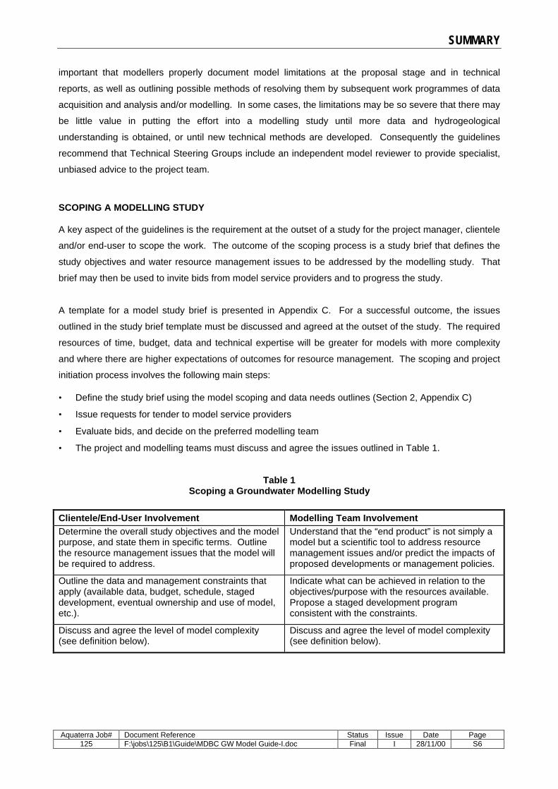
SCOPING A MODELLING STUDY

A key aspect of the guidelines is the requirement at the outset of a study for the project manager, clientele

and/or end-user to scope the work. The outcome of the scoping process is a study brief that defines the

study objectives and water resource management issues to be addressed by the modelling study. That

brief may then be used to invite bids from model service providers and to progress the study.

A template for a model study brief is presented in Appendix C. For a successful outcome, the issues

outlined in the study brief template must be discussed and agreed at the outset of the study. The required

resources of time, budget, data and technical expertise will be greater for models with more complexity

and where there are higher expectations of outcomes for resource management. The scoping and project

initiation process involves the following main steps:

• Define the study brief using the model scoping and data needs outlines (Section 2, Appendix C)

• Issue requests for tender to model service providers

• Evaluate bids, and decide on the preferred modelling team

• The project and modelling teams must discuss and agree the issues outlined in Table 1.

Table 1 Scoping a Groundwater Modelling Study

Clientele/End-User Involvement Modelling Team Involvement Determine the overall study objectives and the model purpose, and state them in specific terms. Outline the resource management issues that the model will be required to address.

Understand that the “end product” is not simply a model but a scientific tool to address resource management issues and/or predict the impacts of proposed developments or management policies.

Outline the data and management constraints that apply (available data, budget, schedule, staged development, eventual ownership and use of model, etc.).

Indicate what can be achieved in relation to the objectives/purpose with the resources available. Propose a staged development program consistent with the constraints.

Discuss and agree the level of model complexity (see definition below).

Discuss and agree the level of model complexity (see definition below).

SUMMARY


Model complexity is defined as the degree to which a model application resembles, or is designed to

resemble, the physical hydrogeological system. There are three main classifications of model complexity

(in order of increasing complexity):

• Basic model - a simple model suitable for preliminary assessment (rough calculations), not requiring

substantial resources to develop, but not suitable for complex conditions or detailed resource

assessment (indicative resources required - $2,000 to $8,000 budget, less than three weeks work)

• Impact Assessment model - a moderate complexity model, requiring more data and a better

understanding of the groundwater system dynamics, and suitable for predicting the impacts of

proposed developments or management policies (indicative resources required - $10,000 to $100,000

budget, one to six months work)

• Aquifer Simulator - a high complexity model, suitable for predicting responses to arbitrary changes in

hydrological conditions, and for developing sustainable resource management policies for aquifer

systems under stress (indicative resources required - more than $50,000 budget and more than six

months work initially – essentially open-ended budgets and long time frames are required for ongoing

development).

To decide on the degree of complexity, and to scope a modelling study, including assessing data

requirements, time and cost, the detailed information in Section 2 and Appendix C provide a useful outline.

In simple terms, model complexity can be described by the “quick-cheap-good” paradox. The end-user

can readily obtain a model with one or two of these three attributes, but not all three. If a model is

required to be done quickly, it can also be done cheaply, but the results may not be good enough on

which to base important resource development or management decisions. Such a simple model may be

good enough for rough calculations to guide a field program, or to assess the broad impacts of a certain

proposal, but would usually not be sufficient for project approval or licensing purposes. Alternatively, if a

good, reliable model is required, then it is not likely to be able to be developed quickly or cheaply.

In less simple terms, the “quick-cheap-good” attributes are better defined in terms of model complexity

(see above). The level of model complexity needs to discussed and agreed between the end-user and the

modeller, to ensure that it suits the study purpose, objectives and resources available for each study. This

involves consideration of the complexities of the hydrogeological system and the design of an appropriate

modelling approach. The data requirements and the level of modelling effort also need to be considered

in relation to the resources available and the overall project objective. Long term requirements may

involve the staged development of a complex model from a simple application (with ongoing data

acquisition and interpretation), and eventual transfer to an end-user as a predictive scientific tool for

resource management.

The model complexity assessment should involve negotiation with the model reviewer as well as between

the end-user and modelling team. In this case, the model reviewer is providing independent expert advice

to model end users to design an appropriate modelling study approach. Government agency

SUMMARY


representatives also should be included in this process (if they are not already part of the project team), as

they will use the model results to allocate water resources and/or to assess the impacts of proposed

developments and/or to implement resource management policies. It is important for the overall project

objectives that potential fatal flaws in the modelling approach are identified and rectified at an early stage,

rather than presenting government agencies with the results of a study that may not be regarded as

scientifically sound.

MODEL DEVELOPMENT

Model development should be undertaken in three main stages, as indicated in Table 2:

Table 2 Summary of Modelling Methodology

Stage Description Tasks

1 Conceptualisation • Define study objectives (general and specific) and model complexity • Complete initial hydrological and hydrogeological interpretation, based on

available data/reports • Prepare conceptual model (in consultative manner) • Select modelling code (analytical/numerical) • Prepare detailed model study plan (outline grid, layers, boundaries, timeframes,

accuracy targets, resources and data required, etc.) • Report and Review • Commonly comprises around 30% (sometimes as high as 60%) of the study

effort 2 Calibration • Construct model by designing grid, setting boundary conditions, assigning

parameters and other data • Calibrate model by adjusting parameters until simulation results closely match

measured data • Complete model verification, and sensitivity and uncertainty analysis • Report and review • Commonly comprises up to 50% of the study effort

3 Prediction • Prediction scenarios • Complete sensitivity and uncertainty analysis • Report and review • Commonly comprises up to 20% of the study effort

After definition of the study objectives, model purpose and complexity at the scoping stage, the most

important step in a modelling study is the development of a valid conceptual model. A conceptual model

is a simplified representation of the key features of the physical system, and its hydrological behaviour. It

forms the basis for the site-specific computer model, but is itself subject to some simplifying assumptions.

The assumptions are required partly because a complete reconstruction of the field system is not feasible,

and partly because there is rarely sufficient data to completely describe the system in full detail.

The conceptual model should be as complex as needs be, but not overly complex for the objectives of the

model. In other words, the model should be kept as simple as possible, while retaining sufficient

complexity to adequately represent the physical elements of the system, and to reproduce hydrological

behaviour. However, the model features must be designed so that it is possible for the model to predict

system responses that range from desired to undesired outcomes. The model must not be configured or

constrained such that it artificially produces a restricted range of prediction outcomes. The model should

SUMMARY


be allowed to evolve (or be refined) with time, as more data is obtained and analysed, and the

understanding of the hydrological and hydrogeological systems is improved.

MODEL PERFORMANCE MEASURES

To assist the project manager, community and/or end-user to assess whether a model has achieved the

level of complexity required, qualitative and quantitative model performance measures are proposed in

these guidelines (summarised in Table 3). Although non-specialists may not readily understand these

technical aspects, they provide relatively simple methods that can be used for contract or milestone

management of modelling studies. Prescriptive performance measures cannot be applied blindly,

however, as model performance can only be gauged against observations which are usually imperfect and

incomplete, and the model must replicate processes which might be poorly understood or inadequately

measured. Model performance measures should be compared to previously agreed target criteria.

Table 3 Model Calibration Performance Measures

Item Performance Measure Criterion

1 Water balance Difference between total inflow and total outflow, including changes in storage, divided by total inflow or outflow, expressed as a percentage.

Less than 1% for each stress period and cumulatively for the entire simulation.

2 Iteration residual error The calculated error term is the maximum change in heads (for any node) between successive iterations of the model.

Iteration convergence criterion should be one to two orders of magnitude smaller than the level of accuracy desired in the model head results. Commonly set in the order of millimetres or centimetres.

3 Qualitative measures Patterns of groundwater flow (based on modelled contour plans of aquifer heads). Patterns of aquifer response to variations in hydrological stresses (hydrographs). Distributions of model aquifer properties adopted to achieve calibration.

Subjective assessment of the goodness of fit between modelled and measured groundwater level contour plans and hydrographs of bore water levels and surface flows. Justification for adopted model aquifer properties in relation to measured ranges of values and associated non-uniqueness issues.

4 Quantitative measures Statistical measures of the differences between modelled and measured head data. Mathematical and graphical comparisons between measured and simulated aquifer heads, and system flow components.

Criteria should be selected from the list of residual head statistics detailed in the technical guideline (Section 3). Consistency between modelled head values (in contour plans and scatter plots) and spot measurements from monitoring bores. Comparison of simulated and measured components of the water budget, notably surface water flows, groundwater abstractions and evapotranspiration estimates.

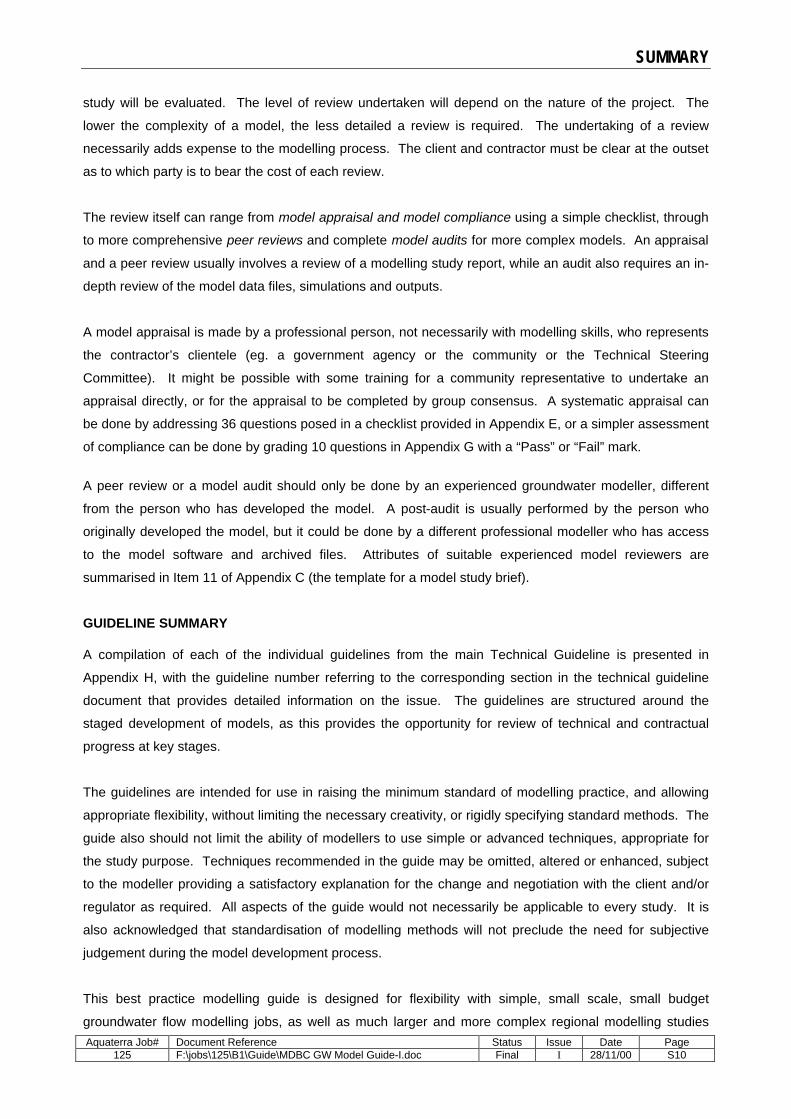
MODEL REVIEWS

A model review framework is another key element of the guideline, with reviews recommended at all

stages throughout the study, consistent with the objectives, scope, scale and budget of the project. A

model review provides a process by which the end-user can check consistently that a model meets the

project objectives. It also provides the model developer with a specification against which the modelling

SUMMARY


study will be evaluated. The level of review undertaken will depend on the nature of the project. The

lower the complexity of a model, the less detailed a review is required. The undertaking of a review

necessarily adds expense to the modelling process. The client and contractor must be clear at the outset

as to which party is to bear the cost of each review.

The review itself can range from model appraisal and model compliance using a simple checklist, through

to more comprehensive peer reviews and complete model audits for more complex models. An appraisal

and a peer review usually involves a review of a modelling study report, while an audit also requires an in-

depth review of the model data files, simulations and outputs.

A model appraisal is made by a professional person, not necessarily with modelling skills, who represents

the contractor’s clientele (eg. a government agency or the community or the Technical Steering

Committee). It might be possible with some training for a community representative to undertake an

appraisal directly, or for the appraisal to be completed by group consensus. A systematic appraisal can

be done by addressing 36 questions posed in a checklist provided in Appendix E, or a simpler assessment

of compliance can be done by grading 10 questions in Appendix G with a “Pass” or “Fail” mark.

A peer review or a model audit should only be done by an experienced groundwater modeller, different

from the person who has developed the model. A post-audit is usually performed by the person who

originally developed the model, but it could be done by a different professional modeller who has access

to the model software and archived files. Attributes of suitable experienced model reviewers are

summarised in Item 11 of Appendix C (the template for a model study brief).

GUIDELINE SUMMARY

A compilation of each of the individual guidelines from the main Technical Guideline is presented in

Appendix H, with the guideline number referring to the corresponding section in the technical guideline

document that provides detailed information on the issue. The guidelines are structured around the

staged development of models, as this provides the opportunity for review of technical and contractual

progress at key stages.

The guidelines are intended for use in raising the minimum standard of modelling practice, and allowing

appropriate flexibility, without limiting the necessary creativity, or rigidly specifying standard methods. The

guide also should not limit the ability of modellers to use simple or advanced techniques, appropriate for

the study purpose. Techniques recommended in the guide may be omitted, altered or enhanced, subject

to the modeller providing a satisfactory explanation for the change and negotiation with the client and/or

regulator as required. All aspects of the guide would not necessarily be applicable to every study. It is

also acknowledged that standardisation of modelling methods will not preclude the need for subjective

judgement during the model development process.

This best practice modelling guide is designed for flexibility with simple, small scale, small budget

groundwater flow modelling jobs, as well as much larger and more complex regional modelling studies

SUMMARY


with substantial resource management implications. The best and most applicable aspects of the

published guides and standard text books have been adapted to develop a guideline that is designed for

application to Australian conditions and to flow modelling issues on a range of project scopes.

The guidelines should have a defined life cycle, and should themselves be reviewed at intervals

(nominally every 5 years), or as technical and project requirements demand. The need for guidelines, or

the type of guideline required, may well be quite different in the future, and may well differ between

agencies/industries and between states.

SECTION 1 - INTRODUCTION

Aquaterra Job# Document Reference Status Issue Date Page 125 F:\jobs\125\B1\Guide\MDBC GW Model Guide-I.doc Final I 28/11/00 1

1.1 WHAT IS A GROUNDWATER MODEL?

Groundwater systems are complicated beyond our capability to evaluate them comprehensively in detail.

Comprehensive analysis means that need to take into account all the characteristics of the system, and

predict the effects of hydrological and land use stresses. There are usually insufficient data to completely

characterise the groundwater system under investigation, and assumptions and simplifications are

required to obtain a quantitative solution for a given problem. We use groundwater models to integrate

our hydrogeological understanding with the available data, to develop a predictive tool for evaluating

groundwater systems, subject to assumptions and limitations.

A groundwater model is a computer-based representation of the essential features of a natural

hydrogeological system that uses the laws of science and mathematics. Its two key components are a

conceptual model and a mathematical model. The conceptual model is an idealised representation

(usually graphical) of our hydrogeological understanding of the essential flow processes of the system. A

mathematical model is a set of equations, which, subject to certain assumptions, quantifies the physical

processes active in the aquifer system(s) being modelled.

While the model itself obviously lacks the detailed reality of the groundwater system, the behaviour of a

valid model approximates that of the aquifer(s). A groundwater model provides a scientific means to

synthesise the available data into a numerical characterisation of a groundwater system. The model

represents the groundwater system to an adequate level of detail, and provides a predictive tool to

quantify the effects on the system of specified hydrological, pumping or irrigation stresses.

In this context, groundwater models provide a relevant and useful scientific tool for predicting impacts and

developing management plans. At the workshop to review the draft guidelines, it was clearly

acknowledged that groundwater models should be seen as an integral part of the water resource

management process. This is a developing area as models are increasingly being used to demonstrate

the effects of proposed developments and alternative policies to stakeholders and communities, for the

purposes of gaining consensus on improved allocation distributions and management plans. This is

regarded as a valuable process, and its continued success depends substantially on the ability of

modelling teams to communicate the results of modelling in terms that are meaningful to the communities

that are affected by the decisions based on the model findings.

Typical model purposes include:

• Improving hydrogeological understanding (synthesis of data); • Aquifer simulation (evaluation of aquifer behaviour); • Designing practical solutions to meet specified goals (engineering design); • Optimising designs for economic efficiency and account for environmental effects (optimisation); • Evaluating recharge, discharge and aquifer storage processes (water resources assessment); • Predicting impacts of alternative hydrological or development scenarios (to assist decision-making); • Quantifying the sustainable yield (economically and environmentally sound allocation policies); • Resource management (assessment of alternative policies); • Sensitivity and uncertainty analysis (to guide data collection and risk-based decision-making); • Visualisation (to communicate aquifer behaviour).

INTRODUCTION


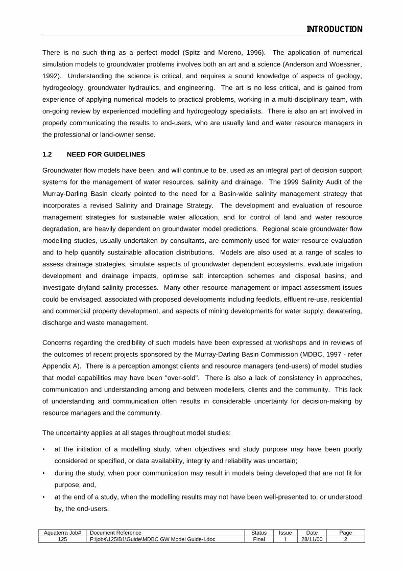
There is no such thing as a perfect model (Spitz and Moreno, 1996). The application of numerical

simulation models to groundwater problems involves both an art and a science (Anderson and Woessner,

1992). Understanding the science is critical, and requires a sound knowledge of aspects of geology,

hydrogeology, groundwater hydraulics, and engineering. The art is no less critical, and is gained from

experience of applying numerical models to practical problems, working in a multi-disciplinary team, with

on-going review by experienced modelling and hydrogeology specialists. There is also an art involved in

properly communicating the results to end-users, who are usually land and water resource managers in

the professional or land-owner sense.

1.2 NEED FOR GUIDELINES

Groundwater flow models have been, and will continue to be, used as an integral part of decision support

systems for the management of water resources, salinity and drainage. The 1999 Salinity Audit of the

Murray-Darling Basin clearly pointed to the need for a Basin-wide salinity management strategy that

incorporates a revised Salinity and Drainage Strategy. The development and evaluation of resource

management strategies for sustainable water allocation, and for control of land and water resource

degradation, are heavily dependent on groundwater model predictions. Regional scale groundwater flow

modelling studies, usually undertaken by consultants, are commonly used for water resource evaluation

and to help quantify sustainable allocation distributions. Models are also used at a range of scales to

assess drainage strategies, simulate aspects of groundwater dependent ecosystems, evaluate irrigation

development and drainage impacts, optimise salt interception schemes and disposal basins, and

investigate dryland salinity processes. Many other resource management or impact assessment issues

could be envisaged, associated with proposed developments including feedlots, effluent re-use, residential

and commercial property development, and aspects of mining developments for water supply, dewatering,

discharge and waste management.

Concerns regarding the credibility of such models have been expressed at workshops and in reviews of

the outcomes of recent projects sponsored by the Murray-Darling Basin Commission (MDBC, 1997 - refer

Appendix A). There is a perception amongst clients and resource managers (end-users) of model studies

that model capabilities may have been "over-sold". There is also a lack of consistency in approaches,

communication and understanding among and between modellers, clients and the community. This lack

of understanding and communication often results in considerable uncertainty for decision-making by

resource managers and the community.

The uncertainty applies at all stages throughout model studies:

• at the initiation of a modelling study, when objectives and study purpose may have been poorly

considered or specified, or data availability, integrity and reliability was uncertain;

• during the study, when poor communication may result in models being developed that are not fit for

purpose; and,

• at the end of a study, when the modelling results may not have been well-presented to, or understood

by, the end-users.

INTRODUCTION


The end-users or model study clientele range from resource managers with professional qualifications and

variable modelling expertise, to community representatives and experienced land managers, usually with

no formal scientific training. The development and implementation of guidelines for groundwater

modelling is designed to reduce the level of uncertainty for decision makers, end-users and the community

by promoting transparency in modelling methodologies, and encouraging consistency, best practice and

greater confidence in the outcomes of the different predictive scenarios. The guidelines are designed for

use by non-professionals, and yet provide professionals with sufficient detail to undertake and manage

modelling studies, and objectively review a model’s fitness for purpose.

1.3 APPLICATION OF THE GUIDELINES

These best practice guidelines are to be applied to new groundwater flow modelling studies and reviews

of existing models. Solute transport and unsaturated zone modelling methodologies are not within the

scope. Some specialised aspects are also not addressed comprehensively in the guide, notably detailed

methodologies for dealing with recharge, evapotranspiration from shallow water tables, and associated

links between agricultural activity and these processes, although general aspects are addressed.

The guide should be seen as a best practice reference point for framing modelling projects, assessing model

performance, and providing clients with the ability to manage contracts and understand the strengths and

limitations of models. It is designed to meet the needs of clients and regulators across a wide range of

studies (scopes, objectives, budgets) at various scales in various hydrogeological settings. The guide is

presented in descriptive terms that can be understood by non-professional clientele as well as

professionals without modelling expertise (ie. as an end-user’s guide).

In addition to the descriptive guide, performance indicators are provided to enable the quality of model

calibrations to be assessed in quantitative and qualitative terms. The performance indicators, presented in

technical components of the guide, have been generally accepted by modelling specialists as being

appropriate for assessing model calibration accuracy, and sensitivity or uncertainty of simulations.

Although they may not be readily understood by non-specialists, they are also designed to be used by non-

specialists for contract management of modelling studies by providing measures of performance and

progress. Prescriptive performance measures cannot be applied blindly, however, as performance can only

be gauged against observations which are usually imperfect and incomplete, and the model must replicate

processes which might be poorly understood or inadequately measured.

A model review framework is incorporated, with reviews required at all stages throughout the study,

consistent with the objectives, scope, scale and budget of the project. The review should be carried out to

an appropriate level of detail, by reviewers with defined capabilities ranging from project manager to

independent modelling specialist.

A facilitated cross-industry workshop was a key component of this project to determine appropriate

groundwater modelling guidelines for application across the Murray-Darling Basin. The workshop developed

consensus on the content, application and implementation of the draft guidelines by model developers,

users and researchers at federal and state agency, institution and private industry levels. We are grateful

INTRODUCTION


for their input, and for the input of representatives from states outside the Basin, with a view to

promulgating these guidelines across Australia.

1.4 HYDROGEOLOGICAL FRAMEWORK FOR THE MURRAY-DARLING BASIN

MBDC (1999) broadly summarises the hydrogeology of the different aquifer systems of the Murray Darling

Basin. The aquifer systems are described in terms of their geological setting, which largely determines

their salinity, yield, and flow characteristics. The main aquifer systems within each of the geological

provinces are outlined in Table 1.4.1.

MDBC (1999) identified four main issues that are responsible for groundwater quantity and quality

degradation in the catchments of the basin:

• Land and water salinisation (induced by both irrigation and dryland farming practices), particularly

associated with the Murray Basin aquifer systems, and the fractured rock aquifer systems;

• Overuse of groundwater, particularly in the alluvial fan aquifers and to a lesser extent the upper valley

sections of the Darling Basin riverine catchments;

• Groundwater depressurisation and wastage in the Great Artesian Basin;

• Potential for greater use of groundwater in many parts of the Murray-Darling catchment for emerging

development such as aquaculture, viticulture and specialised horticulture, and mining.

Much of this degradation is also associated with the degradation of soil, vegetation, and surface water

resources. These issues, and many others affecting the Basin, are emerging issues that require a

comprehensive understanding of groundwater occurrence and movement. These are typical areas where

groundwater modelling is used with great effect to evaluate management options and to broker solutions.

1.5 LITERATURE REVIEW

A literature review was undertaken, focusing on published groundwater flow modelling guidelines,

textbooks and published papers. The results of the literature review are presented in Appendix A as an

annotated bibliography that summarises current accepted modelling practice, the strengths and

weaknesses of published guidelines, and identifies where the type of guideline envisaged for Australia

differs from existing international guides. The outcomes of the literature review have been incorporated

into this guideline in terms of accepted modelling methodologies, and in terms of the latest techniques for

uncertainty assessment. The literature review also sets out the context under which the guidelines were

originally developed, to assist a potential future review of the guidelines.

To develop this document, the best and most applicable aspects of the published guides and standard text

books have been identified from the literature review and adapted for application to Australian conditions

and to resource (flow) modelling issues on a range of project scopes. In addition to outlining best practice

standards, a number of innovative methods and performance indicators are presented in this guide for the

evaluation of model calibration and prediction accuracy, and uncertainty assessment.

INTRODUCTION


Table 1.4.1 Murray Basin Aquifer Systems

Aquifer System Main Geologic Formation General Characteristics

Murray Basin • Shepparton Formation aquifers (thin discontinuous sand and gravel aquifers)

• Calivil/Loxton-Parilla Sand aquifers (extensive unconsolidated sheet sand and gravel aquifers)

• Murray Group limestone aquifers

• Renmark Group aquifers (extensive sand aquifers with lignite and other interbedded formations)

• Shallowest aquifer system throughout the Murray Basin. Porous medium, thin discontinuous alluvial aquifers, low to medium transmissivity, mostly unconfined, brackish to saline, hydraulically connected to rivers, minor use but main receptor for drainage and infiltration water in Irrigation Areas

• Near surface aquifer, especially in the Central Murray Basin. Porous medium, sheet sand deposits, high transmissivity, unconfined and semi-confined, low salinity (200 EC to 2,000 EC) in Calivil Sand – saline (20,000 EC) to hypersaline (500,000 EC) in the Loxton-Parilla Sand, occasionally in hydraulic connection with rivers, major resource in low salinity/high yield areas but also tapped for many of the salt interception schemes

• Found only in the western part of the Murray Basin. Porous and fracture flow medium, medium transmissivity, semi-confined and confined, fresh (500 EC) to highly saline (50,000 EC) water quality, major resource in the Vic / SA border area

• Porous medium, sand and lignite deposit, medium to high transmissivity, confined, variable water quality (to 50,000 EC), top part of the unit is used as a resource in eastern Murray Basin areas, largely undeveloped

Great Artesian Basin • Triassic aquifers (consolidated fine to coarse sandstone units)

• Jurassic Sandstone aquifers (consolidated medium to coarse sandstone)

• Cretaceous aquifers (fine consolidated sandstone formations)

• The Triassic aquifers occur in several formations and are generally limited in extent in the eastern sub basin areas of the Surat Basin. Porous and fractured sandstone and conglomerate mediums, often discontinuous on a regional scale, low transmissivity, confined, fresh to brackish water quality, some stock, domestic and irrigation development in northern NSW

• Main aquifer system of the GAB occurring in both the Surat and Eromanga Sub Basins. Porous sandstone medium in large regional aquifers, low to medium transmissivity, confined, fresh water and the main artesian aquifer system, extensive development in northern NSW and southern QLD for stock, domestic, limited irrigation, tourism and mining, several mound spring discharge areas known along the Darling River (most non flowing) and hence some interaction with alluvial systems

• The Cretaceous aquifers are less extensive and thinner than the Jurassic aquifers in the GAB. They are also less extensive in the Murray Darling Basin area. Porous sandstone medium over large areas, low transmissivity, confined, brackish to saline quality, and limited development for stock, domestic use, some interaction with Darling Basin alluvial aquifers and associated river systems

Alluvial Aquifer Systems of the Darling River Basin, Southern NSW and Northern Victoria

• Tertiary aquifers (unconsolidated sand and gravel formations)

• Quaternary aquifers

(unconsolidated sand and gravel formations)

• Extensive unconsolidated deposits of deep sand and gravel associated with the main floodplain and drainage systems, palaeodrainage is to the Murray Basin, although the systems of northern NSW and southern QLD are effectively closed systems with only a narrow trench along the Darling River. Porous medium over large areas, medium to high transmissivity, semi-confined to confined, fresh to brackish water quality, and extensive use for potable, domestic, stock, irrigation, and a variety of other purposes. The most important resources of the MDB together with the Calivil Sand aquifers

• Shallow unconsolidated deposits associated with the current river drainage systems. Porous medium over large areas, low to medium transmissivity, unconfined to semi-confined, fresh to saline quality (generally increasing westwards) and limited use for stock, domestic purposes. Extensive hydraulic connection with rivers and creeks on the floodplains, and recharged substantially after flood events

Fractured Rock Aquifer Systems of the Great Dividing Range

• Huge variety of fractured rock aquifers, generally associated with local catchments; occasionally have a regional expression

• Weathered rock and fractured rock mediums associated with a large variety of rock types in small catchments. Recharge and discharge areas rarely more than 20km apart, very low to low transmissivity, perched, unconfined and semi confined, fresh to highly saline and limited use for stock and domestic purposes. Recharge is over entire catchments but particularly in high relief areas of catchments with thin soils, while discharge is in low relief areas of catchments and often drains as saline seeps to creeks and rivers.

INTRODUCTION


1.6 MODEL COMPLEXITY

Every modelling study involves the iterative development of a model. Model refinements are based on the

data quality and volume, hydrogeological understanding, modelling study scope, and on

clientele/community expectations. The annotated bibliography (Appendix A) describes how the ASTM

guides in particular provide for some flexibility in regard to project scope. The introductory guide (ASTM

5880) introduces the term model fidelity, which was borrowed from the audio electronics field (Ritchey and

Rumbaugh, 1996). Following input during the workshop process, this Australian guide has adopted the

term model complexity in preference to the term fidelity, but with an unchanged definition. Model

complexity is defined as the degree to which a model application resembles, or is designed to resemble,

the physical hydrogeological system. A hierarchical approach sets out three main model classifications –

Basic (Simple), Impact Assessment (Moderate) and Aquifer Simulator (Complex), in order of increasing

complexity, and with the associated capability to provide for more complex simulations of hydrogeological

process and/or to address resource management issues more comprehensively.

With limited data availability and status of hydrogeological understanding, and possibly limited budgets, a

Basic model could be suitable for preliminary quantitative assessment (rough calculations), or to guide a

field programme. More detailed assessments are possible with an Impact Assessment approach, which

usually requires more data, better understanding, and greater resources for the study. With this approach,

where understanding or data are lacking, it is possible to design the associated model aspects to be

conservative with respect to their intended use (eg. assuming an unknown aquifer parameter or stress is

at the upper or lower limit of a realistic range). This guideline prefers the term Impact Assessment model

to the term used in the ASTM guide of Engineering Calculation model, as it reflects the fundamental

purpose of the modelling study – to design groundwater management features (eg. borefields or salinity

mitigation works) and assess their impact as part of the project approvals process.

An Aquifer Simulator is a high complexity representation of the groundwater system, suitable for predicting

the response of a system to arbitrary changes in hydrogeological conditions. These models require

substantial investment of time, skills and data to develop, and involve budgets measured in the tens of

thousands of dollars. They are often developed in stages from low complexity models. Aquifer simulators

are the sort of tool commonly required by the MDBC for developing sustainable resource management

policies for systems under stress (eg. Namoi Valley), or for assessing impacts on groundwater dependent

ecosystems.

It is clear that the study purpose and objectives must be carefully considered and clearly stated at the

outset of any modelling study to develop an adequate tool with the appropriate complexity.

1.7 MODELLING STUDY BEST PRACTICE

The literature review (Annotated Bibliography - Appendix A) has identified a remarkable consistency in

issued guidelines and textbooks regarding accepted standard modelling approaches. The literature

review also outlines recommendations to address identified issues of lack of model performance

(overseas and in Australia), and to reduce inherent modelling uncertainty. This document provides best

INTRODUCTION


practice guidelines that integrate the accepted standard modelling approaches with these

recommendations, and with specific methods for uncertainty evaluation, to improve modelling best

practice. Two strategic areas for improving best practice are considered to be the adequate definition of

the study objectives, model complexity and the conceptual model; and ensuring adequate peer review.

The definition of study objectives and model complexity, and the development of an adequate conceptual

model are acknowledged in published guidelines and texts as the vital first steps in a modelling

programme (refer Section 2). These tasks must be completed in a consultative process that involves a

multi-skilled project team (modellers, project managers, community, peer reviewers). This is especially

important for those projects involving substantial technical challenges (eg. fractured rock systems, density

flow effects, optimisation, river and lake interaction, etc.). Where there is little data available, this process

will also be important to develop modelling approaches that suit the objectives, data and site conditions.

The integration of peer review at several critical stages through the project is another important method of

improving modelling practice. Review needs to range from simple model appraisal using a checklist for

screening models, through to more comprehensive peer reviews and complete model audits for more

challenging (high complexity aquifer simulator) projects (refer Section 7).

These guidelines also recommend a range of options for improving best practice in regard to model

calibration and performance measures (Section 3) and uncertainty assessment (Section 5), which can

help address the non-uniqueness problem (refer Section 3.2 and Appendix A). The guide also outlines

fairly standard methodologies in regard to model predictions (Section 4) and reporting (Section 6).

G1. Summary of recommended guidelines for achieving modelling study best practice

(a) Clearly state, at the outset, the model study objectives and the model complexity required

(Section 2.1).

(b) Adopt a level of complexity that is high enough to meet the objective, but low enough to allow

conservatism where needed (Section 2.4).

(c) Develop a conceptual model that is consistent with available information and the project objective

(Section 2.4). Document the assumptions involved.

(d) If possible, a suitably experienced hydrogeologist/modeller should undertake a site visit at the

conceptualisation stage.

(e) Address the non-uniqueness problem by using measured hydraulic properties, and calibrating to

data sets collected from multiple distinct hydrologic conditions (Section 3.2).

(f) Perform an assessment of the model uncertainty by undertaking application verification, and

sensitivity or uncertainty analysis of calibration and prediction simulations (Section 5).

(g) Provide adequate documentation of the model development and predictions (Section 6).

(h) Undertake peer review of the model at various stages throughout its development, and to a level

of detail appropriate for the model study scope and objectives (Section 7).

(i) Maintain effective communication between all parties involved in the modelling study through

regular progress reporting (technical issues and project management) and review.

INTRODUCTION


1.8 DESIGN OF GUIDELINES

The Stages and Tasks in Table 1.8.1 outline a generic modelling methodology that should be applied to

any modelling study. The Tasks of the methodology are presented in detail in later Sections of this

document:- Conceptualisation in Section 2, Calibration in Section 3, and Prediction in Section 4. Later

Sections present other aspects of the methodology:- Uncertainty Analysis in Section 5, Reporting in

Section 6, and Model Reviews in Section 7.

Table 1.8.1 Summary of Modelling Methodology

Stage Description Tasks

1 Conceptualisation • Define study objectives (general and specific) and model complexity • Complete initial hydrological and hydrogeological interpretation, based on

available data/reports • Prepare conceptual model (in consultative manner) • Select modelling code (analytical/numerical) • Prepare detailed model study plan (outline grid, layers, boundaries, timeframes,

accuracy targets, resources and data required, etc.) • Report and Review • Commonly comprises up to 30% of the study effort (sometimes as high as 60%)

2 Calibration • Construct model by designing grid, setting boundary conditions, assigning parameters and other data

• Calibrate model by adjusting parameters until simulation results closely match measured data

• Complete model verification, and sensitivity and uncertainty analysis • Report and review • Commonly comprises up to 50% of the study effort

3 Prediction • Prediction scenarios • Complete sensitivity and uncertainty analysis • Report and review • Commonly comprises up to 20% of the study effort

This 3-stage approach, with consultation and review stages at project initiation and during the study, forms

the structural basis for these guidelines. The 3-stage process can be applied to any modelling study no

matter what the scale, but small scale projects would complete the tasks in a much quicker time frame,

and with fewer resources, than for larger projects. The methodology is also presented in Figure 1 (a more

comprehensive representation of the simple flow chart in Appendix A). The methodology is designed for

application with appropriate flexibility to allow for adaptive management to suit the specifics of any

particular project in terms of the study resources, objectives, model study scale, groundwater system, data

availability, and so on.

The review points at the end of each stage effectively form decision points in the model development

process. They provide the opportunity for a pause in the proceedings while the interim results can be

reviewed to ensure they can be shown to be of value and address the specified study objectives.

INTRODUCTION


Define Purpose andModel Complexity

Collect and prepare data

Develop conceptual model**

Numerical formulation

Mathematical model type andComputer program / package

Code verified? no

Analyticalsolutions totest code

yes

Model Study Plan fordesign and data input**

data

Calibrate model*

Prediction scenarios*

Verification*Model OK?**

Comparison withfield data untilcalibration orverification OK

Revise calibrationand/or conceptualmodel and/orcollect more data

Comprehensive Report**

Future post-auditdata*denotes sensitivity/uncertainty analysis** denotes peer review point

Con

cept

ualis

atio

nC

alib

ratio

nPr

edic

tion

Feedback todecision-makersand fieldprogramme

Code Selection

Figure 1 - The groundwater modelling process(after Anderson and Woessner (1992), and Spitz and Moreno (1996))

yes

no

Data adequatefor purpose &complexity?

no

yes

Stage

INTRODUCTION


Consistent with the guideline development aims, these guidelines detail the accepted modelling approach

in descriptive terms, with the more technical aspects integrated with the body of the guide, or in

appendices. The descriptive component serves as a “generic” outline of good practice (ie. relevant to

specialists or non-specialists), while the technical component is quite specialised (ie. not readily

understood by non-modellers). The technical aspects detail modelling techniques and performance

indicators, but allow flexibility for techniques to be omitted, altered or enhanced, subject to the modeller

providing a satisfactory explanation for the change, review by the model reviewer, and negotiation with

project team. This flexibility is consistent with the major international modelling “standard”, the ASTM

suite of Standard Guides, and recent reviews have confirmed that this approach is appropriate (Ritchey

and Rumbaugh, 1996).

1.9 IMPLEMENTATION OF GUIDELINES

Completing a successful modelling project is not primarily a question of understanding the numerical

techniques, but of understanding the best application of a modelling approach to a particular site or

catchment for the stated objectives. In addition to the logical and scientific approach, creativity is an

essential element of the art of good modelling practice, and these guidelines are designed to allow

appropriate flexibility.

This guide is intended for use in raising the minimum standard of practice, without limiting the creativity

required for good modelling practice, or rigidly specifying standard methods. The guidelines also should

not limit the ability of modellers to use simple or advanced techniques, appropriate for the study purpose.

All aspects of the guide would not necessarily be applicable to every study. It should also be

acknowledged that standardisation of modelling methods will not preclude the need for some subjective

judgement during the model development process (Ritchey and Rumbaugh, 1996).

It is not possible to develop a ‘recipe’ approach to address the technical issues and ensure proper project

management for each specific study. As is the case with the ASTM guidelines, this guide offers an

organised collection of a series of options and does not recommend a rigid course of action. The guide

must be used in conjunction with experienced professional judgement, and it does not replace the

standard or duty of care of professional service.

The guidelines should have a defined life cycle, and should themselves be reviewed every 5 years, or as

technical and project requirements demand. The need for guidelines, or the type of guideline required,

may well be quite different in the future, and may well differ between agencies/industries and between

states.

SECTION 2 - CONCEPTUALISATION


2.1 STUDY PURPOSE AND MODEL COMPLEXITY

The definition of the purpose and objective is the critical first step in any groundwater modelling study.

The purpose and objective are also closely related to the concept of model complexity (defined in Section

1.6), which must also be specified at the outset. These issues are discussed below, and Table 2.1.1

provides some examples of how these definitions help quantify the modelling effort and outcomes

required.

The modelling study objective and purpose must be clearly stated in specific and measurable terms, along

with the resource management objectives that the model will be required to address. It is also important

that the overall management constraints are outlined in terms of budget, schedule, staged development,

and eventual ownership and use of the model. These issues are important because the ability of the data

acquired or available to provide an increasingly accurate representation (model) of the groundwater

system increases with time, money, and the technical expertise applied (USACE, 1999).

In simple terms, this can be described by the “quick-cheap-good” paradox. A client can readily obtain a

model with one or two of these three attributes, but not all three. If a model is required to be done quickly,

it can also be done cheaply, but the results may not be good enough on which to base important resource

development or management decisions. Such a model may be good enough for rough calculations to

guide a field programme, or to assess the broad impacts of a certain proposal, but would usually not be

sufficient for project approval or licensing purposes (except perhaps in certain special circumstances).

Alternatively, if a good, reliable model is required, then it is not likely to be developed quickly or cheaply.

In more complex terms, the “quick-cheap-good” attributes are better defined in terms of model complexity

(refer Section 1.6). The model complexity needs to be assessed to suit the study purpose, objectives and

resources available for each study. In this case, the model reviewer is providing independent expert

advice to model end-users to design an appropriate modelling study approach. This involves

consideration of the hydrogeological system and a suitable modelling approach, the data requirements

and level of modelling effort, and the long term project objective. The long term requirements may involve

the staged development of a high complexity model from a low complexity application (with ongoing data

acquisition and interpretation), and eventual transfer to a client/end-user as a predictive tool for resource

management.

The model complexity assessment must involve negotiation between a client/end-user and the modelling

team, including the model reviewer. Government agency representatives also need to be included in this

process (if they are not already part of the project team), as they will use the model results to allocate

water resources and/or to assess the impacts of proposed developments or implementation of resource

management options. It is important for achievement of the overall project objectives that potential fatal

flaws in the modelling approach are identified and rectified at an early stage, rather than presenting

government agencies with the results of a study that may not be regarded as technically sound, or is

based on flawed or unreliable data.

CONCEPTUALISATION


Table 2.1.1 - Model Study Scope

Model Purpose Complexity

• Typical Characteristics

Examples of Specific Objectives Typical Data Requirements

(refer also to Table 2.2.1)

Typical Budget

Typical Schedule

Simple Model Basic

• Rough calculations

• Simple assessment

• Simple groundwater systems

• Often uses analytical modelling approach

• Determine the observation bore network to suit a pumping test

• Predict the long term drawdown due to abstractions from a proposed water supply bore

• Determine the preliminary dewatering requirements for an excavation or mine

• Assess the preliminary effects of discharge from wastewater plants or stormwater detention basins

• Can be completed with limited site-specific data • Parameters often obtained from literature

review • Requires application of experienced judgement • Minimum data requirements of aquifer extent,

thickness and bottom elevation; hydraulic conductivity, storativity, recharge and/or throughflow

$2,000 to $8,000

< 1 month

Impact Assessment Model Moderate

• Specific question posed

• Prediction of impacts of proposed development

• Conservative assumptions adopted where data or understanding is lacking, such that model predictions are conservative

• Analytical or numerical modelling approaches may be suitable

• Determine the abstractions required for water supply developments (eg. for towns, remote communities) or dewatering (eg. for mines, construction, or salinity drainage), and predict the associated impacts

• Design groundwater management schemes (eg. irrigation, aquifer storage & recovery, or salinity mitigation) and predict the effects on aquifers, rivers and GDE’s

• Define source protection zones for public water supply borefields

• Some site specific data required, especially in more developed areas

• Dewatering problems require good data on aquifer geometry and parameters

• Water supply problems require good data on hydrological variability

• Conservative approach where data are limited • Additional minimum data requirements of

surface drainage data (bed and water levels, flow data); aquifer response to rainfall, recharge and streamflow; site specific data on aquifer units; permeability and storativity variations with depth; aquifer boundary conditions

$10,000 to $100,000

1 Month to

6 months

Aquifer Simulator >$50,000 > 6 months Complex

• Suitable for predicting the response of the system to arbitrary changes in hydrologic conditions

• Required for reliable water resource allocation and optimisation, assessment of stream-aquifer interaction, GDE’s, etc.

• Usually requires numerical modelling approach

• MDBC commonly requires this level of model complexity to support key decisions on major systems

• Determine the sustainable yield of a groundwater system, and define optimal resource allocations and GDE impacts

• Evaluate the major flow processes causing dryland salinity in a catchment, predict and assess options for lowering water tables in a specified time frame

• Determine the long term water balances and impacts within intensive irrigation areas

• Assess the performance of groundwater interception schemes.

• Detailed and comprehensive data required, with ongoing monitoring and interpretation

• Staged development recommended, with monitoring being guided by model results

• Considerable effort required to develop and refine conceptual model

• Uncertainty assessment and conservative approach may be required where data availability is limited

• Additional data requirements should be focused on site-specific aquifer information, and particularly on detailed and reliable pumping schedules; rainfall and evaporation; surface flows; levels of rivers/weirs/dams

Essentially open-ended budgets and time frames may be required for ongoing model development and refinement.

CONCEPTUALISATION

Aquaterra Job# Doc Ref Status Issue Date Page

125 F:\jobs\125\B1\Guide\MDBC GW Model Guide-I.doc Final I 28/11/00 13

It is strongly recommended that the clientele has a Technical Steering Group (or appropriate

hydrogeological expertise), including an independent groundwater model reviewer, to assist in the

preparation of technical briefs, to provide an inventory of the available data sets, and to review proposals

and reports. Members of the Group should have extensive local knowledge (including hydrogeological

knowledge) and be able to communicate results to all stakeholders.

Appendix C outlines a template for a modelling study brief. This template provides prompts for study

managers to state the specific study objectives and purpose, the overall resource management issues,

and the model complexity. These statements can be used at appropriate times to review whether the

modelling study has achieved the required objectives, and if the model is fit for its purpose. The

statements can also assist with framing the presentation of results to improve communication of modelling

approaches and outcomes to end-users and the community. The model capabilities can be described in

terms of the aquifer system features and the stated resource management issues. The model predictions

and associated uncertainty can be assessed in relation to the decisions required to achieve stated

resource management objectives.

For groundwater models of all complexities to fully satisfy project objectives, the roles and responsibilities

of the project team must be clearly understood and rigidly applied as part of the project management

process. In a simple task breakdown for the development of groundwater flow models, the following roles

and responsibilities are apparent:

Community/Clientele

• Define the objectives and model purpose, and outline realistic scenarios for prediction

• Assist with the review of data availability, reliability, location and identify important data gaps

• Review the conceptual model

• Provide information to assist with rationalising data quality problems

• Review the model outputs

Project Managers/Technical Steering Group

• Specification of the detailed technical brief, including project objectives, model complexity, scope

outline, data availability and quality, budget, timeframe, prediction scenarios, and expected outcomes

and project deliverables

• Determination of model ownership, handover and training requirements, and ongoing model

maintenance plans

• Supply of data sets and relevant technical study reports

• Review and confirmation of conceptual model

• Project and model audit and review at defined milestones

• Acceptance of the final model and report.

CONCEPTUALISATION



Modellers

• Submit model proposal in compliance with brief, clearly stating detailed methodology; key features of

the conceptual model; budget, schedule and team information; and expected deliverables

• Outline the project management structure, major milestones and review plans

• Undertake the literature and technical data review

• Conceptual model development, model code selection, and model study plan

• Model development (calibration, verification, predictions, uncertainty analysis)

• Reporting

• Internal audits and reviews

G2.1 Recommended guideline for defining modelling study objectives, complexity and

resources:

(a) The modelling study objective and purpose must be clearly stated in specific and measurable

terms, along with the resource management objectives that the model will be required to address.

(b) The overall management constraints should be outlined in terms of budget, schedule, staged

development and long term maintenance, and eventual ownership and use of the model.

(c) The model complexity must be assessed and defined to suit the study purpose, objectives and

resources available for each model study

(d) The model complexity assessment must involve negotiation between a client/end-user and the

modelling team, including the model reviewer, and relevant government agency representatives.

2.2 DATA COLLATION AND INITIAL HYDROGEOLOGICAL INTERPRETATION

The data requirements for a groundwater model, outlined in Table 2.2.1, comprise hydrogeological

framework data and hydrological stress data. The framework data describe the physical system (aquifer

geometry, hydrological interaction processes), and parameters that do not change with time. The stress

data describe the dynamic hydrological stresses on the system (initial conditions, time-varying data and

the translation of management strategies (eg. water supply, dewatering) into modelling scenarios).

Compiling the data is not a simple task, and many diverse data sources need to be accessed (Table

2.2.1).

It is necessary to collate and analyse the available data in order to develop an understanding of the

important aspects of the physical system, and of the hydrological processes that control or impact the

groundwater flow system. This leads to the development of the conceptual model (see next section). The

data requirements can be quite onerous, especially for high complexity applications, or where complex

surface-groundwater interaction flow processes apply. If there is a lack of data, it is also likely that there is

a lack of hydrogeological understanding of the important flow processes, and it will not be possible to

immediately develop a high complexity model. Data acquisition and interpretation are ongoing activities in

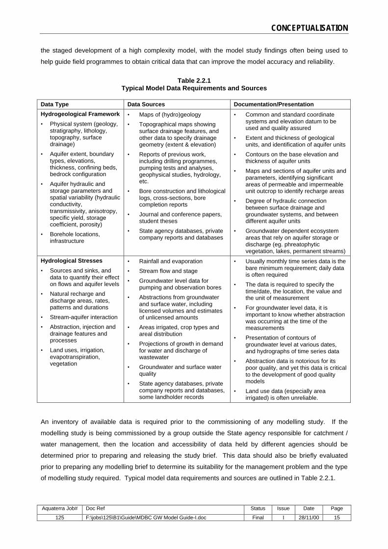
CONCEPTUALISATION



the staged development of a high complexity model, with the model study findings often being used to

help guide field programmes to obtain critical data that can improve the model accuracy and reliability.

Table 2.2.1 Typical Model Data Requirements and Sources

Data Type Data Sources Documentation/Presentation

Hydrogeological Framework

• Physical system (geology, stratigraphy, lithology, topography, surface drainage)

• Aquifer extent, boundary types, elevations, thickness, confining beds, bedrock configuration

• Aquifer hydraulic and storage parameters and spatial variability (hydraulic conductivity, transmissivity, anisotropy, specific yield, storage coefficient, porosity)

• Borehole locations, infrastructure

• Maps of (hydro)geology

• Topographical maps showing surface drainage features, and other data to specify drainage geometry (extent & elevation)

• Reports of previous work, including drilling programmes, pumping tests and analyses, geophysical studies, hydrology, etc.

• Bore construction and lithological logs, cross-sections, bore completion reports

• Journal and conference papers, student theses

• State agency databases, private company reports and databases

• Common and standard coordinate systems and elevation datum to be used and quality assured

• Extent and thickness of geological units, and identification of aquifer units

• Contours on the base elevation and thickness of aquifer units

• Maps and sections of aquifer units and parameters, identifying significant areas of permeable and impermeable unit outcrop to identify recharge areas

• Degree of hydraulic connection between surface drainage and groundwater systems, and between different aquifer units

• Groundwater dependent ecosystem areas that rely on aquifer storage or discharge (eg. phreatophytic vegetation, lakes, permanent streams)

Hydrological Stresses

• Sources and sinks, and data to quantify their effect on flows and aquifer levels

• Natural recharge and discharge areas, rates, patterns and durations

• Stream-aquifer interaction

• Abstraction, injection and drainage features and processes

• Land uses, irrigation, evapotranspiration, vegetation

• Rainfall and evaporation

• Stream flow and stage

• Groundwater level data for pumping and observation bores

• Abstractions from groundwater and surface water, including licensed volumes and estimates of unlicensed amounts

• Areas irrigated, crop types and areal distribution

• Projections of growth in demand for water and discharge of wastewater

• Groundwater and surface water quality

• State agency databases, private company reports and databases, some landholder records

• Usually monthly time series data is the bare minimum requirement; daily data is often required

• The data is required to specify the time/date, the location, the value and the unit of measurement

• For groundwater level data, it is important to know whether abstraction was occurring at the time of the measurements

• Presentation of contours of groundwater level at various dates, and hydrographs of time series data

• Abstraction data is notorious for its poor quality, and yet this data is critical to the development of good quality models

• Land use data (especially area irrigated) is often unreliable.

An inventory of available data is required prior to the commissioning of any modelling study. If the

modelling study is being commissioned by a group outside the State agency responsible for catchment /

water management, then the location and accessibility of data held by different agencies should be

determined prior to preparing and releasing the study brief. This data should also be briefly evaluated

prior to preparing any modelling brief to determine its suitability for the management problem and the type

of modelling study required. Typical model data requirements and sources are outlined in Table 2.2.1.

CONCEPTUALISATION



This data review may redefine the study objectives or initiate data collection networks that are tailored and

specific to the management issue and the required modelling study.

The selected modelling approach should be consistent with the available data sets and the current

conceptual model of the groundwater system. The model should also be flexible enough to be expanded

or refined into a more complex model if more data becomes available and the model is to be used for long

term management of the catchment or aquifer system.

Following the initial hydrogeological interpretation, a computer model may be developed by inputting data

to groundwater modelling software, which is essentially a complex, three-dimensional, interactive

database, with time variability. The project team (project manager, modeller, end-user, community) needs

to assess whether the available data sources are sufficient to achieve the desired study objective and/or

model complexity. If the assessment conclusion is that there is insufficient data or understanding, then

the choices are to:

• Acquire additional data to support the study objective/complexity

• Reduce the model complexity or commit to staged model development from low complexity to the

desired level

• Conclude that a modelling study is not warranted for the time being.

The process of collating data into a form for input to a model usually identifies data gaps, which can be

used to guide monitoring efforts, or to modify the modelling objectives to establish achievable outcomes

for the available level of data and understanding. The associated data analysis often provides an

improved understanding of the groundwater flow system, and is often overlooked and under-resourced in

the rush to develop a model.

G2.2 Recommended guidelines for data collation and initial hydrogeological interpretation:

(a) The available reports on the study area should be collated and listed by the project manager and a

broad description of the essential features of the hydrogeological system outlined in the study

brief. The brief should also identify and list data sources, types and quality, and known issues that

may affect the selection of an appropriate model complexity and the setting of calibration accuracy

targets.

(b) The modelling study should be initiated with a literature review and data analysis in order to

develop an understanding of the important aspects of the physical system, data reliability, and of

the hydrological processes that control or impact the groundwater flow system. The data analysis

should identify data gaps that may affect the model development, and recommend field

programmes necessary for additional data acquisition. The initial literature review and data

analysis step needs to be adequately resourced for the purposes of the modelling study.

(c) The available data to be used in model input or in calibration assessment should be collated into a

database (spreadsheet format as a minimum).

CONCEPTUALISATION



2.3 CONSISTENT DATA UNITS

To be able to be used in a modelling study, all data must be specified in consistent space and time units

(metres and days are accepted standard modelling practice), and to a consistent horizontal and vertical

datum. In addition, it is necessary for aquifer head measurements to be reduced to a common datum

density (eg. fresh water), and to a standard temperature of 25°C (if temperature differences are

significant), so that resulting heads can be contoured meaningfully. The need for consistent units and

datum usually means that surveying of bores and other features is required before data compilation can

be completed.

The applicable elevation datum is almost invariably Australian Height Datum (AHD), which is the standard

datum for published mapping. Mean sea level is represented by 0mAHD (approximately). Any modelling

study, but especially one involving a site close to the coast, however, needs to confirm that the elevation

datum for all data is tied to consistent datum (preferably AHD). This is particularly important for tide data,

which usually forms a boundary condition for coastal models, and can involve more than one chart datum.

Chart datum is rarely tied to AHD, unless a specific survey is completed, and surveys of infrastructure

(bores, roads, wastewater plants, etc.) in coastal areas are often tied to chart datum rather than AHD.

The applicable national spatial datum for maps issued prior to 1996 is Australian Geodetic Datum (AGD).

This datum is currently in the process of being changed to Geocentric Datum of Australia (GDA). GDA

has its origin at the centre of the earth, and is more suited to satellite based navigation systems such as

the Global Positioning System (GPS). The change is planned to be completed by 2000, and generally

results in a change to coordinates of about 200 metres in a north-easterly direction. More information on

GDA is available from www.anzlic.org.au/icsm/gda or www.auslig.gov.au/ausgda/gdastrat.htm.

The old AGD was designed to specifically fit the Australian region, and was measured in Australian Map

Grid (AMG) coordinates for specified zones of six degrees width, with a false origin derived from the

equator and the central meridian through the zone. When model boundaries straddle two zones,

problems occur in matching AMG coordinates at the boundary of the zones.

The move to GDA will not resolve these problems. It is recommended that modellers use a conical equal

area projection (such as Alber’s Projection used in the Great Artesian Basin model), or use a temporary

extrapolation of AMG or GDA coordinates from the major zone to the minor zone. The latter can be

achieved by converting an AMG or GDA coordinate for the minor zone to latitude and longitude, then

converting from latitude and longitude to the AMG or GDA coordinate for the major zone.

Systematic collection of groundwater data or transfer between agencies and individuals is facilitated by

the Australian National Groundwater Data Transfer Standard, introduced in 1999 by the National

Groundwater Committee. The standard can be accessed at www.brs.gov.au/land&water/groundwater/.

CONCEPTUALISATION



G2.3 Recommended guidelines for consistent data units:

(a) Spatial coordinate and elevation data must be specified to a consistent standard datum.

(b) Head measurements should be reduced to a common density (freshwater is suggested) and

common temperature (25°C is suggested) datum.

(c) Data with a length component should be specified in units of metres.

(d) Data with a volume component should be specified in units of cubic metres.

(e) Data with a time component should be specified in units of days.

(f) Database compilations must explicitly state the units of the data.

2.4 DEVELOP CONCEPTUAL MODEL

Development of a valid conceptual model is the most important step in a computer modelling study.

A conceptual model is a simplified representation of the essential features of the physical hydrogeological

system, and its hydrological behaviour, to an adequate degree of detail. The conceptual model is usually

presented graphically as a cross-section or block diagram (eg. Figures 2.4.1 and 2.4.2), with supporting

documentation outlining in descriptive and quantitative terms the essential system features (Table 2.4.1).

It forms the foundation upon which the interactive, site-specific model is built, and is itself based on an

initial literature review, data collation and hydrogeological interpretation (refer Section 2.2).

While the conceptual model is an idealised summary of the current understanding of catchment

conditions, and the key aspects of how the flow system works, it is subject to some simplifying

assumptions. The assumptions are required partly because a complete reconstruction of the field system

is not feasible, and partly because there is rarely sufficient data to completely describe the system in

comprehensive detail. However, the conceptual model should be developed using the principle of

simplicity (or parsimony), such that the model is as simple as possible, while retaining sufficient complexity

to adequately represent the physical elements of the system, and to reproduce system behaviour.

The principle of simplicity/parsimony is also known as Ockham’s Razor - “Entia non sunt multiplicanda

sine necessitate”. This may be translated literally as “The number of entities should not be increased

without good reason”, or loosely as “It is vain to do with more what can be done with fewer” (Constable et

al., 1987). This principle dates from the early 14th Century, and is fundamental to many aspects of life.

In developing an adequate (parsimonious) conceptual model, however, sufficient degrees of freedom must

be incorporated to the model features to allow simulation of a broad range of responses. It must be

possible for the model to predict system responses ranging from desired to undesired outcomes. In other

words, the model must not be configured or constrained such that it artificially produces a restricted range

of prediction outcomes.

CONCEPTUALISATION



Figure 2.4.1 - Typical cross-section type conceptual model

CONCEPTUALISATION



Irrigation areaor wetland/GDE

Layer 1(Superficial deposits)

Layer 2(Sandstone)

Layer 3(Basement)

River

WaterTable

Abstractions

Fault

RainfallRecharge

GroundwaterInflow

GroundwaterOutflow

Evapotranspiration

River inflow

RiverOutflow

Figure 2.4.2 Typical block diagram type conceptual model

Each of the conceptual model features needs to be described to a level of detail commensurate with the

ability of the data to represent the system, and with our ability to understand the system (given the current

data). Our understanding of the system improves as more data are gathered and analysed, and with

assessment of how the system responds to stresses induced by climatic, hydrologic and human-induced

changes. The conceptual model will evolve with new data, and the first conceptual model developed will

not be the last (Spitz and Moreno, 1996), with improvements achieved by augmenting the data base.

Table 2.4.1

Conceptual Model Features

Feature Description Comment

Boundaries Location and type of boundaries for the area to be modelled

Boundary types include specified flow, specified head, and head-dependent flow, as described in Section 2.6.

Geological framework

Geological units, and corresponding hydrostratigraphic units and model layers, and associated aquifer parameters (refer Table 2.2.1). Bedrock configuration and aquifer or aquitard characteristics.

Hydrostratigraphic units comprise geological units with similar aquifer properties. Several geological formations may be combined into one hydrostratigraphic unit (or model layer), or a geological formation may be subdivided into aquifer and confining units (or several layers).

Hydrological framework and stresses

Recharge and discharge processes and dominant aquifer flow mechanisms (Table 2.2.1)

Definition of aquifer media type (porous medium, fractured rock, etc.), and surface-groundwater interaction processes.

Human-induced factors

Anthropogenic influences on the system (Table 2.2.1).

Pumping, irrigation, drainage, weirs, floodways, land clearing, aquifer storage and recovery, waste discharge, mining, etc.

CONCEPTUALISATION



When post-audits are undertaken some years after modelling studies are completed, one of the key

causes of inaccurate predictions has been found to be that the conceptual model is invalid or incomplete

(Anderson and Woessner, 1992) [the other key element is inaccuracies in the assumed future stresses

(pumping rates, rainfall recharge, etc.), and this aspect of uncertainty is dealt with in more detail in Section

5.4]. If a conceptual model inadequately configures certain features (ie. is invalid), or does not incorporate

important features due to lack of data or understanding (ie. is incomplete), then the model application will

not make accurate predictions. Such failures, however unavoidable at the time or understandable in

hindsight, are generally not due to numerical or theoretical deficiencies in the model itself, provided the

model selection (Section 2.5) is valid for the particular problem. Such failures are usually attributable to

errors in the conceptual model, or the assumed stresses, which highlights the importance of these aspects

of modelling.

Often, models are developed in “crisis” mode to answer pressing questions so that management decisions

can be made (Anderson and Woessner, 1992). This particularly applies to low and medium complexity

models, often where the data available may be quite limited, and such an approach may be appropriate

for those studies. However, high complexity models should be developed in “management” mode,

allowing successive improvements to be made to the model, based on augmenting the data base. With

refinements to the conceptual model and improved calibration to a wider range of hydrological conditions

over an extended simulation timeframe, the accuracy and reliability of model predictions will improve.

The definition of a water budget and associated boundary conditions for the model domain are integral

components of the conceptual model. The water budget is a description of the inflows and outflows

across the model domain boundaries, along with any internal consumptive uses, in descriptive and

quantitative terms where possible. The model domain covers the entire area of interest, including areas of

potential future impact, although its size should be minimised to reduce computational effort. Model

boundaries are the interface between the model calculation domain and the surrounding environment

(Spitz and Moreno, 1996), and occur notably on the edges of the domain. Other (“internal”) boundary

conditions reflect influences from other environmental factors (such as rivers, wells, etc.) that are manifest

inside the domain. The external boundaries of the model domain should take advantage of natural or

physical groundwater boundaries (eg. aquifer extents, coastlines, rivers, lakes).

A conceptual model needs to be developed and documented in the Model Study Plan (refer Section 2.6),

and then subject to review by the client, appropriate government agency representatives and the study

reviewer (refer Section 7). The review may result in the need to revise or refine the conceptual model

prior to the initiation of the model construction and calibration tasks. Graphics and descriptive text should

be used to present the conceptual model, so that all parties have the opportunity to assess whether it is

considered valid and complete for the purposes of the study.

CONCEPTUALISATION



G2.4 Recommended guidelines for conceptual model development:

(a) A conceptual model must be developed, presented and reviewed prior to undertaking model

construction, calibration and prediction. Assumptions must be documented.

(b) The conceptual model should be based on an initial literature review, data collation and

hydrogeological interpretation (refer Section 2.2). It should be developed by making use of the

principle of simplicity/parsimony to ensure the model is not too complex for the purposes of the

study.

(c) The conceptual model should present in descriptive and quantitative terms the essential system

features outlined in Table 2.4.1 (geological framework and boundaries), and the hydrological

behaviour (natural and human-induced stresses), including a preliminary water balance.

(d) The conceptual model must have sufficient degrees of freedom to allow a broad range of

prediction responses spanning the criteria of acceptable or unacceptable impacts.

(e) The conceptual model features must be described to an adequate level of detail commensurate

with the ability of the data to represent the system, and with the collective ability to understand the

system, given the current data and likely future data acquisition.

(f) The conceptual model should be documented in a Model Study Plan (Section 2.6), using graphical

representations and descriptive text, and should be subject to review by the client and appropriate

government agency representatives, before initiating model construction and calibration.

(g) The conceptual model should be reviewed and revised as the database is augmented.

2.5 SELECT MODELLING CODE

The modelling code is the computer programme that contains algorithms to numerically solve the

mathematical model. Most modelling codes in common use today also have a graphical user interface

(see later) for the pre- and post-processing of modelling data.

The mathematical model is the basic hydraulic equation that governs the flow of groundwater in the

saturated zone. It is a partial differential equation in time and three-dimensional space. The conceptual

model and the hydrogeological framework data together help to define the boundary conditions for the

solution of the mathematical model. The hydrogeological stresses complete the boundary condition

definition, and provide the temporal and spatial data for the solution of the hydraulic equation.

A modelling code can be thought of as a very complex, three-dimensional, interactive database, with time

variability, because it incorporates the following:

• the means to input data to describe the model domain and hydrologic stresses in space and time

• the numerical algorithms to solve the mathematical model (hydraulic equation of groundwater flow)

• the means to output the results of the simulation.

CONCEPTUALISATION



Most mathematical models use analytical (simple) or numerical (complex) means to solve the governing

differential equations. There are other methods, such as the boundary integral method (a combination of

analytical and numerical methods), and the analytical element method (an elaborate semi-analytical

method), but they are not in common use in Australia.

Analytical models are equations representing exact solutions to the hydraulic equation for one- or two-

dimensional flow problems under broad simplifying assumptions, usually including aquifer homogeneity.

They can be solved by hand, or by simple computer programs (eg. WinFlow, TwoDan), but do not allow

for spatial variability and often do not allow for temporal variability. They are useful to provide rough

approximations for many applications with little effort, as they usually do not involve calibration (site-

specific monitoring data is often not available for these simple problems). This approach can suit most

simple, low-complexity modelling studies. There is no systematic approach for simplifying a given

groundwater problem and for selecting the appropriate analytical solution. In fact, it depends entirely on

the capability of the model user to visualise the problem and to apply professional judgement to select a

valid analytical approach.

In numerical models, the continuous differential terms in the governing equations are replaced by finite

quantities. The computational power of the computer is used to solve the resulting algebraic equations by

matrix arithmetic. In this way, problems with complex geometry, dynamic response effects and spatial and

temporal variability may be solved accurately. This approach must be used in cases where the essential

aquifer features form a complex system, and where surface-groundwater interaction is an important

component. To facilitate the data input, flow simulation and results output, most computer modelling

codes in common use provide a graphical user interface (GUI), based on the Microsoft Windows system.

Examples of commonly used numerical codes and graphical user interfaces are outlined in Appendix D.

These codes are in common use (but are not the only ones used) for groundwater flow modelling, but they

are not necessarily superior or inferior to other codes not shown in the tables in Appendix D.

The selection of an appropriate modelling code and GUI for a particular study is a matter of ensuring that

the code has the capability to adequately represent the essential features and flow processes of the

groundwater system being studied. It is also important to ensure that the selected code has been verified

and benchmarked against standard test problems, to confirm that the code accurately solves the

equations that comprise the mathematical model. Most of the commercially available codes (including

those in Appendix D) have been verified, but it is still worthwhile for the modeller to run test problems to

confirm that the modelling software installation on their PC can reproduce the test problem simulation

results accurately. Other factors (Table 2.5.1) should be considered when selecting an appropriate

modelling code, and documented by the modeller in the Modelling Study Plan (next Section).

Public domain modelling codes are often preferred to proprietary codes. Public domain codes are defined

here as commercially available and widely distributed, relatively inexpensive, and generally accepted

models with features that can be and have been used to simulate a wide range of hydrogeological

conditions. Public domain codes (eg. including many listed in Appendix D) have received extensive peer

review, and case histories documenting their general applicability, as well as their limitations, have been

CONCEPTUALISATION



published in the scientific literature. Many were originally developed (and are continually being refined) by

US government agencies (eg. US Geological Survey, EPA and Dept of Defense), with substantial

assistance from specialist consultants. Proprietary codes are those developed in-house by certain

companies, and while they may share many attributes with public domain codes, the source code

programme is not available, the purchase price is usually much more expensive, and the peer review is

often limited.

Issues to be considered when considering public domain versus proprietary models include:

• if the project is funded by government agencies, and is regarded as public information, all aspects may

need to be available for public review;

• proprietary codes may need to be purchased for future use on a specific study, adding to the overall

costs of a project, whereas public domain codes are usually already available in most organisations

• for future simulation work the client may be required to engage the consultant who owns the proprietary

code, and may not be able to request competitive bids;

• if a proprietary code is purchased, the client will probably need to recruit staff and/or commit resources

for training in the specifics of the programme.

It is generally accepted that Modflow, originally developed by the US Geological Survey (McDonald and

Harbaugh, 1996), is the industry-leading public domain numerical flow model, although it is not necessarily

suitable for every modelling study. There are a number of graphical user interfaces for Modflow, for which

brief summaries are provided in Appendix D, along with a table of the minimum aquifer parameter data

requirements for this model. There are also several text books that detail modelling methodologies with

Modflow (notably Anderson and Woessner, 1992), and there are regular conferences held in the USA on

Modflow projects.

The main reasons that Modflow enjoys a good reputation are that the code has been verified against a

range of analytical solutions, it has been used to successfully simulate a wide range of hydrogeological

systems across the world, the source code is in the public domain and there are several relatively cheap

GUIs available (some good GUIs are available for free – eg. Processing Modflow for Windows PMWin4

can be downloaded from www.uovs.ac.za/igs/index.htm).

Another great strength is that the Modflow code was developed with a modular structure (eg. modules for

certain hydrological processes may be turned on or off), and new modules for flow processes or improved

numerical methods are being continually produced and integrated seamlessly. Modflow is known to have

the best range of stream-aquifer interaction modules. For these and other reasons, organisations such as

the UK Environment Agency have adopted Modflow as the preferred modelling package for their regional

models.

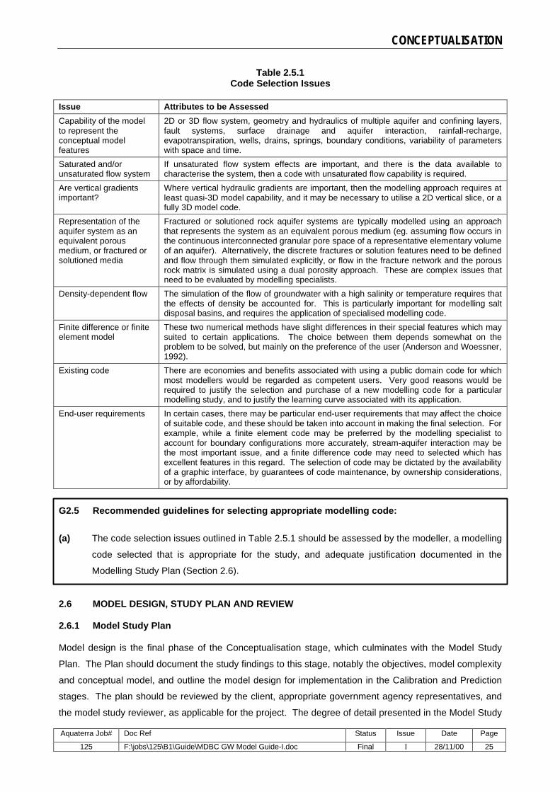
CONCEPTUALISATION



Table 2.5.1 Code Selection Issues

Issue Attributes to be Assessed

Capability of the model to represent the conceptual model features

2D or 3D flow system, geometry and hydraulics of multiple aquifer and confining layers, fault systems, surface drainage and aquifer interaction, rainfall-recharge, evapotranspiration, wells, drains, springs, boundary conditions, variability of parameters with space and time.

Saturated and/or unsaturated flow system

If unsaturated flow system effects are important, and there is the data available to characterise the system, then a code with unsaturated flow capability is required.

Are vertical gradients important?

Where vertical hydraulic gradients are important, then the modelling approach requires at least quasi-3D model capability, and it may be necessary to utilise a 2D vertical slice, or a fully 3D model code.

Representation of the aquifer system as an equivalent porous medium, or fractured or solutioned media

Fractured or solutioned rock aquifer systems are typically modelled using an approach that represents the system as an equivalent porous medium (eg. assuming flow occurs in the continuous interconnected granular pore space of a representative elementary volume of an aquifer). Alternatively, the discrete fractures or solution features need to be defined and flow through them simulated explicitly, or flow in the fracture network and the porous rock matrix is simulated using a dual porosity approach. These are complex issues that need to be evaluated by modelling specialists.

Density-dependent flow The simulation of the flow of groundwater with a high salinity or temperature requires that the effects of density be accounted for. This is particularly important for modelling salt disposal basins, and requires the application of specialised modelling code.

Finite difference or finite element model

These two numerical methods have slight differences in their special features which may suited to certain applications. The choice between them depends somewhat on the problem to be solved, but mainly on the preference of the user (Anderson and Woessner, 1992).

Existing code There are economies and benefits associated with using a public domain code for which most modellers would be regarded as competent users. Very good reasons would be required to justify the selection and purchase of a new modelling code for a particular modelling study, and to justify the learning curve associated with its application.

End-user requirements In certain cases, there may be particular end-user requirements that may affect the choice of suitable code, and these should be taken into account in making the final selection. For example, while a finite element code may be preferred by the modelling specialist to account for boundary configurations more accurately, stream-aquifer interaction may be the most important issue, and a finite difference code may need to selected which has excellent features in this regard. The selection of code may be dictated by the availability of a graphic interface, by guarantees of code maintenance, by ownership considerations, or by affordability.

G2.5 Recommended guidelines for selecting appropriate modelling code:

(a) The code selection issues outlined in Table 2.5.1 should be assessed by the modeller, a modelling

code selected that is appropriate for the study, and adequate justification documented in the

Modelling Study Plan (Section 2.6).

2.6 MODEL DESIGN, STUDY PLAN AND REVIEW

2.6.1 Model Study Plan

Model design is the final phase of the Conceptualisation stage, which culminates with the Model Study

Plan. The Plan should document the study findings to this stage, notably the objectives, model complexity

and conceptual model, and outline the model design for implementation in the Calibration and Prediction

stages. The plan should be reviewed by the client, appropriate government agency representatives, and

the model study reviewer, as applicable for the project. The degree of detail presented in the Model Study

CONCEPTUALISATION



Plan should be appropriate for the specified model complexity, and it should be sufficiently detailed that

another modeller could undertake future stages of the model development.

Discussion of issues relating to the first three points in the guideline below have been presented in

previous sections. The model configuration specifics are discussed below.

G2.6 Recommended guidelines for Model Study Plan:

A Model Study Plan should be completed and reviewed at the end of the Conceptualisation stage

with a report that includes details of the:

1. study purpose, objectives, model complexity, and resources required to complete the study

2. initial hydrogeological interpretation and conceptual model, data summary, boundary

conditions and preliminary water budget

3. selected modelling code and limitations/uncertainties in the modelling approach

4. model design and configuration specifics (as outlined in Sections 2.6.2 to 2.6.11), including

details on the boundaries; grid; layers; aquifer units and parameters; recharge, discharge and

water balance; surface-groundwater interaction; calibration and prediction timeframes and

accuracy targets; steady state or transient calibration and/or prediction runs; and data

available and required to complete the study

5. for high complexity models, it may be appropriate to document the data collated by

presenting the database in the Model Study Plan report (eg. in tables or appendices, or

possibly on a CD for archive purposes).

2.6.2 Boundary Conditions

Boundary conditions are constraints imposed on the model grid to represent the interface between the

model calculation domain and the surrounding environment. There are three major types of boundary

conditions (Table 2.6.1), all of which may vary with time. The type of boundary selected should be

consistent with the conceptual model and the water budget, and should be located and oriented consistent

with the physical features it represents. In particular, model domain boundaries should be set far from the

area of interest (eg. a water supply borefield) so that imposed stresses on the grid interior do not reach the

boundaries. Alternatively, the boundary needs to be configured such that the simulated boundary effect is

realistic (eg. using a head-dependent flow boundary at a groundwater divide or a surface-groundwater

interaction feature).

Boundary conditions should be designed to take advantage of physical or hydraulic boundaries. Physical

boundaries usually relate to the physical presence of an impermeable geological formation or a large body

of surface water. An impermeable boundary typically forms the lower and/or lateral boundaries of

modelled systems, and may be justified provided there is at least a two order of magnitude contrast in

hydraulic conductivity between the two units (Anderson and Woessner, 1992). Hydraulic boundaries form

as a result of hydrologic conditions, notably at groundwater divides and streamlines, although these

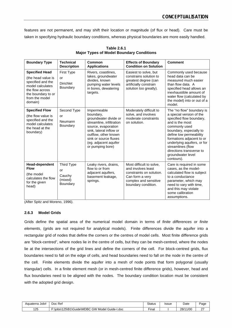
CONCEPTUALISATION



features are not permanent, and may shift their location or magnitude (of flux or head). Care must be

taken in specifying hydraulic boundary conditions, whereas physical boundaries are more easily handled.

Table 2.6.1 Major Types of Model Boundary Conditions

Boundary Type Technical

Description Common Applications

Effects of Boundary Condition on Solution

Comment

Specified Head

(the head value is specified and the model calculates the flow across the boundary to or from the model domain)

First Type

or

Dirichlet Boundary

Rivers, coastlines, lakes, groundwater divides, known pumping water levels in bores, dewatering targets.

Easiest to solve, but constrains solution to greatest degree (can artificially constrain solution too greatly).

Commonly used because head data can be measured much easier than flow data. A specified head allows an inexhaustible amount of water flow (calculated by the model) into or out of a model.

Specified Flow

(the flow value is specified and the model calculates the head at the boundary)

Second Type

or

Neumann Boundary

Impermeable boundary, groundwater divide or streamline, infiltration source, evaporation sink, lateral inflow or outflow, other known sink or source fluxes (eg. adjacent aquifer or pumping bore)

Moderately difficult to solve, and involves moderate constraints on solution.

The “no flow” boundary is a special version of the specified flow boundary, and is the most commonly used boundary, especially to define low permeability formations adjacent to or underlying aquifers, or for streamlines (flow directions transverse to groundwater level contours).

Head-dependent Flow

(the model calculates the flow for the given head)

Third Type

or

Cauchy (mixed) Boundary

Leaky rivers, drains, flow to or from adjacent aquifers, basement leakage, springs.

Most difficult to solve, and involves least constraints on solution. Can form a very complex and sensitive boundary condition.

Care is required in some cases, as the model-calculated flow is subject to a conductance parameter, which may need to vary with time, and this may violate some calibration assumptions.

(After Spitz and Moreno, 1996).

2.6.3 Model Grids

Grids define the spatial area of the numerical model domain in terms of finite differences or finite

elements, (grids are not required for analytical models). Finite differences divide the aquifer into a

rectangular grid of nodes that define the corners or the centres of model cells. Most finite difference grids

are “block-centred”, where nodes lie in the centre of cells, but they can be mesh-centred, where the nodes

lie at the intersections of the grid lines and define the corners of the cell. For block-centred grids, flux

boundaries need to fall on the edge of cells, and head boundaries need to fall on the node in the centre of

the cell. Finite elements divide the aquifer into a mesh of node points that form polygonal (usually

triangular) cells. In a finite element mesh (or in mesh-centred finite difference grids), however, head and

flux boundaries need to be aligned with the nodes. The boundary condition location must be consistent

with the adopted grid design.

CONCEPTUALISATION



The spatial discretisation of the grid should be fine in areas of interest or areas of stress, but may be

coarse away from these areas, or where data are sparse. The size of the nodal spacing is dependent on

the expected curvature of the water table or potentiometric surface, with fine spacing required to

accurately define highly curved surfaces (eg. around pumping wells or near rivers, etc.) or steep hydraulic

gradients in the horizontal or vertical directions. Nodes may be regularly spaced, or the spacing may be

increased as the grid is expanded towards regional boundaries. For finite difference grids, the grid

expansion factor (ratio of larger to smaller adjacent nodal spacings) should not exceed 1.5. The aspect

ratio (ratio of maximum to minimum cell dimensions) should ideally be close to unity, and should not

exceed 10 for finite difference grids, or a value of 5.0 for finite element meshes (Anderson and Woessner,

1992).

The external boundaries of the model domain should be oriented parallel to the primary groundwater flow

direction if possible. Often, particularly for regional models with variable flow direction, it is more

convenient to align a model grid with cardinal directions.

2.6.4 Layers

Layers are used in models to represent hydrostratigraphic units, which comprise geological units with

similar aquifer properties. Several geological formations may be combined into one hydrostratigraphic unit

(or model layer), or a geological formation may be subdivided into aquifer and confining units (or several

layers). Quasi-3D (multi-layer) models usually simulate horizontal flow in each of the stacked aquifer

layers, and vertical leakage through confining units between layers. Aquifer head and storage is often not

simulated in the confining unit. This is considered an acceptable approximation when there is more than

two orders of magnitude contrast in hydraulic conductivity between the aquifer and confining units

(Anderson and Woessner, 1992). Otherwise, a profile model (see below) or a fully-3D model may be

preferred. However, fully-3D models have more onerous data requirements, and expert advice is required.

The number of layers in a model will depend on the conceptualisation of the aquifer system and on all of

the factors which define a model’s complexity (Section 2.1). More layers are needed when vertical head

gradients are significant, as the head in each model layer is effectively averaged over the thickness of that

layer. Figures 2.4.1 and 2.4.2 provide examples of model layer configurations.

Layer elevation data (top and bottom surfaces or layer thickness) are a key data requirement for models,

to define aquifer thickness, and therefore help define aquifer transmissivity (product of hydraulic

conductivity and thickness) and storage volumes. Geometry is also used when the top elevation of a layer

is compared in the mathematical model to the simulated water level to decide whether the aquifer at that

point is confined or unconfined, while the bottom elevation is used to identify when a cell is drained (“goes

dry”), or should be “re-wet”. If it is known beforehand that the aquifer is confined, and the saturated

thickness will not vary significantly through simulations, then substantial data processing savings can be

made by not specifying layer elevations, and modelling the confined aquifer using the transmissivity

parameter. For unconfined aquifers, however, and any dewatering-type simulations, or where the

saturated thickness varies significantly, it is critical to define the layer geometry as accurately as possible.

CONCEPTUALISATION



2.6.5 Profile Models

Profile or slice models consist of two-dimensional models oriented vertically, and are used when vertical

flows or vertical hydraulic gradients are important, but a fully-3D model may not be warranted. A profile

model is usually a vertical slice of unit width of aquifer, which must be oriented along a flow-line to remain

consistent with the assumption of conservation of mass. As more layers can be accommodated in a

profile model (than an areal model) for the same level of computational demand, profile models are

suitable for situations in which detailed simulation of vertical flow components is essential. Point sinks and

sources (eg. wells) cannot be accurately simulated in a profile model, as they represent radial flow

features, and a profile model cannot account for components of flow outside the cross-section. Line sinks

or sources (ie. a long linear feature such as a river or drain aligned transverse to the profile) can be

simulated in a standard profile model. An axi-symmetric profile model (in simple terms, a wedge-shaped

slice of aquifer) can be used to simulate point sinks or sources, although this requires special computer

codes and techniques.

Layers may correspond with undulating geological units, or they may be horizontal slices in which the

lithological variation is handled by variable aquifer properties along the layer.

2.6.6 Aquifer Units and Parameters

Parameter values need to be assigned to the appropriate models cells, based on the extent of the

corresponding hydrostratigraphic units, and the associated field measurements or literature estimates for

the aquifer parameters. This is where Graphical User Interface (GUI) software packages (Appendix D)

have improved modelling productivity by making data processing more manageable. Typically, parameter

data are sparse, and some form of interpolation is required to represent the overall spatial variability of

aquifer parameters over the model domain based on a few point measurements. Geostatistical methods

are sometimes used, and automated calibration techniques (notably using PEST software (Doherty,

1994), and http://www.ozemail.com.au/%7Ewnc/) are becoming much more popular methods for

accounting for spatial parameter variability, while reducing the model calibration effort. This is discussed

further in Chapter 3.

2.6.7 Water Budget

The preliminary water budget should be outlined in terms of the major components of natural recharge

and discharge, and human-induced stresses (abstraction and seepage). The locations where these inputs

and outputs are manifest must be detailed, along with known or expected changes with time (due to

climatic variations, pumping, seepage and surface-groundwater interaction).. The water budget needs to

be viewed in conjunction with the conceptual model to estimate the overall throughputs of water through

the groundwater system. The initial estimates should be cross-checked with subsequent modelling

estimates of long term and short term water budget components.

CONCEPTUALISATION



2.6.8 Surface-Groundwater Interaction

Surface-groundwater interaction can form a critical component of the water budget, as well as an essential

feature of the conceptual model, and often forms the most complex, sensitive and uncertain parts of a

model. This is particularly so because the relevant flow processes commonly involve consideration of

unsaturated flow, recharge and evapotranspiration processes. Detailed consideration of these issues is

outside the scope of this work, but some discussion on more general aspects is given below.

There are analytical solutions covering a range of surface-groundwater interaction conditions, although

rigid boundary conditions and simplifying assumptions mean that these analytical models can usually only

be applied to simple one-dimensional problems. A full discussion of analytical techniques is not within the

scope of this guideline, although a good summary is provided in the US Army manual (USACE, 1999),

which is available on-line (refer Appendix A for details).

Dynamic simulation of surface-groundwater interaction requires mathematical description of transient

effects within complex surface and groundwater flow systems, such as:

• rainfall-runoff processes, surface water flow routing, and evapotranspiration

• fluctuations in the stage (elevation) and volume of a surface water body, and leakage to groundwater

• infiltration through the ground surface and flow in the unsaturated (vadose) zone

• flow in the saturated (aquifer zone) and discharge to the ground surface.

From a groundwater perspective, it is commonly assumed that direct simulation of the unsaturated flow

system is not critical, and that leakage from surface water to groundwater occurs instantaneously. As

most groundwater models utilise a one month stress period, this approximation is usually valid. In some

cases, however, these assumptions will not be valid, and specialised treatment of surface-groundwater

interaction process will be required, using specialised computer code, and modelling expertise. For most

groundwater modelling projects, however, the treatment of surface-groundwater interaction is effected by

utilising the major boundary conditions types (Table 2.4.1), based on appropriate simplifying assumptions,

which will vary for the site-specific conditions involved. The method adopted for any particular case

should be as simple as possible or as complex as necessary, appropriate for the study purpose,

complexity and data available.

The simplest approaches involve the use of specified head and specified flow boundaries, while more

complex approaches involve head-dependent flow boundaries, which also sometimes account for surface

flow volumes. With specified head boundaries, the aquifer head at the surface water location is commonly

specified as the elevation of the water surface, and the model computes the flow across the boundary,

dependent on the gradient to or from the adjacent model cells. With specified flow boundaries, the flow

rate across the boundary is specified as a “known” value, and the model computes the corresponding

head value at the boundary. Both of these approaches can be used to simulate a range of surface-

groundwater interaction processes, including rivers, drains, springs, lakes, coastlines, evapotranspiration,

etc. Both of these approaches, however, suffer from the limitations that the hydraulic conductivity across

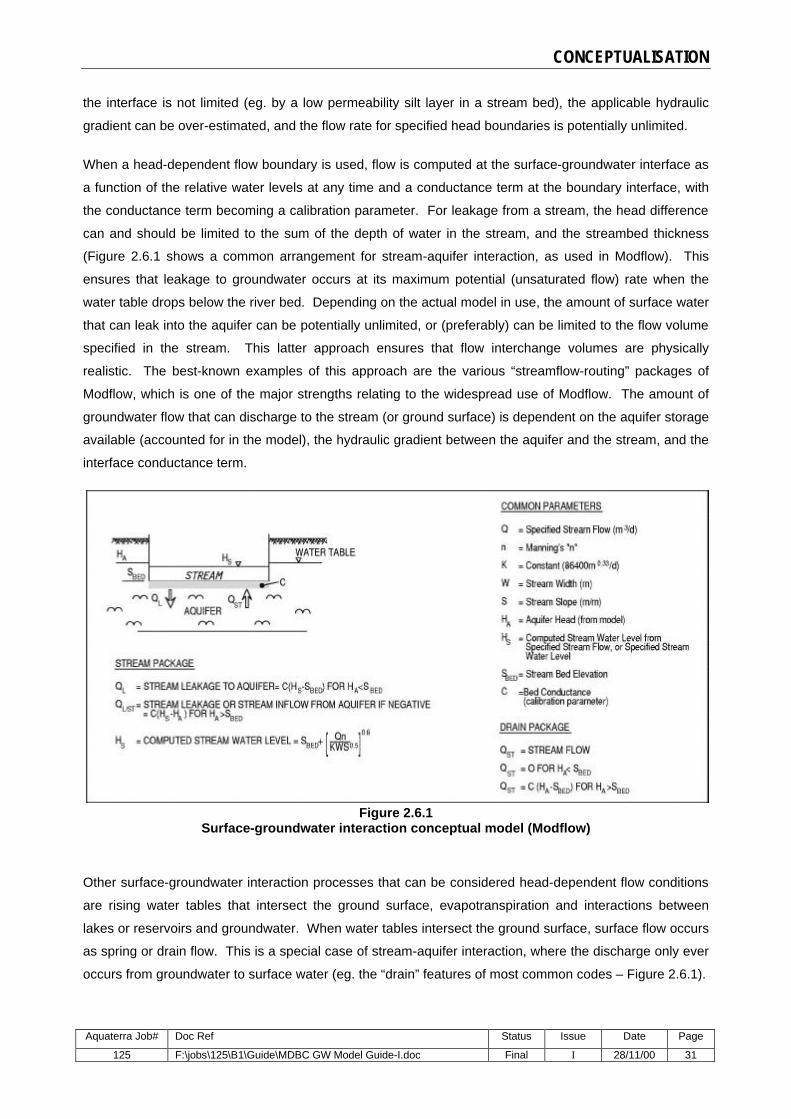
CONCEPTUALISATION



the interface is not limited (eg. by a low permeability silt layer in a stream bed), the applicable hydraulic

gradient can be over-estimated, and the flow rate for specified head boundaries is potentially unlimited.

When a head-dependent flow boundary is used, flow is computed at the surface-groundwater interface as

a function of the relative water levels at any time and a conductance term at the boundary interface, with

the conductance term becoming a calibration parameter. For leakage from a stream, the head difference

can and should be limited to the sum of the depth of water in the stream, and the streambed thickness

(Figure 2.6.1 shows a common arrangement for stream-aquifer interaction, as used in Modflow). This

ensures that leakage to groundwater occurs at its maximum potential (unsaturated flow) rate when the

water table drops below the river bed. Depending on the actual model in use, the amount of surface water

that can leak into the aquifer can be potentially unlimited, or (preferably) can be limited to the flow volume

specified in the stream. This latter approach ensures that flow interchange volumes are physically

realistic. The best-known examples of this approach are the various “streamflow-routing” packages of

Modflow, which is one of the major strengths relating to the widespread use of Modflow. The amount of

groundwater flow that can discharge to the stream (or ground surface) is dependent on the aquifer storage

available (accounted for in the model), the hydraulic gradient between the aquifer and the stream, and the

interface conductance term.

Figure 2.6.1 Surface-groundwater interaction conceptual model (Modflow)

Other surface-groundwater interaction processes that can be considered head-dependent flow conditions

are rising water tables that intersect the ground surface, evapotranspiration and interactions between

lakes or reservoirs and groundwater. When water tables intersect the ground surface, surface flow occurs

as spring or drain flow. This is a special case of stream-aquifer interaction, where the discharge only ever

occurs from groundwater to surface water (eg. the “drain” features of most common codes – Figure 2.6.1).

CONCEPTUALISATION



Special evapotranspiration features are available in some codes that simulate the discharge of

groundwater at a rate that increases with increasing water table level, up to a maximum limit (usually free

water evaporation that applies at the ground surface), as indicated in Figure 2.6.2. This approach can be

used to simulate evapotranspiration from vegetation, as well as from lake features. It can also be used to

simulate otherwise very complex surface-groundwater interaction processes, such as “rejected recharge”

and “interflow” surface discharge during the wet season (eg. in the N.T.) from groundwater systems where

the water table is very close to the ground surface. In this case, there is no conductance term to limit the

flow rate, although the evapotranspiration flux is usually limited to some factor of the pan evaporation rate.

Figure 2.6.2 Evapotranspiration conceptual model (Modflow)

A number of lake and reservoir simulation algorithms have recently become available, which take account

of the water balance interactions for these mini-systems (Figure 2.6.3). The ModelCare 1998 conference

included several papers that concluded that the new, complex algorithms for treating lake-type features

gave quite consistent results compared to the more traditional method (eg. Chung and Anderson, 1998).

The traditional method is to specify lake-cells in models with a storage value of 1.0, and a very high

permeability (say, 10,000m/d), and to also allow for other surface-groundwater interaction fluxes (eg.

evapotranspiration and groundwater inflow/outflow).

Figure 2.6.3 Lake Water Balance Components

Groundwater inflow/outflow

Stream outflow

Stream inflow Surface runoff

Rainfall Evaporation

Lake stage

CONCEPTUALISATION



2.6.9 Timeframes

Two types of time interval are used in flow models:

• stress periods during which boundary conditions and stresses (eg. hydrologic conditions and pumping)

are constant, and between which boundary conditions and stresses can vary; and,

• time steps during which model calculations are made to simulate the effect of stresses on the system.

The definition of suitable stress periods is complicated by the fact that individual hydrological conditions

(eg. rainfall, stream flow and pumping regimes) can vary quite independently, and yet stress periods must

be defined when each of the stresses may be considered constant. This can result in a very complex data

processing operation to prepare model input and process model output files, and appropriate study

resources need to be allowed for this purpose. It is common for monthly stress periods (eg. 30.44 days)

to be adopted, with individual stress rates being averaged, although this can cause problems when

checking model calibration against measured data, which reflects the dynamic response of the system to

the actual (potentially short-lived) stress occurring. Some codes allow separate stress periods for different

types of stress.

Ideally, models should use small time steps to obtain accurate iterative solutions, but this can cause

inefficiencies due to long run times. Time steps may be constant or increasing during a stress period.

The model solution is sensitive to rapidly fluctuating water levels caused by introducing or changing

stresses, and a number of small time steps should be used to capture the early response, even if one is

only interested in the solution at later times.

To guide the selection of time steps, Anderson and Woessner (1992) recommend a minimum critical time

step (Tc = Sa2/4T, where representative values are inserted for storage S, transmissivity T and

cell/element size a). This estimate, however, is very conservative as it is pertinent only to explicit solution

methods. In practice, iterative methods of solution can tolerate a much larger minimum time step, in the

order of 100 times the critical value. A further rule of thumb suggests that the solution should proceed

through at least 3 to 5 time steps, with no significant stress or boundary condition changes, before the

solution is considered accurate. In any case, the sensitivity of the solution to time step changes may need

to be evaluated.

The Model Study Plan should outline:

• how the available data record will be split into calibration and verification data sets;

• how the calibration, verification and prediction periods will be split into stress periods, and how time

steps will be designed to ensure accurate solutions;

• what the prediction timeframe will be, and what hydrological data will be utilised in the prediction

simulations (eg. a repeated cycle of the historical data).

CONCEPTUALISATION



2.6.10 Accuracy Targets

Calibration accuracy targets should be proposed in the Model Study Plan (refer Section 3 for calibration

measures) as measures of the acceptance criteria prior to undertaking model construction and calibration.

The setting of these targets may require some discussion between the modeller and client, and could

possibly involve appropriate government agency representatives and the independent model reviewer.

2.6.11 Resources and Data Required

Based on the details of the Model Study Plan, the resources required to successfully complete the

modelling study (ie. meet the stated objectives and model complexity) should be outlined (in terms of data,

time, budget, staff, etc.), and a staged model development plan proposed.

2.6.12 Review

A report on the Model Study Plan should be prepared and submitted to the client and/or the project team

model reviewer for review prior to undertaking any further work on the model. The report should

document all the model design features mentioned in this section, using the guidelines suggested in

Section 6.

SECTION 3 - CALIBRATION



3.1 CONSTRUCT MODEL

Construction of a groundwater flow model is the process of transforming the conceptual model into a

mathematical form that can be used to simulate groundwater heads and flows. The required outcome is

an interactive model with features to represent the hydrogeological framework, hydraulic properties,

hydrological processes and boundary conditions as designed in the Conceptualisation stage (Section 2).

An interactive model can take the form of an analytical model or numerical model (refer Section 2.5).

Analytical models can be solved using a calculator, a spreadsheet, or a special software package (eg.

WinFlow, TwoDan, etc.), with the study usually being completed within a period of hours to days. They

are based on simplifying assumptions, and usually adopt uniform aquifer parameters and hydrologic

conditions for any one simulation, although a range of analyses should be undertaken to test sensitivity to

various conditions and uncertainty in predictions (Section 5.2). The construction of analytical models is a

simple process, but it still needs to be adequately documented and reviewed if the results will be used to

facilitate important decisions. Analytical models are not exempt from calibration, if sufficient data are on

hand. An unsuccessful calibration could indicate that the conceptual model is too simple.

Numerical model construction is a more complicated and time-consuming process, even when using one

of the many graphical user interfaces (GUIs) available commercially (Appendix D). Essentially, it involves

the design of a model grid, time stepping and model features to represent boundary conditions and stress-

inducing processes (refer Section 2.6), and the initial assignment of time-variant data and time-constant

parameters to the model. This is fundamentally a data processing task that can take up to 20% or more of

the modelling effort, depending on the amount of data involved and the complexity of the system.

Numerical model construction requires that each node or element of the grid or mesh is assigned a value

for each hydrogeological framework property and aquifer hydraulic parameter required for that model

(typical data requirements for a Modflow model are presented in Appendix D). The framework and

hydraulic properties are commonly assigned to hydrostratigraphic units in the model on the basis of

geological and aquifer testing/monitoring data, usually in broad zones with the same geological or aquifer

characteristics. In addition, time-varying hydrological data needs to be applied to those model features

representing stresses on the system (eg. pumping wells, rivers, evapotranspiration, etc.), as described in

Section 2.6.9. Viewed from this perspective, a model can be seen to be a complex, three-dimensional,

interactive database, with time variability, and the data processing task should be resourced in a manner

consistent with the model complexity.

The construction of a model can sometimes require refinements to be made to the conceptual model,

especially if our understanding of certain model features or stresses, or the data available to represent

those aspects, has significant limitations (which is often the case). It is not uncommon for new data to

become available during model construction, and this could impact on the underlying conceptual model.

CALIBRATION



G3.1 Recommended guidelines for model construction:

Any assumptions or modifications required to refine the conceptual hydrogeological understanding

during its transformation into a mathematical model should be fully documented.

3.2 MODEL CALIBRATION PROCESS

3.2.1 General

Calibration is the process by which the independent variables (parameters and fluxes) of a model are

adjusted, within realistic limits, to produce the best match between simulated and measured data (usually

from groundwater level monitoring). In other words, calibration methods solve a problem inversely by

adjusting the unknowns (parameters and fluxes) until the solution matches the knowns (heads). This

process involves refining the hydrogeological framework, hydraulic properties, and boundary conditions of

the model to achieve the desired degree of correspondence between the model simulations and

observations of the groundwater flow system. Calibration is a necessary, but not sufficient, condition that

must be obtained to have a degree of confidence in a model’s predictions (ASTM D5981-96), as it shows

that a model simulation can reproduce system behaviour under a certain set of conditions. A calibration

sensitivity analysis should also be undertaken to assess the relative importance of model parameters in

achieving the calibration result (refer Section 5).

The success of model calibration should be evaluated in both quantitative (statistical) and qualitative

(pattern-matching) terms, to evaluate the degree of correspondence between a simulation and site-

specific information. Quantitative measures usually involve mathematical and graphical comparisons

between measured and simulated aquifer heads, and the calculation of statistics regarding residuals (the

difference between measured and simulated aquifer heads). Quantitative measures can also include

comparison of simulated and measured components of the water budget, notably surface water flows,

groundwater abstractions and evapotranspiration estimates. Qualitative assessment of calibration is

commonly undertaken by comparing patterns of groundwater flow (based on contour plans of aquifer

heads), considering the justification for adopting model aquifer properties in relation to measured ranges

of values, and associated non-uniqueness issues. Qualitative assessment is undertaken with due

consideration for the adopted conceptual model, particularly relating to surface-groundwater interaction.

The initial setup of a mathematical model includes assumed distributions of aquifer parameters such as

hydraulic conductivity, storage coefficient and leakage coefficient. The calibration process varies these

parameters in successive model runs, until field data (eg. heads or flows) match model data reasonably

well. Usually the recharge distribution is also unknown, and this must also be adjusted during calibration.

Traditionally, the calibration process involves the trial-and-error variation of parameters and assessment of

results. This is a very subjective process, modulated by the experience and perseverance of the

individual.

It is important for the modeller to maintain a journal of the trial-and-error calibration process to ensure

systematic progress. In the words of Carrera and Neuman (1986): “The method (of trial-and-error) is

CALIBRATION



recognised to be labour intensive (therefore expensive), frustrating (therefore often left incomplete), and

subjective (therefore biased and leading to results the quality of which is difficult to estimate)”. There is

currently a trend away from trial-and-error to automated calibration, made possible by the incorporation of

inverse estimation software (notably PEST) with convenient graphical user interfaces (refer Appendix D).

Automated calibration highlights the essential non-uniqueness of most modelling applications (see Section

3.2.2). Modellers often either ignore or are not aware of the extent of non-uniqueness lurking beneath a

model calibrated by trial-and-error. Extensive guidelines for automated calibration have been developed

by Hill (1998) (see Appendix A).

G3.2 Recommended guideline for model calibration assessment:

(a) Medium to high complexity models should be calibrated to measured data before they are used for

prediction simulations, and the calibration performance should be presented in qualitative and

quantitative terms in comparison to agreed target criteria.

(b) A calibration sensitivity analysis should be undertaken (refer Section 5).

(c) A journal of the calibration process should be kept.

G3.2 Recommended guideline for automated model calibration

(d) Since an objective function is used to compare how the model simulation matches the historical

groundwater system behaviour, the formulation of the objective function is a critical step in

automated model calibration and should be discussed and justified. The objective function should

be sensitive to deviations from calibration targets.

(e) Automated model calibration should be preceded by a manually-instigated calibration effort to

check that the mathematical model is in fact performing correctly in terms of data accuracy and

conceptual functionality.

(f) An inverse model (eg. PEST, UCODE or MODFLOWP) should be run for one iteration initially to

identify the correlated parameters and insensitive parameters. One of the correlated parameters

and the insensitive parameters should be fixed before the automated model calibration is to

proceed.

3.2.2 Non-uniqueness Problem

The non-uniqueness problem arises because many different possible sets of model inputs can produce

nearly identical model outputs. In other words, multiple calibrations of the same system are possible using

different combinations of boundary conditions and aquifer properties, because exact (“unique”) solutions

cannot be computed when many variables are involved in the calibration approach. It can be shown that

any combination of groundwater flow rates and hydraulic conductivities in the model that has the same

ratio as the actual flow rates and hydraulic conductivities in the aquifer will produce nearly identical

CALIBRATION



hydraulic head distributions (Ritchey and Rumbaugh, 1996). This is shown heuristically in Figure 3.2.1,

along with annotations to illustrate techniques (described below) that can be used to reduce the non-

uniqueness problem. The apparent matching of measured aquifer heads at a certain date by a

“calibrated” model does not necessarily mean that the hydraulic properties used in the model are close to

those actually found on site, although obtaining correct predictions does depend strongly upon using the

correct properties.

Figure 3.2.1 Addressing the non-uniqueness problem (after Ritchey and Rumbaugh, 1996)

The main methods that should be employed in conjunction to reduce the non-uniqueness problem

comprise:

• calibrating the model using hydraulic conductivity (and other) parameters that are consistent with

measured values; and,

• calibrating to multiple distinct hydrological conditions with that parameter set.

The first method is designed to restrict the possible range of parameters to values that are consistent with

the actual (“unique”) values of the aquifer. The second method provides an indication of the predictive

performance of a model by demonstrating that a given set of input model parameters (consistent with field

measurements) are capable of reproducing system behaviour through a range of distinct hydrological

conditions. The variation in hydrological conditions should not just relate to natural conditions, but also to

induced stresses (eg. pumping, river regulation, etc.).

Similarly to the first method, a suggested third method of reducing the non-uniqueness problem involves

the use of measured groundwater flow rates (eg. stream baseflow) as calibration targets, as this restricts

the water budget to values that are consistent with actual aquifer conditions. However, it is often not

October 1993

July 1993

April 1994

Effect of using measured K values

Effect of using measured Qs as calibration targets

Effect of calibrating to multiple distinct hydrological conditions

Set of all pairs of Ks and Qs that allow calibration to data collected during July 1993

Gro

undw

ater

flow

s (Q

)

Hydraulic conductivities (K)

CALIBRATION



practical or possible to directly measure groundwater flow rates, and where it is possible to estimate them,

there is usually a large degree of uncertainty associated with the estimates, so this method is often not

applicable.

G3.2 Recommended guideline for addressing model non-uniqueness problem:

(g) It is highly preferable that a model is calibrated to a range of distinct hydrological conditions (eg.

prolonged or short term dry or wet periods, and ranges of induced stresses), and that calibration is

achieved with hydraulic conductivity and other parameters that are consistent with measured

values, as this helps address the non-uniqueness problem of model calibration.

3.2.3 Steady State and Transient Calibration, and Initial Conditions

Transient simulations are used to model time-dependent problems, and/or where significant volumes of

water are released from or taken into aquifer storage. Steady state simulations, however, are used to

model equilibrium conditions (eg. representing the long term “average” hydrological balance), and/or

conditions where aquifer storage changes are not significant. Initial conditions refer to the head

distribution everywhere in the system at the beginning of the simulation, and thus are boundary conditions

in time (Anderson and Woessner, 1992).

It is normal practice to use steady state calibration to develop a broad hydraulic conductivity distribution by

matching against a measured head distribution that corresponds to “average” hydrological conditions. Not

too much time should be spent on this exercise, because dynamic stresses and storage effects are

specifically excluded from the steady state calibration process. The aim is to obtain a reasonable

representation of the hydraulic gradient over the model area, which should be consistent with relative

magnitudes of hydraulic conductivity. For a given groundwater flow rate, and uniform aquifer width, tight

head contours correspond to areas of low hydraulic conductivity, and broadly-spaced contours correspond

to areas of high hydraulic conductivity. Darcy’s Law implies this by relating hydraulic conductivity (K) and

gradient (i) as a product with aquifer cross-sectional area (A) to estimate groundwater flow (Q=KiA). If the

value of K or i increases, the other value must decrease in compensation, while the cross-sectional area

and groundwater flow remains constant.

Following steady state calibration, transient calibration should be undertaken to calibrate aquifer storage

parameters, to fine-tune aquifer hydraulic properties, and refine parameters relating to other boundary

conditions of the model including the recharge process. Commonly, the data set used for transient

calibration is test pumping data, and/or several years of regular monitoring data that shows the natural

seasonal variations and responses to other stresses (long term pumping, river-aquifer interaction, etc.).

Usually, models are calibrated under steady state conditions, and the results are used to specify the initial

conditions for a transient simulation (eg. calibration to pumping test data, or a prediction run). This

approach produces initial head data that are consistent with (ie. generated by) the steady state model

CALIBRATION



boundary conditions and parameters. An obvious alternative could be to use field-measured head values

as initial conditions. However, this would result in inaccurate early time output from the model that reflects

not just the model stresses, but also the adjustment of the model head values until they are consistent

with the boundary conditions, stresses and model parameterisation.

Using initial conditions for a transient model that have been generated from a steady state model,

however, does not necessarily impose a head distribution that is consistent with the boundary conditions

of the transient model (although it may be consistent with the parameters if they are unchanged from the

steady state case). This may yet be an acceptable approach for many studies (eg. where early time

output is not critical), but transient simulations should preferably use initial head distributions that have

been generated from transient simulations. This is referred to as dynamic calibration, and comprises one

of the many feedback loops that adds to the complexity of sound modelling practice. Dynamic calibration

describes the process of running a model in transient mode until the output head distribution and the

associated boundary conditions closely match the measured conditions at the start of the simulation

period. The resulting heads may then be input as the initial conditions, and the simulation run again. An

example of results from a transient calibration is presented in Figure 3.2.2, which shows that the initial

model output is in the process of re-adjusting from the initial conditions.

Figure 3.2.2 Transient calibration and initial conditions

G3.2 Recommended guideline for initial conditions for transient simulations:

(h) For medium to high complexity models where early time simulation output is critical, the initial

head data for transient simulations should be consistent with (ie. dynamically calibrated to) the

initially specified boundary conditions and parameters, and should closely match the measured

conditions at the start of the simulation period. The modeller should provide justification for the

initial conditions adopted.

492

494

496

498

500

502

504

1991 1992 1993 1994 1995 1996 1997 1998 1999

Wat

er L

evel

Measured Predicted

CALIBRATION



3.2.4 Calibration Acceptance

The acceptability of a calibration can be assessed by judging whether each of the performance measures

listed in Table 3.2.1 conform to specified criteria. The criteria or targets for calibration should be

discussed and agreed between the project manager and the modeller and model reviewer before

undertaking model calibration, and may be modified later, subject to negotiation. It is not possible to

anticipate how successful model calibration will be, even when best practice is followed. The discussion

also needs to consider the number and location of the measurement points used in assessing calibration

criteria.

Numerical models usually use iterative techniques to solve algebraic representations of the flow equation,

which introduces an iteration residual error term. This is generally calculated as the maximum change in

modelled head at any node between successive iterations of the model, but model codes may alternative

error term definitions. The simulation for any one time step of the model proceeds through a number of

iterations until convergence is achieved, which is when the residual error term reduces to less than the

specified error criterion.

Table 3.2.1 Calibration Acceptance Measures

Item Performance Measure Criterion Comment 1 Water balance

The water balance error term is the difference between total modelled inflow and total modelled outflow, including changes in storage, divided by total inflow or outflow, expressed as a percentage.

A value of less than 1% should be obtained (and reported) for the water balance error term for each stress period and cumulatively for the entire simulation.

For some very complex models, it may be acceptable to relax this criterion to around 2% for some stress periods.

2 Iteration residual error The calculated error term is the maximum change in heads (for any node) between successive iterations of the model (see below).

Iteration convergence criterion should be one to two orders of magnitude smaller than the level of accuracy desired in the model head results. Commonly set in the order of millimetres or centimetres.

The criterion value must be consistent with the method used by the particular model to calculate the residual error term.

3 Qualitative measures Patterns of groundwater flow (based on modelled contour plans of aquifer heads). Patterns of aquifer response to variations in hydrological stresses (hydrographs). Distributions of model aquifer properties adopted to achieve calibration.

Subjective assessment of the goodness of fit between modelled and measured groundwater level contour plans and hydrographs of bore water levels and surface flows. No. of hydrographs to be discussed and agreed between all study parties. Justification for adopted model aquifer properties in relation to measured ranges of values and associated non-uniqueness issues

Should take into consideration the adopted conceptual model, particularly relating to surface-groundwater interaction, model discretisation effects, and interpolation effects (on observed and simulated data).

4 Quantitative measures Statistical measures of the differences between modelled and measured head data. Mathematical and graphical comparisons between measured and simulated aquifer heads, and system flow components.

Residual head statistics criteria are detailed in Section 3.3. Consistency between modelled head values (in contour plans and scatter plots) and spot measurements from monitoring bores. Comparison of simulated and measured components of the water budget, notably surface water flows, groundwater abstractions and evapotranspiration estimates.

A range of quantitative measures that are relevant to the model study, and the data availability and quality, should be selected from methods detailed in Section 3.3. It is expected that model calibration is unlikely to be very good in all areas, but it should at least be good in critical areas.

CALIBRATION



The value of the error criterion should be set small enough to achieve an accurate solution, but not so

small that that the digital precision of the numerical solution is exceeded. Otherwise, the iterative solution

residual may oscillate around some value that is higher than the specified criterion, and the model may not

converge within the specified maximum number of iterations. This is sometimes described as a model

that “did not converge”, or as “model instability”, and it does not necessarily mean that the solution is not

acceptable.

A model calibration may be achieved by relaxing the error criterion until convergence is achieved, and it

may still be considered acceptable, provided the other performance measures are acceptable. It should

be remembered that most groundwater level measurements would not be realistically considered to be

more accurate than to the nearest centimetre. Model solutions should be required to achieve numerical

accuracy in the range of millimetres to centimetres, but any more than that is generally not warranted, and

may not be achievable in many cases (within realistic time and budget constraints).

There are pros and cons in regard to setting prescriptive measures for calibration performance, as

outlined in Table 3.2.2.

Table 3.2.2 Pros and cons in relation to prescriptive calibration measures

Arguments For Prescriptive Measures Arguments Against Prescriptive Measures Unambiguous performance measure that can be used to judge whether the model has been accurately calibrated.

Achievement is contingent on model complexity, which in turn depends on geological knowledge, data availability and quality, deadline, budget, model complexity, etc.

Desirable for regulating agencies, as it sets out the required performance targets before the work is undertaken.

Cannot impose on analytical modelling, although calibration is desirable for this approach. Simplifications to the conceptual model can render prescriptive measures meaningless.

Can help overcome the problem where the client does not have the expertise for proper evaluation, or the resources to commission a detailed review.

All models should be subject to review in any case, and the ability to re-negotiate a more appropriate performance measure adds some flexibility.

Shifts the onus from the client/principal (to review the performance achieved) to the contractor (to achieve the target performance).

Implementation will likely add cost to projects, as the modeller cannot determine in advance whether a proposed criterion can be met. Each new model has its own difficulties, and contractors may inflate cost estimates to cover the risk.

Suited to fixed price contracts where definitive performance measures can be used for contract management.

Agencies may need to move away from fixed price contracts to a schedule of fees with an upper limiting price, subject to variation.

The motivation behind applying prescriptive measures is to ensure that a contractor develops a valid,

robust, rigorous model, based on an appropriate conceptual model and proper calibration procedures.

However, any prescriptive measure is only enforceable if the data provided by the client is ample and

appropriate for the task, and this is never likely to be the case. For example, there are always data

deficiencies in time and space, particularly relating to groundwater and surface water level and flow data,

and water usage metering. The data quality varies with time, often due to “rationalisation” of monitoring

networks, resulting in incomplete databases, poor quality control, inadequate database management,

CALIBRATION



obvious transcription errors, etc. Other problems relate to determining the extent of a prescriptive

measures. For example, should spatial measures apply to the whole area, and for which snapshots in

time? For temporal measures, should it apply for the whole simulation period, and for which hydrographs?

It may be that an enforced prescriptive measure could lead to an erroneous calibration. This could

happen if a modeller adjusts aquifer properties to ensure a better match of simulated heads with field

observations, when in fact the field data might be wrong. If data quality is suspect or incomplete, a

qualitative performance measure might be more reliable. It is rarely possible to say unequivocally that a

model “is well calibrated”, or “is not well calibrated”. A model will in reality have a variable calibration

performance, perhaps “good” in places, perhaps “poor” in places.

G3.2 Recommended guideline for model calibration acceptability

(i) Model calibration acceptability should be judged in relation to each of the performance measures

and criteria listed in Table 3.2.1, including selected and agreed reasonable quantitative measures

detailed in Section 3.3.

3.3 CALIBRATION PERFORMANCE MEASURES

Quantitative calibration performance measures generally relate to the calculation of potentiometric head

residuals (the difference between measured and modelled heads) and associated statistics at known

monitoring locations. It is not possible to draw absolute quantitative comparisons in regard to groundwater

level contours, because contours are the result of interpolations between data points, and are thus

subjective, at least in part (subjective choices are made even when selecting parameters or methods of

generating contours through software packages). Qualitative assessment of the goodness of fit of contour

plans is, however, possible, and recommended, preferably by comparing the consistency of modelled

contours in relation to spot heights of measured groundwater levels. The overall contour pattern should

also be qualitatively assessed in relation to the conceptual model and expected groundwater flow paths.

Quantitative measures of the average error of a model are detailed in Table 3.3.1, and selected measures

should be reported in a manner similar to Table 3.3.2. However, these performance indicators provide

lumped measures of calibration that do not indicate the spatial or temporal distribution of the error. In

addition to these measures, it is important to show that there is no systematic error involved in the spatial

distribution of differences between modelled and measured heads. The simplest way to do this is to

present a scattergram (Figure 3.3.2) or a contour plot of measured versus modelled heads, which can be

analysed to ensure that there is no systematic over- or under-prediction of heads in various areas (ie. to

demonstrate that there is no spatial correlation of residuals). Many other types of plots could be used to

demonstrate the spatial distribution of error, and examples are given in text books (eg. Anderson and

Woessner (1992), and Spitz and Moreno (1996)). In calculating residuals, care needs to be taken to

ensure that the software is comparing the modelled head at exactly the same location as the measured

head (ie. not simply at the node or centre of the cell, which may not coincide with the monitoring point).

CALIBRATION



As not all modelling codes meet this requirement, specialised post-processing software or spreadsheet

processing is generally needed.

A major difficulty with calibration measures is the temporal alignment of data. It is more appropriate to

shift the modelled data to times at which measured data were collected, than to interpolate measured data

to simulation times. This facility is not always provided by modelling software, so the modeller must do

this as a post-processing activity. As linear interpolation is likely to be assumed, some interpolation error

will result.

One technique which does not require spatial or temporal alignment is the presentation of cumulative

frequency distributions for both the measured data and the modelled data, separately. All data from one

of the two datasets are sorted in increasing order, then given a probability by dividing the rank of each

value by the total number of points in the dataset. A well calibrated model should give a similar

distribution when the two plots are overlaid.

The statistics in Table 3.3.1 are all based on head residuals. A systematic error in elevations will bias all

of the statistics. There are cases, however, when a simulated hydrograph might agree very well with a

measured hydrograph in pattern and amplitude, but differ in absolute magnitude, so that the two curves

run parallel to each other. Head-based statistics will suggest a poor calibration, when in fact the

calibration might be very good. Legitimate elevation residuals can result from model discretisation and

interpolation of the locations of measured and simulated sites, so that the real sites and model nodes are

not at exactly the same place. To account for this effect, some form of normalisation is appropriate. The

simplest approach is to apply the statistics of Table 3.3.1 to drawdowns rather than heads, where

drawdown is referenced to the initial head or the average head of a dataset. Measured and simulated

drawdowns would have separate reference heads. Another technique is the standard correlation function

(r) between two time series (Zheng and Bennett, 1995):

( )( )

( ) ( )r

h h H H

h h H H

i ii

n

ii

n

ii

n=

− −

− −

=

= =

∑

∑ ∑1

2

1

2

1

where h and Hare the means of the modelled and measured heads respectively. A value approaching

unity is expected for a good calibration. A very poor calibration would have a value approaching zero. A

more advanced definition of correlation with lag might show whether a model is responding too fast or too

slowly.

A model might meet calibration criteria in some parts of the model domain, but not universally. In such

cases, the model is still useful in highlighting conceptual difficulties, data errors, or data scarcity, and can

aid in improved understanding of groundwater dynamics. Its use as a predictor will be limited to those

areas which are well calibrated.

CALIBRATION



Table 3.3.1 Calibration Performance Measures

No Description Equation Comment 1 Residual Ri = hi - HI [m]

Ri = residual; Hi = measured head at point i; hi = modelled head at approximate location where Hi was measured.

Use the maximum as a criterion, or display a histogram of residuals; this should be normally distributed around zero.

2 Sum of Residuals (SR)

∑=

−n

i

HihiWi1

[m]

Wi = weighting (range 0 to 1)

Weighting can be (subjectively) applied at selected points to help account for confidence in the data quality. SR is not intuitive, as it varies with sample size.

3 Mean Sum of Residuals

MSR = n

SR

∑=

−n

i

HihiWin 1

1 [m]

Independent of sample size, but depends on the range in the measured values.

4 Scaled Mean Sum of Residuals (SMSR)

HnSR

HMSR

∆=

∆ ..100.100

[%]

H∆ =range of measured heads across model domain.

SMSR is an intuitive relative measure which is independent of sample size and independent of the measurement range.

5 Sum of Squares (SSQ) ( )[ ]∑

=

−n

i

HihiWi1

2 [m2]

The units [m2] indicate that this is not an intuitive measure of performance. Depends on the sample size

6 Mean Sum of Squares

MSSQ = n

SSQ

( )[ ]∑=

−n

i

HihiWin 1

21 [m2]

Not an intuitive measure of performance, but it is independent of the sample size

7 Root Mean Square

RMS = MSSQ =n

SSQ

( )[ ]∑=

−n

i

HihiWin 1

21 [m]

An absolute measure that is problem-dependent (ie. its value is affected by the range in the measured values). It is usually thought to be the best error measure if errors are normally distributed.

8 Root Mean Fraction Square (RMFS)

100x ∑=

−n

i HiHihi

Win 1

21

[%] Weight Wi applies to fraction, not the residual.

This measure is affected by magnitude of Hi, which is determined by the datum. Model boundary conditions may constrain hi. An improved performance can be contrived by changing the datum to increase Hi.

9 Scaled RMFS (SRMFS) SRMFS = RMFS

HH

∆ [%]

H = mean of measured head values, which have a range of H∆ .

10 Scaled RMS (SRMS) SRMS =

HRMS

∆.100

[%] SRMS and SRMFS should both be both low (say less than 5% or some other agreed value), indicating that the ratio of error to total head differential is small, and hence errors are only a small part of the overall model response.

11 Coefficient of Determination (CD) ( )[ ]

( )[ ]∑

∑

=

=

−

−

n

i

n

i

HhiWi

HHiWi

1

2

1

2

[-]

CD tends to one for perfect calibrations.

CALIBRATION



Scattergram

270

280

290

300

310

320

330

340

270 280 290 300 310 320 330 340Measured Head (mAHD)

Mo

del

led

Hea

d (

mA

HD

)

Perfect fit

G3.3 Recommended guideline for model calibration performance measures:

(a) Model calibration acceptability should be judged in relation to selected lumped quantitative

performance measures listed in Table 3.3.1, the value of which should be minimised (except for

coefficient of determination). Listings of measured and modelled head values should be reported,

along with relevant calibration performance measures (eg. Table 3.3.2), for selected calibration

data sets.

(b) The selected quantitative performance measures (Table 3.3.1) should be discussed and agreed

between the client, project manager, modeller, and model reviewer, and may be subject to further

negotiation at certain stages of the work in the light of data quality, etc.

(c) Plots of measured and modelled heads, residuals and/or error statistics should also be presented

to indicate the spatial distribution of errors (eg. scattergrams similar to Figure 3.3.2 or contour

plots of modelled heads with measured spot heights similar to Figure 3.3.3, or other error plots).

Scattergrams are plots produced with measured heads on the horizontal axis, and modelled heads on the

vertical axis, with one point plotted for each pair of data at selected monitoring sites. All the points should

occur with a minimum degree of scatter about the line of perfect fit (a 45° line through the origin

representing an unattainable perfect calibration). It is also important that the plotted points in any area of

the scattergram are not grouped

consistently above or below the 45° line in

any segment of the plot, as this indicates

a consistent over- or under-prediction,

and a likely fundamental flaw in the

calibration. Despite the apparent

excellent fit, Figure 3.3.2 indicates a

potential problem in this regard, as the

modelled head generally slightly

underestimates the measured head.

However, it should be noted that this data

set (refer Table 3.3.2 on next page for

data listing) is actually a subset of a much

larger calibration data set that has been

included in the guideline for

demonstration purposes.

Figure 3.3.2 Scattergram of measured versus modelled heads

CALIBRATION



Table 3.3.2 - Error listing detailing calibration performance measures

RUN F26 EXAMPLE 23-Aug-99 C:\Docs\Hu\Work\MDBC\[MEASURES.xls]pestctl

RESIDUAL ANALYSIS ON KEY BORES 1979-89Name Group Measured Modelled Residual Abs(Residual) Weight Wt*Measured Wt*Modelled Wt*Residual Abs(Residual) Fraction Fraction^2 (Wt*Resid)^2 CD-model^2 CD-measure^2

1 1 280.3 279.5 0.84230 0.8423 0.5 140.2 139.7 0.421 0.421 0.0015025 2.257E-06 0.1774 24508.98363 24377.31163

2 1 285.3 284.5 0.76590 0.7659 0.5 142.7 142.3 0.383 0.383 0.0013423 1.802E-06 0.1467 23720.69814 23602.89987

3 1 291.1 288.8 2.25610 2.2561 0.5 145.6 144.4 1.128 1.128 0.0038751 1.502E-05 1.2725 23061.5668 22720.24222

4 1 294.3 292.0 2.32950 2.3295 0.5 147.2 146.0 1.165 1.165 0.0039577 1.566E-05 1.3566 22589.20412 22240.45869

5 1 299.1 298.6 0.50520 0.5052 0.5 149.6 149.3 0.253 0.253 0.0008445 7.132E-07 0.0638 21604.57639 21530.3834

6 1 286.5 287.5 -1.04100 1.041 0.5 143.3 143.8 -0.521 0.521 -0.0018168 3.301E-06 0.2709 23259.86529 23418.90105

7 1 311.8 313.5 -1.70060 1.7006 0.5 155.9 156.8 -0.850 0.850 -0.0027271 7.437E-06 0.7230 19469.1938 19707.20502

8 1 296.3 295.6 0.70770 0.7077 0.5 148.2 147.8 0.354 0.354 0.0011942 1.426E-06 0.1252 22048.13762 21943.19399

9 1 330.7 328.4 2.28840 2.2884 0.5 165.4 164.2 1.144 1.144 0.0034599 1.197E-05 1.3092 17444.21584 17143.28105

10 1 312.8 309.9 2.85450 2.8545 0.5 156.4 155.0 1.427 1.427 0.0045628 2.082E-05 2.0370 19968.38975 19567.07266

11 1 315.2 314.7 0.51180 0.5118 0.5 157.6 157.3 0.256 0.256 0.0008119 6.591E-07 0.0655 19303.83813 19232.79502

12 1 279.9 279.2 0.68340 0.6834 0.5 140.0 139.6 0.342 0.342 0.0012208 1.49E-06 0.1168 24546.75887 24439.80458

13 1 285.4 284.1 1.27340 1.2734 0.5 142.7 142.1 0.637 0.637 0.0022309 4.977E-06 0.4054 23783.51629 23587.53913

14 1 288.9 288.5 0.43200 0.432 0.5 144.5 144.2 0.216 0.216 0.0007477 5.59E-07 0.0467 23118.70163 23053.0634

15 1 293.6 291.7 1.90760 1.9076 0.5 146.8 145.8 0.954 0.954 0.0032486 1.055E-05 0.9097 22631.03611 22344.97384

16 1 299.1 298.5 0.58580 0.5858 0.5 149.6 149.3 0.293 0.293 0.0009793 9.59E-07 0.0858 21616.425 21530.3834

17 1 286.5 287.0 -0.53020 0.5302 0.5 143.3 143.5 -0.265 0.265 -0.0009253 8.562E-07 0.0703 23337.83357 23418.90105

sum 14.67180 21.22 7.336 10.608 0.0001 9.182 376012.941 373858.41

count 17

average 296.28 295.4 0.86305 1.2480 0.43 0.624

median 293.6 291.7 0.70770 0.8423 0.421

min 279.9 279.2 -1.70060

max 330.7 328.4 2.85450

range 50.80 49.2 4.55510

SUM-OF-SQUARES (m2): SSQ= 9.18 m2

MEAN-SUM-OF-SQUARES (m2): MSSQ= 0.5401 m2

ROOT-MEAN-SQUARE (m): RMS= 0.7349 mSCALED-ROOT-MEAN-SQUARE (%): SRMS= 1.4467 %ROOT-MEAN-FRACTION-SQUARE (%): RMFS= 0.243 %SCALED-ROOT-MEAN-FRACTION-SQUARE (%): SRMFS= 1.4178 %SUM-OF-RESIDUALS (m): SR= 10.608 m

MEAN-SUM-OF-RESIDUALS (m): MSR= 0.624 m

SCALED-MEAN-SUM-OF-RESIDUALS (%): SMSR= 1.228 %

COEFFICIENT OF DETERMINATION (tends to unity) CD= 0.9943

CALIBRATION



Figure 3.3.3 Calibration contour plot

3.4 VERIFY MODEL AS A PREDICTIVE TOOL

Verification (also called validation) is a test of whether the model can be used as a predictive tool, by

demonstrating that the calibrated model is an adequate representation of the physical system. The

common test for verification is to run the calibrated model in predictive mode to check whether the

prediction reasonably matches the observations of a reserved data set, deliberately excluded from

259500 259550 259600 259650 259700 259750 259800 259850 259900

East (m)

1459200

1459250

1459300

1459350

1459400

1459450

1459500

1459550

1459600

Nor

th (m

)

B1s

B2

B3B4s

B5

B6s

B7

B8s(2

)

B9

B10

B11s

3.65

4.62

4.69

3.68

2.1

3.21

3.66

3.41

1.73

3.93

2.86

January 1999 Predicted and Measured Water Levels

Note1. Modelled groundwater contours in mAHD2. Measured groundwater spot heights shown, with bore number

/125/B1/Guide/Figures/Fig333.srf

Effluent ponds

CALIBRATION



consideration during calibration. A calibrated but unverified model may still be used as a predictive tool,

provided sensitivity analysis (Section 5) is undertaken on the calibration and prediction simulations. The

concepts of model calibration, verification and sensitivity analysis are closely linked to the model non-

uniqueness issue (refer to Section 3.2.2). The confidence in the model’s performance as a predictive tool

would be enhanced if the verification data set was also from a distinct hydrological period (compared to

the prediction data set), consistent with recommendations to address the non-uniqueness issue.

Verification may also be performed against a set of reserved hydrographs during the same calibration

period, which were not part of the key hydrograph set.

There is an ongoing debate in modelling circles on the question of whether a model can ever be

definitively calibrated and verified. Fundamentally, the answer to the question is that models can never be

regarded as perfectly calibrated or verified, as they can only be tested against the data that is available,

which usually does not cover the full range of hydrological conditions that would be expected to arise in

the future. The calibrated parameters also may not comprehensively represent the field values such that

the model can accurately simulate all future hydrological conditions. However, this guideline has the

purpose of encouraging the development of groundwater models that can be used with confidence as

predictive tools, and must recommend a methodology to achieve this fundamental aim. The methodology

that has been adopted is the systematic development of a model through adequate conceptualisation and

calibration, including addressing the non-uniqueness issue, undertaking verification and/or sensitivity

analysis, and model review at intermediate stages, with post-audits when possible.

Verification of a model is often difficult because there is usually only one set of short term data available.

Where there are sufficient data, then it is recommended that the data set be split into a calibration and

verification sub-sets. Once calibration is achieved, the model should be run in predictive mode for the

period of the validation data set, and the verification should be assessed in the same manner as for the

calibration. If adjustments to parameters or boundary conditions are required to achieve verification, then

the calibration simulation needs to be re-run, and re-assessed. This process may need to be repeated

until a set of parameters and boundary conditions is identified that produces a good match to both the

calibration and verification data sets. If substantial modifications are required during verification, then the

verification data set should be regarded as a second calibration data set, and a third independent data set

will be required to perform verification. Alternatively, a sensitivity analysis may be carried out.

G3.4 Recommended guideline for model verification:

Calibrated models should ideally be verified by running the model in predictive mode to check

whether the simulation reasonably matches the observations of a reserved data set, deliberately

excluded from consideration during calibration. Sensitivity analysis should also be completed.

SECTION 4 - PREDICTION



In terms of this guideline’s scope, the main purpose of groundwater flow modelling would most usually be

to carry out resource management predictions for specified future periods, which often range into tens to

hundreds of years. Once a model has been calibrated, and preferably verified, to historical conditions

(commonly to data records of less than 10 years), it would be considered suitable for use as a predictive

tool in this manner. For low complexity models, it may be acceptable to undertake predictions even

though the model may not have been calibrated.

Predictions are undertaken by running the model with the adopted (calibrated) parameters, and imposing

hydrological stresses to represent the expected future climatic conditions, and the expected future

groundwater management scenarios. The management scenarios usually comprise abstraction at a

range of specified rates to achieve stated goals. The stated goals may involve determining irrigation or

water supply allocations, achieving dewatering objectives, or assessing alternative salinity management

measures. The model is often also used to predict the groundwater-related environmental sustainability or

impacts of the management scenarios, and to develop appropriate resource management plans, and to

quantify water budget components.

It is very common for models to be required to predict absolute values that represent the status of the

groundwater-environmental system (eg. quantify the sustainable groundwater resource allocation), rather

than relative results (eg. identify which borefield layout option impacts the least on a nearby river).

Whereas a model could be used to assess scenarios in relative terms with little uncertainty, there is

considerable uncertainty associated with absolute predictions. The accuracy and reliability of the

prediction of specific or absolute values needs to be understood before robust management decisions can

be made.

Prediction uncertainty arises mainly from the uncertain confidence in the (calibrated) model as a predictive

tool, and uncertainties in predicting the magnitude and timing of future climatic and management stresses.

Addressing these uncertainties requires improved confidence in the model, and a sensitivity analysis of

the effects of variable stresses. Confidence in the model would be improved by implementing these

guidelines in regard to model conceptualisation, calibration (including addressing the non-uniqueness

problem – refer Section 3.2), verification, sensitivity analysis and review. Uncertainties in predicting the

magnitude and timing of stresses can be addressed by undertaking a sensitivity/uncertainty analysis of the

prediction scenarios (refer Section 5). The sensitivity analysis is used to rank the input data in terms of

influences on model predictions, and uncertainty analysis can help identify the potential range of

prediction outcomes, such that decision-making can be undertaken to suit the risk-aversiveness of the

resource manager.

A range of prediction scenarios are usually required to be carried out, to try to predict the range of system

responses to variations in climatic and management conditions (eg. various durations of wet or average or

dry conditions, and various ranges of (extreme) abstraction scenarios). However, the process of

analysing the results of prediction scenarios, presenting and discussing the findings with the

clientele/community can often raise as many questions as are answered.

PREDICTION



This process of running and analysing predictions actually is one of improving the understanding of the

system, and is one of the main areas where a modelling study can add value to an overall investigation.

One great benefit of developing a model as a predictive tool is the ability to answer “What if?” questions

and to trial alternative management plans, although many modelling studies end with the completion of a

few prediction scenarios that may have been poorly scoped at the study outset. Much greater value can

be obtained from modelling studies by undertaking a staged programme of prediction scenarios.

The first stage could comprise the simulation of a base case, against which other predictions may be

compared. The base case would likely comprise a prediction of a “do nothing” or status quo type scenario

for a period for which all other predictive runs will be carried out. This would commonly involve running

the historical sequence of hydrological conditions, starting from initial conditions that reflect the current

status of the aquifer. The project team should discuss and agree the composition of the base case run.

The second stage could involve running a few predictions to answer selected questions originally posed at

the commissioning stage of the project (ie. the reasons for developing the model in the first place - refer to

Section 2.1). These prediction scenarios should be compared to the base case, and should themselves

be subject to sensitivity/uncertainty analysis (refer Section 5). The findings should then be adequately

documented, and reviewed, prior to discussing and agreeing on other programmes of prediction scenarios

(and sensitivity/uncertainty analysis) to address other questions or issues that arise as the understanding

of the system improves. These additional scenarios would likely also include some extreme ranges of

management and climatic conditions, with the aim of identifying the envelope of predicted system

responses.

G4 Recommended guideline for prediction scenario analysis:

(a) The initial set of prediction scenarios to be addressed following model calibration and verification

should be limited in range, and outlined in the project brief in terms of:

• the number of prediction simulations required and the types of prediction runs required (eg.

pumping rate ranges and timing, climatic variations, etc.)

• the prediction run timeframe and hydrological data set to be used (eg. a repeat of the

historical record, or the development of a synthetic data set for prediction)

• the type of sensitivity and/or uncertainty assessment.

(b) For subsequent programmes of model predictions, the scope of model prediction scenarios and

uncertainty/sensitivity analysis should be discussed and agreed by the client, project manager,

community, modeller and model reviewer, based on the findings of previous programmes. It

should be possible for these subsequent scenarios to be undertaken on a lump sum basis per

scenario.

SECTION 5 - UNCERTAINTY ANALYSIS

Aquaterra Job# Doc Ref Status Issue Date Page 125 F:\jobs\125\B1\Guide\MDBC GW Model Guide-I.doc Final I 28/11/00 52

5.1 SCOPING UNCERTAINTY ASSESSMENT

This section of the guideline deals with techniques to assess uncertainty in model calibration and

prediction. The techniques are very complex and generally not in standard practice in Australia or

overseas. As such, these techniques are aimed at improving modelling best practice, are intended for use

by modelling specialists; and would not be readily understood by others. Whether or not project managers

of modelling studies understand the techniques, they should, however, require modellers to outline in their

methodology for any study the methods proposed for assessing modelling uncertainty and how the

outcomes will be presented.

One of the primary purposes of groundwater flow models is to make predictions of how the aquifer system

is likely to behave in the future. Will resource usage be sustainable? Will groundwater dependent

ecosystems be impacted? Will land be further degraded by waterlogging and salinisation? The answers

provided by groundwater flow models to important questions such as these are inherently uncertain, for a

number of reasons. To begin with, there is uncertainty in our conceptualisation of the real system. There

is uncertainty in our knowledge of aquifer property values, even for a well-calibrated high complexity

model. There is uncertainty in the boundary conditions imposed on the finite domain of a model. There is

uncertainty in anticipating the climate regime and shifts in agricultural practice over the prediction

timeframe. There is uncertainty associated with the measurement of abstractions and the estimation of

recharge, required for the specification of system stresses during model calibration. There is uncertainty

in the representation of natural processes within algorithms in standard software packages.

There is an increasing need for proper consideration of the uncertainty in model predictions, and for

communicating to end-users the risk in predicted impacts. While there are many ways of quantifying

model uncertainty, none is in standard practice. Best practice modelling is still deterministic for prediction

scenarios. Stochastic and optimisation approaches to modelling uncertainties and allocating resources

are probably premature for widespread adoption at this time. In this document, rather than impose

unrealistic expectations on modellers at the present time, interim guidelines are proposed for handling

various aspects of model uncertainty so that the industry has a clear direction for advancing best practice.

G5.1 Recommended guideline for scoping the uncertainty assessment methodology:

The modeller should outline the uncertainty assessment methodology at the outset, indicating how

outcomes will be presented in terms that are meaningful in relation to the study objectives.

5.2 SENSITIVITY ANALYSIS

Sensitivity analysis is a procedure for quantifying the impact on an aquifer’s simulated response due to an

incremental variation in a model parameter or a model stress. Its purpose is to identify those parameters

which are most important in determining aquifer behaviour. If parameters can be ranked in order of

importance, then priorities can be set for focusing field investigations on key parameters to reduce model

uncertainty.

UNCERTAINTY ANALYSIS


In a sensitivity analysis, a simulation for a base set of parameters is first carried out. The base parameters

will be the calibration set for a high complexity model, or reasonable estimates for a low complexity model.

Further simulations are carried out by perturbing each parameter in turn by a certain percentage from its

base value. For each simulation, a sensitivity coefficient is calculated. This is defined as the deviation from

the base value of a representative performance measure (see Section 3.3) divided by the change in the

parameter value. Each sensitivity coefficient should be normalised by its base value (see Zheng and

Bennett, 1995, p.287) so that all coefficients have the same units and can be ranked in order of importance.

For a low complexity uncalibrated model, a sensitivity analysis will give some indication of the uncertainty in

predictions. A small uncertainty in a key parameter might lead to a large uncertainty in a model output. For

a high complexity calibrated model, however, sensitivity analysis is best used for ranking parameters in order

of influence. It is not reliable as a means of quantifying uncertainty in model output because the process

perturbs the model from its calibrated setting and correlation between aquifer parameters is ignored. The

governing equations for groundwater flow suggest that an aquifer is characterised by parameter ratios (eg.

transmissivity to storativity, hydraulic conductivity to recharge rate) rather than by independent parameters.

For an analytical model, (usually low complexity) it is often possible to derive closed formulas for sensitivity

coefficients. In that case, a complete exploration of the aquifer’s sensitivity is straightforward. If this is not

possible, perturbation of each parameter through a range of possible values is readily achievable because

analytical models characteristically have few parameters and fast simulations.

For a medium complexity numerical model with few parameters, sensitivity coefficients should be determined

for at least the best case and worst case extremes of each parameter. A conservative approach could be

taken by exploring worst case options only. A modeller should be cognisant of possible parameter

correlations by varying ratios from one extreme to the other, rather than individual parameters.

For a high complexity numerical model, a sensitivity analysis conducted by perturbation is extremely

demanding computationally. A full sensitivity analysis is an unreasonable expectation when there are too

many model parameters. Only a limited selective analysis is justified, perhaps for anticipated key

parameters in critical areas only. For example, a zone of model cells might be increased from their base

values by 10%, then decreased from the base by 10%. The information will be of questionable value when a

parameter’s influence is nonlinear as the response will be sensitive to the selected base and the adopted

percentage shifts. A partial sensitivity analysis is of more use during calibration rather than afterwards, if

calibration is done by trial and error. The beneficiary in this case is the modeller, as the procedure will

improve his/her understanding of the system and should accelerate the tedious calibration process. Most

automated calibration methods calculate dynamic sensitivity coefficients as a matter of course, as they form

the foundation of the inversion algorithms. A comprehensive sensitivity analysis is possible by post-

processing the output of inverse modelling. Alternatively, a batch process (such as SENSAN, by Watermark

Computing) can automate the production of sensitivity coefficients by repeatedly running the model in

simulation mode.



If the aim is to assess uncertainty in model output for a complex numerical model, there are other techniques

which are better than sensitivity analysis. Sensitivity analysis is a deterministic approach which cannot

assess the probability of a model prediction.

G5.2 Recommended guidelines for sensitivity analysis:

(a) For all models, some form of assessment of the underlying inaccuracy, sensitivity and/or limitation of

the modelling approach and results needs to be explained.

(b) For low complexity models, perform either a complete sensitivity analysis or a review (eg. using the

model appraisal checklist in Appendix E);

(c) For medium complexity models, perform at least a partial sensitivity analysis, taking into account

best case and worst case parameter extremes;

(d) For medium and high complexity models, a partial sensitivity analysis is recommended during trial-

and-error calibration to enhance modeller understanding and accelerate calibration;

(e) For high complexity numerical models, perform only a limited sensitivity analysis (not violating the

calibration conditions) after calibration is completed, in order to indicate qualitatively the impact of

key parameters in critical areas.

ASTM Guide D5611-94 gives clear instructions for performing a post-calibration sensitivity analysis, with an

emphasis on graphical display of sensitivity rather than the calculation of normalised sensitivity coefficients.

First, a decision is made on which model inputs are to be perturbed, and the range of variation for each

input. Second, simulations are run for each input varied across its range. Third, graphs are prepared of a

characteristic model prediction response and of a representative calibration performance measure, with the

model input as the independent variable. Fourth, sensitivity to each model input is classified as one of four

types. Fifth, the sensitivity type guides an opinion on whether uncertainty in the model input has significant

implications.

The four sensitivity types are illustrated in Figure 5.2.1.

(opposite, after Brown, cited in Ritchey and Rumbaugh,

1996) Types I and II are of no concern because the

impact on predictions is insignificant. Type III is of

concern only for an uncalibrated (low complexity) model.

Type IV is a cause for concern; non-uniqueness in a

model input might allow a range of valid calibrations but

the choice of value impacts significantly on a prediction.

An example is provided in ASTM D5611 for an excavation

dewatering project where the aim is to maintain

groundwater levels below the maximum excavation depth. Sensitivity is assessed for four model inputs in a

3-layer model. This example is also presented in Brown (1996), reproduced in Figures 5.2.2 to 5.2.6.

CHANGE IN CALIBRATION Insignificant Significant

Sig

nific

ant

Insi

gnifi

cant

CH

AN

GE

IN P

RE

DIC

TIO

N

Type I Type II

Type III Type IV



Figure 5.2.2 - Type I Sensitivity Figure 5.2.3 - Type II Sensitivity

Figure 5.2.4 - Type III Sensitivity Figure 5.2.5 - Type IV Sensitivity

(all figures this page after Brown, cited in Ritchey and Rumbaugh, 1996).

515 520 525 510 505

2.0

1.5

1.0

0.5

0.0

LOWER SAND LAYER HYDRAULIC HEAD [m]

MA

XIM

UM

R

ES

IDU

AL

[m]

MAXIMUM ACCEPTABLE RESIDUAL

0.2 0.3 0.4 0.1 0.0

2.0

1.5

1.0

0.5

0.0

UPPER SAND LAYER SPECIFIC YIELD

MA

XIM

UM

R

ES

IDU

AL

[m]


525

520

515

510

505

MA

XIM

UM

WA

TE

R

TA

BLE

ELE

VA

TIO

N [

m]

MAXIMUM ALLOWABLE WATER TABLE ELEVATION

525

520

515

510

505

MA

XIM

UM

WA

TE

R

TA

BLE

ELE

VA

TIO

N [

m]


515 520 510 505

2.0

1.5

1.0

0.5

0.0

UPPER SAND LAYER HYDRAULIC CONDUCTIVITY [m/s]

MA

XIM

UM

R

ES

IDU

AL

[m]


0.2 0.3 0.4 0.1 0.0

2.0

1.5

1.0

0.5

0.0

CLAY LAYER VERTICAL HYDRAULIC CONDUCTIVITY [m/s]

MA

XIM

UM

R

ES

IDU

AL

[m]


525

520

515

510

505

MA

XIM

UM

WA

TE

R

TA

BLE

ELE

VA

TIO

N [

m]


525

520

515

510

505

MA

XIM

UM

WA

TE

R

TA

BLE

ELE

VA

TIO

N [

m]




Figure 5.2.6 - Hypothetical model geometry for excavation dewatering (reference figure for 3-layer example relating to Figures 5.2.2.to 5.2.5)

(after Brown, cited in Ritchey and Rumbaugh, 1996). 5.3 UNCERTAINTY IN SUSTAINABLE YIELD

In the light of water reforms currently underway in Australia, there is increasing scrutiny of techniques used

to estimate aquifer sustainable yields. One of the reforms advocates “an agreed nationally consistent

definition and approach to sustainable groundwater yield”.

The sustainable yield of an aquifer system is usually based on an estimate of long-term average annual

recharge, which is generally difficult to quantify. Numerical groundwater models can provide a quantitative

basis for estimating recharge, but long-term averages are sensitive to the length of the averaging period and

the start date for the averaging. By calculating all possible averages for a chosen minimum averaging

period, and using random sequencing of the periods to avoid bias, the average recharge estimates can be

ranked and assigned probabilities. The resulting cumulative distribution function (refer example in Figure

5.3.1) allows managers to quantify the risk in setting a value for sustainable yield, and provides users with a

measure of confidence in the surety of groundwater supply. The main limitations of this approach are the

appropriateness of the conceptual model, the robustness of the numerical model, and the

representativeness of the simulation time period. Nevertheless, the method is an advance on current

practice, which provides a single deterministic estimate with no hint of uncertainty. The cumulative

distribution function and the derived total recharge estimates will require updating as the numerical model

for a particular aquifer is improved and extended to longer simulation periods. The approach may be

applied to an entire aquifer system, or to any number of smaller groundwater management zones covered

by the model extent.

UPPER SAND LAYER

LOWER SAND LAYER

PROPOSED ESCAVATION

WATER TABLE DURING DEWATERING

CLAY LAYER

EXISTING GROUND SURFACE

EXISTING WATER TABLE

480

490

500

510

520

530

540

ELE

VA

TIO

N [m

]



At the time of writing, this approach has been applied only to the lower Namoi Valley in New South Wales

(Merrick, 2000a). The preliminary output from that study is presented in Figure 5.3.1. There is 80%

probability that total recharge during the simulation period averaged between 63 and 79 GL/a, with the

expected value being 68 GL/a.

Figure 5.3.1 - An example of a cumulative distribution function for average annual groundwater recharge

G5.3 Recommended guideline for sustainable yield uncertainty assessment:

Where the purpose of a high complexity numerical model is the assessment of average annual

recharge or sustainable yield, post-processing of model water budgets should be done to produce

a probability distribution for total recharge.

5.3 UNCERTAINTY IN SYSTEM STRESSES

The uncertainty in model predictions becomes apparent in a model post-audit (see Section 7), where an

opportunity arises several years after a modelling project is completed for checking model predictions

against what actually happened.

In a post-audit of the lower Namoi Valley flow model, where predictions had been made for four scenarios

covering expected and worst case usage and climatic conditions, it was concluded that “there is little

quantitative value in deterministic predictions for a limited range of management and climatic scenarios”

(Merrick, 1998). The model-predicted outputs were more robust than the model-predicted inputs. That is to

say, the largest uncertainty in model predictions was due to the uncertainty in predicting the streamflow,

groundwater usage and rainfall stresses on the groundwater system over the period of prediction. The

uncertainty in aquifer properties was small by comparison. Similarly, Zheng and Bennett (1995) report that a

number of published post-audits show that models have not been very successful at prediction primarily

because the stresses imposed on the models differed from those that occurred in reality.

40 50 60 70 80 90 100 110 120TOTAL RECHARGE (GL/a)

0.0

0.1

0.2

0.3

0.4

0.5

0.6

0.7

0.8

0.9

1.0

PR

OB

AB

ILIT

Y



One way to reduce the uncertainty in model prediction is to analyse the results from performing a wide-

ranging set of model simulation scenarios. While this will show likely ranges in aquifer response, it does not

quantify the likelihood of each possible outcome.

Another approach is to perform a Monte Carlo analysis on system stresses. This is a stochastic approach,

which assumes that there is a degree of randomness associated with each stress. The normal Monte Carlo

process would select stress values at random from an assumed or measured distribution. This proves to be

difficult to implement in practice for a large complex numerical model with stresses varying spatially and

temporally.

A more pragmatic approach would make selections at random from historical datasets. For example,

suppose that a model has a stress period of one month, a time horizon of 36 months for making predictions,

the first month for prediction is September, and there are 20 years of historical record. To get the stresses

for the first month of prediction (September), a random number generator selects a number from 1 to 20 and

the historical stress datasets for September of that year are loaded into the prediction dataset. Then the

random number generator selects another number from 1 to 20 and the historical stress datasets for October

of that year are appended to the prediction dataset.

This continues until all 36 months are populated with data. This forms a single realisation, for which a

simulation is run and performance indicators stored. A second realisation is then generated, and another

simulation performed. This process should be repeated a large number of times (say 100) so that the

performance indicators can be ranked and assigned probabilities. A cumulative distribution function (cdf)

can be prepared to allow quantification of a given outcome. For complex transient models, the total runtime

could be exorbitant.

If the time horizon is very long, say more than 10 years, a steady state prediction is more efficient for Monte

Carlo analysis and is probably just as accurate. In this case, stress variability (for climate and water usage)

can be accommodated by multiple simulations representing dry, normal and wet conditions. For consistency

of application, these conditions are best determined from long-term cumulative distribution functions for each

stress using agreed probability markers (say 20%, 50%, and 80%).

It is important to recognise that transient approaches may be more appropriate than steady state, depending

on the system response times, and determining a valid approach may need detailed analysis by the

modelling team and review by an independent specialist.



G5.4 Recommended guidelines for assessment of uncertainty in system stresses:

(a) For short periods of prediction (say, less than 10 years), a comprehensive scenario analysis is

required as a minimum;

(b) Where it is important to quantify the risk in prediction over short periods of time (say, less than 10

years), a stochastic approach is warranted;

(c) For long periods of prediction (say, more than 10 years), a steady state prediction should be

performed for at least three situations representing expected, dry and wet conditions; each situation

should have an agreed probability of exceedance indicated by cumulative probability distributions for

each stress. Alternatively, transient prediction approaches would also be acceptable, especially if it

is important to also predict the time taken to achieve a new equilibrium (“steady state”).

5.5 UNCERTAINTY IN AQUIFER PROPERTIES

A stochastic approach (eg. Monte Carlo analysis) is a standard method for accommodating uncertainty in

aquifer properties, although it is rarely practiced in Australia. A deterrent to adoption of this practice is the

need to determine or assume an appropriate probability distribution function (pdf) for each aquifer property,

when available field data are invariably scanty. Another deterrent is the exorbitant time required to

undertake a thorough analysis for a high complexity model.

Commonly applied pdfs are: uniform, normal, lognormal, exponential,

triangular, Poisson, and beta (Zheng and Bennett, 1995). If a pdf can

be assigned, a random number generator is used to give a series of

numbers between 0 and 1, which are then converted to samples with

the same statistical properties as the pdf. Zheng and Bennett (1995)

mention techniques which can be used to provide realisations of

aquifer property distributions which vary spatially (e.g. turning bands

method), either unconditionally or conditionally. The latter constraint

forces the randomised values to honour firm values at specific places.

The procedure for Monte Carlo analysis is illustrated in Figure 5.5.1

(opposite, after Zheng and Bennett, 1995). Model simulations are

run with multiple realisations of aquifer properties in order to build up

a converging frequency distribution or cdf. There are several

techniques for reducing the computational demand of Monte Carlo

analysis (Zheng and Bennett, 1995): Latin hypercube sampling,

stratified sampling, and FOSM (first-order second-moment method,

which makes use of sensitivity coefficients).

The Monte Carlo approach is conceptually simple with general

applicability. Its application is straightforward for low complexity



uncalibrated analytical models. Hundreds of realisations and simulations can be generated very quickly with

little effort. An example of this approach in Australia is provided by Kalf and Dudgeon (1999), who

performed modelling at the Jabiluka mining lease near Kakadu (Northern Territory) to assess the fate of

key contaminants flushed by groundwater flow out of mine voids and excavated silos which are to be

repositories for a cement/tailings paste. Monte Carlo simulations of a 3-D analytical model for up to 1000

realisations of parameter combinations (for advection, dispersion, sorption and decay processes) chosen

randomly from a uniform distribution of possible values enabled prediction uncertainty to be quantified in

the form of a median breakthrough curve.

Some software packages provide a facility for generating stochastic fields and running simulations for

multiple realisations (eg. PMWIN, Stochastic MODFLOW/MODPATH).

Routine use of inverse modelling software for calibration (such as PEST) opens up possibilities for creative

solutions to uncertainty analysis. One approach advocated by Doherty (in Merrick and Doherty, 1998) is

based on “rapid-fire re-calibration” (RFRC). This approach leads to multiple calibrated models for the one

area, where the equivalent models differ in assumed fixed aquifer properties, or stresses, or boundary

conditions. On the data to hand, each model is as likely as another. They can, of course, lead to different

predictions. Running conventional scenario analysis with all of the models will give some indication of the

uncertainty in model predictions.

G5.5 Recommended guidelines to assess uncertainty in aquifer parameters:

(a) For low complexity models, a stochastic (eg. Monte Carlo) analysis may be performed in order to

assess the uncertainty in model outcomes due to uncertain aquifer property values;

(b) For medium complexity models, either a worst case combination of parameters should be adopted,

or a stochastic (eg. Monte Carlo) analysis may be performed.

It is considered premature to offer a guideline for parameter uncertainty assessment for medium complexity

or high complexity numerical models, due to excessive computational demands and the scarcity of specialist

knowledge and software. It is, however, recommended that the modelling industry in Australia have an

objective of working towards a Monte Carlo or RFRC approach.

5.6 PREDICTIVE ANALYSIS

Doherty (in Merrick and Doherty, 1998) advocates an innovative method called “predictive analysis” for

analysing the uncertainty in model predictions. This relies on use of inverse modelling software for

calibration (such as PEST). Calibration is conducted jointly with historical data and target or worst case

aquifer status envisaged in the future. If a parameter set can be found which successfully matches the

historical data and the future status of the aquifer, then the target condition or worst case scenario is

possible. If no joint calibration can be found, the implication is that the target or worst case status of the

aquifer in the future cannot be attained.



No guideline is proposed for this approach, but it is recommended that the modelling industry in Australia

have an objective of working towards this approach as the use of inverse modelling becomes more routine.

5.7 OPTIMAL GROUNDWATER MANAGEMENT

While inverse modelling techniques are in vogue for calibrating models in terms of their aquifer properties,

the same techniques can be used for arriving at optimal ways of managing groundwater systems. Such

optimisation schemes are applicable across the full scale of modelling applications, from small dewatering

and water supply problems to catchment-scale groundwater allocation problems.

Within the Murray-Darling Basin, there is potential for more widespread use of these techniques. Merrick

and Middlemis (1993) coupled a low complexity analytical model with a linear programming optimiser to

determine the optimal continuous pumping rates for the Buronga Salt Interception Scheme. A subsequent

review in the light of field data and numerical simulation (Merrick et al., 1999) confirmed that the

recommended optimal rates would have been superior than actual rates, if adopted, but that a higher

complexity simulation model is preferred for reliable optimisation.

Within the Murray-Darling Basin, nonlinear optimisation software has been coupled with the high complexity

lower Namoi Valley groundwater model to demonstrate a procedure for finding a groundwater allocation

strategy that provides (theoretically) the most equitable distribution of the groundwater resource between

farmers and the environment, while recognising the reality of socio-economic impacts on communities and

individuals (Merrick, 2000b). The approach is founded on sustainability as the determining objective. The

methodology allows aggregate sustainable yield of the aquifer system to be consumed over a management

period (typically five years), with limits on the extent of “borrowing” in individual years. At the farm scale, the

methodology limits irrigators to a maximum “base allocation” with freedom to “carry over” part of an unused

entitlement to the following year. To allow for socio-economic impacts, the methodology guarantees a

minimum “viability base”. Optimal allocations are determined for each farm in each six months of a five-year

management period. It is found that optimal scheduling of production provides a benefit of about 20 percent

over optimal production at continuous rates over the management period.

No guideline is proposed here, but it is recommended that the modelling industry in Australia have an

objective of working towards optimisation solutions to groundwater management problems.

SECTION 6 - REPORT


6.1 DOCUMENTATION TYPES AND MODEL REPORT

There are two main types of documentation required for successful and professional modelling projects:

• modelling reports –scientific reports to the clientele (eg. community and/or government agency)

describing the basis for the model and the study findings, conclusions and recommendations; and,

• modelling archives – a combination of modelling journals, documents on pre- and post-processing

data analysis, and modelling data and software program files, such that the model could be re-

generated for review and/or further refinement at some time in the future.

The fundamental reason that most models are developed is to assess alternative resource management

plans or predict the impacts of proposed projects. Therefore, the modelling report needs to provide

sufficient documentation to support decision-making by various parties in relation to the project. In

particular, the report needs to clearly communicate the current system understanding, the range of

alternative management scenarios considered, and the predicted system responses. The reporting needs

for different clients and study aims will differ, and the reporting scope needs to be discussed and agreed

between all parties at the model scoping stage (refer Section 1.7).

To achieve this, it is recommended that the body of the report be written in a lucid manner that is most

appropriate for the intended readership, with the minutiae of the modelling methodologies, parameters,

etc. presented in technical appendices. The technical appendices need to provide adequate technical

information for a review to be undertaken to a level of detail suitable for the model purpose and complexity

(as outlined in Section 7), or for another party to carry out future modelling programmes or re-generate the

model. In this way, a balanced report can be prepared to communicate the resource management issues

and proposed plans, and to provide the technical support for decision-making.

Model reports are required at various stages throughout the development of a model, notably at the end of

the three main stages dealing with Conceptualisation, Calibration and Prediction, and also following any

future programmes of model refinement, calibration and/or prediction. Reports at these milestones are

important as they provide the opportunity for technical and contractual review of progress on the modelling

study. These milestones effectively form decision points in the model development process, and provide

the opportunity for a pause in the proceedings while the interim results can be reviewed to ensure they

can be shown to be of value and address the specified study objectives.

It is important that model reports outline the limitations of the model, and indicate possible methods of

resolving them by subsequent work programmes of data acquisition and analysis and/or modelling.

REPORT


G6.1 Recommended guidelines for model reporting:

(a) Reports should be submitted at specified stages throughout a modelling study to enable review of

the technical and contractual progress achieved, and decisions to be taken on whether and how to

progress the study. A minimum recommended reporting schedule comprises reports at the

completion of the stages of Conceptualisation, Calibration and Prediction.

(b) The extent and detail of the model report structure and composition should be consistent with the

model study purpose and complexity, and with the client’s requirements. It is critical that all

assumptions are clearly documented. Recommendations for a report structure and composition

suitable for a medium to high complexity model are outlined in Table 6.1.1.

(c) As modelling is seen to be an integral part of the process of water resources management,

presentations by modellers of the study results to interested parties should be encouraged to help

communicate outcomes to the community.

6.2 MODEL ARCHIVE DOCUMENTATION

Model archive documentation comprises a combination of modelling journals, documents on pre- and post

processing data analysis (databases, spreadsheets, contouring data and other information), and modelling

data files (input and output data, software programs and version numbers).

The purpose of the model journal is to document the changes that are made as the model is constructed

and calibrated. The journal should be used to plan logical sequences of model runs to test adjustments to

parameters or boundary conditions, and to track modelling progress. Its use can reduce the potential for

confusion in regard to the infinite number of possible combinations of parameters or boundary conditions,

thereby reducing calibration time, and also to allow proper management of prediction scenario analysis.

Its use can also provide sufficient documentation for all parties in the modelling team for the review of

previous runs and to ensure adequate quality control of data files such that the model could be re-

generated for review and/or further refinement at some time in the future. The journal should briefly

outline the purpose for each set of model runs, the changes made and their effect on the model results,

and the associated pre- and post-processing files used, and the date and time of each run (Table 6.2.1).

The following pointers are offered as practical suggestions in regard to managing a model study and to

encourage good modelling practice. If substantial pre-processing has to be done on raw data (and that is

usually the case), carefully record the procedures. For example, summarise how spreadsheets were used

to get the raw data in the form required, document the data processing methodology in the spreadsheet

itself, and list the spreadsheet filenames in the model journal. Careful use of labels of columns and rows

in spreadsheets, especially including the measurement units and datum, can be sufficient documentation.

REPORT


Table 6.1.1 Model Report Structure and Composition

Item Title Detail (as relevant for the objectives and complexity) 1 Study title Select the title carefully to communicate the project goals, outcomes and/or the

modelling objectives to the intended audience, rather than the fact that a model was developed for a certain site.

2 Executive Summary Summary of model development, management scenarios assessed, and the findings of the study, briefly explaining how the model has been developed and refined. Summary of uncertainties or inadequacies and possible methods of resolving these uncertainties (eg. by fieldwork and/or further model development).

3 Introduction Statement of the project objectives, model purpose and complexity in specific and measurable terms. Introduction to the study area and previous work, and description of the resource management issues of concern.

4 Data Analysis and Hydrogeological Setting

A description of the catchment in geological, hydrogeological and hydrological terms. Broad description of the data available/collated on the hydrogeological framework, parameters, stresses, and monitoring, and of published information (eg. literature review of papers, reports, etc.). Broad description of the current conceptual understanding of the aquifer system, outlining uncertainties/limitations.

5 Conceptualisation and Model Study Plan

Detailed information on the conceptual model and the associated aquifer parameter values and water balance estimates. Presentation of information in tabular and graphical form on: a) the detailed conceptual model and its evolution/refinement, and features to be

used to represent the physical system and important flow processes b) the extent, layers, orientation and nodal spacing of the model grid, and the

representation of flow between model layers c) aquifer types, geometry and measured properties d) the representation of boundary conditions and initial conditions e) the spatial and temporal variation in natural recharge and discharge f) the representation of abstraction for various uses g) surface water-groundwater interactions h) the period of simulation and discretisation of time i) methods to address the non-uniqueness problem j) methods of sensitivity and uncertainty analysis k) methods and timing for review of modelling study progress l) justification for the choice of modelling code.

6 Calibration and Sensitivity Analysis

Qualitative and quantitative measures of calibration performance and sensitivity analysis: a) water balances, including time series of components of the water budget and

annual water balances b) iteration residual error c) lumped residuals and statistics, scattergram plots, etc. d) comprehensive comparisons between measured and modelled:

- groundwater heads (maps, cross-sections, hydrographs, horizontal and vertical head gradients)

- groundwater-surface water interaction (spring and river flow hydrographs, plots showing gaining and losing reaches of streams, etc.)

e) Description of sensitivity/uncertainty analysis approach and outcomes. 7 Prediction and

Sensitivity Analysis Conclusions drawn for the resource management options simulated. Assessment of the influence which the uncertainties about the system are having on model behaviour and the implications in terms of the model results.

8 Model limitations Uncertainties in relation to the conceptual model, and model calibration and prediction simulations, and possible methods of resolving them by subsequent work programmes of data acquisition and analysis and/or modelling.

9 Conclusions and Recommendations

Summary of the preferred management scenario, and other study findings. Conclusions as to the impact of management scenarios on the groundwater system sustainability, and any stream-aquifer interaction or GDE issues. Recommendations for management plans, and future work programmes.

10 References Full references of all relevant literature. Consider a summary (possibly in the form of an annotated bibliography) of the key reference papers and reports.

11 Appendices Especially for a medium- or high-complexity model, it is recommended that much of the detailed information (raw and/or processed) be presented in Appendices in graphical and tabular form. This allows for the body of the report to be written in a lucid style for easy communication of the approaches used and issues addressed.

REPORT


If special software was written, keep a listing of the program (which itself should be documented internally)

and record the processing sequence. In the model journal, list the names of all input files and output files

pertinent to each program, and keep a data file dictionary if the pre-processing stage is complex. The

source of each file should be recorded, and whether it originated from a paper document or whether it was

generated by a program or spreadsheet.

When running simulations, give each run a unique name to indicate the basic set of a series of like runs

and the individual run number of that set (eg. Run A1, Run B5, etc.). For example, the A series could be

for steady-state calibration, the B series could be for transient calibration; the C series could be for

verification; the D series could be for predictions; and the E series could be for sensitivity analyses. New

letters should be invoked when some major change is made to the model, perhaps adding a new stream-

aquifer interaction feature.

In the model journal list all changes made to each run, and use maps where necessary to show changes

in parameter zoning. After a run has finished, record the filenames of all generated files. Comment on the

results, and write down ideas for improving the calibration, to be implemented in subsequent runs.

Document the post-processing sequence, especially graphical output, and record all graphics filenames.

It is wise to include in small print in a corner of a diagram the directory path and filenames of all data files,

spreadsheets, post files, etc. used in the construction of the figure, as well as the date and time of creation

or printing.

At the end of each day, record the number of hours spent on each task on a job timesheet. This is a legal

requirement if the model is being done as a consultancy, but detailed records of time spent on different

modelling activities will also enable better estimation of the time required for the next job. Estimating time

for modelling applications is notoriously difficult because it is hard to anticipate how long the calibration

process will take for any particular job.

At the completion of each modelling stage (eg. calibration, verification, prediction), archive the essential

electronic files, preferably in compressed form, and note the details in the journal.

G6.2 Recommended guidelines for model archive documentation:

Model archive documentation should be maintained, consistent with the procedures of the organisation

undertaking the work. Commonly, an archive would comprise a combination of modelling journals,

documents on pre- and post-processing data analysis, and modelling data and software program files.

The objective is to document the modelling effort sufficiently that such that the model could be re-

generated for review and/or further refinement at some time in the future.

REPORT


Table 6.2.1 - Example of Model Journal

Job 125 Title: Model Guidelines Type Steady State & Transient Calibration

Run Issue Model Changes and/or Previous Model Parameters

Comments/Results Filename & Path

A1

Start with previous model, and update to predict dewatering rates and impacts

Refine grid, adjust layer geometry and K values, increase water balance and recalibrate in steady state, as described in hydrogeology report and below.

See below 125\Model\W1 M1.mdl (PMWin v4) (for Model No.1)

A2 Grid refinement Around site, the existing model grid was about 1000m square (some rows at site were less than this) - refer to separate notes on file.

The grid was refined to a minimum of 100m cells at site, with a view that further refinement may prove necessary. The physical justification for the horizontal flow barrier (see opposite) is that measured water levels at the western end of valley show very steep hydraulic gradients across an inferred dyke (eg. from BH3 to BH4).

Following grid refinement, some previously inactive layer 1 cells were activated, as finer grid resolution allowed more accurate representation of the boundary between the basement ridges and the layer 1 units (alluvium etc). The Kh and Kv were also adjusted accordingly.

Data files for horizontal flow barrier packages comprise: L1HFBc.dat, L1HFBd.dat, L2HFBc.dat, L2HFBd.dat, (final letter indicating conductance ("c") or direction ("d")

B1 General solution adjustments

Feedback loop invoked to take heads from end of calibration simulations as initial heads for next set of calibration attempts - continued throughout calibration. Rewetting was initially inactive, but many layer 1 cells dry, esp. on margins. When rewetting was activated, very few of these cells rewet, because the base elevation for these cells is generally above the water table. Similarly, many layer 2 cells within western valley are also dry. Rewetting later turned off. PCG2 solver - was Hclose=0.01, Rclose=100, Outer=50, Inner=30, Accl=0.9

Layer 1 & 2 starting head files-> Layer 1 and 2 boundary inflow data files------------------à Rewetting parameters - every 5th iteration, Rewet=0.9, Threshold=-2m Monitoring bore data files à Hclose=0.001m, Rclose=10(L3/T), Accl=0.99, Outer=54, Inner=20

L1strtHD.dat, L2strtHD.dat L1wel.dat, L2wel.dat BorW1.bor = 52 bores (original data set)

C1 Recharge

In original model, recharge was 1.585x10-5 m/d over layer 1 cells only (to highest active cell). This value was initially doubled to 3x10-5 m/d as a global value. The physical justification for enhanced recharge to valley margins (see opposite) is that basement outcrop runoff is concentrated on the scree slopes adjacent to outcrop.

The rate was later decreased to zero across the broad valley areas, with enhanced recharge at 1x10-4 around the outcrop areas from site and eastwards, and left at 3x10-5 in the narrow valleys west of site. Applied to layer 1 only. Overall, recharge volume is virtually doubled, compared to the previous model.

L1rch.dat = revised recharge rates

D1 Hydraulic conductivity (horizontal) Client hydro believes, with some supporting evidence from drilling and new water level contours, that the basement underlying the spring alignment has high T (up to 1,000m2/d).

The dolomite K value (in layer 2) was increased from 5m/d to 8m/d, consistent with the increase in the overall water balance of around 70%. The higher basement transmissivity in layer 2 was represented by inputting a zone of increased permeability, extending from just north of site, in a north-east direction to the spring. The K value specified was 5m/d, where it had been Shale K values of 0.01 to 0.1m/d. In layer 1, an area of lower K was introduced near spring, to help match the steep hydraulic gradients in this area. K reduced from 50m/d to 10m/d, with a transition zone of 20m/d.

The increased K value helped convey the increased flows due to the higher boundary inflows and recharge (ie higher water balance generally) towards the catchment outlet at the spring. K values of up to 15m/d were trialled, but the results are not sensitive to this parameter, and K=5m/d was adopted in the final calibration. Steep hydraulic gradients near the spring area require the specification of relatively low horizontal Kh values, and decreased Kv values.

Horizontal K (before modifying to suit new water balance) L1Kh.dat, L2Kh.dat Horizontal K (after modifying to suit new water balance) L1Khnew.dat, L2Khnew.dat

SECTION 7 - MODEL REVIEWS


Model reviews may be made at any of four levels: model appraisal, peer review, model audit, and post-

audit. An appraisal is less technical than a peer review, which in turn is not as detailed as an audit. The

nominal difference between a peer review and an audit is that a peer review would usually involve a

detailed review of a modelling study report, while an audit would also require an in-depth review of the

model data files, simulations and outputs.

A model appraisal is made by a professional person, not necessarily with modelling skills, who represents

the contractor’s clientele (eg. a government agency or the community). It might be possible with some

training for a community representative to undertake an appraisal directly, or for the appraisal to be

completed by group consensus. A systematic appraisal can be done by addressing 36 questions posed in

a checklist provided in Appendix E, or a simpler assessment of compliance can be done by grading 10

questions in Appendix G with a “Pass” or “Fail” mark.

A peer review or a model audit should only be done by an experienced groundwater modeller, different

from the person who has developed the model. The conceptualisation stage of model development

should be reviewed only by a competent hydrogeologist with local knowledge. A systematic peer review

can be done by means of the checklist provided in Appendix F. A post-audit is usually performed by the

person who originally developed the model, but it could be done by a different professional modeller who

has access to the model software and archived files.

A model review provides a process by which the end-user can check consistently that a model is fit for

purpose. A review should give community stakeholders confidence in the soundness of a model. A review

also provides the model developer with a specification against which the modelling study will be

evaluated. The level of review undertaken will depend on the nature of the project. The lower the

complexity of a model, the less detailed a review is required. The undertaking of a review necessarily

adds expense to the modelling process, not only in having the review done, but also in the preparation of

documents/files by the modeller for the reviewer. The client and contractor must be clear at the outset as

to which party is to bear the cost of each review.

It is difficult to be prescriptive as to the skills required of an appraiser/reviewer/auditor. For a single study,

several reviewers might be required to cover the full range of tasks covered by the model, or it may be

appropriate for the tasks of model appraisal, review and/or audit to be undertaken by a team of people

(eg. project manager, hydrogeologist and/or specialist modeller). The selection of a reviewer (or

reviewers) is best determined at the outset by mutual agreement between the contracting parties.

Attributes that could be considered are: number of years experience (say 10 years), local hydrogeological

knowledge, modelling track record (as a developer or team leader), evidence of model documentation,

familiarity with relevant software packages (analytical models, finite differences, finite elements, analytic

elements, graphic interfaces), familiarity with the modelling application under consideration (unsaturated

zone, saturated flow, solute transport, density effects, dewatering), awareness of non-uniqueness in

parameter estimation, familiarity with the potential for numerical errors (solvers, deformed grids, re-

wetting).

MODEL REVIEWS


7.1 MODEL APPRAISAL

An appraisal will often be undertaken by non-modellers (eg. the client or project manager). To facilitate

the appraisal process, and to encourage consistency between appraisers and between models, a

checklist is provided in Table E1 in Appendix E.

The checklist asks the most important questions of a model for each of a number of categories: (1) The

report; (2) data analysis; (3) conceptualisation; (4) model design; (5) calibration; (6) verification; (7)

prediction; (8) sensitivity analysis; and (9) uncertainty analysis. The checklist is limited to groundwater

flow models. The checklist will highlight items for subsequent discussion between the client/principal and

the contractor. The applicability of a question will depend on the level of complexity of the model.

For each question in the checklist, the appraiser is asked to score the performance of the model or the

modeller on a scale of 0 to 5. Some answers are of the YES/NO type, but others require judgement of the

degree of effort or compliance (eg. DEFICIENT, ADEQUATE, VERY GOOD). Items which are MISSING

attract a zero score, unless the question is NOT APPLICABLE or UNKNOWN (in which case the question

is voided). Appraisers are requested to mark the answer which best satisfies the question, and enter the

appropriate score in the SCORE column. The maximum score for a question is 5 except for a question

which is NOT APPLICABLE, in which case the maximum score is 0. For some less important questions,

the maximum score is 3. (The appraiser is free to adjust the maximum score for any question, given its

relevance to the model under consideration.) When the checklist is completed, the appraiser should

record the TOTAL SCORE and TOTAL MAXIMUM SCORE, and report the performance as a percentage.

The appraisal can be done in part at any stage of the modelling process, or in full at the completion of the

study.

G7.1 Recommended guidelines for model appraisal:

To encourage consistency of approach between appraisers and between models, for models of

any complexity, a model appraisal should be conducted using a checklist of questions on (1) the

report, (2) data analysis, (3) conceptualisation, (4) model design, (5) calibration, (6) verification,

(7) prediction, (8) sensitivity analysis, and (9) uncertainty analysis. A guideline checklist for model

appraisals is presented in Table E1 in Appendix E. The appraisal could be undertaken by a

trained community representative, by community group consensus, or by a professional person

different from the person who developed the model.

7.2 PEER REVIEW

At present, peer reviews are sometimes but not always undertaken, at times internally to the model

development team, and at other times externally by an independent reviewer. Sometimes they are

costed up front in the proposal but often they are an after-thought, in which case there can be conflict as

to who bears the cost.

MODEL REVIEWS


A peer review is best done progressively through the modelling process at key milestones

(conceptualisation, end of calibration, end of prediction, and after report completion). The experience of

an expert reviewer will provide valuable feedback to the model’s development, and will ensure a more

reliable and useful product at the completion of the study. If left to the end of the study, there is a danger

that a mistake could have been made early in the modelling process, which might invalidate subsequent

work.

There is a shortage of highly experienced groundwater modellers in Australia who undertake peer

reviews. While each has their own approach to a review, there is a case for standardising the approach in

order to bring consistency into the review process, and to reduce the level of subjectivity. To this end, a

checklist has been devised which poses questions for each of a number of categories: (1) The report; (2)

data analysis; (3) conceptualisation; (4) model design; (5) calibration; (6) verification; (7) prediction; (8)

sensitivity analysis; and (9) uncertainty analysis. The checklist is limited to groundwater flow models.

The full checklist is provided in Table F1 of Appendix F. The model appraisal checklist presented in the

previous section is a subset of the peer review checklist. The same scoring system applies. The checklist

is designed for a high complexity model. For a model which is deliberately lower in complexity, the

reviewer must be conscious that many of the questions will be NOT APPLICABLE and should not be

scored.

Answers to the questions in the peer review checklist will encourage focus and balance in the reviewer’s

report. The reviewer cannot always assess the accuracy of model outcomes, but can offer an opinion on

the plausibility of reported results. The peer review report should follow a similar structure to the model

report, as outlined in Table 6.1.1. The Introduction should include a clear statement on what documents

and other materials were provided for the review.

It is envisaged that the full scorecard will not be disclosed by the reviewer, as some reported deficiencies

might be due to the complexity of the model being developed rather than poor performance on the part of

the modeller. To avoid mis-interpretations by third parties, it is better for the reviewer to use the checklist

as a systematic evaluation tool which can guide his/her review report, and ensure fair treatment and

consistency across different reviews.

To flag serious model deficiencies, a third checklist has been designed for Model Compliance (Table G1,

Appendix G). This consists of 10 critical questions with a PASS or FAIL response. The reviewer or

appraiser can use this document to highlight any corrective action which must be undertaken before the

model is deemed to be acceptable. This Model Compliance Statement could be disclosed to the modeller

and to his/her client. Alternatively, the Model Compliance checklist could be used in isolation to provide a

rapid overview appraisal of a model.

MODEL REVIEWS


G7.2 Recommended guidelines for model peer review:

To encourage consistency of approach between reviewers and between models, for models of

medium to high complexity, a peer review should be conducted using a checklist of questions on

(1) the report, (2) data analysis, (3) conceptualisation, (4) model design, (5) calibration, (6)

verification, (7) prediction, (8) sensitivity analysis, and (9) uncertainty analysis. A guideline

checklist for peer reviews of high complexity models is presented in Table F1 in Appendix F. The

review could be undertaken by an experienced modeller, different from the person who developed

the model.

7.3 MODEL AUDIT

A model audit is conducted by a person other than the original modeller. The audit should consist of all

aspects of the peer review (previous section) in addition to the issues discussed below. Model audits are

rarely done, except in-house as part of a quality control system. An internal audit is best done

progressively through the modelling process in order to capture any inadvertent mistakes which might

invalidate subsequent work. An external audit is likely to be done only after model completion (if at all).

A complete set of datafiles for at least one representative simulation should be provided to the auditor, so

that he/she can verify that the model structure is as reported and runs successfully without numerical

errors or mass imbalances.

The construction of a model using a graphical user interface (GUI) will make a model more open to audit.

The auditor should proceed systematically through each GUI menu to check that the digital representation

of the model matches the information provided in the report, or in working documents if the audit is

internal. The auditor should check that all processes identified in the conceptual model are in fact

activated and populated with data. For large Modflow models, stress package input files are often

provided externally of the model GUI. In that case, the auditor would require documentation on the pre-

processing software used to generate the data files. An auditor cannot vouch for the absolute accuracy of

all datasets, and all model outcomes, but should apply plausibility criteria in all cases.

It is not possible to present in a model report the full detail of a model – particularly the spatial distributions

of aquifer properties and layer elevations, and the temporal distributions of applied stresses. The auditor

should pay particular attention to unreported features of the model. The auditor should also scrutinise the

settings of switches or options in model packages or process algorithms, to ensure that the process is

being simulated in the manner intended by the modeller. For example, some codes provide an option for

either rate-limited or unlimited stream leakage when groundwater level drops below the stream bed. The

auditor should comment on whether the representation of a particular model feature (eg. lateral inflow)

would be better handled by an alternative mechanism (eg. prescribed flow, fixed heads, or general head

boundary).

MODEL REVIEWS


As the occurrence of dewatered cells can cause some codes to become unstable, or erroneous, the

auditor should pay close attention to their existence and evolution, and to the way in which the modeller

has handled the affected cells.

Rough estimates of the components of the water balance should be made as a check on the values

produced by the model. In some cases, fixed head cells might be responsible for an unrealistic

inexhaustible supply of water.

An external audit is usually done at “arm’s length”, but there is a case for discussion between the auditor

and the modeller before the audit report is written, in the event of unusual data handling or use of an

innovative approach outside the experience of the auditor. An opportunity for communication should not

be stifled.

G7.3 Recommended guidelines for model audit:

For medium and high complexity models, an internal model audit should be carried out

progressively as part of an in-house quality control programme. An external audit would be

warranted only in the event of an adverse peer review, or when a model is central to a matter

destined for litigation.

7.4 POST-AUDIT

A post-audit describes the process of revisiting the modelling study several years after it is completed, to

assess the accuracy of model predictions. This is essentially an alternative method of model verification,

or of assessing model uncertainty, but it is only possible to be carried out in hindsight, and therefore is not

immediately useful for every modelling study. Before post-audits may be carried out, sufficient time must

be allowed to gather data on the actual climatic/hydrological conditions and pumping regimes that have

occurred. This will preferably include distinct hydrological conditions compared to the data set used for

model calibration, which will also allow assessment of the model non-uniqueness issue (Section 3.2).

There have been few post-audits reported in scientific literature (Anderson and Woessner, 1992), and

those that have generally showed that the model did not accurately predict the future, for two main

reasons:

• inaccurate predictions resulted from poor guesswork in relation to future stresses (notably pumping rates

and climatic regimes); and,

• inaccurate predictions were partly caused by errors in the conceptual model.

The first issue was discussed in some detail in Section 5.4, where methods were proposed to address the

issue at the model calibration and prediction stages. It can be simply addressed at the post-audit stage by

a “blind verification”, which involves re-running the “prediction” in hindsight, but using the actual stresses

that occurred. A valid model will produce a system response that closely matches the measured data,

and calibration performance measures (Sections 3.2 and 3.3) can be used to assess model accuracy. If a

MODEL REVIEWS


good match is only achieved after some parameters have been adjusted, then the original calibration

simulation should also be re-run and re-assessed.

This is effectively a repeat of the process of verification, although it also helps address the non-

uniqueness issue. It also adds value to the overall project by using the model in management mode (ie.

continual development with new data), rather than just crisis mode (ie. to “answer” a question and then

shelve the model). An example of a successful blind verification run, 10 years after the original

development of the Buronga Salt Interception Scheme model, was presented at a recent Murray-Darling

Basin Groundwater Workshop (Merrick et al, 1999). Examples of post-audits that identified problems of

uncertainties in measured stresses, rather than predicted stresses, are also reported (Merrick, 1998;

Zheng and Bennett, 1995), and these are discussed in Section 5.4.

The fundamental lesson from reported post-audits is that a valid and complete conceptual model is

essential for making accurate predictions. This means that the model must include all the essential

features of the hydrogeological system to an adequate level of detail (Section 2.4). For example, if the

available data or hydrogeological understanding has not identified the importance of leakage from a

feature such as an overlying clay unit, then long term release of water from storage in the clays will not be

accounted for, and the model prediction of pumping impacts will always be in error. This provides further

justification for the emphasis that has been given in this guide to the need to develop a valid and robust

conceptual model as an essential first step in model development.

G7.4 Recommended guidelines for model post-audit:

For medium and high complexity models, a post-audit should be carried out several years after

original development, as part of the ongoing use of the model as a management tool. Reviews of

and adjustments to the conceptual model and the model calibration may be required, which relies

on the model archive produced at the end of the original study (Section 6.2).

Appendix A

Literature Review

and

Annotated Bibliography of Groundwater Flow Modelling Guidelines

and

Selected Other References

Appendix A

Page 1 of 11

LITERATURE REVIEW

As indicated in the annotated bibliography (see later), there are very few published and accepted

guidelines on groundwater flow modelling, and certainly this document is the first to be published in

Australia. The notable international example is the suite of Standard Guides from the American Society

for Testing and Materials (ASTM), which are reasonably well-accepted standard practice guidelines. The

ASTM guides, and most other guideline documents issued in other countries, including most text books,

are intended for application to solute transport modelling, as well as groundwater resource (flow)

modelling studies. They are therefore not directly applicable to this guideline, which is restricted to

groundwater flow modelling methodologies.

The groundwater modelling guideline documents are quite consistent in regard to the accepted general

approach to groundwater modelling (with greater or lesser emphasis on certain aspects, depending on the

application of the guideline) which may be summarised as:

• Define purpose of study and objectives

• Develop conceptual model

• Select model approach/code (analytical or numerical and software package)

• Develop and calibrate model

• Assess parameter sensitivity and calibration uncertainty

• Complete prediction scenarios and sensitivity/uncertainty analysis

• Report

• Post-audit (at some time in future)

The accepted approach involves a substantial degree of iteration between the various steps, as indicated

in the generic flow diagram of a groundwater modelling study (Figure A1 below). This accepted approach

has been adopted for these guidelines, with modification where considered appropriate to suit the

conditions under which the guidelines may be implemented in Australia, and expansion in certain areas to

encourage improvements to modelling practice.

In addition to the literature review of published documents, note has been taken of recent discussions in a

groundwater modellers’ forum on the Internet, including references to these guidelines. The main thread

of the discussion could be summarised as indicating that all the available data needs to be analysed in

detail and a comprehensive conceptual model developed before a modelling study is initiated. Many

modellers suggest that substantial data sets are required before modelling should be considered, to

ensure the groundwater system is initially well understood. This approach would be fine where budgets

and timeframes are not constrained, but it is not suitable for many small scale studies that are undertaken

in the Basin, or where a ‘first-pass’ or ‘screening’ model approach is suitable. The more comprehensive

approach is appropriate for large scale projects where substantial previous investigations have been

completed, where data availability and quality are adequate, and where model development will be

undertaken in stages over months to years, with adequate budgets.

Appendix A

Page 2 of 11

No No

Figure A1 A simple flow chart of the iterative groundwater modelling process (after ASTM D5447-93)

In other words, the suggested comprehensive approach is suited to a high complexity model development

(described in Section 1), but does not allow for a flexible approach to a range of modelling study scopes,

budgets and complexities.

Another thread in the modelling forum related to concerns about the application of sophisticated modelling

packages (graphical user interfaces) and automatic calibration software by inexperienced modellers. This

can result in misleading conclusions, and/or non-unique (but nominally accurate) model calibrations,

although inexperienced end-users may still be relying on the apparently "high-tech" results. To help

address this issue, this guideline also proposes methods to assess the quality of model applications, and

emphasises the importance of the conceptual model, and model review at various stages through the

project, to reduce the uncertainty for decision makers.

The accepted standard modelling approaches indicated above are also consistent with recommendations

on improving model performance that resulted from a 1997 workshop held by the MDBC (refer Annotated

Bibliography below). The workshop, which addressed irrigation area modelling studies, was held because

some areas of model performance were perceived to be lacking, and there was a lack of consistency in

approaches, communication and understanding among and between modellers, clients and the community.

MURRAY-DARLING BASIN REGIONAL MODELLING PROJECTS

Regional modelling projects have been undertaken in the Basin, notably five major modelling studies

commissioned in the 1990s by the MDBC. The studies covered the regions of the Lachlan Fan/Ivanhoe

Block, the Southern Riverine Plain, the Lower Murrumbidgee, the Lower Darling, and the South Australian

and Victorian (SAVIC) Mallee. It was envisaged that the models could later be amalgamated into a whole-

Data Collection

Conceptual Model

Sufficient Data?

Code Selection

Model Construction

Calibration & Sensitivity

Predictive Simulations

Adequate?

Appendix A

Page 3 of 11

basin model covering the Murray Geological Basin. Some models have since been used to identify

boundary conditions for more local scale modelling. This is indicative of the type of projects that are likely

to be undertaken in the future in the Basin.

There are many other more simple modelling projects undertaken in the Basin, and it would be wrong to

assume that these guidelines are intended for use only on complex, large budget projects. These major

projects are mentioned because they form the first step in developing integrated regional modelling

approaches to address resource management issues in the Basin.

The primary aims of the models were to improve the understanding of the groundwater flow systems and

assess the associated water resources. The models were also used to simulate broad scale land and water

management options and assess the effect on groundwater resources, river- and lake-aquifer interaction

and salinity problems. Each of the models was developed using Modflow, with a grid of 7.5 x 7.5 km

(although several studies concluded that the grid size was a limitation), and generally with three to five

layers. Consistent boundary conditions were adopted where they joined.

Two models assumed steady state conditions for calibration and prediction, while the other three were

calibrated to transient conditions over 5 to 18 years. Prediction runs of up to 200 years were completed to

assess “do nothing” options, and the effects of increases or decreases in dryland recharge, irrigation, land

clearing/revegetation/cropping, groundwater pumping, and river and lake regulation. Results were

presented in terms of predicted water table rises/falls, salt load and river leakage/inflow changes, and the

time taken for changes to be manifest in the hydrological systems. These results are being used to direct

further research and monitoring programmes, and improve resource management policies.

NOTABLE INTERNATIONAL GUIDELINES

The most notable published guideline documents are the ASTM suite of Standard Guides and the US Army

Corps of Engineers Manual. The UK draft guideline is another notable example, although it is not a

published document as such. The ASTM and UK guidelines are both very detailed, and are designed for

application to projects under litigious and/or public review conditions.

The ASTM guides are developed and reviewed at least every five years under a consensus process and

therefore carry some weight, although the process involves only technical experts and not the community.

Although the guides are not standards, the ASTM guides read very much like standards to be followed, and

statements in their introductory sections allowing for some flexibility tend to be soon forgotten.

The UK guideline is intended for application by experienced modelling professionals within the Environment

Agency on regional modelling consultancy projects with budgets well in excess of $100,000.

Both guidelines are written as highly technical documents, and would not be easily understood by non-

specialists.

Apart from outlining general documentation and reporting requirements (useful for modelling specialists),

the ASTM and UK guides do not explicitly suggest methods for improving the communication of and

explaining/delivering results to end-users. Community representatives from the Murray-Darling Basin have

Appendix A

Page 4 of 11

requested assistance in “de-mystifying” modelling study methods, and improving communication of results,

and these guidelines fulfill that purpose.

The AS Army Corps of Engineers (USACE) Manual is more applicable to our desired outcome, and it

comprises mainly descriptive methodologies. The manual outlines the steps in an overall groundwater

investigation and modelling study, and provides very useful background on this aspect. It can be

downloaded from www.earthwardconsulting.com/library. However, the manual also makes reference to the

comprehensive and detailed protocols of the ASTM guides, and the ASTM and UK guides also make

reference to standard textbooks.

Although these documents are consistent in their descriptions of accepted modelling methods, they are not

directly suitable for application as practical flow modelling guidelines for the range of project conditions

across the Murray-Darling Basin. In particular, this guideline document must allow for sufficient flexibility

that it can be easily applied to simple, small scale, small budget modelling jobs, as well as much larger and

more complex regional modelling studies with substantial resource management implications.

Two key concepts adopted from the literature review for use in developing these Australian guidelines

include:

• Model complexity (fidelity) from ASTM D5880

• Non-uniqueness issues, and methods to address the problem and model uncertainty in general, from

ASTM D5490 and ASTM STP 1288.

Appendix A

Page 5 of 11

GROUNDWATER MODELLING GUIDELINES - ANNOTATED BIBLIOGRAPHY

ASTM D5880-95 - Standard Guide for Subsurface Flow and Transport Modelling.

Introductory guide, describing a range of modelling studies and terms, and broadly outlining the general modelling process, numerical methods, error types and documentation requirements. Defines the term model fidelity, which was borrowed from the audio electronics field. Model fidelity is defined as the degree to which a model application resembles, or is designed to resemble, the physical hydrogeological system (Ritchey and Rumbaugh, 1996) – in other words, the degree to which a model application is designed to be realistic. Sets out three main model classifications – Screening, Engineering Calculation and Aquifer Simulator. Screening models are least representative of the real system (low fidelity), and would generally be not calibrated against monitoring data. They may be used for preliminary quantitative assessment (ie. rough calculations), guiding data collection, etc. Engineering Calculation models are designed to predict the response of a hydrogeological system to changes in hydrologic stresses, aquifer parameters or boundary conditions. They do not necessarily require a high degree of correspondence between the simulation and the hydrogeological system, because aspects of the model that are unrealistic (or for which there are no data) may be designed to be conservative with respect to their intended use (ie. assuming an unknown aquifer parameter or stress is at the upper or lower limit of a realistic range). Aquifer Simulators are high fidelity representations of the physical system, suitable for predicting the response of a system to arbitrary changes in hydrogeological conditions. Aquifer simulators are the tools that would be required to develop sustainable resource management policies for systems under stress (eg. Namoi Valley), and may need to be developed in a staged process from low-fidelity applications. [In this Australian guide, the term complexity is preferred to the term fidelity]

ASTM D5447-93 - Standard Guide for Application of a Ground-Water Flow Model to a Site-Specific Problem.

Sets out the general modelling process in more detail, including a flow chart that illustrates the feedback associated with the accepted (iterative) modelling approach (see Figure A1 above). Establishes the importance of defining the study objectives and developing an adequate conceptual model. Outlines a nominal table of contents for a report.

ASTM D5490-93 - Standard Guide for Comparing Ground-Water Flow Model Simulations to Site-Specific Information.

Covers techniques used in the process of calibrating a model to measured field data. Defines quantitative (statistical) and qualitative measures of the degree of correspondence between the simulation and site-specific information related to the physical hydrogeological system. Recommends calibration to a number of different hydrological conditions to address the non-uniqueness problem (see later guides for more on this issue). ASTM D5609-94 - Standard Guide for Defining Boundary Conditions in Ground-Water Flow Modeling. Defines different boundary condition types, and how they may be used to represent real system features in a manner consistent with the conceptual model.

ASTM D5610-94 - Standard Guide for Defining Initial Conditions in Ground-Water Flow Modeling.

Outlines techniques and procedures to properly define initial conditions for steady state and particularly for transient simulations, to ensure that antecedent conditions are properly simulated.

ASTM D5611-94 - Standard Guide for Conducting a Sensitivity Analysis for a Ground-Water Model Application.

Covers techniques to conduct a sensitivity analysis to produce quantitative relationships between model results and the input hydraulic properties or boundary conditions. The sensitivity of a model is the variation of one or more model outputs (usually aquifer head or water balance) due to variation in one or more inputs (usually hydraulic properties or boundary conditions). To assess the uncertainty of model results, this process must be carried out for both calibration and prediction simulations. Introduces the terms Sensitivity Types I to IV, with Type IV indicating substantial model prediction uncertainty because changes to inputs for this type produce insignificant effects to the calibration, but significant effects on the prediction. This indicates that independent measurements or estimates of those sensitive parameters are critical to reduce uncertainty.

Appendix A

Page 6 of 11

ASTM D5718-95 - Standard Guide for Documenting a Ground-Water Flow Model Application.

Sets out suggested graphical and written presentation of model study reports, as well as recommendations for a model archive to include documentation of the information generated during model development.

ASTM D5981-96 - Standard Guide for Calibrating a Ground-Water Flow Model Application.

Calibration is defined as the process of refining the model representation of the hydrogeological framework, hydraulic properties and boundary conditions to achieve a desired degree of correspondence between simulations and the groundwater flow system. It may also be defined as the process of varying, within a realistic range, the aquifer boundary conditions and parameters that are specified in the model, to achieve an acceptable match between simulations and measured data. This latter definition does not allow for iterations in the calibration process to also refine the conceptual model. Steps in the calibration process comprise 1) establishing calibration targets; 2) establishing acceptable quantitative performance measures, 3) identifying calibration parameters (usually hydraulic/storage parameters and boundary conditions), and 4) history matching. History matching is using trial-and-error and/or automated methods to achieve the desired correspondence between simulations and measurements of the hydrogeological system condition. This guide presents the calibration process in descriptive terms, with reference to ASTM 5490 for quantitative methods of calibration performance assessment. Specific recommendations are made for achieving successful trial-and-error and automated calibrations, which goes some way towards documentation of good modelling practice in a heuristic sense. For example, it suggests that the response in head at any point will depend primarily upon the hydraulic diffusivity (the ratio of transmissivity to storativity or of hydraulic conductivity to specific storage), rather than to either hydraulic property alone. Unless one or other property is fixed independently (ie. from field data) during transient calibrations a non-uniqueness in the calibrated inputs may result.

Ritchey J.D. and Rumbaugh J. O. (eds.) (1996). Subsurface fluid flow (ground-water and vadose zone) modeling. ASTM Special Technical Publication 1288.

Presentation of 24 excellent peer-reviewed papers from a symposium held June 22-23, 1996 in Denver, Colorado. The papers are grouped into sections that are consistent with the standard sequence of steps that describe the modelling process (conceptualisation, code selection, model design and construction, calibration, application verification/uncertainty and post-audit). Several model applications in each of these areas are presented, including examples of several numerical codes and graphical interfaces. Innovative methods for certain modelling techniques are presented, and the application of the ASTM Standard Guides is reviewed and discussed. This is a very useful reference document for modellers and reviewers, and many of the methods will be integrated into the guideline being developed for this study. One key paper by David Brown describes the non-uniqueness problem of how many different possible sets of model inputs can produce nearly identical computed aquifer head distributions for any given model (see heuristic representation below). Three methods are proposed to address non-uniqueness in model applications: 1) use measured hydraulic properties in the model, 2) use measured groundwater flow rates as calibration targets, and 3) calibrate to data sets collected during multiple distinct hydrological conditions. This paper also concludes that confidence in the adequacy, accuracy and precision of a model prediction can be enhanced by taking several key steps 1) state the study objective clearly, 2) use a level of complexity that is high enough to meet the objective, but low enough to allow conservatism where needed, 3) develop an appropriate conceptual model, 4) address the non-uniqueness problem, 5) perform a sensitivity analysis and uncertainty assessment. These methods have been integrated into these guidelines.

Non-uniqueness Problem (heuristic explanation) Groundwater

Flow Rates (Q) Set of all pairs of K and Q that allow

calibration to data collected during a given hydrologic condition Hydraulic Conductivities (K)

Appendix A

Page 7 of 11

UK Environment Agency (1999). Template of a Project Brief for inclusion in the Tender Document for a Contract to Develop Conceptual and Numerical Models for a Groundwater Resource Study. Issue 1 (Draft), December 1999.

This is the draft version of a groundwater modelling project template undergoing steady further development for UK conditions. It is comprehensive and highly detailed, with quite specific requirements in terms of modelling techniques and calibration targets, within the framework of the accepted modelling methodology. Some of the methods are specifically suited to UK conditions, and are not generally applicable to Australian conditions and/or nominal data availability (especially regarding Australia’s less permanent stream flow systems, and more sparse distribution of groundwater monitoring levels in relatively less settled areas). The template is designed and has been used successfully for regional scale modelling projects in the UK with budgets well in excess of $100,000, and where the results may be subject to public review proceedings. The template is also designed for use by experienced modellers to manage consultancy projects for model development, transfer to the Agency on completion, with associated training programmes. For these and other reasons, this guidance components of the template are not directly applicable to Australian conditions, or the objectives of this study, although some of the methods are suitable for inclusion in the MDBC guide. For example, a couple of its strengths, which are relevant to this project, is that a site visit by the entire project team is required at an early stage, and ongoing review of the model development is required at various stages throughout the modelling study. The expense associated with a site visit under most Australian conditions would probably limit its application to just one suitably experienced hydrogeologist or modeller, provided budgets were adequate, but the review component is critical, and should be resourced adequately.

USACE (1999). Engineering and Design – Groundwater Hydrology. U.S. Army Corps of Engineers Manual No. 1110-2-1421. Issued for public release, unlimited distribution 28 February 1999.

The manual describes how to plan and undertake an overall groundwater investigation, with an associated modelling study. Chapters 1 to 4 provide an overview of groundwater principles, planning an investigation, data requirements and sources, and field investigation techniques. Chapter 5 deals with groundwater flow modelling, and outlines in general and descriptive terms the standard modelling procedure, with reference to the ASTM guides and standard texts for detailed techniques. Chapter 6 deals in some detail with various methods of simulating surface-groundwater interaction, including specifying detailed analytical methods, which is an important subject that is not addressed quite so effectively in many other documents. Appendix C describes a modelling case study. The descriptive nature of this documentation provides a good template for the development of the MDBC guidelines, and it availability on the Internet (www.earthwardconsulting.com/library) provides readily accessible reference material for any party with an interest in modelling, or groundwater investigations generally.

Kolm K.E. (1993). Conceptualisation and characterisation of hydrologic systems. International Ground Water Modeling Center GWMI 93-01.

Recommends a six-step process of 1) data gathering and preparation; 2) field (on-site) conceptualisation; 3) surface and subsurface characterisation; 4) hydrogeologic characterisation; 5) hydrologic system characterisation; and 6) mathematical model simulation. Provides comprehensive detail on the procedures of data collation and assessment in terms of geomorphological, geological and hydrological interpretation. Highlights the value of on-site assessment of the essential features of the system. Although this may not be justified for every modelling study, it becomes more imperative as the scope of the modelling study increases (scope in terms of objectives, financial resources, timeframe, data availability, regional scale, extent/importance of surface-groundwater interaction, degree/importance of water resource utilisation/commitment, etc.).

Kolm K.E., van der Heijde P.K.M., Downey J.S. and Gutentag E.D. (1996). Conceptualisation and characterisation of ground-water flow systems. International Ground Water Modeling Center GWMI 96-04.

This is a preprint to ASTM STP1288 (Ritchey and Rumbaugh, 1996), and describes an “integrated, step-wise method for the qualitative conceptualisation and quantitative characterisation of ground-water flow systems, including the unsaturated zone”. It discusses model data needs, and potential data sources, and describes in great detail the procedure for developing an adequate conceptual model, which is an essential and critical step in model development.

Appendix A

Page 8 of 11

Kolm K.E. and van der Heijde P.K.M. (1996). Conceptualisation and characterisation of envirochemical systems. International Ground Water Modeling Center GWMI 96-05.

Virtually identical to GWMI 96-04, with additional comments in relation to envirochemical aspects, and solute transport and/or particle tracking modelling.

Alaska Department of Environmental Conservation (1998). Fate and Transport Modeling Guidance. Contaminated Sites Remediation Program. Division of Spill Prevention and Response.

Quite short, memo-style description of accepted modelling procedures.

California Environment Protection Agency (1995). Ground Water Modeling for Hydrogeologic Characterisation. Volume 1: Field Investigation Manual. July 1995.

Outlines the accepted model development procedure in a descriptive manner, with little specification of quantitative methods of assessing modelling accuracy. Designed for application of ground water and contaminant transport models to the characterisation of hazardous substance release sites.

Hill M.C. (1998). Methods and Guidelines for Effective Model Calibration. USGS Water-Resources Investigations Report 98-4005, 90p.

The fourteen guidelines in this publication are designed to assist in the construction and calibration of complex models using inverse modelling (automated calibration). Particular attention is paid to the problems of instability and non-uniqueness, and to the use of advanced statistical measures. This work is appropriate for experienced modellers only.

Kansas Bureau of Environmental Remediation (1993). Minimum Standards for Model Use. Remedial Section Guideline.

Very short, memo-style description of accepted modelling procedures.

Anderson M.P. and Woessner W.W. (1992). Applied Groundwater Modeling: Simulation of Flow and Advective Transport. Academic Press. San Diego, 381pp.

One of the most-quoted standard texts on groundwater modelling, with excellent and readable detail provided on accepted procedures. Includes quantitative and qualitative methods for calibration accuracy assessment. Includes case studies of applications based on Modflow and Aquifem-N, and the capabilities of these models to represent physical system features. Becoming a little dated in relation to recent advances in model uncertainty assessment.

Spitz K and Moreno J (1996). A Practical Guide to Groundwater and Solute Transport Modeling. Wiley. New York, 461pp.

An excellent textbook that documents the model development process, input data, calibration methods, and model documentation. An excellent check-list for reviewing modeling studies is provided.

Zheng C. and Bennett G.D. (1995). Applied Contaminant Transport Modeling. Van Nostrand Reinhold, New York, 440p.

Although designed primarily for solute transport modelling, this textbook has excellent sections on generic model development, calibration performance measures, automated calibration, sensitivity analysis and uncertainty analysis.

Murray-Darling Basin Commission (1997). Role of Computer Modelling in the Development and Implementation of Land and Water Management Plans for Irrigated Catchments. Natural Resources Management Strategy. Drainage Program. Technical Report no.5. May 1997.

A collection of papers and discussion notes from a workshop targeting environmental scientists and engineers, economists, community representatives, Land & Water Management Plan implementers, academics, researchers and government agency personnel. The workshop considered models other than groundwater models (eg. financial/economic models) used to address issues related to modelling natural resource processes, particularly in irrigated catchments. A number of concerns were raised, and recommendations made to improve the performance of modelling studies and the associated decision-making process, including recommendations for extension of lessons learned to dryland studies.

Appendix A

Page 9 of 11

The proceedings indicated that models and modelling had “added value” (Concern 1) and provided “value for money” (Concern 2) to the decision-making process, but that not all models and modelling studies were successful. Some relevant issues/recommendations, which are also relevant to dryland catchments, are summarised below, with additional comments on their relevance to the development of proposed guidelines. Concern 3: Lack of a common understanding between modellers and clients. • A critical first step in any modelling study is to specify the study objectives and the future role for

model outcomes. • Expectations need to be properly managed. Need to convey to clients and community groups the

realistic predictive ability of model, to address how (or how well) the model can “answer” their individual concerns.

• “How good is the model?” Involve modellers, regulators and clients together from study objective definition, through conceptualisation to calibration and prediction. Understanding of modellers and clients improves with time, requiring good communication from the beginning. This will also improve the communication of results.

• Project team (client, modeller, user of results) to agree to realistic timetables. • Appropriate choice of model with regard to scale. • Proximity of modellers and clients – suggested that physical separation between the two parties

may result in poor input of a client to the study, and subsequent poor performance. Over-confidence in models was identified as a major cause of poor outcomes. Model capabilities were often over-sold at the outset, and therefore did not meet all of the objectives (which may have been poorly specified). [In the view of the developers of these guidelines, these issues, and the issue of proximity of modellers and clients, should be more adequately addressed if the other recommendations were implemented, particularly improving communications. Successful modeling studies have been completed where the project team is spread from Sydney to Perth, with the site somewhere in between (eg. Buronga Salt Interception Scheme Review, 1999). In other words, modelling studies can be completed successfully by ensuring good communication throughout the project (which is more effective these days with email more widespread), adequately defining the objective, and developing an appropriate conceptual model.] Concern 4: Consistency and commonalities in approaches between the modelling groups Variability in the Basin with regard to irrigation practices and environment may mean that commonality between modelling groups may not be the most desirable outcome (modelling in the context of this workshop included economic modelling, which is not relevant to the current project to develop groundwater flow modelling guidelines). The proceedings indicated that commonality may not be achievable because of: • Differences in key environmental processes between irrigation areas • Diversity in industries and irrigation practices within irrigation areas within the Basin • Range of skill of modellers within irrigation areas • Lack of a single model (which is cheap and user friendly) that can accurately describe every

dominant process in every irrigation area Recommendations were made for establishment of a network of modellers, to meet periodically to review modelling studies and outcomes, and present/receive training (to a large extent, these guidelines should help address the issue of consistency). Some workshop participants made the valid point that a model does not need to be completely user friendly unless a client wants it to be developed for their future use (and this should only be done where ongoing resources are adequate for its upkeep). However, a minimum requirement is that a model should have sufficient documentation such that other modellers, with relevant experience, are able to review and run the model. Concern 5: Current state of models The need for documentation and peer review of models was identified (this is a fundamental part of these guidelines). An unknown “black box” approach can lead to reduced credibility. A transparent modelling process is required where the inputs can be tracked and the assumptions of the model and the accuracy and uncertainty of the results are explicitly stated. These aspects tend to be grossly overshadowed with slick visualisations (adequate peer review and model report documentation will help address this issue).

Appendix A

Page 10 of 11

Conclusions The proceedings concluded that, as all models have errors in prediction, a strong monitoring approach to validate and track outcomes is vital. [While this is undoubtedly true, substantial timeframes are required to obtain the necessary data, and decisions cannot be put off indefinitely. In the view of the developers of these guidelines, model sensitivity analysis and uncertainty assessment has a strong role to play in reducing the uncertainty associated with making decisions that rely on model studies.]

Rijkswaterstaat (2000). Handbook Good Modelling Practice.

An English translation of this handbook from the Netherlands was kindly provided by the UK Environment Agency. It is part of a Standard Framework for all current models (groundwater, surface water, etc.) being adopted by various Dutch authorities. The parties involved in its development, which is ongoing, include the Rijkswaterstaat, STOWA, DLO Staring Centrum, Agricultural University of Wageningen, NITG-TNO and the Delft Hydraulics Water Laboratory. It recognises a spectrum of approaches based on field data orientation (neural networks, soft-hybrid models) through to process orientation (numerical models with data assimilation, deterministic numerical models). [The process-orientated models correspond with the low-complexity to high-complexity concepts used in this guideline.] This handbook has a particularly good discussion of pitfalls in modelling which are well known to experienced modellers, but probably not appreciated by novice modellers and end-users. The Handbook is “primarily aimed at supporting the modeller”, and in its current form is not considered very relevant to the development of guidelines.

Kalaitzis P., Brownbill R., and Jamieson M. (1999). Environmental provisions in determining sustainable yield for groundwater management plans in the Lower Namoi Valley, NSW. Murray-Darling Basin Groundwater Workshop 1999.

An accepted working definition of sustainable yield in NSW is given in this paper: “Sustainable yield is that proportion of the long term average annual recharge which can be extracted each year without causing unacceptable impacts on groundwater users or the environment”. The default proportion has been set at 70%, but this figure can be adjusted locally by a (NSW) Groundwater Management Committee. In this guideline, a methodology is outlined for a probability-based definition of “long term average annual recharge” that acknowledges and quantifies the uncertainty in the definition.

Appendix A

Page 11 of 11

SELECTED OTHER REFERENCES

Carrera, J. and Neuman, S. P., 1986, Estimation of aquifer parameters under transient and steady state conditions: 1. Maximum likelihood method incorporating prior information. Water Resources Research, 22, 2, 199-210.

Constable. S. C., Parker, R. L. and Constable, C. G., 1987, Occam’s inversion: A practical algorithm for generating smooth models from electromagnetic sounding data. Geophysics 52, 289-300.

Chung, K-P, and Anderson M.P., (1998) Simulation of Lake Levels: Comparison between Modflow's Lake Package and the Use of High Conductivity Zones. Proceedings, ModelCare98 Conference, Denver.

Doherty, J. (1994). PEST: A unique computer program for model-independent parameter optimisation. Proceedings, Water Down Under 94, Adelaide, 21-25 November 1994, Vol. 1, 551-554.

Hatton, T. and Evans, R. (1998). Dependence of Ecosystems on Groundwater and its Significance to Australia. Land and Water Resources Research and Development Corporation (LWRRDC) Occasional Paper No. 12/98.

Kalf, F. and Dudgeon, C. (1999) Analysis of Long Term Groundwater Dispersal of Contaminants from Proposed Jabiluka Mine Tailings Repositories. Kalf & Associates Report for the Supervising Scientist.

McDonald, M.G. and Harbaugh, A.W. (1989). A modular three-dimensional finite-difference ground-water flow model. USGS Techniques of Water Resources Investigations, Book 6, Chapter A1. Washington DC.

Merrick, N. P. and Middlemis, H. (1993). Optimisation of Buronga Salt Interception Scheme. In McNally, G., Knight, M.J. and Smith, R.B. (eds.) : Collected Case Studies in Engineering Geology, Hydrogeology and Environmental Geology (Second Series). Butterfly Books, Springwood, 63-71.

Merrick, N. P. (1998). Lower Namoi Groundwater Flow Model: Post Audit 1987-1990. Insearch Limited Report for Department of Land and Water Conservation, Project No. C94/44/005, September 1998, 26p.

Merrick, N. P. and Doherty, J. (1998). A Practical Short Course on Groundwater Flow Modelling. Course Notes, for NSW Department of Land and Water Conservation, November-December 1998.

Merrick, N. P., Middlemis, H., Williams, R. M., Erny, M. and Rozlapa, K. (1999). Buronga Salt Interception Scheme - Effectiveness Review. Conference Proceedings, Murray Darling Basin Workshop, Griffith, 14-16 September 1999, 277-282.

Merrick, N. P. (2000a). Probabilistic estimation of aquifer sustainable yield. Compact Disc Proceedings, Xth World Water Congress, Melbourne, March 2000.

Merrick, N. P. (2000b). Optimisation Techniques for Groundwater Management. Ph.D. Dissertation, University of Technology, Sydney. Submitted for examination.

Murray Darling Basin Commission (1999). Groundwater a Resource for the Future.

Murray Darling Basin Commission (1999). The Salinity Audit of the Murray Darling Basin.

Zheng, C. and Bennett, G. D. (1995). Applied Contaminant Transport Modeling: Theory and Practice. Van Nostrand Reinhold, New York, 440p.

Appendix B

Glossary

Page 1 of 5

Appendix B Glossary

ADVECTION. The process by which solutes are transported by the motion of flowing groundwater. ALLUVIUM. Sediments (days, sands, gravels and other materials) deposited by flowing water. Deposits can be made by streams on

river beds, floodplains, and alluvial fans. ANALYTICAL MODEL. Equations that represent exact solutions to the hydraulic equation for one- or two-dimensional flow problems

under broad simplifying assumptions, usually including aquifer homogeneity. They can be solved by hand, or by simple computer programs (eg. WinFlow, TwoDan), but do not allow for spatial or temporal variability. They are useful to provide rough approximations for many applications with little effort, as they usually do not involve calibration (site-specific monitoring data is often not available for these simple problems). This approach can suit most simple, low-complexity modelling studies.

ANISOTROPY. The condition under which one or more of the hydraulic properties of an aquifer vary according to the direction of flow.

AQUICLUDE. A low-permeability unit that forms either the upper or lower boundary of a groundwater flow system. Aquitards retard but do not prevent the movement of water to or from an adjacent aquifer. Aquitards usually comprise materials such as siltstone, mudstone, marl, or clay

AQUIFER. Rock or sediment in a formation, group of formations, or part of a formation that is saturated and sufficiently permeable to transmit significant quantities of water to wells and springs. Aquifers generally occur in formations which can also store large volumes of water such as sands, gravels, limestone, sandstone, or highly fractured rocks.

AQUIFER, CONFINED. An aquifer that is overlain by a confining bed. The hydraulic conductivity of the confining bed is significantly lower than that of the aquifer.

AQUIFER, PERCHED. A region in the unsaturated zone where the soil may be locally saturated because it overlies a low-permeability unit.

AQUIFER, SEMICONFINED. An aquifer confined by a low-permeability layer that permits water to slowly flow through it. During pumping of the aquifer, recharge to the aquifer can occur across the confining layer. Also known as a leaky artesian or leaky confined aquifer.

AQUIFER, UNCONFINED. Also known as water-table and phreatic aquifer. An aquifer in which there are no confining beds between the zone of saturation and the surface. The water table is the upper boundary of unconfined aquifers.

AQUITARD. A low-permeability unit that can store groundwater and also transmit it slowly from one aquifer to another. ARTESIAN. Groundwater which rises above the surface of the ground under its own pressure by way of a spring or when accessed

by a bore. ARTESIAN BORES. Bores having a static water level (head) above the top of the aquifer being tapped. If the head is above ground

level, the bore is free-flowing unless capped. AUSTRALIAN HEIGHT DATUM (AHD). The reference point (very dose to mean sea level) for all elevation measurements, used for

depths of aquifers and water levels in bores. BASEFLOW. The part of stream discharge that originates from groundwater seeping into the stream, and supports stream flows

during long periods of no rainfall. BASEFLOW RECESSION. The declining rate of discharge of a stream fed only by baseflow for an extended period. Typically, a

baseflow recession will be exponential. BORE (WELL). a structure drilled or dug below the surface to obtain water from an aquifer system. BOUNDARY CONDITIONS.

Specified Head (or Fixed or Constant Head). Refer to Dirichlet Condition (also known as First Type Boundary). Specified Flow. Refer to Neumann Condition (also known as Second Type Boundary). Head-dependent Flow. Refer to Cauchy Condition (also known as Third Type Boundary).

CAUCHY CONDITION. Also known as Head-dependent Flow or Third Type Boundary Condition. A boundary condition for a groundwater model where the relationship between the head and the flow at a boundary is specified, and the model computes the groundwater flux for the head conditions applying.

CALIBRATION. The process by which the independent variables (parameters) of a numerical model are adjusted, within realistic limits, to produce the best match between simulated and observed data (usually water-level values). This process involves refining the model representation of the hydrogeologic framework, hydraulic properties, and boundary conditions to achieve the desired degree of correspondence between the model simulations and observations of the groundwater flow system.

CALIBRATION, INITIAL CONDITIONS. The initial hydrologic conditions for a flow system that are represented by its aquifer head distribution at some particular time corresponding to the antecedent hydrologic conditions in that system. Initial conditions provide a starting point for transient simulations.

CALIBRATION, STEADY STATE. The calibration of a model to a set of hydrologic conditions that represent (approximately) an equilibrium condition, with no accounting for aquifer storage changes.

CALIBRATION, TRANSIENT or DYNAMIC. The calibration of a model to hydrologic conditions that vary dynamically with time, including consideration of aquifer storage changes in the mathematical model.

COMPEXITY. The degree to which a model application resembles, or is designed to resemble, the physical hydrogeological system (adapted from the model fidelity definition given in Ritchey and Rumbaugh, 1996). A hierarchical classification of three main complexities in order of increasing complexity: Basic, Impact Assessment and Aquifer Simulator. Higher complexity models have a capability to provide for more complex simulations of hydrogeological process and/or address resource management issues more comprehensively. In this guide, the term complexity is used in preference to fidelity.

COMPLEXITY –Basic Model. With limited data availability and status of hydrogeological understanding, and possibly limited budgets, a Basic model could be suitable for preliminary quantitative assessment (rough calculations), or to guide a field programme.

COMPLEXITY –Impact Assessment Model. More detailed assessments are possible with an Impact Assessment approach, which usually requires more data, better understanding, and greater resources for the study.

COMPLEXITY – Aquifer Simulator. An Aquifer Simulator is a high complexity representation of the groundwater system, suitable for predicting the response of a system to arbitrary changes in hydrogeological conditions.

CONCEPTUAL MODEL. A simplified and idealised representation (usually graphical) of the physical hydrogeologic setting and our hydrogeological understanding of the essential flow processes of the system. This includes the identification and description of the geologic and hydrologic framework, media type, hydraulic properties, sources and sinks, and important aquifer flow and surface-groundwater interaction processes.

COMPREHENSIVE SCENARIO ANALYSIS. A sensitivity ana;ysis approach where the results from performing a wide ranging set of model simulation scenarios are assessed to show likely ranges in aquifer response (however, this approach does not quantify the likelihood of each possible outcome, which requires a stochastic or Monte Carlo analysis)

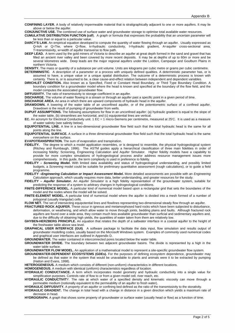
Appendix B

Page 2 of 5

CONFINING LAYER. A body of relatively impermeable material that is stratigraphically adjacent to one or more aquifers. It may lie above or below the aquifer.

CONJUNCTIVE USE. The combined use of surface water and groundwater storage to optimise total available water resources. CUMULATIVE DISTRIBUTION FUNCTION (cdf). A graph or formula that expresses the probability that an uncertain parameter will

be less than or equal to a particular value. DARCY'S LAW. An empirical equation developed to compute the quantity of water flowing through an aquifer. Usually expressed as

Q=kiA or Q=Tiw, where Q=flow, k=hydraulic conductivity, I=hydraulic gradient, A=aquifer cross-sectional area, T=transmissivity, w=width of aquifer transverse to flow path.

DEEP LEAD. A term used by the gold miners of Victoria to describe an aquifer at great depth formed in the sand and gravel that has filled an ancient river valley and been covered by more recent deposits. It may be at depths of up to 60m or more and be several kilometres wide. Deep leads are the major regional aquifers under the Loddon, Campaspe and Goulburn Plains in northern Victoria.

DENSITY. The mass or quantity of a substance per unit volume. Units are kilograms per cubic metre or grams per cubic centimetre. DETERMINISTIC. A description of a parameter or a process with uniquely defined qualities. A deterministic parameter has, or is

assumed to have, a unique value or a unique spatial distribution. The outcome of a deterministic process is known with certainty. There is, or is assumed to be, a clear cause-and-effect relation between independent and dependent variables.

DIRICHLET CONDITION. Also known as a Specified, Fixed or Constant Head Boundary, or Third Type Boundary Condition. A boundary condition for a groundwater model where the head is known and specified at the boundary of the flow field, and the model computes the associated groundwater flow.

DIFFUSIVITY. The ratio of transmissivity to storage coefficient in an aquifer. DISCHARGE. The volume of water flowing in a stream or through an aquifer past a specific point in a given period of time. DISCHARGE AREA. An area in which there are upward components of hydraulic head in the aquifer. DRAWDOWN. A lowering of the water table of an unconfined aquifer, or of the potentiometric surface of a confined aquifer.

Drawdown is the result of pumping of groundwater from wells. DUPUIT ASSUMPTIONS. The following assumptions for flow in an unconfined aquifer: (a) hydraulic gradient is equal to the slope of

the water table, (b) streamlines are horizontal, and (c) equipotential lines are vertical. EC. An acronym for Electrical Conductivity unit. 1 EC = 1 micro-Siemens per centimetre, measured at 25'C. It is used as a measure

of water salinity (see salinity below). EQUIPOTENTIAL LINE. A line in a two-dimensional groundwater flow field such that the total hydraulic head is the same for all

points along the line. EQUIPOTENTIAL SURFACE. A surface in a three dimensional groundwater flow field such that the total hydraulic head is the same

everywhere on the surface. EVAPOTRANSPIRATION. The sum of evaporation and transpiration. FIDELITY. The degree to which a model application resembles, or is designed to resemble, the physical hydrogeological system

(Ritchey and Rumbaugh, 1996). The ASTM guides apply a hierarchical classification of three main fidelities in order of increasing fidelity: Screening, Engineering Calculation and Aquifer Simulator. Higher fidelity models have a capability to provide for more complex simulations of hydrogeological process and/or address resource management issues more comprehensively. In this guide, the term complexity is used in preference to fidelity.

FIDELITY – Screening Model. With limited data availability and status of hydrogeological understanding, and possibly limited budgets, a Screening model could be suitable for preliminary quantitative assessment (rough calculations), or to guide a field programme.

FIDELITY –Engineering Calculation or Impact Assessment Model. More detailed assessments are possible with an Engineering Calculation approach, which usually requires more data, better understanding, and greater resources for the study.

FIDELITY – Aquifer Simulator. An Aquifer Simulator is a high fidelity representation of the groundwater system, suitable for predicting the response of a system to arbitrary changes in hydrogeological conditions.

FINITE-DIFFERENCE MODEL. A particular kind of numerical model based upon a rectangular grid that sets the boundaries of the model and the nodes where the model will be solved.

FINITE-ELEMENT MODEL. A particular kind of numerical model where the aquifer is divided into a mesh formed of a number of polygonal (usually triangular) cells.

FLOW NET. The set of intersecting equipotential lines and flowlines representing two-dimensional steady flow through an aquifer. FRACTURED ROCK AQUIFER. These occur in igneous and metamorphosed hard rocks which have been subjected to disturbance,

deformation, or weathering, and which allow water to move through joints, bedding plains and faults. Although fractured rock aquifers are found over a wide area, they contain much less available groundwater than surficial and sedimentary aquifers and, due to the difficulty of obtaining high yields, the quantities of water taken from them are relatively low.

GHYBEN-HERZBERG PRINCIPLE. An equation that relates the depth of a saltwater interface in a coastal aquifer to the height of the freshwater table above sea level.

GRAPHICAL USER INTERFACE (GUI). A software package to facilitate the data input, flow simulation and results output of groundwater modelling codes, usually based on the Microsoft Windows system. Examples of commonly used numerical codes and graphical user interfaces are outlined in Appendix D.

GROUNDWATER. The water contained in interconnected pores located below the water table. GROUNDWATER DIVIDE. The boundary between two adjacent groundwater basins. The divide is represented by a high in the

water table surface. GROUNDWATER FLOW MODEL. An application of a mathematical model to represent a site-specific groundwater flow system. GROUNDWATER-DEPENDENT ECOSYSTEMS (GDEs). For the purposes of defining ecosystem dependence, groundwater may

be defined as that water in the system that would be unavailable to plants and animals were it to be extracted by pumping (Hatton and Evans, 1998).

HETEROGENEOUS. A medium which consists of different (non-uniform) characteristics in different locations. HOMOGENEOUS. A medium with identical (uniform) characteristics regardless of location. HYDRAULIC CONDUCTANCE. A term which incorporates model geometry and hydraulic conductivity into a single value for

simplification purposes. Controls rate of flow to or from a given model cell, river reach, etc. HYDRAULIC CONDUCTIVITY. The rate at which water of a specified density and kinematic viscosity can move through a

permeable medium (notionally equivalent to the permeability of an aquifer to fresh water). HYDRAULIC DIFFUSIVITY. A property of an aquifer or confining bed defined as the ratio of the transmissivity to the storativity. HYDRAULIC GRADIENT. The change in total head with a change in distance in a given direction which yields a maximum rate of

decrease in head. HYDROGRAPH. A graph that shows some property of groundwater or surface water (usually head or flow) as a function of time.

Appendix B

Page 3 of 5

HYDROLOGIC CONDITIONS. A set of groundwater inflows, outflows, boundary conditions and hydraulic properties that causes potentiometric heads to adopt a distinct pattern.

HYDROLOGIC CYCLE. The circulation of water from the oceans through the atmosphere to the land and ultimately back to the ocean.

HYDROLOGIC EQUATION. An expression of the law of mass conservation for purposes of water budgets. It may be stated as inflow equals outflow plus or minus changes in storage.

IMPERMEABLE LAYERS. Layers of rock which do not allow water to pass through them. INFILTRATION. The flow of water downward from the land surface into and through the upper soil layers. INFILTRATION CAPACITY. The maximum rate at which infiltration can occur under specific conditions of soil moisture. For a given

soil, the infiltration capacity is a function of the water content. INTERFLOW. The lateral movement of water in the unsaturated zone during and immediately after a precipitation event. The water

moving as interflow discharges directly into a stream or lake. ISOTROPY. The condition in which hydraulic properties of the aquifer are equal in all directions. KARST. The type of geologic terrain underlain by carbonate rocks where significant solution of the rock has occurred due to the

flowing groundwater. Karst topography is frequently characterised by sinkholes, caves, and underground drainage. LOCAL GROUNDWATER SYSTEM. Aquifers which respond rapidly to recharge due to a shallow watertable and/or close proximity

of the recharge and discharge sites. These types of flow systems occur almost exclusively in unconfined aquifers. LEAKANCE. Controls vertical flow in a model between cells in adjacent layers. Equivalent to effective vertical hydraulic conductivity

divided by the vertical distance between layer midpoints. LEAKY CONFINING LAYER. A low-permeability layer that can transmit water at sufficient rates to furnish some recharge to a well

pumping from an under-lying aquifer. Also known as an aquitard. LINEAMENT. A regional topographic feature of regional extent that is believed to reflect crustal structure. LYSIMETER. A field device containing a soil column and vegetation; used for measuring evapotranspiration. MEGALITRE (ML). one million litres. MANNING’s EQUATION. An equation that can be used to compute the average velocity of flow in an open channel. MODEL APPLICATION. Refer to Model, Groundwater. MODEL CALIBRATION. The process by which the independent variables (parameters) of a numerical model are adjusted, within

realistic limits, to produce the best match between simulated and observed data (usually water-level values). This process involves refining the model representation of the hydrogeologic framework, hydraulic properties, and boundary conditions to achieve the desired degree of correspondence between the model simulations and observations of the groundwater flow system.

MODEL, conceptual. A simplified and idealised representation (usually graphical) of the physical hydrogeologic setting and our hydrogeological understanding of the essential flow processes of the system. This includes the identification and description of the geologic and hydrologic framework, media type, hydraulic properties, sources and sinks, and important aquifer flow and surface-groundwater interaction processes.

MODEL, groundwater. An application of a mathematical model to represent a site-specific groundwater flow system. A groundwater model provides a scientific means to synthesise the available data into a numerical characterisation of a groundwater system. The model represents the groundwater system to an adequate level of detail, and provides a predictive tool to quantify the effects on the system of specified hydrological stresses.

MODEL - mathematical model. A mathematical model is a set of equations, which, subject to certain assumptions, quantifies the physical processes active in the aquifer. While the model itself obviously lacks the detailed reality of the groundwater system, the behaviour of a valid model approximates that of the aquifer.

MODEL - analytical model. Refer to Analytical Model MODEL - numerical model. Refer to Numerical Model. MONTE CARLO ANALYSIS. A set of model simulations for alternative model realisations, on the assumption that aspects of the

model are stochastic. A realisation is one of many possible valid descriptions of a model in terms of its aquifer parameters, boundary conditions or stresses.

MOUND SPRINGS. These occur in the southwestern and western margins of the Great Artesian Basin. When the water comes to the surface in these arid environments, minerals are precipitated around the spring by evaporative concentration and cooling. The springs are sites of rich endemic flora and fauna. They have long been important to the Aboriginal people and to the pastoral industry.

NEUMANN CONDITION. Also called a constant flux boundary. The boundary condition for a groundwater flow model where a flux across the boundary of the flow region is known and specified, and the model computes the associated aquifer head.

NON-UNIQUENESS. The principle that many different possible sets of model inputs can produce nearly identical computed aquifer head distributions for any given model (see heuristic representation given in Appendix A and Section 3 - Ritchey and Rumbaugh, 1996).

NUMERICAL MODEL. A model of groundwater flow in which the aquifer is described by numerical equations, with specified values for boundary conditions, that are usually solved on a digital computer. In this approach, the continuous differential terms in the governing hydraulic flow equation are replaced by finite quantities. The computational power of the computer is used to solve the resulting algebraic equations by matrix arithmetic. In this way, problems with complex geometry, dynamic response effects and spatial and temporal variability may be solved accurately. This approach must be used in cases where the essential aquifer features form a complex system, and where surface-groundwater interaction is an important component (ie. high complexity models).

OBSERVATION WELL. A non-pumping well used to observe the elevation of the water table or the potentiometric surface. An observation well is generally of larger diameter than a piezometer and typically is screened or slotted throughout the thickness of the aquifer.

PERMEABLE STRATA. Layers of rock through which water can pass. PACKER TEST. An aquifer test performed in an open borehole; the segment of the borehole to be tested is sealed off from the rest

of the borehole by inflating seals, called packers, both above and below the segment. PARSIMONY. The parsimony principle implies that a conceptual model has been simplified as much as possible, yet it retains

enough complexity so that it adequately represents the physical system and its behaviour. PIEZOMETER. A non-pumping well, generally of small diameter, that is used to measure the elevation of the water table or

potentiometric surface. A piezometer generally has a short well screen through which water can enter. POROSITY. The ratio of the volume of void spaces in a rock or sediment to the total volume of the rock or sediment. POROSITY, EFFECTIVE. The volume of the inter-connected void spaces through which water or other fluids can travel in a rock or

sediment divided by the total volume of the rock or sediment. POROSITY, PRIMARY. The porosity that represents the original pore openings when a rock or sediment formed.

Appendix B

Page 4 of 5

POROSITY, SECONDARY. The porosity that has been caused by fractures or weathering in a rock or sediment after it has been formed.

POST-AUDIT. Comparison of model predictions with what actually happened. POTENTIOMETRIC SURFACE. A surface that represents the level to which water will rise in tightly cased wells. The water table is a

particular potentiometric surface of an unconfined aquifer (see SATURATED ZONE). PROBABILITY DISTRIBUTION FUNCTION (pdf). A graph or formula which expresses the probability that an uncertain parameter

will have a particular value. PUMPING TEST. Also known as an aquifer test. A test made by pumping a well for a period of time at a measured rate and

observing the change in hydraulic head in the aquifer. A pumping test may be used to determine the capacity of the well and the hydraulic characteristics of the aquifer.

RECHARGE. The process which replenishes groundwater, usually by rainfall infiltrating from the ground surface to the watertable and by river water entering the watertable or exposed aquifers. The addition of water to an aquifer.

RECHARGE BOUNDARY. An aquifer system boundary that adds water to the aquifer. Streams and lakes are typically recharge boundaries.

REGIONAL GROUNDWATER SYSTEMS. Extensive aquifers which take longer than local systems to respond to increased groundwater recharge because their recharge and discharge sites are separated by large distances (>10 km), and/or they have a deep water table. Unconfined aquifers with deep water tables that are part of regional flow systems may become, in effect, local flow systems if there is sufficient recharge to cause the water table to rise close to the surface (<5m).

REGOLITH. The fragmented and unconsolidated rock material that forms the surface of the land and overlies the bedrock. RESIDUAL. The difference between the computed and observed value of a variable at a specific time and location. ROCK, IGNEOUS. A rock formed by the cooling and crystallisation of a molten rock mass called magma. ROCK, METAMORPHIC. A rock formed by the application of heat and pressure to preexisting rocks. ROCK, SEDIMENTARY. A layered rock formed from the consolidation of sediment. Includes clastic rocks (such as sandstone),

rocks formed by chemical precipitation in water (such as limestone), or rocks formed from organic material (such as coal). ROCK, VOLCANIC. An igneous rock formed when molten rock called lava cools on the earth's surface. SALINITY. The concentration of sodium chloride or dissolved salts in water, usually expressed in EC units or milligrams of total

dissolved solids per litre (mg/L TDS). The conversion factor of 0.6 mg/L TDS = 1 EC unit is commonly used as an approximation.

SALINISATION. The accumulation of salts via the actions of water in the soil to a level that causes degradation of the soil. SATURATED ZONE. The zone in which the voids in the rock or soil are filled with water at a pressure greater than atmospheric. The

water table is the top of the saturated zone in an unconfined aquifer. SEDIMENTARY AQUIFERS. These occur in consolidated sediments such as porous sandstones and conglomerates, in which water

is stored in the intergrannular pores, and limestone, in which water is stored in solution cavities and joints. These aquifers are generally located in sedimentary basins that are continuous over large areas and may be tens or hundreds of metres thick. In terms of quantity, they contain the largest groundwater resources.

SEEPAGE VELOCITY. Also known as pore water velocity. The rate of movement of fluid particles through porous media along a line from one point to another.

SENSITIVITY ANALYSIS. The measurement of the uncertainty in a calibrated model as a function of uncertainty in estimates of aquifer parameters and boundary conditions.

SIMULATION. One complete execution of a groundwater modelling program, including input and output. SIMPLICITY. The simplicity (or parsimony) principle implies that a conceptual model has been simplified as much as possible, yet it

retains enough complexity so that it adequately represents the physical system and its behaviour. SPECIFIC CAPACITY. The ratio of the rate of discharge of water from the well to the drawdown of the water level in the well.

Specific capacity should be described on the basis of the number of hours of pumping prior to the time the drawdown measurement is made. It will generally decrease with time as the drawdown increases.

SPECIFIC DISCHARGE. Also known as Darcian flow velocity. An apparent velocity calculated from Darcy's law; represents the flow rate at which water would flow in an aquifer if the aquifer were an open conduit.

SPECIFIC RETENTION. The ratio of the volume of water the rock or sediment will retain against the pull of gravity to the total volume of the rock or sediment.

SPECIFIC STORAGE. The amount of water per unit volume of a saturated formation that is expelled from storage due to compression of the mineral skeleton and the pore water.

SPECIFIC YIELD. The ratio of the volume of water that a given mass of saturated soil or rock will yield by gravity to the volume of that mass.

STOCHASTIC. A description of a parameter or a process with random qualities. A stochastic parameter has a range of possible values, each with a defined probability. The outcome of a stochastic process is not known with certainty.

STORAGE COEFFICIENT (STORATIVITY). The volume of water that a conductive unit will expel from storage per unit surface area per unit change in head. In a confined aquifer, it is computed as the product of specific storage and aquifer thickness. In an unconfined aquifer, it is equal to specific yield.

STREAMLINE. A line (commonly transverse to groundwater level contours) that represents the flow path for a particle of water. SUB-ARTESIAN. Groundwater that does not rise above the surface of the ground when accessed by a bore and must be pumped to

the surface. SURFICIAL (SUPERFICIAL) AQUIFERS. These occur in alluvial sediments in river valleys, deltas, basins and coastal plains, in lake

or lacustrine sediments, and in aeolian or wind-formed deposits. They are essentially unconsolidated day, silt, sand, gravel, and limestone formations, mainly of Quaternary age (under 1.8 million years). These deposits are easily exploited and are the major sources of freshwater groundwater when associated with larger river systems.

THEIS EQUATION. An equation for the unsteady flow of groundwater in a fully confined aquifer to a pumping well. TOPOGRAPHIC DIVIDE. The boundary between adjacent surface water boundaries. It is represented by a topographically high

area. TORTUOSITY. The actual length of a groundwater flow path, which is sinuous in form, divided by the straight-line distance between

the ends of the flow path. TOTAL DISSOLVED SOLIDS (TDS). A measure of the salinity of water, usually expressed in milligrams per litre (mg/L). Sometimes

TDS is referred to as total dissolved salts, or as TSS, total soluble salts. See also EC. TRANSMISSIVITY. The rate at which water is transmitted through a unit width of aquifer of confining bed under a unit hydraulic

gradient. The product of saturated thickness and hydraulic conductivity. TRANSPIRATION. The loss of water vapour from plants. UNCERTAINTY ANALYSIS. The quantification of uncertainty in model results due to incomplete knowledge of model aquifer

parameters, boundary conditions or stresses.

Appendix B

Page 5 of 5

UNCONFINED AQUIFER. An aquifer that contains the watertable and is normally exposed to the surface. Occasionally there may be a layer overlying this type of aquifer protecting it from the surface.

UNSATURATED ZONE. Also known as the zone of aeration and the vadose zone. The zone between the land surface and the water table. It includes the root zone, intermediate zone, and capillary fringe. The pore spaces contain water at less than atmospheric pressure, as well as air and other gases. Saturated bodies, such as perched groundwater, may exist in the unsaturated zone.

VADOSE ZONE. See UNSATURATED ZONE. VALIDATION. See VERIFICATION. VERIFICATION. A test of the integrity of a model by checking if its predictions reasonably match the observations of a reserved data

set, deliberately excluded from consideration during calibration. VISCOSITY. The property of fluid describing its resistance to flow. Units of viscosity are Newton-seconds per metre squared or

Pascal-seconds. Viscosity is also known as dynamic viscosity. WATER BUDGET. An evaluation of all the sources of supply and the corresponding discharges with respect to an aquifer or a

drainage basin. WATER TABLE. The upper level of the unconfined groundwater, where the water pressure is equal to that of the atmosphere and

below which the soils or rocks are saturated. It is the location where the sub-surface becomes fully saturated with groundwater, the level at which water stands in wells that penetrate the water body. Above the water table, the sub-surface is only partially saturated (often called the unsaturated zone). The water table can be measured by installing shallow wells extending just into the zone of saturation and then measuring the water level in those wells.

WELL DEVELOPMENT. The process whereby a well is pumped or surged to remove any fine material that may be blocking the well screen or the aquifer outside the well screen.

WELL EFFICIENCY. The ratio of idealised drawdown in the well, where there are no losses resulting from well design and construction factors, to actual measured drawdown in the well.

WELL, FULLY PENETRATING. A well drilled to the bottom of an aquifer, constructed in such a way that it withdraws water from the entire thickness of the aquifer.

WELL, PARTIALLY PENETRATING. A well constructed in such a way that it draws water directly from a fractional part of the total thickness of the aquifer. The fractional part may be located at the top or bottom or anywhere in between in the aquifer.

WELL SCREEN. A tubular device with either slots, holes, gauze, or continuous-wire wrap; used at the end of a well casing to complete a well. The water enters the well through the well screen.

YIELD, SAFE. The amount of naturally occurring groundwater that can be economically and legally withdrawn from an aquifer on a sustained basis without impairing the native groundwater quality or creating an undesirable effect such as environmental damage. It cannot exceed the increase in recharge or leakage from adjacent strata plus the reduction in discharge that is due to the decline in head caused by pumping.

YIELD, SUSTAINABLE. An accepted working definition of sustainable yield in NSW is (Kalaitzis et al, 1999): “Sustainable yield is that proportion of the long term average annual recharge which can be extracted each year without causing unacceptable impacts on groundwater users or the environment”. The default proportion has been set at 70%, but this figure can be adjusted locally by a Groundwater Management Committee.

Appendix C

Template for a Brief for a

Groundwater Flow Modelling Study

Appendix C

Page 1 of 2

Appendix C Template for a Brief for a Groundwater Flow Modelling Study

1. Preamble Brief description of aquifer system and degree of utilisation of water resources, major water uses/users. 2. Purpose Outline the purpose of the study in specific terms and in relation to the particular resource management issues of current concern that the model will be used to address. Substantial stakeholder involvement is required for this task. 3. Objectives Outline the specific and measurable objectives of the study (ie. the outcomes required, or the answers being sought). Substantial stakeholder involvement is required for this task. 4. Model Complexity Suggest a minimum model complexity (refer to definition given in the guideline or the glossary of the technical guideline), and indicate the staged development of complexity improvements (if applicable). 5. Study Resources Indicate in general or specific terms the resources available or expected to be applied to the study (broad budget, schedule, staged model development, eventual ownership and use of model). 6. Data Available Outline the data available to be used in the initial hydrogeological interpretation, development of the conceptual model and in model calibration, with specific detail to cover the following key components, noting the periods of record available, the general data quality and any known data quality problems: • Topography (maps and scale) • Climate (rainfall, evaporation) • Hydrology (surface drainage network, flow data) • Hydrogeology (maps, reports, bore networks, groundwater levels, surface-groundwater interaction) • Pumping (surface water, groundwater, licensed amounts, actual records, format of data) • Water quality (surface water, groundwater) 7. Literature Review Listing List all known reports and published documents/maps, papers etc., dealing with the area. 8. Calibration and Prediction Indication of the preferred timeframe for model calibration and verification, the suggested minimum accuracy requirement, and the suggested method of sensitivity and/or uncertainty assessment. 9. Prediction Scenarios Outline the following for the initial set of prediction scenarios (limited number): • number of prediction simulations required (a small number for initial model development) and the

types of prediction runs required (eg. pumping rate ranges and timing, climatic variations, etc.) • prediction run timeframe and hydrological data set to be used (eg. a repeat of the historical record,

or synthetic data set) • type of sensitivity and/or uncertainty assessment, especially for prediction outside the range of

hydrological stresses and aquifer water level responses considered during calibration periods. It should be possible for subsequent prediction run programmes to be undertaken on a lump sum basis per scenario.

Appendix C

Page 2 of 2

10. Project Management Outline of the study team and method of review of technical aspects and contract administration, including: • Project Manager and/or Technical Steering Group details • Reporting requirements (timing, format and number of copies, period for review and revision of draft

technical reports, frequency of technical and project management progress reporting) • Likely model reviewer and method of review (provision of model data set and software requirements) • Expected meetings to discuss reviews (technical or administrative), or to present results to

nominated audiences. 11. Information to be provided by Tenderer: • Commitment from Tenderer to utilise nominated staff on the project team, with written approval

required before alternatives may be used • Study team structure details, with brief biographies or full CVs provided (as required), and an

indication of methods for in-house review • General description of the site/catchment in hydrological and hydrogeological terms • Brief description of the main critical elements and features of the conceptual model (noting that the

development of a valid and comprehensive conceptual model forms part of the actual study, as it requires specialist skills, substantial data analysis, and the application of reasoned judgement, which is not a cost-free service)

• Schedule of fee rates and expenses, with an estimated budget (possibly indicating an upper limiting fee that may not be exceeded without written authorisation), and a time schedule to complete the scope of work outlined

• Outline of the table of contents for required reports • Proposed presentation of output from the model that is relevant to the particular study. For example,

for a dryland salinity or irrigation seepage study, the depth to groundwater may be important. For abstraction impact assessment (eg. for irrigation, town water supply or dewatering), drawdown or groundwater level results may be important, along with abstraction volumes.

• If the Tenderer is offering specialist services as an independent expert/model reviewer, the following key issues are relevant: - Level of local hydrogeological knowledge (or access to such knowledge) - General experience as a modelling specialist - Experience as a modelling team leader - Numbers of models developed of various degrees of complexity - Expert skills in specific modelling packages (especially the one to be used in the study) and/or

specific model types (eg. finite difference/finite element; 3D/quasi-3D/2D; flow/solute transport/heat/density coupled)

- Experience of modelling a range of hydrological and hydrogeological conditions (eg. arid, tropical, temperate, irrigation, mine dewatering, dryland salinity, complex river-aquifer interaction).

Appendix D

Table 1 – Summary of 3D Groundwater Flow Modelling Codes Table 2 – Summary of MODFLOW Graphical User Interfaces Table 3 – Minimum Aquifer Parameter Requirements for MODFLOW

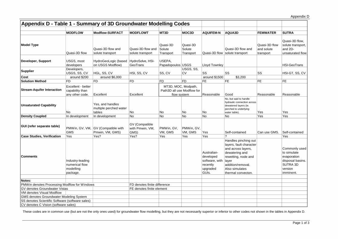
Appendix D

Page 1 of 3

These codes are in common use (but are not the only ones used) for groundwater flow modelling, but they are not necessarily superior or inferior to other codes not shown in the tables in Appendix D.

Appendix D - Table 1 - Summary of 3D Groundwater Modelling Codes

MODFLOW Modflow-SURFACT MODFLOWT MT3D MOC3D AQUIFEM-N AQUA3D FEMWATER SUTRA

Model Type

Quasi-3D flowQuasi-3D flow and solute transport

Quasi-3D flow and solute transport

Quasi-3D Solute Transport

Quasi-3D Solute Transport Quasi-3D flow



Quasi-3D flow, solute transport, and 2D-unsaturated flow

Developer, Support USGS, most developers

HydroGeoLogic (based on USGS Modflow)

HydroSolve, HSI-GeoTrans

USEPA, Papadopoulos USGS Lloyd Townley HSI-GeoTrans

Supplier Developers, USGS, SS, CV HGL, SS, CV HSI, SS, CV SS, CV

USGS, SS, CV SS SS SS HSI-GT, SS, CV

Cost around $200 around $6,000 around $1500 $3,200 Solution Method FD FD FD FD FD FE FE FE FE

Stream-Aquifer InteractionExcellent - better capability than any other code. Excellent Excellent Reasonable Good Reasonable Reasonable

Unsaturated Capability

No

Yes, and handles multiple perched water tables No No No No

No, but said to handle hydraulic connection across dewatered layers (ie. perched to underlying water table). Yes Yes

Density Coupled In development In development No No No No No Yes Yes

GUI (refer separate table)PMWin, GV, VM, GMS

GV (Compatible with Pmwin, VM, GMS)

GV (Compatible with Pmwin, VM, GMS)

PMWin, GV, VM, GMS

PMWin, GV, VM, GMS Yes Self-contained Can use GMS. Self-contained

Case Studies, Verification Yes Yes? Yes? Yes Yes Yes ? Yes

CommentsIndustry-leading numerical flow modelling package.

Australian-developed software, with recently upgraded GUIs.

Handles pinching out layers, fault character and across layers, dewatering and rewetting, node and layer addition/removal. Also simulates thermal convecton.

Commonly used to simulate evaporation disposal basins. SUTRA 3D version imminent.

Notes:PMWin denotes Processing Modflow for Windows FD denotes finite differenceGV denotes Groundwater Vistas FE denotes finite elementVM denotes Visual ModflowGMS denotes Groundwater Modeling SystemSS denotes Scientific Software (software sales)CV denotes C Vision (software sales)

MT3D, MOC, Modpath, Path3D all use Modflow for

flow system

Appendix D

Page 2 of 3

Appendix D - Table 2 - Summary of Modflow Graphical Interfaces Package Groundwater Vistas Modflow-Surfact Processing Modflow Visual Modflow Groundwater Modeling

System Abbreviation GV MS-VMS PMWin VM GMS Approx. Cost $1,400 $6,000 $1,600 $1,600 $3,000 to $6,000 depending on

options Developer, Support ESI HydroGeoLogic Chiang & Kinzelbach Waterloo Hydrogeologic US Dept of Defence, EMSI,

Brigham Young University Supplier ESI, SS, CV ESI, HGL, SS Developer, SS, CV Waterloo Hydrogeologic, SS,

CV SS, CV, EMSI

Unsaturated Capability Yes, with Modflow-Surfact from HydroGeoLogic ($4,000)

Yes (Richard's equation), with air phase flow simulation.

No No No with Modflow package. Yes, in FemWater package.

Density Coupled in development in development PMWin Density Package No Yes, in FemWater package. Fracture Flow No Yes No No No. Solute Transport and Particle Tracking

MT3D, MODPATH MT3D, MODPATH MT3D, MT3DMS, MOC3D, PMPath99

MT3D, ModPath MT3D, ModPath, RT3DMOC3D, SEAM3D

Supports (additional purchase required)

MT3DMS, RT3D, MOC3D, Path3D, ModflowT, Modflow-Surfact

MT3DMS, RT3D, MOC3D, Path3D

MT3DMS, MT3D99, RT3D FemWater, Seep2D, SEAM3D.

Auto Calibration Supports Pest, UCODE Supports Pest, UCODE Bundled with Pest (Lite), UCODE Supports WinPest Limited. Presentation and SURFER Compatibility

Imports and exports SURFER grid and data files. Export DXF, HPGL, BMP. 3D animation with TecPlot.

Imports and exports SURFER grid and data files. Export DXF, HPGL, BMP. 3D animation with TecPlot.

Import SURFER grid, geo-referenced raster graphics. Export SURFER data files, DXF, HPGL, BMP.

Import/export SURFER grid & data files. Export DXF, EMF, ESRI shape file. 3D animation with Visual Groundwater.

GIS capability (Arc/Info, ArcView), import/export DXF (AutoCad or MicroStation).

Telescopic mesh refinement Yes Yes Yes No Yes. On-screen Views Plan and cross-section Plan and cross-section Plan in flow model, plan and cross-

section in particle tracking. Some animation. Velocity vectors.

Plan and cross-section Plan and cross-sections of heads, drawdowns and velocity vectors, and animation.

Parameter sensitivity analysis

automated automated No No Limited.

Current Development Development is ongoing. Notable enhancements in progress includes density coupling.

Yes, to include surface and groundwater modelling, integrated with unsaturated flow capability, and fracture flow (dual porosity and discrete fracture), density coupling, and biodegradation.

Yes , notably to incorporate MODBRANCH stream-aquifer interaction package.

Yes, but usually lags other developers.

Yes. Based on Modflow package, with added interfaces to other models. Matrix calculation capability. Additional modules for 2D and 3D geostatistics, borehole logs, fence diagrams, iso-surfaces, etc.

Comments Excellent model design and editing tools, matrix calculations, scroll bars, excellent help and technical support, linkages with developers of advanced Modflow packages (Surfact and ModflowT), full support of all recently released Modflow packages. Developer active in a range of groundwater software, and runs a consultancy firm in USA.

Outstanding features, but quite expensive. Notable features include unsaturated flow capability (including air phase), stable simulation of dewatering-rewetting processes, including hydraulic connection between perched and underlying water tables, ponding and non-ponding recharge capability, TVD (robust) solute transport solver. Other comments as for GV.

Excellent model design and editing tools, matrix calculations, but no scroll bars, good help and technical support, developer is a lecturer at the University of the Free State, and is active in development and publishing of a range of groundwater software (PMWin version 4 available free from ww.uovs.ac.za/igs/index.htm). Support for all recently released Modflow packages.

No scroll bars, poor help, reported poor performance in technical support, questionable support for STR1 stream package, basic matrix calculator, poor editing capability for individual cells.

Excellent borelog database development and plotting. Solids modelling with strong geostatistics and GIS interaction. Very strong in conceptual model development and translation to Modflow or Femwater databases.

SS denotes Scientific Software (software sales); CV denotes C Vision (Australian software sales);

Appendix D

Page 3 of 3

Appendix D - Table 3 - Minimum Aquifer Parameter Requirements for MODFLOWHorizontal Vertical Vertical Layer Geometry Storage Specific Porosity

Transmissivity Conductivity Conductivity Leakance Top Bottom Coefficient Yield (for particleT Kh Kv Vcont S Sy tracking)

Confined (2D)Steady State X (X) (X) (X)

Transient X (X) (X) (X) X (X)Solute Transport X (X) X X X (X) X

Confined (3D)Steady State X (X) (X) X (X) (X)

Transient X (X) (X) X (X) (X) X (X)Solute Transport X (X) (X) X X X X (X) X

Unconfined (2D)Steady State X X X

Transient (X) X X X XSolute Transport (X) X X X X X

Unconfined+Confined (3D)Steady State (X) X (X) (X) X X

Transient (X) X (X) (X) X X X XSolute Transport (X) X (X) (X) X X X X X

NotesX denotes minimum requirement(X) denotes alternative data requirement

Appendix E

Table E1 – Checklist for Model Appraisal

Appendix E

Page 1 of 2

MODEL APPRAISAL PAGE 1 OF 2

Q. QUESTION Not Applicable

or Unknown

Score 0 Score 1 Score 3 Score 5 Score Max. Score

(0, 3, 5)

COMMENT

1.0 THE REPORT 1.1 Is there a clear statement of project objectives in the

modelling report? Missing Deficient Adequate Very Good

1.2 Is the level of model complexity clear or acknowledged? Missing No Yes 1.3 Is a water or mass balance reported? Missing Deficient Adequate Very Good 1.4 Has the modelling study satisfied project objectives? Missing Deficient Adequate Very Good 1.5 Are the model results of any practical use? No Maybe Yes 2.0 DATA ANALYSIS 2.1 Has hydrogeology data been collected and analysed? Missing Deficient Adequate Very Good 2.2 Are groundwater contours or flow directions presented? Missing Deficient Adequate Very Good 2.3 Have all potential recharge data been collected and

analysed? (rainfall, streamflow, irrigation, floods, etc.) Missing Deficient Adequate Very Good

2.4 Have all potential discharge data been collected and analysed? (abstraction, evapotranspiration, drainage, springflow, etc.)

Missing Deficient Adequate Very Good

2.5 Have the recharge and discharge datasets been analysed for their groundwater response?


2.6 Are groundwater hydrographs used for calibration? No Maybe Yes 2.7 Have consistent data units and standard geometrical

datums been used? No Yes

3.0 CONCEPTUALISATION 3.1 Is the conceptual model consistent with project objectives

and the required model complexity? Unknown No Maybe Yes

3.2 Is there a clear description of the conceptual model? Missing Deficient Adequate Very Good 3.3 Is there a graphical representation of the modeller’s

conceptualisation? Missing Deficient Adequate Very Good

3.4 Is the conceptual model unnecessarily simple or unnecessarily complex?

Yes No

4.0 MODEL DESIGN 4.1 Is the spatial extent of the model appropriate? No Maybe Yes 4.2 Are the applied boundary conditions plausible and

unrestrictive? Missing Deficient Adequate Very Good

4.3 Is the software appropriate for the objectives of the study? No Maybe Yes

Appendix E

Page 2 of 2

MODEL APPRAISAL PAGE 2 OF 2


or Unknown


(0, 3, 5)

COMMENT

5.0 CALIBRATION 5.1 Is there sufficient evidence provided for model calibration? Missing Deficient Adequate Very Good 5.2 Is the model sufficiently calibrated against spatial

observations? Missing Deficient Adequate Very Good

5.3 Is the model sufficiently calibrated against temporal observations?


5.4 Are calibrated parameter distributions and ranges plausible?

Missing No Maybe Yes

5.5 Does the calibration statistic satisfy agreed performance criteria?


5.6 Are there good reasons for not meeting agreed performance criteria?


6.0 VERIFICATION 6.1 Is there sufficient evidence provided for model

verification? Missing Deficient Adequate Very Good

6.2 Does the reserved dataset include stresses consistent with the prediction scenarios?

Unknown No Maybe Yes

6.3 Are there good reasons for an unsatisfactory verification? Missing Deficient Adequate Very Good 7.0 PREDICTION 7.1 Have multiple scenarios been run for climate variability? Missing Deficient Adequate Very Good 7.2 Have multiple scenarios been run for operational

/management alternatives? Missing Deficient Adequate Very Good

7.3 Is the time horizon for prediction comparable with the length of the calibration / verification period?


7.4 Are the model predictions plausible? No Maybe Yes 8.0 SENSITIVITY ANALYSIS 8.1 Is the sensitivity analysis sufficiently intensive for key

parameters? Missing Deficient Adequate Very Good

8.2 Are sensitivity results used to qualify the reliability of model calibration?


8.3 Are sensitivity results used to qualify the accuracy of model prediction?


9.0 UNCERTAINTY ANALYSIS 9.1 If required by the project brief, is uncertainty quantified in

any way? Missing No Maybe Yes

TOTAL SCORE PERFORMANCE: %

Appendix F

Table F1 – Checklist for Peer Review of High Complexity Models

Appendix F

Page 1 of 9

MODEL REVIEW: 1. THE REPORT


or Unknown


(0, 3, 5)

COMMENT

1.1 Is a report provided? No Yes 1.2 Are relevant prior or companion reports provided or

accessible? No Yes

1.3 Is it clear which person(s) did the modelling? No Yes 1.4 Is the report well structured? Deficient Adequate Very Good 1.5 Is the report presentation of acceptable quality? Deficient Adequate Very Good 1.6 Is there a clear statement of project objectives? Missing Deficient Adequate Very Good 1.7 Is the level of model complexity clear or acknowledged? Missing No Yes 1.8 Are model parameter distributions disclosed? Missing Deficient Adequate Very Good 1.9 Are model parameter statistics reported (median, range,

standard deviation)? Missing Deficient Adequate Very Good

1.10 Is it clear how stress datasets have been compiled? Missing Deficient Adequate Very Good 1.11 Would it be possible to re-create the structure of the model

from what is reported? No Maybe Yes

1.12 Is a water or mass balance reported? Missing Deficient Adequate Very Good 1.13 Are recommendations reasonable and supported by

evidence? Missing Deficient Adequate Very Good

1.14 Has the modelling study satisfied project objectives? Missing Deficient Adequate Very Good 1.15 Are the model results of any practical use? No Maybe Yes 1.16 Has the modelling study been cost-effective? No Maybe Yes 1. TOTAL SCORE

Appendix F

Page 2 of 9

MODEL REVIEW: 2. DATA ANALYSIS


or Unknown


(0, 3, 5)

COMMENT

2.1 Have prior investigations been examined and acknowledged?


2.2 Is current knowledge sufficient for a mathematical model? No Maybe Yes 2.3 Is there a cost-effective alternative to modelling which would

satisfy the project objectives? Yes Maybe No

2.4 Has a literature review been completed? Missing Deficient Adequate Very Good 2.5 Has hydrogeology data been collected and analysed? Missing Deficient Adequate Very Good 2.6 Has rainfall data been collected and analysed? Missing Deficient Adequate Very Good 2.7 Has streamflow data been collected and analysed? Missing Deficient Adequate Very Good 2.8 Has flood event data been collected and analysed? Missing Deficient Adequate Very Good 2.9 Has irrigation data been collected and analysed? Missing Deficient Adequate Very Good 2.10 Has groundwater usage data been collected and analysed? Missing Deficient Adequate Very Good 2.11 Has evapotranspiration data been collected and analysed? Missing Deficient Adequate Very Good 2.12 Has drainage data been collected and analysed? Missing Deficient Adequate Very Good 2.13 Has other data been collected and analysed? Missing Deficient Adequate Very Good Other data: 2.14 Have the above stress datasets been analysed for their

groundwater response? Missing Deficient Adequate Very Good

2.15 Is any relevant dataset ignored? Yes Maybe No 2.16 Are residual mass (cumulative deviation) plots prepared for

rainfall / streamflow? Missing Deficient Adequate Very Good

2.17 Is groundwater hydrographic data available? No Maybe Yes 2.18 Are representative hydrographs selected logically? Missing Deficient Adequate Very Good 2.19 Are field hydrographs compared and analysed? Missing Deficient Adequate Very Good 2.20 Is water table / piezometric surface data available? No Maybe Yes 2.21 Are representative contour maps selected logically? Missing Deficient Adequate Very Good 2.22 Is interpolation reliability clear to the reader (posting of

sample points, algorithm)? Missing Deficient Adequate Very Good

2.23 Are data units consistent? No Yes 2.24 Have standard geometrical datums been used? No Maybe Yes 2.25 If groundwater flow is likely to be affected by density, has

allowance been made for the effect in any way? Missing Deficient Adequate Very Good

2. TOTAL SCORE

Appendix F

Page 3 of 9

MODEL REVIEW: 3. CONCEPTUALISATION


or Unknown


(0, 3, 5)

COMMENT

3.1 Is the conceptual model consistent with prior knowledge? Unknown No Maybe Yes 3.2 Is the conceptual model consistent with project budget? Unknown No Maybe Yes 3.3 Is the conceptual model consistent with project objectives

and the required model complexity? Unknown No Maybe Yes

3.4 Is the conceptual model consistent with project deadline? Unknown No Maybe Yes 3.5 Is there a clear description of the conceptual model? Missing Deficient Adequate Very Good 3.6 Is there a graphical representation of the modeller’s

conceptualisation? Missing Deficient Adequate Very Good

3.7 Is the conceptual model unnecessarily simple? Yes No 3.8 Is the conceptual model unnecessarily complex? Yes No 3.9 If any possibly key process is missing, is the justification

adequate? Missing Deficient Adequate Very Good

3.10 Are limitations and uncertainties described? No Maybe Yes 3.11 Has the conceptual model been reviewed independently? Unknown No Maybe Yes 3. TOTAL SCORE

Appendix F

Page 4 of 9

MODEL REVIEW: 4. MODEL DESIGN


or Unknown


(0, 3, 5)

COMMENT

4.1 Is the choice of mathematical model appropriate (analytical / numerical)?

No Maybe Yes

4.2 Is the spatial extent of the model appropriate? No Maybe Yes 4.3 Is the spatial discretisation scale appropriate? Missing No Maybe Yes 4.4 Is the number of model layers justified? Missing No Maybe Yes 4.5 Is steady state simulated? Missing Deficient Adequate Very Good 4.6 Is transient behaviour simulated? Missing Deficient Adequate Very Good 4.7 Is the stress period reasonable? Missing No Maybe Yes 4.8 Is the number of time steps per stress period justified? Missing Deficient Adequate Very Good 4.9 Are the applied boundary conditions plausible and

unrestrictive? Missing Deficient Adequate Very Good

4.10 Are boundary condition locations consistent with the model grid configuration?


4.11 Are the initial conditions defensible? Missing Deficient Adequate Very Good 4.12 Is it clear what software has been selected? Missing No Maybe Yes 4.13 Is the software appropriate for the objectives of the study? No Maybe Yes 4.14 Is the software reputable? No Maybe Yes 4.15 Is the software in common use and accessible to reviewers? No Maybe Yes 4.16 How detailed is the rainfall recharge algorithm? Missing Deficient Adequate Very Good 4. TOTAL SCORE

Appendix F

Page 5 of 9

MODEL REVIEW: 5. CALIBRATION


or Unknown


(0, 3, 5)

COMMENT

5.1 Is sufficient data available for spatial calibration? No Maybe Yes 5.2 Is sufficient data available for temporal calibration? No Maybe Yes 5.3 Does the model claim to be adequately calibrated for the

purpose of the study? Missing No Maybe Yes

5.4 Are calibration difficulties acknowledged? Missing Deficient Adequate Very Good 5.5 Is it clear whether calibration is automated or trial-and-error? Missing No Yes Automation software: 5.6 Is there sufficient evidence provided for model calibration? Missing Deficient Adequate Very Good 5.7 Is the model sufficiently calibrated against spatial

observations? Missing Deficient Adequate Very Good

5.8 Is the model sufficiently calibrated against temporal observations?


5.9 Are parts of the model well calibrated? Unknown No Maybe Yes 5.10 Are parts of the model poorly calibrated? Unknown Yes Maybe No 5.11 Is the model calibrated to data from different hydrological

regimes? Unknown No Maybe Yes

5.12 Are calibrated parameter distributions and ranges plausible? Missing No Maybe Yes 5.13 Is a calibration statistic reported? Missing No Yes 5.14 Does the calibration statistic satisfy agreed performance

criteria? Missing Deficient Adequate Very Good

5.15 Are there good reasons for not meeting agreed performance criteria?


5. TOTAL SCORE

Appendix F

Page 6 of 9

MODEL REVIEW: 6. VERIFICATION


or Unknown


(0, 3, 5)

COMMENT

6.1 Has some data been reserved for a verification exercise? Missing No Maybe Yes 6.2 Is the reserved data set an extension of the time period? Missing No Maybe Yes 6.3 Is the reserved dataset a suite of hydrographs not on the

representative list? Missing No Maybe Yes

6.4 Is the volume of reserved data sufficient to establish verification?


6.5 Does the model claim to be verified? Missing No Maybe Yes 6.6 Is there sufficient evidence provided for model verification? Missing Deficient Adequate Very Good 6.7 Are parts of the model well verified? Unknown No Maybe Yes 6.8 Are parts of the model poorly verified? Unknown Yes Maybe No 6.9 Is the reserved dataset from a different hydrological regime? Unknown No Maybe Yes 6.10 Does the reserved dataset include stresses consistent with

the prediction scenarios? Unknown No Maybe Yes

6.11 Are there good reasons for an unsatisfactory verification? Missing Deficient Adequate Very Good 6. TOTAL SCORE

Appendix F

Page 7 of 9

MODEL REVIEW: 7. PREDICTION


or Unknown


(0, 3, 5)

COMMENT

7.1 Is prediction made for steady state conditions? Missing No Maybe Yes 7.2 Is prediction made for transient conditions? Missing No Maybe Yes 7.3 Are the assumed stresses reasonable? Missing Deficient Adequate Very Good 7.4 Is the time horizon for prediction comparable with the length

of the calibration / verification period? Missing No Maybe Yes

7.5 Have multiple scenarios been run for climate variability? Missing Deficient Adequate Very Good 7.6 Have multiple scenarios been run for operational

alternatives? Missing Deficient Adequate Very Good

7.7 Are model predictions made at scales consistent with model space and time scales?


7.8 Are the model predictions plausible? No Maybe Yes 7.9 Are model predictions likely to be impacted by constraining

boundary conditions? Unknown Yes Maybe No

7.10 If boundary conditions affect the predictions, are the predictions defensible?


7. TOTAL SCORE

Appendix F

Page 8 of 9

MODEL REVIEW: 8. SENSITIVITY ANALYSIS


or Unknown


(0, 3, 5)

COMMENT

8.1 Is there discussion of qualitative sensitivities found during calibration?


8.2 Has a post-calibration sensitivity analysis been performed? Missing Deficient Adequate Very Good 8.3 Is the sensitivity analysis sufficiently intensive for key

parameters? Missing Deficient Adequate Very Good

8.4 Is there a graphical presentation of sensitivity behaviour? Missing Deficient Adequate Very Good 8.5 Are sensitivities classified as Type I to Type IV? Missing No Yes See Guidelines Section 5.2 8.6 Has a Type IV sensitivity been recognised? Missing Yes Maybe No See Guidelines Section 5.2 8.7 Is there a list of ranked sensitivity coefficients? Missing Deficient Adequate Very Good 8.8 Are sensitivity results used to qualify the reliability of model

calibration? Missing Deficient Adequate Very Good

8.9 Are sensitivity results used to qualify the accuracy of model prediction?


8. TOTAL SCORE

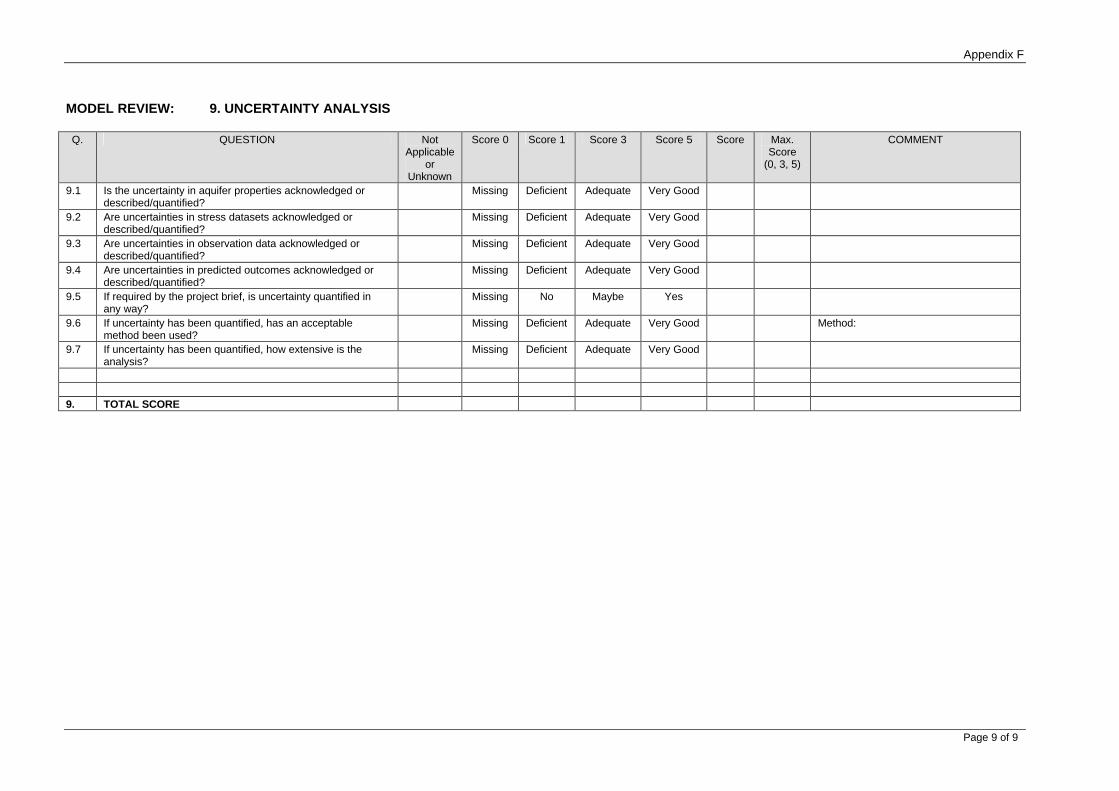
Appendix F

Page 9 of 9

MODEL REVIEW: 9. UNCERTAINTY ANALYSIS


or Unknown


(0, 3, 5)

COMMENT

9.1 Is the uncertainty in aquifer properties acknowledged or described/quantified?


9.2 Are uncertainties in stress datasets acknowledged or described/quantified?


9.3 Are uncertainties in observation data acknowledged or described/quantified?


9.4 Are uncertainties in predicted outcomes acknowledged or described/quantified?


9.5 If required by the project brief, is uncertainty quantified in any way?


9.6 If uncertainty has been quantified, has an acceptable method been used?

Missing Deficient Adequate Very Good Method:

9.7 If uncertainty has been quantified, how extensive is the analysis?


9. TOTAL SCORE

Appendix G

Table G1 – Checklist for Model Compliance Assessment

Appendix G

Page 1 of 1

CHECKLIST FOR MODEL COMPLIANCE ASSESSMENT PAGE 1 OF 1

Q. QUESTION PASS FAIL IF ‘PASS’: COMMENT IF ‘FAIL’: CORRECTIVE ACTION REQUIRED

1 Are the objectives of the modelling study stated clearly?

2 Are the objectives satisfied?

3 Is the conceptual model consistent with project objectives and agreed model complexity?

4 Is the conceptualisation based on the full data set and a competent analysis of available data, and presented clearly?

5 Has the conceptualisation been developed, endorsed or reviewed by a competent hydrogeologist (and revised if necessary)?

6 Does model design/implementation conform with best practice?

7 Is model calibration satisfactory?

8 Are calibrated aquifer property values plausible?

9 Does model prediction/application conform with best practice?

10 Is there an excessive number of “Missing” or “Deficient” task performances marked on the Model Appraisal or Model Review Checklists?

Appendix H

Summary of Recommended Guidelines

Appendix H

Page 1 of 4


No. Guideline 1

(a)

(b)

(c)

(d)

(e)

(f)

(g) (h)

(i)

Summary of recommended guidelines for achieving modelling study best practice Clearly state, at the outset, the model study objectives and the model complexity required (Section 2.1). Adopt a level of complexity that is high enough to meet the objective, but low enough to allow conservatism where needed (Section 2.4). Develop a conceptual model that is consistent with available information and the project objective (Section 2.4). Document the assumptions involved. If possible, a suitably experienced hydrogeologist/modeller should undertake a site visit at the conceptualisation stage. Address the non-uniqueness problem by using measured hydraulic properties, and calibrating to data sets collected from multiple distinct hydrologic conditions (Section 3.2). Perform an assessment of the model uncertainty by undertaking application verification, and sensitivity or uncertainty analysis of calibration and prediction simulations (Section 5). Provide adequate documentation of the model development and predictions (Section 6). Undertake peer review of the model at various stages throughout its development, and to a level of detail appropriate for the model study scope and objectives (Section 7). Maintain effective communication between all parties involved in the modelling study through regular progress reporting (technical issues and project management) and review.

2.1 (a)

(b)

(c)

(d)

Recommended guideline for defining modelling study objectives, complexity and resources: The modelling study objective and purpose must be clearly stated in specific and measurable terms, along with the resource management objectives that the model will be required to address. The overall management constraints should be outlined in terms of budget, schedule, staged development and long term maintenance, and eventual ownership and use of the model. The model complexity must be assessed and defined to suit the study purpose, objectives and resources available for each model study The model complexity assessment must involve negotiation between a client/end-user and the modelling team, including the model reviewer, and relevant government agency representatives.

2.2 (a)

(b)

(c)

Recommended guidelines for data collation and initial hydrogeological interpretation: The available reports on the study area should be collated and listed by the project manager and a broad description of the essential features of the hydrogeological system outlined in the study brief. The brief should also identify and list data sources, types and quality, and known issues that may affect the selection of an appropriate model complexity and the setting of calibration accuracy targets. The modelling study should be initiated with a literature review and data analysis in order to develop an understanding of the important aspects of the physical system, data reliability, and of the hydrological processes that control or impact the groundwater flow system. The data analysis should identify data gaps that may affect the model development, and recommend field programmes necessary for additional data acquisition. The initial literature review and data analysis step needs to be adequately resourced for the purposes of the modelling study. The available data to be used in model input or in calibration assessment should be collated into a database (spreadsheet format as a minimum).

2.3 (a) (b)

(c) (d) (e) (f)

Recommended guidelines for consistent data units: Spatial coordinate and elevation data must be specified to a consistent standard datum. Head measurements should be reduced to a common density (freshwater is suggested) and common temperature (25°C is suggested) datum. Data with a length component should be specified in units of metres. Data with a volume component should be specified in units of cubic metres. Data with a time component should be specified in units of days. Database compilations must explicitly state the units of the data.

Appendix H

Page 2 of 4


No. Guideline 2.4

(a)

(b)

(c)

(d)

(e)

(f)

(g)

Recommended guidelines for conceptual model development: A conceptual model must be developed, presented and reviewed prior to undertaking model construction, calibration and prediction. Assumptions must be documented. The conceptual model should be based on an initial literature review, data collation and hydrogeological interpretation (refer Section 2.2). It should be developed by making use of the principle of simplicity/parsimony to ensure the model is not too complex for the purposes of the study. The conceptual model should present in descriptive and quantitative terms the essential system features outlined in Table 2.4.1 (geological framework and boundaries), and the hydrological behaviour (natural and human-induced stresses), including a preliminary water balance. The conceptual model must have sufficient degrees of freedom to allow a broad range of prediction responses spanning the criteria of acceptable or unacceptable impacts. The conceptual model features must be described to an adequate level of detail commensurate with the ability of the data to represent the system, and with the collective ability to understand the system, given the current data and likely future data acquisition. The conceptual model should be documented in a Model Study Plan (Section 2.6), using graphical representations and descriptive text, and should be subject to review by the client and appropriate government agency representatives, before initiating model construction and calibration. The conceptual model should be reviewed and revised as the database is augmented.

2.5 Recommended guidelines for selecting appropriate modelling code: The code selection issues outlined in Table 2.5.1 should be assessed by the modeller, a modelling code selected that is appropriate for the study, and adequate justification documented in the Modelling Study Plan (Section 2.6).

2.6 Recommended guidelines for Model Study Plan: A Model Study Plan should be completed and reviewed at the end of the Conceptualisation stage with a report that includes details of the: 1. study purpose, objectives, model complexity, and resources required to complete the study 2. initial hydrogeological interpretation and conceptual model, data summary, boundary conditions

and preliminary water budget 3. selected modelling code and limitations/uncertainties in the modelling approach 4. model design and configuration specifics (as outlined in Sections 2.6.2 to 2.6.11), including details

on the boundaries; grid; layers; aquifer units and parameters; recharge, discharge and water balance; surface-groundwater interaction; calibration and prediction timeframes and accuracy targets; steady state or transient calibration and/or prediction runs; and data available and required to complete the study

5. for high complexity models, it may be appropriate to document the data collated by presenting the database in the Model Study Plan report (eg. in tables or appendices, or possibly on a CD for archive purposes).

3.1

Recommended guidelines for model construction: Any assumptions or modifications required to refine the conceptual hydrogeological understanding during its transformation into a mathematical model should be fully documented.

3.2 (a)

(b) (c)

(d)

(e)

(f)

Recommended guideline for model calibration assessment: Medium to high complexity models should be calibrated to measured data before they are used for prediction simulations, and the calibration performance should be presented in qualitative and quantitative terms in comparison to agreed target criteria. A calibration sensitivity analysis should be undertaken (refer Section 5). A journal of the calibration process should be kept. Recommended guideline for automated model calibration Since an objective function is used to compare how the model simulation matches the historical groundwater system behaviour, the formulation of the objective function is a critical step in automated model calibration and should be discussed and justified. The objective function should be sensitive to deviations from calibration targets. Automated model calibration should be preceded by a manually-instigated calibration effort to check that the mathematical model is in fact performing correctly in terms of data accuracy and conceptual functionality. An inverse model (eg. PEST, UCODE or MODFLOWP) should be run for one iteration initially to identify the correlated parameters and insensitive parameters. One of the correlated parameters and the insensitive parameters should be fixed before the automated model calibration is to proceed.

Appendix H

Page 3 of 4


No. Guideline 3.2 (g)

(h)

(i)

Recommended guideline for addressing model non-uniqueness problem: It is highly preferable that a model is calibrated to a range of distinct hydrological conditions (eg. prolonged or short term dry or wet periods, and ranges of induced stresses), and that calibration is achieved with hydraulic conductivity and other parameters that are consistent with measured values, as this helps address the non-uniqueness problem of model calibration. Recommended guideline for initial conditions for transient simulations: For medium to high complexity models where early time simulation output is critical, the initial head data for transient simulations should be consistent with (ie. dynamically calibrated to) the initially specified boundary conditions and parameters, and should closely match the measured conditions at the start of the simulation period. The modeller should provide justification for the initial conditions adopted. Recommended guideline for model calibration acceptability: Model calibration acceptability should be judged in relation to water balance, residual error, and qualitative performance measures and criteria, and to selected reasonable quantitative performance measures.

3.3 (a)

(b)

(c)

Recommended guideline for model calibration performance measures: Model calibration acceptability should be judged in relation to selected lumped quantitative performance measures listed in Table 3.3.1, the value of which should be minimised (except for coefficient of determination). Listings of measured and modelled head values should be reported, along with relevant calibration performance measures (eg. Table 3.3.2), for selected calibration data sets. The selected quantitative performance measures (Table 3.3.1) should be discussed and agreed between the client, project manager, modeller, and model reviewer, and may be subject to further negotiation at certain stages of the work in the light of data quality, etc. Plots of measured and modelled heads, residuals and/or error statistics should also be presented to indicate the spatial distribution of errors (eg. scattergrams similar to Figure 3.3.2 or contour plots of modelled heads with measured spot heights similar to Figure 3.3.3, or other error plots).

3.4 Recommended guideline for model verification: Calibrated models should ideally be verified by running the model in predictive mode to check whether the simulation reasonably matches the observations of a reserved data set, deliberately excluded from consideration during calibration. Sensitivity analysis should also be completed.

4 (a)

(b)

Recommended guideline for prediction scenario analysis: The initial set of prediction scenarios to be addressed following model calibration and verification should be limited in range, and outlined in the project brief in terms of: • the number of prediction simulations required and the types of prediction runs required (eg.

pumping rate ranges and timing, climatic variations, etc.) • the prediction run timeframe and hydrological data set to be used (eg. a repeat of the historical

record, or the development of a synthetic data set for prediction) • the type of sensitivity and/or uncertainty assessment. For subsequent programmes of model predictions, the scope of model prediction scenarios and uncertainty/sensitivity analysis should be discussed and agreed by the client, project manager, community, modeller and model reviewer, based on the findings of previous programmes. It should be possible for these subsequent scenarios to be undertaken on a lump sum basis per scenario.

5.1

Recommended guideline for scoping the uncertainty assessment methodology: The modeller should outline the uncertainty assessment methodology at the outset, indicating how outcomes will be presented in terms that are meaningful in relation to the study objectives.

5.2 (a)

(b)

(c)

(d)

(e)

Recommended guidelines for sensitivity analysis: For all models, some form of assessment of the underlying inaccuracy, sensitivity and/or limitation of the modelling approach and results needs to be explained. For low complexity models, perform either a complete sensitivity analysis or a review (eg. using the model appraisal checklist in Appendix E); For medium complexity models, perform at least a partial sensitivity analysis, taking into account best case and worst case parameter extremes; For medium and high complexity models, a partial sensitivity analysis is recommended during trial-and-error calibration to enhance modeller understanding and accelerate calibration; For high complexity numerical models, perform only a limited sensitivity analysis (not violating the calibration conditions) after calibration is completed, in order to indicate qualitatively the impact of key parameters in critical areas.

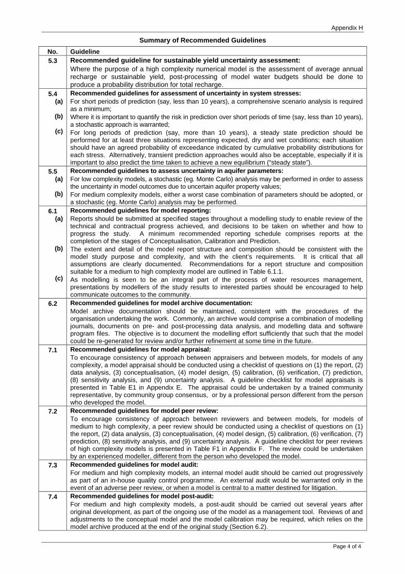
Appendix H

Page 4 of 4


No. Guideline 5.3 Recommended guideline for sustainable yield uncertainty assessment:

Where the purpose of a high complexity numerical model is the assessment of average annual recharge or sustainable yield, post-processing of model water budgets should be done to produce a probability distribution for total recharge.

5.4 (a)

(b)

(c)

Recommended guidelines for assessment of uncertainty in system stresses: For short periods of prediction (say, less than 10 years), a comprehensive scenario analysis is required as a minimum; Where it is important to quantify the risk in prediction over short periods of time (say, less than 10 years), a stochastic approach is warranted; For long periods of prediction (say, more than 10 years), a steady state prediction should be performed for at least three situations representing expected, dry and wet conditions; each situation should have an agreed probability of exceedance indicated by cumulative probability distributions for each stress. Alternatively, transient prediction approaches would also be acceptable, especially if it is important to also predict the time taken to achieve a new equilibrium (“steady state”).

5.5 (a)

(b)

Recommended guidelines to assess uncertainty in aquifer parameters: For low complexity models, a stochastic (eg. Monte Carlo) analysis may be performed in order to assess the uncertainty in model outcomes due to uncertain aquifer property values; For medium complexity models, either a worst case combination of parameters should be adopted, or a stochastic (eg. Monte Carlo) analysis may be performed.

6.1 (a)

(b)

(c)

Recommended guidelines for model reporting: Reports should be submitted at specified stages throughout a modelling study to enable review of the technical and contractual progress achieved, and decisions to be taken on whether and how to progress the study. A minimum recommended reporting schedule comprises reports at the completion of the stages of Conceptualisation, Calibration and Prediction. The extent and detail of the model report structure and composition should be consistent with the model study purpose and complexity, and with the client’s requirements. It is critical that all assumptions are clearly documented. Recommendations for a report structure and composition suitable for a medium to high complexity model are outlined in Table 6.1.1. As modelling is seen to be an integral part of the process of water resources management, presentations by modellers of the study results to interested parties should be encouraged to help communicate outcomes to the community.

6.2 Recommended guidelines for model archive documentation: Model archive documentation should be maintained, consistent with the procedures of the organisation undertaking the work. Commonly, an archive would comprise a combination of modelling journals, documents on pre- and post-processing data analysis, and modelling data and software program files. The objective is to document the modelling effort sufficiently that such that the model could be re-generated for review and/or further refinement at some time in the future.

7.1 Recommended guidelines for model appraisal: To encourage consistency of approach between appraisers and between models, for models of any complexity, a model appraisal should be conducted using a checklist of questions on (1) the report, (2) data analysis, (3) conceptualisation, (4) model design, (5) calibration, (6) verification, (7) prediction, (8) sensitivity analysis, and (9) uncertainty analysis. A guideline checklist for model appraisals is presented in Table E1 in Appendix E. The appraisal could be undertaken by a trained community representative, by community group consensus, or by a professional person different from the person who developed the model.

7.2 Recommended guidelines for model peer review: To encourage consistency of approach between reviewers and between models, for models of medium to high complexity, a peer review should be conducted using a checklist of questions on (1) the report, (2) data analysis, (3) conceptualisation, (4) model design, (5) calibration, (6) verification, (7) prediction, (8) sensitivity analysis, and (9) uncertainty analysis. A guideline checklist for peer reviews of high complexity models is presented in Table F1 in Appendix F. The review could be undertaken by an experienced modeller, different from the person who developed the model.

7.3 Recommended guidelines for model audit: For medium and high complexity models, an internal model audit should be carried out progressively as part of an in-house quality control programme. An external audit would be warranted only in the event of an adverse peer review, or when a model is central to a matter destined for litigation.

7.4 Recommended guidelines for model post-audit: For medium and high complexity models, a post-audit should be carried out several years after original development, as part of the ongoing use of the model as a management tool. Reviews of and adjustments to the conceptual model and the model calibration may be required, which relies on the model archive produced at the end of the original study (Section 6.2).

MURRAY-DARLING BASIN COMMISSION ......This summary introduces groundwater modelling concepts and best practice procedures, outlines how groundwater models can be used to help address

Documents