Multiphase Flow in Pipes Flow Pattern Prediction · Flow Pattern Prediction •Empirical Maps •Ros (1961 –Vertical upward flow) •Govier and Aziz (1972 –Vertical upward flow)

21 – 22 February 2018 Houston, TX

Copyright 2018, Letton Hall Group. This paper was developed for the UPM Forum, 21 – 22 February 2018, Houston, Texas, U.S.A., and is subject to correction by the author(s). The contents of the paper may not necessarily reflect the views of the UPM Forum sponsors or administrator. Reproduction,distribution, or s torage of any part of this paper for commercial purposes without the written consent of the Letton Hall Group is prohibited. Non-commercial reproduction or dis tribution may be permitted, provided conspicuous acknowledgment of the UPM Forum and the author(s) is made. For moreinformation, see www.upmforum.com.

Multiphase Flow in Pipes Flow Pattern Prediction

by Jim Brill

Why is predicting flow patterns so important?

• Required to predict pressure gradient!• Required to size separators/slug catchers• Multiphase Metering and Pumping are sensitive to

flow pattern• Many flow assurance issues depend on flow pattern

• Distribution of paraffin deposition across pipe• Identifying where corrosion might occur• Affects heat transfer/temperature predictions

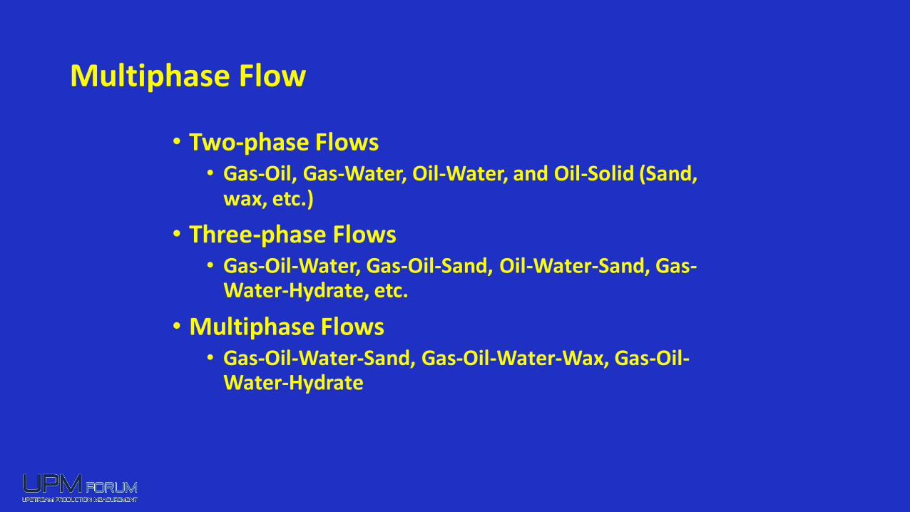
Multiphase Flow

• Two-phase Flows• Gas-Oil, Gas-Water, Oil-Water, and Oil-Solid (Sand,

wax, etc.)

• Three-phase Flows• Gas-Oil-Water, Gas-Oil-Sand, Oil-Water-Sand, Gas-

Water-Hydrate, etc.

• Multiphase Flows• Gas-Oil-Water-Sand, Gas-Oil-Water-Wax, Gas-Oil-

Water-Hydrate

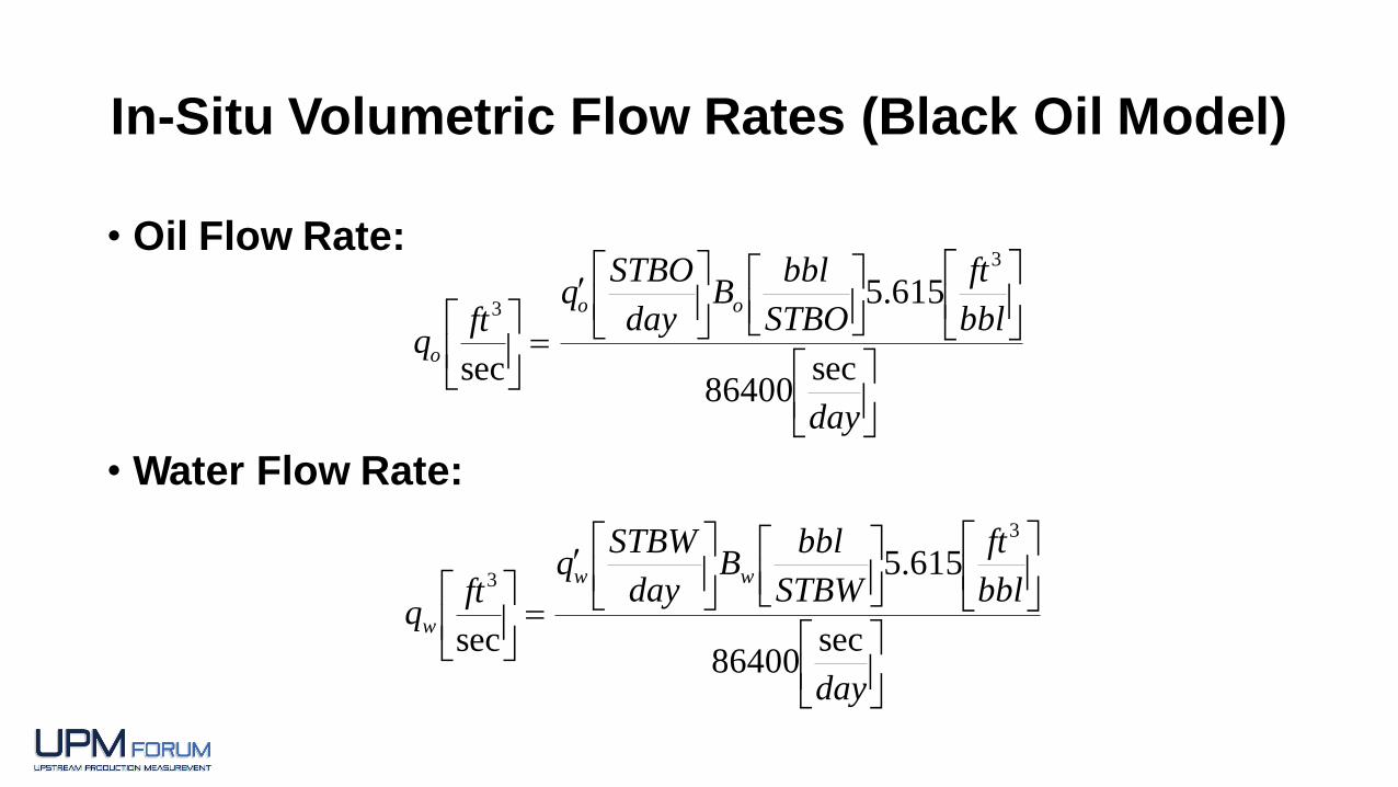
In-Situ Volumetric Flow Rates (Black Oil Model)

• Oil Flow Rate:

• Water Flow Rate:

day

bbl

ft

STBO

bblB

day

STBOq

ftq

oo

osec

86400

615.5

sec

3

3

day

bbl

ft

STBW

bblB

day

STBWq

ftq

ww

wsec

86400

615.5

sec

3

3

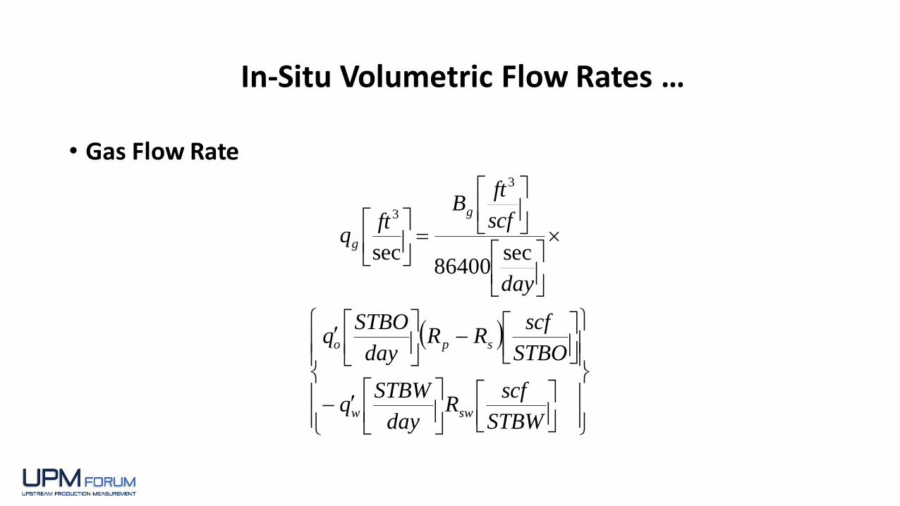
In-Situ Volumetric Flow Rates …

• Gas Flow Rate

STBW

scfR

day

STBWq

STBO

scfRR

day

STBOq

day

scf

ftB

ftq

sww

spo

g

gsec

86400sec

3

3

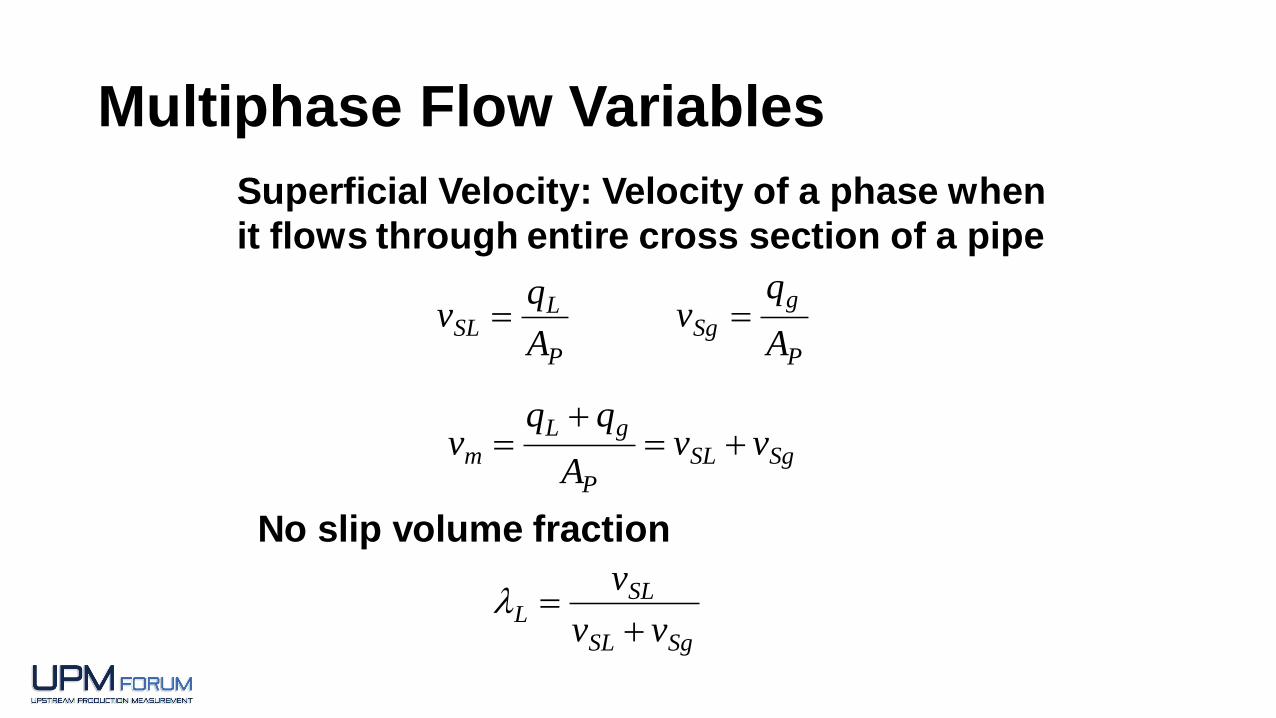
Multiphase Flow Variables

P

LSL

A

qv

P

g

SgA

qv

SgSL

P

gL

m vvA

qqv

SgSL

SLL

vv

v

Superficial Velocity: Velocity of a phase when

it flows through entire cross section of a pipe

No slip volume fraction

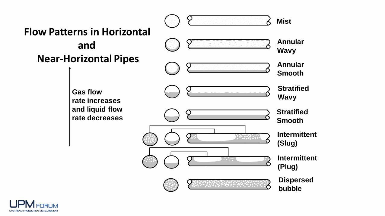
Annular

Smooth

Mist

Stratified

Wavy

Annular

Wavy

Dispersed

bubble

Intermittent

(Plug)

Intermittent

(Slug)

Stratified

Smooth

Gas flow

rate increases

and liquid flow

rate decreases

Flow Patterns in Horizontal and

Near-Horizontal Pipes

Gas flow rate

increases

Dispersed

bubble

Bubble Slug Churn Annular Mist

Flow Patterns in Vertical Pipes

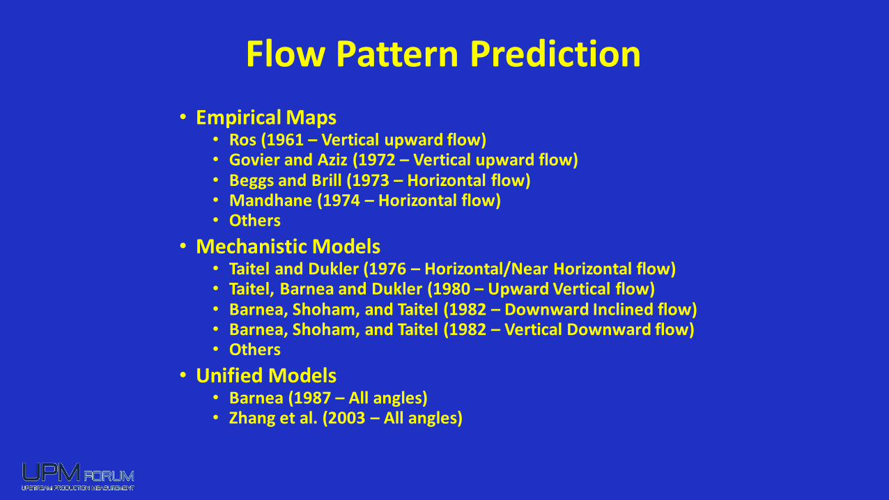
Flow Pattern Prediction

• Empirical Maps • Ros (1961 – Vertical upward flow)• Govier and Aziz (1972 – Vertical upward flow)• Beggs and Brill (1973 – Horizontal flow)• Mandhane (1974 – Horizontal flow)• Others

• Mechanistic Models• Taitel and Dukler (1976 – Horizontal/Near Horizontal flow)• Taitel, Barnea and Dukler (1980 – Upward Vertical flow)• Barnea, Shoham, and Taitel (1982 – Downward Inclined flow)• Barnea, Shoham, and Taitel (1982 – Vertical Downward flow)• Others

• Unified Models• Barnea (1987 – All angles)• Zhang et al. (2003 – All angles)

0.1

1

10

100

1000

0.0001 0.001 0.01 0.1 1

Distributed

Segregated

Intermittent

Transition

L (-)

NF

r,m

2 (-)

L1

L2 L3

L4

Beggs and Brill Empirical Horizontal Flow Pattern Map (1973)

lL =vSL

vmNFR, m =

v2

m

gd

Mandhane Empirical Horizontal Flow Pattern Map (1974)

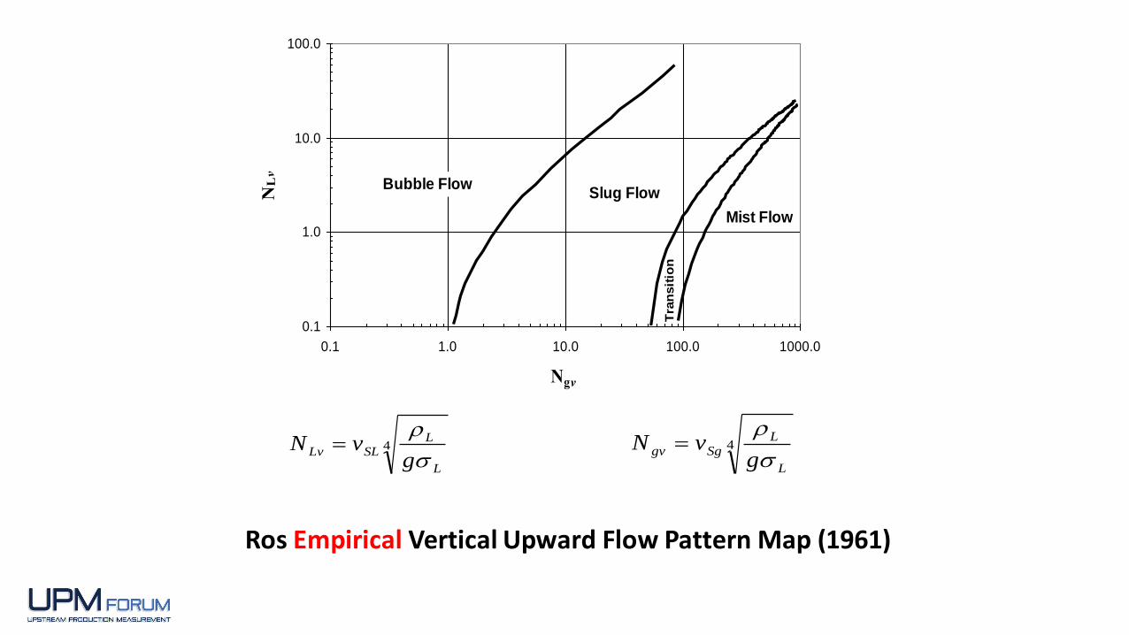
Ros Empirical Vertical Upward Flow Pattern Map (1961)

0.1

1.0

10.0

100.0

0.1 1.0 10.0 100.0 1000.0

Ngv

NLv

Bubble FlowSlug Flow

Mist Flow

Tra

nsit

ion

4

L

LSLLv

gvN

4

L

LSggv

gvN

0.001

0.01

0.1

1

10

0.01 0.1 1 10 100

vSg (m/s)

vS

L (

m/s

)

Dispersed Bubble

BubbleSlug

Annular

Churn

A

B

D E

C

E'

Typical Taitel et al. Mechanistic Vertical Flow Pattern Map (1980)

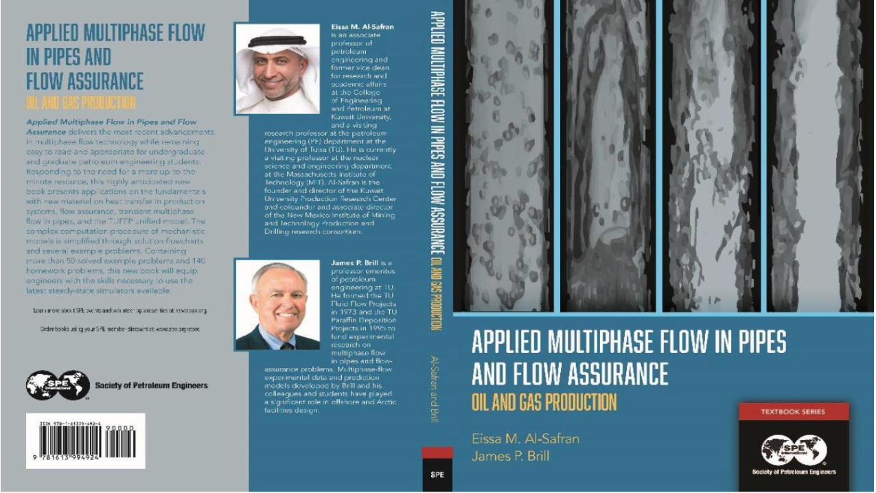
Zhang et al. (2003) Model(Chapter 9 of Applied Multiphase Flow in Pipes and Flow

Assurance – Oil and Gas Production)

• A Unified Model for Prediction of Flow Pattern Transitions and Hydrodynamic Behavior of Gas-Liquid Pipe Flow at all Inclination Angles

• Based on Hydrodynamics of Slug Flow

Slug Flow Pattern Is Surrounded by All Other Flow Patterns

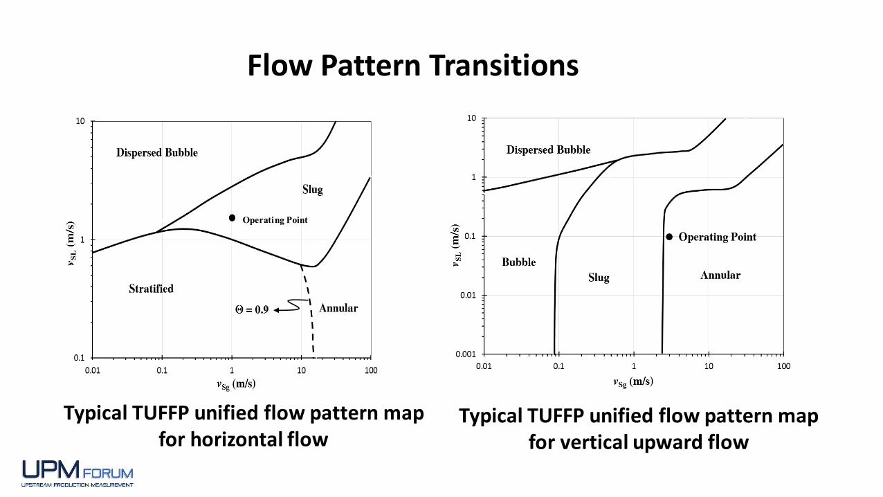
Operating Point

Typical TUFFP unified flow pattern map for horizontal flow

Typical TUFFP unified flow pattern map for vertical upward flow

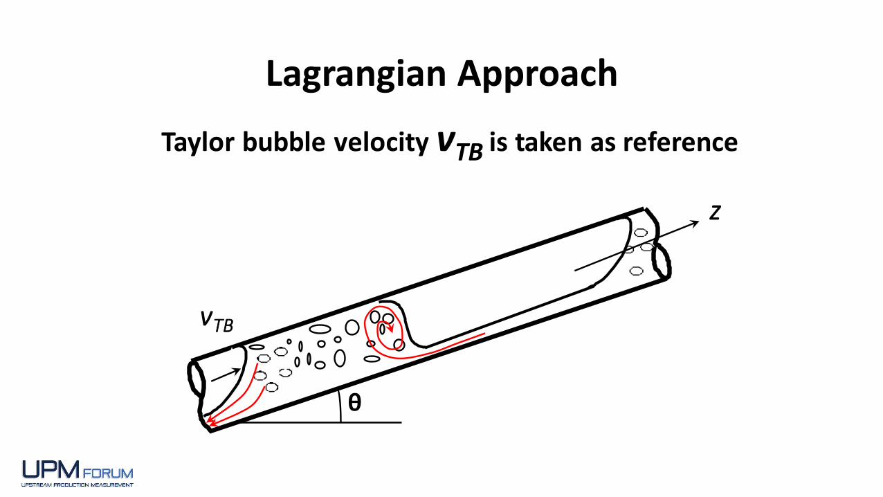
Lagrangian Approach

Taylor bubble velocity vTB is taken as reference

θ

vTB

z

Variables …Af Cross sectional area occupied by liquid film Ac Cross sectional area occupied by gas coreSf Pipe perimeter wetted by liquid film Sc Pipe perimeter contacted by gas core Si Interfacial perimeter

Af

Ac

SfSi

Sc

Liquid film

Gas core

Momentum Equation for Liquid Film

Momentum Equations

Momentum Equation for Gas Core

p2 - p1( )L f

=rc(vTB - vc )(vm - vc )

L f-

t iSi +t cSc(1-HLf )A

- rcgsinq

p2 - p1( )L f

=rL vTB - v f( ) vm - v f( )

L f+

t iSi -t fS f

HLfA- rLgsinq

Momentum Equations ...

Combined Momentum Equation for the liquid film region of a Slug Unit

rL vTB - v f( ) vm - v f( ) - rc vTB - vc( ) vm - vc( )L f

+t cScAc

-t fS f

A f

+t iSi1

A f+

1

Ac

é

ëê

ù

ûú- rL - rc( )gsinq = 0

rc =rg 1- HLf - HLc( ) + rLHLc

1- HLf

where

… Eq. 1

… Eq. 2

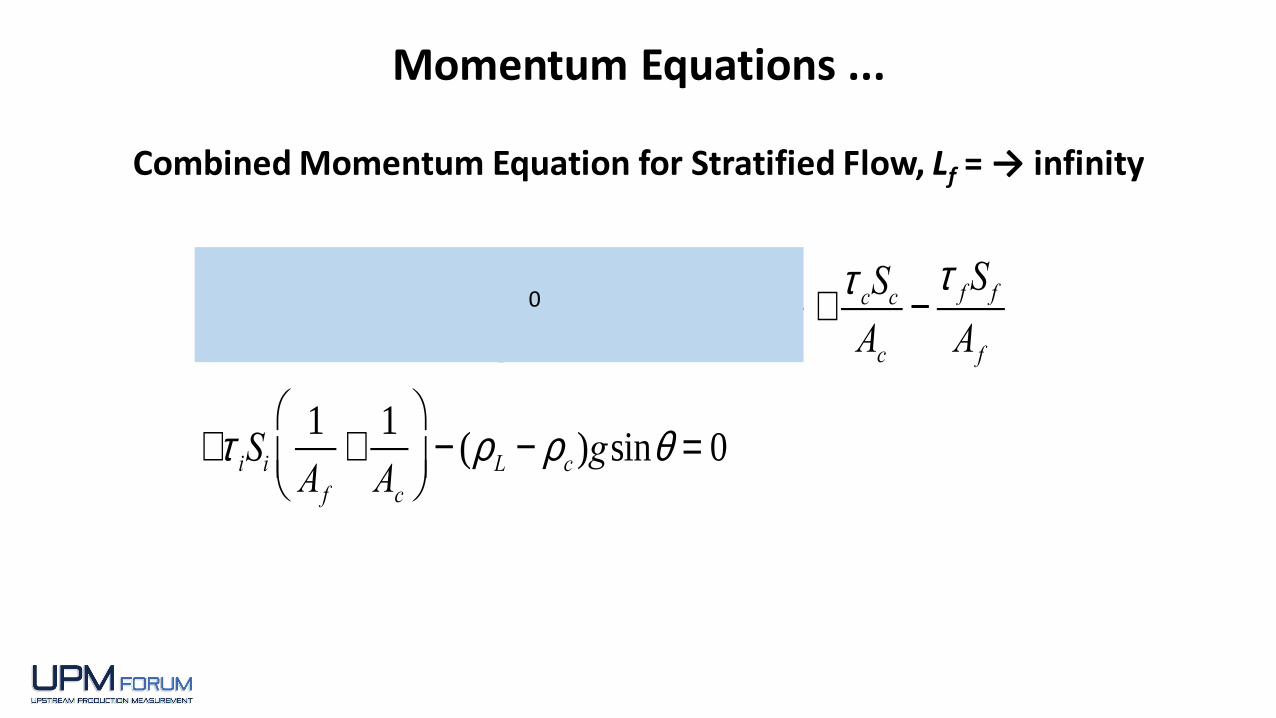
Combined Momentum Equation for Stratified Flow, Lf = → infinity

rL (vTB - v f )(vm - v f )- rc(vTB - vc )(vm - vc )

lF+

t cScAc

-t fS f

A f

+t iSi1

A f+

1

Ac

æ

èç

ö

ø÷ - (rL - rc )gsinq = 0

Momentum Equations ...

0

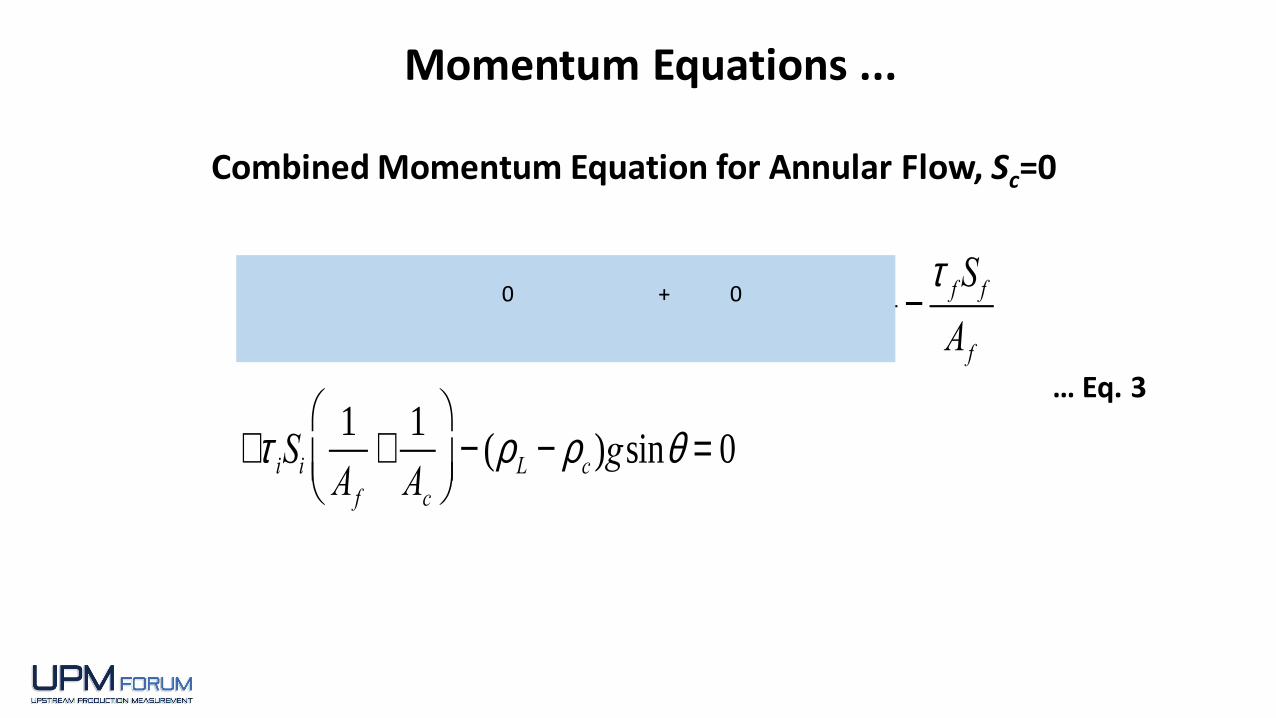
Combined Momentum Equation for Annular Flow, Sc=0

Momentum Equations ...

rL (vTB - v f )(vm - v f ) - rc(vTB - vc )(vm - vc )

lF+

t cScAc

-t fS f

A f

+t iSi1

A f+

1

Ac

æ

èç

ö

ø÷ - (rL - rc )gsinq = 0

0 + 0

… Eq. 3

Flow Pattern Transitions

Operating Point

Typical TUFFP unified flow pattern map for horizontal flow

Typical TUFFP unified flow pattern map for vertical upward flow

Stratified to Annular Flow

Based on concept that as the superficial gas velocity increases, the liquid film climbs up the pipe wall. When the wetted wall Fraction, , reaches 0.9 transition to annular flow is reached.

Thus, a “closure relationship” is required to predict .

Slug to Stratified and/or Annular Flow Boundary(Main difference between Unified and other Mechanistic Models)

Requires trial and error solution of combined momentum equation for the film region of a slug unit or for the combined momentum equation for stratified or annular flow.

Given vSg, find a value of vSL that gives the same value of HLf from these two (or three) equations. This is a difficult calculation, and Torres found an alternative that is new in the unified model.

Torres Alternative

Kinematics – the branch of mechanics treating the motion of bodies in the abstract, and without reference to the action of forces (or momentum balances).

Torres Alternative is based on an equation (HLfk) that is derived from liquid mass balances in the film region and the slug unit.

• Continuity equation for liquid mass flow rate entering and leaving the liquid film region.

• Equations for liquid and gas mass flow rates over a slug unit.• Definition of entrainment fraction to account for liquid entrained in

gas core of film region. • Defines the minimum HLf for slug flow to exist.

Torres Alternative for Slug to Stratified and/or Annular Flow Boundary

HLfk =HLLS vTB - vm( ) + vSLéë ùû vSg + vSL fE( ) - vTBvSL fE

vTBvSg

• Kinematic film holdup = minimum HLf for slugs to exist.• If HLf solution from combined momentum equation for stratified

flow or annular flow > HLfk, then slug flow exists.• At the transition, HLfk = HLf from all combined momentum equations.

… Eq. 4

Empirical Closure Relationships

• Interfacial Friction Factor, fi

• Wetted Wall Fraction, (and interfacial perimeter, Si)

• Liquid Entrainment Fraction, fE

• Slug Liquid Holdup, HLLS

• Slug Translational Velocity, vTB

• Slug frequency (or Slug Length)

Note that these are developed from multiphase flow experiments and may be sensitive to pipe diameter, liquid viscosity, inclination angle, etc.

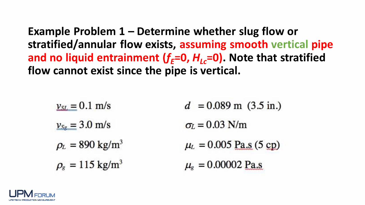
Example Problem 1 – Determine whether slug flow or stratified/annular flow exists, assuming smooth vertical pipe and no liquid entrainment (fE=0, HLc=0). Note that stratified flow cannot exist since the pipe is vertical.

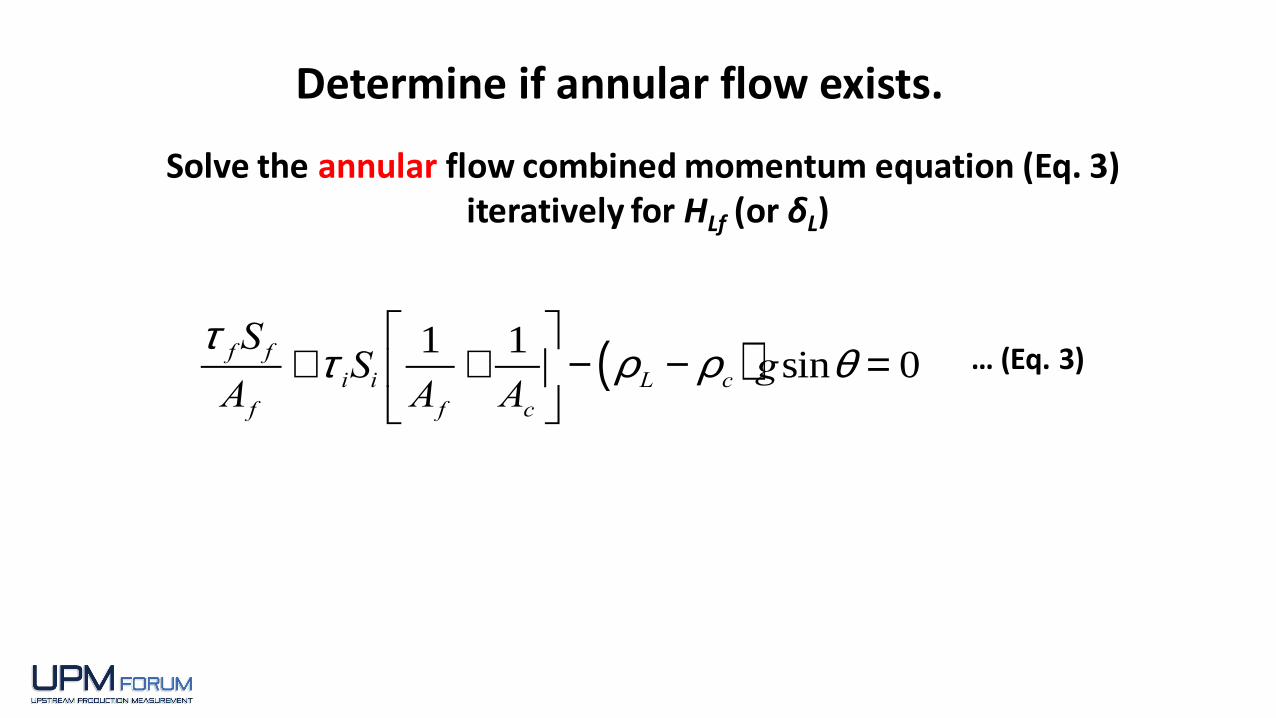
Determine if annular flow exists.

Solve the annular flow combined momentum equation (Eq. 3) iteratively for HLf (or δL)

t fS f

A f+t iSi

1

A f+

1

Ac

é

ëê

ù

ûú- rL - rc( )gsinq = 0 … (Eq. 3)

Variables …Af Cross sectional area occupied by liquid film Ac Cross sectional area occupied by gas coreSf Pipe perimeter wetted by liquid film Sc Pipe perimeter contacted by gas core Si Interfacial perimeter

Af

Ac

SfSi

Sc

Liquid film

Gas core

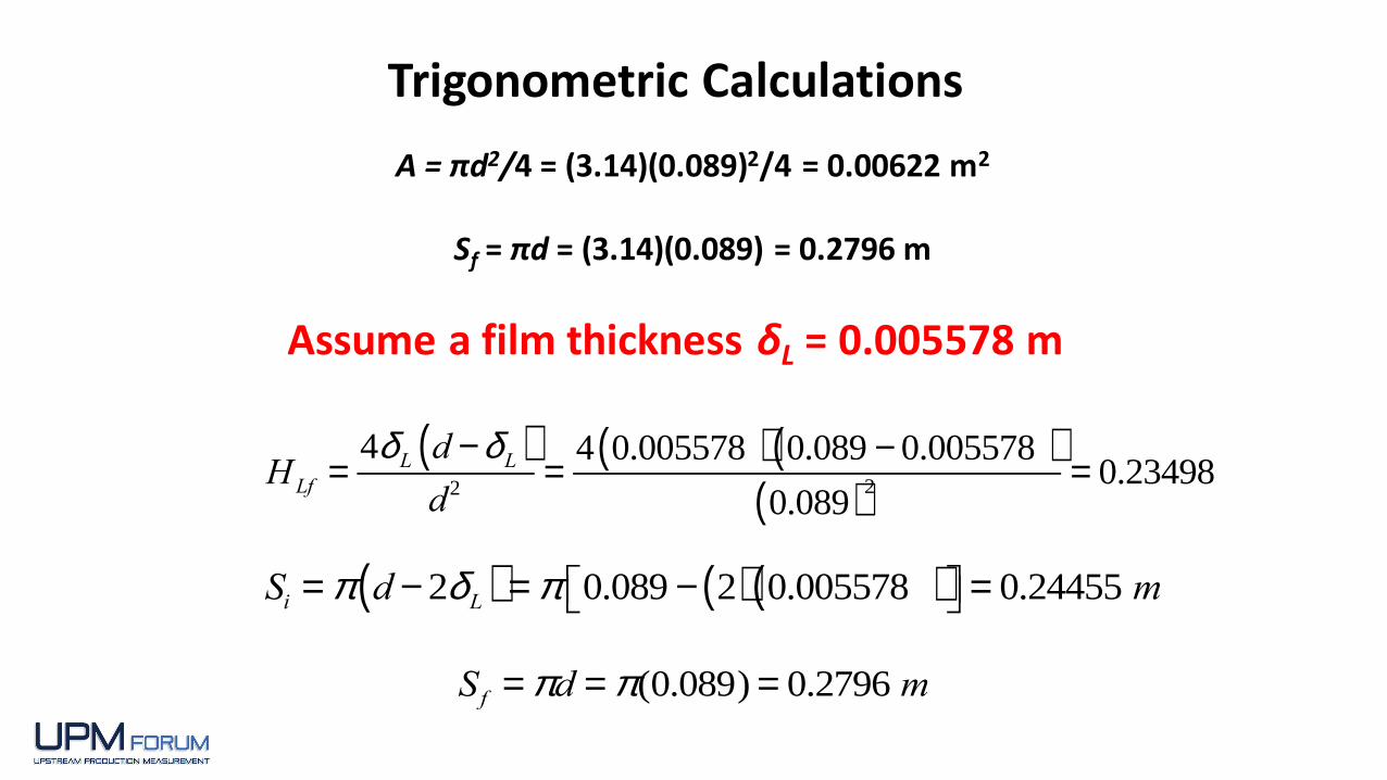
Trigonometric Calculations

A = πd2/4 = (3.14)(0.089)2/4 = 0.00622 m2

Sf = πd = (3.14)(0.089) = 0.2796 m

Assume a film thickness δL = 0.005578 m

HLf =4d L d -d L( )

d2=

4 0.005578 ( ) 0.089 - 0.005578 ( )0.089( )

2= 0.23498

Si = p d - 2d L( ) = p 0.089 - 2( ) 0.005578 ( )éë ùû = 0.24455 m

S f = pd = p(0.089) = 0.2796 m

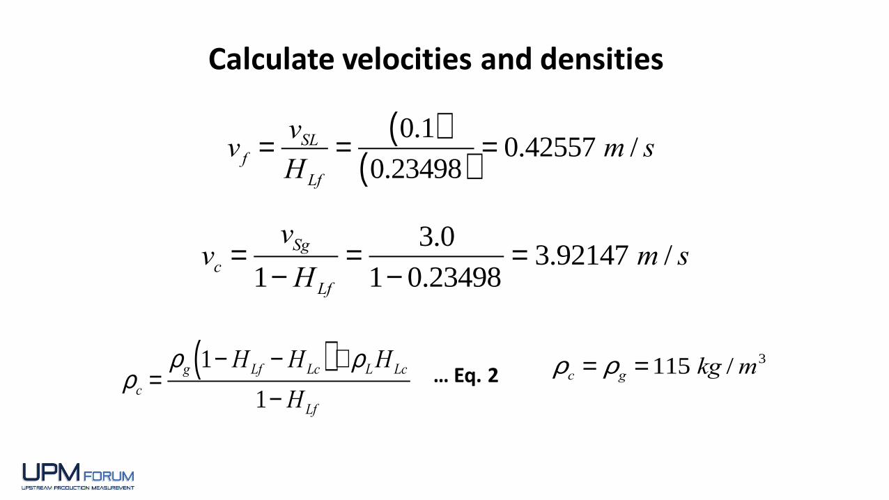
v f =vSL

HLf

=0.1( )

0.23498( )= 0.42557 m / s

Calculate velocities and densities

vc =vSg

1- HLf

=3.0

1- 0.23498= 3.92147 m / s

rc = rg = 115 kg /m3

rc =rg 1- HLf - HLc( ) + rLHLc

1- HLf

… Eq. 2

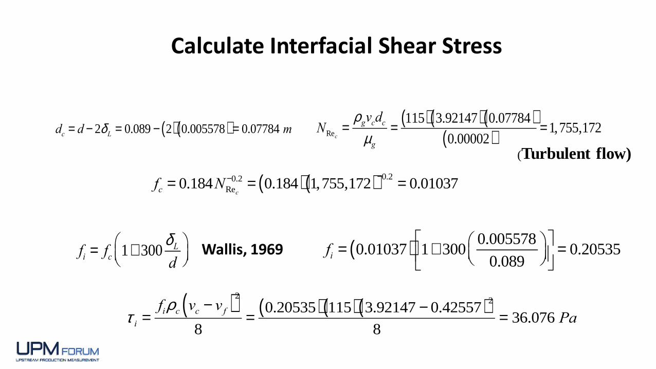
fi = fc 1+ 300d Ld

æ

èçö

ø÷

dc = d - 2d L = 0.089 - 2( ) 0.005578( ) = 0.07784 m NRec=

rgvcdc

mg=

115( ) 3.92147( ) 0.07784( )0.00002( )

= 1,755,172

(Turbulent flow)

fc = 0.184NRec

-0.2 = 0.184( ) 1,755,172( )-0.2

= 0.01037

fi = 0.01037( ) 1+ 3000.005578

0.089

æ

èçö

ø÷é

ëê

ù

ûú = 0.20535Wallis, 1969

t i =firc vc - v f( )

2

8=

0.20535( ) 115( ) 3.92147 - 0.42557( )2

8= 36.076 Pa

Calculate Interfacial Shear Stress

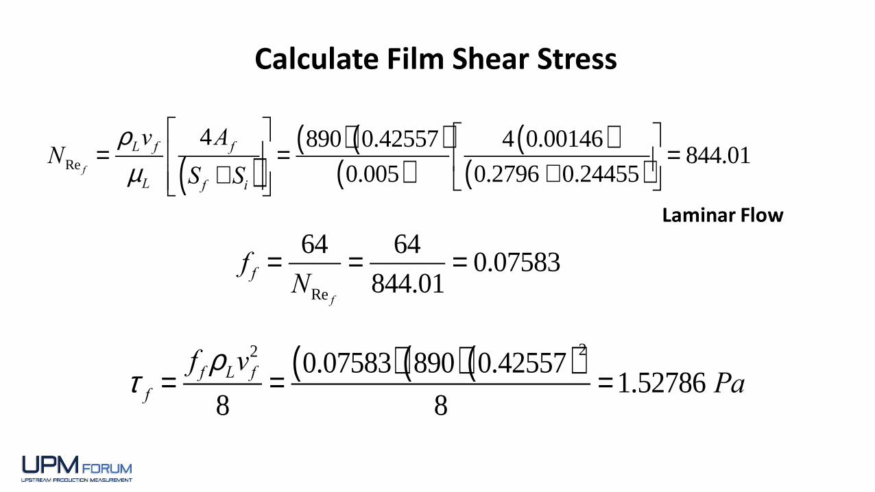
Calculate Film Shear Stress

NRe f=

rLv f

mL

4A f

S f + Si( )

é

ë

êê

ù

û

úú

=890( ) 0.42557( )

0.005( )4 0.00146( )

0.2796 + 0.24455( )

é

ëê

ù

ûú = 844.01

f f =64

NRe f

=64

844.01= 0.07583

t f =f frLv f

2

8=

0.07583( ) 890( ) 0.42557( )2

8= 1.52786 Pa

Laminar Flow

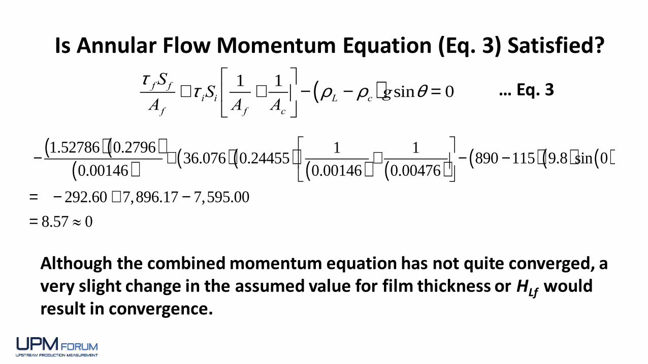
Is Annular Flow Momentum Equation (Eq. 3) Satisfied?

… Eq. 3t fS f

A f+t iSi

1

A f+

1

Ac

é

ëê

ù

ûú- rL - rc( )gsinq = 0

-1.52786( ) 0.2796( )

0.00146( )+ 36.076( ) 0.24455( )

1

0.00146( )+

1

0.00476( )

é

ëê

ù

ûú - 890 -115( ) 9.8( )sin 0( )

= - 292.60 + 7,896.17 - 7,595.00

= 8.57 » 0

Although the combined momentum equation has not quite converged, a very slight change in the assumed value for film thickness or HLf would result in convergence.

vTB = covm + 0.54 gd cosq + 0.35 gd sinqNicklin (1962) and Bendickson (1984)

vTB = 1.2vm + 0.35 gd sin 90( )éë

ùû = 1.2( ) 3.1( )+ 0.35 9.8( ) 0.089( ) = 4.047 m / s

Determine HLfk from Eq. 4 with fE = 0.0

HLfk =HLLS vTB - vm( ) + vSLéë ùû

vTB=

0.807( ) 4.047 - 3.1( ) + 0.1éë ùû

4.047= 0.2135

Since HLf from the annular flow combined momentum balance equation (0.23498), is greater than HLfk (0.2135) for slug flow to occur, the flow pattern is slug.

Calculate Kinematic Film Liquid Holdup, HLfk

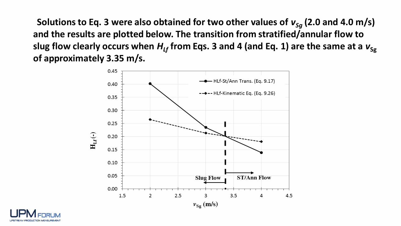
Solutions to Eq. 3 were also obtained for two other values of vSg (2.0 and 4.0 m/s) and the results are plotted below. The transition from stratified/annular flow to slug flow clearly occurs when HLf from Eqs. 3 and 4 (and Eq. 1) are the same at a vSg

of approximately 3.35 m/s.

Note that this is Example 9.3 of the new SPE Textbook. See the Textbook for calculation of the

Pressure Gradient for slug flow.

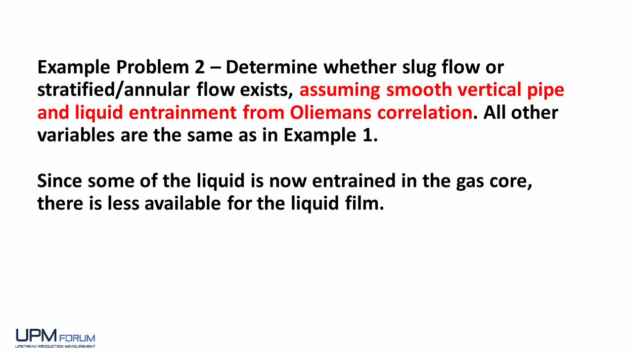
Example Problem 2 – Determine whether slug flow or stratified/annular flow exists, assuming smooth vertical pipe and liquid entrainment from Oliemans correlation. All other variables are the same as in Example 1.

Since some of the liquid is now entrained in the gas core, there is less available for the liquid film.

Torres Alternative for Slug to Stratified and/or Annular Flow Boundary

HLfk =HLLS vTB - vm( ) + vSLéë ùû vSg + vSL fE( ) - vTBvSL fE

vTBvSg

• Kinematic film holdup = minimum HLf for slugs to exist.• If HLf solution from combined momentum equation for stratified

flow or annular flow > HLfk, then slug flow exists.• At the transition, HLfk = HLf from all combined momentum equations.

… Eq. 4

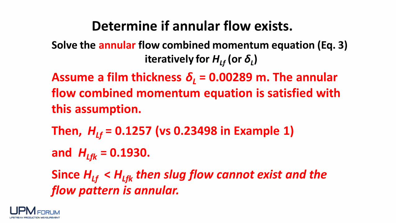
Determine if annular flow exists.Solve the annular flow combined momentum equation (Eq. 3)

iteratively for HLf (or δL)

Assume a film thickness δL = 0.00289 m. The annular flow combined momentum equation is satisfied with this assumption.

Then, HLf = 0.1257 (vs 0.23498 in Example 1)

and HLfk = 0.1930.

Since HLf < HLfk then slug flow cannot exist and the flow pattern is annular.

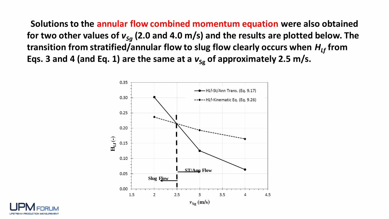
Solutions to the annular flow combined momentum equation were also obtained for two other values of vSg (2.0 and 4.0 m/s) and the results are plotted below. The transition from stratified/annular flow to slug flow clearly occurs when HLf from Eqs. 3 and 4 (and Eq. 1) are the same at a vSg of approximately 2.5 m/s.

ST/Ann Flow

Slug Flow

Clearly, closure relationships can have a significant impact on predicting flow pattern and pressure gradient. For this reason, much of the TUFFP research program is now devoted to developing improved closure relationships for various pipe diameters, inclination angles, oil viscosities, wetting angle at pipe wall in stratified flow, etc.

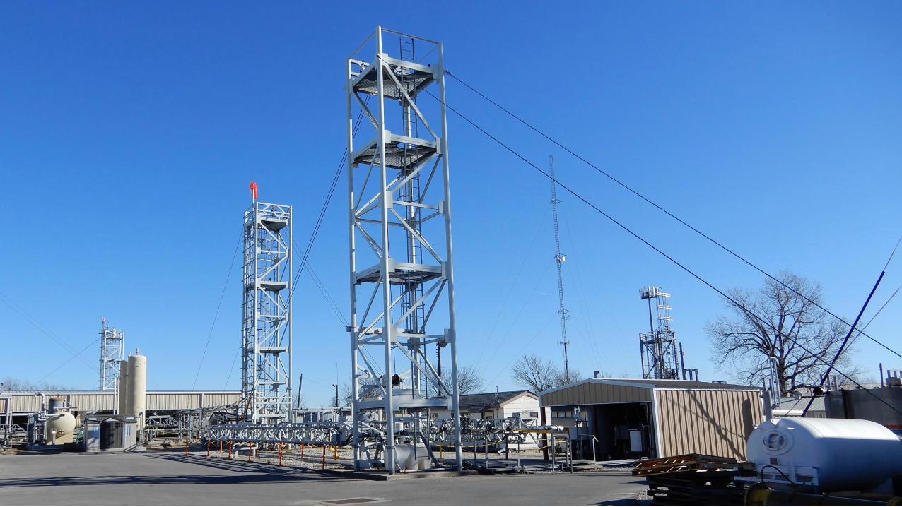
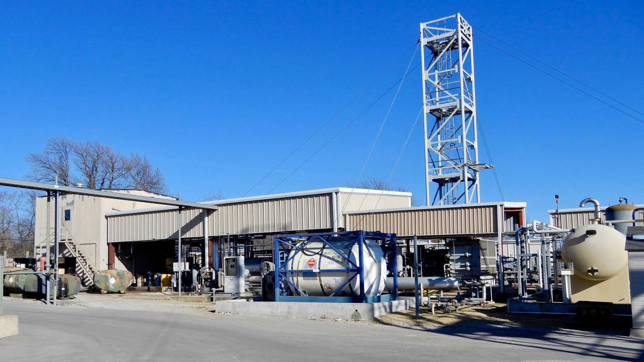
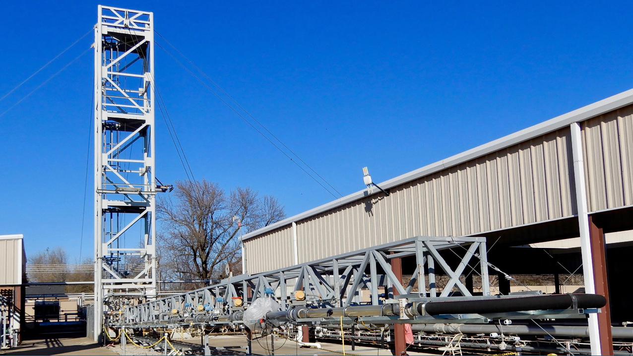
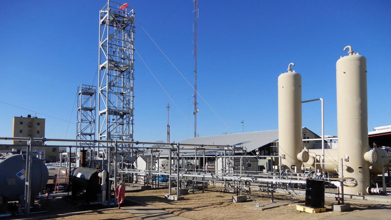
TUFFP Experimental Facilities

For

Developing Improved

Closure Relationships

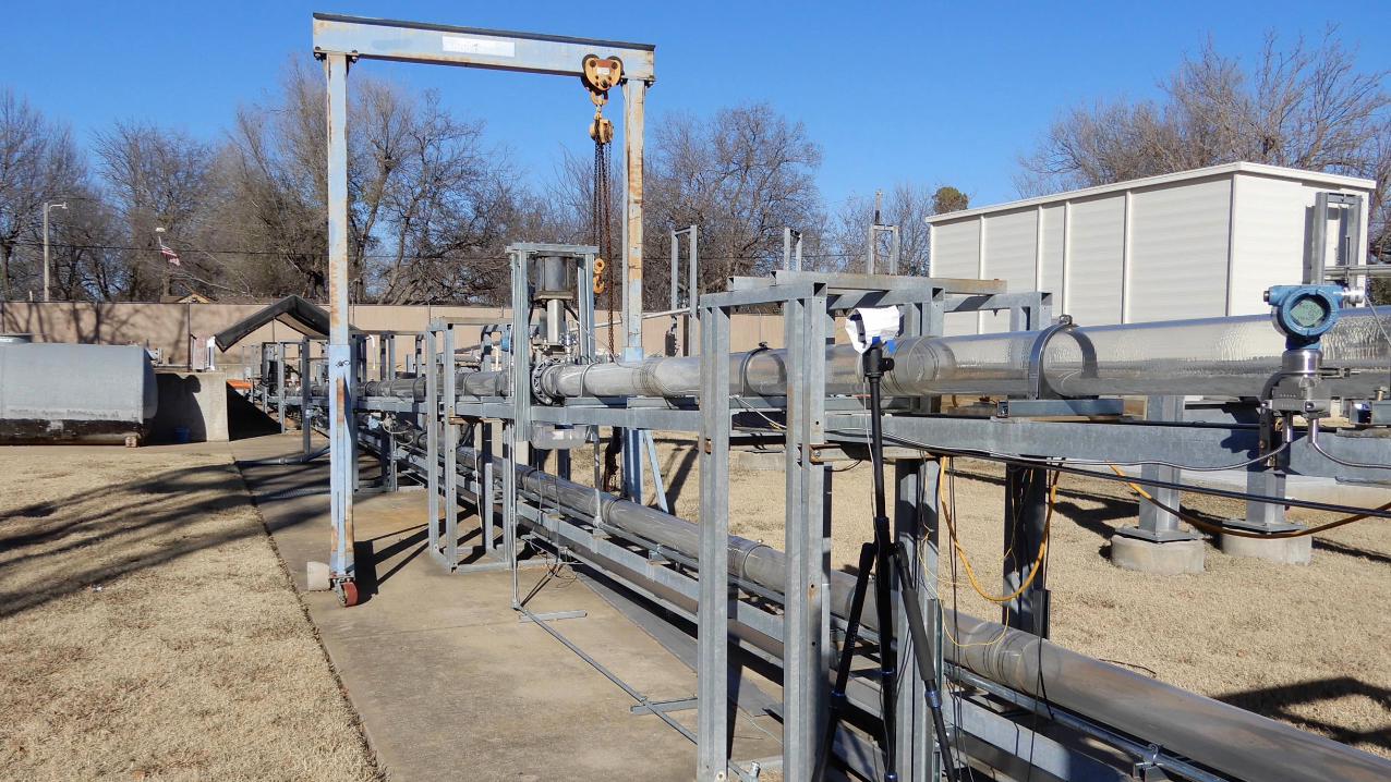
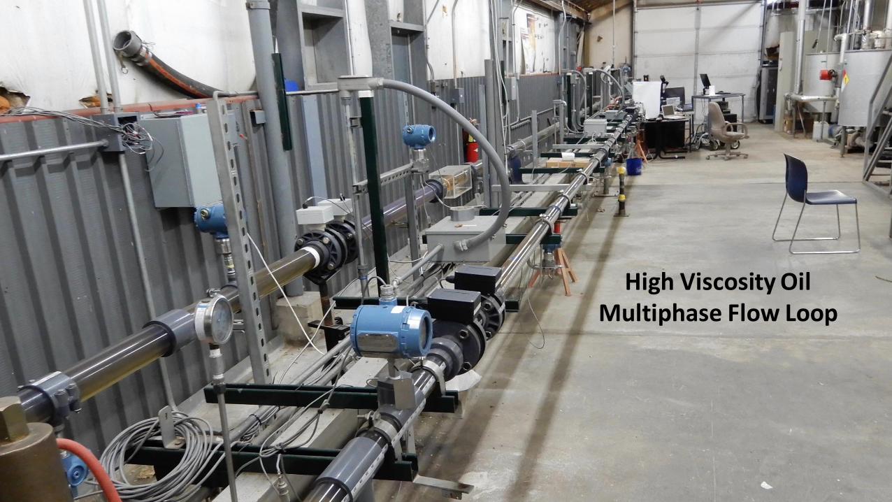
High Viscosity OilMultiphase Flow Loop

Paraffin DepositionSingle-Phase Liquid

Flow Loop

Horizontal Well Artificial Lift Flow Loop

Hydrate Flow Loops