Multimedia Information Retrieval. p. 2 Problem On the Web and in local DBs a large amount of information is not textual: audio (speech, music…) images,

Multimedia Information Retrieval

p. 2

Problem

On the Web and in local DBs a large amount of information is not textual:

audio (speech, music…) images, video, …

How can we efficiently retrieve multimedia information?

p. 3

Application examples

Web indexing: Multimedia retrieval from the Web Identify and ban (illegal or unauthorized) ads and

images Trademark & copyright Interactive museums Commercial DBs

p. 4

Application examples[2]

Satellite images (military, government, …) Medical images Entertainment Criminal investigation (scene analysis, face

recognition, ..) …

p. 5

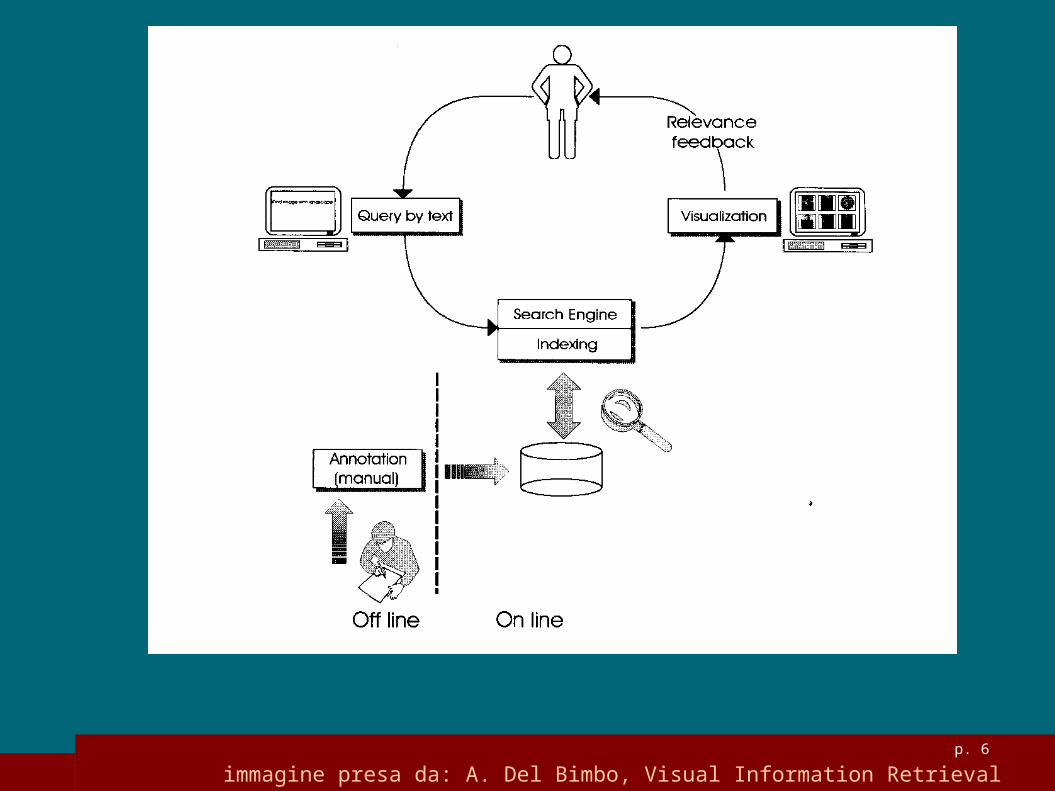
First generation multimedia information retrieval systems

Off-line: multimedia documents are associated with a textual description Ex.: Manual annotation (“content descriptive

metadata”) The text surrounding an image in the document

(e.g. figure caption) On-line: using textual IR based on “keyword

match” (Google image)

p. 6

immagine presa da: A. Del Bimbo, Visual Information Retrieval

p. 7

Limitation of textual approach

Manual annotation on large multimedia DBs is unfeasible

Describing a scene or an audio is highly subjective (different annotators might perceive/highlight different details)

p. 8

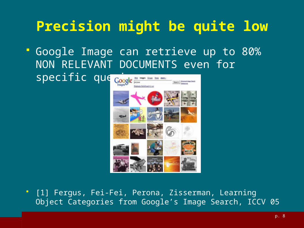
Precision might be quite low

Google Image can retrieve up to 80% NON RELEVANT DOCUMENTS even for specific queries

[1] Fergus, Fei-Fei, Perona, Zisserman, Learning Object Categories from Google’s Image Search, ICCV 05

p. 9

…&Recall

Many relevant images (videos, audio) are not retrieved

p. 10

Current state-of-the-art retrieval models…

“Content Based” systems: Ignore the textual phase User query might be non-textual Model perceptual similarity bewteen the

query and the multimedia document Still limited to DBs (does not scale on the

Web)

p. 11

Examples of multimedia search queries

Find a song by singing the refrain Retrieving some soccer action frame

in a sport video Searching a paint with some

specific detail or texture or painting technique (e.g chiaroscuro)

…

p. 12

Current state-of-the-art retrieval models…[2]

Automated image annotation: Pre-processing (“information

extraction”): automatically extract some information from the image and associate it to some textual label

Retrieval is then a “traditional” text retrieval

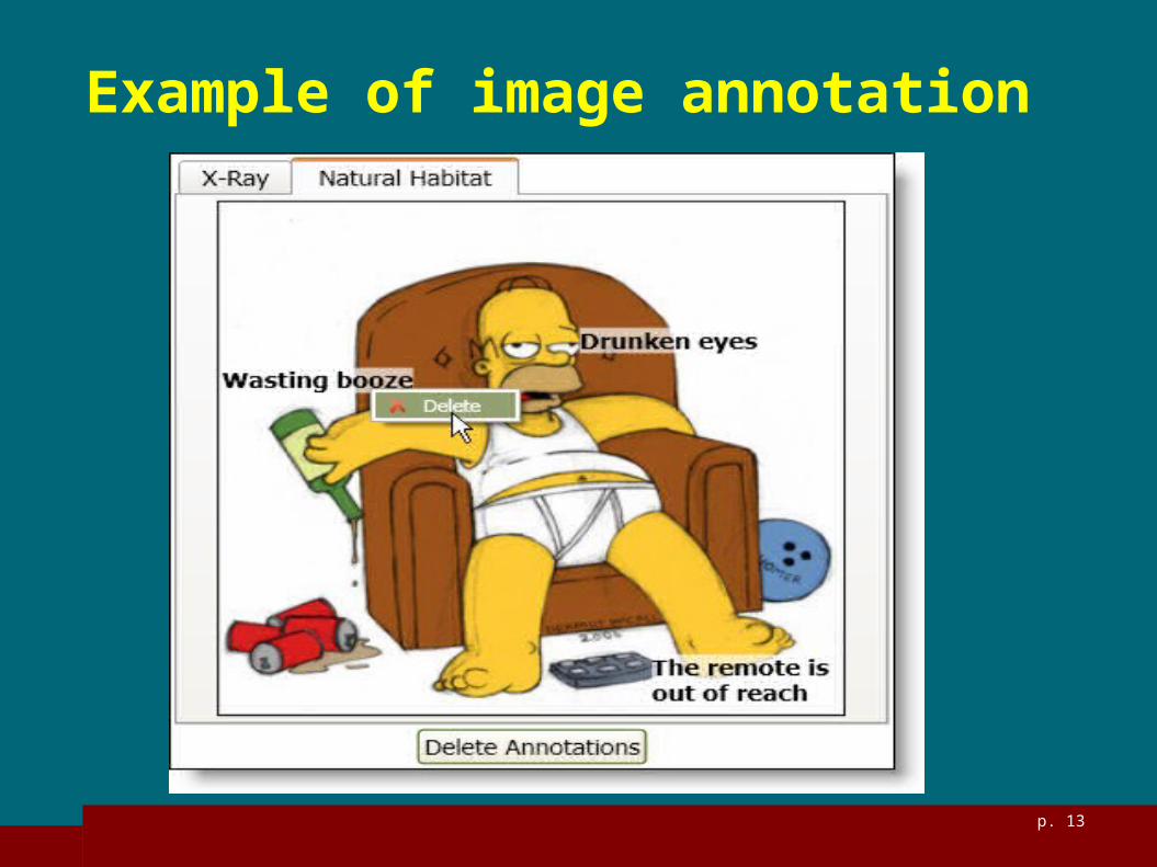
p. 13

Example of image annotation

p. 14

Image Retrieval wrt textual Retrieval

Analysis and representation of non-symbolic information

A text can be seen as a combination of atomic symbolic elements (words or tokens)

An image is a collection of non-symbolic elements (pixels) and an audio is represented as a wave ..there is no vocabulary of basic meaning elements, as for text!

p. 15

Basic elements of a Content Based Multimedia IR

On the users side: The query is a multimedial object (an image a

sketch an audio frame..) The output is an ordered list of element ranked

according to perceptual similarity wrt the query There are a variety of optional interactive features

to visualize image collections or give a feedback to the system

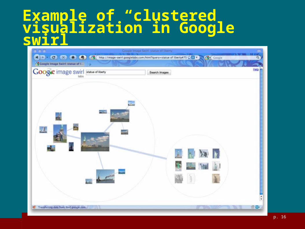
p. 16

Example of “clustered” visualization in Google swirl

p. 17

Query by image example

The query is anImage detail

p. 18

Query by image example [2]

Note that the queryand the detail mightnot perfectly match,e.g. the query can be chosen from andimage prior toa restoration of the picture

p. 19

Query by sketch

immagine presa da: A. Del Bimbo, Visual Information Retrieval

p. 20

Basic elements of a Content Based Multimedia IR [2]

From the “system” perspective: Representation of the multimedia object (e.g.

what is the feature space) Modeling the notion of perceptual similarity

(e.g., trough specific matching algorithms) Efficient indexing of feature space (the

“vocabulary” is order of magnitude higher than for words)

Relevance feedback and visualization interface

p. 21

MULTIMEDIA OBJECT REPRESENTATION

p. 22

Representing an image through a set of features

As for text, a feature is a representation, through a vector of elements, of the image (or a detail l’ )

If I' is an image detail, then a feature f for l’ is defined as:f(I') Rk, f(I') = (v0, … vk-1)T,

k >= 1

p. 23

Representing an image through a set of features [2]

In general, a feature is a measurable characteristic of an image

The image is then represented using the measurable values of its selected features f1, …, fn

p. 24

Local and global features

I' = I: global feature (remember I image I’ detail)

I' I: local feature

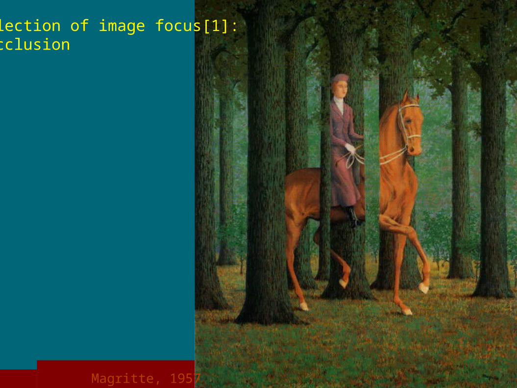
Local Features : How to select relevant image parts that we want

to represent (I‘1, I‘2, …) Loca features allows it to cope with missing

elements, occlusions , background..

p. 25

Main problems in image representation Selecting features is crucial Just as for text, the same meaning can be

conveyed by apparently very different images (different according to specific features)

But the problem of “variability” is much harder

p. 26

variability[1]: orientation and rotation

Michelangelo 1475-1564

p. 27

Variability [2]: lightening and brightness

p. 28

Variability [3]: deformation

Xu, Beihong 1943

p. 29

Variability [4]: intra-class variability

p. 30

Selection of image focus[1]: occlusion

Magritte, 1957

p. 31

Klimt, 1913

Selection of image focus[2]: background separation

p. 32

Example: local feature

fi(I') I'

I

immagine presa da: Tutorial CVPR 07

p. 33

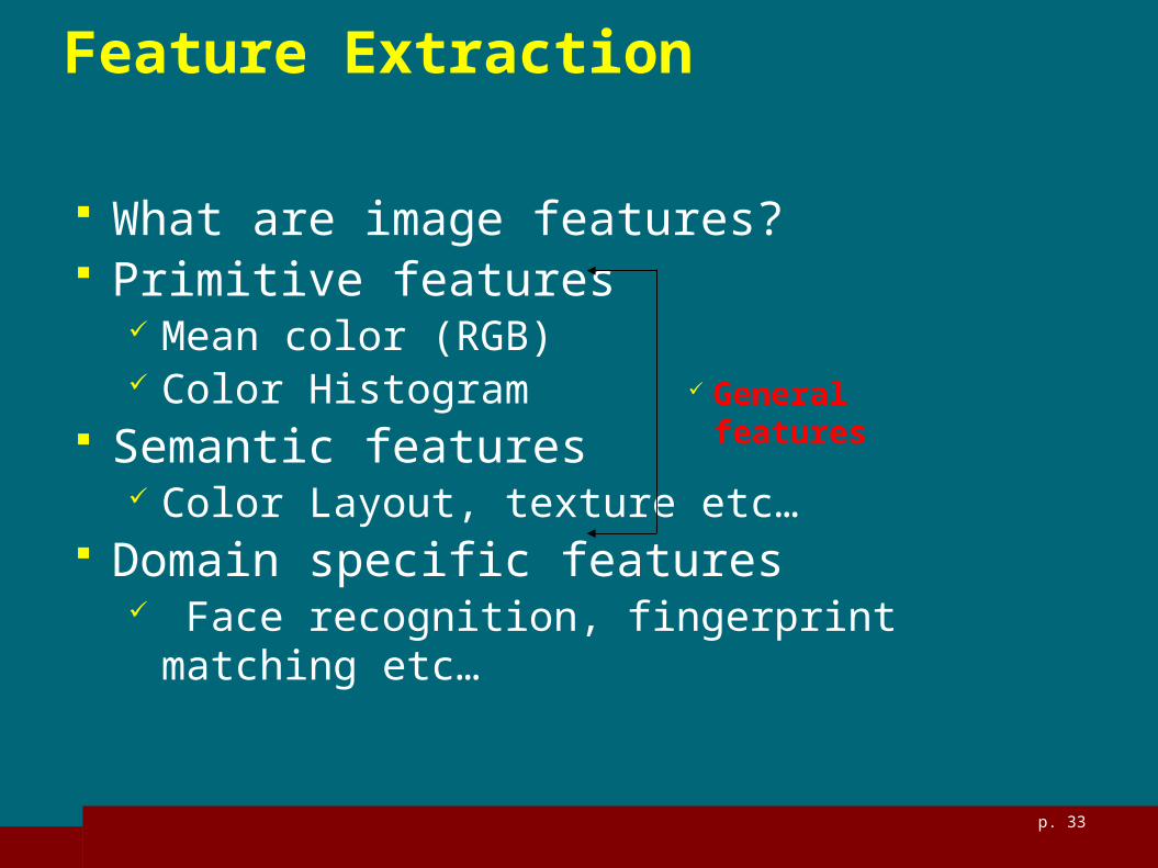
Feature Extraction

What are image features? Primitive features

Mean color (RGB) Color Histogram

Semantic features Color Layout, texture etc…

Domain specific features Face recognition, fingerprint matching etc…

General features

p. 34

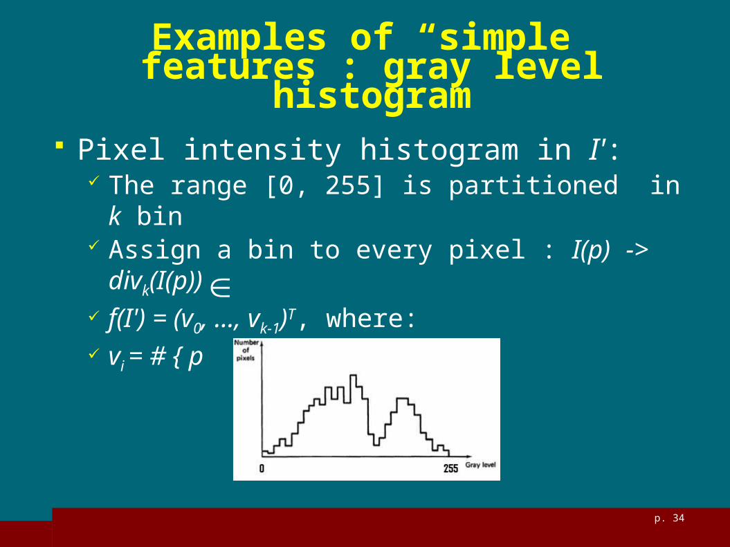
Examples of “simple” features : gray level histogram

Pixel intensity histogram in I': The range [0, 255] is partitioned in k bin Assign a bin to every pixel : I(p) -> divk(I(p)) f(I') = (v0, …, vk-1)T, where: vi = # { p I’ : divk(I(p)) = i}

p. 35

Frequency count of each individual color Most commonly used color feature

representation

Image

Corresponding histogram

Example

p. 36

Examples of “domain-specific” features : facial metrics

f(I) = (d1 , d2 , d3 , d4)T

p. 37

More features

shape texture

p. 38

Feature space

If we now use n features in R, then I can be represented as a feature vector x(I) = (f1(I), …fn(I))T

x(I) is a point in Rn, the feature space

p. 39

Feature Space [2]

More in general, if :fi(I) Rk, (a single feature is a k multidimensional

vector ) Then : x(I) = (f1(I) T … fn(I) T)T is a point in

Rn*k

p. 40

Ex.: Feature space(R2)

p. 41

Feature Space[3]

The concept of feature space is similar BUT NOT IDENTICAL TO vector space model as in traditional IR (where real values are the tf*idf of words in document collection)

It is the most common, but not the unique, representation in content-based multimedia IR

p. 42

SIMILARITY

p. 43

Perceptual similarity

In text retrieval, similarity between two documents is modeled as a function of the common words in the two documents (e.g. cosine similarity with tf*idf feature vectors)

In multimedia retrieval a similar notion of “distance” between vectors is applied…

p. 44

Perceptual similarity [2]

In the feature space, similarity is (inversely) proportional to a distance measure between feature vectors (not necessarily an Euclidean distance): dist(x(I1),x(I2))

Given the query Q, the system output is an image list I1, I2, … ordered according to:I1 = arg minI dist(x(Q),x(I)), …

p. 45

Example(R2)

p. 46

Perceptual similarity [3]

Other matching algorithms use more complex representations or more complex similarity functions, which are usually dependent on the type of multimedia object and retrieval tasks

p. 47

INDEXING

p. 48

Indexing

Problem: efficiently index the data of a multi-dimensional space?

Several data structures (as IR keyword dictionary) are indexed using some ordering (e.g. alphabetic ordering): xi <= xj V xj <= xi (0 <= i,j <= N)

In Rk this cannot be done (remember every feature is multi-dimensional!)

p. 49

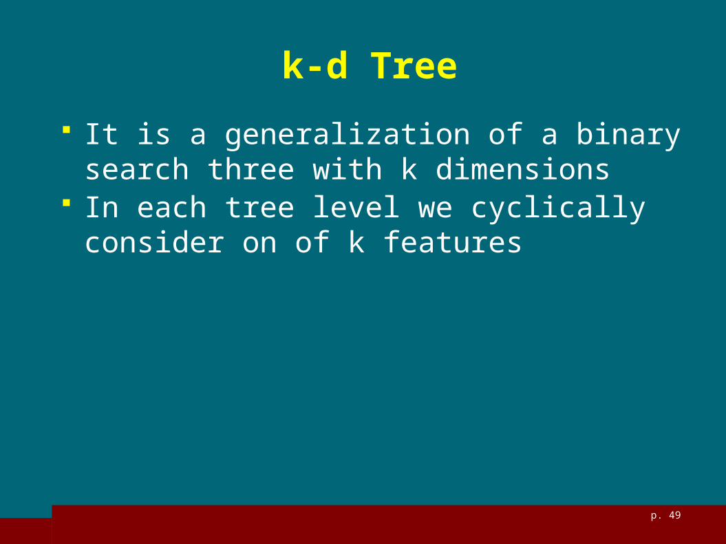
k-d Tree

It is a generalization of a binary search three with k dimensions

In each tree level we cyclically consider on of k features

p. 50

k-d Tree [2]

Suppose we wish to index a set of N k-dimensional points:

P1, …, PN, Pi Rk, Pi =(xi1, …, xi

k)

We select the first dimension (feature) and find the value L1, which is the median of x1

1, …, xN

1

p. 51

k-d Tree [3] The root of the tree includes L1 The left sub-tree (TL) includes the points Pi

s.t. xi1 <= L1

The left sub-tree (TR) wiIl include all the other points

At level 1, we select the second feature and, separately for TL e TR, we compute L2 and L3, selected such that : L2 i is median wrt the elements i xj1

2, xj22, …

of TL

L3 is the median of the elements in TR

p. 52

k-d Tree [4]

When the last k feature (point) has been considered, we backtract and cyclically consider agaion the first feature

Points are associated to the tree leaves

p. 53

Example

immagine presa da: Hemant M. Kakde, Range Searching using Kd Tree

We start with a set of 2-dimensional points. In L1, P5 ‘s x coordinate is the median of the dataset In L2, P2 is the median of y values in the partition, and in L3 P7 We then consider again x values, and in L4 the median is again P2 etc.

p. 54

IMAGE, VIDEO E AUDIO RETRIEVAL

p. 55

..So far

We analyzed: Query types Feature types Similarity functions Indexing methods

Now we present retrieval methods Retrieval strategies clearly depend upon the

multimedia object representation technique

p. 56

Retrieval by color: color histograms

We can represent an image through the color histogram of an image part I‘ (we already seen how histograms are created for grey images): A single pixel can be represented with different

encodings P: RGB, HSV, CIE LAB, … Every channel (values range) is partitioned in k

bin: f(I') = (r0,…, rk-1, g0, …, gk-1, b0, …, bk-1)T, ri = # { p in I’: divk(R(p)) = i }, gi = # { p in I’: divk(G(p)) = i }, bi = # { p in I’: divk(B(p)) = i }

p. 57

Color histograms [2]

Alternatively , we divide RGB in k3 bin:

f(I') = (z0,…, zh-1)T, h= k3 the # of combinations of 3 values

If zi represents the triple of RGB values (i1, i2, i3), then :

zi = # { p in I’: divk(R(p)) = i1 and divk(G(p)) = i2and divk(B(p)) = i3 }

p. 58

Color histogram [3]: example (4 bins)

immagine presa da: Wikipedia

p. 59

Retrieval by texture

p. 60

Statistical Approach

Tamura features: based on the analysis of the local intensity distribution of the image, in order to measure perceptual characteristics of the feature, such as a

Contrast Granularity Direction

p. 62

Video retrieval

A video is a sequence of images Every image is called FRAME

p. 63

Elements of a video

Frame: a single image Shot: A sequence of frames taken from a

single camera Scene: a set of consecutive shots that

reflect the same space, time and action

p. 64

Videosequence segmentation

If we can automatically identify “editing effects” (cuts, dissolvenze, ….) among shots, we can the automatically partition a video in shots

Identifying scenes is much more complicated, since this is a “semantic” concept

p. 65

Video search

Videos can be represented efficiently using “key frame” which are representative of every shot

A key frame can then be treated and processed as a “still image”: We can then apply all what we have just seen for

single images

p. 66

Video search

Alternatively, we can search in a video a specific “motion” (e.g., a specific trajectory of a soccer action, …)

p. 67

Audio retrieval

Several types of audio: Spoken audio

A whatever audio signal within the frequence range that can be perceived by the human ears (e.g. a thunderstorm)

Music: We must model the different instruments , musical effects,

etc.

p. 68

Audio Query types

Query by example: the input is an audio file, used to search “similar” files

Query by humming: User sings the searched melody

p. 69

Represenattion and similarity

The feature space can be obtained using e.g. histograms obtained from the spectral representation of the signal

Perceptual similarity is computed as the distance among multidimensional points, as for images Distance metrics: Euclidean, Mahalanobis,

histogram distance measures (Histogram Intersection, Kullback-Leibler divergence, ki-square, etc.)

p. 70

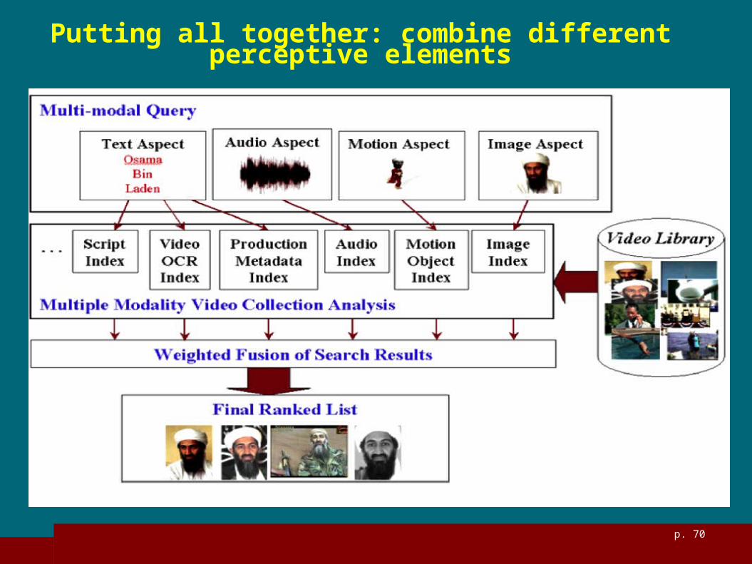
Putting all together: combine different perceptive elements

p. 71

Content Based systems: limitations

All the information concerning the target multimidia objects is provided by the query (e.g., a given shape, or color, or audio signal)

p. 72

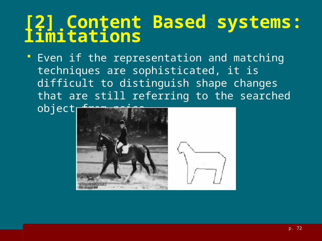
[2] Content Based systems: limitations Even if the representation and matching techniques are

sophisticated, it is difficult to distinguish shape changes that are still referring to the searched object from noise

p. 73

Limitations of Content Based systems [3] Human brain can distinguish among different shapes of

the same object only after having seen several objects of the same type in different positions

To obtain similar perfromances, artificial systems need to be trained to recognize objects using machine learning algorithms for:

Automated image annotation Automated image classification

p. 74

references

A. Del Bimbo, Visual Information Retrieval, Morgan Kaufmann Publishers, Inc. San Francisco, California", 1999

Forsyth, Ponce, Computer Vision, a Modern Approach 2003

p. 75

references[2]

Smeulders et al., Content-Based Image Retrieval at the End of Early Years, IEEE PAMI 2000

Long et al., Fundamentals of Content-based Image Retrieval, in: D. D. Feng, W. C. Siu, H. J. Zhang (Ed.),Multimedia Information Retrieval & Management-Technological Fundamentals and Applications, Springer-Verlag, New York(2003)

Foote et al., An Overview of Audio Information Retrieval, ACM Multimedia Systems, 1998

Hemant M. Kakde, Range Searching using Kd Tree, 2005