Physica A 316 (2002) 87 – 114 www.elsevier.com/locate/physa Multifractal detrended $uctuation analysis of nonstationary time series Jan W. Kantelhardt a; b ; * , Stephan A. Zschiegner a , Eva Koscielny-Bunde c; a , Shlomo Havlin d; a , Armin Bunde a , H. Eugene Stanley b a Institut f ur Theoretische Physik III, Justus-Liebig-Universit at Giessen, Heinrich-Bu-Ring 16, D-35392 Giessen, Germany b Department of Physics, Center for Polymer Studies, Boston University, Boston, MA 02215, USA c Potsdam Institute for Climate Impact Research, P.O. Box 60 12 03, D-14412 Potsdam, Germany d Department of Physics and Gonda-Goldschmied-Center for Medical Diagnosis, Bar-Ilan University, Ramat-Gan 52900, Israel Abstract We develop a method for the multifractal characterization of nonstationary time series, which is based on a generalization of the detrended $uctuation analysis (DFA). We relate our multifractal DFA method to the standard partition function-based multifractal formalism, and prove that both approaches are equivalent for stationary signals with compact support. By analyzing several examples we show that the new method can reliably determine the multifractal scaling behavior of time series. By comparing the multifractal DFA results for original series with those for shu6ed series we can distinguish multifractality due to long-range correlations from multifractality due to a broad probability density function. We also compare our results with the wavelet transform modulus maxima method, and show that the results are equivalent. c 2002 Elsevier Science B.V. All rights reserved. PACS: 05.45.Tp; 05.40.-a Keywords: Multifractal formalism; Scaling; Nonstationarities; Time series analysis; Long-range correlations; Broad distributions; Detrended $uctuation analysis * Corresponding author. Institut f? ur Theoretische Physik III, Justus-Liebig-Universit? at Giessen, Heinrich-BuC-Ring 16, 35392 Giessen, Germany. E-mail address: [email protected] (J.W. Kantelhardt). 0378-4371/02/$ - see front matter c 2002 Elsevier Science B.V. All rights reserved. PII: S0378-4371(02)01383-3

Welcome message from author
This document is posted to help you gain knowledge. Please leave a comment to let me know what you think about it! Share it to your friends and learn new things together.
Transcript
Physica A 316 (2002) 87–114
www.elsevier.com/locate/physa
Multifractal detrended $uctuation analysis ofnonstationary time series
Jan W. Kantelhardta;b;∗, Stephan A. Zschiegnera,Eva Koscielny-Bundec;a, Shlomo Havlind;a, Armin Bundea,
H. Eugene Stanleyb
aInstitut f�ur Theoretische Physik III, Justus-Liebig-Universit�at Giessen, Heinrich-Bu�-Ring 16,
D-35392 Giessen, GermanybDepartment of Physics, Center for Polymer Studies, Boston University, Boston, MA 02215, USAcPotsdam Institute for Climate Impact Research, P.O. Box 60 12 03, D-14412 Potsdam, GermanydDepartment of Physics and Gonda-Goldschmied-Center for Medical Diagnosis, Bar-Ilan University,
Ramat-Gan 52900, Israel
Abstract
We develop a method for the multifractal characterization of nonstationary time series, which is
based on a generalization of the detrended $uctuation analysis (DFA). We relate our multifractal
DFA method to the standard partition function-based multifractal formalism, and prove that
both approaches are equivalent for stationary signals with compact support. By analyzing several
examples we show that the new method can reliably determine the multifractal scaling behavior of
time series. By comparing the multifractal DFA results for original series with those for shu6ed
series we can distinguish multifractality due to long-range correlations from multifractality due
to a broad probability density function. We also compare our results with the wavelet transform
modulus maxima method, and show that the results are equivalent.
c© 2002 Elsevier Science B.V. All rights reserved.
PACS: 05.45.Tp; 05.40.−a
Keywords: Multifractal formalism; Scaling; Nonstationarities; Time series analysis; Long-range correlations;
Broad distributions; Detrended $uctuation analysis
∗ Corresponding author. Institut f?ur Theoretische Physik III, Justus-Liebig-Universit?at Giessen,
Heinrich-BuC-Ring 16, 35392 Giessen, Germany.
E-mail address: [email protected] (J.W. Kantelhardt).
0378-4371/02/$ - see front matter c© 2002 Elsevier Science B.V. All rights reserved.
PII: S0378 -4371(02)01383 -3
88 J.W. Kantelhardt et al. / Physica A 316 (2002) 87–114
1. Introduction
In recent years the detrended $uctuation analysis (DFA) method [1,2] has become a
widely used technique for the determination of (mono-) fractal scaling properties and
the detection of long-range correlations in noisy, nonstationary time series [3–6]. It has
successfully been applied to diverse Lelds such as DNA sequences [1,2,7,8], heart rate
dynamics [9–13], neuron spiking [14,15], human gait [16], long-time weather records
[17–19], cloud structure [20], geology [21], ethnology [22], economics time series
[23–25], and solid state physics [26,27]. One reason to employ the DFA method is to
avoid spurious detection of correlations that are artifacts of nonstationarities in the time
series.
Many records do not exhibit a simple monofractal scaling behavior, which can be
accounted for by a single scaling exponent. In some cases, there exist crossover (time-)
scales s× separating regimes with diCerent scaling exponents [4,5], e.g. long-range
correlations on small scales s�s× and another type of correlations or uncorrelated
behavior on larger scales s�s×. In other cases, the scaling behavior is more compli-
cated, and diCerent scaling exponents are required for diCerent parts of the series [6].
This occurs, e.g., when the scaling behavior in the Lrst half of the series diCers from
the scaling behavior in the second half. In even more complicated cases, such diCer-
ent scaling behavior can be observed for many interwoven fractal subsets of the time
series. In this case a multitude of scaling exponents is required for a full description
of the scaling behavior, and a multifractal analysis must be applied.
In general, two diCerent types of multifractality in time series can be distinguished:
(i) Multifractality due to a broad probability density function for the values of the
time series. In this case the multifractality cannot be removed by shu6ing the series.
(ii) Multifractality due to diCerent long-range (time-) correlations of the small and
large $uctuations. In this case the probability density function of the values can be a
regular distribution with Lnite moments, e.g. a Gaussian distribution. The corresponding
shu6ed series will exhibit nonmultifractal scaling, since all long-range correlations are
destroyed by the shu6ing procedure. If both kinds of multifractality are present, the
shu6ed series will show weaker multifractality than the original series.
The simplest type of multifractal analysis is based upon the standard partition func-
tion multifractal formalism, which has been developed for the multifractal characteriza-
tion of normalized, stationary measures [28–31]. Unfortunately, this standard formalism
does not give correct results for nonstationary time series that are aCected by trends or
that cannot be normalized. Thus, in the early 1990s an improved multifractal formalism
has been developed, the wavelet transform modulus maxima (WTMM) method [32–
39], which is based on wavelet analysis and involves tracing the maxima lines in the
continuous wavelet transform over all scales. Here, we propose an alternative approach
based on a generalization of the DFA method. This multifractal DFA (MF-DFA) does
not require the modulus maxima procedure, and hence does not involve more eCort in
programming than the conventional DFA.
The paper is organized as follows: In Section 2 we describe the MF-DFA method
in detail and show that the scaling exponents determined via the MF-DFA method are
identical to those obtained by the standard multifractal formalism based on partition
J.W. Kantelhardt et al. / Physica A 316 (2002) 87–114 89
functions. In Section 3 we introduce several multifractal models, where the scaling
exponents can be calculated exactly, and compare these analytical results with the
numerical results obtained by MF-DFA. In Section 4, we show how the comparison of
the MF-DFA results for original series with the MF-DFA results for shu6ed series can
be used to determine the type of multifractality in the series. In Section 5, we compare
the results of the MF-DFA with those obtained by the WTMM method for nonstationary
series and discuss the performance of both methods for multifractal time series analysis.
2. Multifractal DFA
2.1. Description of the method
The generalized multifractal DFA (MF-DFA) procedure consists of Lve steps. The
Lrst three steps are essentially identical to the conventional DFA procedure (see, e.g.
[1–6]). Let us suppose that xk is a series of length N , and that this series is of compact
support. The support is deLned as the set of the indices k with nonzero values xk , and
it is compact if xk = 0 for an insigniLcant fraction of the series only. The value of
xk = 0 is interpreted as having no value at this k.
Note that we are not discussing the fractal or multifractal features of the plot of the
time series in a two-dimensional graph. The reason is that the time axis and the value
axis are not equivalent. The graph is neither monofractal nor multifractal structure in a
strict sense (but rather a self-aOne structure), because the scaling properties depend on
the direction. Hence, we analyze time series as one-dimensional structures with values
assigned to each point and consider the multifractality of these values. Since real time
series always have Lnite length N , we explicitly want to determine the multifractality
of Lnite series, and we are not discussing the limit for N → ∞ here.
• Step 1: Determine the “proLle”
Y (i) ≡i
∑
k=1
[xk − 〈x〉]; i = 1; : : : ; N : (1)
Subtraction of the mean 〈x〉 is not compulsory, since it would be eliminated by the
later detrending in the third step.
• Step 2: Divide the proLle Y (i) into Ns ≡ int(N=s) nonoverlapping segments of
equal length s. Since the length N of the series is often not a multiple of the considered
time scale s, a short part at the end of the proLle may remain. In order not to disregard
this part of the series, the same procedure is repeated starting from the opposite end.
Thereby, 2Ns segments are obtained altogether.
• Step 3: Calculate the local trend for each of the 2Ns segments by a least-square
Lt of the series. Then determine the variance
F2(�; s) ≡1
s
s∑
i=1
{Y [(�− 1)s+ i]− y�(i)}2 (2)
90 J.W. Kantelhardt et al. / Physica A 316 (2002) 87–114
for each segment �; �= 1; : : : ; Ns and
F2(�; s) ≡1
s
s∑
i=1
{Y [N − (�− Ns)s+ i]− y�(i)}2 (3)
for � = Ns + 1; : : : ; 2Ns. Here, y�(i) is the Ltting polynomial in segment �. Linear,
quadratic, cubic, or higher order polynomials can be used in the Ltting procedure
(conventionally called DFA1, DFA2, DFA3, : : :) [1,2,13]. Since the detrending of the
time series is done by the subtraction of the polynomial Lts from the proLle, diCerent
order DFA diCer in their capability of eliminating trends in the series. In (MF-)DFAm
[mth order (MF-)DFA] trends of order m in the proLle (or, equivalently, of order m−1
in the original series) are eliminated. Thus a comparison of the results for diCerent
orders of DFA allows one to estimate the type of the polynomial trend in the time
series [4,5].
• Step 4: Average over all segments to obtain the qth order $uctuation function
Fq(s) ≡
{
1
2Ns
2Ns∑
�=1
[F2(�; s)]q=2
}1=q
; (4)
where, in general, the index variable q can take any real value (for q = 0, see step
5). For q = 2, the standard DFA procedure is retrieved. We are interested in how
the generalized q dependent $uctuation functions Fq(s) depend on the time scale s for
diCerent values of q. Hence, we must repeat steps 2 to 4 for several time scales s. It
is apparent that Fq(s) will increase with increasing s. Of course, Fq(s) depends on the
DFA order m. By construction, Fq(s) is only deLned for s¿m+ 2.
• Step 5: Determine the scaling behavior of the $uctuation functions by analyzing
log–log plots Fq(s) versus s for each value of q. Several examples of this procedure
will be shown in Section 3. If the series xi are long-range power-law correlated, Fq(s)
increases, for large values of s, as a power-law,
Fq(s) ∼ sh(q) : (5)
For very large scales, s¿N=4; Fq(s) becomes statistically unreliable because the num-
ber of segments Ns for the averaging procedure in step 4 becomes very small. Thus, we
usually exclude scales s¿N=4 from the Ltting procedure to determine h(q).
Besides that, systematic deviations from the scaling behavior in Eq. (5), which can
be corrected, occur for very small scales s ≈ 10. In general, the exponent h(q) in
Eq. (5) may depend on q. For stationary time series, h(2) is identical to the well-known
Hurst exponent H (see, e.g. [28]). Thus, we will call the function h(q) generalized
Hurst exponent.
The value of h(0), which corresponds to the limit h(q) for q → 0, cannot be
determined directly using the averaging procedure in Eq. (4) because of the diverging
exponent. Instead, a logarithmic averaging procedure has to be employed,
F0(s) ≡ exp
{
1
4Ns
2Ns∑
�=1
ln[F2(�; s)]
}
∼ sh(0) : (6)
Note that h(0) cannot be deLned for time series with fractal support, where h(q)
diverges for q → 0.
J.W. Kantelhardt et al. / Physica A 316 (2002) 87–114 91
For monofractal time series with compact support, h(q) is independent of q, since
the scaling behavior of the variances F2(�; s) is identical for all segments �, and the
averaging procedure in Eq. (4) will give just this identical scaling behavior for all
values of q. Only if small and large $uctuations scale diCerently, there will be a
signiLcant dependence of h(q) on q: If we consider positive values of q, the segments
� with large variance F2(�; s) (i.e., large deviations from the corresponding Lt) will
dominate the average Fq(s). Thus, for positive values of q; h(q) describes the scaling
behavior of the segments with large $uctuations. On the contrary, for negative values
of q, the segments � with small variance F2(�; s) will dominate the average Fq(s).
Hence, for negative values of q, h(q) describes the scaling behavior of the segments
with small $uctuations.
Usually the large $uctuations are characterized by a smaller scaling exponent h(q)
for multifractal series than the small $uctuations. This can be understood from the
following arguments: For the maximum scale s = N the $uctuation function Fq(s) is
independent of q, since the sum in Eq. (4) runs over only two identical segments
(Ns ≡ [N=s] = 1). For smaller scales s�N the averaging procedure runs over several
segments, and the average value Fq(s) will be dominated by the F2(�; s) from the
segments with small (large) $uctuations if q¡ 0 (q¿ 0). Thus, for s�N; Fq(s) with
q¡ 0 will be smaller than Fq(s) with q¿ 0, while both become equal for s = N .
Hence, if we assume an homogeneous scaling behavior of Fq(s) following Eq. (5),
the slope h(q) in a log–log plot of Fq(s) with q¡ 0 versus s must be larger than the
corresponding slope for Fq(s) with q¿ 0. Thus, h(q) for q¡ 0 will usually be larger
than h(q) for q¿ 0.
However, the MF-DFA method can only determine positive generalized Hurst
exponents h(q), and it already becomes inaccurate for strongly anti-correlated signals
when h(q) is close to zero. In such cases, a modiLed (MF-)DFA technique has to be
used. The most simple way to analyze such data is to integrate the time series before
the MF-DFA procedure. Hence, we replace the single summation in Eq. (1), which is
describing the proLle from the original data xk , by a double summation
Y (i) ≡
i∑
k=1
[Y (k)− 〈Y 〉] : (7)
Following the MF-DFA procedure as described above, we obtain generalized $uctuation
functions Fq(s) described by a scaling law as in Eq. (5), but with larger exponents
h(q) = h(q) + 1,
Fq(s) ∼ sh(q) = sh(q)+1 : (8)
Thus, the scaling behavior can be accurately determined even for h(q) which are smaller
than zero (but larger than −1) for some values of q. We note that Fq(s)=s corresponds
to Fq(s) in Eq. (5). If we do not subtract the average values in each step of the
summation in Eq. (7), this summation leads to quadratic trends in the proLle Y (i).
In this case we must employ at least the second order MF-DFA to eliminate these
artiLcial trends.
92 J.W. Kantelhardt et al. / Physica A 316 (2002) 87–114
2.2. Relation to standard multifractal analysis
For stationary, normalized series deLning a measure with compact support the multi-
fractal scaling exponents h(q) deLned in Eq. (5) are directly related, as shown below, to
the scaling exponents �(q) deLned by the standard partition function-based multifractal
formalism.
Suppose that the series xk of length N is a stationary, positive, and normalized
sequence, i.e., xk¿ 0 and∑N
k=1 xk =1. Then the detrending procedure in step 3 of the
MF-DFA method is not required, since no trend has to be eliminated. Thus, the DFA
can be replaced by the standard $uctuation analysis (FA), which is identical to the DFA
except for a simpliLed deLnition of the variance for each segment �; �= 1; : : : ; Ns, in
step 3 [see Eq. (2)]:
F2FA(�; s) ≡ [Y (�s)− Y ((�− 1)s)]2 : (9)
Inserting this simpliLed deLnition into Eq. (4) and using Eq. (5), we obtain{
1
2Ns
2Ns∑
�=1
|Y (�s)− Y ((�− 1)s)|q
}1=q
∼ sh(q) : (10)
For simplicity we can assume that the length N of the series is an integer multiple of
the scale s, obtaining Ns = N=s and therefore
N=s∑
�=1
|Y (�s)− Y ((�− 1)s)|q ∼ sqh(q)−1 : (11)
This already corresponds to the multifractal formalism used, e.g. in Refs. [29,31]. In
fact, a hierarchy of exponents Hq similar to our h(q) has been introduced based on
Eq. (11) in Ref. [29].
In order to relate the MF-DFA also to the standard textbook box counting formalism
[28,30], we employ the deLnition of the proLle in Eq. (1). It is evident that the term
Y (�s)− Y ((�− 1)s) in Eq. (11) is identical to the sum of the numbers xk within each
segment � of size s. This sum is known as the box probability ps(�) in the standard
multifractal formalism for normalized series xk ,
ps(�) ≡
�s∑
k=(�−1)s+1
xk = Y (�s)− Y ((�− 1)s) : (12)
The scaling exponent �(q) is usually deLned via the partition function Zq(s),
Zq(s) ≡
N=s∑
�=1
|ps(�)|q ∼ s�(q) ; (13)
where q is a real parameter as in the MF-DFA above. Sometimes �(q) is deLned with
opposite sign (see, e.g. [28]).
Using Eq. (12) we see that Eq. (13) is identical to Eq. (11), and obtain analytically
the relation between the two sets of multifractal scaling exponents,
�(q) = qh(q)− 1 : (14)
J.W. Kantelhardt et al. / Physica A 316 (2002) 87–114 93
Thus, we have shown that h(q) deLned in Eq. (5) for the MF-DFA is directly related
to the classical multifractal scaling exponents �(q).
Another way to characterize a multifractal series is the singularity spectrum f(�),
that is related to �(q) via a Legendre transform [28,30],
�= �′(q) and f(�) = q�− �(q) : (15)
Here, � is the singularity strength or H?older exponent, while f(�) denotes the dimen-
sion of the subset of the series that is characterized by �. Using Eq. (14), we can
directly relate � and f(�) to h(q),
�= h(q) + qh′(q) and f(�) = q[�− h(q)] + 1 : (16)
3. Four illustrative examples
3.1. Example 1: monofractal uncorrelated and long-range correlated series
As a Lrst example we apply the MF-DFA method to monofractal series with compact
support, for which the generalized Hurst exponent h(q) is expected to be independent
of q,
h(q) = H and �(q) = qH − 1 : (17)
Such series have been discussed in the context of conventional DFA in several studies
before, see, e.g. [4–6]. Long-range correlated random numbers are usually generated
by the Fourier transform method, see, e.g. [28,40]. Using this method we can gen-
erate long-range anti-correlated (0¡H ¡ 0:5), uncorrelated (H = 0:5), or (positively)
long-range correlated (0:5¡H ¡ 1) series. The latter are characterized by a power-law
decay of the autocorrelation function C(s) ≡ 〈xkxk+s〉 ∼ s−� for large scales s with
� = 2 − 2H if the series is stationary. Alternatively, all stationary long-range cor-
related series can be characterized by the power-law decay of their power spectra,
S(f) ∼ f−� with frequency f and �=2H − 1. Note that H corresponds to the Hurst
exponent of the integrated series here. Uncorrelated data are characterized by C(s)= 0
and S(f) = const, while C(s) ∼ s−� with �¿ 1 (also leading to H = 0:5) is usually
considered as short-range correlation.
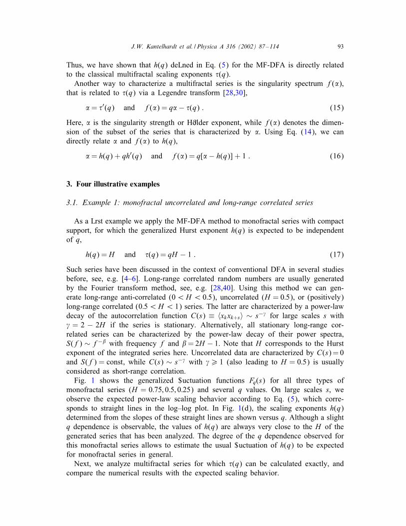
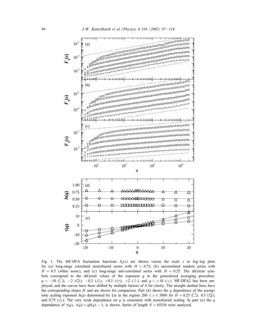
Fig. 1 shows the generalized $uctuation functions Fq(s) for all three types of
monofractal series (H = 0:75; 0:5; 0:25) and several q values. On large scales s, we
observe the expected power-law scaling behavior according to Eq. (5), which corre-
sponds to straight lines in the log–log plot. In Fig. 1(d), the scaling exponents h(q)
determined from the slopes of these straight lines are shown versus q. Although a slight
q dependence is observable, the values of h(q) are always very close to the H of the
generated series that has been analyzed. The degree of the q dependence observed for
this monofractal series allows to estimate the usual $uctuation of h(q) to be expected
for monofractal series in general.
Next, we analyze multifractal series for which �(q) can be calculated exactly, and
compare the numerical results with the expected scaling behavior.
94 J.W. Kantelhardt et al. / Physica A 316 (2002) 87–114
10-4
10-2
(b)
Fq(
s )
0.25
0.50
0.75
1.00 (d)
h (q )
q
10-5
10-3
10-1
(a)
Fq(
s )
101
102 10
310
4
10-3
10-1
(c)
Fq(
s )
s
-20 -10 0 10 20-20
-10
0
10 (e)
τ(q)
Fig. 1. The MF-DFA $uctuation functions Fq(s) are shown versus the scale s in log–log plots
for (a) long-range correlated monofractal series with H = 0:75, (b) uncorrelated random series with
H = 0:5 (white noise), and (c) long-range anti-correlated series with H = 0:25. The diCerent sym-
bols correspond to the diCerent values of the exponent q in the generalized averaging procedure,
q = −10 ( ); −2 (◦); −0:2 (�); +0:2 (�); +2 (�); and q = +10 (+). MF-DFA2 has been em-
ployed, and the curves have been shifted by multiple factors of 4 for clarity. The straight dashed lines have
the corresponding slopes H and are shown for comparison. Part (d) shows the q dependence of the asymp-
totic scaling exponent h(q) determined by Lts in the regime 200¡s¡ 5000 for H = 0:25 ( ); 0:5 (◦);
and 0:75 (�). The very weak dependence on q is consistent with monofractal scaling. In part (e) the q
dependence of �(q); �(q) = qh(q)− 1, is shown. Series of length N = 65536 were analyzed.
J.W. Kantelhardt et al. / Physica A 316 (2002) 87–114 95
3.2. Example 2: binomial multifractal series
In the binomial multifractal model [28–30], a series of N = 2nmax numbers k with
k = 1; : : : ; N is deLned by
xk = an(k−1)(1− a)nmax−n(k−1) ; (18)
where 0:5¡a¡1 is a parameter and n(k) is the number of digits equal to 1 in the binary
representation of the index k, e.g. n(13) = 3, since 13 corresponds to binary 1101.
The scaling exponents �(q) can be calculated straightforwardly. According to
Eqs. (12) and (18) the box probability p2s(�) in the �th segment of size 2s is given by
p2s(�) = ps(2�− 1) + ps(2�) = [(1− a)=a+ 1]ps(2�) = ps(2�)=a :
Thus, according to Eqs. (13) and (18),
Zq(s) =
N=s∑
�=1
[ps(�)]q =
N=2s∑
�=1
[ps(2�− 1)]q + [ps(2�)]q
=
[
(1− a)q
aq+ 1
] N=2s∑
�=1
[ps(2�)]q
= [(1− a)q + aq]
N=2s∑
�=1
[p2s(�)]q = [(1− a)q + aq]Zq(2s)
and according to Eqs. (13) and (14),
�(q) =−ln[aq + (1− a)q]
ln(2); (19)
h(q) =1
q−
ln[aq + (1− a)q]
q ln(2): (20)
Note that �(0) =−1 as required. There is a strong nonlinear dependence of �(q) upon
q, indicating multifractality. The same information is comprised in the q dependence
of h(q). The asymptotic values are h(q) → −ln(a)=ln(2) for q → +∞ and h(q) →−ln(1− a)=ln(2) for q → −∞. They correspond to the scaling behavior of the largest
and weakest $uctuations, respectively. Note that h(q) becomes independent of q in the
asymptotic limit, while �(q) approaches linear q dependences.
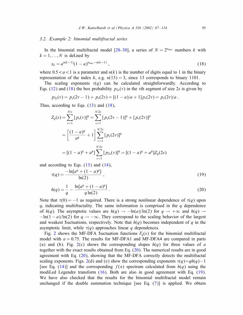
Fig. 2 shows the MF-DFA $uctuation functions Fq(s) for the binomial multifractal
model with a= 0:75. The results for MF-DFA1 and MF-DFA4 are compared in parts
(a) and (b). Fig. 2(c) shows the corresponding slopes h(q) for three values of a
together with the exact results obtained from Eq. (20). The numerical results are in good
agreement with Eq. (20), showing that the MF-DFA correctly detects the multifractal
scaling exponents. Figs. 2(d) and (e) show the corresponding exponents �(q)=qh(q)−1
[see Eq. (14)] and the corresponding f(�) spectrum calculated from h(q) using the
modiLed Legendre transform (16). Both are also in good agreement with Eq. (19).
We have also checked that the results for the binomial multifractal model remain
unchanged if the double summation technique [see Eq. (7)] is applied. We obtain
96 J.W. Kantelhardt et al. / Physica A 316 (2002) 87–114
10-8
10-6
10-4
10-2 (a)
q = 10q = 2q = 0.2q = -0.2q = -2q = -10
Fq(
s )
101
102
103
104
10-9
10-7
10-5
10-3 (b)
Fq(
s )
s
0
1
2
3
4 (c)
a = 0.90, MF-DFA1a = 0.75, MF-DFA1a = 0.75, MF-DFA4a = 0.60, MF-DFA1
h (q )
q-20 -10 0 10 20
-60
-30
0 (d)
τ (q )
0.0 0.5 1.0 1.5 2.00.0
0.5
1.0 (e)
f (α)
α
Fig. 2. The MF-DFA $uctuation functions Fq(s) are shown versus the scale s in log–log plots for the
binomial multifractal model with a = 0:75 (a) for MF-DFA1 and (b) for MF-DFA4. The symbols are the
same as for Fig. 1. The straight dashed lines have the corresponding theoretical slopes h(−10) = 1:90 and
h(+10)=0:515 and are shown for comparison. In part (c) the q dependence of the generalized Hurst exponent
h(q) determined by Lts in the regime 50¡s¡ 500 is shown for MF-DFA1 and a=0:9 (�); a=0:75 (◦);
and a = 0:6 ( ), as well as for MF-DFA4 and a = 0:75 (�). Parts (d) and (e) show the corresponding
exponents �(q) and the corresponding singularity spectrum f(�) for a = 0:75 determined by the modiLed
Legendre transform (16), respectively. The lines are the theoretical values obtained from Eq. (20). Series of
length N = 65536 were analyzed.
J.W. Kantelhardt et al. / Physica A 316 (2002) 87–114 97
slopes h(q) = h(q) + 1 as expected in Eq. (8). Note that there is no need to use this
modiLcation, except if h(q) is close to zero or has negative values.
3.3. Example 3: dyadic random cascade model with log-Poisson distribution
For another independent test of the MF-DFA, we employ an algorithm based on
random cascades on wavelet dyadic trees proposed in Refs. [41,42] (see also [43]).
This algorithm builds a random multifractal series by specifying its discrete wavelet
coeOcients cn;m, deLned recursively,
c1;1 = 1; cn;2m−1 =Wcn−1;m; cn;2m =Wcn−1;m ;
where n=2; : : : ; nmax (with N =2nmax) and m=1; : : : ; 2n−2. The values of W are taken
from a log-Poisson distribution, |W |= exp(P ln !+ �), where P is Poisson distributed
with 〈P〉=". There are three independent parameters, "; !, and �. Inverse wavelet trans-
form is applied to create the multifractal random series xk once the wavelet coeOcients
cn;m are known,
xk =
nmax∑
n=1
2n−1
∑
m=1
cn;m n;m(k) ; (21)
where n;m(k) is a set of wavelets forming an orthonormal wavelet basis. Here, we
employ the Haar wavelets, n;m(k) ≡ 2(n−nmax−1)=2 [2n−nmax−1k −m] with (x) ≡ 1 for
0¡x6 0:5; (x) ≡ −1 for 0:5¡x6 1 and (x) ≡ 0 otherwise. For this model the
multifractal scaling exponents are given by [41,42]
�(q) ="(1− !q)− �q
ln 2− 1 ; (22)
h(q) = ["(1− !q)− �q]=(q ln 2) : (23)
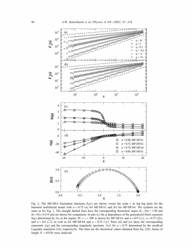
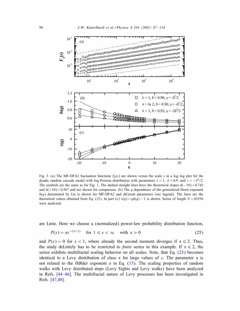
Fig. 3 shows the MF-DFA $uctuation functions Fq(s) for the dyadic random cascade
model. The numerically determined slopes h(q) for three sets of parameters are com-
pared with the exact results obtained from Eq. (23) and the good agreement shows
that the MF-DFA correctly detects the multifractal scaling exponents. Large deviations
occur only for very small moments (q¡ − 10), indicating that the range of q values
should not exceed −10.
3.4. Example 4: uncorrelated multifractal series with power-law distribution
function
The examples discussed in the previous three subsections were based on series in-
volving long-range correlations. In the present example we want to apply the MF-DFA
method to an uncorrelated series, that nevertheless exhibits multifractal scaling behav-
ior due to the broad distribution of its values. We denote by P(x) the probability
density function of the values xk in the series. The distribution P(x) does not aCect
the multifractality of a series on large scales s, if all moments
〈|x|q〉 ≡
∫
∞
−∞
|x|qP(x) dx (24)
98 J.W. Kantelhardt et al. / Physica A 316 (2002) 87–114
101
102
103
104
10-5
10-3
10-1
(a)
Fq(
s )
s
0.6
0.8
1.0
1.2
τ (q )
(b) λ = 1, δ = 0.90, γ = -δ4/2
λ = ln 2, δ = 0.90, γ = -δ4/2
λ = 1, δ = 0.93, γ = -2δ4/5h (
q )
-20 -10 0 10 20-20
-10
0
10(c)
q
Fig. 3. (a) The MF-DFA2 $uctuation functions Fq(s) are shown versus the scale s in a log–log plot for the
dyadic random cascade model with log-Poisson distribution with parameters "= 1; != 0:9, and �=−!4=2.
The symbols are the same as for Fig. 1. The dashed straight lines have the theoretical slopes h(−10)=0:743
and h(+10)=0:567 and are shown for comparison. (b) The q dependence of the generalized Hurst exponent
h(q) determined by Lts is shown for MF-DFA2 and diCerent parameters (see legend). The lines are the
theoretical values obtained from Eq. (23). In part (c) �(q)= qh(q)− 1 is shown. Series of length N =65536
were analyzed.
are Lnite. Here we choose a (normalized) power-law probability distribution function,
P(x) = �x−(�+1) for 16 x¡∞ with �¿ 0 (25)
and P(x) = 0 for x¡ 1, where already the second moment diverges if �6 2. Thus,
the study deLnitely has to be restricted to ?nite series in this example. If �6 2, the
series exhibits multifractal scaling behavior on all scales. Note, that Eq. (25) becomes
identical to a Levy distribution of class � for large values of x. The parameter � is
not related to the H?older exponent � in Eq. (15). The scaling properties of random
walks with Levy distributed steps (Levy $ights and Levy walks) have been analyzed
in Refs. [44–46]. The multifractal nature of Levy processes has been investigated in
Refs. [47,48].
J.W. Kantelhardt et al. / Physica A 316 (2002) 87–114 99
In order to derive the multifractal spectrum, let us consider s uncorrelated random
numbers rk ; k=1; : : : ; s, distributed homogeneously in the interval [0; 1]. Obviously, the
typical value of the minimum of the numbers, rmin(s) ≡ minsk=1rk , will be rmin(s)=1=s.
It can be easily shown that the numbers rk are transformed into numbers xk distributed
according to the power-law probability distribution function (25) by rk → xk = r−1=�k .
Thus, the typical value of the maximum of the xk will be xmax(s) ≡ maxsk=1xk =
[rmin(s)]−1=� = s1=�.
If �6 2, the $uctuations of the proLle Y (i) [Eq. (1)] and the corresponding DFA
variance F2(�; s) [Eq. (2)] will be dominated by the square of the largest value x2max(s)=
s2=� in the segment of s numbers, since the second moment of the distribution (25)
diverges. Now the whole series consists of Ns ≡ int(N=s) segments of length s and not
just of one segment. For some segments �; [F2(�; s)]1=2 is larger than its typical value
xmax(s) = s1=�, since the maximum within the whole series of length N is xmax(N ) =
N 1=�. In order to calculate Fq(s) [Eq. (4)], we need to take into account the whole
distribution Ps(y) of the values y ≡ [F2(�; s)]1=2. Since each of the maxima in the
Ns segments corresponds to an actual number xk and these xk are random numbers
from the power-law distribution (25), it becomes obvious, that the distribution of the
maxima will have the same form, i.e., Ps(y) ∼ P(x = y) for large y. Small values of
y are excluded because of the maximum procedure, but the large xk values are very
likely to be identical to the maxima of the corresponding segments. Since the smallest
maxima for segments of length s are of the order of xmax(s)= s1=�, the lower cutoC for
Ps(y) must be proportional to s1=�. From the normalization condition∫
∞
As1=�Ps(y) dy=1
(with an unimportant prefactor A¡ 1) we get
Ps(y) = A��sy−(�+1) : (26)
Now Fq(s) [Eq. (4)] can be calculated by integration from the minimum value As1=�
of y ≡ [F2(�; s)]1=2 to the maximum value N 1=�. For s�N we obtain
Fq(s)∼
[
∫ N 1=�
As1=�yqPs(y) dy
]1=q
∼ |A�sN q=�−1 − Aqsq=�|1=q ∼
{
s1=q (q¿�)
s1=� (q¡�):
Comparing with Eq. (5), we Lnally get
h(q) ∼
{
1=q (q¿�)
1=� (q6 �): (27)
Note that �(q) follows a linear q dependence, �(q)=q=�−1 for q¡�, while it is equal
to zero for q¿� according to Eq. (14). Hence, the series of uncorrelated power-law
distributed values has rather bi-fractal [48] instead of multifractal properties. Since
h(2)= 12holds exactly for all values of �, it is not possible to recognize the multifrac-
tality due to the broad power-law distribution of the values if only the conventional
DFA is applied. The second moment shows just the uncorrelated behavior of the val-
ues. In a very recent preprint [46] this behavior has been interpreted as a failure of the
100 J.W. Kantelhardt et al. / Physica A 316 (2002) 87–114
101
102
103
104
10-3
10-1
101
103
(a)
Fq(
s )
s
0
1
2α = 0.5
α = 1.0
α = 2.0
(b)
h (q )
q-20 -10 0 10 20
-40
-30
-20
-10
0 (c)
τ(q )
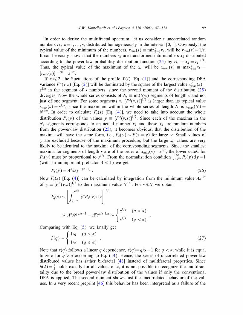
Fig. 4. (a) The modiLed and rescaled MF-DFA3 $uctuation functions Fq(s)=s (corresponding to Fq(s)) are
shown versus the scale s in a log–log plot for a series of independent numbers with a power-law probability
density distribution P(x) ∼ x−(�+1) with �=1. The symbols are the same as for Fig. 1. The straight dashed
lines have the corresponding theoretical slopes h(−10)=1 and h(+10)=0:1 and are shown for comparison.
(b) The q dependence of the generalized Hurst exponent h(q) = h(q)− 1 determined by Lts on large scales
s is shown for MF-DFA3 and � = 0:5 ( ); 1:0 (◦), and 2:0 (�). The lines are the theoretical values
obtained from Eq. (27). In part (c) the corresponding �(q) is shown. The broad distribution of the values
leads to multifractality (bi-fractality) in all three cases. Series of length N = 65536 were analyzed.
DFA and corresponding nondetrending methods for series with a broad distribution,
and another method to determine the exponent 1=� has been proposed. We believe that
a multifractal description with more than one exponent is required to characterize this
kind of series, and thus any method calculating just one exponent will be insuOcient
for a full characterization.
Fig. 4(a) shows the MF-DFA3 $uctuation functions for series of independent random
numbers xk ∈ [1;∞) distributed according to Eq. (25) with � = 1. Since the scaling
J.W. Kantelhardt et al. / Physica A 316 (2002) 87–114 101
exponents h(q) become very close to zero asymptotically for large positive values of
q according to Eq. (27), we must use the modiLed MF-DFA technique involving the
double sum as described in the last paragraph of Section 2.1. Hence, for this techni-
cal reason, Fq(s)=s is calculated instead of Fq(s). The corresponding slopes h(q) − 1
are identical to h(q), see Eq. (8). In Fig. 4(b) the slopes h(q) for series with �=0:5; 1:0,
and 2.0 are compared with the theoretical result Eq. (27), and nice agreement is ob-
served.
4. Comparison of the multifractality for original and shu!ed series
4.1. Distinguishing the two types of multifractality
As already mentioned in the introduction, two diCerent types of multifractality in
time series can be distinguished. Both of them require a multitude of scaling expo-
nents for small and large $uctuations. (i) Multifractality of a time series can be due
to a broad probability density function for the values of the time series, and (ii) mul-
tifractality can also be due to diCerent long-range correlations for small and large
$uctuations.
In general, the example discussed in Section 3.4, the uncorrelated multifractal
series with a power-law probability density function, is of type (i), while the examples
discussed in Sections 3.1–3.3 are of type (ii), where the probability density function
of the values is a regular distribution with Lnite moments. More exactly speaking, the
example of the binomial multifractal series (Section 3.2) can also show multifractal-
ity due to a broad probability density function for the values xk . If the parameter a
is chosen to be very close to one or if very long series are considered, correspond-
ing to large values of nmax, the minimum value in the series, (1 − a)nmax , will be
very small compared with the maximum value anmax [see Eq. (18)]. In this case the
log-binomial probability density function will become broad, approaching a log-normal
form. Since the scaling behavior of uncorrelated log-normal distributed series corre-
sponds to the multifractal scaling behavior observed in the example of uncorrelated
power-law distributed series with � = 2 (see Section 3.4), distribution multifractality
[type (i)] will occur in addition to the correlation multifractality [type (ii)]. For the
series with a= 0:75 and N = 8192 (nmax = 13) considered in Section 3.2, we observe
only type (ii) multifractality caused by long-range correlations.
Now we would like to distinguish between these two types of multifractality. The
most easy way to do so is by analyzing also the corresponding randomly shu6ed
series. In the shu6ing procedure the values are put into random order, and thus all
correlations are destroyed. Hence the shu6ed series from multifractals of type (ii)
will exhibit simple random behavior, hshuf (q)= 0:5, i.e., nonmultifractal scaling like in
Fig. 1(b). For multifractals of type (i), on the contrary, the original h(q) dependence is
not changed, h(q) = hshuf (q), since the multifractality is due to the probability density,
which is not aCected by the shu6ing procedure. If both kinds of multifractality are
present in a given series, the shu6ed series will show weaker multifractality than the
original one.
102 J.W. Kantelhardt et al. / Physica A 316 (2002) 87–114
101
102
103
104
10-6
10-4
10-2
100
s
(b)
F±1
0(s)
/ F
±10sh
uf( s
)
s
101
102
103
10410
-12
10-7
10-2
103
(a)
F±1
0shuf
( s)
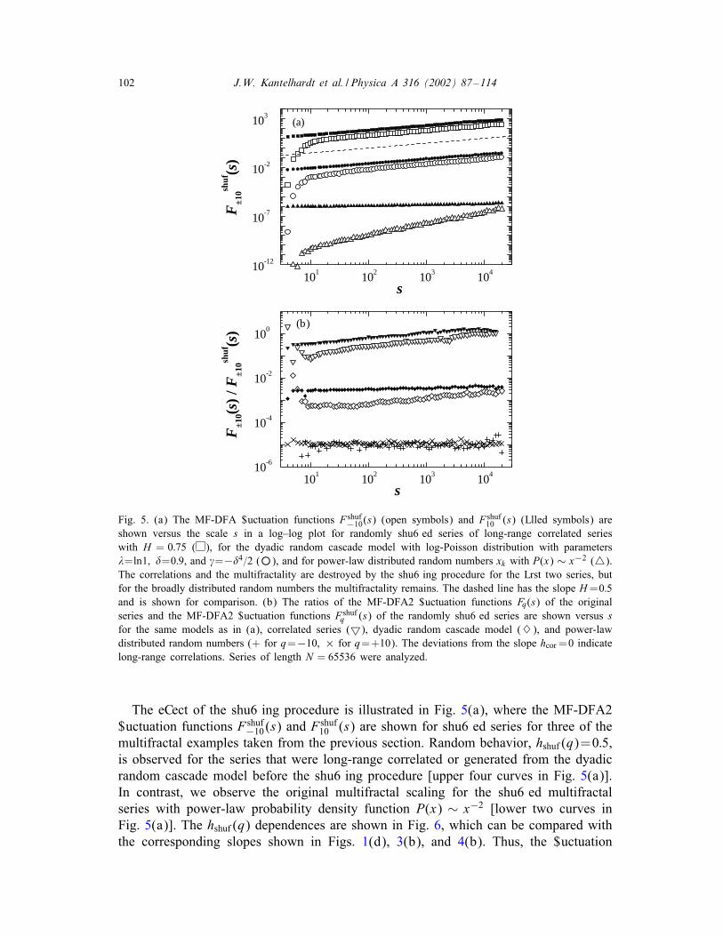
Fig. 5. (a) The MF-DFA $uctuation functions Fshuf−10(s) (open symbols) and Fshuf
10 (s) (Llled symbols) are
shown versus the scale s in a log–log plot for randomly shu6ed series of long-range correlated series
with H = 0:75 ( ), for the dyadic random cascade model with log-Poisson distribution with parameters
"=ln1; !=0:9, and �=−!4=2 (◦), and for power-law distributed random numbers xk with P(x) ∼ x−2 (�).
The correlations and the multifractality are destroyed by the shu6ing procedure for the Lrst two series, but
for the broadly distributed random numbers the multifractality remains. The dashed line has the slope H=0:5
and is shown for comparison. (b) The ratios of the MF-DFA2 $uctuation functions Fq(s) of the original
series and the MF-DFA2 $uctuation functions Fshufq (s) of the randomly shu6ed series are shown versus s
for the same models as in (a), correlated series (�), dyadic random cascade model (�), and power-law
distributed random numbers (+ for q=−10; × for q=+10). The deviations from the slope hcor=0 indicate
long-range correlations. Series of length N = 65536 were analyzed.
The eCect of the shu6ing procedure is illustrated in Fig. 5(a), where the MF-DFA2
$uctuation functions F shuf−10(s) and F shuf
10 (s) are shown for shu6ed series for three of the
multifractal examples taken from the previous section. Random behavior, hshuf (q)=0:5,
is observed for the series that were long-range correlated or generated from the dyadic
random cascade model before the shu6ing procedure [upper four curves in Fig. 5(a)].
In contrast, we observe the original multifractal scaling for the shu6ed multifractal
series with power-law probability density function P(x) ∼ x−2 [lower two curves in
Fig. 5(a)]. The hshuf (q) dependences are shown in Fig. 6, which can be compared with
the corresponding slopes shown in Figs. 1(d), 3(b), and 4(b). Thus, the $uctuation
J.W. Kantelhardt et al. / Physica A 316 (2002) 87–114 103
0.5
1.0
(a)
h shuf
( q)
q-20 -10 0 10 20
-20
-10
0
10(b)
τ shuf
( q)
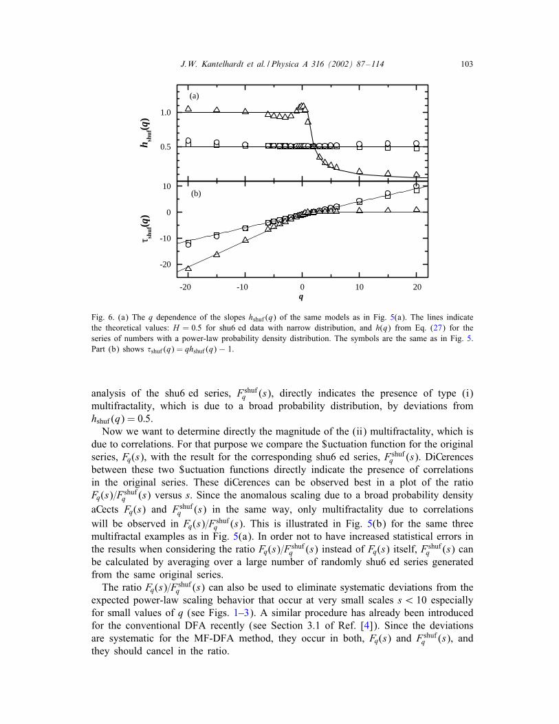
Fig. 6. (a) The q dependence of the slopes hshuf (q) of the same models as in Fig. 5(a). The lines indicate
the theoretical values: H = 0:5 for shu6ed data with narrow distribution, and h(q) from Eq. (27) for the
series of numbers with a power-law probability density distribution. The symbols are the same as in Fig. 5.
Part (b) shows �shuf (q) = qhshuf (q)− 1.
analysis of the shu6ed series, F shufq (s), directly indicates the presence of type (i)
multifractality, which is due to a broad probability distribution, by deviations from
hshuf (q) = 0:5.
Now we want to determine directly the magnitude of the (ii) multifractality, which is
due to correlations. For that purpose we compare the $uctuation function for the original
series, Fq(s), with the result for the corresponding shu6ed series, F shufq (s). DiCerences
between these two $uctuation functions directly indicate the presence of correlations
in the original series. These diCerences can be observed best in a plot of the ratio
Fq(s)=Fshufq (s) versus s. Since the anomalous scaling due to a broad probability density
aCects Fq(s) and F shufq (s) in the same way, only multifractality due to correlations
will be observed in Fq(s)=Fshufq (s). This is illustrated in Fig. 5(b) for the same three
multifractal examples as in Fig. 5(a). In order not to have increased statistical errors in
the results when considering the ratio Fq(s)=Fshufq (s) instead of Fq(s) itself, F
shufq (s) can
be calculated by averaging over a large number of randomly shu6ed series generated
from the same original series.
The ratio Fq(s)=Fshufq (s) can also be used to eliminate systematic deviations from the
expected power-law scaling behavior that occur at very small scales s¡ 10 especially
for small values of q (see Figs. 1–3). A similar procedure has already been introduced
for the conventional DFA recently (see Section 3.1 of Ref. [4]). Since the deviations
are systematic for the MF-DFA method, they occur in both, Fq(s) and F shufq (s), and
they should cancel in the ratio.
104 J.W. Kantelhardt et al. / Physica A 316 (2002) 87–114
The scaling behavior of the ratio is
Fq(s)=Fshufq (s) ∼ sh(q)−hshuf (q) = shcor(q) : (28)
Note that h(q) = hshuf (q) + hcor(q). If only distribution multifractality [type (i)] is
present, h(q) = hshuf (q) depends on q and hcor(q) = 0. On the other hand, deviations
of hcor(q) from zero indicate the presence of correlations, and a q dependence of
hcor(q) indicates correlation multifractality [type (ii)]. If only correlation multifractality
is present, hshuf (q) = 0:5 and h(q) = 0:5 + hcor(q). If both, distribution multifractality
and correlation multifractality are present, both, hshuf (q) and hcor(q) depend on q.
4.2. Signi?cance of the results
In Figs. 1–6 we have shown the results of the MF-DFA for single conLgurations of
long time series. Now we address the signiLcance and accuracy of the MF-DFA results
for short series. How much do the numerically determined exponents h(q) vary from
one conLguration (sample series) to the next, and how close are the average values
to the theoretical values? In other words, how large are the statistical and systematical
deviations of exponents practically determined by the MF-DFA for Lnite series? These
questions are particularly important for short series, where the statistics is poor. If the
values of h(q) are determined inaccurately, the multifractal properties will be reported
inaccurately or even false conclusions on multifractal behavior might be drawn for
monofractal series.
To address the signiLcance and accuracy of the MF-DFA results we generate,
for each of the three examples considered already in Fig. 5, 100 series of length
N = 213 = 8192 and calculate h(−10); h(+10); hshuf (−10), and hshuf (+10) for each
of these series. The corresponding histograms are shown in Fig. 7. For the long-range
power-law correlated series with H = 0:75 we Lnd the following mean values and
standard deviations of the generalized Hurst exponents:
h(−10) = 0:80± 0:03; hshuf (−10) = 0:56± 0:02 ;
h(+10) = 0:72± 0:04; hshuf (+10) = 0:48± 0:02 :
The mean values for the original series are rather close to, but not identical to the the-
oretical value H =0:75. The mean value for q=−10 is about two standard deviations
larger than 0.75, while the value for q = +10 is slightly smaller. These deviations,
though, certainly cannot indicate multifractality, since we analyzed monofractal series.
Instead, they are due to the Lnite, random series, where parts of the series have slightly
larger and slightly smaller scaling exponent just by statistical $uctuations. By consid-
ering negative values of q we focus on the parts with small $uctuations, which are
usually described by a larger scaling exponent. For positive values of q we focus on
the parts with large $uctuations usually described by a smaller value of h. Thus for
short records we always expect a slight diCerence between h(−10) and h(+10) even
if the series are monofractal. If this diCerence is weak, one has to be very careful with
conclusions about multifractality. Practically it is always wise to compare with gener-
ated monofractal series with otherwise similar properties before drawing conclusions
J.W. Kantelhardt et al. / Physica A 316 (2002) 87–114 105
0
20
40
60(a)
original shuffled
No.
of
seri
es
(b)
0.4 0.5 0.6 0.7 0.80
20
40
60(c)
No.
of
seri
es
0.4 0.5 0.6 0.7 0.8
(d)
1.0 1.1 1.2 1.3 1.4 1.50
20
40
60(e)
No.
of
seri
es
h(−10), hshuf
(−10)0.0 0.1 0.2 0.3 0.4
(f )
h(+10), hshuf
(+10)
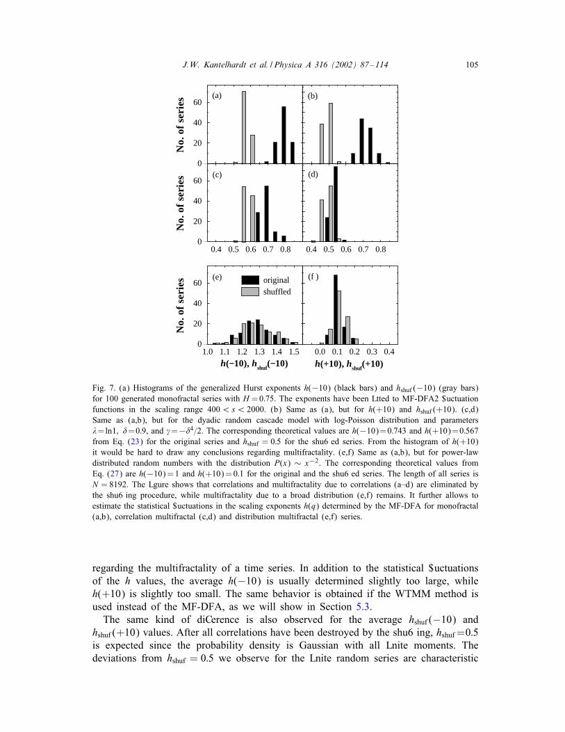
Fig. 7. (a) Histograms of the generalized Hurst exponents h(−10) (black bars) and hshuf (−10) (gray bars)
for 100 generated monofractal series with H =0:75. The exponents have been Ltted to MF-DFA2 $uctuation
functions in the scaling range 400¡s¡ 2000. (b) Same as (a), but for h(+10) and hshuf (+10). (c,d)
Same as (a,b), but for the dyadic random cascade model with log-Poisson distribution and parameters
"=ln1; !=0:9, and �=−!4=2. The corresponding theoretical values are h(−10)=0:743 and h(+10)=0:567
from Eq. (23) for the original series and hshuf = 0:5 for the shu6ed series. From the histogram of h(+10)
it would be hard to draw any conclusions regarding multifractality. (e,f) Same as (a,b), but for power-law
distributed random numbers with the distribution P(x) ∼ x−2. The corresponding theoretical values from
Eq. (27) are h(−10)=1 and h(+10)=0:1 for the original and the shu6ed series. The length of all series is
N = 8192. The Lgure shows that correlations and multifractality due to correlations (a–d) are eliminated by
the shu6ing procedure, while multifractality due to a broad distribution (e,f) remains. It further allows to
estimate the statistical $uctuations in the scaling exponents h(q) determined by the MF-DFA for monofractal
(a,b), correlation multifractal (c,d) and distribution multifractal (e,f) series.
regarding the multifractality of a time series. In addition to the statistical $uctuations
of the h values, the average h(−10) is usually determined slightly too large, while
h(+10) is slightly too small. The same behavior is obtained if the WTMM method is
used instead of the MF-DFA, as we will show in Section 5.3.
The same kind of diCerence is also observed for the average hshuf (−10) and
hshuf (+10) values. After all correlations have been destroyed by the shu6ing, hshuf=0:5
is expected since the probability density is Gaussian with all Lnite moments. The
deviations from hshuf = 0:5 we observe for the Lnite random series are characteristic
106 J.W. Kantelhardt et al. / Physica A 316 (2002) 87–114
for monofractal series of this length (N = 8192). Only for the second moment we
obtain hshuf (2) = 0:5 exactly if a suOcient number of series is considered.
For multifractal series generated from the dyadic random cascade model, Fig. 7(c,d)
shows the histograms of the scaling exponents h(−10); h(+10); hshuf (−10), and
hshuf (+10). Their averages and standard deviations,
h(−10) = 0:69± 0:04; hshuf (−10) = 0:57± 0:02 ;
h(+10) = 0:54± 0:02; hshuf (+10) = 0:48± 0:02
have to be compared with the theoretical values from Eq. (23), h(−10) = 0:743 and
h(+10)=0:567. Surprisingly, the mean h(−10) is smaller than the theoretical value in
this example, but for the mean h(+10) the deviation is similar to the deviation observed
for the monofractal data in the previous example. Again, similar results are obtained
with the WTMM method. For the shu6ed series, the mean generalized Hurst expo-
nents are practically identical to those for the shu6ed monofractal series [the average
hshuf (−10) is larger by half the standard deviation], and both are evidently consistent
with monofractal uncorrelated behavior, h(q)= 0:5, as discussed above. Hence, the se-
ries from the dyadic random cascade model show no signs of distribution multifractality
and are characterized by correlation multifractality only.
The histograms of the scaling exponents for our last example, the power-law dis-
tributed random numbers with P(x) ∼ x−2, are shown in Fig. 7(e,f). The corresponding
mean values and standard deviations
h(−10) = 1:24± 0:09; hshuf (−10) = 1:26± 0:09 ;
h(+10) = 0:11± 0:03; hshuf (+10) = 0:11± 0:04
show obviously no diCerences between original and shu6ed series as expected for
uncorrelated series. This indicates that the multifractality is due to the broad probability
density function only. The values have to be compared with h(−10)=1 and h(+10)=0:1
from Eq. (27). As usual, the average value of h(−10) is too large because we analyzed
short series.
5. Comparison with the WTMM method
5.1. Brief description of the WTMM method
The WTMM method [32–35] is a well-known method to investigate the multifractal
scaling properties of fractal and self-aOne objects in the presence of nonstationari-
ties. For applications, see e.g. [36–39]. It is based upon the wavelet transform with
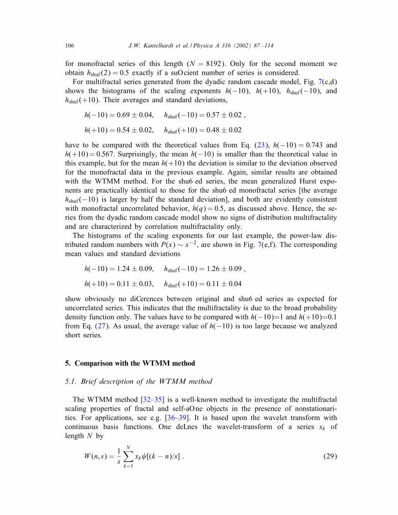
continuous basis functions. One deLnes the wavelet-transform of a series xk of
length N by
W (n; s) =1
s
N∑
k=1
xk [(k − n)=s] : (29)
J.W. Kantelhardt et al. / Physica A 316 (2002) 87–114 107
Note that in this case the series xk are analyzed directly instead of the proLle Y (i)
deLned in Eq. (1). Here, the function (x) is the analyzing wavelet and s is, as above,
the scale parameter. The wavelet is chosen orthogonal to the possible trend. If the trend
can be represented by a polynomial, a good choice for (x) is the mth derivative of
a Gaussian, (m)(x) = dm(e−x2=2)=dxm. This way, the transform eliminates trends up to
(m− 1)th order.
Now, instead of averaging over all values of W (n; s), one averages, within the
modulo-maxima method, only the local maxima of |W (n; s)|. First, one determines
for a given scale s, the positions ni of the local maxima of |W (n; s)| as function of n,
so that |W (ni−1; s)|¡ |W (ni ; s)|¿ |W (ni+1; s)| for i=1; : : : ; imax. Then one sums up
the qth power of these maxima,
Z(q; s) =
imax∑
i=1
|W (ni ; s)|q : (30)
The reason for this maxima procedure is that the absolute wavelet coeOcients |W (n; s)|can become arbitrarily small. The analyzing wavelet (x) must always have positive
values for some x and negative values for other x, since it has to be orthogonal to
possible constant trends. Hence there are always positive and negative terms in the
sum (29), and these terms might cancel. If that happens, |W (n; s)| can become close
to zero. Since such small terms would spoil the calculation of negative moments in
Eq. (30), they have to be eliminated by the maxima procedure. In the MF-DFA,
the calculation of the variances F2(�; s) in Eq. (2), i.e., the deviations from the
Lts, involves only positive terms under the summation. The variances cannot become
arbitrarily small, and hence no maximum procedure is required for series with compact
support.
In addition, the MF-DFA variances will always increase if the segment length s is
increased, because the Lt will always be worse for a longer segment. In the WTMM
method, in contrast, the absolute wavelet coeOcients |W (n; s)| need not increase with
increasing scale s, even if only the local maxima are considered. The values |W (n; s)|might become smaller for increasing s since just more (positive and negative) terms
are included in the summation (29), and these might cancel even better. Thus, an
additional supremum procedure has been introduced in the WTMM method in order to
keep the dependence of Z(q; s) on s monotonous: If, for a given scale s, a maximum
at a certain position ni happens to be smaller than a maximum at n′i ≈ ni for a lower
scale s′¡s, then W (ni ; s) is replaced by W (n′i ; s′) in Eq. (30). There is no need for
such a supremum procedure in the MF-DFA.
Often, scaling behavior is observed for Z(q; s), and scaling exponents �(q) can be
deLned that describe how Z(q; s) scales with s,
Z(q; s) ∼ s�(q) : (31)
The exponents �(q) characterize the multifractal properties of the series under investi-
gation, and theoretically they are identical to the �(q) deLned in Eq. (13) [32–35] and
related to h(q) in Eq. (14).
108 J.W. Kantelhardt et al. / Physica A 316 (2002) 87–114
5.2. Examples for series with nonstationarities
Since the WTMM method has been developed to analyze multifractal series with
nonstationarities, such as trends or spikes, we will compare its performance with the
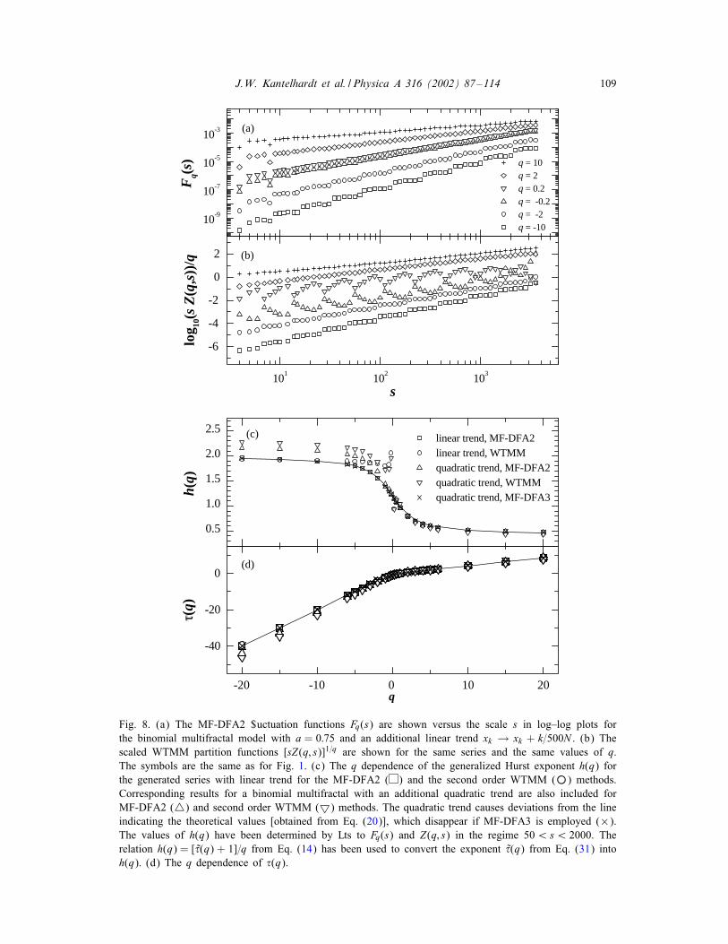
performance of the MF-DFA for such nonstationary series. In Fig. 8 the MF-DFA $uc-
tuation function Fq(s) and its scaling behavior are compared with the rescaled WTMM
partition sum Z(q; s) for the binomial multifractal described in Section 3.2. To test
the detrending capability of both methods, we have added linear as well as quadratic
trends to the generated multifractal series. The trends are removed by both methods, if
a suOciently high order of detrending is employed. The deviations from the theoretical
values of the scaling exponents h(q) [given by Eq. (20)] are of similar size for the
MF-DFA and the WTMM method. Thus, the detrending capability and the accuracy
of both methods are equivalent.
We also obtain similar results for a monofractal long-range correlated series with
additional spikes (outliers) that consist of large random numbers and replace a small
fraction of the original series in randomly chosen positions. The spikes lead to mul-
tifractality on small scales s, while the series remains monofractal on large scales.
Thus, the eCects of the spikes are eliminated neither by the WTMM method nor by
the MF-DFA, but both methods again give rather equivalent results.
5.3. Signi?cance of the results
The last problem we address is a comparison of the signiLcance of the results ob-
tained by the MF-DFA and the WTMM method. The signiLcance of the MF-DFA
results has already been discussed in detail in Section 4.2. Here we will compare the
signiLcance of both methods for short and long series.
We begin with the signiLcance of the results for random series involving nei-
ther correlations nor a broad distribution [as in Fig. 1(b)]. Fig. 9 shows the dis-
tribution of the multifractal Hurst exponents h(−10) and h(+10) calculated by the
MF-DFA as well as by the WTMM using the relation h(q) = [�(q) + 1]=q based on
Eq. (14). Similar to the results presented in Fig. 7, we have analyzed 100 gener-
ated series of uncorrelated random numbers. In addition, we compare the results for
the (relatively short) series length N = 213 = 8192 and for N = 216 = 65532. Ide-
ally, both, h(−10) and h(+10), should be equal to the Hurst exponent of the uncor-
related monofractal series, H = 0:5. The histograms show that similar deviations as
well as remarkable $uctuations of the exponents occur for both methods, as discussed
in Section 4.2 for the MF-DFA. We Lnd the following mean values and standard
deviations,
h(−10) =
0:55± 0:03 for MF-DFA (N = 8k)
0:52± 0:02 for MF-DFA (N = 64k)
0:58± 0:05 for WTMM (N = 8k)
0:56± 0:03 for WTMM (N = 64k)
J.W. Kantelhardt et al. / Physica A 316 (2002) 87–114 109
10-9
10-7
10-5
10-3 (a)
q = 10q = 2q = 0.2q = -0.2q = -2q = -10
Fq(
s )
101
102
103
-6
-4
-2
0
2 (b)
log 10
(s Z
(q,s
))/q
s
0.5
1.0
1.5
2.0
2.5 (c) linear trend, MF-DFA2 linear trend, WTMM quadratic trend, MF-DFA2 quadratic trend, WTMM quadratic trend, MF-DFA3h (
q )
q-20 -10 0 10 20
-40
-20
0(d)
τ (q )
Fig. 8. (a) The MF-DFA2 $uctuation functions Fq(s) are shown versus the scale s in log–log plots for
the binomial multifractal model with a = 0:75 and an additional linear trend xk → xk + k=500N . (b) The
scaled WTMM partition functions [sZ(q; s)]1=q are shown for the same series and the same values of q.
The symbols are the same as for Fig. 1. (c) The q dependence of the generalized Hurst exponent h(q) for
the generated series with linear trend for the MF-DFA2 ( ) and the second order WTMM (◦) methods.
Corresponding results for a binomial multifractal with an additional quadratic trend are also included for
MF-DFA2 (�) and second order WTMM (�) methods. The quadratic trend causes deviations from the line
indicating the theoretical values [obtained from Eq. (20)], which disappear if MF-DFA3 is employed (×).
The values of h(q) have been determined by Lts to Fq(s) and Z(q; s) in the regime 50¡s¡ 2000. The
relation h(q) = [�(q) + 1]=q from Eq. (14) has been used to convert the exponent �(q) from Eq. (31) into
h(q). (d) The q dependence of �(q).
110 J.W. Kantelhardt et al. / Physica A 316 (2002) 87–114
0
20
40
60 (a)
MF-DFA WTMM
No.
of
seri
es
(b)
0.5 0.6 0.70
20
40
60 (c)N
o. o
f se
ries
h(−10)0.4 0.5 0.6
(d)
h(+10)
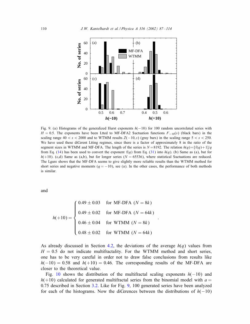
Fig. 9. (a) Histograms of the generalized Hurst exponents h(−10) for 100 random uncorrelated series with
H = 0:5. The exponents have been Ltted to MF-DFA2 $uctuation functions F−10(s) (black bars) in the
scaling range 40¡s¡ 2000 and to WTMM results Z(−10; s) (gray bars) in the scaling range 5¡s¡ 250.
We have used these diCerent Ltting regimes, since there is a factor of approximately 8 in the ratio of the
segment sizes in WTMM and MF-DFA. The length of the series is N=8192. The relation h(q)=[�(q)+1]=q
from Eq. (14) has been used to convert the exponent �(q) from Eq. (31) into h(q). (b) Same as (a), but for
h(+10). (c,d) Same as (a,b), but for longer series (N = 65536), where statistical $uctuations are reduced.
The Lgure shows that the MF-DFA seems to give slightly more reliable results than the WTMM method for
short series and negative moments (q=−10), see (a). In the other cases, the performance of both methods
is similar.
and
h(+10) =
0:49± 0:03 for MF-DFA (N = 8k)
0:49± 0:02 for MF-DFA (N = 64k)
0:46± 0:04 for WTMM (N = 8k)
0:48± 0:02 for WTMM (N = 64k)
:
As already discussed in Section 4.2, the deviations of the average h(q) values from
H = 0:5 do not indicate multifractality. For the WTMM method and short series,
one has to be very careful in order not to draw false conclusions from results like
h(−10) = 0:58 and h(+10) = 0:46. The corresponding results of the MF-DFA are
closer to the theoretical value.
Fig. 10 shows the distribution of the multifractal scaling exponents h(−10) and
h(+10) calculated for generated multifractal series from the binomial model with a=
0:75 described in Section 3.2. Like for Fig. 9, 100 generated series have been analyzed
for each of the histograms. Now the diCerences between the distributions of h(−10)
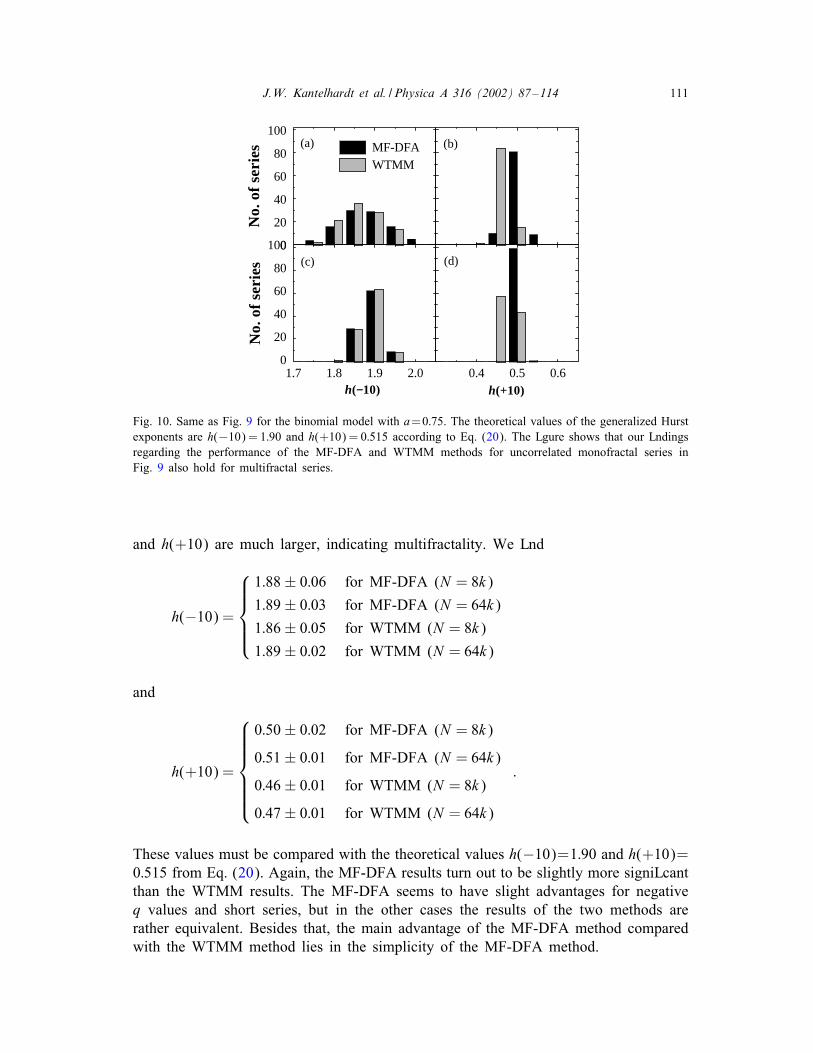
J.W. Kantelhardt et al. / Physica A 316 (2002) 87–114 111
0
20
40
60
80
100(a) MF-DFA
WTMM
No.
of
seri
es
(b)
1.7 1.8 1.9 2.00
20
40
60
80
100(c)
No.
of
seri
es
h(−10)0.4 0.5 0.6
(d)
h(+10)
Fig. 10. Same as Fig. 9 for the binomial model with a=0:75. The theoretical values of the generalized Hurst
exponents are h(−10) = 1:90 and h(+10) = 0:515 according to Eq. (20). The Lgure shows that our Lndings
regarding the performance of the MF-DFA and WTMM methods for uncorrelated monofractal series in
Fig. 9 also hold for multifractal series.
and h(+10) are much larger, indicating multifractality. We Lnd
h(−10) =
1:88± 0:06 for MF-DFA (N = 8k)
1:89± 0:03 for MF-DFA (N = 64k)
1:86± 0:05 for WTMM (N = 8k)
1:89± 0:02 for WTMM (N = 64k)
and
h(+10) =
0:50± 0:02 for MF-DFA (N = 8k)
0:51± 0:01 for MF-DFA (N = 64k)
0:46± 0:01 for WTMM (N = 8k)
0:47± 0:01 for WTMM (N = 64k)
:
These values must be compared with the theoretical values h(−10)=1:90 and h(+10)=
0:515 from Eq. (20). Again, the MF-DFA results turn out to be slightly more signiLcant
than the WTMM results. The MF-DFA seems to have slight advantages for negative
q values and short series, but in the other cases the results of the two methods are
rather equivalent. Besides that, the main advantage of the MF-DFA method compared
with the WTMM method lies in the simplicity of the MF-DFA method.
112 J.W. Kantelhardt et al. / Physica A 316 (2002) 87–114
6. Conclusion
We have generalized the DFA, widely recognized as a method to analyze the (mono-)
fractal scaling properties of nonstationary time series. The MF-DFA method allows
a reliable multifractal characterization of multifractal nonstationary time series. The
implementation of the new method is not more diOcult than that of the conventional
DFA, since just one additional step, a q dependent averaging procedure, is required. We
have shown for stationary signals that the generalized (multifractal) scaling exponent
h(q) for series with compact support is directly related to the exponent �(q) of the
standard partition function-based multifractal formalism. Further, we have shown in
several examples that the MF-DFA method can reliably determine the multifractal
scaling behavior of the time series, similar to the WTMM method which is a more
complicated procedure for this purpose. For short series and negative moments, the
signiLcance of the results for the MF-DFA seems to be slightly better than for the
WTMM method.
Contrary to the WTMM method, the MF-DFA method as described in Section 2.1
requires series of compact support, because the averaging procedure in Eq. (4) will
only work if F2(�; s)¿ 0 for all segments �. Although most time series will fulLll
this prerequisite, it can be overcome by a modiLcation of the MF-DFA technique in
order to analyze data with fractal support: We restrict the sum in Eq. (4) to the local
maxima, i.e., to those terms F2(�; s) that are larger than the terms F2(� − 1; s) and
F2(� + 1; s) for the neighboring segments. By this restriction all terms F2(�; s) that
are zero or very close to zero will be disregarded, and series with fractal support
can be analyzed. The procedure reminds slightly of the modulus maxima procedure
in the WTMM method (see Section 5.1). There is no need, though, to employ a
continuously sliding window or to calculate the supremum over all lower scales for
the MF-DFA, since the variances F2(�; s), which are determined by the deviations
from the Lt, will always increase when the segment size s is increased. In the maxima
MF-DFA procedure the generalized Hurst exponent h(q) deLned in Eq. (5) will depend
on q and even diverge for q → 0 for monofractal series with noncompact support. Thus,
it is more appropriate to consider the scaling exponent �(q), calculating∑
F2(�−1; s)¡F2(�; s)¿F2(�+1; s)
[F2(�; s)]q=2 ∼ s�(q) : (32)
This extended MF-DFA procedure will also be applicable for data with fractal support.
In our future work we will apply the MF-DFA method to a range of physiological
and meteorological data.
Acknowledgements
We would like to thank Yosef Ashkenazy for useful discussions and the German
Academic Exchange Service (DAAD), the Deutsche Forschungsgemeinschaft (DFG),
the German Israeli Foundation (GIF), the Minerva Foundation, and the NIH/National
Center for Research Resources for Lnancial support.
J.W. Kantelhardt et al. / Physica A 316 (2002) 87–114 113
References
[1] C.-K. Peng, S.V. Buldyrev, S. Havlin, M. Simons, H.E. Stanley, A.L. Goldberger, Phys. Rev. E 49
(1994) 1685.
[2] S.M. Ossadnik, S.B. Buldyrev, A.L. Goldberger, S. Havlin, R.N. Mantegna, C.-K. Peng, M. Simons,
H.E. Stanley, Biophys. J. 67 (1994) 64.
[3] M.S. Taqqu, V. Teverovsky, W. Willinger, Fractals 3 (1995) 785.
[4] J.W. Kantelhardt, E. Koscielny-Bunde, H.H.A. Rego, S. Havlin, A. Bunde, Physica A 295 (2001) 441.
[5] K. Hu, P.Ch. Ivanov, Z. Chen, P. Carpena, H.E. Stanley, Phys. Rev. E 64 (2001) 011114.
[6] Z. Chen, P.Ch. Ivanov, K. Hu, H.E. Stanley, Phys. Rev. E 65 (2002) 041107.
[7] S.V. Buldyrev, A.L. Goldberger, S. Havlin, R.N. Mantegna, M.E. Matsa, C.-K. Peng, M. Simons,
H.E. Stanley, Phys. Rev. E 51 (1995) 5084.
[8] S.V. Buldyrev, N.V. Dokholyan, A.L. Goldberger, S. Havlin, C.-K. Peng, H.E. Stanley,
G.M. Viswanathan, Physica A 249 (1998) 430.
[9] C.-K. Peng, S. Havlin, H.E. Stanley, A.L. Goldberger, Chaos 5 (1995) 82.
[10] P.Ch. Ivanov, A. Bunde, L.A.N. Amaral, S. Havlin, J. Fritsch-Yelle, R.M. Baevsky, H.E. Stanley,
A.L. Goldberger, Europhys. Lett. 48 (1999) 594.
[11] Y. Ashkenazy, M. Lewkowicz, J. Levitan, S. Havlin, K. Saermark, H. Moelgaard, P.E.B. Thomsen,
M. Moller, U. Hintze, H.V. Huikuri, Europhys. Lett. 53 (2001) 709.
[12] Y. Ashkenazy, P.Ch. Ivanov, S. Havlin, C.-K. Peng, A.L. Goldberger, H.E. Stanley, Phys. Rev. Lett.
86 (2001) 1900.
[13] A. Bunde, S. Havlin, J.W. Kantelhardt, T. Penzel, J.-H. Peter, K. Voigt, Phys. Rev. Lett. 85 (2000)
3736.
[14] S. Blesic, S. Milosevic, D. Stratimirovic, M. Ljubisavljevic, Physica A 268 (1999) 275.
[15] S. Bahar, J.W. Kantelhardt, A. Neiman, H.H.A. Rego, D.F. Russell, L. Wilkens, A. Bunde, F. Moss,
Europhys. Lett. 56 (2001) 454.
[16] J.M. HausdorC, S.L. Mitchell, R. Firtion, C.-K. Peng, M.E. Cudkowicz, J.Y. Wei, A.L. Goldberger,
J. Appl. Physiol. 82 (1997) 262.
[17] E. Koscielny-Bunde, A. Bunde, S. Havlin, H.E. Roman, Y. Goldreich, H.-J. Schellnhuber, Phys. Rev.
Lett. 81 (1998) 729.
[18] K. Ivanova, M. Ausloos, Physica A 274 (1999) 349.
[19] P. Talkner, R.O. Weber, Phys. Rev. E 62 (2000) 150.
[20] K. Ivanova, M. Ausloos, E.E. Clothiaux, T.P. Ackerman, Europhys. Lett. 52 (2000) 40.
[21] B.D. Malamud, D.L. Turcotte, J. Stat. Plan. Infer. 80 (1999) 173.
[22] C.L. Alados, M.A. HuCman, Ethnology 106 (2000) 105.
[23] R.N. Mantegna, H.E. Stanley, An Introduction to Econophysics, Cambridge University Press, Cambridge,
2000.
[24] Y. Liu, P. Gopikrishnan, P. Cizeau, M. Meyer, C.-K. Peng, H.E. Stanley, Phys. Rev. E 60 (1999) 1390.
[25] N. Vandewalle, M. Ausloos, P. Boveroux, Physica A 269 (1999) 170.
[26] J.W. Kantelhardt, R. Berkovits, S. Havlin, A. Bunde, Physica A 266 (1999) 461.
[27] N. Vandewalle, M. Ausloos, M. Houssa, P.W. Mertens, M.M. Heyns, Appl. Phys. Lett. 74 (1999) 1579.
[28] J. Feder, Fractals, Plenum Press, New York, 1988.
[29] A.-L. BarabWasi, T. Vicsek, Phys. Rev. A 44 (1991) 2730.
[30] H.-O. Peitgen, H. J?urgens, D. Saupe, Chaos and Fractals, Springer, New York, 1992 (Appendix B).
[31] E. Bacry, J. Delour, J.F. Muzy, Phys. Rev. E 64 (2001) 026103.
[32] J.F. Muzy, E. Bacry, A. Arneodo, Phys. Rev. Lett. 67 (1991) 3515.
[33] J.F. Muzy, E. Bacry, A. Arneodo, Int. J. Bifurcat. Chaos 4 (1994) 245.
[34] A. Arneodo, E. Bacry, P.V. Graves, J.F. Muzy, Phys. Rev. Lett. 74 (1995) 3293.
[35] A. Arneodo, et al., in: A. Bunde, J. Kropp, H.-J. Schellnhuber (Eds.), The Science of Disaster: Climate
Disruptions, Market Crashes, and Heart Attacks, Springer, Berlin, 2002, pp. 27–102.
[36] P.Ch. Ivanov, L.A.N. Amaral, A.L. Goldberger, S. Havlin, M.G. Rosenblum, Z.R. Struzik, H.E. Stanley,
Nature 399 (1999) 461.
[37] L.A.N. Amaral, P.Ch. Ivanov, N. Aoyagi, I. Hidaka, S. Tomono, A.L. Goldberger, H.E. Stanley,
Y. Yamamoto, Phys. Rev. Lett. 86 (2001) 6026.
114 J.W. Kantelhardt et al. / Physica A 316 (2002) 87–114
[38] A. Arneodo, N. Decoster, S.G. Roux, Eur. Phys. J. B 15 (2000) 567, 739, and 765.
[39] A. Silchenko, C.K. Hu, Phys. Rev. E 63 (2001) 041105.
[40] H.A. Makse, S. Havlin, M. Schwartz, H.E. Stanley, Phys. Rev. E 53 (1996) 5445.
[41] A. Arneodo, E. Bacry, J.F. Muzy, J. Math. Phys. 39 (1998) 4142.
[42] A. Arneodo, S. Manneville, J.F. Muzy, Europhys. J. B 1 (1998) 129.
[43] Y. Ashkenazy, S. Havlin. P.Ch. Ivanov, C.K. Peng, V. Schulte-Frohlinde, H.E. Stanley, unpublished
(cond-mat/0111396).
[44] M.F. Shlesinger, B.J. West, J. Klafter, Phys. Rev. Lett. 58 (1987) 1100.
[45] S. Havlin, Y. Ben Avraham, DiCusion and Reactions in Fractals and Disordered Systems, Cambridge
University Press, Cambridge, 2000, p. 48, and references therein.
[46] N. Scafetta, P. Grigolini, unpublished (cond-mat/0202008).
[47] S. JaCard, Probab. Theory Relat. 114 (1999) 207.
[48] H. Nakao, Phys. Lett. A 266 (2000) 282.
Related Documents


![DETRENDED TOPOGRAPHIC DATA OF THE SOUTH … · surface, detailing the interior composition [3, 4], ... Conclusions: Detrended topographic data provide a quantifiable method for enhancing](https://static.cupdf.com/doc/110x72/5adb1d647f8b9a6d318dabfc/detrended-topographic-data-of-the-south-detailing-the-interior-composition-3.jpg)