Multibeam echosounder observations reveal interactions ...

MARINE ECOLOGY PROGRESS SERIESMar Ecol Prog Ser

Vol. 378: 199–209, 2009doi: 10.3354/meps07795

Published March 12

INTRODUCTION

Antarctic krill play a pivotal role in the SouthernOcean ecosystem (Mangel & Nicol 2000, Atkinson et al.2001) but are difficult to sample because of their ex-tremely patchy distribution: much krill biomass is con-tained in a few high-density swarms (Brierley et al.1999, Hofmann et al. 2004) that may be undersampledduring surveys with conventional narrow-beam echo-sounders along widely spaced transects. Managing krill

resources, particularly in an ecosystem context, re-quires data on the patterns of temporal and spatial in-teractions between krill and the many predators thatdepend on them, but efforts to gather requisite data atsea have been hampered because of major difficultiesin sampling krill over appropriate scales (Logerwell etal. 1998, Hewitt & Demer 2000). Attempts to link thedistributions of krill and their predators from observa-tions along survey transects may have been unsuccess-ful because the downward-looking echosounders used

© Inter-Research 2009 · www.int-res.com*Email: [email protected]

Multibeam echosounder observations revealinteractions between Antarctic krill and

air-breathing predators

Martin J. Cox1,*, David A. Demer2, Joseph D. Warren3, George R. Cutter2, Andrew S. Brierley1

1Pelagic Ecology Research Group, Gatty Marine Laboratory, University of St. Andrews, Fife KY16 8LB, UK2Advanced Survey Technology Program, Southwest Fisheries Science Center, 8604 La Jolla Shores Drive, La Jolla,

California 92037, USA3School of Marine and Atmospheric Sciences, Stony Brook University, 239 Montauk Highway, Southampton,

New York 11968, USA

ABSTRACT: A multibeam echosounder (MBE) was deployed on an inflatable boat (length = 5.5 m) toobserve swarms of Antarctic krill Euphausia superba in the nearshore environment off LivingstonIsland, South Shetland Islands, Antarctica. Visual observations of air-breathing predators, includingpenguins and fur seals, were made from the boat at the same time. MBEs extend the 2-dimensionalacoustic observations that can be made with conventional vertical echosounders to 3 dimensions,enabling direct observation of the surface areas and volumes of entire krill swarms. Krill swarmsexhibited a wide range of various size metrics (e.g. height, length and width) but only a narrow rangeof surface-area-to-volume ratios or ‘roughnesses’, suggesting that krill adopt a consistent groupbehavior to maintain swarm shape. The variation in R was investigated using generalized additivemodels (GAMs). GAMs indicated that the presence of air-breathing predators influenced swarmshape (R decreased as the range to predators decreased, and the swarms became more spherical), asdid swarm nearest-neighbor distance (R decreased with increasing distance) and swarm position inthe water column (R decreased in the upper 70% of the water column). Therefore, swarm shapeappears to be influenced by a combination of behavioral responses to predator presence and environ-mental variables. MBEs have the potential to contribute much to studies of krill, and can provide datato improve our understanding of the behavior of krill in situ.

KEY WORDS: Antarctic krill · Euphausia superba · Predator–prey interactions · Multibeamechosounder · Swarm morphology · Livingston Island

Resale or republication not permitted without written consent of the publisher

OPENPEN ACCESSCCESS

Mar Ecol Prog Ser 378: 199–209, 2009

to routinely estimate krill abundance (Hewitt et al.2004), fail to detect krill swarms just off the survey trackline. Research by Zamon et al. (1996), using a small-scale (1852 m2), line-transect grid (transect spacingca. 300 m) suggests that predators observed visually inthe vicinity of the research vessel may be feeding uponthese undetected krill swarms, leading to spatial mis-match in the krill–predator observations. Conventionalsingle-beam echosounders (SBEs) sample only a nar-row cone of water (typically 7°) beneath the researchvessel. For a vessel with a draft of 5 m this provides awindow of observation just 3 m wide at 30 m depth:visual observations of predators on the other hand mayspan tens or hundreds of meters either side of the ves-sel. Multibeam echosounders (MBEs) sample a widerswath (e.g. 90 to 120°) and extend greatly the observa-tion to the sides of the survey track: for example in100 m of water a 120° swath may sample within a rangeof 173 m to either side of the survey track. Thus, the2-dimensional (2D) view provided by SBEs is effec-tively extended into 3 dimensions (3D; Gerlotto et al.1999) by MBEs, offering the potential to examine fine-scale interactions (sensu Zamon et al. 1996).

The sampling volume differences between SBEs andMBEs arise due to the way each instrument samplesthe water column. The 1-dimensional observationsfrom an SBE of the acoustic mean volume backscatter-ing strength (Sv, logarithmic measure, units dB) down

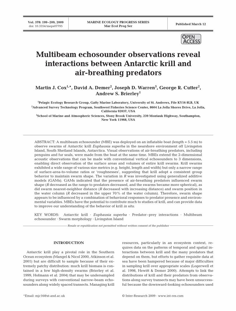
the water column are combined over adjacent pings (atransmit and receive cycle; a typical ping rate is 1 s–1)and are used to build up a 2D matrix from a narrowslice of the water column along the survey track (Reid& Simmonds 1993). In contrast, a single ping from anMBE (Fig. 1) samples a swath through the water col-umn across the survey track. Each swath is made up ofobservations from multiple acoustic beams that radiatefrom a central point, with the position of each Sv obser-vation within a swath being described in 2D in terms ofa range and bearing from the origin. By combiningsuccessive swaths, a 3D acoustic image of the watercolumn along and to either side of the survey track canbe created.

MBEs have been used to investigate predator–preyinteractions, for example between Atlantic puffins Fra-tercula arctica and herring Clupea harengus (Axelsenet al. 2001). Gerlotto & Paramo (2003) used MBEs toinvestigate the geometry of pelagic aggregations ofthe clupeid Sardinella aurita. MBEs have also beenused to study the 3D structure and vessel avoidancebehavior of anchovy Engraulis ringens and commonsardine Strangomera bentincki schools (Gerlotto et al.2004), and to assess the 3D school structure of clupeidsS. aurita and Sardinops sagax (Paramo et al. 2007).

The objectives of the present study were to (1)examine the utility of an MBE for observations ofAntarctic krill, and (2) use an MBE to improve our

200

2

1

43

Sv (dB)

23.0

53.0

26.0

29.0

32.0

35.0

38.0

41.0

44.0

47.0

50.0

Fig. 1. A single multibeam echosounder (MBE) ping (range = 200 m), showing acoustic mean volume backscattering strength(Sv, dB, uncalibrated) Sv values from 23 to 53 dB. Numbers identify the following features: 1 = the MBE seabed profile; 2 = the

effective sampling volume; 3 = a krill swarm; and 4 = seabed side lobe detections that limited the sampling volume

Cox et al.: Multibeam echosounder studies of Antarctic krill

understanding of interactions between krill andpredators at the small to mesoscale (tens to thousandsof meters). The acoustic reflectivity or target strength(logarithmic measure, units dB) of krill is approxi-mately 1000 times less than that of the fish that havepreviously been observed using MBEs. For example,at 120 kHz, the target strength of a 38 mm long krillis approximately –77 dB (Demer & Conti 2005), com-pared to about –43 dB for a 21 cm long herring(Gorska & Ona 2003). Although theory indicates thatkrill should be detectable with an MBE, the firstobjective was to achieve a practical demonstration ofkrill observations in the Southern Ocean. The secondobjective involved using the large sampling volumeand the 3D imaging capabilities of the MBE to exam-ine possible relationships between krill swarms andpredators, to determine for example if predators for-aged in regions with an elevated number of krillswarms. To achieve these objectives we evaluatedthe utility of an MBE for studying at-sea predator–prey interactions by comparing MBE and SBE obser-vations. In addition, using MBE and predator observa-tions in a generalized additive modeling (GAM)framework, we estimated the spatial scales at whichair-breathing krill predators and krill interacted, andinvestigated the influence predators may have had onkrill swarm shape.

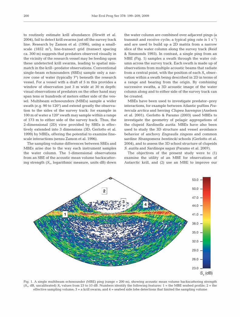
The observations reported here were made nearCape Shirreff in the vicinity of Livingston Island(62.6° S, 60.3° W), South Shetland Islands, Antarctica(Fig. 2). The reproductive season of marine land-breeding animals, such as penguins and fur seals, atthe South Shetland Islands lasts from November toMarch (Hewitt et al. 2003). During this time, largechanges in krill wet mass density (g m–2) year-to-yearhave been recorded (e.g. varying from 1 to 60 g m–2

during 1992 to 2006; Hewitt & Demer 1994, Hewitt etal. 2004, Reiss et al. 2008). Moreover, years when land-based predators exhibited reduced reproductive suc-cess coincided with years of low krill density (Hewitt etal. 2003).

During the reproductive season, the duration offoraging trips made by land-based predators are con-strained by rearing and feeding requirements (i.e.most foraging effort is close to land by ‘central place’foragers). It is therefore important to assess the den-sity and spatial distribution of krill, and their physicaloceanographic environment, in the nearshore areasurrounding penguin and seal colonies, such as atCape Shirreff. This information is required for ecosys-tem studies and also as a component of the holisticecosystem approach to managing exploitation of liv-ing marine resources such as krill in a way that doesnot adversely affect dependent predators (Constableet al. 2000).

MATERIALS AND METHODS

An inflatable boat, RV ‘Roald’ (Mark V Zodiac, length5.5 m), was deployed in the vicinity of Cape Shirreff,from 2 to 9 February 2006 (Fig. 2). RV ‘Roald’ (Fig. 3)was equipped with a Simrad Mesotech SM20, 200 kHzMBE that was used to conduct a high-resolution bathy-metry survey (100% seabed coverage; depth accuracy± 1 m, 95% CI) and to undertake simultaneous watercolumn sampling to observe krill swarms acoustically.Between 4 and 8 February 2006, RV ‘Roald’ followed asystematic line-transect plan (Fig. 2). Each transect waseither 2.5 or 3.5 km long, and line spacing was 120 m.

Multibeam equipment and data description. TheSM20 was configured with an 80-element array tocreate 128 receive beams, each with a 1.5° across-trackand 20° along-track beam width, creating a totalacross-track swath width of 120°. An orthogonallymounted external transmit or profiling transducer wasused to reduce the along-track beam width from 20° to1.5°, which improved the precision of locating targetsin the water column and reduced between-ping,along-track acoustic-sampling-volume overlap. As-suming a flat seabed, the maximum swath width wasapproximately 3.5 times the water depth. The ping ratevaried between 1.5 and 3 pings s–1; the time-variedgain correction was set to 20log10(r), where r is range

201

60.80° W 60.70

Longitude

62.50

62.45

62.40° S

Latitu

de

Livingston Island

Cape Shirreff

Fig. 2. Cape Shirreff study site, South Shetland Islands. Depthcontours and MBE line transects within the MBE study area

(grays indicate different observation days) are shown

Mar Ecol Prog Ser 378: 199–209, 2009

from transducer; recording range was 200 m, with asampling resolution of 0.5 m; pulse duration was825 µs, and the transmission power was ‘medium’.

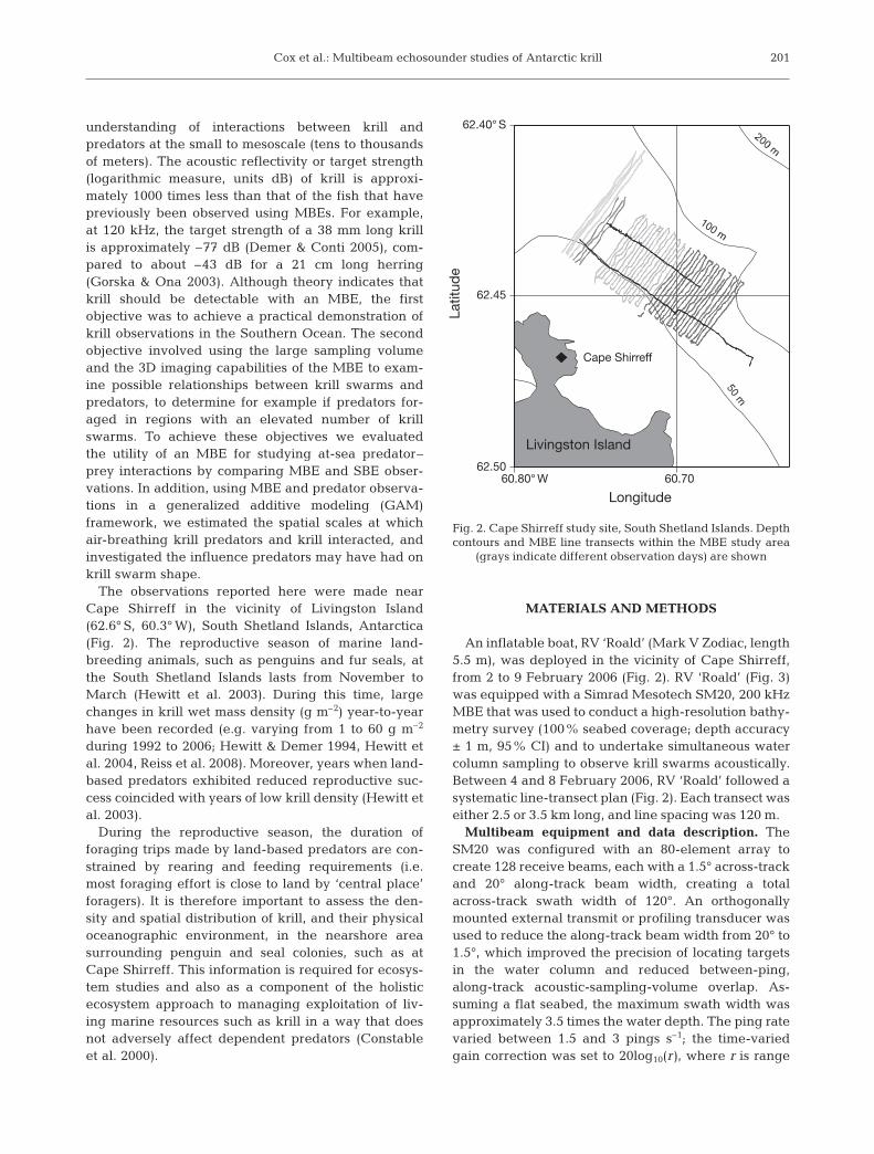
The MBE was housed in a blister fairing (Fig. 3)mounted on a retractable frame which, when de-ployed, positioned the SM20 transducers along thecenter line of RV ‘Roald’, with the center beam of theMBE positioned vertically downward, giving a 60°swath to both sides of the boat and perpendicular tothe transect. This MBE orientation permitted simulta-neous observations of the bathymetry and water col-umn targets. The MBE observations were logged con-tinuously to the SM20 control computer. Water columndata (Sv in dB, for each 0.5 m sample) were convertedto the SM2000 data format using a Simrad utility(MsToSm v1.0) and processed using Echoview v3.50(SonarData). Krill swarms were identified using the‘cruise scanning 3D schools detection algorithm’ de-veloped by SonarData (see Cox et al. 2009 for sensitiv-ity analysis of 3D detection parameters), and krillswarm metrics were extracted. Optimized swarm de-tection parameters were (1) processing threshold =24 dB (uncalibrated); and (2) minimum longest, middleand shortest dimensions = 5 m (Cox 2008, Cox et al.2009).

The MBE operated at one frequency, so it was notpossible to use multifrequency techniques (e.g. Brier-ley et al. 1998) to partition echoes by species. However,based on an analysis of multifrequency data obtainedwith a conventional scientific echosounder in the same

area from a second inflatable boat (RV ‘Ernest’, left-hand vessel in Fig. 3), all MBE-detected aggregationswere assumed to be krill swarms. The calibrated, dual-frequency (38 and 200 kHz) echosounder data (SimradES60) were collected by RV ‘Ernest’ within 5 km of thecenter of the multibeam study site (Fig. 2) and wereanalyzed following the methods of Brierley et al.(1998). That analysis indicated that 96.3% of thepelagic aggregations by number were indeed Antarc-tic krill swarms.

We sought to examine variability in krill swarm char-acteristics throughout the survey area. Simple linearmeasures of swarm dimensions may not accuratelyrepresent a swarm with a potentially complex shape.Linear measurements of water column aggregationsare often based on a 3D bounding box placed aroundthe aggregation. Such boxes only define an aggrega-tion’s maximum x, y and z dimensions (Gerlotto &Paramo 2003). As an advance on this, the 3D shape ofa krill swarm was further quantified here using theroughness (R), calculated as the swarm surface area(A) divided by its volume (V). Following the proceduregiven in Gerlotto & Paramo (2003), R values for acousti-cally detected swarms were compared to those of 3standard geometric shapes: a sphere; a cylinder, andan ellipsoid. To calculate the R for these standard geo-metric shapes, the observed swarm V values wereused, and the A values were calculated in the appro-priate manner from V for each shape: for spheres, Avalues were calculated directly from the observed V;

for cylinders, A values were calculatedfrom the observed V and swarm heights(H), and for ellipsoids, the lengths of theaxes lengths and thus A values werecalculated from the dimensions ofthe 3D bounding box, measured usingEchoview v3.5.

Predator–prey interactions. To assessthe spatial overlap between air-breath-ing predators and krill, visual observa-tions of predators were made from RV‘Roald’ and RV ‘Ernest’, by a trained ob-server, concurrent with the multibeamsampling. Predators were detected for-ward of the protective dodger (1 m backfrom the boat’s bow, see Fig. 3) to arange of ca. 50 m. Predator type, eitherswimming or flying, group size, activity(e.g. foraging, traveling), location andtime of observation were recorded forthe following predator species: Antarc-tic tern Sterna vittata; black-browedalbatross Thalassarche melanophris;black-bellied storm petrel Fregetta tro-pica; chinstrap penguin Pygoscelis ant-

202

Fig. 3. The MBE-equipped RV ‘Roald’ (right-hand vessel) and single-beamechosounder (SBE)-equipped RV ‘Ernest’. The MBE blister fairing (white) wasmounted on a rotating frame attached to the Zodiac’s transom (it is visible in the

‘up’ position through the transparent side of the dodger)

Cox et al.: Multibeam echosounder studies of Antarctic krill

arctica; Antarctic fur seal Arctocephalus sp. (gazella);gray-headed albatross Thalassarche chrysostoma;humpback whale Megaptera novaeangliae; south polarskua Catharacta maccormicki; giant petrel (unidenti-fied) Macronectes sp.; penguin (unidentified) Pygos-celis/Eudyptes sp.; and Wilson’s storm petrel Oceanitesoceanicus. Bearing angles to predators were estimatedusing a compass, and ranges were estimated usingmarks on the dodger. Rapid and frequent changes inthe boat heading due to waves probably introduced er-rors in some of the measurements of off-transect dis-tances to predators.

The interactions between krill swarms and predatorswere investigated using predator sighting data observedfrom RV ‘Roald’ (see Table 2). Since there was no a priorireason to expect a linear response between swarmroughness and potential explanatory variables suchas swarm or predator nearest-neighbor distance (NND)or seabed depth, GAMs were used to investigate thecauses of variability in krill swarm roughness (analysisin R v2.4.0, mgcv library v1.3-19; R Development CoreTeam 2007). GAMs can be thought of as conventionalregressions with the coefficients replaced by smoothfunctions, in this instance thin-plate regression splines,and are useful when relationships between explanatoryand response variables are non-linear (Venables & Dich-mont 2004, Wood 2006). In the present study, a variety ofcombinations of explanatory variables were used, andthe best GAM from a variety of candidate GAMs wasselected in the conventional way on the basis of Akaikeinformation criteria (AIC; Akaike 1974).

Variability in the number of krill swarms detected inthe vicinity of a predator encountered by both boatswas determined using an annulus sampler (Fig. 4). Foreach predator encounter, the number of krill swarms

within a given area surrounding the position of a pre-dator was calculated by laying down first a samplingcircle of radius = 50 m, followed by a series of concen-tric annuli with constant areas of 7854 m2 (equivalentto the area of a circle of radius = 50 m, Fig. 4A). Con-secutive sampling annuli were laid down at increasingranges (Fig. 4B,C). Annuli more distant from the centerhad narrower inner to outer separations. The maxi-mum total radius of this sampling was 274 m and com-prised 30 sampling annuli. A GAM was fitted to themean number of krill swarms detected in each annu-lus, at each sampling location. For each boat the totalnumber of swarms in each sampling annulus was cal-culated for all predator encounters.

A simulation procedure was devised to examine po-tential differences between the number of krill swarmsin the vicinity of predators and krill swarms in areaswithout predators. For each simulation, the annulussampler, described above, was centered on x randomlyselected transect positions, where x = 41 = the numberof predator groups encountered. The simulation proce-dure was repeated 1000 times, and for each simulationa GAM was fitted to the mean number of krill swarmsin each of the annulus sampling areas. The mean simu-lated GAM curves and associated standard errors weredetermined, and differences between the simulatedand observed mean numbers of swarms were assessedusing a 2-sample Kolmogorov-Smirnov test.

RESULTS

A total of 1084 krill swarms were detected by theMBE. Seabed depth in the survey area ranged from 20to 140 m; this is important to consider, as seabed depth

203

50 m 20.7 m 15.9 m

A B Cn1 = 4 n2 = 7 n3 = 4

Fig. 4. Plan view of the annulus sampler (constant area = 7854 m2) defined around predator positions. (A) Circular sampling area(n1, radius = 50 m) centered on an example predator location in which 4 predators were seen and, sequentially, the (B) first and2nd concentric donuts (n2 and n3) in which 7 and 4 predators were seen respectively. In this example, the sampling area is shown

in gray, with krill swarms in the area (x) and outside (o)

Mar Ecol Prog Ser 378: 199–209, 2009

determines the MBE sampling volume and maximumobservable across-track swarm width (70 m at 20 mwater depth and 485 m at 140 m water depth). MBEsampling volume is further reduced by side lobe detec-tions of the seabed (Fig. 1), as krill swarms cannot bedetected within the side lobe interference. Of the 1084detected krill swarms, 78 were found to be truncatedby side-lobe interference; thus 1006 krill swarms weredetermined to be entirely within the MBE effectivesampling volume (Fig. 1) and used in subsequentanalyses (Table 1).

During the survey, 41 foraging predator groups wereencountered during the RV ‘Roald’ MBE survey, com-

prising a total of 54 individual preda-tors (Table 2), of both swimming(18 ind.) and flying (36 ind.) types.During the RV ‘Ernest’ SBE survey,both swimming (17 ind.) and flying(41 ind.) predators were encounteredwithin 5 km of the MBE study site. Thepredator type (swimming or flying)was used as a factor variable in theGAM investigating the variation inswarm roughness (Table 3).

Swarm roughness

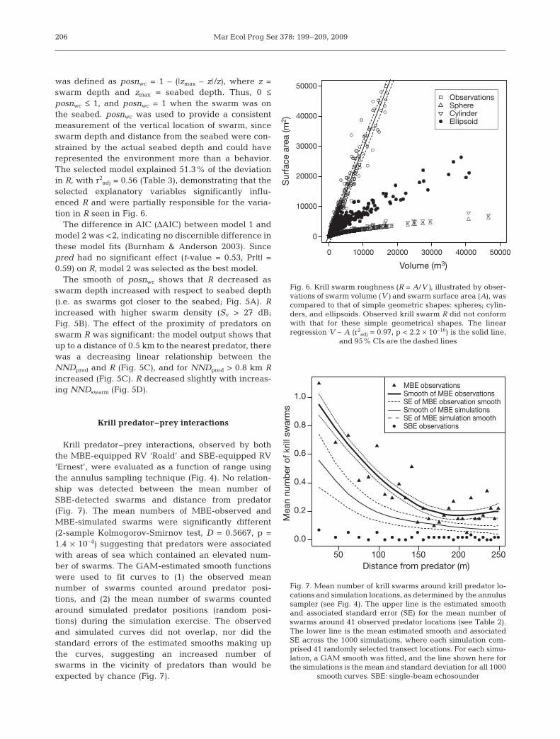
The observed R of krill swarmsranged from 1.2 to 8.1 (mean R = 3.3;Table 1), and did not conform with theR values expected for any of the sim-ple geometric shapes considered:spheres have the lowest mean R of0.53, followed by cylinders (mean R =0.68), and then ellipsoids (mean R =2.0, Fig. 6). This suggests that krillswarm geometries cannot reliably beapproximated by these simple shapes.

204

Metric Mean (CV) Range

A (m2) 11 024.7 (4.70) 218.6–1 222 048V (m3) 3695.7 (4.59) 46.2–406 709.8R (m–1) 3.3 (0.23) 1.2–8.1Sv mean (dB re 1 m2/m3) 22.7 (0.14) 13.6–45.0posnwc 0.6 (0.32) 0–1.0

Table 1. Summary statistics for the 1006 swarms that werelocated entirely within the multibeam echosounder swath.A: surface area; V: volume; R: roughness; Sv: uncalibratedacoustic mean volume backscattering strength; posnwc:position in the water column; CV: coefficient of variation

Predator Number of individuals PredatorRV ‘Roald’ RV ‘Ernest’ type

Sterna vittata 10 7 FlyingAntarctic tern

Thalassarche melanophris 8 9 Flyingblack-browed albatross

Fregetta tropica 3 0 Flyingblack-bellied storm petrel

Pygoscelis antarctica 1 6 Swimmingchinstrap penguin

Arctocephalus sp. (gazella) 6 1 SwimmingAntarctic fur seal

Thalassarche chrysostoma 0 4 Flyinggray-headed albatross

Megaptera novaeangliae 4 7 Swimminghumpback whale

Catharacta maccormicki 2 0 Flyingsouth polar skua

Macronectes sp. 1 9 Flyinggiant petrel (unid.)

Pygoscelis/Eudyptes sp. 7 3 Swimmingpenguin (unid.)

Oceanites oceanicus 12 12 FlyingWilson’s storm petrel

Table 2. Foraging predators observed from RV ‘Roald’ in the multibeam studysite and from RV ‘Ernest’ within 5 km of the center of the multibeam study site.

unid.: unidentified

Model number Explanatory variables r2adj Deviance explained (%) AIC ΔAIC

1 NNDpred + NNDswarm + posnwc + Sv + pred 0.56 51.3 1598.1 +1.7

2 NNDpred + NNDswarm + posnwc + Sv 0.56 51.3 1596.4 0

3 NNDpred + NNDswarm + posnwc 0.55 49.0 1634.0 +37.6

4 NNDpred + NNDswarm 0.15 14.4 2092.8 +496.4

5 NNDpred 0.11 11.4 2121.2 524.8

Table 3. Example candidate generalized additive models (GAMs) explaining swarm roughness. Explanatory variables consid-ered in this example subset of candidate GAMs were swarm position in water column (posnwc), mean swarm volume backscatter-ing strength (Sv), nearest-neighbor distance between swarms (NNDswarm) and distance to nearest predator (NNDpred). Modelswere selected using Akaike information criteria (AIC). Model 1 was selected since the difference in AIC (ΔAIC) between thismodel and model 2 was <2 (Burnham & Anderson 2003), and this enabled examination of the potential influence of predator type

(swimming or flying, pred) on R

Cox et al.: Multibeam echosounder studies of Antarctic krill

The low variance of R is illustrated by the confidenceintervals (CIs) of the linear regression (V ~ A, r2

adj =0.97, p < 2.2 × 10–16; Fig. 6). The low variance of the ob-served R, compared to those for A and V, suggests thatkrill behave collectively to maintain a preferred swarmR (Table. 1).

Factors affecting swarm roughness

All candidate GAMs describing the variation in krillswarm R had a log-link function and a gamma-errordistribution, which were selected so the model resultswould not violate model assumptions (Wood 2006).Various combinations of krill swarm descriptors

(Table 1) were considered as potential explanatoryvariables to explain variation in R in the GAM (seeTable 3 for an example subset of possible explanatoryvariable combinations), and the best GAM model wasselected from candidate GAM models on the basis oflowest AIC (Table 3).

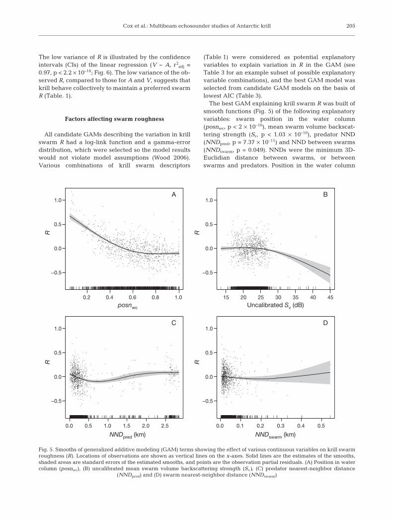
The best GAM explaining krill swarm R was built ofsmooth functions (Fig. 5) of the following explanatoryvariables: swarm position in the water column(posnwc, p < 2 × 10–16), mean swarm volume backscat-tering strength (Sv, p < 1.03 × 10–10), predator NND(NNDpred, p = 7.37 × 10–11) and NND between swarms(NNDswarm, p = 0.049). NNDs were the minimum 3D-Euclidian distance between swarms, or betweenswarms and predators. Position in the water column

205

0.2 0.4 0.6 0.8 1.0

−0.5

0.0

0.5

1.0

posnwc

A

15 20 25 30 35 40 45

−0.5

0.0

0.5

1.0

Uncalibrated Sv (dB)

B

0.0 0.5 1.0 1.5 2.0 2.5

−0.5

0.0

0.5

1.0C

0.0 0.1 0.2 0.3 0.4 0.5

−0.5

0.0

0.5

1.0D

NNDswarm (km)NNDpred (km)

R R

R R

Fig. 5. Smooths of generalized additive modeling (GAM) terms showing the effect of various continuous variables on krill swarmroughness (R). Locations of observations are shown as vertical lines on the x-axes. Solid lines are the estimates of the smooths,shaded areas are standard errors of the estimated smooths, and points are the observation partial residuals. (A) Position in watercolumn (posnwc), (B) uncalibrated mean swarm volume backscattering strength (Sv), (C) predator nearest-neighbor distance

(NNDpred) and (D) swarm nearest-neighbor distance (NNDswarm)

Mar Ecol Prog Ser 378: 199–209, 2009

was defined as posnwc = 1 – (|zmax – z|/z), where z =swarm depth and zmax = seabed depth. Thus, 0 ≤posnwc ≤ 1, and posnwc = 1 when the swarm was onthe seabed. posnwc was used to provide a consistentmeasurement of the vertical location of swarm, sinceswarm depth and distance from the seabed were con-strained by the actual seabed depth and could haverepresented the environment more than a behavior.The selected model explained 51.3% of the deviationin R, with r2

adj = 0.56 (Table 3), demonstrating that theselected explanatory variables significantly influ-enced R and were partially responsible for the varia-tion in R seen in Fig. 6.

The difference in AIC (ΔAIC) between model 1 andmodel 2 was <2, indicating no discernible difference inthese model fits (Burnham & Anderson 2003). Sincepred had no significant effect (t-value = 0.53, Pr|t| =0.59) on R, model 2 was selected as the best model.

The smooth of posnwc shows that R decreased asswarm depth increased with respect to seabed depth(i.e. as swarms got closer to the seabed; Fig. 5A). Rincreased with higher swarm density (Sv > 27 dB;Fig. 5B). The effect of the proximity of predators onswarm R was significant: the model output shows thatup to a distance of 0.5 km to the nearest predator, therewas a decreasing linear relationship between theNNDpred and R (Fig. 5C), and for NNDpred > 0.8 km Rincreased (Fig. 5C). R decreased slightly with increas-ing NNDswarm (Fig. 5D).

Krill predator–prey interactions

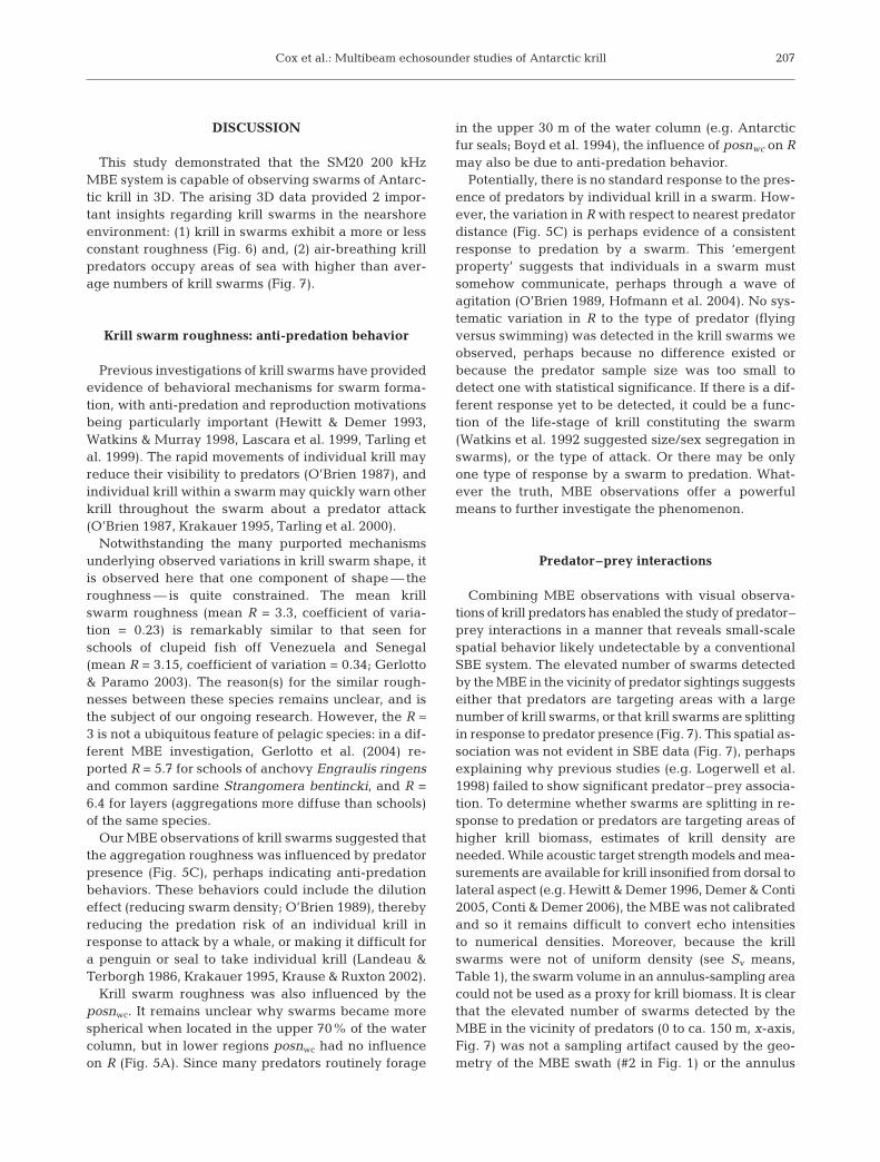
Krill predator–prey interactions, observed by boththe MBE-equipped RV ‘Roald’ and SBE-equipped RV‘Ernest’, were evaluated as a function of range usingthe annulus sampling technique (Fig. 4). No relation-ship was detected between the mean number ofSBE-detected swarms and distance from predator(Fig. 7). The mean numbers of MBE-observed andMBE-simulated swarms were significantly different(2-sample Kolmogorov-Smirnov test, D = 0.5667, p =1.4 × 10–4) suggesting that predators were associatedwith areas of sea which contained an elevated num-ber of swarms. The GAM-estimated smooth functionswere used to fit curves to (1) the observed meannumber of swarms counted around predator posi-tions, and (2) the mean number of swarms countedaround simulated predator positions (random posi-tions) during the simulation exercise. The observedand simulated curves did not overlap, nor did thestandard errors of the estimated smooths making upthe curves, suggesting an increased number ofswarms in the vicinity of predators than would beexpected by chance (Fig. 7).

206

0 10000 20000 30000 40000 50000

0

10000

20000

30000

40000

50000

Volume (m3)

Surf

ace a

rea (m

2)

ObservationsSphereCylinderEllipsoid

Fig. 6. Krill swarm roughness (R = A/V), illustrated by obser-vations of swarm volume (V) and swarm surface area (A), wascompared to that of simple geometric shapes: spheres; cylin-ders, and ellipsoids. Observed krill swarm R did not conformwith that for these simple geometrical shapes. The linearregression V ~ A (r2

adj = 0.97, p < 2.2 × 10–16) is the solid line, and 95% CIs are the dashed lines

50 100 150 200 250

0.0

0.2

0.4

0.6

0.8

1.0

Distance from predator (m)

Mean

nu

mb

er

of

krill

sw

arm

s

MBE observationsSmooth of MBE observationsSE of MBE observation smooth Smooth of MBE simulationsSE of MBE simulation smoothSBE observations

Fig. 7. Mean number of krill swarms around krill predator lo-cations and simulation locations, as determined by the annulussampler (see Fig. 4). The upper line is the estimated smoothand associated standard error (SE) for the mean number ofswarms around 41 observed predator locations (see Table 2).The lower line is the mean estimated smooth and associatedSE across the 1000 simulations, where each simulation com-prised 41 randomly selected transect locations. For each simu-lation, a GAM smooth was fitted, and the line shown here forthe simulations is the mean and standard deviation for all 1000

smooth curves. SBE: single-beam echosounder

Cox et al.: Multibeam echosounder studies of Antarctic krill

DISCUSSION

This study demonstrated that the SM20 200 kHzMBE system is capable of observing swarms of Antarc-tic krill in 3D. The arising 3D data provided 2 impor-tant insights regarding krill swarms in the nearshoreenvironment: (1) krill in swarms exhibit a more or lessconstant roughness (Fig. 6) and, (2) air-breathing krillpredators occupy areas of sea with higher than aver-age numbers of krill swarms (Fig. 7).

Krill swarm roughness: anti-predation behavior

Previous investigations of krill swarms have providedevidence of behavioral mechanisms for swarm forma-tion, with anti-predation and reproduction motivationsbeing particularly important (Hewitt & Demer 1993,Watkins & Murray 1998, Lascara et al. 1999, Tarling etal. 1999). The rapid movements of individual krill mayreduce their visibility to predators (O’Brien 1987), andindividual krill within a swarm may quickly warn otherkrill throughout the swarm about a predator attack(O’Brien 1987, Krakauer 1995, Tarling et al. 2000).

Notwithstanding the many purported mechanismsunderlying observed variations in krill swarm shape, itis observed here that one component of shape — theroughness — is quite constrained. The mean krillswarm roughness (mean R = 3.3, coefficient of varia-tion = 0.23) is remarkably similar to that seen forschools of clupeid fish off Venezuela and Senegal(mean R = 3.15, coefficient of variation = 0.34; Gerlotto& Paramo 2003). The reason(s) for the similar rough-nesses between these species remains unclear, and isthe subject of our ongoing research. However, the R ≈3 is not a ubiquitous feature of pelagic species: in a dif-ferent MBE investigation, Gerlotto et al. (2004) re-ported R = 5.7 for schools of anchovy Engraulis ringensand common sardine Strangomera bentincki, and R =6.4 for layers (aggregations more diffuse than schools)of the same species.

Our MBE observations of krill swarms suggested thatthe aggregation roughness was influenced by predatorpresence (Fig. 5C), perhaps indicating anti-predationbehaviors. These behaviors could include the dilutioneffect (reducing swarm density; O’Brien 1989), therebyreducing the predation risk of an individual krill inresponse to attack by a whale, or making it difficult fora penguin or seal to take individual krill (Landeau &Terborgh 1986, Krakauer 1995, Krause & Ruxton 2002).

Krill swarm roughness was also influenced by theposnwc. It remains unclear why swarms became morespherical when located in the upper 70% of the watercolumn, but in lower regions posnwc had no influenceon R (Fig. 5A). Since many predators routinely forage

in the upper 30 m of the water column (e.g. Antarcticfur seals; Boyd et al. 1994), the influence of posnwc on Rmay also be due to anti-predation behavior.

Potentially, there is no standard response to the pres-ence of predators by individual krill in a swarm. How-ever, the variation in R with respect to nearest predatordistance (Fig. 5C) is perhaps evidence of a consistentresponse to predation by a swarm. This ‘emergentproperty’ suggests that individuals in a swarm mustsomehow communicate, perhaps through a wave ofagitation (O’Brien 1989, Hofmann et al. 2004). No sys-tematic variation in R to the type of predator (flyingversus swimming) was detected in the krill swarms weobserved, perhaps because no difference existed orbecause the predator sample size was too small todetect one with statistical significance. If there is a dif-ferent response yet to be detected, it could be a func-tion of the life-stage of krill constituting the swarm(Watkins et al. 1992 suggested size/sex segregation inswarms), or the type of attack. Or there may be onlyone type of response by a swarm to predation. What-ever the truth, MBE observations offer a powerfulmeans to further investigate the phenomenon.

Predator–prey interactions

Combining MBE observations with visual observa-tions of krill predators has enabled the study of predator–prey interactions in a manner that reveals small-scalespatial behavior likely undetectable by a conventionalSBE system. The elevated number of swarms detectedby the MBE in the vicinity of predator sightings suggestseither that predators are targeting areas with a largenumber of krill swarms, or that krill swarms are splittingin response to predator presence (Fig. 7). This spatial as-sociation was not evident in SBE data (Fig. 7), perhapsexplaining why previous studies (e.g. Logerwell et al.1998) failed to show significant predator–prey associa-tion. To determine whether swarms are splitting in re-sponse to predation or predators are targeting areas ofhigher krill biomass, estimates of krill density areneeded. While acoustic target strength models and mea-surements are available for krill insonified from dorsal tolateral aspect (e.g. Hewitt & Demer 1996, Demer & Conti2005, Conti & Demer 2006), the MBE was not calibratedand so it remains difficult to convert echo intensitiesto numerical densities. Moreover, because the krillswarms were not of uniform density (see Sv means,Table 1), the swarm volume in an annulus-sampling areacould not be used as a proxy for krill biomass. It is clearthat the elevated number of swarms detected by theMBE in the vicinity of predators (0 to ca. 150 m, x-axis,Fig. 7) was not a sampling artifact caused by the geo-metry of the MBE swath (#2 in Fig. 1) or the annulus

207

Mar Ecol Prog Ser 378: 199–209, 2009

sampling regions (Fig. 4). If the curve of mean observednumber of swarms (Fig. 7) was driven by geometryalone, then the mean observed number of swarms andthe mean simulated number of swarms curves wouldhave overlapped.

Multibeam echosounder utility

An advantage of using an MBE over the SBE is thatthe volume and surface area of pelagic aggregationscan be observed directly, rather than derived from anassumed 3D shape. Simmonds & MacLennan (2005)presented a statistical technique that enabled themean area of an aggregation to be determined fromSBE observations by assuming that aggregations havea circular horizontal cross-section (i.e. assuming eitherspherical or cylindrical shapes). Here it is shown that inthe case of krill swarms, neither assumption is valid.While the ellipsoid had the closest roughness to theMBE-observed roughness (Fig. 6), the ellipsoid re-quires 3 length measurements to approximate areaand volume, whereas only swarm length and heightare available from SBE observations. This finding indi-cates that extrapolation of SBE observations to 3D can-not be used to estimate swarm shape or roughness.

CONCLUSIONS

This investigation has demonstrated that krillswarms can be detected and described in 3D with a200 kHz MBE, and that the external envelope of krillswarms cannot be accurately described by simple geo-metric shapes. It appears that krill swarms maintain asimilar roughness irrespective of shape, perhaps as aresponse to predator presence. The increased sam-pling volume of the MBE compared to the SBE used inthis investigation revealed a previously undetectedelevated number of krill swarms in the vicinity of air-breathing predators.

Acknowledgements. We thank the Royal Society for fundsenabling deployment of the MBE; Simrad USA, particularlyJeff Condiotty, for the loan of the SM20, and D. Needham andM. Patterson of Sea Technology Services for designing andconstructing the transducer mount. We are grateful to theUnited States Antarctic Marine Living Resources Program;the Master, officers and crew of the RV ‘Yuzhmorgeologiya’,and the personnel at the Cape Shirreff field station for logisti-cal, equipment and ship support. M.J.C. was supported by aNERC PhD studentship. This work was carried out in associa-tion with an NSF-funded (grant #06-OPP-33939) investigationof the Livingston Island nearshore environment. We thank A.Jenkins, T. S. Sessions and M. van den Berg for skipperingthe nearshore boats, and T. S. Sessions for providing invalu-able expertise in the field.

LITERATURE CITED

Akaike H (1974) A new look at the statistical model identifica-tion. IEEE Trans Automat Contr 19:716–723

Atkinson A, Whitehouse MJ, Priddle J, Cripps GC, Ward P,Brandon MA (2001) South Georgia, Antarctica: a produc-tive, cold water, pelagic ecosystem. Mar Ecol Prog Ser 216:279–308

Axelsen BE, Anker-Nilssen T, Fossum P, Kvamme C, NøttestadL (2001) Pretty patterns but a simple strategy: predator–prey interactions between juvenile herring and Atlanticpuffins observed with multibeam sonar. Can J Zool 79:1586–1596

Boyd IL, Arnould JPY, Barton T, Croxall JP (1994) Foragingbehaviour of Antarctic fur seals during periods of contrast-ing prey abundance. J Anim Ecol 63:703–713

Brierley AS, Ward P, Watkins JL, Goss C (1998) Acoustic dis-crimination of Southern Ocean zooplankton. Deep-SeaRes II 45:1155–1173

Brierley AS, Watkins JL, Goss C, Wilkinson MT, Everson I(1999) Acoustic estimates of krill density at South Georgia,1981 to 1998. CCAMLR Sci 6:47–57

Burnham KP, Anderson DR (2003) Model selection andmultimodel inference: a practical information-theoreticapproach, 2nd edn Springer, New York

Constable AJ, de la Mare WK, Agnew DJ, Everson I, Miller D(2000) Managing fisheries to conserve the Antarcticmarine ecosystem: practical implementation of the Con-vention on the Conservation of Antarctic Marine LivingResources (CCAMLR). ICES J Mar Sci 57:778–791

Conti SG, Demer DA (2006) Improved parameterization of theSDWBA for estimating krill target strength. ICES J MarSci 63:928–935

Cox MJ (2008) Acoustic and ecological investigations intopredator–prey interactions between Antarctic krill(Euphausia superba) and seal and bird predators. PhDthesis, University of St. Andrews, Fife

Cox MJ, Warren JD, Demer DA, Cutter GR, Brierley AS(2009) Three-dimensional observations of Antarctic krill(Euphausia superba) swarms made using a multi-beamechosounder. Deep-Sea Res II (in press)

Demer DA, Conti SG (2005) New target-strength model indi-cates more krill in the Southern Ocean. ICES J Mar Sci 62:25–32

Gerlotto F, Paramo J (2003) The three-dimensional morpho-logy and internal structure of clupeid schools as observedusing vertical scanning multibeam sonar. Aquat LivingResour 16:113–122

Gerlotto F, Soria M, Freon P (1999) From two dimensions tothree: the use of multibeam sonar for a new approach infisheries acoustics. Can J Fish Aquat Sci 56:6–12

Gerlotto F, Castillo J, Saavedra A, Barbieri MA, Espejo M,Cotel P (2004) Three-dimensional structure and avoidancebehaviour or anchovy and common sardine schools incentral Chile. ICES J Mar Sci 61:1120–1126

Gorska N, Ona E (2003) Modelling the acoustic effect of swim-bladder compression in herring. ICES J Mar Sci 60:548–554

Hewitt RP, Demer DA (1993) Dispersion and abundance ofAntarctic krill in the vicinity of Elephant Island in the 1992austral summer. Mar Ecol Prog Ser 99:29–39

Hewitt RP, Demer DA (1994) Acoustic estimates of krill biomassin the Elephant Island area: 1981–1993. CCAMLR Sci 1:1–5

Hewitt RP, Demer DA (1996) Lateral target strength ofAntarctic krill. ICES J Mar Sci 53:297–302

Hewitt RP, Demer DA (2000) The use of acoustic sampling toestimate the dispersion and abundance of euphausiids,

208

Cox et al.: Multibeam echosounder studies of Antarctic krill

with an emphasis on Antarctic krill, Euphausia superba.Fish Res 47:215–229

Hewitt RP, Demer DA, Emery JH (2003) An 8-year cycle inkrill biomass density inferred from acoustic surveys con-ducted in the vicinity of the South Shetland Islands duringthe austral summers of 1991-1992 through 2001-2002.Aquat Living Resour 16:205–213

Hewitt RP, Watkins J, Naganobu M, Sushin V and others(2004) Biomass of Antarctic krill in the Scotia sea in Janu-ary/February 2000 and its use in revising an estimate ofprecautionary yield. Deep-Sea Res II 51:1215–1236

Hofmann EE, Haskell AGE, Klinck JM, Lascara CM (2004)Lagrangian modelling studies of Antarctic krill (Euphau-sia superba) swarm formation. ICES J Mar Sci 61:617–631

Krakauer DC (1995) Groups confuse predators by exploitingperceptual bottlenecks: a connectionist model of theconfusion effect. Behav Ecol Sociobiol 36:421–429

Krause J, Ruxton GD (2002) Living in groups. Oxford Univer-sity Press, Oxford

Landeau L, Terborgh J (1986) Oddity and the confusion effectin predation. Anim Behav 34:1372–1380

Lascara CM, Hofmann EE, Ross RM, Quetin LB (1999) Sea-sonal variability in the distribution of Antarctic krill,Euphausia superba, west of the Antarctic Peninsula.Deep-Sea Res I 46:951–984

Logerwell EA, Hewitt RP, Demer DA (1998) Scale-dependentspatial variance patterns and correlations of seabirds andprey in the southeastern Bering Sea as revealed by spec-tral analysis. Ecography 21:212–223

Mangel M, Nicol S (2000) Krill and the unity of biology. Can JFish Aquat Sci 57:1–5

O’Brien DP (1987) Description of escape responses of krill(Crustacea: Eupausiacea), with particular reference toswarming behavior and the size and proximity of thepredator. J Crustac Biol 7:449–457

O’Brien DP (1989) Analysis of the internal arrangement ofindividuals within crustacean aggregations (Eupausiacea,Mysidacea). J Exp Mar Biol Ecol 128:1–30

Paramo J, Bertrand S, Villalobos H, Gerlotto F (2007) A three-

dimensional approach to school typology using verticalscanning multibeam sonar. Fish Res 84:171–179

R Development Core Team (2007). R: a language andenvironment for statistical computing. R Foundation forStatistical Computing, Vienna

Reid DG, Simmonds EJ (1993) Image analysis techniques forthe study of fish school structure from acoustic surveydata. Can J Fish Aquat Sci 50:886–893

Reiss CS, Cossio AM, Loeb V, Demer DA (2008) Variations inthe biomass of Antarctic krill (Euphausia superba) aroundthe South Shetland Islands, 1996–2006. ICES J Mar Sci 65:497–508

Simmonds JE, MacLennan DN (2005) Fisheries acoustics:theory and practice, 2nd edn Chapman & Hall, London

Tarling GA, Cuzin-Roudy J, Buchholz F (1999) Verticalmigration behaviour in the northern krill Meganycti-phanes norvegica is influenced by moult and reproductiveprocesses. Mar Ecol Prog Ser 190:253–262

Tarling G, Burrows M, Matthews J, Saborowski R, BuchholzF, Bedo A, Mayzaud P (2000) An optimisation model of thediel vertical migration of northern krill (Meganyctiphanesnorvegica) in the Clyde Sea and the Kattegat. Can J FishAquat Sci 57(S3):38–50

Venables WN, Dichmont CM (2004) GLMs, GAMs andGLMMs: an overview of theory for applications in fish-eries research. Fish Res 70:319–337

Watkins JL, Murray AWA (1998) Layers of Antarctic krill,Euphausia superba: are they just long krill swarms? MarBiol 131:237–247

Watkins JL, Buchholz F, Priddle J, Morris DJ, Ricketts C(1992) Variation in reproductive status of Antarctic krillswarms; evidence of size-related sorting mechanism? MarEcol Prog Ser 82:163–174

Wood SN (2006) Generalized additive models: an introductionwith R. Chapman & Hall, London

Zamon JE, Greene CH, Meir E, Demer DA, Hewitt RP, SextonS (1996) Acoustic characterization of the three-dimen-sional prey field of foraging chinstrap penguins. Mar EcolProg Ser 131:1–10

209

Editorial responsibility: Rory Wilson,Swansea, UK

Submitted: October 8, 2007; Accepted: October 23, 2008Proofs received from author(s): March 11, 2009