Multi-Physics Simulation of Friction stir welding process ·  · 2013-10-17Multi-Physics Simulation of Friction stir welding process Hongjun Li, Donald Mackenzie and Robert Hamilton*

Multi-Physics Simulation of Friction stir welding process

Hongjun Li, Donald Mackenzie and Robert Hamilton*

Department of Mechanical Engineering University of Strathclyde

James Weir Building 75 Montrose Street

Glasgow, UK, G1 1XJ

Abstract

Purpose: The Friction Stir Welding (FSW) process comprises of several highly coupled (and

non-linear) physical phenomena: large plastic deformation, material flow transportation,

mechanical stirring of the tool, tool-workpiece surface interaction, dynamic structural evolution,

heat generation from friction and plastic deformation, etc. In this paper, an advanced Finite

Element (FE) model encapsulating this complex behavior is presented and various aspects

associated with the FE model such as contact modeling, material model and meshing techniques

are discussed in detail.

Methodology: The numerical model is continuum solid mechanics-based, fully thermo-

mechanically coupled and has successfully simulated the friction stir welding process including

plunging, dwelling and welding stages.

Findings: The development of several field variables are quantified by the model: temperature,

stress, strain, etc. Material movement is visualized by defining tracer particles at the locations of

interest. The numerically computed material flow patterns are in very good agreement with the

general findings from experiments.

Value: The model is, to the best of the authors’ knowledge, the most advanced simulation of

FSW published in the literature.

Keywords: Friction Stir Welding (FSW); Multi-physics; Numerical simulation

* Corresponding author, Tel.: +44 (0) 141 548 2046; Fax: +44 (0) 141 552 5105; Email: r.hamilton@strath.ac.uk

For Peer Review

Multi-Physics Simulation of Friction stir welding process

Journal: Engineering Computations

Manuscript ID: EC-Apr-2009-0027.R1

Manuscript Type: Research Article

Keywords: Friction Stir Welding (FSW), Multi-physics, Numerical simulation

http://mc.manuscriptcentral.com/engcom

Engineering Computations

For Peer Review

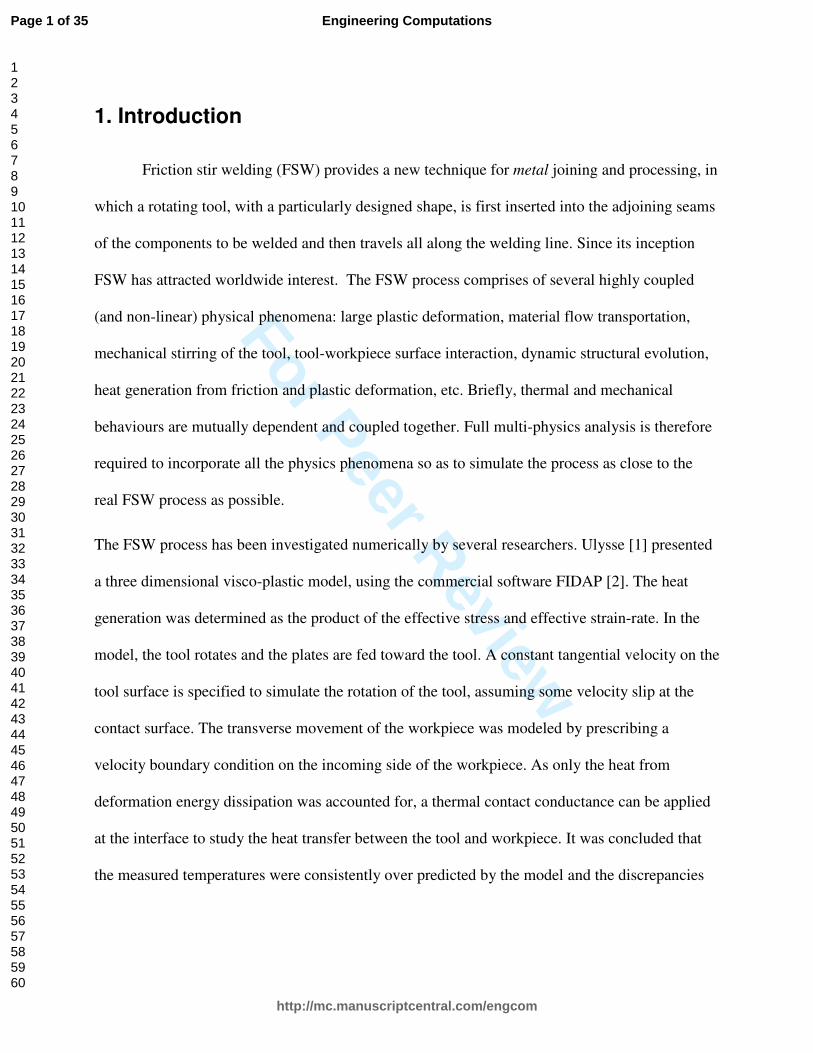
1. Introduction

Friction stir welding (FSW) provides a new technique for metal joining and processing, in

which a rotating tool, with a particularly designed shape, is first inserted into the adjoining seams

of the components to be welded and then travels all along the welding line. Since its inception

FSW has attracted worldwide interest. The FSW process comprises of several highly coupled

(and non-linear) physical phenomena: large plastic deformation, material flow transportation,

mechanical stirring of the tool, tool-workpiece surface interaction, dynamic structural evolution,

heat generation from friction and plastic deformation, etc. Briefly, thermal and mechanical

behaviours are mutually dependent and coupled together. Full multi-physics analysis is therefore

required to incorporate all the physics phenomena so as to simulate the process as close to the

real FSW process as possible.

The FSW process has been investigated numerically by several researchers. Ulysse [1] presented

a three dimensional visco-plastic model, using the commercial software FIDAP [2]. The heat

generation was determined as the product of the effective stress and effective strain-rate. In the

model, the tool rotates and the plates are fed toward the tool. A constant tangential velocity on the

tool surface is specified to simulate the rotation of the tool, assuming some velocity slip at the

contact surface. The transverse movement of the workpiece was modeled by prescribing a

velocity boundary condition on the incoming side of the workpiece. As only the heat from

deformation energy dissipation was accounted for, a thermal contact conductance can be applied

at the interface to study the heat transfer between the tool and workpiece. It was concluded that

the measured temperatures were consistently over predicted by the model and the discrepancies

Page 1 of 35

http://mc.manuscriptcentral.com/engcom

Engineering Computations

123456789101112131415161718192021222324252627282930313233343536373839404142434445464748495051525354555657585960

For Peer Review

probably resulted from an inadequate representation of the constitutive behaviour of the material

used in FSW.

Santiago et al [3] presented a similar model to [1] with the same rigid and visco-plastic

material model and the same modelling technique, in which the plates move towards the rotating

tool and the material flow at the interface is specified as a boundary condition. This model was

meshed with tetrahedral elements of the Taylor-Hood type, with quadratic interpolations for

velocities and linear interpolations for stresses. Because a static analysis method was used for

both models in [1] and [3], the results estimated from the models correspond to the steady state of

the FSW process. Schmidt and Hattel [4] put forward a fully coupled thermo-mechanical

dynamic analysis model also aiming to achieve the steady welding state using the arbitrary

Lagrangian-Eulerian formulation in ABAQUS/Explicit [5]. The solid elastic-plastic Johnson-

Cook material model was used:

( )[ ]

−

−−

++=

m

refmelt

refpl

npl

yTT

TTCBA 1ln1

0εε

εσ&

& (1)

where A, B, C, m, n, Tmelt and Tref are material constants, plε the effective plastic strain, plε& the

effective plastic strain rate and 0ε& the normalizing strain rate. A disc-shaped plate was created for

convenience of meshing. Similar to models in [1] and [3], a velocity equal to the welding speed

was assigned to the materials on the incoming side of the plate. At the tool-workpiece interface,

Coulomb’s Law of friction was used to model the contact behavior with a constant friction

coefficient of 0.3. The greatest improvement over the previous models was the ability to predict

the suitable thermo-mechanical conditions under which the weld can form.

Page 2 of 35

http://mc.manuscriptcentral.com/engcom

Engineering Computations

123456789101112131415161718192021222324252627282930313233343536373839404142434445464748495051525354555657585960

For Peer Review

Lasley [5] developed a fully coupled thermo-mechanical finite element model with the transient

explicit analysis capability to predict temperature evolution and material flow during the plunge

phase. The commercial software Forge3 [6] was used in the analysis, specializing in modeling of

high deformation forming processes which was handled by an automatic Lagrangian remeshing

scheme. The temperature and strain rate dependent viscoplastic Norton-Hoff model with the

Hansel and Spittel flow criteria was used in the model.

The most recent FSW model was proposed by Buffa et al [7] using DEFORM-3DTM[8], a

Lagrangian implicit code. The FSW process was modelled from the initial plunge state to steady

state travel. A non-uniform mesh with adaptive remeshing was adopted. A rigid-viscoplastic

material model was employed and material constants were determined by numerical regression

based on experimental data. It was assumed that the heat generation was due only to plastic and

frictional conditions at the tool-workpiece interface. The model was able to predict the

temperature, strain, strain rate as well as material flow and forces. Good agreement was obtained

when comparing the results of the simulation with experimental data.

For all the coupled models listed above, only those of Lasley [9] and Buffa et al [7]

attempted to simulate the full FSW process. Furthermore, the model in Lasley [9] can only

simulate the plunge stage. Their models gave good prediction of strain rate and material flow;

however, the deformation history information could not be obtained because a fluid-like

viscoplastic material model was used. The same problems occur in other Computational Fluid

Dynamic (CFD) models [10-18]. Schmidt and Hattel [4] used a material model with an elastic

contribution but only steady state was simulated. The objective of present paper is to extend FSW

numerical FE simulation to fully thermo-mechanically model the process using material models

that can return both temperature and (residual) stress results.

Page 3 of 35

http://mc.manuscriptcentral.com/engcom

Engineering Computations

123456789101112131415161718192021222324252627282930313233343536373839404142434445464748495051525354555657585960

For Peer Review

2. Numerical Model

2.1 Simulation method

The choice of finite element method appropriate to fully coupled simulation of the FSW

process is determined by a number of factors, including available models of physical phenomena,

meshing capabilities, solver technology and computing requirements.

The materials in contact with the rotating tool experience very large plastic deformations

and strains, and may move at a velocity close to that of the tool. In continuum solid mechanics

finite element analysis, there are two commonly used methods to tackle large strain/deformation

problems: Arbitrary Lagrangian-Eulerian (ALE) and complete remeshing formulations. ALE

combines the advantages of both Lagrangian and Eulerian methods and allows the mesh to move

independently of the material, making it possible to maintain a high-quality mesh during an

analysis. The mesh topology does not change in the model, which means that the number of

elements and their connectivity remains the same. In the FSW process, the tool travels a long

distance along the plate, the ALE approach may fail when mesh distortion reaches unacceptable

levels. To improve the simulation it would be necessary to use an FE technique which allowed

remeshing of the domain, however, the computational cost of such an approach is greater than

ALE and not all the FE codes incorporate a remeshing feature, (especially when using explicit

solvers).

Friction stir welding is a high-speed dynamic process that can be extremely costly to

analyze using implicit solvers. However, explicit solvers are well-suited for analyzing transient

dynamic response and in addition allow better representation of complex contact interactions

when the contact surface is not known a priori. The process itself is a coupled thermo-

mechanical process; hence an element with both temperature and displacement degrees of

Page 4 of 35

http://mc.manuscriptcentral.com/engcom

Engineering Computations

123456789101112131415161718192021222324252627282930313233343536373839404142434445464748495051525354555657585960

For Peer Review

freedom should be used. If the material is assumed to be viscoplatic, elements with mixed

formulation in terms of velocity and pressure fields are preferred. However, a viscoplastic model

cannot return residual stress as a result of the analysis. A temperature and strain rate dependent

material model incorporating the effect of elastic deformation is required to fully determine for

the flow, temperature, stress (residual) and strain of the workpiece material near the tool.

Taking the above factors into account, it was decided to base the simulation on

ABAQUS/EXPLICIT [5] analysis using the ALE formulation and a temperature and rate

dependent isotropic hardening plasticity material model to perform a fully coupled explicit

solution of the FSW process.

2.2 Governing equations and numerical formulations

2.2.1 Heater transfer equations

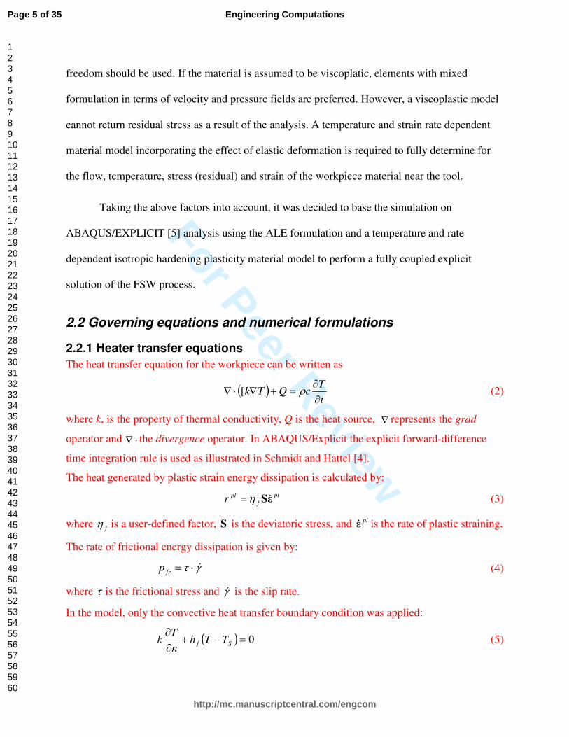
The heat transfer equation for the workpiece can be written as

( )t

TcQTk∂∂

=+∇⋅∇ ρ[ (2)

where k, is the property of thermal conductivity, Q is the heat source, ∇ represents the grad

operator and ∇ ⋅ the divergence operator. In ABAQUS/Explicit the explicit forward-difference

time integration rule is used as illustrated in Schmidt and Hattel [4].

The heat generated by plastic strain energy dissipation is calculated by:

pl

f

plr εS&η= (3)

where fη is a user-defined factor, S is the deviatoric stress, and plε& is the rate of plastic straining.

The rate of frictional energy dissipation is given by:

γτ &⋅=frp (4)

where τ is the frictional stress and γ& is the slip rate.

In the model, only the convective heat transfer boundary condition was applied:

( ) 0=−+∂∂

Sf TThn

Tk (5)

Page 5 of 35

http://mc.manuscriptcentral.com/engcom

Engineering Computations

123456789101112131415161718192021222324252627282930313233343536373839404142434445464748495051525354555657585960

For Peer Review

where fh is the film coefficient and ST the surrounding medium temperature.

2.2.2 Mechanical equations

The governing equation for the mechanical response of the process is the equilibrium equation:

( )σga div+= ρρ (6)

where σ is the stress tensor, g the body force per unit mass and a the acceleration.

In ABAQUS/Explicit the central difference rule is used as illustrated in Schmidt and Hattel [4].

2.2.3 Constitutive equations

The material model for the workpiece is chosen as temperature and rate dependent isotropic

hardening plasticity. The Johnson-Cook material law as expressed in Equation (1) was selected.

Hooke’s law is used to express the elasticity relationship,

( ) eleltrace εIεσ µλ 2+= (7)

where ( )1

ε ε ε

nel el el

ii iii

trace=

= = ∑ , λ and µ are elastic constants. Elastoplastic behaviour is

described by decomposing the strain rate or strain increment into elastic and plastic parts.

plel εεε &&& += (8)

Jaumann stress rate is employed to define the material behaviour, that is, the stress rate is purely

due to the elastic part of the strain rate and shown in terms of Hook’s law by

( ) eleltrace εIεσ &&& µλ 2+= (9)

or, in component fomat,

el

ij

el

kkijijσ εµελδ &&& 2+= (10)

the Jaumann rate equation is integrated in a corotational framework,

( ) eleltrace εIεσ ∆+∆=∆ µλ 2 (11)

The Mises yield function is assumed,

02

3=− yσS:S (12)

Page 6 of 35

http://mc.manuscriptcentral.com/engcom

Engineering Computations

123456789101112131415161718192021222324252627282930313233343536373839404142434445464748495051525354555657585960

For Peer Review

where ijij SS=S:S , yσ is uniaxial yield stress, is defined as a function of equivalent plastic

strain, strain rate and temperature. S is the deviatoric stress and p the hydrostatic pressure.

IσS p+= (13)

( )σtracep3

1−= (14)

Equivalent plastic strain is given by,

dt

t

plpl ∫=0

εε & (15)

plplplε:ε &&&

3

2=ε (16)

And the plastic flow law is:

pl

y

pl εσ

&&S

ε2

3= (17)

2.3 Model description

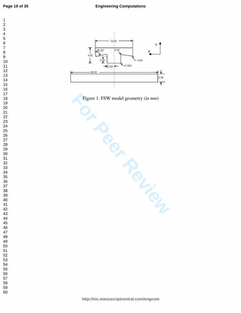
The FSW configuration modelled is shown in Figure 1. A single, complete plate was used

rather than two butted panels to give a continuum model. The workpiece is 60mm long, 30mm

wide and 3mm thick. The tool has a conical shoulder surface to accommodate material pushed

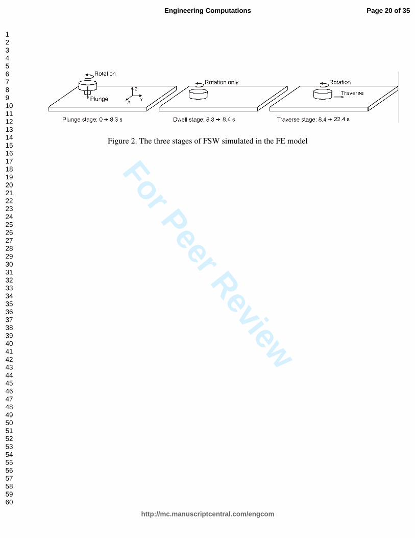
out when the tool probe is inserted into the plate. Three stages of the friction stir welding process

are modelled: plunge, dwell and traverse, as shown in Figure 2.

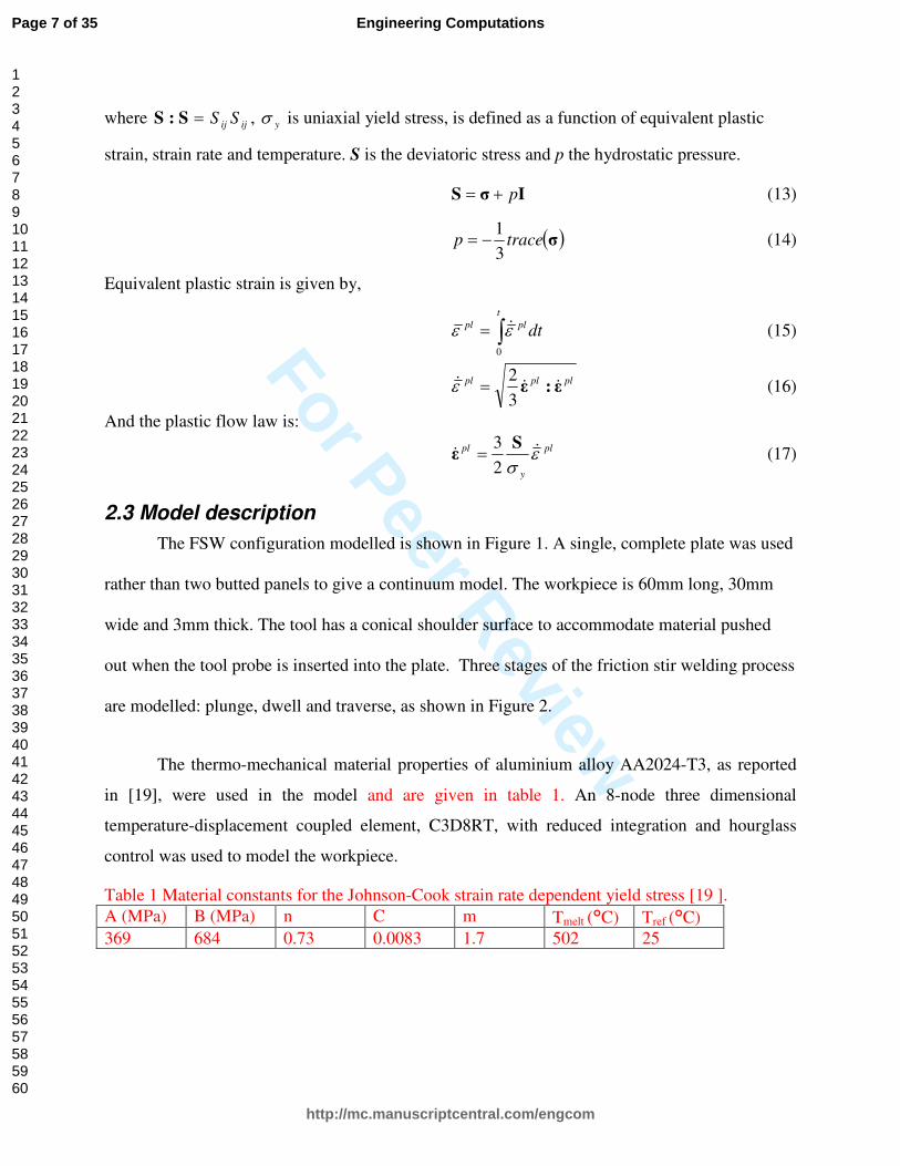
The thermo-mechanical material properties of aluminium alloy AA2024-T3, as reported

in [19], were used in the model and are given in table 1. An 8-node three dimensional

temperature-displacement coupled element, C3D8RT, with reduced integration and hourglass

control was used to model the workpiece.

Table 1 Material constants for the Johnson-Cook strain rate dependent yield stress [19 ]. A (MPa) B (MPa) n C m Tmelt (°C) Tref (°C) 369 684 0.73 0.0083 1.7 502 25

Page 7 of 35

http://mc.manuscriptcentral.com/engcom

Engineering Computations

123456789101112131415161718192021222324252627282930313233343536373839404142434445464748495051525354555657585960

For Peer Review

It was found that solution times for the model were very long and it was necessary to carry out a

mesh study [20] to choose a computationally economic mesh design for the model while

maintaining the quality of the mesh during deformation. A smaller plate was used instead of the

whole model to explore the effect of mesh size. Additionally only the plunge and dwell stages

were simulated in the mesh study. The number of elements through thickness and in horizontal

plane were varied. The typical solution time in the mesh study, for a single run, was 1 to 3 days

depending on the size of mesh used. For brevity a full description is not included here. Based on

the mesh study, the element size in the horizontal plane was chosen as 0.5mm x 0.5mm and 1mm

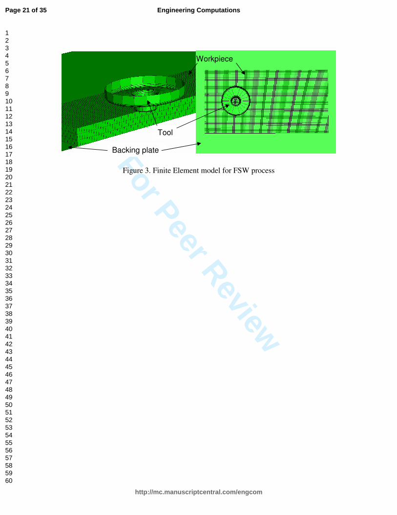
in thickness direction. The tool and backing plate were modelled as rigid isothermal surfaces, as

shown in figure 3. The total solution time for a full simulation of the FSW process, including

plunge, dwell and traverse stages, running on a PC with a 2.0 Ghz AMD Opteron Dual Core

processor, was 21 days and 6 hours .

The whole plate was defined as an adaptive domain, where the material can move

independently of the FE mesh. In the adaptive mesh domain, the top surface in contact with the

tool was defined as a sliding surface region, where the mesh follows the material movement in

the normal direction to the surface and moves independently of the underlying material in the

tangential direction.

Contacts between the tool and workpiece and between workpiece and backing plate were

simulated using the contact pair algorithm, as it is the only algorithm that can be used for coupled

thermo-stress analysis in ABAQUS/EPLICIT. At the tool-workpiece interface, Coulomb’s law of

friction is applied with a constant friction coefficient. At the backing plate-workpiece plate,

frictionless condition is assumed. The backing plate is fully fixed and the edges of bottom surface

of the workpiece are constrained so that no rigid body movement is allowed. A constant

temperature field equal to the environmental temperature is prescribed for the whole model at the

beginning of the analysis. All the surfaces of the workpiece were assumed to have convection

boundary conditions. The bottom surface in contact with backing plate has a convection

coefficient of 1000W/m2K, while the rest surfaces of the plate have a much lower convection

coefficient, 10 W/m2K [4].

Page 8 of 35

http://mc.manuscriptcentral.com/engcom

Engineering Computations

123456789101112131415161718192021222324252627282930313233343536373839404142434445464748495051525354555657585960

For Peer Review

The tool had a penetration speed of 0.25 mm/s and a plunging time of 8.3 seconds which

equates to a sinking depth of 0.075 mm. Following the plunge stage was the 0.1 second dwell

phase. This was found to be appropriate to generate a suitable temperature field and to keep the

welding material in a well-plasticized state so that a sound weld can be produced [7]. The

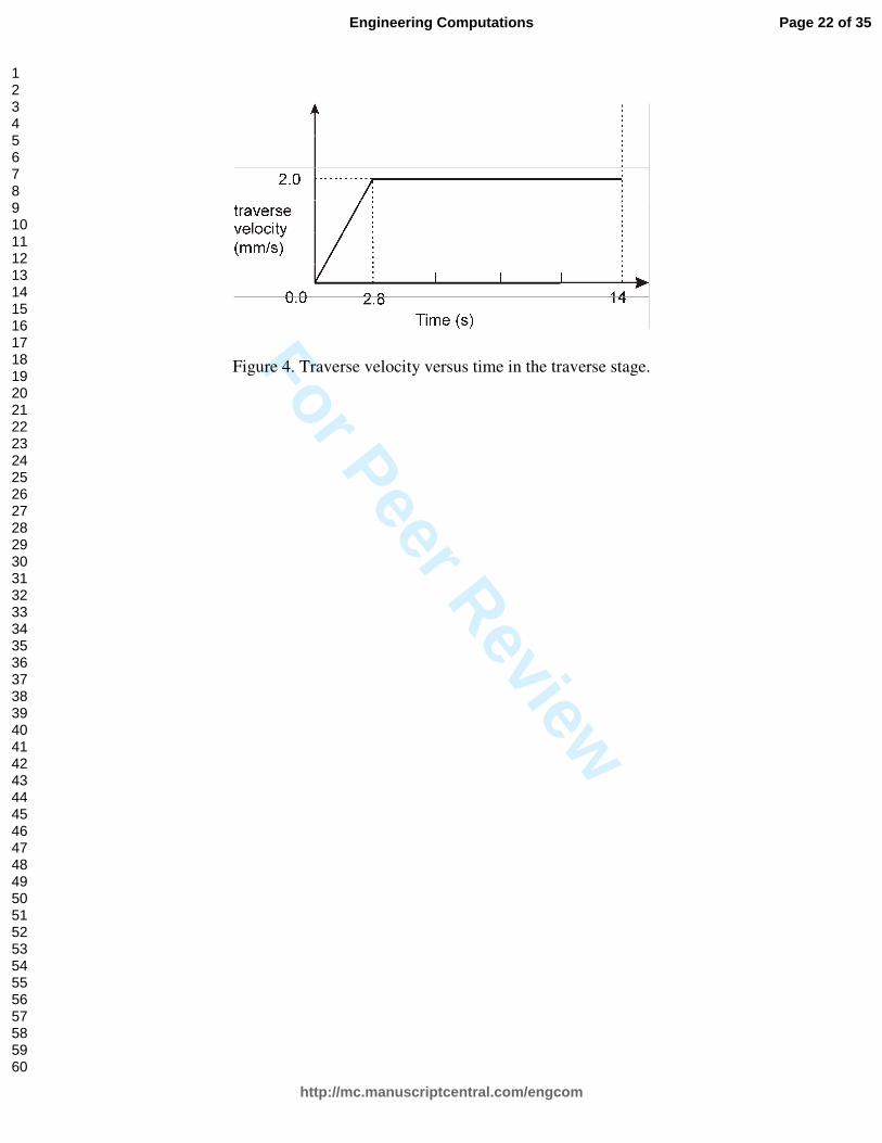
welding speed and welding time during the final traverse stage were set to 2 mm/s and 14

seconds, respectively.

To avoid sudden initial transverse movement of the tool (i.e. infinite acceleration at the onset of

welding) the traverse travelling speed was defined by a series of values at points in time in

ABAQUS, as shown in Figure 4.

3. Results

3.1 Temperature

The model can predict temperature evolution through the whole process and over the whole

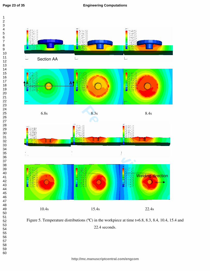
volume. Figure 5 shows the temperature distributions in degrees centigrade (ºC) at six

representative time points 6.8s, 8.3s, 8.4s, 10.4s, 15.4s and 22.4s. (Note plunge occurs from 0 to

8.34s, dwell occurs 8.3s to 8.4s and traverse occurs 8.4s to 22.4s) The top row pictures give the

cross-section views along the welding joint line while the bottom row pictures provide the views

from the top.

When only the pin was in contact with the workpiece, the maximum temperature in the

workpiece occurred somewhere adjacent to the edge of the pin bottom surface. At 6.8s the

shoulder surface started to contact the workpiece, thereafter, the maximum temperature moved

towards the corner between pin and shoulder surfaces. At 8.3s the full contact condition was

established between tool surface and top surface of the workpiece, where upon the maximum

temperature was around the shoulder-workpiece interface. A high temperature gradient with a

"basin" or “V” shape appeared in the workpiece beneath the tool demonstrating high heat flux

between the interface layer and workpiece's material outside the shoulder radius. After the 0.1s

dwelling, at 8.4s, the temperature was distributed more even between the leading side and trailing

side of the tool. Then the tool started to traverse to join the plates together. The welding process

quickly reached steady state and the temperature distribution pattern around the tool exhibited

little variation as displayed at 10.4s, 15.4s and 22.4s in Figure 5.

Page 9 of 35

http://mc.manuscriptcentral.com/engcom

Engineering Computations

123456789101112131415161718192021222324252627282930313233343536373839404142434445464748495051525354555657585960

For Peer Review

The temperature contour looks almost symmetric along the joint line on both the retreating and

advancing sides. This means the rotating motion of the tool will not significantly affect the

temperature distribution in the work piece.

The maximum temperature was found to be greater than melting point, which for this material

was 502ºC. The reason for this is possibly due to the nature of the assumed interaction between

the tool and workpiece. The tool was assumed to be rigid isothermal and had no temperature

DOF, there was no direct heat transfer between the tool and workpiece. Only a concentrated heat

capacity was specified and 20% of the total frictional energy was set to flow into the tool. The

remaining 80% of the frictional energy together with the plastic dissipation energy could possibly

account for the temperature in an element being greater than the melting point. In reality, the

fraction of frictional energy into the workpiece depends on the temperature and heat

conductivities in the tool and workpiece. The total frictional energy was calculated with a

constant friction coefficient, which is a function temperature and contact pressure. However the

most plausible reason is thought to do with mass scaling. During the simulation process, elements

near the tool typically experience large amounts of deformation (especially the plunge stage). The

reduced characteristic element length causes a smaller global time increment and therefore

increased solution time. Scaling the mass of these elements throughout the analysis can

significantly decrease the computation cost, a fixed mass factor, 10000 was chosen for the

coupled FSW model [20]. This significantly increased material density had changed the original

physical problem as the density is involved in both the mechanical and thermal governing

equations. However given that the final solution time for the model was 21 days and 6 hours,

mass scaling was deemed as a necessity to allow solution in a reasonable time frame.

3.2 Stress distribution

One of the most important features of the proposed model is the ability to predict the stress

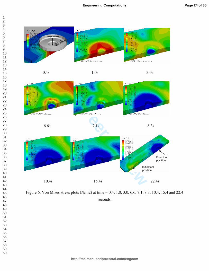
distributions (active stress and residual stress) over the whole FSW process. Figure 6 shows the

von Mises stress plots (N/m2) at nine characteristic time points, 0.4s, 1.0s, 3.0s, 6.6s, 7.1s, 8.3s,

10.4s, 15.4s and 22.4s from the start of the process. At the commencement of plunging, an axial

force was exerted on the material beneath the tool pin causing an area of high compressive stress

in the workpiece. With the growth of the heat at the pin-workpiece interface, the material

progressively softens. At 3.0s the stress in the plates under the tool pin nearly approached zero

Page 10 of 35

http://mc.manuscriptcentral.com/engcom

Engineering Computations

123456789101112131415161718192021222324252627282930313233343536373839404142434445464748495051525354555657585960

For Peer Review

caused by the extremely high temperature in this area, signified from the constitutive equations.

By 3.0 seconds the maximum stress migrated to somewhere remote from the pin-workpiece

interface. However at 6.6 seconds there was still a cylindrical layer of material surrounding the

tool pin that had fairly high stress as shown in the von Mises stress plot.

After the tool shoulder touched the workpiece at 6.8s, the cylindrical high stress layer gradually

disappeared since the material was heated up by the heat generated at the shoulder-pin interface.

At 8.3s most of the material under the tool was softened and in a state that it could be easily

stirred. During the welding stage, from 8.4s onwards, no obvious variation in the stress field

around the tool was found. This is due to the fact that the temperature distribution around the tool

after 8.4s reached a steady state as shown in Figure 5. From the observation of the stress

evolution throughout the process, it can be seen that the temperature imposes a significant effect

on the stress and consequently on the formation of the weld.

The last picture in Figure 6 shows the von Mises stress distribution at 22.4s. The maximum von

Mises stress in the region close to the starting position of the welding, increased from zero up to

270x106 N/m2. However the stress in the region nearer to the tool was quite low. This could be

the result of the small model used which is only 60 mm long and 30 mm wide. The temperature

was still very high over the whole plate at 22.4s as shown in the last picture of Figure 5. If the

workpiece cooled down it is expected that a distinctive residual stress could be identified along

the weld.

3.3 Plastic strain

The weld microstructure strongly depends on the thermal cycle and plastic deformation that the

material experienced. The ability of the model to calculate the plastic strain and strain rate makes

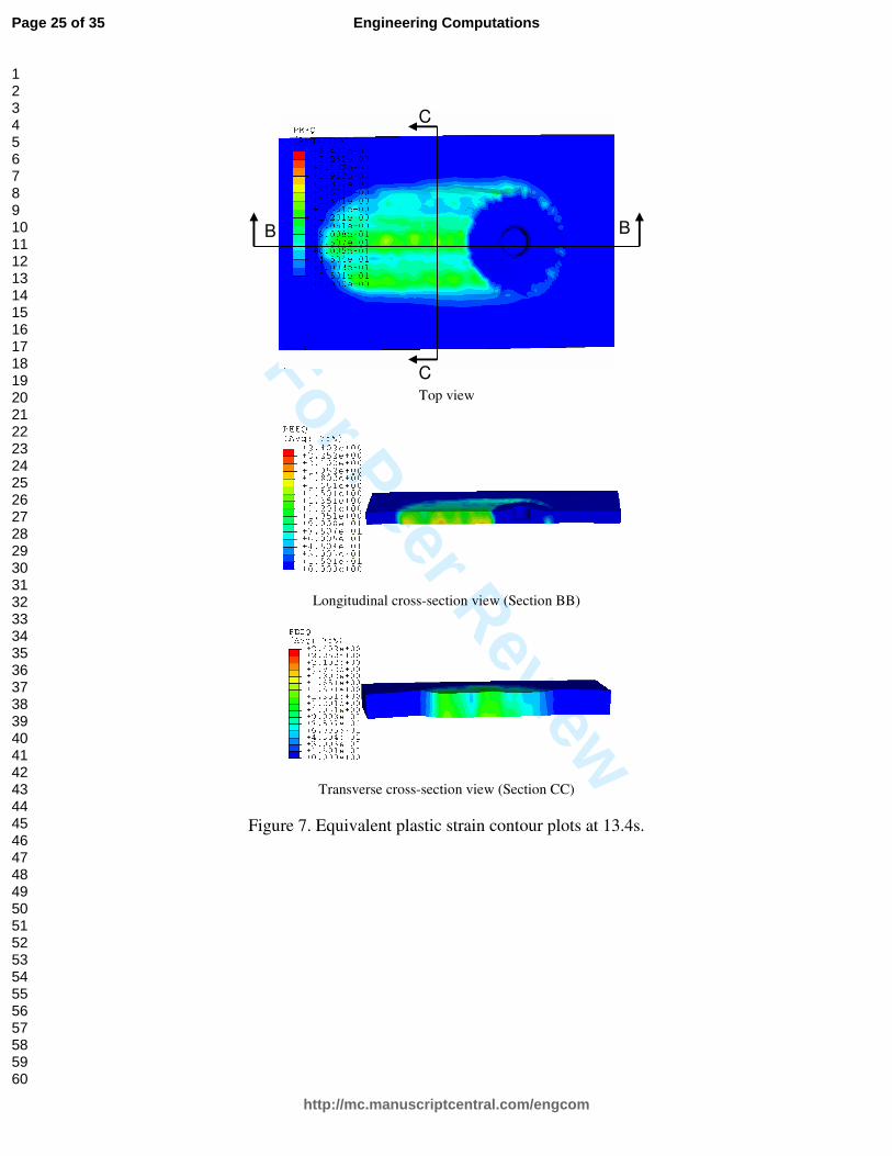
the prediction of the microstructure possible. In the present study only the plastic strain profile is

discussed. As an example, Figure 7 illustrates the equivalent plastic strain contour at 13.4s from

three perspectives, namely, top view, longitudinal cross section view (BB) and transverse cross-

section view (CC). It is apparent that the plastic strain distribution is not symmetric about the

joining line and the advancing side has a higher average plastic strain than the retreating side.

This is consistent with the findings in [7] and [21]. The highest plastic region is still along the

welding line with a width close to the pin diameter.

Page 11 of 35

http://mc.manuscriptcentral.com/engcom

Engineering Computations

123456789101112131415161718192021222324252627282930313233343536373839404142434445464748495051525354555657585960

For Peer Review

3.4 Tool reaction force and moment

Predicting the tool reaction force and moment is another distinctive feature of the current model.

Most of the 3D FE models in the literature can only compute the force in the welding stage when

the steady state has been established. However it is well known that the pin is subject to the

highest reaction forces in the plunge stage, as revealed in the experimental work [22]. The

considerable stresses that the pin experienced can lead to failure if the mechanical strength is not

sufficient. To prevent tool damage and improve its fatigue life, it is necessary to know,

reasonably accurately, the tool reaction forces and torque over the whole process.

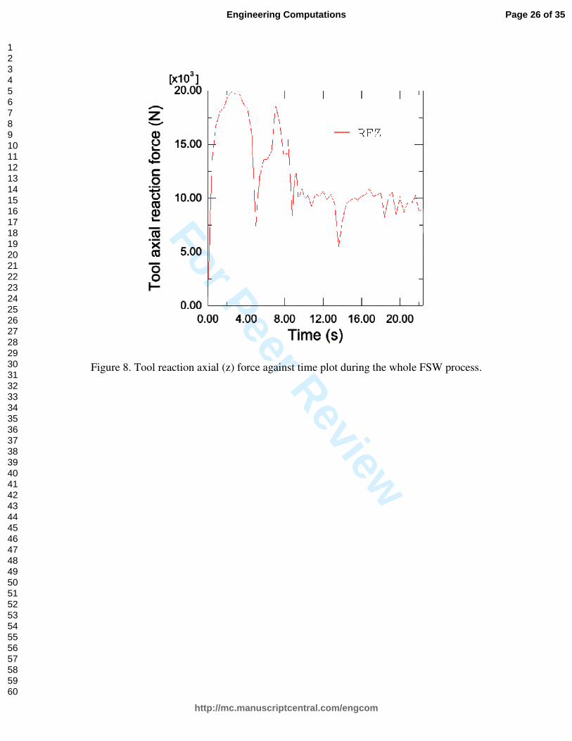
The variation of the tool axial (Z) reaction forces,RFZ, for the whole process is illustrated in

Figure 8. The plunge stage, at a constant speed, occurs during the first 8.3 seconds. The value of

the reaction forces in the transverse (X) and longitudinal (Y) directions are very small compared

with the axial (Z) reaction force and hence are not shown for brevity. The “RFZ” curve climbs

quickly for the first two seconds and then falls significantly to a low value at 5s. During the next

half second the curve suddenly increases again before reaching, at around 7s, a value just below

the previous maximum. This is followed by a period of gradual decrease with fluctuation. The

deep drop to a minimum at about 5s is thought due to the abrupt local material temperature

increment under the tool pin. As previously mentioned, the predicted temperature in the analysis,

was above the melting temperature for the material. Due to the overestimated temperature the

predicted force history in plunge stage probably requires further verification.

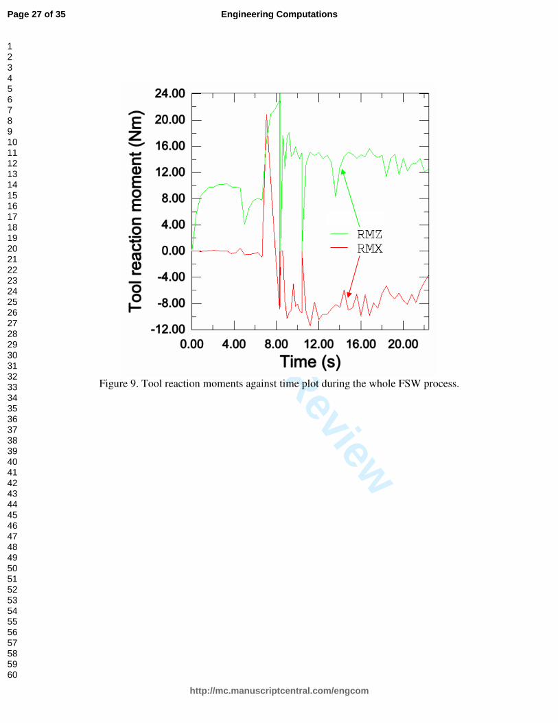
Figure 9 illustrates the variation of the tool reaction moments with time. “RMX” and “RMZ”

stand for the reaction moment components about the X and Z axis, respectively. The reaction

moment about the Y axis is small compared with the other two and not shown for clarity. At 6.8s

when the tool started to contact the workpiece, the curves jumped to its peak value which is much

higher than the previous maximum before 6.8s. After 8.4s in the dwell and traverse stages the

curve gradually decreases with fluctuation.

The fluctuation shown in figures 8 and 9 could suggest problems with stability in the numerical

solution possibly related to mass scaling.

Page 12 of 35

http://mc.manuscriptcentral.com/engcom

Engineering Computations

123456789101112131415161718192021222324252627282930313233343536373839404142434445464748495051525354555657585960

For Peer Review

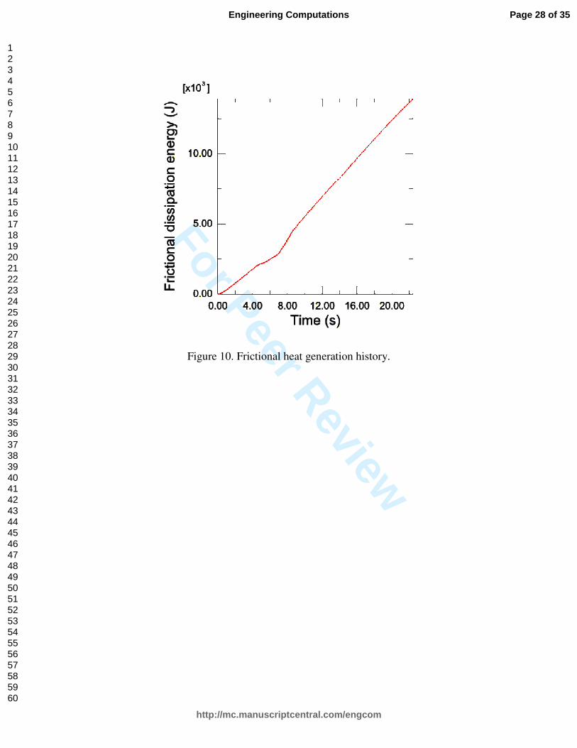
3.5 Heat generation

Heat generated from both friction and plastic deformation is plotted against time as shown in

Figures 10 and 11. Frictional energy dissipation and plastic dissipation increase in a bilinear

manner. There is a smooth transition region around 6s and generation rates become higher after

6.8s. In the current model results, friction was responsible for generating most of the heat needed

(98%) even when full contact condition had established and severe plastic deformation occurred,

indicating the sliding condition is dominant at the contact interface.

The model used a constant friction coefficient, 0.3 [4] and neglected its temperature dependence.

The surface interaction involving contact pressure, friction, temperature dependence etc, is very

complicated and at present is not fully understood. During the process, the friction force may also

cause the maximum yield shear stress in the workpiece material to be exceeded. The current

assumed contact condition is therefore far from the real situation. However due to the uncertainty

in the literature as to the nature of the surface interaction, it was decided, in this study as a first

step, to keep the contact model definition relatively simple. It is anticipated that a more complex

friction model, or one that at least considers the temperature effect, should give more accurate

results and the percentage of generated heat due to frictional effects will be expected to reduce.

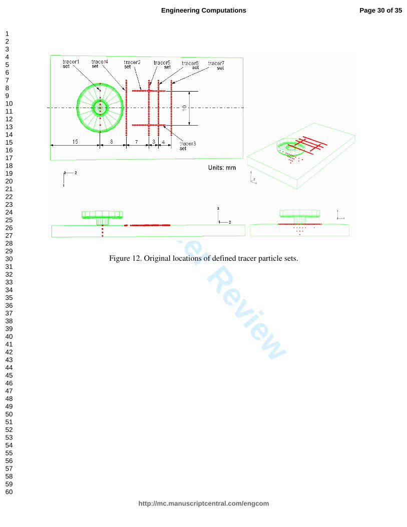
3.6 Material movement

The material flow during FSW is complicated and directly influences the properties of a FSW

weld. It is of vital importance to understand the deformation process and basic physics of the

material flow for optimal tool design. To visualize the material flow phenomenon, tracer particle

sets were defined symmetrically, each side, along the welding line to track the material

movement at specific locations. Seven tracer particle sets numbered 1 to 7, were used and

highlighted by the red points in Figure 12. Each tracer set includes a few particles in a line or/and

in a plane and their initial positions are clearly shown in the figure.

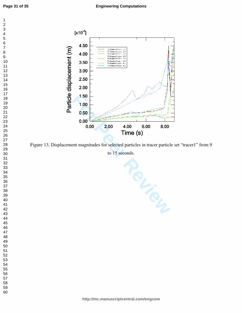
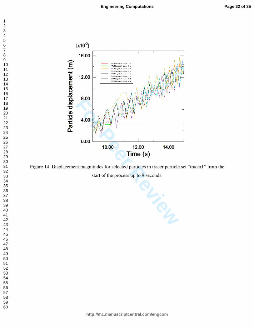
The displacement for several representative particles in tracer set “tracer1” is plotted in Figures

13 and 14. This tracer particle set was only defined in the first 15 seconds to reduce the size of

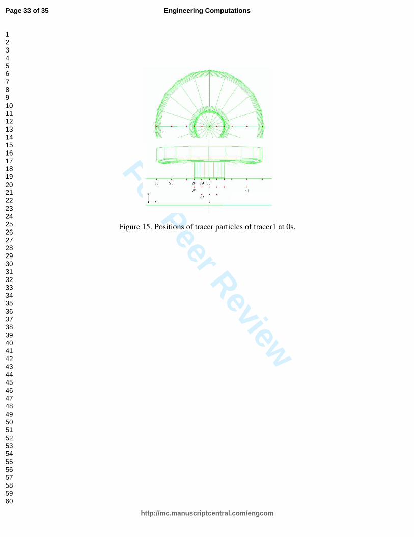
the results file. The selected particles are numbered in the Figure 15. The downward movement

of the tool was displacement controlled at a constant speed. This was reflected by the plot of the

Page 13 of 35

http://mc.manuscriptcentral.com/engcom

Engineering Computations

123456789101112131415161718192021222324252627282930313233343536373839404142434445464748495051525354555657585960

For Peer Review

displacement magnitude of tracer particle 30 which is directly under the centre of the tool, having

a linear straight line. Particle 28 at the edge of the pin was pushed aside when then pin started

plunging hence it had small displacement until stirred by the shoulder. Particle 29 which is also

below the pin bottom surface but with a distance of half a tool pin radius from the pin centre

experienced largest displacement (among all the tracer particles defined in current model) until

about 7.5 seconds, indicating this area of the material suffered most of the stir at the beginning of

the plunge. A quasi-linear increment was identified for particles remote from the intense stirring

zone. This could be explained as the result of global workpiece deformation. The workpiece was

fixed by constraining its bottom edge nodes, so when the tool pin was inserted into the workpiece

the material under the tool pin was pushed downwards and the workpiece outside the pin radius

bulged upwards. Particle 25, which was initially under the edge of tool shoulder, moved outside

the shoulder radius during tool penetration. From then on, it had no contact with the tool, thus its

displacement over the whole process was very small and purely due to the global workpiece

deformation, as illustrated by the red curve in Figures 13 and 14. There was no contact with the

tool either for particles 28, 36 and 42 before 7.8s, but once touched and stirred by the tool, the

displacement suddenly increased. A key time point can be identified at about 8.4s, after which all

the particles in contact with the tool experienced significant boost in displacement within a very

short period. At this moment, it could be said say that the material is in a flow state and ready for

welding.

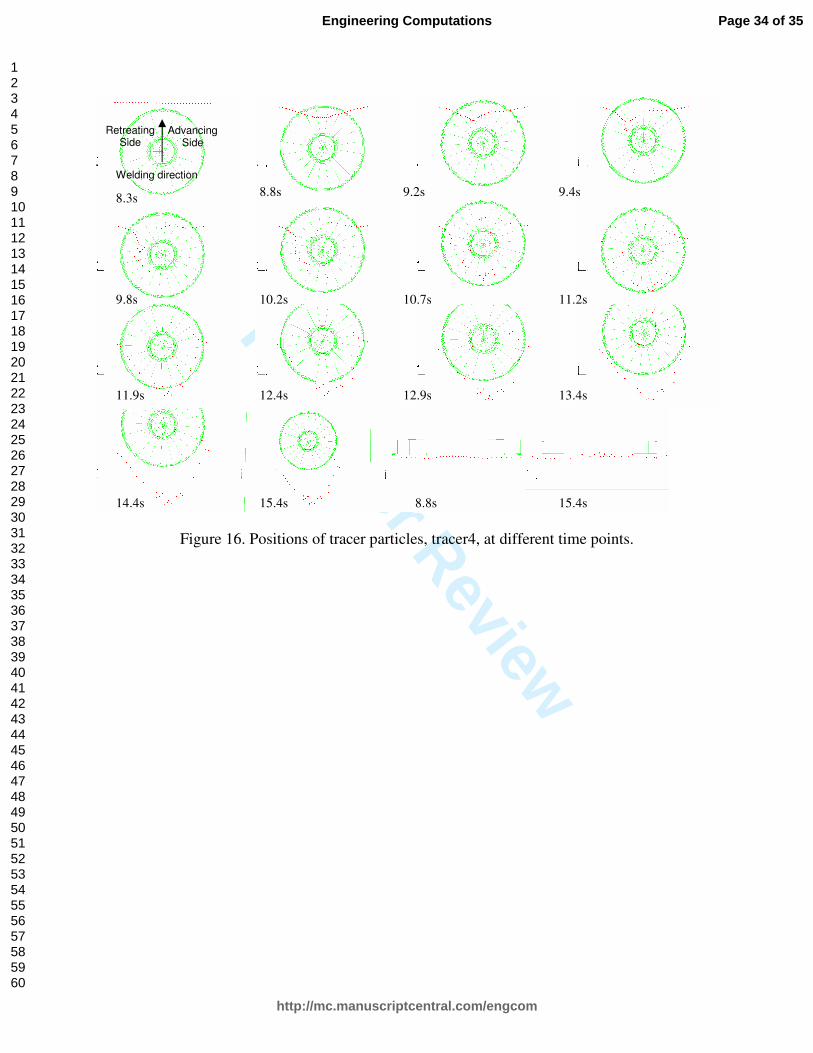
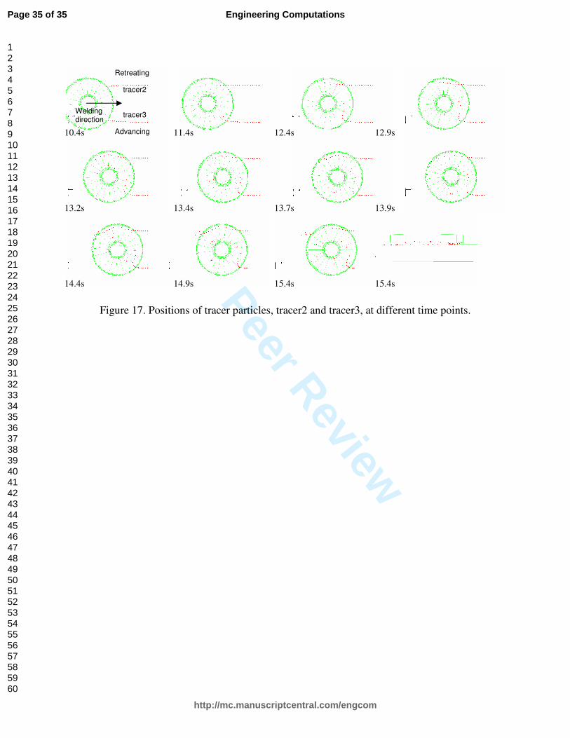
Figure 16 and Figure 17 demonstrate the particle locations of set tracer4 and set tracer2&3 at

several representative time points, respectively. The particle set tracer4 is a line of material points

in front of the tool perpendicular to the joining line (see Figure 16). While set tracer2 and set

tracer3 sit in separate lines along the welding direction, lying on the retreating side and advancing

side of the weld, respectively.

For set tracer4 the material points close to the centre line was first touched and sucked into the

conical shoulder-workpiece interface as shown in the pictures (top and cross-section views) of

Figure 16 at 8.8s (second from the left in top row and second from the right in bottom row). Then

the material points from advancing side were forced and squeezed to the retreating side, leading

to a non-symmetrical flow field. Most of the particles entering onto the retreating side under the

tool shoulder went through several revolutions and dropped off in the wake of the shoulder later

on, mainly on the advancing side. There were also some particles, primarily from retreating side,

Page 14 of 35

http://mc.manuscriptcentral.com/engcom

Engineering Computations

123456789101112131415161718192021222324252627282930313233343536373839404142434445464748495051525354555657585960

For Peer Review

at the contact interface that didn’t rotate with the shoulder. They remained on retreating side

when left behind by the tool. Finally the material particles formed an arc-shaped strip behind the

tool. This banded shape is already well known by numerous experimental studies in the literature

[23].

For set tracer2 in Figure 17 the particles entered shoulder-workpiece interface and rotated with

the shoulder only for a very short time. They were directly pushed back to the wake with the

advancing of the tool towards the welding direction. It is noted that the material particles never

flowed with the tool into the rotational zone. Again in Figure 17, tracer3 particles were stirred

into the rotational zone at various places and then sloughed off from the welding tool. Those

findings are consistent with observations in experiments [23-26]. Thus the ability of the model to

predict the material movement is well validated.

However, it should be noted that only a limited number of tracer particles were defined and the

flow on the top surface of the workpiece is dominated by the shoulder rather than by the pin. The

material has a quite different flow pattern at mid section and the lower part of the pin. To fully

track and study the material flow more tracer particles should be defined and seeded.

4. Conclusion

The multiphysics model proposed in this paper has successfully simulated the plunge, dwell and

traverse stages of the friction stir welding process. The development of field variables:

temperature, stress and plastic strain, are quantified by the model. The predicted maximum

temperature is higher than material melting point, resulting in a lower stress field than expected

around the tool during welding. Material movement is visualized by defining tracer particles at

the locations of interest. The numerically computed material flow patterns are in very good

agreement with the general findings in experiments.

In the future, the foremost model refinement work will involve lowering the predicted maximum

temperature values, by changing boundary conditions, mass scaling factors, heat partition

between the tool and workpiece. The fluctuations shown in some of the results could suggest

problems with stability in the numerical solution possibly related to mass scaling. This will be

investigated in future work.

Page 15 of 35

http://mc.manuscriptcentral.com/engcom

Engineering Computations

123456789101112131415161718192021222324252627282930313233343536373839404142434445464748495051525354555657585960

For Peer Review

Also the temperature dependent Young’s modulus, friction coefficient and shear stress limit can

lead to better temperature predictions.

To further study the material movement behavior at the tool-workpiece interface, more tracer

particles need to be seeded and parametric studies of process parameters will be performed.

References:

[1] Ulysse, P. (2002), “Three-dimensional Modelling of the Friction Stir-welding Process”, International Journal of Machine Tools & Manufacture, Vol. 42, pp. 1549-1557.

[2] FIDAP (1994), Fluid Dynamic Analysis Package, version 7.6, Fluid Dynamics International, Evanston, IL.

[3] Diego, H., Santiago, Lombera, F., Urquiza, S., Cassanelli, A. (2004), “Numerical Modeling of Welded Joints by the Friction Stir Welding Process”, Materials Research, Vol. 7, No. 4, pp. 569-574.

[4] Schmidt, H. and Hattel, J., (2005), “A Local Model for the Thermo-mechanical Conditions in Friction Stir Welding”, Modelling and Simulation in Materials Science and

Engineering, Vol. 13, pp. 77-93.

[5] ABAQUS/EXPLICIT (2006), Version 6.6-1, ABAQUS, Inc., Providence, USA.

[6] Forge 3 (2004), Release 6.3. Transvalor S.A.

[7] Buffa, G., Hua, J., Shivpuri, R., Fratini, L. (2006), “A Continuum Based Fem Model for Friction Stir Welding-Model Development”, Material Science and Engineering A, Vol. 419, Issues 1-2, pp. 389-396.

[8] DEFORM-3D, Scientific Forming Technologies Corporation (SFTC), Columbus, Ohio

[9] Lasley, M.J., (2005), “A Finite Element Simulation of Temperature and Material Flow in Friction Stir Welding”, Unpublished thesis, Brigham Young University, Provo, UT.

[10] Bendzsak, G.J., North, T.H. and Smith, C.B. (2000), “An experimentally validated 3D model for friction stir welding”, Proceedings of the Second International Symposium on

Friction Stir Welding, TWI Ltd., Gothenburg, Sweden.

[11] Colegrove, P., (2000), “Three Dimensional Flow and Thermal Modelling of the Friction Stir Welding Process”, Proceedings of the 2nd International Symposium on Friction Stir

Welding, Gothenburg, Sweden.

Page 16 of 35

http://mc.manuscriptcentral.com/engcom

Engineering Computations

123456789101112131415161718192021222324252627282930313233343536373839404142434445464748495051525354555657585960

For Peer Review

[12] Seidel, T.U. and Reynolds, A.P., “Two-dimensional Friction Stir welding Process Model Based on Fluid Mechanics”, Science and Technology of Welding & Joining, Vol. 8, No. 3, pp. 175-183.

[13] Askari, A., Silling, S., London, B., and Mahoney, M. (2001), Modeling and Analysis of

Friction Stir Welding Processes, the Minerals, Metals and Materials Society.

[14] Colegrove, P.A. and Shercliff, H.R (2005), “3-Dimensional CFD modelling of flow round a threaded friction stir welding tool profile”, Journal of Materials Processing

Technology, Vol. 169, No. 2, pp. 320-327.

[15] Sellars, C.M. and Tegart, W.J. (1972), “Hot Workability”, International Metallurgical

Review, 17, pp. 1–24.

[16] Nandan, R., Roy, G.G. and DebRoy, T. (2006), “Numerical Simulation of Three-Dimensional Heat Transfer and Plastic Flow During Friction Stir Welding”, Metallurgical

& Materials Transactions A, Vol. 37, pp. 1247–1259.

[17] Nandan, R., Roy, G.G., T. J. Lienert, and DebRoy, T. (2006), “Numerical Modelling of 3D Plastic Flow and Heat Transfer during Friction Stir Welding of Stainless Steel” Science and Technology of Welding & Joining, Vol. 11, No. 5, pp. 526-537.

[18] Nandan, R., Roy, G.G., T. J. Lienert, and DebRoy, T. (2007), “Three-dimensional Heat and Material Flow during Friction Stir Welding of Mild steel”, Acta Materialia, Vol. 55, pp. 883-895.

[19] Lesuer, D. R. (2000), Technical Report FAA and DOE, USA [20] Hongjun Li, (2008), "Coupled Thermo-Mechanical Modelling of Friction Stir Welding

Process", PhD Thesis, Univ. of Strathclyde.

[21] Heurtier, P., Desrayaud, C., and Montheillet, F. (2002), "A Thermomechanical Analysis of the Friction Stir Welding Process", Materials Science Forum, Vol. 396, No. 4, pp. 1537-1542.

[22] Lienert T.J., Stellwag W.L. Jr., Grimmett, B.B., and Warke, R.W., (2003), “Friction Welding Studies on Mild Steel”, Supplement to the Welding Journal, Vol. 82(1), pp. 1s-9s.

[23] Seidel, T.U. and Reynolds, A.P. (2001), “Visualization of the Material Flow in AA2195 Friction-Stir Welds Using a Marker Insert Technique”, Metallurgical and materials

Transactions A, Vol. 32, pp. 2879.

[24] Schmidt, H.N.B., Dickerson, T.L. and Hattel, J.H. (2006), “Material flow in butt friction stir welds in AA2024-T3”, Acta Materialia, Vol. 54, pp. 1199-1209.

[25] Reynolds, A.P. (2000), “Visualisation of material flow in autogenous friction stir welds”, Science and Technology of Welding & Joining, Vol. 5, No. 2, pp. 120-124.

Page 17 of 35

http://mc.manuscriptcentral.com/engcom

Engineering Computations

123456789101112131415161718192021222324252627282930313233343536373839404142434445464748495051525354555657585960

For Peer Review

[26] Mishra, R.S. and Ma, Z.Y. (2005), “Friction stir welding and processing”, Materials

Science and Engineering: R: Reports, Vol. 50, No. 1-2, pp. 1-78.

Page 18 of 35

http://mc.manuscriptcentral.com/engcom

Engineering Computations

123456789101112131415161718192021222324252627282930313233343536373839404142434445464748495051525354555657585960

For Peer Review

Figure 1. FSW model geometry (in mm)

X

Y

Page 19 of 35

http://mc.manuscriptcentral.com/engcom

Engineering Computations

123456789101112131415161718192021222324252627282930313233343536373839404142434445464748495051525354555657585960

For Peer Review

Figure 2. The three stages of FSW simulated in the FE model

Page 20 of 35

http://mc.manuscriptcentral.com/engcom

Engineering Computations

123456789101112131415161718192021222324252627282930313233343536373839404142434445464748495051525354555657585960

For Peer Review

Figure 3. Finite Element model for FSW process

Tool

Backing plate

Workpiece

Page 21 of 35

http://mc.manuscriptcentral.com/engcom

Engineering Computations

123456789101112131415161718192021222324252627282930313233343536373839404142434445464748495051525354555657585960

For Peer Review

Figure 4. Traverse velocity versus time in the traverse stage.

Page 22 of 35

http://mc.manuscriptcentral.com/engcom

Engineering Computations

123456789101112131415161718192021222324252627282930313233343536373839404142434445464748495051525354555657585960

For Peer Review

6.8s 8.3s 8.4s

10.4s 15.4s 22.4s

Figure 5. Temperature distributions (ºC) in the workpiece at time t=6.8, 8.3, 8.4, 10.4, 15.4 and

22.4 seconds.

Section AA

A A

Welding direction

Page 23 of 35

http://mc.manuscriptcentral.com/engcom

Engineering Computations

123456789101112131415161718192021222324252627282930313233343536373839404142434445464748495051525354555657585960

For Peer Review

0.4s 1.0s 3.0s

6.6s 7.1s 8.3s

10.4s 15.4s 22.4s

Figure 6. Von Mises stress plots (N/m2) at time = 0.4, 1.0, 3.0, 6.6, 7.1, 8.3, 10.4, 15.4 and 22.4

seconds.

Initial tool

position

Final tool

position

Page 24 of 35

http://mc.manuscriptcentral.com/engcom

Engineering Computations

123456789101112131415161718192021222324252627282930313233343536373839404142434445464748495051525354555657585960

For Peer Review

Top view

Longitudinal cross-section view (Section BB)

Transverse cross-section view (Section CC)

Figure 7. Equivalent plastic strain contour plots at 13.4s.

B B

C

C

Page 25 of 35

http://mc.manuscriptcentral.com/engcom

Engineering Computations

123456789101112131415161718192021222324252627282930313233343536373839404142434445464748495051525354555657585960

For Peer Review

Figure 8. Tool reaction axial (z) force against time plot during the whole FSW process.

Page 26 of 35

http://mc.manuscriptcentral.com/engcom

Engineering Computations

123456789101112131415161718192021222324252627282930313233343536373839404142434445464748495051525354555657585960

For Peer Review

Figure 9. Tool reaction moments against time plot during the whole FSW process.

Page 27 of 35

http://mc.manuscriptcentral.com/engcom

Engineering Computations

123456789101112131415161718192021222324252627282930313233343536373839404142434445464748495051525354555657585960

For Peer Review

Figure 10. Frictional heat generation history.

Page 28 of 35

http://mc.manuscriptcentral.com/engcom

Engineering Computations

123456789101112131415161718192021222324252627282930313233343536373839404142434445464748495051525354555657585960

For Peer Review

Figure 11. Plastic deformation heat generation history.

Page 29 of 35

http://mc.manuscriptcentral.com/engcom

Engineering Computations

123456789101112131415161718192021222324252627282930313233343536373839404142434445464748495051525354555657585960

For Peer Review

Figure 12. Original locations of defined tracer particle sets.

Page 30 of 35

http://mc.manuscriptcentral.com/engcom

Engineering Computations

123456789101112131415161718192021222324252627282930313233343536373839404142434445464748495051525354555657585960

For Peer Review

Figure 13. Displacement magnitudes for selected particles in tracer particle set “tracer1” from 9

to 15 seconds.

Page 31 of 35

http://mc.manuscriptcentral.com/engcom

Engineering Computations

123456789101112131415161718192021222324252627282930313233343536373839404142434445464748495051525354555657585960

For Peer Review

Figure 14. Displacement magnitudes for selected particles in tracer particle set “tracer1” from the

start of the process up to 9 seconds.

Page 32 of 35

http://mc.manuscriptcentral.com/engcom

Engineering Computations

123456789101112131415161718192021222324252627282930313233343536373839404142434445464748495051525354555657585960

For Peer Review

Figure 15. Positions of tracer particles of tracer1 at 0s.

Page 33 of 35

http://mc.manuscriptcentral.com/engcom

Engineering Computations

123456789101112131415161718192021222324252627282930313233343536373839404142434445464748495051525354555657585960

For Peer Review

Figure 16. Positions of tracer particles, tracer4, at different time points.

8.3s 8.8s

8.8s 15.4s 15.4s

9.2s 9.4s

9.8s 10.2s 10.7s 11.2s

11.9s 12.4s 12.9s 13.4s

14.4s

Retreating

Side

Advancing

Side

Welding direction

Page 34 of 35

http://mc.manuscriptcentral.com/engcom

Engineering Computations

123456789101112131415161718192021222324252627282930313233343536373839404142434445464748495051525354555657585960

For Peer Review

Figure 17. Positions of tracer particles, tracer2 and tracer3, at different time points.

10.4s 11.4s 12.4s 12.9s

13.2s 13.4s 13.7s 13.9s

14.4s 14.9s 15.4s 15.4s

Advancing

tracer2

tracer3

Retreating

Welding

direction

Page 35 of 35

http://mc.manuscriptcentral.com/engcom

Engineering Computations

123456789101112131415161718192021222324252627282930313233343536373839404142434445464748495051525354555657585960