Multi-performance Target Collaborative Optimization Methods for Battery Electric Vehicle Chen Yawei Chongqing Jiaotong University Chen Qian Chongqing Jiaotong University Liu Jurui ji lin jian zhu gong cheng xue yuan: Jilin Jianzhu University Hao Xixiang Chongqing Jiaotong University Yuan Chenheng ( [email protected] ) Chongqing Jiaotong University https://orcid.org/0000-0003-4376-8194 Original Article Keywords: Battery Electric Vehicle (BEV), Multi-objective Optimization, Pareto Optimum Principle, 19 Evolutionary Algorithm Posted Date: September 20th, 2021 DOI: https://doi.org/10.21203/rs.3.rs-895705/v1 License: This work is licensed under a Creative Commons Attribution 4.0 International License. Read Full License

Welcome message from author
This document is posted to help you gain knowledge. Please leave a comment to let me know what you think about it! Share it to your friends and learn new things together.
Transcript

Multi-performance Target CollaborativeOptimization Methods for Battery Electric VehicleChen Yawei
Chongqing Jiaotong UniversityChen Qian
Chongqing Jiaotong UniversityLiu Jurui
ji lin jian zhu gong cheng xue yuan: Jilin Jianzhu UniversityHao Xixiang
Chongqing Jiaotong UniversityYuan Chenheng ( [email protected] )
Chongqing Jiaotong University https://orcid.org/0000-0003-4376-8194
Original Article
Keywords: Battery Electric Vehicle (BEV), Multi-objective Optimization, Pareto Optimum Principle, 19Evolutionary Algorithm
Posted Date: September 20th, 2021
DOI: https://doi.org/10.21203/rs.3.rs-895705/v1
License: This work is licensed under a Creative Commons Attribution 4.0 International License. Read Full License

1
Multi-performance Target Collaborative Optimization Methods for 1
Battery Electric Vehicle 2
Yawei Chen1, Qian Cheng
1, Jurui Liu
2, Xixiang Hao
3 Chenheng Yuan
4,* 3
Abstract: The present studies on battery electric vehicles (BEVs) has mainly focused on the single-objective 4
or weighted multi-objective optimization based on energy management, which can not manifest the coupling 5
relationship among the vehicle performance objectives essentially. To optimize the handling stability, ride comfort 6
and economy of BEV, this paper built the stability dynamics analysis model, ride comfort simulation half-car 7
model and power consumption calculation model of BEV, as well as two-point virtual random excitation model on 8
Level B road and proposed related evaluation indexes, including vehicle handling stability factor, weighted 9
acceleration root-mean-square (RMS) value of vertical vibration at the driver’s seat and power consumption per 10
100 m at a constant speed. The Pareto optimum principle–based multi-objective evolutionary algorithm (MOEA) 11
of BEV was also designed, which was encoded with real numbers and obtained the target values of all optional 12
schemes via MATLAB/Simulink simulation software. The merits and demerits of alternative schemes could be 13
judged according to the Pareto dominance principle, so that alternative schemes obtained after optimization were 14
realizable. The results of simulation experiment suggest that the proposed algorithm can perform the 15
multi-objective optimization on BEV, and obtain a group of Pareto optimum solutions featured by high handling 16
stability, favorable ride comfort and low energy consumption for the decision-makers. 17
Keywords: Battery Electric Vehicle (BEV); Multi-objective Optimization; Pareto Optimum Principle; 18
Evolutionary Algorithm 19
20 1 21
1 *Corresponding author E-mail: [email protected] (C. Yuan) 4Chongqing Jiaotong University College of Traffic & Transportation, Chongqing 400074, China.
Full list of author information is available at the end of the article

2
0 Introduction 22
The efficient operation of BEV entails the coordination of handling stability, ride comfort and economy, with 23
non-differentiable, discontinuous, hybrid, multidimensional, constrained and nonlinear characteristics in its mocel, 24
which is a typical hybrid nonlinear multi-objective optimization issue. Els et al. optimized the suspension 25
characteristic parameters with dynamic-Q algorithm, for the multi-objective optimization of vehicle handling 26
stability and ride comfort, and provided a set of suspension parameters which can improve vehicle handling 27
stability and ride comfort for decision makers [1]
. Yang Guangci et al. optimized the fuel consumption, HC+NOx 28
emissions and CO emissions of hybrid electric vehicle (HEV), and proposed a multi-objective optimization 29
evolutionary algorithm based on the Pareto optimum principle for HEV, thus obtaining the Pareto optimum 30
solution set with low fuel consumption and low emissions [2]
. Zhang Jingmei et al. improved the genetic algorithm 31
to realize the multi-objective comprehensive optimization of ride comfort, handling stability and road-friendliness 32
of vehicles, and obtained the best matching value of suspension stiffness and damping [3]
. Yang Rongshan et al. 33
balanced and optimized handling stability and ride comfort of vehicles with approximate model, and then obtained 34
the optimum value of suspension stiffness, damping and stabilizer bar [4]
. Ding Xiaolin et al. proposed a 35
multi-objective optimization matching method for driving system parameters, to improve the ride comfort of 36
four-hub motor-driven electric vehicles and reduce the energy consumption [5]
. Song Kang et al. conducted the 37
optimized analysis on suspension and seat parameters based on ride comfort of vehicles, and built a 38
multi-objective optimization model of vehicle dynamic performance. Non-dominated sorting genetic algorithm 39
(NSGA-II) with elite strategy was selected to solve the optimization model, and the Pareto optimum solution set 40
and Pareto frontier were obtained [6]
. Chen Yikai et al. determined the optimum control parameters to make road 41
friendliness and ride comfort of vehicles comprehensively through range and variance analysis, in order to 42
improve road friendliness and ride comfort of vehicles at the same time. The simulation results show that the 43

3
multi-objective optimum control strategy can make the vehicle comfortable and robust to the change of pavement 44
grade [7]
. Zhang Zhifei et al. took the vertical acceleration of the driver and the frame and the sum of the 95th 45
percentile to the fourth power as the performance optimization indexes, to normalize the weight of indexes to a 46
single-objective function by analytic hierarchy process for improving ride comfort and road friendliness of 47
commercial vehicles, as well as optimizing the stiffness and damping of suspension by genetic algorithm. The 48
simulation results show that ride comfort and road friendliness of optimized vehicles are improved effectively [8]
. 49
Yang Kun et al. conducted parameter sensitivity analysis on ride comfort and road friendliness of six-axle 50
semitrailer with the optimal Latin hypercube experimental design method, selected appropriate parameters 51
combined with the actual situation and optimized ride comfort, road friendliness, the comprehensive performance 52
of ride comfort and road friendliness with neighborhood cultivated multi-objective genetic optimization 53
algorithm. The research results show that under the common driving speed, the evaluation indexes of selected 54
optimization scheme, smoothness and road friendliness can also be better optimized [9]
. Zhou Feikun et al. carried 55
out multi-objective optimization on parameter matching of dynamical system with the optimization method of 56
SAPSO with average mileage under multiple working conditions, average total energy consumption under 57
multiple working conditions and complete vehicle kerb mass as the specific targets. The simulation results show 58
that the weight of vehicles can be reduced and the economic performance on the premise of ensuring the dynamic 59
performance can be improved [10]
. Zhang Kangkang et al. compared and selected the 3 dynamical system 60
matching projects with maximum speed, acceleration time and power consumption per 100 km as the specific 61
targets, solved the problem of conflicting among indexes to be optimized with the multi-objective genetic 62
algorithm, described the competitive relationship between indexes with the Pareto matrix, and clearly defined the 63
constraints and scope of application of policies [11]
. 64
Most of the above studies transformed the multi-objective optimization to single-objective optimization 65
through weighting or other methods, and then obtained the solution through mathematical programming. 66

4
Therefore, they have the following weaknesses: (1) The decision-makers were needed to provide profound 67
preference knowledge (i.e. weight coefficient of each target), to build single-objective evaluation function; (2) A 68
majority of single-objective optimization technologies were based on local optimization search algorithm. Despite 69
the local or global optimum solution obtained for single-objective optimization, several optimum solutions that 70
are available couldn’t be searched concurrently, thus, the flexible requirements of multi-objective decision can be 71
hardly met. 72
In addition, most of the optimization objectives in the researches on single-objective or multi-objective 73
optimization were vehicle handling stability or ride comfort but the researches about the multi-performance target 74
collaborative optimization of handling stability, ride comfort and economy of BEVs could be seldom found. For 75
this reason, this paper built the stability dynamics analysis model, the ride comfort simulation half-car model and 76
the power consumption calculation model, as well as the two-point virtual random excitation model of Level B 77
road surface, respectively, with BEV as the research object, and proposed the evaluation indexes corresponding to 78
the multi-performance objectives by highlighting the multi-objective optimization of BEVs’ handling stability, 79
ride comfort and economy under the turning condition, with simulation verification on handling stability, ride 80
comfort and economy of BEVs based on Pareto optimal algorithm. The simulation results show that the proposed 81
Pareto optimal algorithm can collaboratively optimize the safety, ride comfort and economy of BEVs, with the 82
improvement of handling stability, ride comfort and economy to a certain extent. 83
The innovation points of this paper include: 1) Based on the improved optimization algorithm of 84
non-dominated genetic algorithm, the elite strategy was introduced, with congestion distance and its comparison 85
operator as the basis of secondary sorting. Finally, the global optimal Pareto optimum solution and Pareto front 86
edge were obtained. 2) With handling stability, ride comfort and economy of BEVs as optimization objectives for 87
the first time, the key parameters related to multiple performance were selected as design parameters, to realize 88
the multi-objective optimization of dynamical performance of BEVs, and the optimal matching scheme of several 89
5
key parameters was obtained. 3) The optimization ideas and methods have important theoretical significance and 90
engineering practical application value for the optimization design of multi-objective parameters including other 91
mechanical properties of BEVs, such as handling stability transient response analysis and transmission 92
performance. 93
1 Vehicle Dynamics Models 94
1.1 Vehicle Dynamics Half-car Model 95
Vehicles receive inputs from longitudinal, vertical, and transverse directions, from which, the motion 96
response characteristics are definitely interactive and coupled mutually. The influence of vertical coupling motion 97
generated by the listing under the working condition of uniform turning movement on the vertical comfort of the 98
driver can be ignored. Therefore, this paper considered the vertical motion of vehicles alone when building ride 99
comfort model. First of all, the complex vehicle system was properly simplified and assumed: 100
1) Vehicles are symmetrical to the longitudinal symmetry plane and road unevenness corresponding to the 101
four tires is the same; 2) It is assumed that the road unevenness conforms to the normal distribution of each state 102
after a stationary random process, the road unevenness corresponding to each tire on the same side is different, 103
with a response time delay caused by the wheelbase; 3) Both the stiffness of tires and seats are simplified into 104
linear function; Suspension damping is a linear function of speed; 4) Each tire has a single contact with the 105
ground , without any bounce; Road excitation acts on the central point of contact between tires and the road 106
surface.. 107
After linearizing the automobile system into a half simplified model approximately, front and rear tires will 108
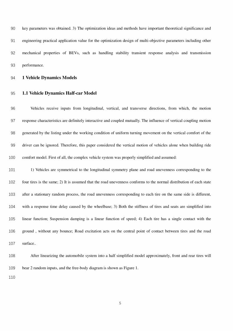
bear 2 random inputs, and the free-body diagram is shown as Figure 1. 109
110
6
111
Figure 1 Vehicle 4-DOF Model 112
All parameters in Figure 1 are set as follows: 𝑚𝑏 is curb weight; 𝐼𝑏 is vehicle turning inertia; 𝑚𝑓 and 𝑚𝑟 113
are unsprung mass of front suspension and rear suspension, respectively; 𝐾𝑐1 and 𝐶𝐶1 are spring stiffness and 114
damping of driver seat, respectively; 𝐾𝑓 and 𝐶𝑓 are spring stiffness and damping of front suspension, 115
respectively; 𝐾𝑟 and 𝐶𝑟 are spring stiffness and damping of rear suspension, respectively; 𝐾𝑡𝑓 and 𝐶𝑡𝑓 are 116
stiffness and damping of front tires, respectively; 𝐾𝑡𝑟 and 𝐶𝑡𝑟 are stiffness and damping of rear tires, respectively; 117
𝑞𝑓 and 𝑞𝑟 are vertical displacement excitation of front and rear tires, respectively. 118
According to D'Alembert’s principle, the differential equation of vibration motion of 4-DOF can be 119
expressed as: 120
0q qMZ CZ KZ C Q K Q (1) 121
Where, 𝑍 = [𝑍1, 𝑍𝑏 , 𝑍𝑐 , 𝑍𝑠]𝑇; 𝑍𝑠, 𝑍𝑏,𝑍1 and 𝑍𝑐 are vertical vibration displacement of driver seat, vehicle 122
body, front suspension and rear suspension, respectively; 𝑀 is mass matrix; 𝐶 is system damping matrix; 𝐾 is 123
system stiffness matrix; 𝐾𝑞 is road excitation stiffness; and 𝑄 is road excitation displacement. According to 124
Literature [12], the linear inhomogeneous equation set of 4 frequency response functions within the range of 125
frequency domain can be obtained from Formula (1): 126
6 6 1 2 3 4
1 2 3 4
T
T
A H H H H
Q Q Q Q
(2) 127
𝐴6×6 is the response coefficient matrix of each response frequency. It has been verified that its rank is 128
ZbZs
Ms
Kc1Cc1 mb
cz
KfCf
mfZ1
qfCtf
Ktf
KrCr
mr
KtrCtr
qr

7
related to its augmented matrix 𝐵4×5, so the equation set has a solution. In the formula, [𝐻1 𝐻2 𝐻3 𝐻4] 129
correspond to 4 vibration responses relative to the frequency response function vector of the front tire random 130
excitation input [𝐻𝑧1−�̃�𝑓 , 𝐻𝑧𝑏−�̃�𝑓, 𝐻𝑧𝑐−�̃�𝑓 𝑎𝑛𝑑 𝐻𝑧𝑠−�̃�𝑓]𝑇, and the frequency response function of seat acceleration 131
can be finally obtained. 132
1.2 Handling Stability Model 133
Handling stability of vehicles when driving mainly includes longitudinal stability and lateral stability. 134
Longitudinal stability may be out of control mainly in course of longitudinal driving on slope. Lateral stability is 135
mainly reflected in the form of cross slip or rollover. Listing motion is produced when vehicle makes a turn at a 136
uniform speed and the vehicle inclination leads to lateral deformation of the suspension system. The complete 137
vehicle model simplified into a 2-DOF system with lateral oscillation rotating z axis and lateral motion rotating y 138
axis alone is shown in Figure 2 [13]
. Then, vehicle listing dynamics model was established, i.e., the relation 139
between the listing stability factor, the listing characteristics of suspension and the dynamic load generated by the 140
road random excitation. 141
142
Figure 2 Vehicle Model of 2-DOF 143
In Figure 2, 𝛼1 and 𝛼2 are slip angle of front and rear tires; 𝛽 is slip angle of vehicle centroid; 𝛿 is front 144
wheel angle; 𝜔𝑟 is speed of heading angle; 𝑚 is total weight of vehicles; 𝐼𝑧 is rotational inertia of vehicle 145
rotating z axis; 𝑎 and 𝑏 are the distance from front axis and rear axis to vehicle centroid, respectively; 𝑢 and 𝑣 146
y
bu
Vv
m, IZ
a
a1
a2
L
x
'O
r

8
are weight of speed 𝑉 of vehicle centroid on 𝑥 axis and 𝑦 axis. 147
Supposed that vehicle vertical displacement and lateral displacement are all zero, the systematic differential 148
equation of motion can be expressed as below by ignoring the influence of suspension temporarily under the input 149
of front wheel, and considering the planar motion of vehicle alone. 150
1 2 1 2 1
1( ) ( ) ( )r rk k ak bk k m u
u (3) 151
2 2
1 2 1 2 1
1( ) ( ) r Z rak bk a k b k ak I
u (4) 152
When the vehicle is moving at a constant circular motion type, �̇�𝑟 = 0 and �̇� = 0, and the vehicle steering 153
sensitivity, 𝛾 = 𝜔𝑟/𝛿, can be obtained. 𝑘1 and 𝑘2 are the cornering stiffness of front and rear tires, respectively. 154
According to Formula (3) and Formula (4), stability factor can be expressed as: 155
2
2 1
m a bK
L k k
(5) 156
The tire cornering stiffness is closely related to the tire vertical load, which can be expressed as: 157
2
( ) ( ) ( )0.06778 9.144 5.129il r zil r zil rk F F (6) 158
Where, 𝐹′𝑧𝑖𝑙(𝑟) is the tire load of front and rear axles, respectively. 𝑙 and 𝑟 mean the left side and the right 159
side. 160
( ) ( ) ( ) 1,2zil r zil r zil r idF F F F i (7) 161
Where, 𝐹𝑧𝑖𝑙(𝑟) is the vertical reaction force of ground of front and rear axles and left (right) tire under an 162
idle status. The amount of change of vertical load includes two parts: 𝐹𝑖𝑑, i.e., the dynamic load applied to front 163
and rear axles respectively by road random excitation and ∆𝐹𝑧𝑖𝑙(𝑟), the amount of change of vertical reaction 164
applied to front and rear axles and left (right) tire by the centrifugal force. Therefore, the improved stability factor 165
can be expressed as: 166
( ) 2
2 ( ) 1 ( )
l r
l r l r
m a bK
L k k
(8) 167

9
2 Two-point Virtual Random Excitation Model of Road Surface 168
The road excitation born by vehicles in driving belongs to multiple-support excitation. In consideration of the 169
large wheel base, front and rear tires have receive stable and hysteresis road excitation of different phrases. A road 170
model is built within the frequency domain by taking Level B road surface as an example [14]
. Suppose that front 171
and rear tires receive the same related stable road excitation, the two excitation points of road surface can be 172
expressed as: 173
11
( )
22
t
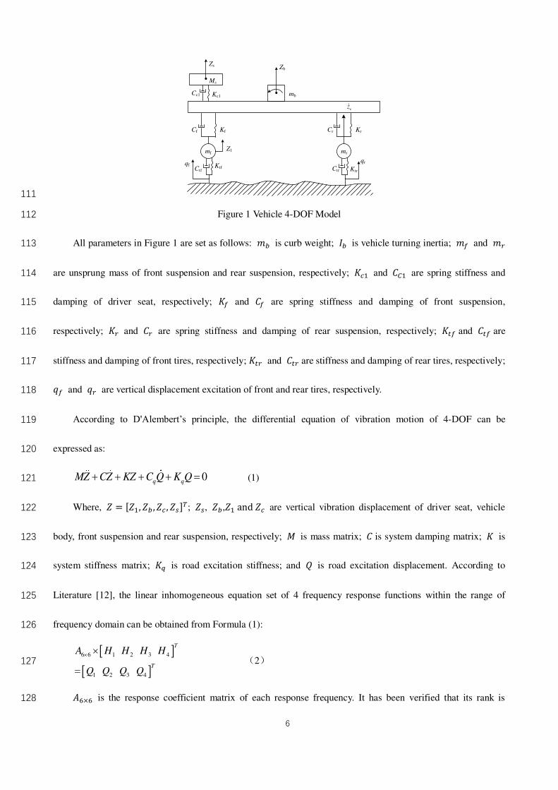
Q t tQQ
Q t tQ
(9) 174
𝑄(𝑡) can be regarded as the generalized single point excitation. Suppose that the auto-spectral density of 𝑄(𝑡) 175
is a known constant, and the exciting moment born by front and rear tires is 𝑡1 and 𝑡2 , respectively, the 176
two-point virtual excitation model obtained with pseudo excitation method can be expressed as: 177
1
2
( ) ( )j t
fj t
qq j tr
qeq S e
qe
(10) 178
Where, �̃�𝑓 and �̃�𝑟 are virtual excitations born by front and rear tires, respectively. 179
3 Vehicle Multi-performance Evaluation Indexes 180
3.1 Evaluation Index of Handling Stability 181
Handling stability of vehicles covers a broad range, which is mainly manifested by the time-frequency 182
response characteristics of vehicles in curve driving. When a vehicle turns a corner at a constant speed, the ratio of 183
yaw velocity to the turning angle of front wheel at a stable state is used as the response evaluation standard. 184
Differently, the value of stable state factor manifests the stable response of vehicles. Generally speaking, the 185
influence of vehicle structure parameters is considered only in the research analysis of stable state response of 186
vehicle when turning a corner. Hence, the influence of dynamic load caused by road random excitation and 187
suspension stiffness and damping and obtaining the improved stability factor was introduced in this paper, so that 188

10
the research of vehicle stability can be more accurate. The improved stability factor 𝐾𝑙(𝑟) in Formula (8) was 189
taken as the evaluation index of listing handling stability here in this paper. 190
3.2 Evaluation Index of Ride Comfort 191
According to GB/T 4970-2009 Test Method of Vehicle Ride Comfort, this paper analyzed the vertical 192
acceleration of the driver’s seat instead of human body acceleration with the weighted acceleration RMS value 193
corresponding to the human body acceleration transferred through seat as the evaluation index of ride comfort. 194
Taking the weighted acceleration RMS value 𝜎𝑧�̈� of the vertical vibration at driver’s seat as the evaluation index 195
of ride comfort, then the formula can be expressed as: 196
22
0( ) ( )
qfzs zs zs qf zW H G f df
(11) 197
Where, 𝑊𝑧𝑠(𝜔) is weighting function (the value is 1 here); 𝐺𝑧𝑞𝑓 (𝜔) is power spectral density inputted by 198
front axle road excitation; 𝐻𝑧𝑠−�̃�𝑓 is vertical acceleration frequency response function of driver’s seat. 199
3.3 Evaluation Index of Economy 200
As the research object, the economy of BEVs is generally evaluated by its power consumption per 100 km at 201
a constant speed. Under the uniform driving condition, the driving force required by the vehicle 𝐹 includes 202
listing resistance 𝐹𝑓 and air resistance𝐹𝑤, i.e., 𝐹 = 𝐹𝑓 + 𝐹𝑤. The power consumption per 100 km of vehicle 203
driving at a constant speed can be calculated with the following formula: 204
22
( ) 21.15 21.15
36( )
D aD a
f W
drive
mc T q mc T q mc T q
C Au C Aumgf S mgfF F SE
(12) 205
Where, 𝑆 = 100𝑘𝑚, 𝑓 is listing resistance coefficient, 𝐶𝐷 is air resistance coefficient, 𝐴 is windward 206
area, 𝑢𝑎 is vehicle driving speed, 𝜂𝑚𝑐 is the efficiency of motor and controller, 𝜂𝑇 is the total efficiency of 207
drive system and 𝜂𝑞 is the average discharging efficiency of accumulator. 208
209

11
4 Mathematical Modeling of Multi-objective Optimization 210
4.1 Mathematical Description of Multi-objective Optimization 211
BEV optimization in this paper means optimizing the parameters of suspension system and battery control 212
strategy on the basis of satisfying all constraints, so as to make the vehicle safe, comfortable and energy-saving 213
under certain conditions and make several target functions in conflict realize the optimal status within a feasible 214
region. Suppose that 𝑋 is the decision space of 𝑛-dimension and 𝑌 is the target space of 𝑛-dimension on the 215
basis of ensuring the loss of generality, then its mathematical modeling of multi-objective optimization can be 216
expressed as [11]
: 217
1 2
1
2
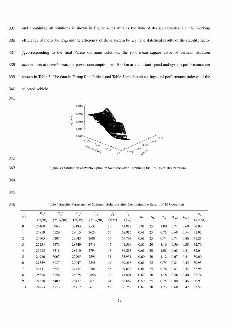
min ( ) ( ) ( ) ( )
. . ( ) 0 ( 1, 2, , )
( ) 0 ( 1, 2, , )
m
i
i
y F x f x f x f x
s t g x i q
h x j q
(13) 218
Where,𝑥 = [𝑥1𝑥2 ⋯ 𝑥𝑛] ∈ 𝑋 ⊂ 𝑅𝑛 is decision vector; 𝑦 = [𝑦1𝑦2 ⋯ 𝑦𝑛] ∈ 𝑌 ⊂ 𝑅𝑚. The objective function 219
𝐹(𝑥) means 𝑚 mapping functions 𝑓: 𝑋 → 𝑌, 𝑔1(𝑥) ≤ 0(𝑖 = 1,2, ⋯ 𝑞1) and ℎ𝑗(𝑥) = 0(𝑗 = 1,2, ⋯ 𝑞2) are the 220
𝑞1 inequation constraints and 𝑞2 equation constraints that the objective function 𝐹(𝑥) needs to satisfy. 221
4.2 Optimization of Objectives 222
The driving conditions set for optimization play a key role, for the speed and road conditions of the vehicle 223
always change in driving. According to the driving conditions set in this paper, the vehicle can be driven stably at 224
a constant speed (30 km/h) along Level B curved road with a 50 m turning radius. Generally speaking, vehicle 225
vibration becomes the most obvious and even resonance may be produced when excitation frequency is 3.15 Hz. 226
In other words, the vehicle's ride comfort and handling stability become the most sensitive. Therefore, the analysis 227
on multi-performance optimization was optimized at a road excitation frequency of 3.15 Hz [12]
. 228
This paper took function 𝑚𝑖𝑛𝜎𝑧�̈� (acceleration RMS value 𝜎𝑧�̈� of the vertical vibration at the driver’s seat), 229
𝑚𝑖𝑛𝐸𝑑𝑖𝑟𝑣𝑒 (power consumption per 100 km at a constant speed) and handling stability factor Kl(r) >0, which mean 230

12
reducing the acceleration RMS value of the vertical vibration at the driver’s seat and power consumption per 100 231
km at a constant speed and making the vehicle lack of turning characteristics properly, as the optimization 232
objectives to meet the requirements of handling stability and ride comfort, and minimize power consumption as 233
much as possible. Set the following functions: 234
1 ( )
2
3
( )
( )
( )
l r
zs
drive
f x K
f x
f x E
(14) 235
Where, 𝑥 is decision variables (or parameters to be optimized), decision variables and corresponding 236
constraint conditions, all of which vary along with specific optimized objects. 237
4.3 Selection of Design Variables 238
The parameters which exert significant influence on the optimization objectives were optimized in this paper. 239
The stiffness of front and rear suspensions and damping of the vehicle are closely related to ride comfort of the 240
vehicle; Meanwhile, vertical load of each vehicle axle changes when the vehicle is listing under the effect of road 241
excitation, moment resulting from sidesway and centripetal force, which means the load that each axle bears has 242
been allocated again in listing, causing the change of cornering stiffness of left and right tires or inside and outside 243
tires, and finally changing the steady state response of the vehicle, as well as the stability factor. Therefore, the 244
stiffness and damping of front and rear suspensions can be regarded as variables of optimization analysis. In 245
consideration of the significant influence of related parameters of BEV’s motor and battery on battery energy 246
consumption, some parameters selected also serve as design variables. All optimized parameters and their 247
selection range are shown in Table 1. 248
Table 1 Parameters to Be Optimized and Constraint Range 249
Type of Parameters Constraint Range
Maxmum power of motor/𝑘𝑤 𝑃𝑒 ∈ [20, 100] Power coefficient of motor 𝑅𝑠 ∈ [0.6, 1.5]

13
Number of battery pack modules/piece 𝑁𝑏 ∈ [20, 30] Axle ratio 𝑅𝑚 ∈ [0.5, 2.5]
Upper limit of battery status/% 𝐻𝑆𝑂𝐶 ∈ [0.55, 0.8] lower limit of battery status/% 𝐿𝑆𝑂𝐶 ∈ [0.2, 0.55] Drive limiting speed/(𝑘𝑤/ℎ) 𝑉𝑒 ∈ [5, 100]
Front suspension stiffness/(𝑁/𝑚) 𝐾𝑓∈ [10475, 37046]
Front suspension damping/(𝑁 ∙ 𝑠/𝑚) 𝐶𝑓 ∈ [2500, 6000] Rear suspension stiffness/(𝑁/𝑚)
𝐾𝑟∈ [16800, 46320] Rear suspension damping/(𝑁 ∙ 𝑠/𝑚) 𝐶𝑟 ∈ [1200, 3600]
Suspension dynamic deflection/(𝑚𝑚) 𝑓𝑑 ∈ [30, 60] 250
4.4 Pareto Optimum Principle 251
Pareto optimum principle serves as a key concept in game theory. Several key concepts are given below 252
based on the symbol definitions in 4.1 [15]
. 253
Definition 1 Pareto dominance. For random vector 𝑢 = [𝑢1𝑢2 ⋯ 𝑢𝑚] ∈ 𝑌, 𝜐 = [𝜐1𝜐2 ⋯ 𝜐𝑚] ∈ 𝑌, if and only if 254
∀𝑖 ∈ {1,2, ⋯ 𝑚}: 𝑢𝑖 ≥ 𝑣𝑖 ∧ ∃𝑗 ∈ {1,2, ⋯ 𝑚}: 𝑢𝑗 > 𝑢𝑗 is true, 𝑣 is superior to 𝑢, or 𝑣 dominates 𝑢, which can be 255
written as 𝑢 ≺ 𝑣. 256
Definition 2 Pareto optimum solution. 𝑥 ∈ 𝑋 is called Pareto optimum solution (or non-dominated solution 257
and non-inferior solution), if and only if 258
→ ∃𝑥′ ∈ 𝑋: 𝐹(𝑥′) = [𝑓1(𝑥′)𝑓2(𝑥′) ⋯ 𝑓𝑚(𝑥′)] ≻ 𝐹(𝑥) = [𝑓1(𝑥)𝑓2(𝑥) ⋯ 𝑓𝑚(𝑥)]. Pareto optimum solution is not 259
dominated by other solutions with the least goal conflict, which can provide decision-makers with a better space 260
for choosing, and can help them make decisions according to the environment or requirements when it is applied 261
to engineering. 262
5 Algorithm Design 263
14
Taking the handling stability factor𝑓1(𝑥) = 𝐾𝑙(𝑟) > 0, acceleration RMS value of vertical vibration at the 264
driver’s seat 𝑓2(𝑥) = 𝑚𝑖𝑛𝜎𝑧�̈� and power consumption per 100 km at a constant speed 𝑓3(𝑥) = 𝑚𝑖𝑛𝐸𝑑𝑖𝑟𝑣𝑒, which 265
mean making the vehicle lack of turning characteristics properly and reducing the acceleration RMS value of the 266
vertical vibration at driver’s seat and power consumption per 100 km at a constant speed as the optimization 267
objectives, this paper proposed the Pareto Optimum Principle-based Multi-Objective Evolutionary Algorithm of 268
EV (EV-MOEA), which is an improvement of non-dominated genetic algorithm (NSGA), with the optimization 269
considering each target equally important and dealing with multi-objective problems, i.e. introducing the elite 270
strategy in the evolutionary process, with the crowding distance and its comparison operator as the basis of the 271
secondary sorting. Finally, the global Pareto optimum solution and the Pareto frontier are obtained. 272
The advantages of EV-MOEA designed in this paper include good exploration performance, used the fast non 273
dominated sorting, reduce the complexity of the non inferior sorting genetic algorithm, with fast non-dominant 274
ranking, complexity of noninferior sorting genetic algorithm, replacing sharing radius with crowding distance and 275
crowding distance comparison operator, as well as fast running speed, which improve the accuracy of the 276
optimization results in a limited way, so that the individuals in the quasi-Pareto domain can extend to the whole 277
Pareto domain and distribute evenly. Introducing the elite strategy maintained the diversity of the population, with 278
good convergence of the solution set, which improved the rapidity and robustness of the optimization algorithm. 279
EV-MOEA has an evolution population, and each candidate solution is expressed by real number encoding. 280
The main procedures of the algorithm are shown in Figure 3. 281

15
282
Figure 3 Flow Chart of EV-MOEA 283
The algorithm is calculated as the steps below: 284
(1) Initialization. Contents in need of initialization mainly include: Scale of evaluation population 𝑁, 285
crossover probability𝑃𝑐 ,, mutation probability𝑃𝑚, maximum generation 𝐺𝑚𝑎𝑥, vehicle model parameters to be 286
optimized, vehicle driving conditions required for simulation, specific performance indexes to be optimized 287
required for the vehicle model, decision space 𝑅𝑚 of m decision variables ( 𝑋1, 𝑋2 , ⋯ 𝑋𝑚 ), i.e. Xi 288
[𝐿𝑖 , 𝐻𝑖](i=1,2,…m) (where, 𝐿𝑖 and 𝐿𝑖 mean lower limit and upper limit of 𝑋𝑖 , respectively). For the engineering 289
application, the precision that can be realized by each parameter of BEV is limited certainly, which is significant 290
only when the value of decision variables is within the range of realizable precision. The significant digit of 291
variables in this paper is set according to precision limitation and maximum generation, with the maximum 292
evolutionary algebra as the condition for judging the completion of evolutionary process. Therefore, the 293
evolutionary algebraic counter 𝐺 needs to be set and initialize into 𝐺 = 0. 294
(2) Evolutionary population generation. The candidate solution is represented by real coding. The process of 295
generating candidate solution gene is as below: First, generate the evaluation 296
population 𝑃𝐺 = {𝑥𝑗 = (𝑥1𝑥2 ⋯ 𝑥𝑖 ⋯ 𝑥𝑚)|𝑥𝑖 ∈ [𝐿𝑖 , 𝐻𝑖], 𝑗 = (1,2, ⋯ 𝑁), 𝑖 = (1,2, ⋯ , 𝑚)} with uniform random 297
number generator, and then truncate the value exceeding the significant digit in 𝑥𝑖 (rounded-off) according to the 298

16
set significant digit. 299
(3) Simulation software calling to initialize the objective function value. Let ∀𝑥𝑗 ∈ 𝑃𝐺 , call 𝑀𝐴𝑇𝐿𝐴𝐵/300
𝑆𝑖𝑚𝑢𝑙𝑖𝑛𝑘 software to test the performance of vehicle model corresponding to 𝑥𝑗 . Simulate the status of the 301
vehicle when driving under specified road conditions and obtain function values of each objective according to the 302
returned results if the performance constraint conditions can be met. To be specific, 𝑓1(𝑥𝑗) is stability factor, 303
𝑓2(𝑥𝑗) is the acceleration RMS value of vertical vibration at driver’s seat and 𝑓3(𝑥𝑗) is the power consumption 304
per 100 km at a constant speed; Otherwise, apply a large enough value to 𝑓1(𝑥𝑗), 𝑓2(𝑥𝑗) and 𝑓3(𝑥𝑗). 305
(4) Calculation of fitness values of candidate solutions. Judge relative advantages and disadvantages of 306
candidate solutions via a specific method. The method applied in the simulation experiments of this paper: First 307
implement non-dominated sorting of 𝑃𝐺 , and then calculate the crowding distance of candidate solutions. 308
(5) Genetic operation to generate new candidate solutions. Select [0.5𝑁] from 𝑃𝐺 with the two-match 309
method, and then carry out SBX and polynomial variation to generate new population 𝑄𝐺. 310
(6) Simulation software calling to calculate the objective function value of descendant candidate solutions. 311
Let ∀𝑥𝑗 ∈ 𝑄𝐺, call 𝑀𝐴𝑇𝐿𝐴𝐵/𝑆𝑖𝑚𝑢𝑙𝑖𝑛𝑘 software to test the performance of vehicle model corresponding to𝑥𝑗 . 312
Simulate the driving status of the vehicle under the specified road conditions and obtain function values of each 313
objective according to the returned results if performance constraint conditions can be met. To be specific, 𝑓1(𝑥𝑗) 314
is stability factor, 𝑓2(𝑥𝑗) is the acceleration RMS value of vertical vibration at driver’s seat, 𝑓3(𝑥𝑗) is the power 315
consumption per 100 km at a constant speed; Otherwise, apply a big enough value to 𝑓1(𝑥𝑗), 𝑓2(𝑥𝑗) and 𝑓3(𝑥𝑗). 316
(7) Evaluation population updating. Obtain new evaluation population with specific strategies. The method 317
applied in the simulation experiments of this paper: First, let 𝑅𝐺 = 𝑄𝐺 ∪, implement non-dominated ranking of 318
𝑃𝐺 and calculate the crowding distance of candidate solutions; then, select 𝑁 candidate solutions from 𝑅𝐺 based 319
on the ranking results to generate new population 𝑃𝐺+1; finally, circulate through 𝐺 = 𝐺 + 1. 320
(8) Output Pareto optimum solution set 𝑃𝐺+1and finish evaluation if the end conditions can be met; 321

17
Otherwise, turn to Step (5). 322
In Step (3) and Step (6), assign a value large enough to𝑓1(𝑥𝑗), 𝑓2(𝑥𝑗) and 𝑓3(𝑥𝑗), respectively, which means 323
that due to its unsuitable handling stability, poor ride comfort and economy, this solution is not directly eliminated 324
for storing diverse genes for subsequent evolutions. 325
326
6 Simulation Verification and Relate Analysis 327
6.1 Experiment Related Settings 328
𝑀𝐴𝑇𝐿𝐴𝐵/𝑀 − 𝐹𝑖𝑙𝑒 was used to program realization for EV-MOEA, with the scale of evaluation population 329
as 32, maximum generation as 100, mutation probability as 0.1 and crossover probability as 0.9. The basic 330
parameter configuration of simulated the whole vehicle is shown in Table 3. 331
Table 3 Basic Parameters of the Vehicle 332
Item Parameter Value
Drive the Motor
Maxmum
power/kW 75
Maxmum output
torque/(𝑁 ∙ 𝑚) 275
Maxmum
speed/(𝑟 ∙𝑚𝑖𝑛−1)
10 000
Accumulator
Type
Qty./pcs 25
Single module
index 12𝑉, 25𝐴 ∙ ℎ
Parameters of the
Vehicle
Total weight of
vehicle (kg) 1350
Windward area
(m2) 1.9
Air resistance
coefficient 0.335
6.2 Optimization Results and Analysis 333
The distribution of the final Pareto optimum solutions after making statistics on the results of 10 operations 334
18
and combining all solutions is shown in Figure 4, as well as the data of design variables. Let the working 335
efficiency of motor be 𝐸𝑀𝐶and the efficiency of drive system be 𝐸𝐺 . The statistical results of the stability factor 336
𝑓1 corresponding to the final Pareto optimum solutions, the root mean square value of vertical vibration 337
acceleration at driver's seat, the power consumption per 100 km at a constant speed and system performance are 338
shown in Table 5. The data in Group 0 in Table 4 and Table 5 are default settings and performance indexes of the 339
selected vehicle. 340
341
0.0032
0.0029
0.0026
0.0023
0.0020
0.074
0.089
0.122
0.146
0.17
f 1(s
2/m
2)
342
Figure 4 Distribution of Pareto Optimum Solutions after Combining the Results of 10 Operations 343
344
345
Table 4 Specific Parameters of Optimum Solutions after Combining the Results of 10 Operations 346
No. 𝐾𝑓/ (𝑁/𝑚)
𝐶𝑓/ (𝑁 ∙ 𝑆/𝑚)
𝐾𝑟/ (𝑁/𝑚)
𝐶𝑟/ (𝑁 ∙ 𝑆/𝑚)
𝑓𝑑 (𝑚𝑚)
𝑃𝑒 (𝑘𝑤) 𝑅𝑆 𝑁𝑏 𝑅𝑚 𝐻𝑠𝑜𝑐 𝐿𝑠𝑜𝑐
𝑣𝑒 (𝑘𝑚/ℎ)
0 26460 5063 37183 2532 50 41.017 1.01 25 1.00 0.71 0.60 30.00
1 24819 5129 29015 2624 55 68.916 0.61 25 0.75 0.68 0.54 31.02
2 24905 5207 29643 2601 53 69.703 0.61 25 0.74 0.71 0.46 31.21
3 25134 5473 28349 2718 47 41.569 0.65 20 1.16 0.56 0.38 32.70
4 25685 5318 28710 2794 43 36.213 0.61 20 1.08 0.68 0.41 32.64
5 24986 5067 27965 2591 51 35.951 0.60 20 1.12 0.67 0.41 30.69
6 27359 6137 29047 2548 49 69.218 0.61 25 0.75 0.81 0.45 30.95
7 26741 6243 27934 2501 45 69.026 0.61 25 0.76 0.81 0.44 32.95
8 25834 6154 26075 2856 39 41.001 0.67 20 1.18 0.56 0.40 32.74
9 24378 5409 28437 2673 41 68.667 0.59 25 0.75 0.80 0.45 30.93
10 24953 5173 25712 2613 57 36.759 0.62 20 1.23 0.68 0.42 32.52

19
Table 5 System Performance Corresponding to Pareto Optimum Solutions after Combining the Results of 10 Operations 347
No.
Objective Function Value System Performance 𝑓1/ (𝑠2/𝑚2)
𝑓2/ (𝑚/𝑠2)
𝑓3 (𝑘𝑤 ∙ ℎ/100𝑘𝑚) 𝐸𝑀𝐶 𝐸𝐺
0 0.0023 0.114 15.89 0.79 0.89
1 0.0026 0.101 13.73 0.91 0.91
2 0.0027 0.112 13.95 0.89 0.93
3 0.0029 0.109 13.96 0.75
0.86
0.94
4 0.0025 0.112 14.25 0.93
5 0.0023 0.111 14.37 0.85 0.92
6 0.0021 0.110 13.98 0.89 0.91
7 0.0029 0.109 13.29 0.71 0.92
8 0.0023 0.106 13.17 0.88 0.94
9 0.0024 0.108 14.56 0.85 0.93
10 0.0025 0.104 14.59 0.79 0.91
It can be found from the data in Table 5 that the optimized system has reduced the acceleration RMS value of 348
vertical vibration at driver’s seat and the power consumption per 100 km at a constant speed under the premise of 349
guaranteeing vehicle handling stability. In the optimized system, stability factors have increased by 9.5%, the 350
acceleration RMS value of vertical vibration at driver’s seat has decreased by 5.1% and the power consumption 351
per 100 km at a constant speed has decreased by 8.8% on average, respectively. 352
As for the efficiency of the system, the efficiency of motor and driving system has increased by 6.1% and 3.8% 353
on average, respectively, which implies that the working efficiency of major components of the vehicle has 354
increased after optimization and each subsystem has better matched, so the multi-performance optimization 355
proposed in this paper can improve the total working efficiency of BEVs. 356
As an example, the optimization solution of Group 1 was compared with the system before optimization. 357
Figure 5 and Figure 6 show the comparison results of the efficiency of motor and driving system, respectively. 358

20
359
(a) Before optimization (b) After optimization 360
Figure 5 Comparison Figure on Working Efficiency of Motor 361
According to Figure 5, the efficiency of motor was mainly within [0.7, 0.95] before optimization but within 362
[0.8, 0.95] after optimization, while the working points of optimized motor were highly distributed in the high 363
efficient areas after comparing the distribution diagram on working points of motor, which indicates that the 364
efficiency of optimized motor has been significantly improved, which is further helpful to improve the economy 365
of BEVs. 366
367
368
(a) Before optimization (b)After optimization 369
Figure 6 Efficiency Comparison of Driving System 370
371
According to Figure 6, the efficiency of driving system was within [0.8, 0.9] approximately before 372
optimization but mainly within [0.85, 0.95] after optimization, which shows that the efficiency of driving system 373
after optimization is superior to that before optimization, which is helpful to improve the comprehensive 374
efficiency of BEVs. 375

21
7 Conclusions 376
To address the multi-performance optimization of BEVs, this paper proposed the corresponding model and 377
algotithm for the multi-objective evaluation based on Pareto optimum principle with handling stability, ride 378
comfort and economy as optimization objectives and improved ride comfort and economy under the premise of 379
guaranteeing vehicle handling stability. The effectiveness of the method has been verified through simulation test 380
and the following conclusions have been made. 381
(1) Multi-objective optimization algorithm of BEVs proposed based on Pareto optimum principle can 382
improve ride comfort of vehicles and reduce energy consumption of batteries under the premise of guaranteeing 383
handling stability. According to the simulation experiment, the algorithm has optimized multi-performance target 384
collaboratively such as the safety, comfort and energy conservation of BEVs. 385
(2) The working efficiency of motor and driving system of BEVs have been improved differently after 386
optimization, which means that each subsystem has been better matched after optimization and BEVs show a 387
better performance. 388
(3) The method proposed in this paper makes it unnecessary to simplify the multi optimization objectives 389
into one, which avoids the adverse influence caused by the weighted sum of different objectives, providing many 390
groups of optimum solutions. 391
392
Availability of data and materials 393
All data generated or analysed during this study are included in this published article [and its supplementary 394
information files]. 395
Acknowledgments 396
We hereby would like to extend our gratitude towards the sponsors that supported this study, the National 397

22
Key Research and Development Plan (Grant No.: 2016YFB0100900). 398
Authors’ Contributions 399
Yawei Chen and Qian Cheng wrote the manuscript; Jurui Liu was in charge of the whole trial, review and 400
edition; Xixiang Hao and Chenheng Yuan assisted with review. All authors read and approved the final 401
manuscript. 402
Authors’ Information 403
Yawei Chen was born in Dingxi, Gansu, China, in 1993. He received the M.S. in Vehicle engineering in 2019 404
from Chongqing Jiaotong University. He is currently a vehicle Engineer at the China Automotive Engineering 405
Research Institute. His current research interests include electric vehicle and dynamics. 406
Qian Cheng was born in Chongqing, China, in 1993. He received the B.S. degree in automobile support 407
engineering in 2016, the M.S. degree in vehicle operation engineering in 2019 from Chongqing Jiaotong 408
University. He is currently a vehicle Engineer at the China Automotive Engineering Research Institute. His current 409
research interests include electric vehicle and dynamics. 410
Jurui Liu was born in Changchun, Jilin, China, in 1988. She received the M.S. in HVAC engineering from 411
the Jilin Jianzhu University, Jilin, China, in 2019.She currently works in Beijing Yunshan World Information 412
Technology company. Her current work includes automatic control, big data and machine learning. 413
Xixiang Hao was born in Anqing, Anhui, China, in 1991. He received the M.S. in Traffic and transportation 414
from Chongqing Jiaotong University, Chongqing, China, in 2019.He currently works in Zhejiang Sanhua 415
Automotive components Co. LTD. His current research interests include Intelligent control and Thermal 416
management of equipment. 417
Chenheng Yuan was born in Xichong, Sichuan, China, in 1984. He received the Ph.D. degrees in power 418
machinery and engineering from the Beijing Institute of Technology, Beijing, China, in 2015. From 2016 to 2019, 419
He was an Associate Professor with Automobile Application Engineering Department, Chongqing Jitaotong 420

23
University. Since 2019, he has been a Professor with the School of Traffic and Transportation, Chongqing 421
Jiaotong University. His current research interests include electric vehicle, hybrid electric system and electronic 422
control. 423
Funding 424
Supposed by the National Key Research and Development Plan (Grant No.: 2016YFB0100900). 425
Competing Interests 426
The authors declare no competing financial interests. 427
Author Detail 428
1China Automotive Engineering Research Institute Co., Ltd. , Chongqing 401147, China.
2Beijing Yunshan 429
World Information Technology Co., Ltd., Beijing 100006, China. 3Zhejiang Sanhua Auto Parts Co., Ltd., 430
Hangzhou, Zhejiang 311200, China. 4Chongqing Jiaotong University College of Traffic & Transportation, 431
Chongqing 400074, China. 432
References 433
[1] ELS P S, UYS P E. Investigation of the applicability of the dynamic-Q optimization algorithm to vehicle suspension design[J]. 434
Mathematical & Computer Modeling, 2003, 37( 9 /10) :1029-1046. 435
[2] GONCALVES J P C, AMBRSIO J A C. Optimization of vehicle suspension systems for improved comfort of road vehicles 436
using flexible multi-body dynamics [J]. Nonlinear Dynamics, 2003, 34( 1) : 113-131. 437
[3] YANG Y, REN W, CHEN L, et al. Study on ride comfort of tractor with tandem suspension based on multi-body system 438
dynamics [J]. Applied Mathematical Modelling, 2009, 33(1) : 11-33. 439
[4] YANG Rongshan, YUAN Zhongrong, HUANG Xiangdong, et al. Research on the Collaborative Optimization of Vehicle 440
Handling Stability and Ride Comfort [J]. Automotive Engineering, 2009, 31 (11): 1053-1059. 441
[5] XU Haijiao. Analysis of Vehicle Handling Stability and its Multi-objective Optimization Design [D]. Handan: Hebei University 442
of Engineering, 2015, 51-62. 443

24
[6] SONG Kang, CHEN Xiaokai, LIN Yi. Multi-objective Optimization of Vehicle Driving Dynamics Performance [J]. Journal of 444
Jilin University (engineering science edition) 2015, 45 (2): 352-357. 445
[7] CHEN Yikai, HE Jie, ZHANG Weihua et al. Improvement of Ceiling Control Strategy for the Suspension System of Multi-axle 446
Heavy Truck [J]. Journal of Agricultural Machinery, 2011, 42 (6): 16-22. 447
[8] ZHENG Zhifei, LIU Jianli, XU Zhongming, YANG Jianguo et al. Optimization of Commercial Vehicle Suspension Parameters 448
for Smoothness and Road Friendliness [J]. Automotive Engineering, 2014, 36 (7): 889-893. 449
[9] YANG Kun. Simulation and Multi-objective Optimization of Smoothness and Road Friendliness of Six-axle Semi-trailer Train 450
[D]. Changchun: Jilin University, 2017, 58-75. 451
[10] ZHOU Feikun. Research on Dynamic System Parameter Matching and Vehicle Control Strategy of Battery Electric Vehicles 452
[D].Changchun: Jilin University, 2013. 453
[11] ZHANG Kangkang. Research on the Efficiency Optimization Method of Battery Electric Vehicles [D]. Beijing: Tsinghua 454
University, 2014. 455
[12] LIN Jiahao, ZHANG Yahui. Virtual Excitation Method for Random Vibration [M]. Beijing: Science Press, 2004:42-57. 456
[13] YU Zhisheng. Automobile Theory [M]. Beijing: Machinery Industry Press, 2009. 457
[14] ZHANG Jingmei. Research on Dynamic Performance and Multi-objective Optimization of Heavy-duty Vehicles [D]. Beijing: 458
Beijing Jiaotong University, 2018. 459
[15] YGANG Guansi, LI Shaobo, QU Jinglei et al. Multi-objective Optimization of Hybrid Vehicle Based on Pareto Optimal 460
Principle [J]. Journal of Shanghai Jiaotong University, 2012, 46 (8): 1297-1309. 461
Related Documents