Collaborative penalized Gaussian mixture PHD tracker for close target tracking

Collaborative Penalized Gaussian mixture PHD tracker

for close target tracking

Yan Wanga,b, Huadong Menga, Hao Zhanga, Xiqin Wanga

aISL Laboratory, Department of Electronic Engineering, Tsinghua University, Beijing,

ChinabRadar Institute, EAAF, Beijing, China

Abstract

The Gaussian Mixture Probability Hypothesis Density (GM-PHD) recursionis a promising computationally tractable implementation for the ProbabilityHypothesis Density (PHD) filter. The competitive GM-PHD (CGM-PHD)and penalized GM-PHD (PGM-PHD) filter employ renormalisation schemesto refine the weights assigned to each target and improve the estimationperformance of GM-PHD filter for closely spaced targets to some extent.However both methods do not provide target trajectories in time and theproblem of wrongly identifying close targets for GM-PHD tracker is not stillsolved well. In this paper we propose a collaborative penalized scheme toimprove the drawback of GM-PHD tracker by utilizing the track label ofeach Gaussian component in GM-PHD recursion. The simulation resultsshow that the collaborative penalized GM-PHD (CPGM-PHD) tracker notonly can improve the estimation accuracy of target number and states butalso provide the right identities of targets in close proximity.

Keywords:

closely spaced targets, Probability Hypothesis Density (PHD), CompetitiveGM-PHD, Penalized GM-PHD

1. Introduction

Multi-target tracking (MTT) aims at jointly estimating an unknown num-ber of targets as well as their states to obtain target trajectories from seriesof noisy measurements in the presence of spurious targets (clutter) and un-certainty in detection. The traditional methods based on data association

Preprint submitted to Signal Processing June 24, 2013

such as Global Nearest Neighbor (GNN), Joint Probabilistic Data Associa-tion (JPDA) [1–4] and Multiple Hypotheses Tracking (MHT) [1, 2, 5] all mapthe multi-target tracking into independently tracking of each single target byassociating one measurement with one existing track at each time step.

Using Random finite set (RFS) [6, 7] to model the collections of targetsand measurements as a whole respectively, the finite set statistics theory(FISST) provides a rigorous Bayesian framework for MTT, and avoids theexplicit associations between measurements and targets at the step of stateestimation. The PHD filter [8, 9] proposed by Mahler and realized by Voetc. propagates the first-order statistical moment or intensity of the stateRFS in time and is an effective approximation of the multi-target Bayesianposterior. There are two major implementations of the PHD filter known asparticle-PHD filter or SMC-PHD filter [10–12] and GM-PHD filter [13]. Thelatter propagates a sum of weighted Gaussian components representing thePHD function for linear Gaussian models.

In order to obtain target trajectories, generally it is necessary to reprocessidentity-free estimates provided by the GM-PHD filter or the SMC-PHDfilter. Some novel data association schemes for the SMC-PHD filter [14–16]are proposed to associate the target state estimates by reference to traditionalassociation approaches such as MHT. The GM-PHD tracker [17] determinesthe target trajectories directly from the evolution of the Gaussian mixture,within which each single Gaussian demonstrates each possible trajectory [17–19].

When targets are coming near each other, such as small angle crossing orocclusion condition, the performance of the original GM-PHD filter dramati-cally decreases. It is difficult to resolve identities of targets in close proximityfor GM-PHD tracker on its own [17–20], or leads to missing the estimates ofthe close targets [21–24]. The competitive GM-PHD (CGM-PHD) filter andpenalized GM-PHD (PGM-PHD) are proposed in the latest papers [22, 23]and both employ renormalization schemes to re-manage the weights assignedto each target. When targets are coming near to each other, the filters se-lect the optimal measurement for each predicted target one by one throughrearranging weights, which effectively improves the drawback of likely miss-ing closely spaced targets for GM-PHD filter. However, both filters do notprovide the continuous trajectories of targets. The problem of likely wronglyidentifying close targets for GM-PHD tracker is not still solved well. For theCGM-PHD tracker and PGM-PHD tracker implemented by arranging labelsto Gaussian mixture like GM-PHD tracker it is still difficult to distinguish

2

between close targets in respectable scenarios. One possible outcome wouldbe the assignment of the same identity to multiple target tracks, and anotheris that identities are wrongly assigned to closely spaced targets.

In MTT problem there is such a one-to-one assumption that at eachtime step one measurement is generated from only one target and one targetcan only generate one measurement. In the association step of MHT in apossible joint event of hypothesis trajectories each trajectory is associatedwith an unique measurement series over time. The CGM-PHD tracker andPGM-PHD tracker only consider the one-to-one association between eachmeasurement at current time step and each possible trajectory, but ignore theuniqueness of the history measurement series associated by each trajectory.So different measurements are possibly assigned to different trajectories butwith same identity for CGM-PHD or PGM-PHD, and finally the targets arewrongly identified.

Considering that there is a one-to-one correspondence between each mea-surement and each target with different identity, in this paper we propose anovel scheme of the weight rearrangement called collaborative penalized GM-PHD (CPGM-PHD) and utilize the track label of each Gaussian componentin GM-PHD recursion to collaboratively penalize the weights of targets withthe same identity. Besides, to avoid enlarging spurious targets by weightrearrangement we propose to just process the steady trajectories and keepthe weights of those temporary targets unchanged. The scheme effectivelyreduces spurious trajectories generated by improper weight rearrangement inthe CGM-PHD tracker and PGM-PHD tracker.

The performance of the proposed CPGM-PHD tracker is compared withthe original GM-PHD tracker, CGM-PHD tracker and PGM-PHD tracker ina number of experiments by simulating closely spaced targets with variousuncertainties in noise, clutter rate and probability of detection. The sim-ulation results show that our method not only can improve the estimationaccuracy of target number and states but also more accurately provide theidentities of targets when they are coming near each other.

The rest of the paper is organized as follows. Section 2 reviews thePHD filter and the GM-PHD tracker. Section 2 also analyzes the prob-lem of wrongly identifying close targets with the existing GM-PHD-basedapproaches. The proposed CPGM-PHD tracker is explained in Section 3.For illustration purposes, simulation results for our proposed method aregiven in Section 4. Finally, concluding remarks and possible future researchdirections are given in Section 5.

3

2. Problem formulation

2.1. Multi-target RFS modeling and PHD filter

In a multi-target system, considering plenty of uncertainty in target statesand numbers such as that targets appear, dynamically move, split and dis-appear, multi-target states and measurements constitute RFSs. The RFSsof the multi-target states and measurements at time step k are modeled asXk = {xk,1, . . . , xk,M(k)} and Zk = {zk,1, . . . , zk,N(k)}, respectively. Then, theMTT problem can be posed as a filtering problem in RFS state space andmeasurement space.

The PHD filter is an approximation to the multi-target Bayes filter, whichmakes the recursion computationally tractable. From the PHD function ofthe multi-target state RFS the local maxima can be used to generate thestate estimates of targets.

The PHD recursion is as follows,

Dk/k−1(x) =

∫

pS,k(ζ)fk/k−1(x|ζ)Dk−1(ζ)dζ

+

∫

βk/k−1(x|ζ)Dk−1(ζ)dζ + γk(x),

(1)

Dk(x) =[1− pD,k(x)]Dk/k−1(x)

+∑

z∈Zk

pD,k(x)gk(z|x)Dk/k−1(x)

κk(z) +∫

pD,k(ζ)gk(z|ζ)Dk/k−1(ζ)dζ,

(2)

where γk(x) denotes the intensity of spontaneous target birth; fk/k−1(.|.) isthe probability density of Markov transition between target states; βk/k−1(.|.)denotes the intensity of spawned target; gk(.|.) is the likelihood function ofmeasurement to state; κk(z) is the intensity of the clutter RFS and equalsλkck(z), where λk is the mean number of clutter points in compliance withPoisson distribution; pS,k is the survival probability of targets and pD,k is thedetection probability.

For linear Gaussian models there is a closed-form solution for PHD filter,called GM-PHD filter.

2.2. GM-PHD filter and labeling

Assuming that the Markov dynamic model to which targets move accord-ing and the measurement model are both linear Gaussian, i.e.,

fk/k−1(x|ζ) = N(x;Fk−1ζ, Qk−1), (3)

4

gk(z|x) = N(z;Hkx,Rk), (4)

where N(x;m,S) denotes a Gaussian density with mean m and covarianceS. The parameter Fk−1 is the state transition matrix, Qk−1 is the processnoise covariance, Hk is the observation matrix and Rk is the observation noisecovariance.

Assuming that the intensities of the birth and spawn RFSs are bothGaussian mixtures, and the posterior intensity at time step k−1 is a Gaussianmixture, then, the predicted and updated PHD are also Gaussian mixturesas follows,

Dk/k−1(x) =

Jk/k−1∑

j=1

wjk/k−1N(x;mj

k/k−1, Pjk/k−1), (5)

Dk(x) =[1− pD,k(x)]Dk/k−1(x)

+∑

z∈Zk

Jk/k−1∑

j=1

wjk(z)N(x;mj

k/k(z), Pjk/k).

(6)

where Jk/k−1 is the number of predicted Gaussian components, wjk/k−1,m

jk/k−1

and P jk/k−1 are respectively the weight, mean and covariance of the j-th pre-

dicted component, and mjk/k(z), P

jk/k are respectively the mean and covari-

ance of the updated component by measurement z to the j-th predictedcomponent.

The GM-PHD tracker records the evolution of each Gaussian component.Assuming Jk−1 is the number of Gaussian components at time step k − 1,in the prediction process the same labels with the existing Jk−1 Gaussiancomponents are assigned to the corresponding predicted Jk−1 componentsand other spawn or birth components are newly labeled. According to (6),Jk/k−1 predicted Gaussian components are kept in [1 − pD,k(x)]Dk/k−1(x),and each measurement z ∈ Zk is used to update all the Jk/k−1 predictedGaussian components. Each predicted component gives rise to 1+ |Zk| Gaus-sian components with the same identity label, where |Zk| is the number ofmeasurements. As a result, a number of updated Gaussian components forevery predicted Gaussian component constructs a part of tree structure. Allbranches of a tree have the same identity label and each branch is a possibletrajectory of a target. The GM-PHD tracker is to select the branch with thelargest weight as the individual target track from each tree demonstratingall possible tracks of each target.

5

−10 −5 0 5 100

0.05

0.1

0.15

0.2

x (m)

PH

D (

k−1/

k−2)

A predictionB prediction

z1k−1

: x=6.6

z2k−1

: x=2

−10 −5 0 5 100

0.05

0.1

0.15

0.2

x (m)

PH

D (

k−1)

A1: A updated by z1k−1

A2: A updated by z2k−1

B1: B updated by z2k−1

−10 −5 0 5 100

0.05

0.1

0.15

0.2

x (m)

PH

D (

k/k−

1)

A1 predictionA2 predictionB1 prediction

z1k: x=1.5

z2k: x=2.5

−10 −5 0 5 100

0.05

0.1

0.15

0.2

x (m)

PH

D (

k)

A11: A1 updated by z1k

A12: A1 updated by z2k

A21: A2 updated by z2k

B11: B1 updated by z2k

(3)

(2)

(4)

(1)

wBk−1/k−2

N(z1k−1

;zBk−1/k−2

,Pk−1/k−2

)

wA1k/k−1

N(z2k;zA1

k/k−1,P

k/k−1)

Figure 1: An ambiguity example of tracking two close targets for GM-PHD filter.

In order to reduce the computational load, pruning the Gaussian com-ponents with low weights and merging the Gaussian components within acertain distance are necessary.

2.3. Drawback of the existing GM-PHD-based approaches

Ideally, in each tree structure representing each target one rather largebranch can be picked as an estimation. However, when targets come neareach other, the situation is not so ideal. If the distances of more than onemeasurement towards one trajectory or multiple possible trajectories of onetarget are smaller than that towards other targets, more than one branch ofan individual target would be reported as the estimated targets and someother target would be missed at that time. For this reason, the performancesof the existing GM-PHD-based approaches decrease in tracking closely spacedtargets.

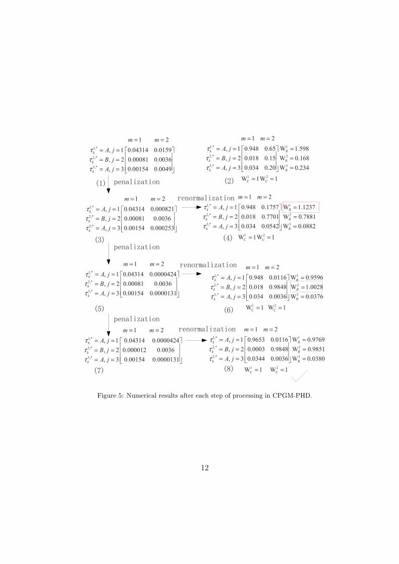
We take an example of tracking two closely spaced targets as shown in Fig.1. Regardless of merging, we show individually each Gaussian demonstratingeach possible trajectory and multiple Gaussians in the Gaussian mixture arenot added up.

Suppose that there is no clutter and all the measurements generated bytargets are detected. Two close targets are with the identity A and B, re-spectively. Fig. 1 (1) shows the measurements at time step k−1 and the pre-dictions of target A and B. Due to that wB

k−1/k−2N(z1k−1; zBk−1/k−2, Pk−1/k−2)

is very small where zBk−1/k−2 is the predicted measurement of target B, there

6

are only three updated components, respectively as shown as the curves A1,A2 and B1. Supposing that the means of A1, B1 and A2 are respectivelyx1k−1, x

2k−1, x

3k−1, the estimations x1

k−1 and x2k−1 with weights w > 0.5 are

outputted. As shown in Fig. 1 (3) due to that wA1k/k−1N(z2k ; z

A1k/k−1, Pk/k−1) is

more than that of z2k towards other predicted measurements and z1k is moreclose to the prediction of A1 than other predictions, we get the four largeupdated Gaussian components as shown in Fig. 1 (4). There are two ratherlarge branches of target A with weights w > 0.5, and target B has onlylarge branch but with weights far less than 0.5 as shown as the curve B11.Considering the Gaussian components within a certain distance would bemerged, the Gaussians A21 and B11 would be merged into one with the onlyidentity A for the weight of A21 is bigger than that of B11. Then, the targetB is missing. Regardless of merging, the means of A11 and A12 are reportedas estimations. Let xn,m be the Gaussian mean by updating the predictionxnk/k−1 with the measurement zm, then the means of A11 and A12, x1,1 and

x1,2, respectively, are reported.

1,1 0.948w =

1,2 0.65w =

3,1 0.034w =

3,2 0.2w =

2,2 0.15w =

2,1 0.018w =

BA

(a) Tree structure of GM-PHD

BA

(b) Change of the tree structures forPGM-PHD

Figure 2: The tree structures of tracking two targets in the example given in Fig. 1.

Assuming the weight of the branch xn,m is wn,m, Fig. 2a shows the treestructures of two targets in the example given in Fig. 1. The branches with

7

BA BA

Figure 3: Change of the tree structures of tracking two targets in the example given inFig. 1 by weight rearrangement of our proposed method.

the same color are generated at the same time step, and the height of thebranch is equivalent to the weight of the branch.

We briefly illustrate the principle of PGM-PHD and CGM-PHD usingFig. 2b. After selecting the tallest branch (with the largest weight) of sometree, the other branches at the same node of the tree are cutted short tomake the branches of other trees grow by renormalization of weights. Af-ter rearrangement by PGM-PHD the new tree structures of two targets areshown in Fig. 2b and the result of CGM-PHD is similar. The weaker tree Bfinally has a rather tall branch by the rearrangement.

However, due to that just the branches at the same node with the tallestbranch in the tree A are cutted short, not only the branches of the treeB grow but also the branches from other nodes in the tree A grow rapidlyas shown in Fig. 2b. For the branch x3,2 in the tree A is also large andeven taller than the biggest branch x2,2 in the tree B, the weaker tree B isstill blocked and gradually withers down during a period of time. So, forPGM-PHD tracker and CGM-PHD tracker one possible outcome would bethe assignment of the same identity to multiple target trajectories and thetrue identity of some target perhaps is missing. Besides, weeds (spurioustarget) near the two trees perhaps grow.

Our goal is to make both trees representing two targets thrive as far aspossible. Considering that there is a one-to-one correspondence between eachmeasurement and each target with different identity, that is, some unique

8

branch in each tree, we propose to cut short all the other branches in thetallest tree with keeping the tallest branch so as to make the other tree nearbygrow better. The ideal result is shown as Fig. 3. Our proposed method iscalled collaborative penalized GM-PHD tracker.

3. Collaborative penalized GM-PHD Tracker

This section explains the specific scheme of collaborative penalized GM-PHD (CPGM-PHD) tracker.

Let wj,mk and wj,m

k be the weight and the normalized weight of the targetxj,mk respectively,

wj,mk = pD,kw

jk/k−1N(zmk ;Hkm

jk/k−1, Rk +HkP

jk/k−1(Hk)

T ), (7)

wj,mk =

wj,mk

κk(zmk ) +∑Jk/k−1

i=1 wi,mk

, (8)

where zmk is the m-th measurement at time step k. The parameters Rk andHk are defined in (4), κk(.) in (2).

All the unnormalized weights of all predicted targets constitute a Jk/k−1×Mk-order weight matrix Mw, and the normalized weights construct anotherweight matrix Mw, where Mk is the number of measurements at time stepk and Jk/k−1 is the number of Gaussian predicted components. The element

< j,m > is the weight of the Gaussian{

mj,mk , P j,m

k

}

corresponding to the

target xj,mk which is created by updating the predicted target xj

k/k−1 using

the measurement zmk . Each predicted target has an identity label τ jk/k−1,and all the Gaussians generated by the same predicted target and differentmeasurements have the same label, that is, τ j,mk = τ jk/k−1. Each Gaussian in

the Gaussian mixture consists of four parts{

wj,mk , mj,m

k , P j,mk , τ j,mk

}

.When targets are coming near each other, for more than one measurement

is closer to one target compared to the other targets multiple Gaussians inthe same row of the normalized matrix Mw have enough large weights so asthat the total weight

∑Mk

m=1 wj,mk is greater than one. When

∑Mk

m=1wj,m

k > 1 (9)

the j-th target is called an inconsistent target.

9

Then, in order to improve the drawback mentioned above, we propose toselect the optimal association pair < j∗, m∗ > between target xj∗

k/k−1 and all

the measurements according to the normalized matrix Mw, and penalize allthe other Gaussians with the same label as τ j

∗,m∗

k by decreasing their weightsin the unnormalized weight matrix Mw. Then, the weights in each columnof new Mw are renormalized to construct a new normalized matrix.

Firstly, the target with the greatest weight in the normalized matrix Mw

is found as< j∗, m∗ >= argmax

j∈I and ∀m=1:Mk

(wj,mk ), (10)

where I = {1, ..., Jk/k−1}.In the algorithm of the original CGM-PHD filter or PGM-PHD filter

once the total weight of the remaining target with maximum weight is lessthan one, the rearrangement processing is terminated, which is sometimesimproper. Often the target with the largest weight meets the condition oftarget consistency and perhaps other targets are still inconsistent as (9). Sowe choose to check one by one whether each target is inconsistent until thetotal weight of each target in the remaining rows is less than one. In order toreduce the computational load, we can also set an end criterion, such as thatthe remaining maximum weight is less than a given threshold, for instance,0.3. If the remaining maximum weight wj∗,m∗

k is less than the given threshold,we have reason to believe that the total weight of the row is less than one.Even if this is not the case, the change by weight rearrangement would beslight for that the penalization factor (1− wj∗,m∗

k ) is fairly large.

So, if the total weight∑Mk

m=1 wj∗,mk is less than one, ignore the j∗ row and

select the target with the greatest weight in the remaining rows until that thetotal weight

∑Mk

m=1 wj,mk is greater than one. If wj∗,m∗

k is the greatest weight,we penalize the other components except the element < j∗, m∗ > in the j∗

row of the unnormalized weight matrix Mw and all the components in otherrows with the same label as τ j

∗,m∗

k . The new unnormalized weight matrixMnew

w is calculated as

wj,mk,new =

wj,mk , m = m∗

wj,mk × (1− wj∗,m∗

k ), j = j∗, ∀m = 1 : Mk, m 6= m∗

wj,mk × (1− wj∗,m∗

k ), j 6= j∗, τ j,mk = τ j∗,m∗

k , ∀m = 1 : Mk, m 6= m∗

wj,mk j 6= j∗, τ j,mk 6= τ j

∗,m∗

k , ∀m = 1 : Mk, m 6= m∗.(11)

10

1 1,1,* 1,1 1,2

2,* 2,1 2,2 2 2,

3,* 3,1 3,2 3 3,

1 ,1 2 ,2

1 2

W, 1

, 2 W

, 3 W

W W

m

R mk

m

k R m

mk R m

j j

C Cj j

m m

wA j w w

B j w w w

A j w w w

w w

τ

τ

τ

= =

= != =

" #= = =" #

" #= = =$ %

= =

&&&

& &

1,* 1

2,* 2

3,* 3

1 2

1 2

, 1 0.948 0.088 W 1.036

, 2 0.018 0.386 W 0.404

, 3 0.034 0.526 W 0.560

W 1W 1

k R

k R

k R

C C

m m

A j

B j

A j

τ

τ

τ

= =

= = = !" #

= = =" #" #= = =$ %

= =

1,* 1

2,* 2

3,* 3

1 2

1 2

, 1 0.948 0.052 W 1

, 2 0.018 0.406 W 0.424

, 3 0.034 0.542 W 0.576

W 1W 1

k R

k R

k R

C C

m m

A j

B j

A j

τ

τ

τ

= =

= = = !" #

= = =" #" #= = =$ %

= =

1,* 1

2,* 2

3,* 3

1 2

1 2

, 1 0.948 0.65 W 1.598

, 2 0.018 0.15 W 0.168

, 3 0.034 0.20 W 0.234

W 1W 1

k R

k R

k R

C C

m m

A j

B j

A j

τ

τ

τ

= =

= = = !" #

= = =" #" #= = =$ %

= =

1,*

2,*

3,*

1 2

, 1 0.04314 0.0159

, 2 0.00081 0.0036

, 3 0.00154 0.0049

k

k

k

m m

A j

B j

A j

τ

τ

τ

= =

= = !" #

= = " #" #= = $ %

1,* 1,1 1,2

2,* 2,1 2,2

3,* 3,1 3,2

1 2

, 1

, 2

, 3

k

k

k

m m

A j w w

B j w w

A j w w

τ

τ

τ

= =

!= =

" #= = " #

" #= = $ %

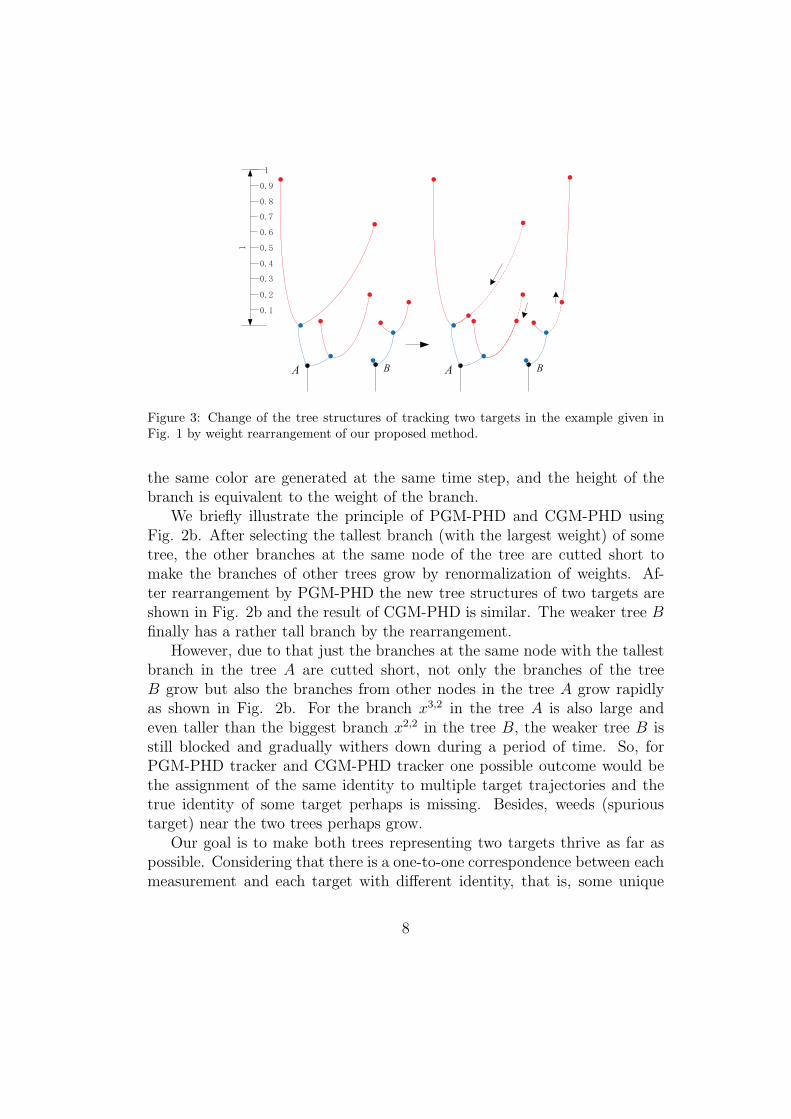
Figure 4: Result of rearrangement by PGM-PHD and CGM-PHD. (1) Symbolic representa-tion of unnormalized weights for the given example in Fig. 1. (2) Symbolic representationof normalized weights. (3) Unnormalized weight matrix before rearrangement. (4) Nor-malized weight matrix before rearrangement. (5) Result of rearrangement by PGM-PHD.(6) Result of rearrangement by CGM-PHD.

Now, after penalization a new normalized matrix Mneww will be con-

structed by

wj,mk,new =

wj,mk,new

κk(zmk ) +∑Jk/k−1

i=1 wi,mk,new

. (12)

By once penalization and normalization perhaps the total weight∑Mk

m=1 wj∗,mk,new

is still greater than one, a new loop of penalization and normalization on thematrix Mnew

w is necessary until the total weight∑Mk

m=1 wj∗,mk,new is less than one.

The penalization factor is still (1− wj∗,m∗

k ).Now we take the example given in Fig. 1 to illustrate the above proce-

dure. Fig. 4 and 5 shows the different changement of weights due to therearrangment of CGM-PHD, PGM-PHD and our CPGM-PHD. There aretwo predicted targets with the same tag A. As shown in Fig. 4(5) and (6)

11

1,* 1

2,* 2

3,* 3

1 2

1 2

, 1 0.948 0.1757 W 1.1237

, 2 0.018 0.7701 W 0.7881

, 3 0.034 0.0542 W 0.0882

W 1W 1

k R

k R

k R

C C

m m

A j

B j

A j

τ

τ

τ

= =

= = = !" #

= = =" #" #= = =$ %

= =

1,* 1

2,* 2

3,* 3

1 2

1 2

, 1 0.948 0.0116 W 0.9596

, 2 0.018 0.9848 W 1.0028

, 3 0.034 0.0036 W 0.0376

W 1 W 1

k R

k R

k R

C C

m m

A j

B j

A j

τ

τ

τ

= =

= = = !" #

= = =" #" #= = =$ %

= =

1,* 1

2,* 2

3,* 3

1 2

1 2

, 1 0.9653 0.0116 W 0.9769

, 2 0.0003 0.9848 W 0.9851

, 3 0.0344 0.0036 W 0.0380

W 1 W 1

k R

k R

k R

C C

m m

A j

B j

A j

τ

τ

τ

= =

= = = !" #

= = =" #" #= = =$ %

= =

1,* 1

2,* 2

3,* 3

1 2

1 2

, 1 0.948 0.65 W 1.598

, 2 0.018 0.15 W 0.168

, 3 0.034 0.20 W 0.234

W 1W 1

k R

k R

k R

C C

m m

A j

B j

A j

τ

τ

τ

= =

= = = !" #

= = =" #" #= = =$ %

= =

1,*

2,*

3,*

1 2

, 1 0.04314 0.0159

, 2 0.00081 0.0036

, 3 0.00154 0.0049

k

k

k

m m

A j

B j

A j

τ

τ

τ

= =

= = !" #

= = " #" #= = $ %

1,*

2,*

3,*

1 2

, 1 0.04314 0.000821

, 2 0.00081 0.0036

, 3 0.00154 0.000253

k

k

k

m m

A j

B j

A j

τ

τ

τ

= =

= = !" #

= = " #" #= = $ %

1,*

2,*

3,*

1 2

, 1 0.04314 0.0000424

, 2 0.00081 0.0036

, 3 0.00154 0.0000131

k

k

k

m m

A j

B j

A j

τ

τ

τ

= =

= = !" #

= = " #" #= = $ %

1,*

2,*

3,*

1 2

, 1 0.04314 0.0000424

, 2 0.000012 0.0036

, 3 0.00154 0.0000131

k

k

k

m m

A j

B j

A j

τ

τ

τ

= =

= = !" #

= = " #" #= = $ %

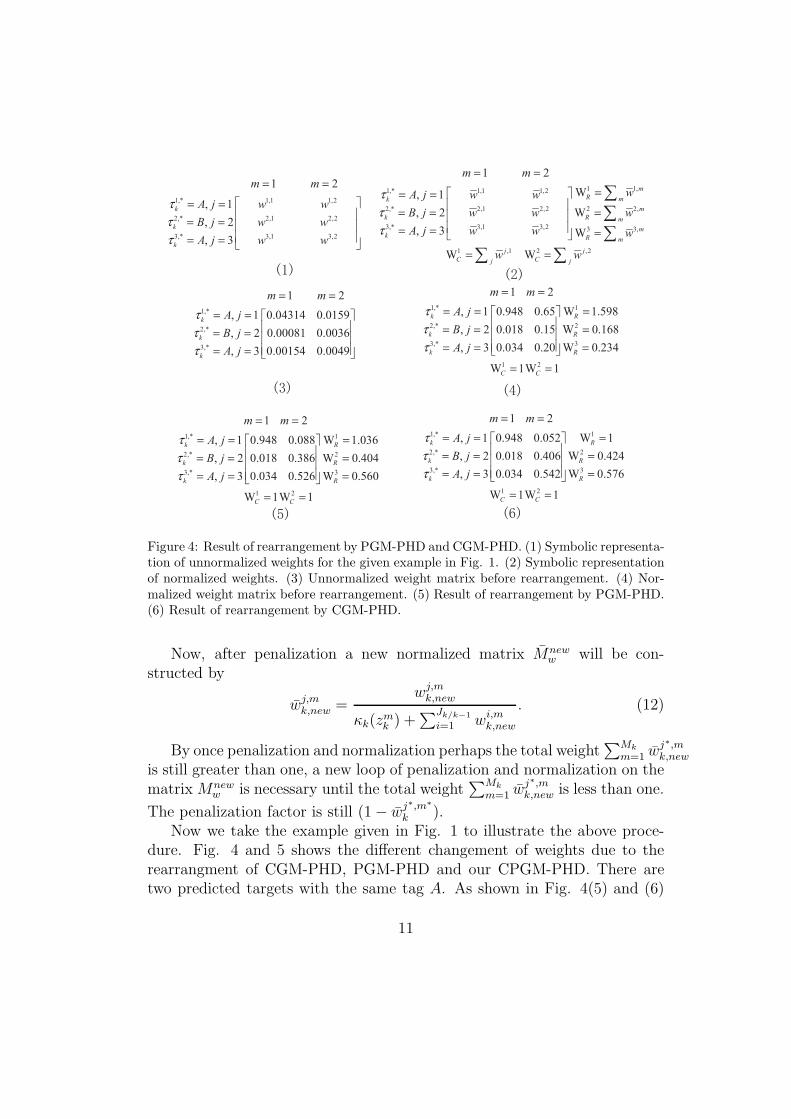
Figure 5: Numerical results after each step of processing in CPGM-PHD.

12

the target x3,2 achieves higher weight than x1,2, x2,2 by the rearrangementof PGM-PHD or PGM-PHD, and the two filters report the targets x1,1 andx3,2 as their estimations. However, x1,1 and x3,2 has the same tag A. Fig. 5shows the numerical results after each step of processing in CPGM-PHD andthe tracker finally reports the targets x1,1 and x2,2 as its estimations. Thefinal results are got by two penalizations on target A and one penalization ontarget B. The intermediate result after once penalization and renormaliza-tion as shown in Fig. 5(4) does not meet the condition of target consistencyfor W1

R > 1. It’s necessary to penalize again the weight matrix in Fig. 5(3).Finally the sum of all the weights in each row is less than one after renor-malization as shown in Fig. 5(8). Generally at most two penalizations onone target are enough.

Multiple loops of penalizations are equal to once penalization by a factorof (1− wj∗,m∗

k )n. We can simply explain that the total weight

∑Mk

m=1 wj∗,mk,new

is always being reduced by penalization once again and each new normalizedweight wj∗,m

k,new is no more than the old wj∗,mk .

Suppose ρ = 1 − wj∗,m∗

k and the set of predicted targets with the same

label as τ j∗,m∗

k is S, then

wj∗,mk,new − wj∗,m

k

=ρwj∗,m

k

κk(zmk ) +∑

i/∈S wi,mk + ρ

∑

i∈S wi,mk

−wj∗,m

k

κk(zmk ) +∑Jk/k−1

i=1 wi,mk

=(ρ− 1)wj∗,m

k

(

κk(zmk ) +

(∑

i/∈S wi,mk

))

(

κk(zmk ) +∑

i/∈S wi,mk + ρ

∑

i∈S wi,mk

)

(

κk(zmk ) +∑Jk/k−1

i=1 wi,mk

)

< 0.

So each new normalized weight wj∗,mk,new is no more than the old wj∗,m

k and

the total weight∑Mk

m=1 wj∗,mk,new is always being reduced by penalization and

renormalization once again.Besides, considering some spurious predicted targets perhaps achieve high

weights after renormalization so as to generate spurious trajectories, we limitthe rearrangement of weights on the steady trajectories. The estimationswith the same label at multiple time steps construct a trajectory. If thenumber of dots in some trajectory is very small, i.e., the trajectory is short,we keep its original weights unchanged for we don’t know the trajectory iswhether spurious or true.

13

Suppose the label set of steady trajectories is Ts, then the final weightmatrix Mfinal

w is recorded as

wj,mk,final =

{

wj,mk,new, ∀j = 1 : Jk/k−1, ∀m = 1 : Mk, τ

j,mk ∈ Ts

wj,mk ∀j = 1 : Jk/k−1, ∀m = 1 : Mk, τ

j,mk /∈ Ts.

(13)

If the label A of a new estimate belongs to the label set of the recordedtrajectories, we add one to the number of the tracking dots in the corre-sponding trajectory, else add the label A to the label set of the recordedtrajectories and record that the trajectory A has one tracking dot. The labelset of steady trajectories consists of the recorded trajectories which own atleast a certain amount of tracking dots, for instance, 5.

Remark: In some special scenarios targets are so close that multiple Gaus-sian components representing different targets are merged into one. It’simpossible to get estimations with different identities from such a mergedGaussian by any rearrangement of weights. In original GM-PHD tracker,the same identity would be assigned to multiple tracks evolved from such amerged Gaussian at next time step. It’s also improper to penalize the up-dated targets evolved from such a merged Gaussian in CPGM-PHD tracker.So we propose to record each target merged from multiple Gaussians withdifferent identities, and skip the rearrangement of weights on such a targetwith multiple hidden identities. If the targets are too close, the problem ofassigning the same identity to multiple tracks can’t still be well solved byany GM-PHD-based approach recently. However, we provide each track withhidden multiple identities in the hope to assist other means such as manualwork in judging the true identity of each track.

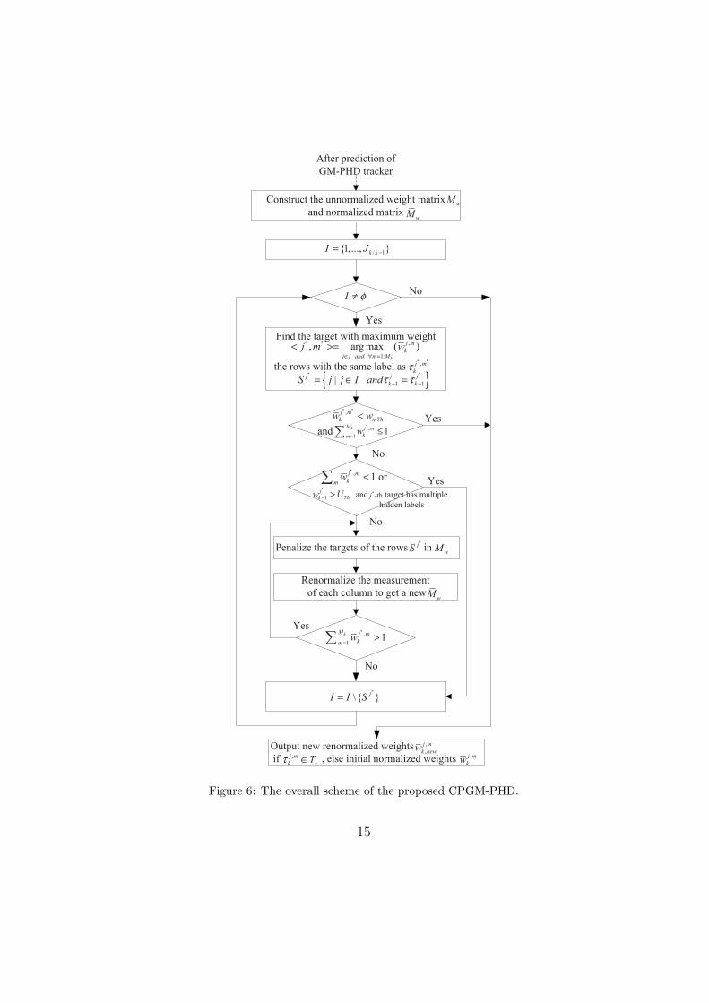
The overall scheme of our proposed CPGM-PHD tracker is illustrated asshown in Fig. 6. For τ j,mk = τ jk/k−1 = τ jk−1, we find the rows with the same

label as τ j∗,m∗

k when τ jk−1 = τ j∗

k−1.The CPGM-PHD tracker is summarized by the pseudo-code in Table 1-3.

4. Simulation results

For illustration purpose, we consider a Cartesian two-dimensional targettracking with a number of different probabilities of detection and clutterrates. The state xk = (px,k, px,k, py,k, py,k)

T of each target consists of its

position (px,k, py,k) and velocity (px,k, py,k), where [.]T denotes a transpose ofa matrix [.].

14

After prediction of

GM-PHD tracker

Construct the unnormalized weight matrix

and normalized matrix

I φ≠

/ 1{1,..., }k kI J −=

* * ,

1:

, arg max ( )k

j m

kj I and m M

j m w∈ ∀ =

< >=Find the target with maximum weight

* *,j m

k inThw w<

*j

Renormalize the measurement

of each column to get a new

*

\{ }jI I S=

Yes

No

No

Yes

Yes

wMwM

* ,

11

kM j m

kmw

=≤ and

Penalize the targets of the rows in

Yes

No

*, 1j m

kmw <

*

1

j

k Thw U− >

or

*-thjand target has multiple

hidden labels

* ,

11

kM j m

kmw

=>

No

the rows with the same label as* *,j m

kτ

{ }* *

1 1|j j j

k kS j j I andτ τ− −= ∈ =

*jS wM

wM

Output new renormalized weights

if , else initial normalized weights,j m

k sTτ ∈

,

,

j m

k neww,j m

kw

Figure 6: The overall scheme of the proposed CPGM-PHD.

15

Each target moves following the linear Gaussian model

xk =

1 T 0 00 1 0 00 0 1 T0 0 0 1

xk−1 +

T 2/2 0T 00 T 2/20 T

qk (14)

where qk is zero-mean Gaussian white noise with the varianceQ = diag([σ2v , σ

2v ]).

Each target generates an observation according to

zk =

[

1 0 0 00 0 1 0

]

xk + rk (15)

where rk is also zero-mean Gaussian white noise with the variance R =diag([σ2

ε , σ2ε ]).

The general parameters using the GM-PHD filter are as follows.The pruning threshold TTh = 10−5, merging threshold U = 4, weight

threshold wTh = 0.5, and maximum number of Gaussian components Jmax =100.

In addition, the special parameters for CPGM-PHD tracker include winTh =0.3 and UTh = 1.5.

Besides checking the tracking results of four trackers in one simulation, wefurther study the performance of the trackers using three criteria: accurateratio of identifying every target (described later), mean number of targetestimation error (NTE) [13, 22, 23] and mean optimal subpattern assignment(OSPA) [23, 25] between the estimated target set Xk and true target set Xk,where

NTE{Xk, Xk} = E{∣

∣

∣Xk

∣

∣

∣− |Xk|} (16)

OSPAp,c(Xk, Xk)

=

1∣

∣

∣Xk

∣

∣

∣

minπ∈Π|Xk|

|Xk|∑

i=1

(dc(xi, xπ(i)))

p+ cp × (

∣

∣

∣Xk

∣

∣

∣− |Xk|)

1/p

(17)

where the parameter p and c define the order and the cut-off value of theOSPA metric, and are set to 1 and 200 respectively [23, 25]. The distancedc(x, x) = min(c, d(x, x)) is the cut-off distance between the cut-off param-eter c and the Euclidean distance of the states x and x. The set Π|Xk|

16

represents the set of permutations of length∣

∣

∣Xk

∣

∣

∣with elements taken from

{1, 2, ...,∣

∣

∣Xk

∣

∣

∣}.

The simulations are performed in the following three scenarios illuminatedby different sensors to compare the performance of the proposed CPGM-PHDtracker with the original GM-PHD tracker, CGM-PHD tracker and PGM-PHD tracker. For the CGM-PHD filter and PGM-PHD filter do not providethe continuous trajectories of targets, we implement the two trackers byarranging labels to Gaussian mixture like GM-PHD tracker.

Scenario 1 is exactly the same as the scenario 1 in [22, 23]. The sensorilluminating scenario 1 has large measurement noise. In scenario 2 and 3 theprecision of the sensor is higher, but targets move more slow and are moreclose. So trajectories are perhaps wrongly identified in scenario 2 and 3.

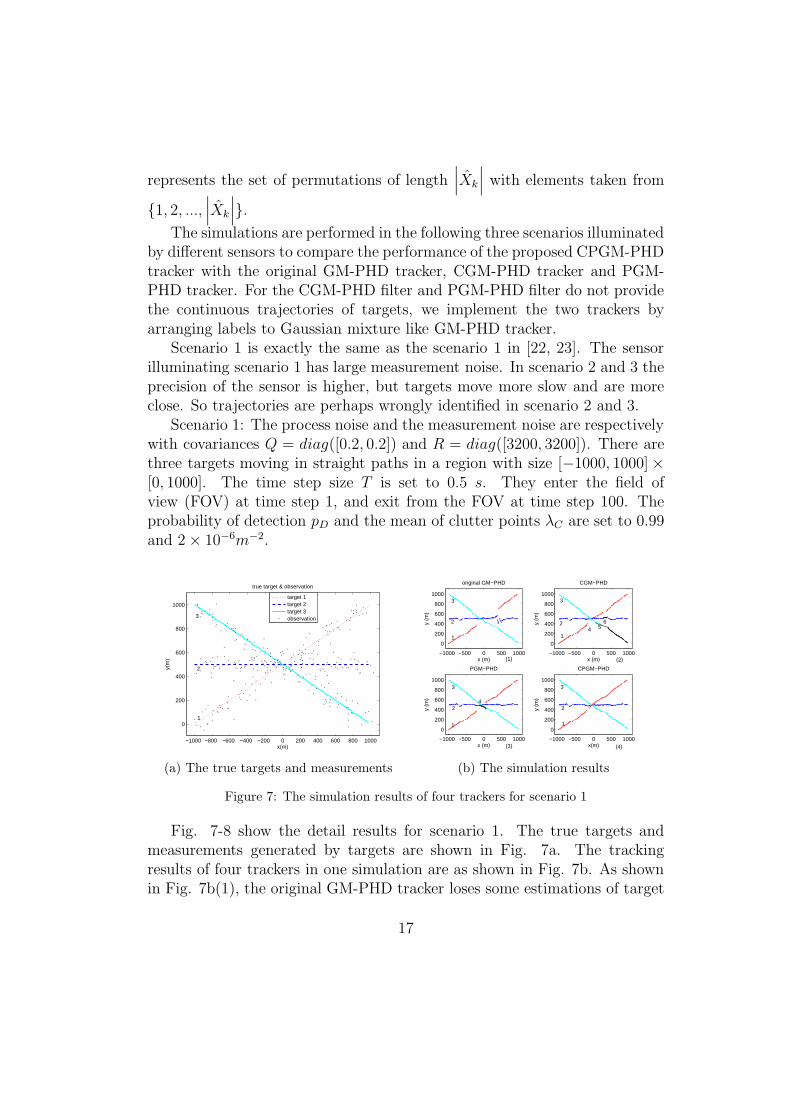
Scenario 1: The process noise and the measurement noise are respectivelywith covariances Q = diag([0.2, 0.2]) and R = diag([3200, 3200]). There arethree targets moving in straight paths in a region with size [−1000, 1000]×[0, 1000]. The time step size T is set to 0.5 s. They enter the field ofview (FOV) at time step 1, and exit from the FOV at time step 100. Theprobability of detection pD and the mean of clutter points λC are set to 0.99and 2× 10−6m−2.

−1000 −800 −600 −400 −200 0 200 400 600 800 1000

0

200

400

600

800

1000

x(m)

y(m

)

true target & observation

1

2

3

target 1target 2target 3observation

(a) The true targets and measurements

−1000 −500 0 500 1000

0

200

400

600

800

1000

1

2

3

y (m

)

x (m)

original GM−PHD

−1000 −500 0 500 1000

0

200

400

600

800

1000

1

2

3

4

y (m

)

x (m)

PGM−PHD

−1000 −500 0 500 1000

0

200

400

600

800

1000

1

2

3

4 56y

(m)

x (m)

CGM−PHD

−1000 −500 0 500 1000

0

200

400

600

800

1000

1

2

3

y (m

)

x(m)

CPGM−PHD

(1) (2)

(3) (4)

(b) The simulation results

Figure 7: The simulation results of four trackers for scenario 1

Fig. 7-8 show the detail results for scenario 1. The true targets andmeasurements generated by targets are shown in Fig. 7a. The trackingresults of four trackers in one simulation are as shown in Fig. 7b. As shownin Fig. 7b(1), the original GM-PHD tracker loses some estimations of target

17

20 30 40 50 60 70 800

0.5

1

time step

NT

E

20 30 40 50 60 70 8020

40

60

80

time step

OS

PA

GM−PHDCGM−PHDPGM−PHDCPGM−PHD

Figure 8: The simulation results of four trackers for scenario 1.

‘1’ for a while when three targets come near each other. Besides, severalestimations are a little off the true trajectory of target ‘2’. As shown in Fig.7b(2) and (3), some spurious estimations or trajectories are generated bythe CGM-PHD and PGM-PHD trackers, especially CGM-PHD tracker. Asshown in Fig. 7b(2), target ‘3’ is missing for a period and a new target ‘5’instead of target ‘3’ is wrongly generated. Fig. 7b(4) shows our proposedapproach provides the continuous and integrated trajectories of the threecrossing targets.

Fig. 8 demonstrates the corresponding results using NTE and OSPAin 100 runs. When targets are far from each other, the error rates of fourtrackers are nearly the same. For the clarity of the figure, we just alternativelyshow the results of time steps 20-80. When targets come near each other,for the original GM-PHD trackers whether NTE or OSPA is much higherthan the results of other improved trackers. The performance of the PGM-PHD and CGM-PHD trackers has improved significantly, while our proposedCPGM-PHD trackers has the lowest error rates all long.

Now we study the performance of our method in tracking more closetargets.

Scenario 2: In this scenario there are three targets moving in straightpaths in a region with size [−500, 500]× [−500, 500]. They enter the FOV attime step 1, and exit from the FOV at time step 100.

18

Scenario 3: In this scenario the FOV is also with size [−500, 500] ×[−500, 500]. Two targets enter the FOV at time step 1 and move towardseach other until time step 75 before they meet. After that, the targets goaway from each other and exit from the FOV at time step 150.

For the two scenarios above we set the process noise σv = 1(m/s2) andthe observation noise σε = 16m respectively in all simulations. The time stepsize T is set to 1 s. Each target has survival probability ps,k = 0.99 at eachtime step.

−500 −400 −300 −200 −100 0 100 200 300 400 500−500

−400

−300

−200

−100

0

100

200

300

400

500

x(m)

y(m

)

true target & observation

target 1target 2target 3observation

2

1

3

(a) The true targets and measurements

−500 0 500−500

0

500

3

2

1

y (m

)x (m)

original GM−PHD

−500 0 500−500

0

500

3

2

1

y (m

)

x (m)

CGM−PHD

−500 0 500−500

0

500

3

2

1

y (m

)

x (m)

CPGM−PHD

−500 0 500−500

0

500

3

2

1

y (m

)

x (m)

PGM−PHD

(1) (2)

(3) (4)

(b) The simulation results

Figure 9: The simulation results of four trackers for scenario 2

−500 −400 −300 −200 −100 0 100 200 300 400 500

−500

−400

−300

−200

−100

0

100

200

300

400

500

x(m)

y(m

)

true target & observation

target 1target 2observation

1

2

(a) The true targets and measurements

−500 0 500−500

0

500

2

1

y (m

)

x (m)

original GM−PHD

−500 0 500−500

0

5002

1

y (m

)

x (m)

CGM−PHD

−500 0 500−500

0

500

2

1

y (m

)

x (m)

PGM−PHD

−500 0 500−500

0

500

2

1

y (m

)

x (m)

CPGM−PHD

(1) (2)

(3) (4)

(b) The simulation results

Figure 10: The simulation results of four trackers for scenario 3

Fig. 9a shows an example of three crossing targets for scenario 2. Twoof the three targets cross in turn. The three targets are with velocities in

19

y axis respectively v1y = 8m/s, v2y = 0, v3y = −8m/s and all have the samevelocity in x axis vx = 10m/s. The probability of detection pD and the meanof clutter points λC are set to 0.99 and 10× 10−6m−2, respectively.

Fig. 9b(1) shows that for GM-PHD tracker there are three target trajec-tories after targets cross, but the same identity ‘2’ is assigned to two of thethree trajectories. That is, GM-PHD tracker can not distinguish betweentarget ‘2’ and target ‘3’ when they come near each other. Much the sameresults are got by the PGM-PHD trackers as shown in Fig. 9b(3). Fig. 9b(2)shows that the CGM-PHD tracker can’t also distinguish between the threetargets and identities are wrongly assigned after targets cross. Target ‘2’ iswrongly identified and the same identity ‘1’ is assigned to two trajectories.

Fig. 9b(4) shows our proposed approach provides the continuous andsmooth trajectories with correctly identifying the three crossing targets.

Remark: According to the tracking scheme of GM-PHD, we should choosethe branch with the largest weight from multiple branches owning the sametag as the estimation of each target. However, for perhaps the assignmentof the same identity to multiple tracks when targets come near each other,there would result in missing some estimations if choosing only one frommultiple estimations with the same tag. So we output all the estimationswith weights wk > wTh to more precisely estimate the number of targets. Itcan still evaluate the estimation performance by analyzing NTE and OSPA.

Fig. 10a shows another example of two closely spaced targets for scenario3. The two targets have the same velocity in x axis vx = 6.7m/s, and initialvelocities in y axis respectively v1y = 10m/s, v2y = −10m/s. They move withconstant velocity in x axis. In y axis the two targets respectively experienceconstant speed until time step 21, then constant deceleration or accelarationuntill time step 129 with accelarations a1y = −0.185m/s2, a2y = 0.185m/s2,and then constant speed until time step 150. The probability of detectionpD and the mean of clutter points λC are also set to 0.99 and 10× 10−6m−2,respectively.

Fig. 10b(1) shows that the GM-PHD tracker assigns the same identity‘2’ to both targets after the two targets become close and separate then. TheCGM-PHD tracker and PGM-PHD tracker fail to correctly keep the separateidentities of target ‘1’ and target ‘2’ as shown in Fig. 10b(2) and (3).

Besides, due to improper weight adjustment the CGM-PHD tracker andPGM-PHD tracker generate a few spurious target estimations as a result thattrajectories of targets fluctuate when targets become close.

Fig. 10b(4) shows the results of our proposed approach which resolves

20

the identities of the two targets and there are no large fluctuations in thetrajectories of targets.

20 30 40 50 60 70 800

0.2

0.4

0.6

0.8

time step

NT

E

20 30 40 50 60 70 80

20

40

60

time step

OS

PA

GM−PHDCGM−PHDPGM−PHDCPGM−PHD

(a) Results for scenario 2

30 40 50 60 70 80 90 100 110 1200

0.1

0.2

0.3

time step

NT

E

30 40 50 60 70 80 90 100 110 12010

20

30

40

time step

OS

PA

GM−PHDCGM−PHDPGM−PHDCPGM−PHD

(b) Results for scenario 3

Figure 11: NTE and OSPA of four trackers

A Monte Carlo simulation with 100 runs is employed to evaluate theperformance of the trackers using NTE and OSPA. Fig. 11a and 11b demon-strate the corresponding results of different trackers for scenario 2 and 3. Theprobability of detection pD and the mean of clutter points per unit area λC

are set to 0.99 and 10× 10−6m−2. For scenario 2, the performance of PGM-PHD tracker and CGM-PHD tracker has improved greatly as shown in Fig.11a, but for scenario 3 both improved trackers make little improvement oferror rates as shown in Fig. 11b. For the two scenarios, it can be seen thatour proposed CPGM-PHD tracker all along has the lower error rates thanthe other three trackers.

In order to study the performance of our proposed method in higheruncertainties and make comparison with the other trackers, we provide theresults of four trackers for the two scenarios above in various clutter rates andprobabilities of detection. For each configuration, a Monte Carlo simulationwith 200 runs is employed to obtain reliable results. The metrics of NTEand OSPA are computed at each time step for 200 runs and then over time.

Fig. 12a and 12b illustrate the averaged NTE and OSPA respectively fortracking targets in scenario 2. The horizontal axes in fig. 12a (1) and 12b (2)show the mean of clutter points per unit area λC . So the number of clutterpoints per frame is equal to λC × V , where V = 106m2 is the area of theFOV for scenario 2.

For different clutter rates, the probability of detection pD is set to 0.99,

21

0 0.5 1 1.5

x 10−5

0

0.05

0.1

0.15

0.2

0.25

0.3

0.35

Clutter Rate

NT

E (

Ave

rage

d on

Tim

e)

GM−PHDCGM−PHDPGM−PHDCPGM−PHD

0.8 0.85 0.9 0.95 10

0.1

0.2

0.3

0.4

0.5

0.6

0.7

Probability Detection

NT

E (

Ave

rage

d on

Tim

e)

(1) (2)

(a) Averaged NTE

0 0.5 1

x 10−5

12

14

16

18

20

22

24

26

28

30

Clutter Rate

OS

PA

(A

vera

ged

on T

ime)

GM−PHDCGM−PHDPGM−PHDCPGM−PHD

0.8 0.85 0.9 0.95 110

15

20

25

30

35

40

45

50

55

Probability Detection

OS

PA

(A

vera

ged

on T

ime)

(1) (2)

(b) Averaged OSPA

Figure 12: Averaged NTE and OSPA of tracking three targets (scenario 2) in terms ofdifferent clutters and probabilities of detection.

0 0.5 1 1.5

x 10−5

0.02

0.04

0.06

0.08

0.1

0.12

0.14

0.16

0.18

0.2

Clutter Rate

NT

E (

Ave

rage

d on

Tim

e)

GM−PHDCGM−PHDPGM−PHDCPGM−PHD

0.8 0.85 0.9 0.95 10

0.05

0.1

0.15

0.2

0.25

0.3

0.35

0.4

0.45

Probability Detection

NT

E (

Ave

rage

d on

Tim

e)

(1) (2)

(a) Averaged NTE

0 0.5 1 1.5

x 10−5

12

14

16

18

20

22

24

26

Clutter Rate

OS

PA

(A

vera

ged

on T

ime)

GM−PHDCGM−PHDPGM−PHDCPGM−PHD

0.8 0.85 0.9 0.95 110

15

20

25

30

35

40

45

50

55

Probability Detection

OS

PA

(A

vera

ged

on T

ime)

(1) (2)

(b) Averaged OSPA

Figure 13: Averaged NTE and OSPA of tracking two targets (scenario 3) in terms ofdifferent clutters and probabilities of detection.

and for different probabilities of detection the clutter rate is fixed on λC =10× 10−6m−2.

Fig. 12a (1) and Fig. 12b (1) show that the CGM-PHD tracker andPGM-PHD tracker achieve the similar error rates which are lower than thatof the orginal GM-PHD tracker. As shown in Fig. 12a (2) and Fig. 12b(2) when probability of detection tends to decrease, estimation error of alltrackers tends to rise. For the same probability of detection, the CGM-PHDtracker and PGM-PHD tracker achieve almost the same error rates, so the

22

results of both trackers look like one curve.Whenever our proposed CPGM-PHD tracker has the lowest error rates

for all of the clutter rates and probabilities of detection as shown in Fig. 12aand 12b.

Fig. 13a and 13b illustrate the averaged NTE and OSPA respectively fortracking two closely spaced targets in scenario 3. The configuration of pD andλC is the same to that for scenario 2. Similar to the results of scenario 2, ourproposed method has the lowest error rates in all simulations for scenario3 as shown in Fig. 13a and 13b. The order of descending error rates isthe original GM-PHD tracker, CGM-PHD tracker, PGM-PHD tracker andCPGM-PHD tracker.

Now we study the important performance of correctly identifying closetargets for four trackers.

The accurate rate of identifying every target is defined as the percentage oftimes quite correctly identifying and continuously tracking every target overmultiple runs. For every simulation, we record the number of estimations ineach trajectory with the same tag. According to the features of the scenarioswe study, we propose to define that the tracking results need to satisfy thefollowing two conditions so as that we recognize that the trackers correctlyidentify every target.

(1) The number of long trajectories owning at least (pD×n−mo) trackingpoints is equal to the true number of targets where pD is probability ofdetection, n is the total time step (n = 100 for scenario 2, and scenairo 3n = 150) and mo is the given offset number (mo = 25 for both scenarios).

(2) The distance De of the first point and last point in the long trajectorymentioned above is near to that of true trajectory. Record the true distanceDt of the first point and last point for target ‘1’. For scenario 2 there aretwo tracks with De more than (Dt − 150), and for scenario 3 there are twotracks with De less than (Dt + 50).

Fig. 14a shows the accurate rates of tracking three targets for scenario2 in terms of different clutters and probabilities of detection over 200 runs.As shown in Fig. 14a the CGM-PHD tracker and PGM-PHD tracker havesubstantially improved the performance of the GM-PHD tracker in correctlyidentifying close targets, while our proposed approach has higher accuraterate in all configurations and the accurate rates have been raised at least 20percent compared with the CGM-PHD tracker and PGM-PHD tracker. Ofcourse when probability of detection tends to decrease, the accurate rate ofour proposed approach also tends to decrease. However, the accurate rate is

23

0 0.5 1 1.5

x 10−5

0.1

0.2

0.3

0.4

0.5

0.6

0.7

0.8

0.9

1

Clutter Rate

Acc

urat

e R

ate

GM−PHDCGM−PHDPGM−PHDCPGM−PHD

0.8 0.85 0.9 0.95 10.1

0.2

0.3

0.4

0.5

0.6

0.7

0.8

0.9

1

Probability Detection

Acc

urat

e R

ate

(1) (2)

(a) results for scenario 2

0 0.5 1 1.5

x 10−5

0.4

0.5

0.6

0.7

0.8

0.9

1

Clutter Rate

Acc

urat

e R

ate

GM−PHDCGM−PHDPGM−PHDCPGM−PHD

0.8 0.85 0.9 0.95 1

0.4

0.5

0.6

0.7

0.8

0.9

1

Probability Detection

Acc

urat

e R

ate

(1) (2)

(b) results for scenario 3

Figure 14: Accurate rate in terms of different clutter rates and probabilities of detection.

improved at least 20 percent compared with the CGM-PHD and PGM-PHDtracker in terms of different probabilities of detection.

Fig. 14b shows the accurate rates of tracking two closely spaced targetsfor scenario 3 over 200 runs. When clutter intensity is small, three improvedtrackers all can identify each target at high accurate rates. However, whenthere are dense clutter, the performances of the CGM-PHD and PGM-PHDtracker dramatically decrease. Especially the CGM-PHD tracker results inlower accurate rate than the original GM-PHD tracker. In all simulationsthe CPGM-PHD tracker has the highest accurate rates of identifying closetargets. For different clutter rates the accurate rates of CPGM-PHD trackerare more than 90 percent. For different probability of detections the accuraterates of CPGM-PHD tracker are more than 80 percent.

When probability of detection is small, our approach can’t also achieveperfect performance of correctly identifying close targets. When targets be-come close, due to missing of measurements the phenomenon that the dis-tances of more than one measurement towards one target are smaller thanthat towards other targets happens rarely. So our approach based on rear-ranging the weights of inconsistent targets can’t make effect due to missingof measurements.

5. Conclusion

In order to improve the performance of GM-PHD-based filter for trackingclosely space targets, a novel approach called collaborative penalized GM-

24

PHD (CPGM-PHD) tracker is proposed. The proposed approach utilizesthe one-to-one correspondence between each measurement and each targetwith different identity to collaboratively penalize the weights of targets. Bypenalization and renormalization the original weak targets are highlighted.

The simulation results in terms of various probabilities of detection andclutter rates show that the proposed CPGM-PHD tracker has a better per-formance in identity confirmation than the original GM-PHD tracker, CGM-PHD tracker and PGM-PHD tracker, and the estimation accuracy of targetnumber and states is also improved.

As the future work, our research plan is to apply our approach in morescenarios in which targets are more closer considering the separation distancesof target estimations.

References

[1] Y. Bar-Shalom, T. Fortmann, Tracking and Data Association, AcademicPress, Boston, 1988.

[2] S. Blackman, R. Popoli, Design and Analysis of Modern Tracking Sys-tems, Artech House, Boston, 1999.

[3] K.-C. Chang, C.-Y. Chong, Y. Bar-Shalom, Joint probabilistic data as-sociation in distributed sensor networks, IEEE Trans. Automatic Con-trol 31 (1986) 889–897.

[4] T. Fortmann, Y. Bar-Shalom, M. Scheffe, Sonar tracking of multiple tar-gets using joint probabilistic data association, IEEE Journal of OceanicEngineering 8 (1983) 173–184.

[5] S. Blackman, Multiple hypothesis tracking for multiple target tracking,IEEE Aerospace and Electronic Systems Magazine 19 (2004) 5–18.

[6] R. Mahler, Global integrated data fusion, in: Proc. Seventh NationalSymp. On Sensor Fusion, Sandia National Laboratories, Albuquerque,pp. 187–199.

[7] I. Goodman, R. Mahler, H. Nguyen, Mathematics of Data Fusion,Kluwer Academic Publishers, Boston, 1997.

25

[8] R. Mahler, Multitarget bayes filtering via first-order multitarget mo-ments, IEEE Trans. Aerospace and Electronic Systems 39 (2003) 1152–1178.

[9] R. Mahler, A theoretical foundation for the stein-winter probability hy-pothesis density (phd) multi-target tracking approach, in: Proc. 2000MSS National Symp. on Sensor and Data Fusion, volume 1(Unclassi-fied), Sandia National Laboratories, San Antonio TX, pp. 99–117.

[10] B.-N. Vo, S. Singh, A. Doucet, Sequential monte carlo methods formulti-target filtering with random finite sets, IEEE Trans. Aerospaceand Electronic Systems 41 (2005) 1224–1245.

[11] H. Sidenbladh, Multi-target particle filtering for the probability hypoth-esis density, in: Proceedings of Fusion, Cairns, Australia, pp. 1110–1117.

[12] T. Zajic, R. Mahler, A particle-systems implementation of the phdmulti-target tracking filter, in: Signal Processing, Sensor Fusion andTarget Recognition XII, SPIE Proc., volume 5096, pp. 291–299.

[13] B.-N. Vo, W. Ma, The gaussian mixture probability hypothesis densityfilter, IEEE Trans. Signal Processing 54 (2006) 4091–4104.

[14] K. Panta, B.-N. Vo, S. Singh, Novel data association schemes for theprobability hypothesis density filter, IEEE Trans. Aerospace and Elec-tronic Systems 43 (2007) 556–570.

[15] Y. Wang, Z. Jing, S. Hu, Data association for phd filter based on mht,in: 11th International Conference on Information Fusion, pp. 1–8.

[16] D. Clark, J. Bell, Data association for the phd filter, in: Proceedingsof Intelligent Sensors, Sensor Networks and Information Processing, pp.217–222.

[17] K. Panta, B.-N. Vo, D. Clark, An efficient track management schemefor the gaussian-mixture probability hypothesis density tracker, in: Pro-ceedings of the Fourth International Conference on Intelligent Sensingand information processing, pp. 15–18.

[18] K. Panta, D. Clark, B.-N. Vo, Data association and track managementfor the gaussian mixture probability hypothesis density filter, IEEETrans. Aerospace and Electronic Systems 45 (2009) 1003–1016.

26

[19] D. Clark, Multiple target tracking with the probability hypothesis den-sity filter, Ph.D. thesis, Heriot-Watt University, 2006.

[20] Y. Wang, H. Meng, H. Zhang, X. Wang, Track probability hypothesisdensity filter for multi-target tracking, in: Radar Conference (RADAR),2011 IEEE, pp. 612–615.

[21] M. Yazdian-Dehkordi, Z. Azimifar, M. Masnadi-Shirazi, An improve-ment on gm-phd filter for occluded target tracking, in: Proc. IEEE36th Int. Conf. on Acoustics, Speech and Signal Processing (ICASSP),pp. 1773–1776.

[22] M. Yazdian-Dehkordi, Z. Azimifar, M. Masnadi-Shirazi, Competitivegaussian mixture probability hypothesis density filter for multiple targettracking in the presence of ambiguity and occlusion, IET Radar, Sonar& Navigation 6 (2012) 251–262.

[23] M. Yazdian-Dehkordi, Z. Azimifar, M. Masnadi-Shirazi, Penalized gaus-sian mixture probability hypothesis density filter for multiple targettracking, Journal of Signal Processing 92 (2012) 1230–1242.

[24] M. Yazdian-Dehkordi, O. Roihani, Z. Azimifar, Visual target trackingin occlusion condition: a gm-phd based approach, in: 2012 16th CSIInt. Sym. on Artificial Intelligence and Signal Processing, pp. 538–541.

[25] D. Schuhmacher, B.-T. Vo, B.-N. Vo, A consistent metric for perfor-mance evaluation of multi-object fitlers, IEEE Trans. Signal Processing56 (2008) 3447–3457.

27

Table 1: Pseudo-Code for the CPGM-PHD trackerStep 0. Initializations. Given X0 =

{

wj0, m

j0, P

j0 , τ

j0

}

and SI0 =

{

Ij0}

,

∀j = 1 : J0. τj0 is identity tag. Ij0 is hidden identity set of the j-th target.

set k = 1. Given Zk = {zmk } , ∀m = 1 : Mk.Step 1. Prediction

Step 1.1 Prediction for born targets

Xγ,k/k−1 ={

wjr,k, m

jr,k, P

jr,k, τ

jr,k

}

, ∀j = 1 : Jr,k. τjr,k are new tags.

Step 1.2 Prediction for spawned targets Xβ,k/k−1 (details omitted)Step 1.3 Prediction for survived targets

for j = 1 : Jk−1

wjS,k/k−1 = pS,kw

jk−1; mj

S,k/k−1 = Fk−1mjk−1;

P jS,k/k−1 = Qk−1 + Fk−1P

jk−1F

Tk−1; τ jS,k/k−1 = τ jk−1;

end

XS,k/k−1 ={

wjS,k/k−1, m

jS,k/k−1, P

jS,k/k−1, τ

jS,k/k−1

}

, ∀j = 1 : Jk−1;

Xk/k−1 = XS,k/k−1

⋃

Xγ,k/k−1

⋃

Xβ,k/k−1;

Ijk/k−1 = Ijk−1, ∀j = 1 : Jk−1; Ijk/k−1 = τ jk/k−1, ∀j > Jk−1;

Step 2. Construction of PHD update componentsfor j = 1 : Jk/k−1

zjk/k−1 = Hkmjk/k−1;S

jk = Rk +HkP

jk/k−1H

Tk ;K

jk = P j

k/k−1HTk (S

jk)

−1;

endStep 3. Update

Step 3.1. Update for undetected targetsfor j = 1 : Jk/k−1

wjk = (1− pD,k)w

jk/k−1;m

jk = mj

k/k−1;Pjk = P j

k/k−1; τjk = τ jk/k−1; I

jk = Ijk/k−1;

end

Xm,k ={

wjk, m

jk, P

jk , τ

jk

}

, ∀j = 1 : Jk/k−1;Step 3.2. Update for detected targets

for m = 1 : Mk

for j = 1 : Jk/k−1

wj,mk = pD,kw

jk/k−1N(zmk ; zjk/k−1, S

jk);

mj,mk = mj

k/k−1 +Kjk(z

mk − zjk/k−1);

P j,mk = (I −Kj

kHk)Pjk/k−1; τ j,mk = τ jk/k−1;

end

wj,mk =

wj,mk

κk(zmk )+

∑Jk/k−1

j=1wj,m

k

, ∀j = 1 : Jk/k−1;

end

wj,mk,old = wj,m

k , ∀j = 1 : Jk/k−1, m = 1 : Mk;28

Table 2: Pseudo-Code for the CPGM-PHD tracker ((Continued from previous table))

I = {1, ..., Jk/k−1};While I 6= ∅

Step a. Find the target with maximum weight

< j∗, m∗ >= argmaxj∈I and ∀m=1:Mk

(wj,mk );

if wj∗,m∗

k < winTh and∑Mk

m=1 wj∗,mk ≤ 1

break;end

Step b. Find the targets with the same label as τ j∗,m∗

k

(equal to τ j∗

k−1)

Sj∗ ={

i∣

∣

∣τ ik−1 = τ j

∗

k−1, i ∈ I}

;

if∑Mk

m=1 wj∗,mk ≤ 1 or (wj∗

k−1 > UTh and card(Ij∗

k/k−1) > 1)

I = I \ {Sj∗};else

While∑Mk

m=1 wj∗,mk > 1

Step c. Penalize the weights of targets in Sj∗

except the measurement m∗

ρ = 1− wj∗,m∗

k ;for m = 1 : Mk

if m 6= m∗

wj,mk = wj,m

k ∗ ρ, ∀j ∈ Sj∗;end

endStep d. Apply weight renormalizationfor m = 1 : Mk

wj,mk =

wj,mk

κk(zmk )+

∑Jk/k−1

i=1wi,m

k

, ∀j = 1 : Jk/k−1;

end

end (% end While∑Mk

m=1 wj∗,mk > 1)

I = I \ {Sj∗};end

end (% end While I 6= ∅ )Step e. Keep the old weight of unsteady trajectories unchanged

wj,mk = wj,m

k,old, ∀j = 1 : Jk/k−1, ∀m = 1 : Mk, τjk-1 /∈ Ts;

Xd,k ={

wj,mk , mj,m

k , P j,mk , τ j,mk

}

, Ij,mk = Ijk/k−1, ∀j = 1 : Jk/k−1, ∀m = 1 : Mk;

Xk = Xm,k

⋃

Xd,k = {wik, m

ik, P

ik, τ

ik} , S

Ik =

{

Ijk}

, ∀i = 1 : Jk;

29

Table 3: Pseudo-Code for the CPGM-PHD tracker ((Continued from previous table))

Step 4. Pruning and MergingGiven a truncation threshold TTh, a merging threshold U ,and a maximum allowable number of Gaussian components Jmax,set l = 0, and I = {i = 1, ..., Jk |w

ik > TTh}, repeat

l = l + 1;j = argmax

i∈Iwi

k;

L ={

i ∈ I∣

∣

∣(mi

k −mjk)

T(P i

k)−1(mi

k −mjk) ≤ U

}

;

wlk =

∑

i∈L

wik; m

lk =

1wl

k

∑

i∈L

wikm

ik;

P lk = 1

wlk

∑

i∈L

wik

[

P ik + (ml

k −mik)(m

lk −mi

k)T]

;τ lk = τ jk ;

Record the hidden identities in descending order of possibilityI lk = ∅;[w,OL] = sort ({wi

k|i ∈ L} ,′ descend′);for i = 1 : len(OL)

if wOL(i) < 0.1break;

else

I lk = I lk⋃

IOL(i)k ;

endendI := I\L;

until I = ∅.

if l > Jmax replace{

wjk, m

jk, P

jk , τ

jk

}

and{

Ijk

}

, ∀j = 1 : l by those of the

Jmax Gaussian with largest weights. Xk ={

wjk, m

jk, P

jk , τ

jk

}

and SIk =

{

Ijk

}

, ∀j = 1 : l.

Output.{

wjk, m

jk, P

jk , τ

jk

∣

∣wjk > wTh

}

, ∀j = 1 : l.

Record the label set of steady trajectories.(details omitted for lack of space).

30