Multi-objective optimization algorithms for mixed model ... · Multi-objective optimization algorithms for mixed model assembly line balancing problem with parallel workstations ...

Page 1 of 19

PRODUCTION & MANUFACTURING | RESEARCH ARTICLE

Multi-objective optimization algorithms for mixed model assembly line balancing problem with parallel workstationsMasoud Rabbani, Reyhaneh Siadatian, Hamed Farrokhi-Asl and Neda Manavizadeh

Cogent Engineering (2016), 3: 1158903

Rabbani et al., Cogent Engineering (2016), 3: 1158903http://dx.doi.org/10.1080/23311916.2016.1158903

PRODUCTION & MANUFACTURING | RESEARCH ARTICLE

Multi-objective optimization algorithms for mixed model assembly line balancing problem with parallel workstationsMasoud Rabbani1*, Reyhaneh Siadatian1, Hamed Farrokhi-Asl2 and Neda Manavizadeh3

Abstract: This paper deals with mixed model assembly line (MMAL) balancing problem of type-I. In MMALs several products are made on an assembly line while the similarity of these products is so high. As a result, it is possible to assemble several types of products simultaneously without any additional setup times. The problem has some particular fea-tures such as parallel workstations and precedence constraints in dynamic periods in which each period also effects on its next period. The research intends to reduce the number of workstations and maximize the workload smoothness between workstations. Dynamic periods are used to determine all variables in different periods to achieve efficient solutions. A non-dominated sorting genetic algorithm (NSGA-II) and multi-objective particle swarm optimization (MOPSO) are used to solve the problem. The proposed model is validated with GAMS software for small size problem and the performance of the foregoing algorithms is compared with each other based on some comparison metrics. The NSGA-II outperforms MOPSO with respect to some comparison metrics used in this paper, but in other metrics MOPSO is better than NSGA-II. Finally, conclusion and future research is provided.

Subjects: Industrial Engineering & Manufacturing; Manufacturing Engineering; Production Engineering

Keywords: multi-objective optimization; mixed model assembly lines; balancing; sequencing; parallel workstations

*Corresponding author: Masoud Rabbani, School of Industrial Engineering, College of Engineering, University of Tehran, P.O. Box 11155-4563 Tehran, Iran E-mail: [email protected]

Reviewing editor:Zude Zhou, Wuhan University of Technology, China

Additional information is available at the end of the article

ABOUT THE AUTHORSMasoud Rabbani is a professor of Industrial Engineering in the School of Industrial and Systems Engineering at the University of Tehran.

Reyhaneh Siadatian is MSc degree student in school of Industrial Engineering at university of Tehran.

Hamed Farrokhi-Asl finished his Bachelor of Science in Industrial Engineering from University of Khaje-Nasir University of Technology, Iran at 2013. He continued his master’s studies at University of Tehran and graduated at 2014.

Neda Manavizadeh obtained her PhD in Industrial Engineering from College of Engineering, University of Tehran (Start year: 2008). Currently, she is an assistant professor at Industrial Engineering Department, KHATAM University, Tehran, Iran.

PUBLIC INTEREST STATEMENTIn today’s highly competitive industrial environment, increasing systems’ flexibility to meet customers’ demands is crucial. Assembly line is a flow of materials subjected to workstations. In mixed model assembly lines several products are made on an assembly line while the similarity of these products is so high. As a result, it is possible to assemble and produce several types of products simultaneously in rational time. So, the flexibility of this type of the assembly line is high to produce different product with high volume based on customers’ demand. This paper deals with the mixed model assembly line balancing problem where the parallel workstations in dynamic periods are considered. Dynamic periods means that each period has effects on its next period, and this is used to increase efficiency of the line. Two algorithms are used to solve the proposed mathematical model and the results are compared with each other.

Received: 19 October 2015Accepted: 17 February 2016First Published: 03 March 2016

© 2016 The Author(s). This open access article is distributed under a Creative Commons Attribution (CC-BY) 4.0 license.

Page 2 of 19

Masoud Rabbani

Page 3 of 19

Rabbani et al., Cogent Engineering (2016), 3: 1158903http://dx.doi.org/10.1080/23311916.2016.1158903

1. IntroductionAssembly line is a flow of materials and components subjected to workstations placed as a sequence. As parts move through this line of production, they are assembled together or to the main part in order to form the final products. One of the models used in this kind of line, is a hybrid model called mixed model assembly line (MMAL) (Soman, van Donk, & Gaalman, 2004). In MMALs several products are made on an assembly line while the similarity of these products is so high that the setup time for stations from one product to another one is assumed to be negligible. As a result, it is possible to assemble several types of products simultaneously with respect to orders entered to the line without any additional setup times. A variety of similar models in MMAL can meet the various demands of customers. In today’s highly competitive manufacturing environment, increasing flexi-bility of systems according to customers ’ desires is crucial. MMAL has several advantages, such as products manufacturing based on customers demand and increasing the flexibility of the line. As a result, it is so important to study and search about this topic (Manavizadeh, Hosseini, Rabbani, & Jolai, 2013).

According to the above mentioned, if several products with high workload come to a workstation consecutively, they may increase the cycle time. To prevent this happening, concepts of balance and sequence are used. Sequencing assembly line includes the order of products entering the assembly line and whenever several models come with high volume followed at a station, the cycle time may exceed the station (Boysen, Fliedner, & Scholl, 2009). Assembly line balancing emerges when de-signing an assembly line and it consists of finding a feasible assignment of tasks to workstations in such a path that the assembly costs are minimized, the demand is met and constraints of the as-sembly process are satisfied (Boysen, Fliedner, & Scholl, 2007). As a result, the aim of the assembly line balancing is optimal assignment of works to stations.

There are some models used in assembly line balancing problem. The first of them which is used in this study is called assembly balancing problem type-I. It consists of assignment of tasks to work-stations where the number of workstations should be minimized for a given cycle time. The second types of assembly balancing problem is type-II and it occurs when there are certain numbers of workstations, but the cycle time is unknown (Akpınar & Bayhan, 2011).

The rest of the paper is organized as follows: in Section 2, some related literatures are reviewed. Mathematical model and the problem definition are presented in Section 3. The concept of a non-dominated solution is illustrated in Section 4. In Section 5, the methodology for tackling of this problem is described. Numerical results and comparison of two metaheuristics are presented in Section 6. Finally, the study is ended with the conclusion in Section 7.

2. Literature reviewMcMullen and Frazier (1998) found that using equal weight for each objective to solve a multi-objec-tive assembly line balancing problem with simulated annealing algorithm when workstations are parallel has a better result. Simaria and Vilarinho (2004) solved MMAL balancing problem type-II with genetic algorithm to find the best balance in parallel workstations while the problem had con-straints of zoning. McMullen and Tarasewich (2003) used ant techniques to solve the MMAL balanc-ing problem with parallel workstations and probable time work. They compared ant techniques with several other heuristics, such as simulated annealing and found that this approach is competitive with the other methods.

Simaria and Vilarinho (2009) solved balancing two-sided assembly lines problem with an ant col-ony optimization algorithm to minimize number of workstations and balancing the workload with precedence, capacity, zoning, and synchronism constraints. They understood that their proposed procedure is performed well. Rabbani, Kazemi, and Manavizadeh (2012) proposed a new approach to minimize the number of workstations when these are intersecting in mixed model U-line balanc-ing type-I problem and solved it with genetic algorithm. Hamzadayi and Yildiz (2012) used genetic algorithm and simulated annealing to solve MMAL balancing type-I problem with sequence in U-line

Page 4 of 19

Rabbani et al., Cogent Engineering (2016), 3: 1158903http://dx.doi.org/10.1080/23311916.2016.1158903

with parallel workstations and zoning constraints. Boysen, Kiel, and Scholl (2011) focused on the added workload stations in sequencing MMAL and tried to minimize the number of work overload situations. They introduced different exact and heuristic algorithms such as branch and bound and tested their model in some instances.

Mamun, Khaled, Ali, and Chowdhury (2012) proposed a genetic algorithm to solve balancing mixed model assembly line of type-I with some features such as parallel workstations, zoning con-straints, and sequence with limit resources. They defined reassignment process to increase flexibility in task allocation. Tiacci (2012) evaluated operational objectives of MMAL problem with parallel sta-tions, stochastic task times, sequences, and buffers within workstations. They solved their model in Assembly Line Simulator (ASL) which is able to quickly model and simulate intricate assembly line. Akpınar, Bayhan, and Baykasoglu (2013) proposed a new hybrid algorithm which is combined ant colony optimization with genetic algorithm for MMAL balancing problem type-I with some features such as parallel workstations, zoning constraints, and sequence. Kellegöz and Toklu (2015) proposed a new method for balancing assembly line with parallel multi-manned workstations with zoning constraints and sequence. They used branch and bound algorithm for a comparative evaluation.

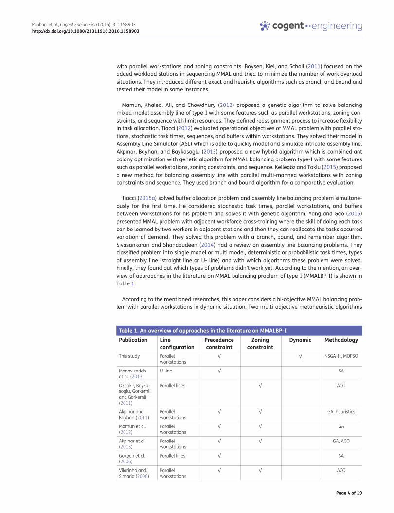
Tiacci (2015a) solved buffer allocation problem and assembly line balancing problem simultane-ously for the first time. He considered stochastic task times, parallel workstations, and buffers between workstations for his problem and solves it with genetic algorithm. Yang and Gao (2016) presented MMAL problem with adjacent workforce cross-training where the skill of doing each task can be learned by two workers in adjacent stations and then they can reallocate the tasks occurred variation of demand. They solved this problem with a branch, bound, and remember algorithm. Sivasankaran and Shahabudeen (2014) had a review on assembly line balancing problems. They classified problem into single model or multi model, deterministic or probabilistic task times, types of assembly line (straight line or U- line) and with which algorithms these problem were solved. Finally, they found out which types of problems didn’t work yet. According to the mention, an over-view of approaches in the literature on MMAL balancing problem of type-I (MMALBP-I) is shown in Table 1.

According to the mentioned researches, this paper considers a bi-objective MMAL balancing prob-lem with parallel workstations in dynamic situation. Two multi-objective metaheuristic algorithms

Table 1. An overview of approaches in the literature on MMALBP-IPublication Line

configurationPrecedence constraint

Zoning constraint

Dynamic Methodology

This study Parallel workstations

√ √ NSGA-II, MOPSO

Manavizadeh et al. (2013)

U-line √ SA

Ozbakir, Bayka-soglu, Gorkemli, and Gorkemli (2011)

Parallel lines √ ACO

Akpınar and Bayhan (2011)

Parallel workstations

√ √ GA, heuristics

Mamun et al. (2012)

Parallel workstations

√ √ GA

Akpınar et al. (2013)

Parallel workstations

√ √ GA, ACO

Gökҫen et al. (2006)

Parallel lines √ SA

Vilarinho and Simaria (2006)

Parallel workstations

√ √ ACO

Page 5 of 19

Rabbani et al., Cogent Engineering (2016), 3: 1158903http://dx.doi.org/10.1080/23311916.2016.1158903

are used to solve the problem. Finally, the performance of non-NSGA-II and multi-objective particle swarm optimization (MOPSO) algorithms is compared with each other for this problem. Details of this problem about objectives and assumptions are in the next section.

3. Problem descriptionIn this paper, we are trying to consider the layout of a MMAL including parallel workstations in dy-namic periods. Using parallel workstations has many features such as, two or more replicas of a workstation can perform the same set of tasks on different assemblies when required. Cycle times are allowed to be shorter than the longest task time in parallel workstations, thus it can increase the production rate and it provides better flexibility in designing the assembly line and the number of tasks performed by each worker increases (Vilarinho & Simaria, 2002).

Each work center (WC) comprises either one workstation for the instance of non-paralleling or multiple parallel workstations. A WC with multiple workstations is considered busy if every worksta-tions inside are busy. An example of parallel workstations is shown in Figure 1. According to this figure, one operator is assigned to each workstation. There are seven workstations in the mentioned figure where two of them are parallel with each other. These two parallel workstations have created one WC. Another five workstations that there are no parallel workstations with them consisted five WCs where each of workstation is one WC. In parallel workstations, the tasks assigned to the WC are not shared among the workstations, while every workstation can perform each one of the tasks (Tiacci, 2015b).

In such a way, workstations are replicated only when processing time of a task is higher than the cycle time for at least one model, so the number of this replication does not exceeded by the tasks which have a task time higher than the cycle time (Akpınar & Bayhan, 2011; Vilarinho & Simaria, 2002). According to the literature, this research has following objectives.

3.1. ObjectivesIn this research, there are two objectives which should be achieved: First of them is minimizing num-ber of workstations (Akpınar & Bayhan, 2011; Manavizadeh et al., 2013; Vilarinho & Simaria, 2002) and the second one is to maximize workload smoothness between workstations (Akpınar & Bayhan, 2011; Mamun et al., 2012; Vilarinho & Simaria, 2002, 2006). The second objective aims to balance the line and it means that for each model, the idle time is divided through the workstations equally (Mamun et al., 2012; Vilarinho & Simaria, 2006).

3.2. AssumptionsThe common assumptions of the problem are listed below:

• Assembly line balancing problem type-I are used.

• Precedence constraints and precedence diagrams for each product are known. Precedence con-straints indicate that an assignment should be allocated to a workstation, if it has no

Figure 1. An assembly line with parallel workstations.

Page 6 of 19

Rabbani et al., Cogent Engineering (2016), 3: 1158903http://dx.doi.org/10.1080/23311916.2016.1158903

predecessors, or if all of its predecessors have already been assigned to that workstation or its previous workstations.

• Task performance’s times of each product are known.

• Operators who are working in each workstation of the each line are multi-skilled and can be as-signed to work at any station (flexible workers).

• Setup times between models are supposed as insignificant.

• All the operators are permanent and we do not have overtime periods.

• The number of workstations are variable.

• Cycle time is given and we have dynamic periods to determine all variables in different periods to achieve efficient solutions.

• We have a straight line with parallel workstations which can also be worked on each side of any line. Workstations along the line can be replicated to create parallel workstations.

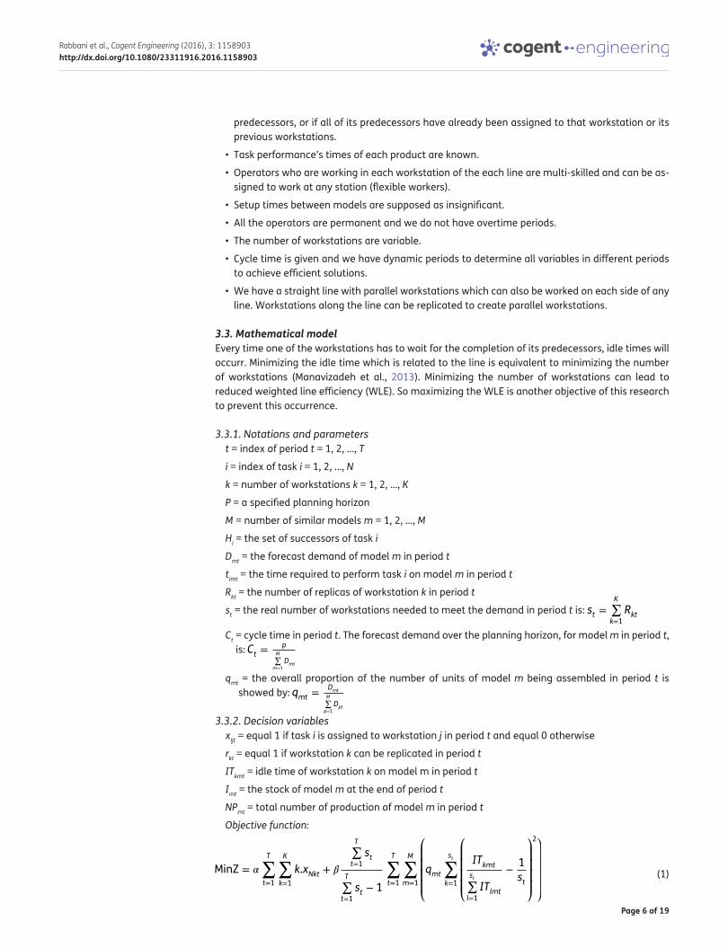
3.3. Mathematical modelEvery time one of the workstations has to wait for the completion of its predecessors, idle times will occurr. Minimizing the idle time which is related to the line is equivalent to minimizing the number of workstations (Manavizadeh et al., 2013). Minimizing the number of workstations can lead to reduced weighted line efficiency (WLE). So maximizing the WLE is another objective of this research to prevent this occurrence.

3.3.1. Notations and parameterst = index of period t = 1, 2, ..., T

i = index of task i = 1, 2, …, N

k = number of workstations k = 1, 2, …, K

P = a specified planning horizon

M = number of similar models m = 1, 2, …, M

Hi = the set of successors of task i

Dmt = the forecast demand of model m in period t

timt = the time required to perform task i on model m in period t

Rkt = the number of replicas of workstation k in period t

st = the real number of workstations needed to meet the demand in period t is: st =K∑k=1

Rkt

Ct  = cycle time in period t. The forecast demand over the planning horizon, for model m in period t, is: Ct =

pM∑m=1

Dmt

qmt   =  the overall proportion of the number of units of model m being assembled in period t is showed by: qmt =

DmtM∑p=1

Dpt

3.3.2. Decision variablesxijt = equal 1 if task i is assigned to workstation j in period t and equal 0 otherwise

rkt = equal 1 if workstation k can be replicated in period t

ITkmt = idle time of workstation k on model m in period t

Imt = the stock of model m at the end of period t

NPmt = total number of production of model m in period t

Objective function:

(1)MinZ = �

T�t=1

K�k=1

k.xNkt + �

T∑t=1

st

T∑t=1

st − 1

T�t=1

M�m=1

⎛⎜⎜⎜⎜⎝qmt

st�k=1

⎛⎜⎜⎜⎜⎝

ITkmtst∑l=1

ITlmt

−1

st

⎞⎟⎟⎟⎟⎠

2⎞⎟⎟⎟⎟⎠

Page 7 of 19

Rabbani et al., Cogent Engineering (2016), 3: 1158903http://dx.doi.org/10.1080/23311916.2016.1158903

The objective of minimizing the number of the workstations is represented by the first term in objective function, and the objective of smoothing workload between the workstations is the second term (Akpınar & Bayhan, 2011).

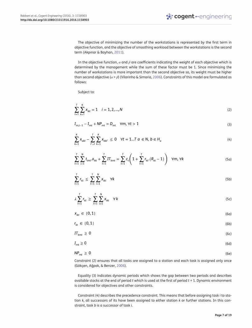
In the objective function, α and β are coefficients indicating the weight of each objective which is determined by the management while the sum of these factor must be 1. Since minimizing the number of workstations is more important than the second objective so, its weight must be higher than second objective (α ≻ β) (Vilarinho & Simaria, 2006). Constraints of this model are formulated as follows:

Subject to:

Constraint (2) ensures that all tasks are assigned to a station and each task is assigned only once (Gökҫen, Ağpak, & Benzer, 2006).

Equality (3) indicates dynamic periods which shows the gap between two periods and describes available stocks at the end of period t which is used at the first of period t + 1. Dynamic environment is considered for objectives and other constraints.

Constraint (4) describes the precedence constraint. This means that before assigning task i to sta-tion k, all successors of its have been assigned to either station k or further stations. In this con-straint, task b is a successor of task i.

(2)T∑t=1

K∑k=1

xikt = 1 i = 1, 2, ...,N

(3)Im,t−1 − Imt + NPmt = Dmt ∀m, ∀t > 1

(4)K∑k=1

xakt

−

T∑t�=t

K∑k=1

xbkt

� ≤ 0 ∀t = 1...T a ∈ N, b ∈ Ha

(5a)T∑t=1

N∑i=1

timt.xikt +

T∑t=1

ITkmt =

T∑t=1

ct

(1 +

T∑t=1

rkt.(Rkt − 1

))∀m, ∀k

(5b)T∑t=1

rkt ≤

T∑t=1

N∑i=1

xikt ∀k

(5c)�

T∑t=1

rkt ≥

T∑t=1

N∑i=1

xikt ∀ k

(6a)xikt ∈ {0, 1}

(6b)rkt ∈ {0, 1}

(6c)ITkmt ≥ 0

(6d)Imt ≥ 0

(6e)NPmt ≥ 0

Page 8 of 19

Rabbani et al., Cogent Engineering (2016), 3: 1158903http://dx.doi.org/10.1080/23311916.2016.1158903

Constraints (5a)–(5c) ensure that total time capacity of each workstation is up to task times assigned to each workstations and it will be equal to cycle time if there are no replication for that workstation. The maximum number of replicas of a workstation in a WC is up to the tasks which have a task time more than the cycle time for at least one model, and just the workstations where the time of the tasks assigned to it exceeds by the cycle time can be duplicated. In constraint (5c), λ is a very large positive integer (Akpınar & Bayhan, 2011).

Equalities (6a)–(6e) mean domain of the decision variables.

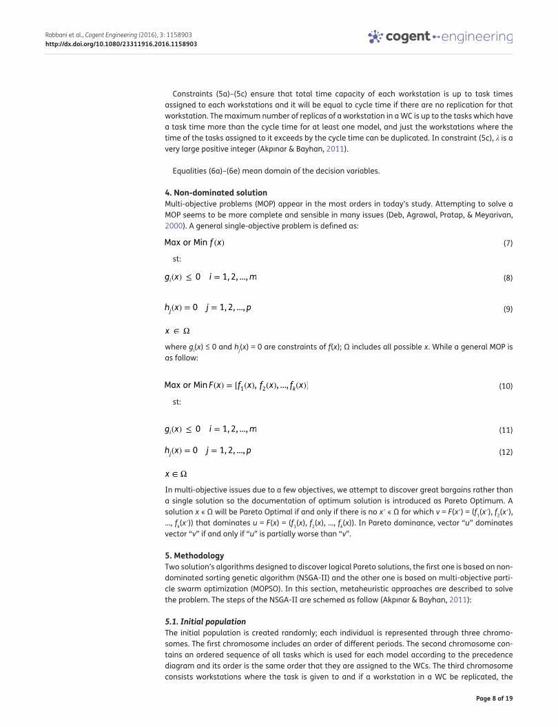
4. Non-dominated solutionMulti-objective problems (MOP) appear in the most orders in today’s study. Attempting to solve a MOP seems to be more complete and sensible in many issues (Deb, Agrawal, Pratap, & Meyarivan, 2000). A general single-objective problem is defined as:

st:

where gi(x) ≤ 0 and hj(x) = 0 are constraints of f(x); Ω includes all possible x. While a general MOP is as follow:

st:

In multi-objective issues due to a few objectives, we attempt to discover great bargains rather than a single solution so the documentation of optimum solution is introduced as Pareto Optimum. A solution x ∊ Ω will be Pareto Optimal if and only if there is no x′ ∊ Ω for which v = F(x′) = (f1(x′), f2(x′), ..., fk(x′)) that dominates u = F(x) = (f1(x), f2(x), ..., fk(x)). In Pareto dominance, vector “u” dominates vector “v” if and only if “u” is partially worse than “v”.

5. MethodologyTwo solution’s algorithms designed to discover logical Pareto solutions, the first one is based on non-dominated sorting genetic algorithm (NSGA-II) and the other one is based on multi-objective parti-cle swarm optimization (MOPSO). In this section, metaheuristic approaches are described to solve the problem. The steps of the NSGA-II are schemed as follow (Akpınar & Bayhan, 2011):

5.1. Initial populationThe initial population is created randomly; each individual is represented through three chromo-somes. The first chromosome includes an order of different periods. The second chromosome con-tains an ordered sequence of all tasks which is used for each model according to the precedence diagram and its order is the same order that they are assigned to the WCs. The third chromosome consists workstations where the task is given to and if a workstation in a WC be replicated, the

(7)Max or Min f (x)

(8)gi(x) ≤ 0 i = 1, 2, ...,m

(9)hj(x) = 0 j = 1, 2, ..., p

x ∈ Ω

(10)Max or Min F(x) = [f1(x), f

2(x), ..., fk(x)]

(11)gi(x) ≤ 0 i = 1, 2, ...,m

(12)hj(x) = 0 j = 1, 2, ..., p

x ∈ Ω

Page 9 of 19

Rabbani et al., Cogent Engineering (2016), 3: 1158903http://dx.doi.org/10.1080/23311916.2016.1158903

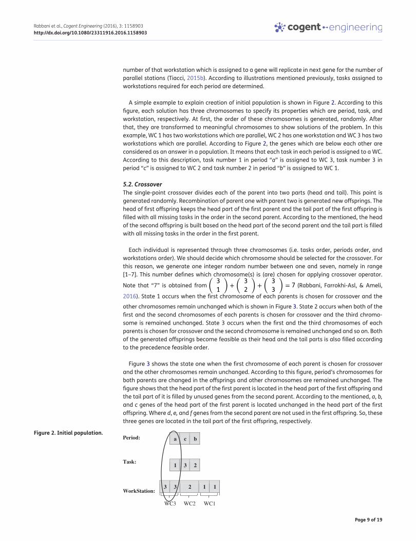
number of that workstation which is assigned to a gene will replicate in next gene for the number of parallel stations (Tiacci, 2015b). According to illustrations mentioned previously, tasks assigned to workstations required for each period are determined.

A simple example to explain creation of initial population is shown in Figure 2. According to this figure, each solution has three chromosomes to specify its properties which are period, task, and workstation, respectively. At first, the order of these chromosomes is generated, randomly. After that, they are transformed to meaningful chromosomes to show solutions of the problem. In this example, WC 1 has two workstations which are parallel, WC 2 has one workstation and WC 3 has two workstations which are parallel. According to Figure 2, the genes which are below each other are considered as an answer in a population. It means that each task in each period is assigned to a WC. According to this description, task number 1 in period “a” is assigned to WC 3, task number 3 in period “c” is assigned to WC 2 and task number 2 in period “b” is assigned to WC 1.

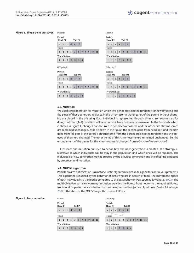
5.2. CrossoverThe single-point crossover divides each of the parent into two parts (head and tail). This point is generated randomly. Recombination of parent one with parent two is generated new offsprings. The head of first offspring keeps the head part of the first parent and the tail part of the first offspring is filled with all missing tasks in the order in the second parent. According to the mentioned, the head of the second offspring is built based on the head part of the second parent and the tail part is filled with all missing tasks in the order in the first parent.

Each individual is represented through three chromosomes (i.e. tasks order, periods order, and workstations order). We should decide which chromosome should be selected for the crossover. For this reason, we generate one integer random number between one and seven, namely in range [1–7]. This number defines which chromosome(s) is (are) chosen for applying crossover operator.

Note that “7” is obtained from (3

1

)+

(3

2

)+

(3

3

)= 7 (Rabbani, Farrokhi-Asl, & Ameli,

2016). State 1 occurs when the first chromosome of each parents is chosen for crossover and the

other chromosomes remain unchanged which is shown in Figure 3. State 2 occurs when both of the first and the second chromosomes of each parents is chosen for crossover and the third chromo-some is remained unchanged. State 3 occurs when the first and the third chromosomes of each parents is chosen for crossover and the second chromosome is remained unchanged and so on. Both of the generated offsprings become feasible as their head and the tail parts is also filled according to the precedence feasible order.

Figure 3 shows the state one when the first chromosome of each parent is chosen for crossover and the other chromosomes remain unchanged. According to this figure, period’s chromosomes for both parents are changed in the offsprings and other chromosomes are remained unchanged. The figure shows that the head part of the first parent is located in the head part of the first offspring and the tail part of it is filled by unused genes from the second parent. According to the mentioned, a, b, and c genes of the head part of the first parent is located unchanged in the head part of the first offspring. Where d, e, and f genes from the second parent are not used in the first offspring. So, these three genes are located in the tail part of the first offspring, respectively.

Figure 2. Initial population.Period: a c b

Task: 1 3 2

WorkStation:3 3 2 1 1

WC3 WC2 WC1

Page 10 of 19

Rabbani et al., Cogent Engineering (2016), 3: 1158903http://dx.doi.org/10.1080/23311916.2016.1158903

5.3. MutationWe used swap operation for mutation which two genes are selected randomly for new offspring and the place of these genes are replaced in the chromosome. Other genes of the parent without chang-ing are placed in the offspring. Each individual is represented through three chromosomes, so for doing mutation [1–7] condition will be occur which are as same as crossover. In the first state which is shown in Figure 4, changes are occurred in period chromosome and the other two chromosomes are remained unchanged. As it is shown in the figure, the second gene from head part and the fifth gene from tail part of the period’s chromosome from the parent are selected randomly and the pal-aces of them are changed. The other genes of this chromosome are remained unchanged. So, the arrangement of the genes for this chromosome is changed from a-b-c-d-e-f to a-e-c-d-b-f.

Crossover and mutation are used to define how the next generation is created. The strategy il-lustrative of which individuals will be stay in the population and which ones will be replaced. The individuals of new generation may be created by the previous generation and the offspring produced by crossover and mutation.

5.4. MOPSO algorithmParticle swarm optimization is a metaheuristic algorithm which is designed for continuous problems. This algorithm is inspired by the behavior of birds who are in search of food. The movement’ speed of each individual into the food is compared to the best behavior (Parsopoulos & Vrahatis, 2002). The multi-objective particle swarm optimization provides the Pareto front nearer to the required Pareto fronts and its performance is better than some other multi-objective algorithms (Coello & Lechuga, 2002). The steps of the MOPSO algorithm are as follows:

Figure 3. Single-point crossover. Parent1: Parent2:

Period: Head P1 Tail P1

a b c d e f

Period:Head P2 Tail P2

a c d e b fTask:

1 2 4 5 3 6 7 8 9 10 11

Task:

1 6 7 8 9 2 4 5 3 10 11

WorkStation:

1 1 2 2 3 3 4

WorkStation:

1 1 3 3 4 2 2

Offspring1: Offspring2:

Period: Head O1 Tail O1

a b c d e f

Period: Head O2 Tail O2

a c d b e f

Task:

1 2 4 5 3 6 7 8 9 10 11

Task:

1 6 7 8 9 2 4 5 3 10 11

WorkStation:

1 1 2 2 3 3 4

WorkStation:

1 1 3 3 4 2 2 1

Figure 4. Swap mutation. Parent: Offspring:

Period: Head P Tail P

a b c d e f

Period: Head O Tail O

a e c d b f

Task:

1 2 4 5 3 6 7 8 9 10 11

Task:

1 2 4 5 3 6 7 8 9 10 11

WorkStation:

1 1 2 2 3 3 4

WorkStation:

1 1 2 2 3 3 4

Page 11 of 19

Rabbani et al., Cogent Engineering (2016), 3: 1158903http://dx.doi.org/10.1080/23311916.2016.1158903

Step 1: Generate the initial population of particles.

Step 2: Each particle’ velocity is generated and saved in the velocity vector which determines the direction in which a particle should move to improve its new position.

Step 3: The new position of each particle is saved as memory of particle in the personal best, which shows the best position of each individual. The new position of each particle is calculated by sum of its previous position and its velocity vector. If the new position calculated for each particle is better than its previous position, the personal best should be equal to that position. The previous position in the memory should be kept when the new position is dominated by its.

Step 4: Leaders which is the position of non-dominated particles is saved in an external memory called global best. Leaders lead other particles towards better areas in search space and considered for all the individual.

Step 5: Until the number of iteration is same as the maximum number of iterations, we should re-peat step 4.

6. Numerical resultsThe performance of the NSGA-II and MOPSO algorithms is investigated and the related results are analyzed. The algorithms are coded in MATLAB R2013b and run on Intel CORE i7 2.30 GHz on per-sonal computer with 6 GB RAM.

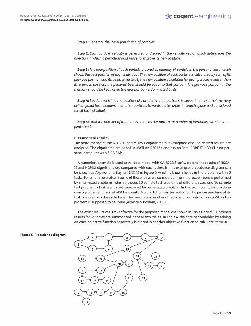
A numerical example is used to validate model with GAMS 23.5 software and the results of NSGA-II and MOPSO algorithms are compared with each other. In this example, precedence diagram can be shown as Akpınar and Bayhan (2011) in Figure 5 which is known for us in the problem with 30 tasks. For small size problem some of these tasks are considered. The initial experiment is performed by small-sized problems, which includes 10 sample test problems of different sizes, and 10 sample test problems of different sizes were used for large-sized problem. In this example, tasks are done over a planning horizon of 400 time units. A workstation can be replicated if a processing time of its task is more than the cycle time. The maximium number of replicas of workstations in a WC in this problem is supposed to be three (Akpınar & Bayhan, 2011).

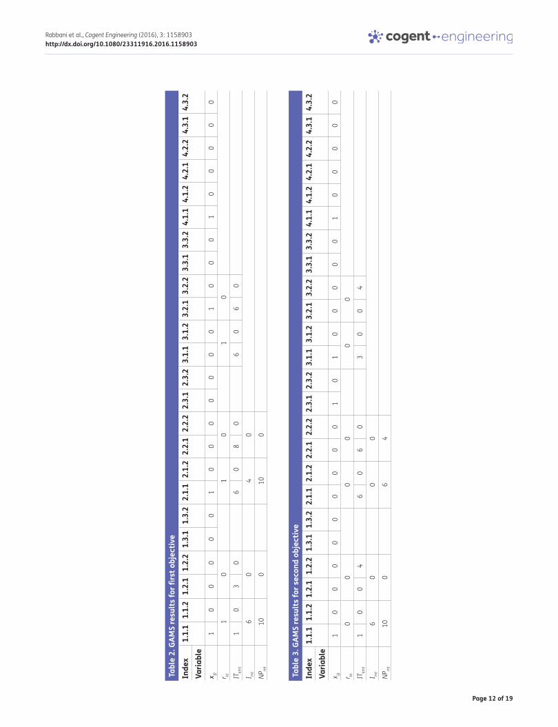
The exact results of GAMS software for the proposed model are shown in Tables 2 and 3. Obtained results for variables are summarized in these two tables. In Table 4, the obtained variables by solving an each objective function separately is placed in another objective function to calculate its value.

Figure 5. Precedence diagram.

Page 12 of 19

Rabbani et al., Cogent Engineering (2016), 3: 1158903http://dx.doi.org/10.1080/23311916.2016.1158903

Tabl

e 3.

GAM

S re

sults

for s

econ

d ob

ject

ive

Inde

x1.

1.1

1.1.

21.

2.1

1.2.

21.

3.1

1.3.

22.

1.1

2.1.

22.

2.1

2.2.

22.

3.1

2.3.

23.

1.1

3.1.

23.

2.1

3.2.

23.

3.1

3.3.

24.

1.1

4.1.

24.

2.1

4.2.

24.

3.1

4.3.

2Va

riabl

ex ijt

10

00

00

00

00

10

10

00

00

10

00

00

r kt0

00

00

0

ITkm

t1

00

46

06

03

00

4

I mt

60

00

NPm

t10

06

4

Tabl

e 2.

GAM

S re

sults

for fi

rst o

bjec

tive

Inde

x1.

1.1

1.1.

21.

2.1

1.2.

21.

3.1

1.3.

22.

1.1

2.1.

22.

2.1

2.2.

22.

3.1

2.3.

23.

1.1

3.1.

23.

2.1

3.2.

23.

3.1

3.3.

24.

1.1

4.1.

24.

2.1

4.2.

24.

3.1

4.3.

2Va

riabl

ex ijt

10

00

00

10

00

00

00

10

00

10

00

00

r kt1

01

01

0

ITkm

t1

03

06

08

06

06

0

I mt

60

40

NPm

t10

010

0

Page 13 of 19

Rabbani et al., Cogent Engineering (2016), 3: 1158903http://dx.doi.org/10.1080/23311916.2016.1158903

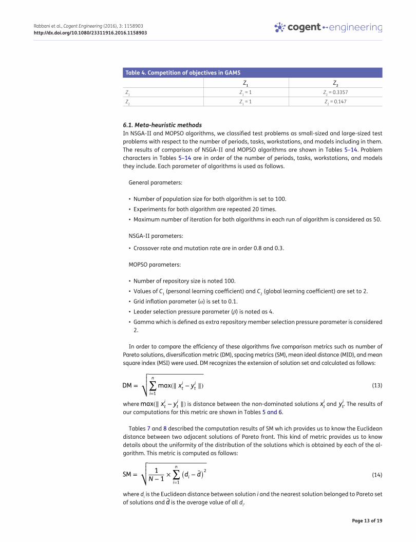
6.1. Meta-heuristic methodsIn NSGA-II and MOPSO algorithms, we classified test problems as small-sized and large-sized test problems with respect to the number of periods, tasks, workstations, and models including in them. The results of comparison of NSGA-II and MOPSO algorithms are shown in Tables 5–14. Problem characters in Tables 5–14 are in order of the number of periods, tasks, workstations, and models they include. Each parameter of algorithms is used as follows.

General parameters:

• Number of population size for both algorithm is set to 100.

• Experiments for both algorithm are repeated 20 times.

• Maximum number of iteration for both algorithms in each run of algorithm is considered as 50.

NSGA-II parameters:

• Crossover rate and mutation rate are in order 0.8 and 0.3.

MOPSO parameters:

• Number of repository size is noted 100.

• Values of C1 (personal learning coefficient) and C2 (global learning coefficient) are set to 2.

• Grid inflation parameter (α) is set to 0.1.

• Leader selection pressure parameter (β) is noted as 4.

• Gamma which is defined as extra repository member selection pressure parameter is considered 2.

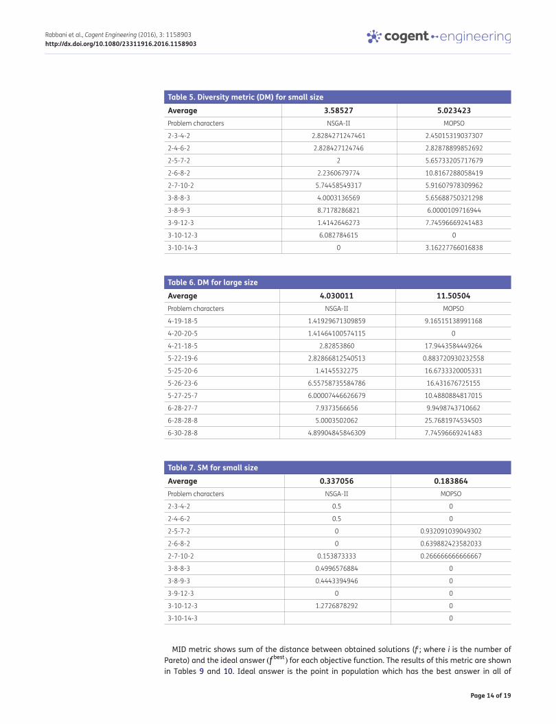
In order to compare the efficiency of these algorithms five comparison metrics such as number of Pareto solutions, diversification metric (DM), spacing metrics (SM), mean ideal distance (MID), and mean square index (MSI) were used. DM recognizes the extension of solution set and calculated as follows:

where max(∥ xit − yit ∥) is distance between the non-dominated solutions xit and yit. The results of

our computations for this metric are shown in Tables 5 and 6.

Tables 7 and 8 described the computation results of SM wh ich provides us to know the Euclidean distance between two adjacent solutions of Pareto front. This kind of metric provides us to know details about the uniformity of the distribution of the solutions which is obtained by each of the al-gorithm. This metric is computed as follows:

where di is the Euclidean distance between solution i and the nearest solution belonged to Pareto set of solutions and d̄ is the average value of all di.

(13)DM =

√√√√ n∑i=1

max(∥ xit − yit ∥)

(14)SM =

√√√√ 1

N − 1×

n∑i=1

(di − d̄

)2

Table 4. Competition of objectives in GAMSZ1 Z2

Z1 Z1 = 1 Z2 = 0.3357

Z2 Z1 = 1 Z2 = 0.147

Page 14 of 19

Rabbani et al., Cogent Engineering (2016), 3: 1158903http://dx.doi.org/10.1080/23311916.2016.1158903

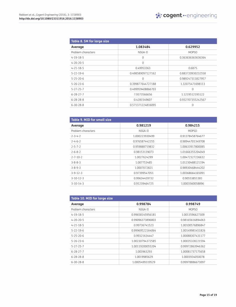
MID metric shows sum of the distance between obtained solutions (fi ; where i is the number of Pareto) and the ideal answer (f best) for each objective function. The results of this metric are shown in Tables 9 and 10. Ideal answer is the point in population which has the best answer in all of

Table 5. Diversity metric (DM) for small sizeAverage 3.58527 5.023423Problem characters NSGA-II MOPSO

2-3-4-2 2.8284271247461 2.45015319037307

2-4-6-2 2.828427124746 2.82878899852692

2-5-7-2 2 5.65733205717679

2-6-8-2 2.2360679774 10.8167288058419

2-7-10-2 5.74458549317 5.91607978309962

3-8-8-3 4.0003136569 5.65688750321298

3-8-9-3 8.7178286821 6.0000109716944

3-9-12-3 1.4142646273 7.74596669241483

3-10-12-3 6.082784615 0

3-10-14-3 0 3.16227766016838

Table 6. DM for large sizeAverage 4.030011 11.50504Problem characters NSGA-II MOPSO

4-19-18-5 1.41929671309859 9.16515138991168

4-20-20-5 1.41464100574115 0

4-21-18-5 2.82853860 17.9443584449264

5-22-19-6 2.82866812540513 0.883720930232558

5-25-20-6 1.4145532275 16.6733320005331

5-26-23-6 6.55758735584786 16.431676725155

5-27-25-7 6.00007446626679 10.4880884817015

6-28-27-7 7.9373566656 9.9498743710662

6-28-28-8 5.0003502062 25.7681974534503

6-30-28-8 4.89904845846309 7.74596669241483

Table 7. SM for small sizeAverage 0.337056 0.183864Problem characters NSGA-II MOPSO

2-3-4-2 0.5 0

2-4-6-2 0.5 0

2-5-7-2 0 0.932091039049302

2-6-8-2 0 0.639882423582033

2-7-10-2 0.153873333 0.266666666666667

3-8-8-3 0.4996576884 0

3-8-9-3 0.4443394946 0

3-9-12-3 0 0

3-10-12-3 1.2726878292 0

3-10-14-3 0

Page 15 of 19

Rabbani et al., Cogent Engineering (2016), 3: 1158903http://dx.doi.org/10.1080/23311916.2016.1158903

Table 8. SM for large sizeAverage 1.083484 0.629952Problem characters NSGA-II MOPSO

4-19-18-5 0 0.363636363636364

4-20-20-5 0

4-21-18-5 0.49953363 0.6875

5-22-19-6 0.498589097127162 0.883720930232558

5-25-20-6 0 0.989247311827957

5-26-23-6 0.399877644727188 1.32075471698113

5-27-25-7 0.499959408866703 0

6-28-27-7 7.9373566656 1.1219512195122

6-28-28-8 0.4281549607 0.932707355242567

6-30-28-8 0.571371224816095 0

Table 9. MID for small sizeAverage 0.981219 0.984215Problem characters NSGA-II MOPSO

2-3-4-2 1.000223930499 0.91378458764677

2-4-6-2 0.976587442255 0.98944701349708

2-5-7-2 0.959888719832 1.00633917800085

2-6-8-2 0.98153139073 1.01666355204049

2-7-10-2 1.0027624299 1.00472327236632

3-8-8-3 1.007753485 1.01230488121194

3-8-9-3 1.0007072821 0.98930468444202

3-9-12-3 0.97399547051 1.00368664165091

3-10-12-3 0.99634459732 0.90553851381

3-10-14-3 0.91239464725 1.0003560058896

Table 10. MID for large sizeAverage 0.998784 0.998749Problem characters NSGA-II MOPSO

4-19-18-5 0.99658145956181 1.0013596627309

4-20-20-5 0.99096373896803 0.98165616894063

4-21-18-5 0.99736741523 1.00100576896847

5-22-19-6 0.99969522164064 1.00149981451826

5-25-20-6 0.99321634447 1.00088307431177

5-26-23-6 1.00230794372585 1.00035328221594

5-27-25-7 1.00119200055204 0.99972863946362

6-28-27-7 1.003963293 1.00081737175658

6-28-28-8 1.0019985629 1.0003934050078

6-30-28-8 1.0005499319529 0.99978886673097

Page 16 of 19

Rabbani et al., Cogent Engineering (2016), 3: 1158903http://dx.doi.org/10.1080/23311916.2016.1158903

Table 11. MSI for small sizeAverage 0.02849 0.061832Problem characters NSGA-II MOPSO

2-3-4-2 1.11022302462516e-16 0.0987654320987654

2-4-6-2 1.80411241501588e-16 0.0904977375565611

2-5-7-2 5.55111512312578e-17 0.176470588235294

2-6-8-2 1.11022302462516e-16 0.126315789473684

2-7-10-2 0.0391304347826 2.775557561562e-16

3-8-8-3 0.114942528735 0.0775862068965516

3-8-9-3 0.0732758620689 0.0486815415821498

3-9-12-3 0.012018381053 4.440892098500e-16

3-10-12-3 0.045528455284 0

3-10-14-3 0 1.110223024625e-16

Table 12. MSI for large sizeAverage 0.068898 6.72e-16Problem characters NSGA-II MOPSO

4-19-18-5 0.120229042105453 5.55111512312578e-16

4-20-20-5 0.034778450949676 0

4-21-18-5 0.0430062498 4.9960036108132e-16

5-22-19-6 0.0639204545454549 6.10622663543836e-16

5-25-20-6 0.03100103762 3.88578058618805e-16

5-26-23-6 0.0886902165524723 3.33066907387547e-16

5-27-25-7 0.059846154767623 2.77555756156289e-16

6-28-27-7 0.1508811481 1.77635683940025e-15

6-28-28-8 0.0519081911 8.32667268468867e-16

6-30-28-8 0.044718805316506 1.4432899320127e-15

Table 13. Number of Pareto solutions and computational time for small sizeNPS Computational time(s)

Average 3 2.9 74.41495 9.71821Problem characters NSGA-II MOPSO NSGA-II MOPSO

2-3-4-2 3 2 44.71 3.304637

2-4-6-2 3 2 48.195905 3.930728

2-5-7-2 2 4 46.378222 4.814735

2-6-8-2 3 6 56.205583 5.498103

2-7-10-2 4 4 57.127584 5.665040

3-8-8-3 3 2 85.788409 12.088588

3-8-9-3 5 2 94.436604 14.718414

3-9-12-3 2 4 94.434902 14.325840

3-10-12-3 4 1 110.221109 14.119085

3-10-14-3 1 2 106.651202 18.716929

Page 17 of 19

Rabbani et al., Cogent Engineering (2016), 3: 1158903http://dx.doi.org/10.1080/23311916.2016.1158903

objective functions in the problem. The ideal answer in this problem is considered as the point of (0,0) because all objectives should be minimized. fmax

1,total is the maximum value of the first objective

function and fmin1,total

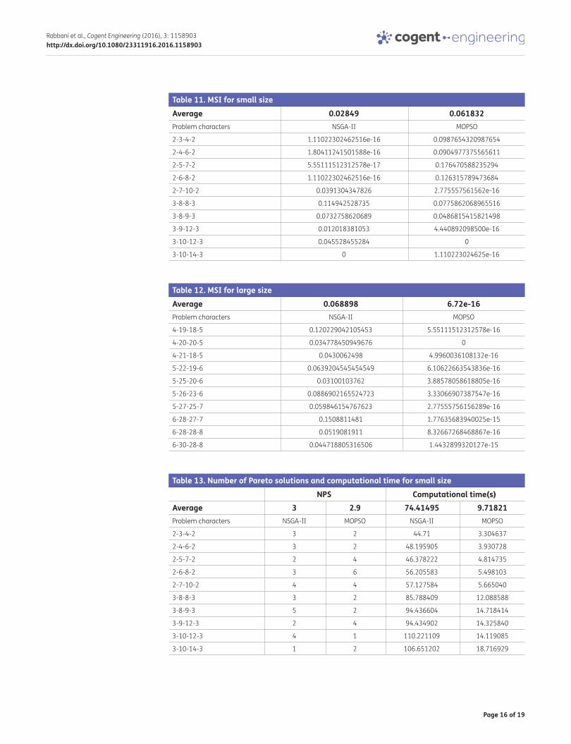
is the minimum value of it. It is better to have less value of this metric. This metric is computed as follows:

MSI which is shown in Tables 11 and 12 is the mean square of the maximum value of objective func-tion minus the minimum value of the objective function.

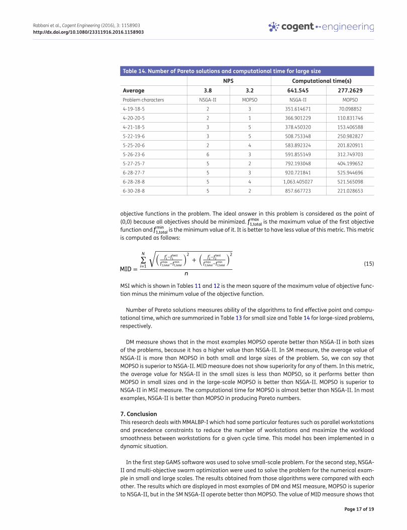
Number of Pareto solutions measures ability of the algorithms to find effective point and compu-tational time, which are summarized in Table 13 for small size and Table 14 for large-sized problems, respectively.

DM measure shows that in the most examples MOPSO operate better than NSGA-II in both sizes of the problems, because it has a higher value than NSGA-II. In SM measure, the average value of NSGA-II is more than MOPSO in both small and large sizes of the problem. So, we can say that MOPSO is superior to NSGA-II. MID measure does not show superiority for any of them. In this metric, the average value for NSGA-II in the small sizes is less than MOPSO, so it performs better than MOPSO in small sizes and in the large-scale MOPSO is better than NSGA-II. MOPSO is superior to NSGA-II in MSI measure. The computational time for MOPSO is almost better than NSGA-II. In most examples, NSGA-II is better than MOPSO in producing Pareto numbers.

7. ConclusionThis research deals with MMALBP-I which had some particular features such as parallel workstations and precedence constraints to reduce the number of workstations and maximize the workload smoothness between workstations for a given cycle time. This model has been implemented in a dynamic situation.

In the first step GAMS software was used to solve small-scale problem. For the second step, NSGA-II and multi-objective swarm optimization were used to solve the problem for the numerical exam-ple in small and large scales. The results obtained from those algorithms were compared with each other. The results which are displayed in most examples of DM and MSI measure, MOPSO is superior to NSGA-II, but in the SM NSGA-II operate better than MOPSO. The value of MID measure shows that

(15)MID =

N∑i=1

��f i1−f best

1

fmax1,total

−fmin1,total

�2+

�f i2−f best

2

fmax2,total

−fmin2,total

�2

n

Table 14. Number of Pareto solutions and computational time for large sizeNPS Computational time(s)

Average 3.8 3.2 641.545 277.2629Problem characters NSGA-II MOPSO NSGA-II MOPSO

4-19-18-5 2 3 351.614671 70.098852

4-20-20-5 2 1 366.901229 110.831746

4-21-18-5 3 5 378.450320 153.406588

5-22-19-6 3 5 508.753348 250.982827

5-25-20-6 2 4 583.892324 201.820911

5-26-23-6 6 3 591.855149 312.749703

5-27-25-7 5 2 792.193048 404.199652

6-28-27-7 5 3 920.721841 525.944696

6-28-28-8 5 4 1,063.405027 521.565098

6-30-28-8 5 2 857.667723 221.028653

Page 18 of 19

Rabbani et al., Cogent Engineering (2016), 3: 1158903http://dx.doi.org/10.1080/23311916.2016.1158903

in small scale, NSGA-II is better than MOPSO; and in large scale MOPSO is better than NSGA-II, so this measure doesn’t show superiority for any of them. The computational time for MOPSO is almost bet-ter than NSGA-II, but in most examples NSGA-II is better than MOPSO in producing Pareto numbers.

For future research, MMAL balancing problem of type-II with U- line can be used in a dynamic situ-ation when cycle time is unknown and number of workstations is known using the constraints of number of operators and skill level of them.

FundingThe authors received no direct funding for this research.

Author detailsMasoud Rabbani1

E-mail: [email protected] Siadatian1

E-mail: [email protected] Farrokhi-Asl2

E-mail: [email protected] Manavizadeh3

E-mail: [email protected] School of Industrial Engineering, College of Engineering,

University of Tehran, P.O. Box 11155-4563 Tehran, Iran.2 School of Industrial Engineering, Iran University of Science &

Technology, Tehran, Iran.3 Department of Industrial Engineering, KHATAM University,

Tehran, Iran.

Citation informationCite this article as: Multi-objective optimization algorithms for mixed model assembly line balancing problem with parallel workstations, Masoud Rabbani, Reyhaneh Siadatian, Hamed Farrokhi-Asl & Neda Manavizadeh, Cogent Engineering (2016), 3: 1158903.

Cover imageSource: Authors.

ReferencesAkpınar, S., & Bayhan, G. M. (2011). A hybrid genetic algorithm

for mixed model assembly line balancing problem with parallel workstations and zoning constraints. Engineering Applications of Artificial Intelligence, 24, 449–457. http://dx.doi.org/10.1016/j.engappai.2010.08.006

Akpınar, S., Bayhan, G. M., & Baykasoglu, A. (2013). Hybridizing ant colony optimization via genetic algorithm for mixed-model assembly line balancing problem with sequence dependent setup times between tasks. Applied Soft Computing, 13, 574–589. http://dx.doi.org/10.1016/j.asoc.2012.07.024

Boysen, N., Fliedner, M., & Scholl, A. (2007). A classification of assembly line balancing problems. European Journal of Operational Research, 183, 674–693. http://dx.doi.org/10.1016/j.ejor.2006.10.010

Boysen, N., Fliedner, M., & Scholl, A. (2009). Sequencing mixed-model assembly lines: Survey, classification and model critique. European Journal of Operational Research, 192, 349–373. http://dx.doi.org/10.1016/j.ejor.2007.09.013

Boysen, N., Kiel, M., & Scholl, A. (2011). Sequencing mixed-model assembly lines to minimise the number of work overload situations. International Journal of Production Research, 16, 4735–4760. http://dx.doi.org/10.1080/00207543.2010.507607

Coello, C. A., & Lechuga, M. S. (2002). MOPSO: A proposal for multiple objective particle swarm optimization. Proceedings of the IEEE Congress on Evolutionary Computation, 2, 1051–1056.

Deb, K., Agrawal, S., Pratap, A., & Meyarivan, T. (2000). A fast elitist non-dominated sorting genetic algorithm for multi-objective optimization: NSGA-II. Lecture notes in computer science, 1917, 849–858. http://dx.doi.org/10.1007/3-540-45356-3

Gökҫen, H., Ağpak, K., & Benzer, R. (2006). Balancing of parallel assembly lines. International Journal of Production Economics, 103, 600–609.

Hamzadayi, A., & Yildiz, G. (2012). A genetic algorithm based approach for simultaneously balancing and sequencing of mixed-model U-lines with parallel workstations and zoning constraints. Computers & Industrial Engineering, 62, 206–215.

Kellegöz, T., & Toklu, B. (2015). A priority rule-based constructive heuristic and an improvement method for balancing assembly lines with parallel multi-manned workstations. International Journal of Production Research, 53, 736–756. http://dx.doi.org/10.1080/00207543.2014.920548

Mamun, A. A., Khaled, A. A., Ali, S. M., & Chowdhury, M. M. (2012). A heuristic approach for balancing mixed-model assembly line of type I using genetic algorithm. International Journal of Production Research, 50, 5106–5116. http://dx.doi.org/10.1080/00207543.2011.643830

Manavizadeh, N., Hosseini, N. S., Rabbani, M., & Jolai, F. (2013). A simulated annealing algorithm for a mixed model assembly U-line balancing type-I problem considering human efficiency and Just-In-Time approach. Computers & Industrial Engineering, 64, 669–685.

McMullen, P. R., & Frazier, G. V. (1998). Using simulated annealing to solve a multiobjective assembly line balancing problem with parallel workstations. International Journal of Production Research, 36, 2717–2741. http://dx.doi.org/10.1080/002075498192454

McMullen, P. R., & Tarasewich, P. (2003). Using ant techniques to solve the assembly line balancing problem. IIE Transactions, 35, 605–617. http://dx.doi.org/10.1080/07408170304354

Ozbakir, L., Baykasoglu, A., Gorkemli, B., & Gorkemli, L. (2011). Multiple-colony ant algorithm for parallel assembly line balancing problem. Applied Soft Computing, 11, 3186–3198. http://dx.doi.org/10.1016/j.asoc.2010.12.021

Parsopoulos, K. E., & Vrahatis, M. N. (2002). Particle swarm optimization method in multiobjective problems. In Proceedings of the 2002 ACM Symposium on Applied Computing, ACM (pp. 603–607). Madrid. http://dx.doi.org/10.1145/508791

Rabbani, M., Farrokhi-Asl, H., & Ameli, M. (2016). Solving a fuzzy multi-objective products and time planning using hybrid meta-heuristic algorithm: Gas refinery case study. Uncertain Supply Chain Management, 4, 93–106. http://dx.doi.org/10.5267/j.uscm.2015.12.002

Rabbani, M., Kazemi, S. M., & Manavizadeh, N. (2012). Mixed model U-line balancing type-1 problem: A new approach. Journal of Manufacturing Systems, 31, 131–138. http://dx.doi.org/10.1016/j.jmsy.2012.02.002

Simaria, A. S., & Vilarinho, P. M. (2004). A genetic algorithm based approach to the mixed- model assembly line

Page 19 of 19

Rabbani et al., Cogent Engineering (2016), 3: 1158903http://dx.doi.org/10.1080/23311916.2016.1158903

© 2016 The Author(s). This open access article is distributed under a Creative Commons Attribution (CC-BY) 4.0 license.You are free to: Share — copy and redistribute the material in any medium or format Adapt — remix, transform, and build upon the material for any purpose, even commercially.The licensor cannot revoke these freedoms as long as you follow the license terms.

Under the following terms:Attribution — You must give appropriate credit, provide a link to the license, and indicate if changes were made. You may do so in any reasonable manner, but not in any way that suggests the licensor endorses you or your use. No additional restrictions You may not apply legal terms or technological measures that legally restrict others from doing anything the license permits.

Cogent Engineering (ISSN: 2331-1916) is published by Cogent OA, part of Taylor & Francis Group. Publishing with Cogent OA ensures:• Immediate, universal access to your article on publication• High visibility and discoverability via the Cogent OA website as well as Taylor & Francis Online• Download and citation statistics for your article• Rapid online publication• Input from, and dialog with, expert editors and editorial boards• Retention of full copyright of your article• Guaranteed legacy preservation of your article• Discounts and waivers for authors in developing regionsSubmit your manuscript to a Cogent OA journal at www.CogentOA.com

balancing problem of type II. Computers & Industrial Engineering, 47, 391–407.

Simaria, A. S., & Vilarinho, P. M. (2009). 2-ANTBAL: An ant colony optimization algorithm for balancing two-sided assembly lines. Computers & Industrial Engineering, 56, 489–506.

Soman, C. A., van Donk, D. P., & Gaalman, G. (2004). Combined make-to-order and make-to-stock in a food production system. International Journal of Production Economics, 90, 223–235. http://dx.doi.org/10.1016/S0925-5273(02)00376-6

Sivasankaran, P., & Shahabudeen, P. (2014). Literature review of assembly line balancing problems. The International Journal of Advanced Manufacturing Technology, 73, 1665–1694. http://dx.doi.org/10.1007/s00170-014-5944-y

Tiacci, L. (2012). Event and object oriented simulation to fast evaluate operational objectives of mixed model assembly lines problems. Simulation Modelling Practice and Theory, 24, 35–48. http://dx.doi.org/10.1016/j.simpat.2012.01.004

Tiacci, L. (2015a). Simultaneous balancing and buffer allocation decisions for the design of mixed-model assembly lines with parallel workstations and stochastic

task times. International Journal of Production Economics, 162, 201–215. http://dx.doi.org/10.1016/j.ijpe.2015.01.022

Tiacci, L. (2015b). Coupling a genetic algorithm approach and a discrete event simulator to design mixed-model un-paced assembly lines with parallel workstations and stochastic task times. International Journal of Production Economics, 159, 319–333. http://dx.doi.org/10.1016/j.ijpe.2014.05.005

Vilarinho, P. M., & Simaria, A. S. (2002). A two-stage heuristic method for balancing mixed-model assembly lines with parallel workstations. International Journal of Production Research, 40, 1405–1420. http://dx.doi.org/10.1080/00207540110116273

Vilarinho, P. M., & Simaria, A. S. (2006). ANTBAL: An ant colony optimization algorithm for balancing mixed-model assembly lines with parallel workstations. International Journal of Production Research, 44, 291–303. http://dx.doi.org/10.1080/00207540500227612

Yang, C., & Gao, J. (2016). Balancing mixed-model assembly lines using adjacent cross-training in a demand variation environment. Computers & Operations Research, 65, 139–148.