MIXED ZERO-ONE LINEAR PROGRAMS UNDER OBJECTIVE ...

MIXED ZERO-ONE LINEAR PROGRAMS UNDER OBJECTIVEUNCERTAINTY: A COMPLETELY POSITIVE REPRESENTATION

Karthik Natarajan1 · Chung Piaw Teo2 · Zhichao Zheng3

Abstract. In this paper, we analyze mixed 0-1 linear programs under objective uncer-tainty. The mean vector and the second moment matrix of the nonnegative objectivecoefficients is assumed to be known, but the exact form of the distribution is unknown.Our main result shows that computing a tight upper bound on the expected value of amixed 0-1 linear program in maximization form with random objective is a completelypositive program. This naturally leads to semidefinite programming relaxations that aresolvable in polynomial time but provide weaker bounds. The result can be extended todeal with uncertainty in the moments and more complicated objective functions. Exam-ples from order statistics and project networks highlight the applications of the model.Our belief is that the model will open an interesting direction for future research in discreteand linear optimization under uncertainty.

Keywords. Mixed 0-1 linear program; Moments; Completely positive program

1. Introduction

One of the fundamental problems in mixed 0-1 linear programs under uncertainty is tocompute the expected optimal objective value. Consider the random optimization problem,

(1.1)

Z(c) = max cT x

s.t. aTi x = bi ∀i = 1, . . . , m

x ≥ 0

xj ∈ 0, 1 ∀j ∈ B ⊆ 1, . . . , nwhere x ∈ Rn

+ is the decision vector and c is the random objective coefficient vector. Thesubset B ⊆ 1, . . . , n indexes the 0-1 decision variables and 1, . . . , n \B indexes thecontinuous decision variables. Problem (1.1) includes the class of 0-1 integer programs andthe class of linear programs as special cases. Given distributional information on c, theobject of interest is the expected optimal value E[Z(c)].

1Department of Management Sciences, City University of Hong Kong, Hong Kong. Email:[email protected]. Part of this work was supported by the NUS Academic Research Fund R-146-000-112-112.2Department of Decision Sciences, NUS Business School, National University of Singapore, Singapore117591. Email: [email protected] of Decision Sciences, NUS Business School, National University of Singapore, Singapore117591. Email: [email protected]. Part of this work was done when the author was at the Departmentof Mathematics, Faculty of Science, National University of Singapore.

1

Page 2 of 36

This problem has been extensively studied in network reliability applications. Networkreliability deals with the design and analysis of networks that are subject to random vari-ation in the components. Such network applications arise in, for example, telecommu-nication, transportation and power systems. The random weights c on the edges in thenetwork represent random lengths, capacities or durations. For designated source node s

and destination node t, popular reliability measures include the shortest s− t path length,the longest s − t path length in a directed acyclic graph and the maximum s − t flow.The goal is to compute properties of the network reliability measure such as the averagevalue or the probability distribution of Z(c). For an excellent review on applications andalgorithms for the network reliability analysis problem, the reader is referred to Ball et al.[2] and the references therein. Under the assumption of independence among the randomweights, Hagstrom [18] showed that computing the expected value of the longest path in adirected acyclic graph is #P-complete, when the arc lengths are restricted to taking twopossible values each. The expected longest path is not computable in time polynomial inthe size of the input unless P = NP . The #P-hardness results for other network reliabil-ity measures are discussed in Valiant [40] and Provan and Ball [37]. Methods developedinclude identification of efficient algorithms for special cases, enumerative methods, bound-ing methods and Monte Carlo methods. For the shortest path problem with exponentiallydistributed arc lengths, Kulkarni [23] developed a Markov chain based method to computethe expected shortest path. The running time of this algorithm is non-polynomial in thesize of the network. Assuming independence and each arc length cij is exponentially dis-tributed with mean µij, Lyons et al. [28] developed a lower bound using a convex quadraticoptimization problem,

E[Z(c)] ≥ min

∑

(i,j)∈E

µijx2ij : x ∈ X

,

where X denotes the (s, t)-path polytope. For shortest path problems on complete graphswith n vertices and independent and exponentially distributed arc lengths with means µ,Davis and Prieditis [14] proved the following exact result,

E[Zn(c)] =µ

(n− 1)

n−1∑

k=1

1

k.

Similar formulas and asymptotic expressions have been developed for other random opti-mization problems including the spanning tree [17], assignment [1, 29, 26, 32], travelingsalesman [42] and Steiner tree problem [10]. In general, when the deterministic problem isitself NP-hard, computing the expected optimal value is even more challenging. It is thennatural to develop polynomial time computable bounds.

One of the fundamental assumptions underlying most of the network reliability literatureis that the probability distributions for the random weights are known. In this paper, weadopt the distributional robustness approach where information on only a few moments of

Page 3 of 36

the random coefficients are assumed to be known. The bound computed is distributionallyrobust, i.e., it is valid across the set of distributions satisfying the given moment informa-tion. Such a “moment” based approach has become a popular technique to find bounds inoptimization problems [4, 5, 6, 7, 13, 15, 24, 30, 33, 36, 41]. Links with conic program-ming has made the approach attractive from a theoretical and computational perspective[7, 34, 38]. In addition, conic programs provide additional insights into the structure ofthe optimal solution. One such parameter of importance is the persistency of a binaryvariable, which is defined as the probability that the variable takes value 1 in an optimalsolution [6]. The notion of persistency generalizes “criticality index” in project networksand “choice probability” in discrete choice models [6, 30, 33].

In this paper, we develop moment based bounds for mixed 0-1 linear programs. Supposec is nonnegative with known first moment vector µ = E[c] and second moment matrixΣ = E[ccT ]. The central problem we solve is

supc∼(µ,Σ)+

E [Z(c)] ,

where c ∼ (µ, Σ)+ denotes the set of feasible multivariate distributions supported on Rn+

with first moment vector µ and second moment matrix Σ. In the situation without thesupport requirement, the corresponding problem with sup replaced by inf in the modelreduces to a simple Jensen bound [4]. Our results naturally extend to lower bounds on theexpected optimal objective value of a mixed 0-1 linear program in minimization form withrandom objective. For the longest path problem arising in project networks, the boundcorresponds to the worst-case expected project completion time. For the maximum flowproblem, the bound corresponds to the worst-case expected flow supported by the network.In the shortest path context, this is a lower bound along the lines of the Lyons et al. bound[28], but valid over a larger set of distributions.

Structure of the paper.In §2, we review several existing moment models that are based on semidefinite pro-

grams, followed by a discussion on completely positive programs. Detailed descriptionsare provided in Appendices I and II. In §3, we develop a completely positive program tocompute the bound. The persistency of the variables under an extremal distribution areobtained from the optimal solution to the completely positive program. In §4, we providesome important extensions to our model. In §5, we present applications of our model inorder statistics and project management with computational results. We conclude in §6.

Notations and Definitions.Throughout this paper, we use small letters to denote scalars, bold letters to denote

vectors and capital letters to denote matrices. Random terms are denoted using the tildenotation. The trace of a matrix A, denoted by tr(A), is sum of the diagonal entries of A.The inner product between two matrices of appropriate dimensions A and B is denoted asA •B = tr(AT B). In is used to represent the identity matrix of dimension n× n. For anyconvex cone K, the dual cone is denoted as K∗ and the closure of the cone is denoted as

Page 4 of 36

K. Sn denotes the cone of n × n symmetric matrices, and S+n denotes the cone of n × n

positive semidefinite matrices,

S+n :=

A ∈ Sn

∣∣ ∀v ∈ Rn, vT Av ≥ 0

.

A º 0 indicates that the matrix A is positive semidefinite and B º A indicates B−A º 0.Two cones of special interest are the cone of completely positive matrices and the cone ofcopositive matrices. The cone of n× n completely positive matrices is defined as

CPn :=A ∈ Sn

∣∣ ∃V ∈ Rn×k+ , such that A = V V T

,

or equivalently,

CPn := A ∈ Sn | ∃v1, v2, . . . , vk ∈ Rn+, such that A =

k∑i=1

vivTi .

The above is called the rank 1 representation of the completely positive matrix A. Thecone of n× n copositive matrices is defined as

COn :=A ∈ Sn

∣∣ ∀v ∈ Rn+, vT Av ≥ 0

.

A ºcp (ºco) 0 indicates that the matrix A is completely positive (copositive).

2. Literature Review

2.1. Related Moment Models.Over the last couple of decades, research in semidefinite programming (SDP) has expe-

rienced an explosive growth [38]. Besides the development of theoretically efficient algo-rithms, the modeling power of SDP has made it a highly attractive tool for optimizationproblems. The focus in this section is on SDP based moment models related to our problemof interest. The explicit formulations of these models are provided in Appendix I.

Marginal Moment Model (MMM).Under the MMM [5, 6], information on c is described only through marginal moments

of each cj. No explicit assumption on independence or the dependence structure of thecoefficients is made. While an arbitrary set of marginal moments can be specified in MMM,we restrict our attention to the first two moments. Suppose for each nonnegative coefficientcj, the mean µj and second moment Σjj is known. Under the MMM, the bound is computedover all joint distributions with the specified marginal moments, i.e., solving

supcj∼(µj ,Σjj)

+, ∀j=1,...,n

E [Z(c)] .

For 0-1 integer programs, Bertsimas, Natarajan and Teo [5, 6] showed that this boundcan be computed in polynomial time if the deterministic problem is solvable in polynomialtime. Using SDP, they developed a computational approach to compute the bound andthe persistency values under an extremal distribution. When the objective coefficients aregenerated independently, they observed that the qualitative insights in the persistency esti-mates obtained from MMM are similar to the simulation results. However, it is conceivable

Page 5 of 36

that since the dependence structure is not captured, the bounds and persistency estimatesneed not always be good. In addition, the results are mainly useful for polynomial timesolvable 0-1 integer programs where the linear constraints characterizing the convex hullare explicitly known. Natarajan, Song and Teo [33] extended the MMM to general integerprograms and linear programs. Their formulation is based on a characterization of theconvex hull of the binary reformulation which is difficult to do typically.

Cross Moment Model (CMM).Under the CMM, information on c is described through both the marginal and the cross

moments. Suppose the mean vector and second moment matrix of the objective coefficientsis known. Mishra, Natarajan, Tao and Teo [30] computed the upper bound on the expectedmaximum of n random variables where the support is in Rn,

supc∼(µ,Σ)

E [max (c1, c2, . . . , cn)] .

The SDP formulation developed therein is based on an extreme point enumeration tech-nique. Bertsimas, Vinh, Natarajan and Teo [4] showed that generalizing this model togeneral linear programs leads to NP-hard problems. In a related vein, Lasserre [25] devel-oped a hierarchy of semidefinite relaxations that uses higher order moment information tosolve parametric polynomial optimization problems.

Generalized Chebyshev Bounds.In a related vein, Vandenberghe, Boyd and Comanor [41] used SDP to bound the proba-

bility that a random vector lies within a set defined by several strict quadratic inequalities.For a given set C ⊆ Rn defined by

C =c ∈ Rn

∣∣ cT Aic + 2bTi c + di < 0, ∀i = 1, . . . , m

,

they computed the tight lower bound on the probability that c lies in the set C,

infc∼(µ,Σ)

P (c ∈ C) .

We refer to this as the VBC approach. For linear programs with random objective, theVBC approach can be used to bound the probability that a particular basis is optimal.This follows from the optimality conditions for linear programming which is a set of linearinequalities in c. For other multivariate generalizations of Chebyshev’s inequality, thereader is referred to [7, 19, 24, 41, 43].

2.2. Completely Positive Programs and NP-Hard Problems.One of the shortcomings of the existing SDP based moment models is the lack of bounds

for general mixed 0-1 linear programs under cross moment information. Our goal is todevelop a parsimonious model that can cover this important class of problems while cap-turing first and second moment conditions. The approach is based on recent results thatshow that several NP-hard optimization problems can be expressed as the linear programsover the convex cone of the copositive matrices. This is called a copositive program (COP)

Page 6 of 36

[11, 12, 22]. Each COP is associated with a dual problem over the convex cone of com-pletely positive matrices. Such a program is called a completely positive program (CPP)[3]. A review on COP and CPP is provided in Appendix II.

Burer [12] recently showed the nonconvex quadratic programs with a mixture of binaryand continuous variables can be expressed as CPPs. Under an easily enforceable conditionon the feasible region, he proved the equivalence of the following two formulations,

max xT Qx + 2cT x

s.t. aTi x = bi ∀i = 1, . . . , m

x ≥ 0

xj ∈ 0, 1 ∀j ∈ B

=

max Q •X + 2cT x

s.t. aTi x = bi ∀i = 1, . . . , m

aTi Xai = b2

i ∀i = 1, . . . , m

Xjj = xj ∀j ∈ B(1 xT

x X

)ºcp 0

Expressing the problem as a COP or CPP does not resolve the difficulty of the problem,because capturing these cones is generally suspected to be difficult [11, 12, 16]. For instance,the problem of testing if a given matrix is copositive is known to be in the co-NP-completeclass [31]. However, such a transformation shifts the difficulty into the respective convexcones, so that whenever something more is known about copositive or completely positivematrices, it can be applied uniformly to many NP-hard problems [12]. One such resultis a well-known hierarchy of linear and semidefinite representable cones that approximatethe copositive and completely positive cone [11, 35, 22]. For the numerical experiments,we restrict our attention to the following simple relaxation of CPP,

A ºcp 0 =⇒ A º 0, A ≥ 0.

We exploit the power of COP and CPP to develop the general result.

3. The Cross Moment Model For Mixed 0-1 Linear Programs

3.1. Problem Notations and Assumptions.Denote the linear portion of the feasible region in (1.1) as

L :=x ≥ 0

∣∣ aTi x = bi,∀i = 1, . . . , m

,

and the entire feasible region as L ∩ 0, 1B. The problem of interest is

(P) ZP = supc∼(µ,Σ)+

E

[max

x∈L∩0,1|B|cT x

].

The key assumptions under which the problem is analyzed are discussed next.

Assumptions.

(A1) The set of distributions of c is defined by the nonnegative support Rn+, finite mean

vector µ and finite second moment matrix Σ. This set is assumed to be nonempty.(A2) x ∈ L ⇒ xj ≤ 1,∀j ∈ B.(A3) The feasible region L ∩ 0, 1|B| is nonempty and bounded.

Page 7 of 36

The nonnegativity of c in Assumption (A1) is guaranteed when the objective denotesprice, time, length or demand. Checking for the existence of multivariate distributionswith nonnegative support satisfying a given mean and second moment matrix is howevera difficult problem [7, 21, 31]. For the case when the first two moments are calculatedfrom empirical distributions or from common multivariate distributions, (A1) is verifiableby construction. In general, to characterize the feasibility of the first and second momentsin a support Ω ⊆ Rn, the moment cone is defined as

M2(Ω) =λ (1, µ, Σ)

∣∣ λ ≥ 0, µ = E[c], Σ = E[ccT ],

for some random vector c with support Ω .

From the theory of moments [20, 21], it is well-known that the dual of this moment coneis given as

M2(Ω)∗ =(w0, w, W )

∣∣ w0 + wT c + cT Wc ≥ 0 for all c ∈ Ω

.

Then, the dual of the dual of the moment cone is simply the closure of the moment cone,i.e.,

M2(Ω) = (M2(Ω)∗)∗.

For Ω = Rn+, the dual of the moment cone is the cone of copositive matrices and the closure

of the moment cone is the cone of completely positive matrices. Testing for (A1) is thus adifficult problem since

(1 µT

µ Σ

)∈M2(Rn

+) ⇐⇒(

1 µT

µ Σ

)ºcp 0.

Assumption (A2) is easy to enforce and is based on Burer’s paper [12]. If B = ∅, thenthe assumption is vacuous. For problems, such as the longest path problem on a directedacyclic graph, (A2) is implied from the network flow constraints. When B 6= ∅ and theassumption is not implied in the constraints, one can add the constraints xj + sj = 1 andsj ≥ 0.

Assumption (A3) ensures that E [Z(c)] is finite and hence the supremum is finite.

3.2. Formulation.Denote xj(c) to be the value of the variable xj in an optimal solution to Problem (1.1)

obtained under the specific c. When c is random, x(c) is also random. For continuousdistributions, the support of c over which Problem (1.1) has multiple optimal solutionshas measure zero. For discrete distributions with possibly multiple optimal solutions ina support of strictly positive measure, we define x(c) to an optimal solution randomlyselected from the set of optimal solutions at c. Next, we define

p := E[x(c)],

Y := E[x(c)cT ],

X := E[x(c)x(c)T ].

Page 8 of 36

Note that the matrix X is symmetric, but Y is not. Then

E [Z(c)] = E

[n∑

j=1

cjxj(c)

]

=n∑

j=1

Yjj

= In • Y.

Define the vector y(c) as:

y(c) =

1

c

x(c)

.

Then

E[y(c)y(c)T ] =

1 E[cT ] E[x(c)T ]

E[c] E[ccT ] E[cx(c)T ]

E[x(c)] E[x(c)cT ] E[x(c)x(c)T ]

=

1 µT pT

µ Σ Y T

p Y X

.

Since c ≥ 0 and x(c) ≥ 0, y(c) is a nonnegative vector. Hence, y(c)y(c)T is a completelypositive matrix. Because the set of all completely positive matrices is convex, by takingthe expectation over all the possibilities of c, E[y(c)y(c)T ] is a completely positive matrix.

Since aTi x(c) = bi for all realizations of c, by taking the expectations, we get

aTi p = bi ∀i = 1, . . . , m.

Using a lifting technique, we obtain

b2i = aT

i x(c)(aT

i x(c))

= aTi x(c)

(aT

i x(c))T

= aTi

(x(c)x(c)T

)ai.

Taking expectations again,aT

i Xai = b2i ∀i = 1, . . . , m.

In addition, ∀j ∈ B, xj(c) = xj(c)2, and hence

Xjj = E[xj(c)2]

= E[xj(c)]

= pj.

By considering p, Y and X as the decision variables, we construct a completely positiveprogram relaxation to (P) as follows,

Page 9 of 36

(C) ZC = max In • Y

s.t. aTi p = bi ∀i = 1, . . . , m

aTi Xai = b2

i ∀i = 1, . . . , m

Xjj = pj ∀j ∈ B ⊆ 1, . . . , n

1 µT pT

µ Σ Y T

p Y X

ºcp 0

Note that from Assumption (A3), the variables p andX are bounded. Moreover, eachYij is bounded by the positive semidefiniteness of the 2× 2 matrix,

(Σii Yij

Yij Xjj

).

Hence, we can use "max" instead of "sup" in (C).Since the model is based on a completely positive program, we refer to it as the Com-

pletely Positive Cross Moment Model (CPCMM).From the construction of the model, it is clear that ZP ≤ ZC . We next show that (C) is

not merely a relaxation of (P), rather it solves (P) exactly.

3.3. Tightness.To show that (C) and (P) are equivalent, we construct a sequence of distributions that

satisfies the moment constraints in the limit and achieves the bound. Before provingthe result, we review some important properties of the solutions to (C), which have beendemonstrated by Burer [12]. For completeness, we outline his relevant proofs in Propo-sitions 3.1 and 3.2. It should be noted that since the feasible region is bounded in oursetting, the recession cone only contains the zero vector.

DefineF :=

(p, X)

∣∣ ∃Y, such that (p, Y,X) is feasible to (C)

.

Let (p, X) ∈ F , and consider any completely positive decomposition,

(3.1)

(1 pT

p X

)=

∑

k∈K

(ζk

zk

)(ζk

zk

)T

where ζk ∈ R+, zk ∈ Rn+, ∀k ∈ K.

Proposition 3.1. (Burer [12]) For the decomposition (3.1), define K+ :=k ∈ K

∣∣ ζk > 0,

and K0 :=k ∈ K

∣∣ ζk = 0. Then (i) zk/ζk ∈ L, ∀k ∈ K+; (ii) zk = 0, ∀k ∈ K0.

Proof. From the decomposition, we have

p =∑

k∈Kζkzk, and X =

∑

k∈Kzkz

Tk .

Page 10 of 36

ThenaT

i p = bi ⇒∑k∈K

ζk(aTi zk) = bi,

aTi Xai = b2

i ⇒∑k∈K

(aTi zk)

2 = b2i .

From∑k∈K

ζ2k = 1, we get

(∑

k∈Kζk(a

Ti zk)

)2

=

(∑

k∈Kζ2k

)(∑

k∈K(aT

i zk)2

).

By the equality conditions of Cauchy-Schwartz inequality,

∃δi, such that δiζk = aTi zk, ∀k ∈ K, ∀i = 1, . . . , m.

Since ∀k ∈ K0, ζk = 0, we have aTi zk = 0. (A3) implies that zk = 0, ∀k ∈ K0. Thus, (ii)

holds. Furthermore,

bi =∑

k∈Kζk(a

Ti zk) =

∑

k∈Kζk(δiζk) = δi

∑

k∈Kζ2k = δi.

Since ∀k ∈ K+, ζk > 0, we get aTi (zk/ζk) = δi = bi, so by the definition of L, zk/ζk ∈

L, ∀k ∈ K+. Therefore, (i) holds. ¤

Taking λk := ζ2k , vk := zk/ζk, ∀k ∈ K+, we can rewrite the decomposition (3.1) as:

(3.2)

(1 pT

p X

)=

∑

k∈K+

λk

(1

vk

)(1

vk

)T

,

where λk > 0, ∀k ∈ K+,∑

k∈K+

λk = 1, and vk ∈ L, ∀k ∈ K+.

Proposition 3.2. (Burer [12]) Consider the decomposition (3.2). Let vk =(vk(1), . . . , vk(n)

)T ,then vk(j) ∈ 0, 1, ∀j ∈ B, ∀k ∈ K+.

Proof. From the decomposition, we have

p =∑

k∈K+

λkvk, and X =∑

k∈K+

λkvkvTk .

Fix any j ∈ B. By Assumption (A2), we have

vk ∈ L ⇒ 0 ≤ vk(j) ≤ 1, ∀k ∈ K+.

Then v2k(j) ≤ vk(j), ∀k ∈ K+.

Xjj = pj =⇒ ∑k∈K+

λkv2k(j) =

∑k∈K+

λkvk(j)

=⇒ ∑k∈K+

λk

(vk(j) − v2

k(j)

)= 0.

Since λk > 0, and vk(j) − v2k(j) ≥ 0, ∀k ∈ K+, we get vk(j) − v2

k(j) = 0, ∀k ∈ K+. Thusvk(j) = 0 or 1, ∀k ∈ K+. ¤

Page 11 of 36

With the two propositions established, we are ready to prove our main result, whichasserts that (C) and (P) are equivalent.

Theorem 3.3. Under Assumptions (A1), (A2) and (A3),

ZP = ZC .

Furthermore if we let (p∗, Y ∗, X∗) be an optimal solution to (C), then thereexists a sequence of nonnegative random objective coefficient vectors c∗ε andfeasible solutions x∗(c∗ε) that converge in moments to this optimal solution, i.e.,

limε↓0

E

1

c∗εx∗(c∗ε)

1

c∗εx∗(c∗ε)

T =

1 µT p∗T

µ Σ Y ∗T

p∗ Y ∗ X∗

.

Proof. Step 1: Decomposing the matrix.Consider a completely positive decomposition of the matrix,

1 µT p∗T

µ Σ Y ∗T

p∗ Y ∗ X∗

=

∑

k∈K

αk

βk

γk

αk

βk

γk

T

,

where αk ∈ R+, βk ∈ Rn+, γk ∈ Rn

+, ∀k ∈ K. Define K+ :=k ∈ K

∣∣ αk > 0, and K0 :=

k ∈ K∣∣ αk = 0

. Then

1 µT p∗T

µ Σ Y ∗T

p∗ Y ∗ X∗

=

∑

k∈K+

α2k

1βk

αkγk

αk

1βk

αkγk

αk

T

+∑

k∈K0

0

βk

γk

0

βk

γk

T

.

From Proposition 3.1 and 3.2,

γk

αk∈ L, ∀k ∈ K+ and

γkj

αk∈ 0, 1, ∀j ∈ B, ∀k ∈ K+.

This implies that γk/αk is a feasible solution to the original mixed 0-1 linear program forall k ∈ K+. As will be clear in the latter part of the proof, if the random vector c isrealized to be βk/αk, then γk/αk is not only feasible but also optimal to Problem (1.1).From Proposition 3.1,

γk = 0, ∀k ∈ K0.

Then the decomposition becomes

1 µT p∗T

µ Σ Y ∗T

p∗ Y ∗ X∗

=

∑

k∈K+

α2k

1βk

αkγk

αk

1βk

αkγk

αk

T

+∑

k∈K0

0

βk

0

0

βk

0

T

.

Step 2: Constructing a sequence of random vectors and feasible solutions.

Page 12 of 36

Let ε ∈ (0, 1). We define a sequence of random vectors c∗ε together with their corre-sponding feasible solutions x∗(c∗ε) as follows,

P((c∗ε , x

∗ (c∗ε)) =(

βk

αk, γk

αk

))= (1− ε2)α2

k, ∀k ∈ K+,

P

((c∗ε , x

∗ (c∗ε)) =

(√|K0|βk

ε, any feasible solution x

))= ε2 1

|K0| , ∀k ∈ K0.

This is a valid probability distribution since∑

k∈K+

(1− ε2)α2k +

∑k∈K0

ε2 1|K0| = (1− ε2)

∑k∈K+

α2k + ε2

∑k∈K0

1|K0|

= (1− ε2) + ε2

= 1.

The mean of the marginal distribution of c∗ε satisfies

E[c∗ε ] =∑

k∈K+

(1− ε2)α2k

βk

αk+

∑k∈K0

ε2 1|K0|

√|K0|βk

ε

= (1− ε2)∑

k∈K+

αkβk + ε∑

k∈K0

βk√|K0|

→ε↓0

∑k∈K+

αkβk

= µ.

The second moment matrix satisfies

E[c∗ε c∗Tε ] =

∑k∈K+

(1− ε2)α2k

βk

αk

βTk

αk+

∑k∈K0

ε2 1|K0|

√|K0|βk

ε

√|K0|βT

k

ε

= (1− ε2)∑

k∈K+

βkβTk +

∑k∈K0

βkβTk

→ε↓0

∑k∈K

βkβTk

= Σ.

Similarly, it can be verified that

E[x∗(c∗ε)] →ε↓0

p∗,

E[x∗(c∗ε)c∗Tε ] →

ε↓0Y ∗, and

E[x∗(c∗ε)x∗T (c∗ε)] →

ε↓0X∗.

Step 3: Evaluating the limit of the sequence of objective values.As ε ↓ 0, the random vectors (c∗ε , x

∗(c∗ε)) converge almost surely (a.s.)4 to (c∗, x∗(c∗)),which is defined as

P

((c∗, x∗ (c∗)) =

(βk

αk

,γk

αk

))= α2

k, ∀k ∈ K+.

4Rigorously speaking, the convergenc of (c∗ε ,x∗ (c∗ε )) to (c∗,x∗ (c∗)) is a weak convergence, i.e., conver-

gence in distribution. However, since it is up to our construction on (c∗ε ,x∗ (c∗ε )) and (c∗,x∗ (c∗)), from

Skorohod’s Theorem, we can construct them in the same probability space with the same probabilitymeasure and (c∗ε ,x

∗ (c∗ε )) converge to (c∗,x∗ (c∗)) almost surely (see Borkar [9]).

Page 13 of 36

From the Continuous Mapping Theorem,

c∗εa.s.−→ c∗ =⇒ Z(c∗ε)

a.s.−→ Z(c∗).

Furthermore, from the boundedness assumption in (A3), every feasible solution x ≤ ue

for some 0 < u < ∞, where e is a vector of ones. Hence the second moment of Z(c∗ε) isbounded for all ε ∈ (0, 1), i.e.,

E[Z(c∗ε)2] ≤ ∑

k∈K+

(1− ε2)u2(βTk e)2 +

∑k∈K0

u2(βTk e)2

≤ ∑k∈K+

u2(βTk e)2 +

∑k∈K0

u2(βTk e)2

< ∞.

The finiteness of the second moment implies that the sequence Z(c∗ε) is uniformly inte-grable. This implies that the sequence of expected optimal objective values converges tothe finite value E[Z(c∗)] (see Billingsley [8]), i.e.,

limε↓0

E[Z(c∗ε)] = E[Z(c∗)].

Step 4: Testing for tightnessDefine the space of all feasible first and second moments supported on Rn

+ and thecorresponding expected objective value as

K(Rn+) =

λ (1, µ′, Σ′, Z ′)

∣∣∣ λ ≥ 0, Z ′ = E[Z(c)] for some random vector c ∼ (µ′, Σ′)+

.

K(Rn+) is then a closed convex cone. For each ε ∈ (0, 1), we have

(1,E[c∗ε ],E[c∗ε c

∗Tε ],E[Z(cε)]

) ∈ K(Rn+).

Hence the limit of this sequence of points also lies in the closure, i.e.,

limε↓0

(1,E[c∗ε ],E[c∗ε c

∗Tε ],E[Z(cε)]

) ∈ K(Rn+),

or equivalently,(1, µ, Σ,E[Z(c∗)]) ∈ K(Rn

+).

The point (1, µ, Σ, ZP ) lies on the boundary of this closed convex cone and hence ZP ≥E[Z(c∗)].

Page 14 of 36

Thus,sup

c∼(µ,Σ)+E [Z(c)] = ZP

≥ E[Z(c∗)]

≥ E[c∗T x∗(c∗)

]

=∑

k∈K+

βTk γk,

=∑

k∈K+

tr(βkγ

Tk

)

= tr

(∑

k∈K+

βkγTk

)

= tr(Y ∗)

= In • Y ∗.

The right hand side is exactly the optimal objective value of (C). Therefore, we haveshown that solving (C) provides a lower bound to (P), and hence the two formulations areequivalent. ¤

From the construction in Theorem 3.3, it is clear that the moments and the bound areachievable only in a limiting sense. In the completely positive matrix decomposition, βk

can be non-zero for some k ∈ K0 and c∗ might not be strictly feasible due to the secondmoment matrix constraint.

The moments of the limiting random vector c∗ satisfy

(1 E[c∗T ]

E[c∗] E[c∗c∗T ]

)=

∑

k∈K+

α2k

∑

k∈K+

αkβTk

∑

k∈K+

αkβk

∑

k∈K+

βkβTk

=

1 µT

µ Σ−∑

k∈K0

βkβTk

¹cp

(1 µT

µ Σ

).

This leads to a corollary to Theorem 3.3 in the case that the second moment matrix isitself unknown.

Assumption.

(A1’) The set of distributions of c is defined by the nonnegative support Rn+ with known

finite mean µ. The second moment matrix Σ′ is unknown but satisfies Σ′ ¹cp

Σ where Σ is a known finite second moment matrix. The set is assumed to benonempty.

Corollary 3.4. Under Assumptions (A1’), (A2) and (A3),

ZP = ZC .

Page 15 of 36

Furthermore if we let (p∗, Y ∗, X∗) be an optimal solution to (C), then there existsa nonnegative random objective coefficient vector c∗ and feasible solutions x∗(c∗)

that satisfies

E

1

c∗

x∗(c∗)

1

c∗

x∗(c∗)

T =

1 µT p∗T

µ Σ′ Y ∗T

p∗ Y ∗ X∗

,

where Σ′ ¹cp Σ.

As compared to Theorem 3.3, the bound in Corollary 3.4 is exactly achievable by afeasible distribution.

Remark. Consider the definition of the variable pj, ∀j ∈ B:pj = E[xj(c)]

= E[xj(c)|xj(c) = 1]P (xj(c) = 1)

= P (xj(c) = 1).

The optimal solutions p∗j , j ∈ B of (C) give an estimate to the persistency of the variablexj in the original problem. To be precise, p∗j is the persistency of xj under an limitingdistribution c∗.

4. Extensions

4.1. Support in Rn.As discussed in the previous section, testing for feasibility of distributions with nonneg-

ative support and given mean and second moment matrix is itself a difficult problem. Itis possible to relax this assumption and allow for objective coefficients to possibly takenegative values too.

Assumption.

(A1”) The set of distributions of c is defined by the support Rn with known finite meanµ and known finite second moment matrix Σ. The set is assumed to be nonempty.

Unlike Assumption (A1), testing for the existence of feasible multivariate distributionsin (A1”) is easy. The feasibility condition is equivalent to verifying the positive semidefinitecondition, i.e., (

1 µT

µ Σ

)∈M2(Rn) ⇐⇒

(1 µT

µ Σ

)º 0.

The problem of interest is

(PS) supc∼(µ,Σ)

E [Z(c)] .

Using a constructive approach as in Section 3, a convex relaxation to (PS) is

Page 16 of 36

(CS) max In • Y

s.t. aTi p = bi ∀i = 1, . . . , m

aTi Xai = b2

i ∀i = 1, . . . , m

Xjj = pj ∀j ∈ B ⊆ 1, . . . , n

1 µT pT

µ Σ Y T

p Y X

∈M2(Rn × Rn

+)

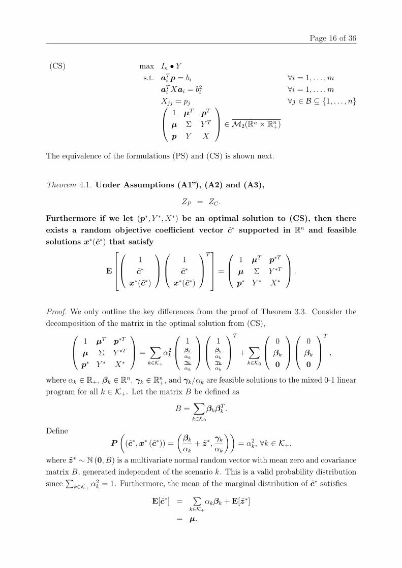
The equivalence of the formulations (PS) and (CS) is shown next.

Theorem 4.1. Under Assumptions (A1”), (A2) and (A3),

ZP = ZC .

Furthermore if we let (p∗, Y ∗, X∗) be an optimal solution to (CS), then thereexists a random objective coefficient vector c∗ supported in Rn and feasiblesolutions x∗(c∗) that satisfy

E

1

c∗

x∗(c∗)

1

c∗

x∗(c∗)

T =

1 µT p∗T

µ Σ Y ∗T

p∗ Y ∗ X∗

.

Proof. We only outline the key differences from the proof of Theorem 3.3. Consider thedecomposition of the matrix in the optimal solution from (CS),

1 µT p∗T

µ Σ Y ∗T

p∗ Y ∗ X∗

=

∑

k∈K+

α2k

1βk

αkγk

αk

1βk

αkγk

αk

T

+∑

k∈K0

0

βk

0

0

βk

0

T

,

where αk ∈ R+, βk ∈ Rn, γk ∈ Rn+, and γk/αk are feasible solutions to the mixed 0-1 linear

program for all k ∈ K+. Let the matrix B be defined as

B =∑

k∈K0

βkβTk .

DefineP

((c∗, x∗ (c∗)) =

(βk

αk

+ z∗,γk

αk

))= α2

k, ∀k ∈ K+,

where z∗ ∼ N (0, B) is a multivariate normal random vector with mean zero and covariancematrix B, generated independent of the scenario k. This is a valid probability distributionsince

∑k∈K+

α2k = 1. Furthermore, the mean of the marginal distribution of c∗ satisfies

E[c∗] =∑

k∈K+

αkβk + E[z∗]

= µ.

Page 17 of 36

Similarly, the second moment matrix satisfies

E[c∗c∗T ] =∑

k∈K+

βkβTk + E[z∗z∗T ]

=∑

k∈K+

βkβTk + B

= Σ.

Thus c∗ ∼ (µ, Σ). Finally,

supc∼(µ,Σ)+

E [Z(c)] ≥ E[Z(c∗)]

≥ E[c∗T x∗(c∗)

]

=∑

k∈K+

βTk γk +

∑k∈K+

αkE[z∗T ]γk

= In • Y ∗.

Since the right hand side is the optimal objective value of (CS), the two formulations areequivalent.

¤

Thus, by relaxing the assumption on the support of the objective coefficients, it is possibleto guarantee that the bound is exactly achievable. In computational experiments, a simplerelaxation for matrix inequality constraint in (CS) is to use

1 µT pT

µ Σ Y T

p Y X

∈M2(Rn × Rn

+) =⇒

1 µT pT

µ Σ Y T

p Y X

º 0,

(1 pT

p X

)≥ 0.

4.2. Uncertainty in Moment Information.A natural assumption to relax is the exact knowledge of moments and incorporate uncer-

tainty in the moment estimates. This is particularly useful when confidence intervals canbe built around the sample moment estimates that are often computed from the empiricaldistribution [15]. In Corollary 3.4, the assumption on the exact knowledge of the secondmoment matrix is relaxed. More generally, suppose that the exact values of the meanand the second moments are unknown, i.e. (µ, Σ) lies in a set U. In this case, the prob-lem is to choose the mean and second moment matrix and the corresponding multivariatedistribution that provides the tight bound,

(PU) sup(µ,Σ)∈U,c∼(µ,Σ)+

E [Z(c)] .

It is easy to modify CPCMM to capture the additional uncertainty,

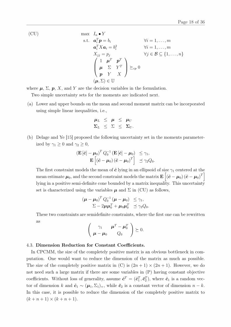
Page 18 of 36

(CU) max In • Y

s.t. aTi p = bi ∀i = 1, . . . , m

aTi Xai = b2

i ∀i = 1, . . . , m

Xjj = pj ∀j ∈ B ⊆ 1, . . . , n

1 µT pT

µ Σ Y T

p Y X

ºcp 0

(µ, Σ) ∈ Uwhere µ, Σ, p, X, and Y are the decision variables in the formulation.

Two simple uncertainty sets for the moments are indicated next.

(a) Lower and upper bounds on the mean and second moment matrix can be incorporatedusing simple linear inequalities, i.e.,

µL ≤ µ ≤ µU

ΣL ≤ Σ ≤ ΣU .

(b) Delage and Ye [15] proposed the following uncertainty set in the moments parameter-ized by γ1 ≥ 0 and γ2 ≥ 0,

(E [c]− µ0)T Q−1

0 (E [c]− µ0) ≤ γ1,

E[(c− µ0) (c− µ0)

T]¹ γ2Q0.

The first constraint models the mean of c lying in an ellipsoid of size γ1 centered at themean estimate µ0, and the second constraint models the matrix E

[(c− µ0) (c− µ0)

T]

lying in a positive semi-definite cone bounded by a matrix inequality. This uncertaintyset is characterized using the variables µ and Σ in (CU) as follows,

(µ− µ0)T Q−1

0 (µ− µ0) ≤ γ1,

Σ− 2µµT0 + µ0µ

T0 ¹ γ2Q0.

These two constraints are semidefinite constraints, where the first one can be rewrittenas (

γ1 µT − µT0

µ− µ0 Q0

)º 0.

4.3. Dimension Reduction for Constant Coefficients.In CPCMM, the size of the completely positive matrix is an obvious bottleneck in com-

putation. One would want to reduce the dimension of the matrix as much as possible.The size of the completely positive matrix in (C) is (2n + 1) × (2n + 1). However, we donot need such a large matrix if there are some variables in (P) having constant objectivecoefficients. Without loss of generality, assume cT = (cT

1 , cT2 ), where c1 is a random vec-

tor of dimension k and c1 ∼ (µ1, Σ1)+, while c2 is a constant vector of dimension n − k.In this case, it is possible to reduce the dimension of the completely positive matrix to(k + n + 1)× (k + n + 1).

Page 19 of 36

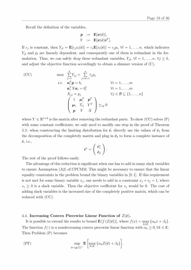
Recall the definition of the variables,

p := E[x(c)],

Y := E[x(c)cT ].

If cj is constant, then Yjl = E[cjxl(c)] = cjE[xl(c)] = cjpl, ∀l = 1, . . . , n, which indicatesYjl and pl are linearly dependent, and consequently one of them is redundant in the for-mulation. Thus, we can safely drop these redundant variables, Yjl, ∀l = 1, . . . , n, ∀j ≥ k,and adjust the objective function accordingly to obtain a slimmer version of (C),

(CC) maxk∑

j=1

Yjj +n∑

j=k+1

cjpj

s.t. aTi p = bi ∀i = 1, . . . , m

aTi Xai = b2

i ∀i = 1, . . . , m

Xjj = pj ∀j ∈ B ⊆ 1, . . . , n

1 µT1

pT

µ1 Σ1 Y T

p Y X

ºcp 0

where Y ∈ Rn×k is the matrix after removing the redundant parts. To show (CC) solves (P)with some constant coefficients, we only need to modify one step in the proof of Theorem3.3: when constructing the limiting distribution for c, directly use the values of c1 fromthe decomposition of the completely matrix and plug in c2 to form a complete instance ofc, i.e.,

c∗ =

(c∗1c2

).

The rest of the proof follows easily.The advantage of this reduction is significant when one has to add in many slack variables

to ensure Assumption (A2) of CPCMM. This might be necessary to ensure that the linearequality constraints in the problem bound the binary variables in [0, 1]. If this requirementis not met for some binary variable xj, one needs to add in a constraint xj + sj = 1, wheresj ≥ 0 is a slack variable. Then the objective coefficient for sj would be 0. The cost ofadding slack variables is the increased size of the completely positive matrix, which can bereduced with (CC).

4.4. Increasing Convex Piecewise Linear Function of Z(c).It is possible to extend the results to bound E [f (Z(c))], where f(x) = max

k∈Kαkx + βk.

The function f(·) is a nondecreasing convex piecewise linear function with αk ≥ 0,∀k ∈ K.Then Problem (P) becomes

(PF) supc∼(µ,Σ)+

E

[maxk∈K

αkZ(c) + βk].

Page 20 of 36

To obtain the corresponding CPCMM for (PF), we first partition the set of c ∈ Rn+ into

K sets with

Sk :=

c

∣∣ c ≥ 0, and αkZ(c) + βk ≥ maxk′∈K

αk′Z(c) + βk′

.

Define |K| sets of variables as follows,q(k) := P (c ∈ Sk) ,

µ(k) := E [c|c ∈ Sk] P (c ∈ Sk) ,

Σ(k) := E[ccT |c ∈ Sk

]P (c ∈ Sk) ,

p(k) := E[x(c)|c ∈ Sk]P (c ∈ Sk),

Y (k) := E[x(c)cT |c ∈ Sk]P (c ∈ Sk),

X(k) := E[x(c)x(c)|c ∈ Sk]P (c ∈ Sk).

Using a similar argument as in constructing (C), we formulate the completely positiveprogram,(CF) max

∑k∈K

(αkIn • Y (k) + βkq

(k))

s.t. aTi p(k) = biq

(k) ∀i = 1, . . . , m, ∀k ∈ KaT

i X(k)ai = b2i q

(k) ∀i = 1, . . . , m, ∀k ∈ KX

(k)jj = p

(k)j ∀j ∈ B, ∀k ∈ K

q(k) µ(k)T p(k)T

µ(k) Σ(k) Y (k)T

p(k) Y (k) X(k)

ºcp 0 ∀k ∈ K

∑k∈K

(q(k) µ(k)T

µ(k) Σ(k)

)=

(1 µT

µ Σ

)

Proving (PF) is solvable as (CF) is very similar to what we have done for Theorem 3.3,and only requires minor modifications. The key steps of the proof can be summarized asfollows.

(1) (CF) gives an upper bound to (PF).(2) Construct the extremal distribution from the optimal solution to (CF) based on the

partitions of c. With probability q(k)∗ (the value of q(k) in the optimal solution to(CF)), construct c using the completely positive decomposition of the kth matrix asin the proof of Theorem 3.3. The final limiting distribution for c would be a mixturedistribution of |K| types and satisfy the moment conditions. The decompositionalso provides the |K| sets of feasible solutions.

(3) Under the limiting distribution constructed in Step 2, the feasible solutions identi-fied achieve the upper bound in the limiting case. The nondecreasing condition forfunction f(·) is required in this step.

5. Applications

In this section, we present two applications of our model and discuss some implemen-tation issues. These applications demonstrate the usefulness and flexibility of CPCMM

Page 21 of 36

in dealing with random optimization problems. The first example deals with stochasticsensitivity analysis for the highest order statistic problem. The second example is a projectmanagement problem where the CPCMM results are compared to MMM in particular.

We also compare our results with a Monte Carlo simulation based approach. In the ap-plications we consider, the deterministic problems are linear programs with the simulationapproach needing solutions to multiple linear programs. When the deterministic problemis NP-hard, implementing the simulation method would require the solution to a numberof NP-hard problems. On the other hand, the CPP model requires the solution to oneNP-hard problem.

5.1. Stochastic Sensitivity Analysis of Highest Order Statistic.The problem of finding the maximum value from a set c = (c1, c2, . . . , cn) of n numbers

can be formulated as an optimization problem as follows,

(OS) max cT x

s.t.n∑

j=1

xj = 1

x ≥ 0

Suppose c1 > c2 > · · · > cn. Then the optimal solution to (OS) is x∗1 = 1, x∗j = 0, ∀j =

2, . . . , n. For the sensitivity analysis problem, consider a perturbation in the objectivecoefficients. Let cj = cj + εδj, ∀j = 1, . . . , n, where each δj is a random variable withmean 0 and standard deviation 1, and ε ∈ R+ is a factor that adjusts the degree of theperturbation. Then the resulting jth objective coefficient cj has mean cj and standarddeviation ε. We vary ε to see how the optimal solution changes with different degrees ofvariation in the objective coefficients.

We consider two cases: (1) Independent δj; (2) Correlated δj with E[δδT ] = Σδ. Therandom vector c ∼ (c, Σ)+, and Σ = ccT + ε2In for the independent case, while Σ =

ccT + ε2Σδ for the correlated case. The problem is to identify the probability that theoriginal optimal solution still remains optimal i.e., P (c1 ≥ cj, ∀j = 1, . . . , n) as the valueof ε increases. Moreover, P (c1 ≥ cj, ∀j = 1, . . . , n) is just the persistency of x1. We useMMM, CMM, VBC and CPCMM to estimate the probability, and then compare theirestimates against the simulation results.

Computational Results.The mean for c used in both cases, is randomly generated as

c = (19.7196, 19.0026, 17.8260, 16.4281, 15.2419, 12.1369, 9.1293, 8.8941, 4.6228, 0.3701)T ,

Page 22 of 36

and for case (2), the correlation matrix of δ, which is equal to Σδ, is

Σδ =

1 −0.5 0 0 0 0 0 0 0 0

−0.5 1 0 0 0 0 0 0 0 0

0 0 1 0.5 0.4 0 0 0 0 0

0 0 0.5 1 0.8 0 0 0 0 0

0 0 0.4 0.8 1 0 0 0 0 0

0 0 0 0 0 1 0 0 0 0

0 0 0 0 0 0 1 0 0 0

0 0 0 0 0 0 0 1 0 0

0 0 0 0 0 0 0 0 1 0

0 0 0 0 0 0 0 0 0 1

.

While we have carried out the tests on many different values of c and Σδ, the results aresimilar to what is shown here with this example.

We let ε increase from 0 to 20 at an increment of 0.1, and solve all the moment modelsfor each ε to obtain the persistency. In simulation, for each ε, we generate a 1000-sizedsample for δ satisfying the moment conditions.5 Then we solve these samples (i.e., 1000deterministic problems) to estimate P (c1 ≥ cj, ∀j = 1, . . . , n).

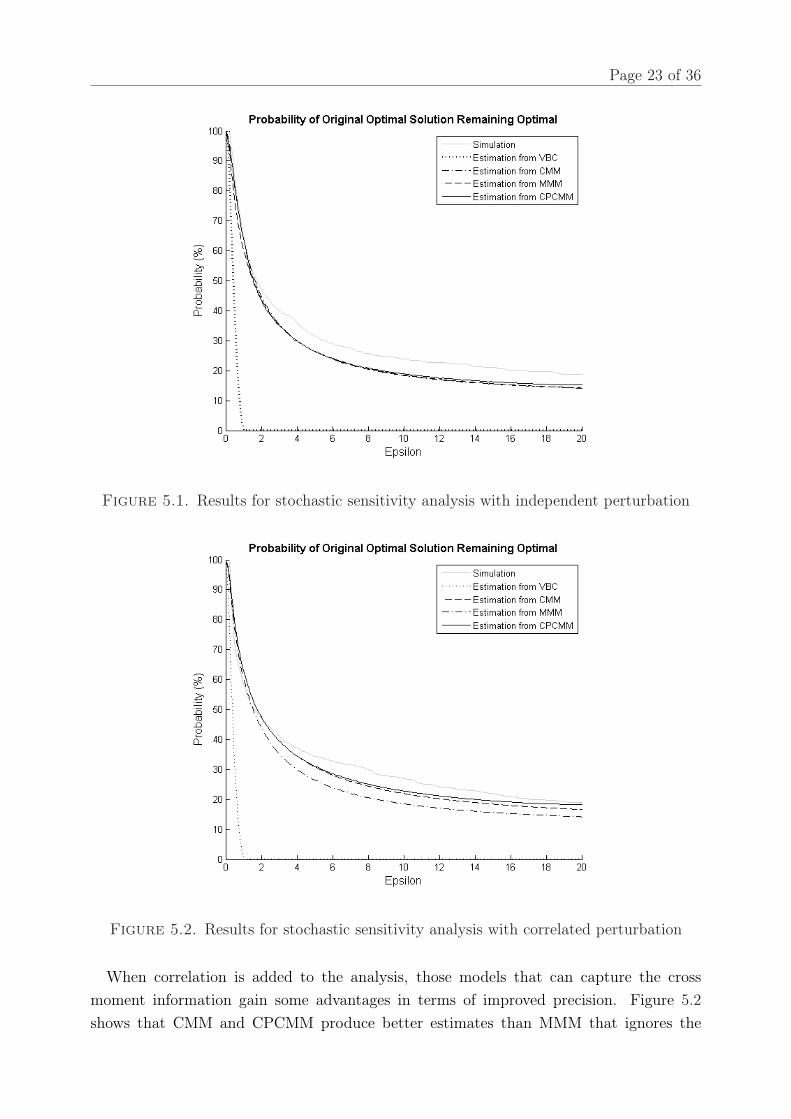
Figure 5.1 and 5.2 show the results for case (1) and (2) respectively.From Figure 5.1, we observe that the probability estimates from CPCMM and the SDP

models, except VBC, are almost the same. When ε is small, like ε < 1, the estimated valuesare almost the same as the true probabilities obtained from the simulation, and even whenε is large, the difference is not significant and the estimated curves look to have the sametrend as the simulation curve, i.e. the rate of decrease in probability is well captured bythe estimates.

Another observation is that the VBC approach gives estimates that are far away fromthe true values. The probability curve given by VBC model drops much faster and getsclose to zero quickly. There are two possible reasons. Firstly, the VBC model finds alower bound on the probability P (c1 > cj, ∀j = 2, . . . , n) which can be supported byan extreme distribution [41]. Secondly, it bounds P (c1 > cj, ∀j = 2, . . . , n) rather thanP (c1 ≥ cj, ∀j = 2, . . . , n), which would be a larger number. The results suggest that theChebyshev type bounds computed using the VBC approach might be too conservative inpractice.

5To be precise, we first generate a sample for each entry of δ independently with univariate uniform distri-bution of zero-mean and unit standard deviation. Then we apply the variance and correlation requirementsto the sample using Cholesky Decomposition method, i.e. multiplying the sample with the lower triangularmatrix obtained from the Cholesky Decomposition of the second moment matrix, Σδ. Hence, the resultingdistribution for δ will be linear combination of uniform distributions and is close to a normal distribution.The reason for using the uniform distribution is to rule out the instances where c is nonpositive, sinceAssumption (A1) for the CPCMM requires the cost coefficients to be nonnegative. Moreover, we also testthe problem with a truncated multivariate normal distribution, which gives a curve very close to the onegiven by the uniform distribution. Thus we omit it from this paper.

Page 23 of 36

Figure 5.1. Results for stochastic sensitivity analysis with independent perturbation

Figure 5.2. Results for stochastic sensitivity analysis with correlated perturbation

When correlation is added to the analysis, those models that can capture the crossmoment information gain some advantages in terms of improved precision. Figure 5.2shows that CMM and CPCMM produce better estimates than MMM that ignores the

Page 24 of 36

correlation. However, when ε is small, for example ε < 1, the three models give almost thesame estimates that are also close to the true value. Again the VBC approach provides avery conservative estimate on the probability.

From this application, we show that for simple problems with the basic approximationfor the completely positivity condition, CPCMM can perform at least as well as the otherexisting SDP models.

5.2. Project Network Problem.In this section, we apply our model on a project management problem to estimate the

expected completion time of the project and the persistency for each activity. Then we com-pare the results with MMM that ignores the cross moment information. The exponential-sized formulation of CMM is based on the number of extreme points, and thus becomesimpractical for medium to large projects.

The project management problem can be formulated as a longest path problem on adirected acyclic graph. The arcs denote activities and nodes denote completion of a set ofactivities. Arc lengths denote the time to complete the activities. Thus, the longest pathfrom the starting node s to ending node t gives the time needed to complete the project.Let cij be the length (time) of arc (activity) (i, j). The problem can be solved as a linearprogram due to the network flow structure,

max∑

(i,j)∈ARCScijxij

s.t.∑

i:(i,j)∈ARCSxij −

∑j:(i,j)∈ARCS

xji =

1, if i = s

0, if i ∈ NODES, and i 6= s, t

−1, if i = t

xij ≥ 0, ∀(i, j) ∈ ARCSFor the stochastic project management problem, the activity times are random. In such

cases, due to the resource allocation and management issues, the project manager wouldlike to focus on the activities (arcs) that are critical (lie on the longest path) with highprobabilities. Next, we demonstrate how to use CPCMM to help managers identify theseactivities.

Computational results.Consider the project network with the graphical representation shown in Figure 5.3. The

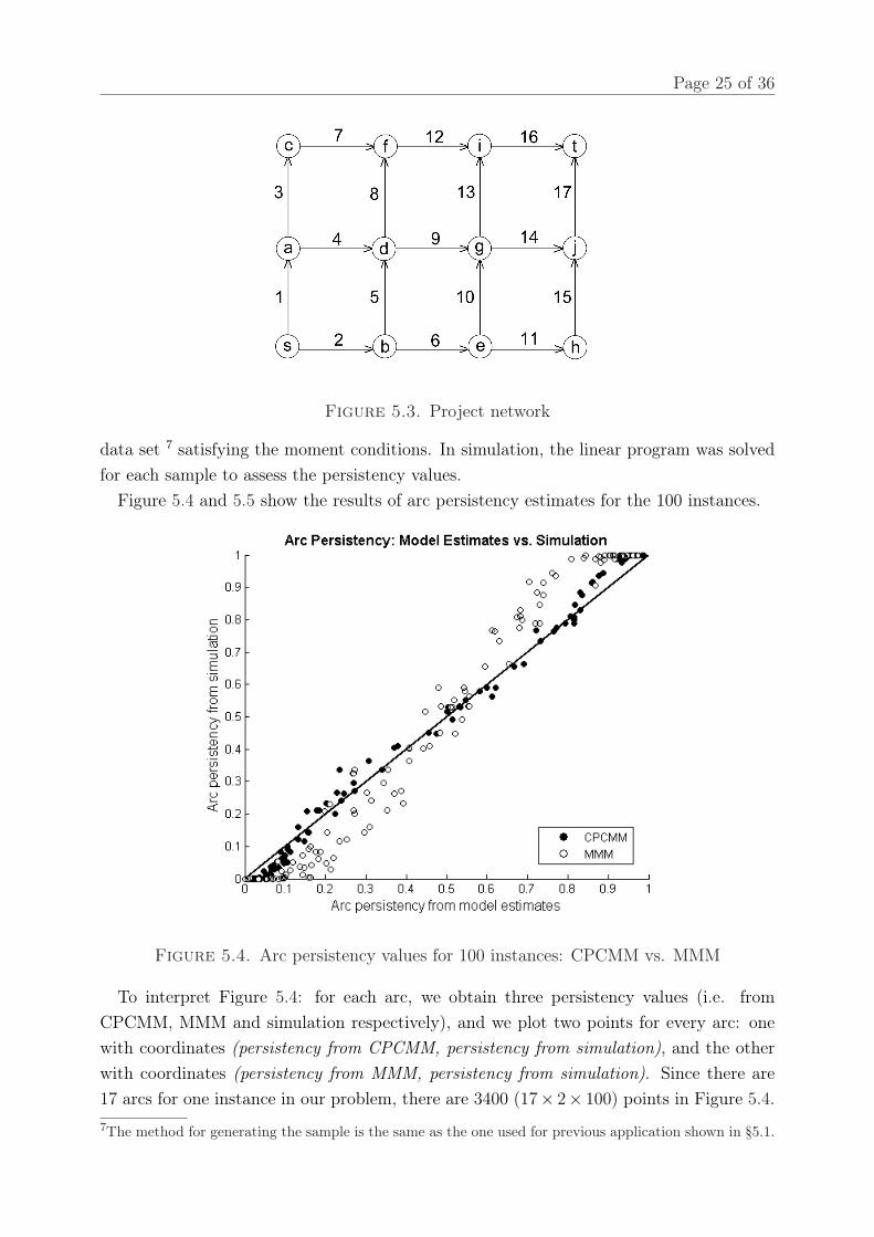
directed arcs are either upwards or to the right. This network consists of 17 arcs and 10paths.

We generate 100 data sets with each data set having a set of randomly generatedmeans (∼Uniform(0,5)), standard deviations (∼Uniform(0,2)) and correlations for the arclengths.6 CPCMM and MMM are used to estimate the persistency of each activity andexpected completion time. We resort to extensive simulations to assess the accuracy ofthe results numerically. A sample of 1000 instances of arc lengths were generated for each

6We used MATLAB function “gallery(’randcor’,n)” to generate random correlation matrices.

Page 25 of 36

Figure 5.3. Project network

data set 7 satisfying the moment conditions. In simulation, the linear program was solvedfor each sample to assess the persistency values.

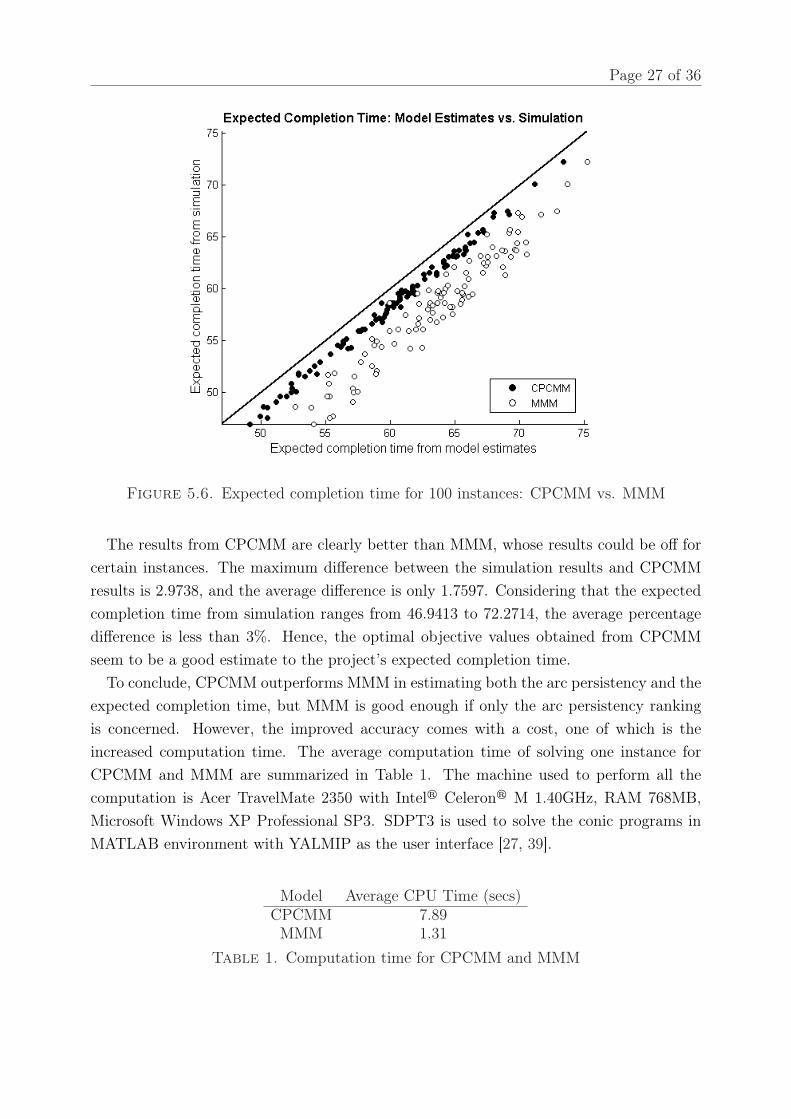
Figure 5.4 and 5.5 show the results of arc persistency estimates for the 100 instances.

Figure 5.4. Arc persistency values for 100 instances: CPCMM vs. MMM

To interpret Figure 5.4: for each arc, we obtain three persistency values (i.e. fromCPCMM, MMM and simulation respectively), and we plot two points for every arc: onewith coordinates (persistency from CPCMM, persistency from simulation), and the otherwith coordinates (persistency from MMM, persistency from simulation). Since there are17 arcs for one instance in our problem, there are 3400 (17× 2× 100) points in Figure 5.4.7The method for generating the sample is the same as the one used for previous application shown in §5.1.

Page 26 of 36

Over 94% of the persistency values are less than 0.1 which means that around 3200 pointsare clustered in the bottom left corner of Figure 5.4. The line represents the function“y = x”. Roughly it can be interpreted as the closeness of the results from the SDP modelsto simulation. If the models are perfect and the simulation is carried out with the particularextremal distribution, all the points should roughly lie on the line, while the error in theestimates is presented as a deviation from the line.

From the figure, we observe that CPCMM outperforms MMM in estimating the persis-tency values. Furthermore, we observe an “S” shaped pattern for the points plotted forboth models, which means the models tend to overestimate the small persistency valuesand underestimate the large persistency values.

Figure 5.5. Arc persistency ranking for 100 instances: CPCMM vs. MMM

For Figure 5.5, we first obtain the rankings for the persistency values from the two modelsand simulation, and then record the number of times that the rank from the models coincidewith the rank from simulation. For example, Figure 5.5 tells us that out of 100 instances,there are 99 instances for which CPCMM identifies the arc with largest persistency (rank1), while MMM identifies that in 94 instances.

Although CPCMM performs better than MMM in giving the persistency ranking, thedifference is surprisingly small as seen in the figure. This seems to suggest that MMMis good in determining the ranking of the persistency for the activities, and probablycapturing the cross moment information has very little additional value on estimating therelative criticality of the activities.

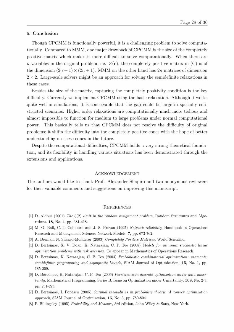
Figure 5.6 on the facing page shows the results of expected completion time for these100 instances. The way to construct the figure is similar to the one for Figure 5.4.

Page 27 of 36

Figure 5.6. Expected completion time for 100 instances: CPCMM vs. MMM

The results from CPCMM are clearly better than MMM, whose results could be off forcertain instances. The maximum difference between the simulation results and CPCMMresults is 2.9738, and the average difference is only 1.7597. Considering that the expectedcompletion time from simulation ranges from 46.9413 to 72.2714, the average percentagedifference is less than 3%. Hence, the optimal objective values obtained from CPCMMseem to be a good estimate to the project’s expected completion time.

To conclude, CPCMM outperforms MMM in estimating both the arc persistency and theexpected completion time, but MMM is good enough if only the arc persistency rankingis concerned. However, the improved accuracy comes with a cost, one of which is theincreased computation time. The average computation time of solving one instance forCPCMM and MMM are summarized in Table 1. The machine used to perform all thecomputation is Acer TravelMate 2350 with Intelr Celeronr M 1.40GHz, RAM 768MB,Microsoft Windows XP Professional SP3. SDPT3 is used to solve the conic programs inMATLAB environment with YALMIP as the user interface [27, 39].

Model Average CPU Time (secs)CPCMM 7.89MMM 1.31

Table 1. Computation time for CPCMM and MMM

Page 28 of 36

6. Conclusion

Though CPCMM is functionally powerful, it is a challenging problem to solve computa-tionally. Compared to MMM, one major drawback of CPCMM is the size of the completelypositive matrix which makes it more difficult to solve computationally. When there aren variables in the original problem, i.e. Z(c), the completely positive matrix in (C) is ofthe dimension (2n + 1)× (2n + 1). MMM on the other hand has 2n matrices of dimension2× 2. Large-scale solvers might be an approach for solving the semidefinite relaxations inthese cases.

Besides the size of the matrix, capturing the completely positivity condition is the keydifficulty. Currently we implement CPCMM using the basic relaxation. Although it worksquite well in simulations, it is conceivable that the gap could be large in specially con-structed scenarios. Higher order relaxations are computationally much more tedious andalmost impossible to function for medium to large problems under normal computationalpower. This basically tells us that CPCMM does not resolve the difficulty of originalproblems; it shifts the difficulty into the completely positive cones with the hope of betterunderstanding on these cones in the future.

Despite the computational difficulties, CPCMM holds a very strong theoretical founda-tion, and its flexibility in handling various situations has been demonstrated through theextensions and applications.

Acknowledgement

The authors would like to thank Prof. Alexander Shapiro and two anonymous reviewersfor their valuable comments and suggestions on improving this manuscript.

References

[1] D. Aldous (2001) The ζ(2) limit in the random assignment problem, Random Structures and Algo-rithms. 18, No. 4, pp. 381-418.

[2] M. O. Ball, C. J. Colbourn and J. S. Provan (1995) Network reliability, Handbook in OperationsResearch and Management Science: Network Models, 7, pp. 673-762.

[3] A. Berman, N. Shaked-Monderer (2003) Completely Positive Matrices, World Scientific.[4] D. Bertsimas, X. V. Doan, K. Natarajan, C. P. Teo (2008) Models for minimax stochastic linear

optimization problems with risk aversion, To appear in Mathematics of Operations Research.[5] D. Bertsimas, K. Natarajan, C. P. Teo (2004) Probabilistic combinatorial optimization: moments,

semidefinite programming and asymptotic bounds, SIAM Journal of Optimization, 15, No. 1, pp.185-209.

[6] D. Bertsimas, K. Natarajan, C. P. Teo (2006) Persistence in discrete optimization under data uncer-tainty, Mathematical Programming, Series B, Issue on Optimization under Uncertainty, 108, No. 2-3,pp. 251-274.

[7] D. Bertsimas, I. Popescu (2005) Optimal inequalities in probability theory: A convex optimizationapproach, SIAM Journal of Optimization, 15, No. 3, pp. 780-804.

[8] P. Billingsley (1995) Probability and Measure, 3rd edition, John Wiley & Sons, New York.

Page 29 of 36

[9] V. Borkar (1995) Probability Theory: An Advanced Course, Editorial Board: S. Axler, F. W. Gehring,P. R. Halmos, Springer, New York.

[10] B. Bollobas, D. Gamarnik, O. Riordan and B. Sudakov (2004) On the value of a random minimumlength Steiner Tree, Combinatorica, 24, No. 2, pp. 187-207.

[11] I. M. Bomze, M. Dür, E. D. Klerk, C. Roos, A. J. Quist, T. Terlaky (2000) On copositive programmingand standard quadratic optimization problems, Journal of Global Optimization, 18, No. 4, pp. 301-320.

[12] S. Burer (2009) On the copositive representation of binary and continuous nonconvex quadratic pro-grams, Mathematical Programming, 120, No. 2, pp. 479-495.

[13] G. Calafiore, L. E. Ghaoui (2006) On distributionally robust chance-constrained linear programs, Op-timization Theory and Applications, 130, No. 1, pp. 1-22.

[14] R. Davis, A. Prieditis (1993) The expected length of a shortest path, Information Processing Letters,46, No. 3, pp. 135-141.

[15] E. Delage, Y. Ye (2008) Distributionally robust optimization under moment uncertainty with applica-tion to data-driven problems, To appear in Operations Research.

[16] M. Dür, G. Still (2007) Interior points of the completely positive cone, Electronic Journal of LinearAlgebra, 17, pp. 48-53.

[17] A. M. Frieze (1985) On the value of a random minimum spanning tree problem, Discrete AppliedMathematics, 10, No. 1, pp. 47-56.

[18] J. N. Hagstrom (1988) Computational complexity of PERT problems, Networks, 18, No. 2, pp. 139-147.[19] K. Isii (1959) On a method for generalizations of Tchebycheff’s inequality, Annals of the Institute of

Statistical Mathematics, 10, pp. 65-88.[20] S. Karlin, S. Studden (1966) Tchebycheff Systems: with Applications in Analysis and Statistics, John

Wiley & Sons.[21] J. H. B. Kemperman, M. Skibinsky (1993) Covariance spaces for measures on polyhedral sets, Sto-

chastic Inequalities, Institute of Mathematical Statistics Lecture Notes - Monograph Series, 22, pp.182-195.

[22] E. de Klerk, D. V. Pasechnik (2002) Approximation of the stability number of a graph via copositiveprogramming, SIAM Journal on Optimization, 12, No. 4, pp. 875-892.

[23] V. G. Kulkarni (1986) Shortest paths in networks with exponentially distributed arc capacities, Net-works, 18, pp. 111-124.

[24] J. Lasserre (2002) Bounds on measures satisfying moment conditions, The Annals of Applied Proba-bility, 12, No. 3, pp. 1114-1137.

[25] J. Lasserre (2010) A "Joint+Marginal" approach to parametric polynomial optimization, To appearin SIAM Journal of Optimization.

[26] S. Linusson, J. Wästlund (2004) A proof of Parisi’s conjecture on the random assignment problem,Probability Theory and Related Fields, 128, 419-440.

[27] J. Löfberg (2004) YALMIP: A Toolbox for Modeling and Optimization in MATLAB, In Proceedingsof the CACSD Conference, Taipei, Taiwan, available at http://control.ee.ethz.ch/ joloef/yalmip.php.

[28] R. Lyons, R. Pemantle, Y. Peres (1999) Resistance bounds for first-passage percolation and maximumflow, Journal of Combinatorial Theory Series A, 86, No. 1, pp. 158-168.

[29] M. Mézard, G. Parisi (1987) On the solution of the random link matching problems, Journal dePhysique Lettres, 48, pp. 1451-1459.

[30] V. K. Mishra, K. Natarajan, H. Tao, C-P. Teo (2008) Choice modeling with semidefinite optimizationwhen utilities are correlated, Submitted.

[31] K. G. Murty, S. N. Kabadi (1987) Some NP-complete problems in quadratic and nonlinear program-ming, Mathematical Programming, 39, No. 2, pp. 117-129.

Page 30 of 36

[32] C. Nair, B. Prabhakar, M. Sharma (2006) Proofs of the Parisi and Coppersmith-Sorkin random as-signment conjectures, Random Structures and Algorithms, 27, No. 4, pp. 413-444.

[33] K. Natarajan, M. Song, C. P. Teo (2009) Persistency model and its applications in choice modeling,Management Science, 55, No. 3, pp. 453-469.

[34] Y. Nesterov (2000) Squared functional systems and optimization problems, In: High PerformanceOptimization, Kluwer Academic Press, pp. 405-440.

[35] P. A. Parrilo (2000) Structured Semidefinite Programs and Semi-algebraic Geometry Methods in Ro-bustness and Optimization, Ph.D. thesis, California Institute of Technology, Pasadena, CA, availableonline at: http://www.cds.caltech.edu/~pablo/.

[36] I. Popescu (2007) Robust mean-covariance solutions for stochastic optimization, Operations Research,55, No. 1, pp. 98-112.

[37] J. S. Provan, M. O. Ball (1983) The complexity of counting cuts and of computing the probability thata graph is connected, SIAM Journal on Computing, 12, No. 4, pp. 777-788.

[38] M. J. Todd (2001) Semidefinite optimization, Acta Numerica, 10, pp. 515-560.[39] K. C. Toh, M. J. Todd, R. H. Tutuncu (1999) SDPT3 — a Matlab software package for semidefinite

programming, Optimization Methods and Software, 11, pp. 545-581.[40] L. G. Valiant (1979) The complexity of enumeration and reliability problems, SIAM Journal on Com-

puting, 8, pp. 410-442.[41] L. Vandenberghe, S. Boyd, K. Comanor (2007) Generalized Chebyshev bounds via semidefinite pro-

gramming, SIAM Review, 49, No. 1, pp. 52-64.[42] J. Wästlund (2009) The mean field traveling salesman and related problems[43] L. Zuluaga, J. F. Pena (2005) A conic programming approach to generalized Tchebycheff inequalities,

Mathematics of Operations Research, 30, No. 2, pp. 369-388.

Page 31 of 36

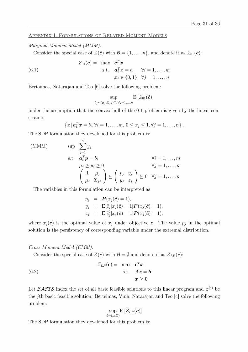
Appendix I. Formulations of Related Moment Models

Marginal Moment Model (MMM).Consider the special case of Z(c) with B = 1, . . . , n, and denote it as Z01(c):

(6.1)Z01(c) = max cT x

s.t. aTi x = bi ∀i = 1, . . . , m

xj ∈ 0, 1 ∀j = 1, . . . , n

Bertsimas, Natarajan and Teo [6] solve the following problem:

supcj∼(µj ,Σjj)

+, ∀j=1,...,n

E [Z01(c)]

under the assumption that the convex hull of the 0-1 problem is given by the linear con-straints

x|aTi x = bi,∀i = 1, . . . , m, 0 ≤ xj ≤ 1,∀j = 1, . . . , n

.

The SDP formulation they developed for this problem is:

(MMM) supn∑

j=1

yj

s.t. aTi p = bi ∀i = 1, . . . , m

µj ≥ yj ≥ 0 ∀j = 1, . . . , n(1 µj

µj Σjj

)º

(pj yj

yj zj

)º 0 ∀j = 1, . . . , n

The variables in this formulation can be interpreted as

pj = P (xj(c) = 1),

yj = E[cj|xj(c) = 1]P (xj(c) = 1),

zj = E[c2j |xj(c) = 1]P (xj(c) = 1).

where xj(c) is the optimal value of xj under objective c. The value pj in the optimalsolution is the persistency of corresponding variable under the extremal distribution.

Cross Moment Model (CMM).Consider the special case of Z(c) with B = ∅ and denote it as ZLP (c):

(6.2)ZLP (c) = max cT x

s.t. Ax = b

x ≥ 0

Let BASIS index the set of all basic feasible solutions to this linear program and x(j) bethe jth basic feasible solution. Bertsimas, Vinh, Natarajan and Teo [4] solve the followingproblem:

supc∼(µ,Σ)

E [ZLP (c)]

The SDP formulation they developed for this problem is:

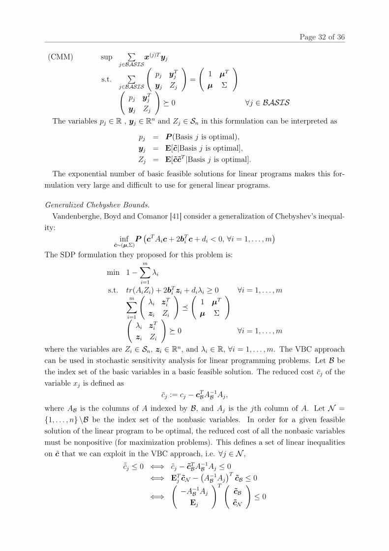
Page 32 of 36

(CMM) sup∑

j∈BASISx(j)T yj

s.t.∑

j∈BASIS

(pj yT

j

yj Zj

)=

(1 µT

µ Σ

)

(pj yT

j

yj Zj

)º 0 ∀j ∈ BASIS

The variables pj ∈ R , yj ∈ Rn and Zj ∈ Sn in this formulation can be interpreted as

pj = P (Basis j is optimal),yj = E[c|Basis j is optimal],Zj = E[ccT |Basis j is optimal].

The exponential number of basic feasible solutions for linear programs makes this for-mulation very large and difficult to use for general linear programs.

Generalized Chebyshev Bounds.Vandenberghe, Boyd and Comanor [41] consider a generalization of Chebyshev’s inequal-

ity:inf

c∼(µ,Σ)P

(cT Aic + 2bT

i c + di < 0, ∀i = 1, . . . , m)

The SDP formulation they proposed for this problem is:

min 1−m∑

i=1

λi

s.t. tr(AiZi) + 2bTi zi + diλi ≥ 0 ∀i = 1, . . . , m

m∑i=1

(λi zT

i

zi Zi

)¹

(1 µT

µ Σ

)

(λi zT

i

zi Zi

)º 0 ∀i = 1, . . . , m

where the variables are Zi ∈ Sn, zi ∈ Rn, and λi ∈ R, ∀i = 1, . . . , m. The VBC approachcan be used in stochastic sensitivity analysis for linear programming problems. Let B bethe index set of the basic variables in a basic feasible solution. The reduced cost cj of thevariable xj is defined as

cj := cj − cTBA−1

B Aj,

where AB is the columns of A indexed by B, and Aj is the jth column of A. Let N =

1, . . . , n \B be the index set of the nonbasic variables. In order for a given feasiblesolution of the linear program to be optimal, the reduced cost of all the nonbasic variablesmust be nonpositive (for maximization problems). This defines a set of linear inequalitieson c that we can exploit in the VBC approach, i.e. ∀j ∈ N ,

¯cj ≤ 0 ⇐⇒ cj − cTBA−1

B Aj ≤ 0

⇐⇒ ETj cN −

(A−1B Aj

)TcB ≤ 0

⇐⇒(−A−1

B Aj

Ej

)T (cBcN

)≤ 0

Page 33 of 36

Hence, these |N | inequalities can be viewed as a set constraining c,

CLP =

c ∈ Rn

∣∣∣∣∣∣

(−A−1

B Aj

Ej

)T

c ≤ 0, ∀j ∈ N .

Then any realization of c falling in this set (i.e. c ∈ CLP ) will make the pre-given feasiblesolution optimal. Therefore, the probability that c lies in the set is just the probabilitythat the given feasible solution is optimal. Furthermore, when A is of rank one, i.e. thereis only one basic variable in any feasible solution, that probability is just the persistency ofthat particular basic variable. One difference between CLP and C in the VBC approach isthat all the inequalities in C are strict, so when we apply the VBC model to this problem,the interpretation of the resulting probability has to be changed to the probability thatthe given feasible solution is the unique optimum. Using the VBC approach on the LPproblem, we obtain:(VBC) min 1− ∑

j∈Nλj

s.t.

(−A−1

B Aj

Ej

)T

zj ≥ 0 ∀j ∈ N

∑j∈N

(Zj zj

zTj λj

)¹

(Σ µ

µT 1

)

(Zj zj

zTj λj

)º 0 ∀j ∈ N

Thus, for any given feasible solution, we can solve the corresponding (VBC) and obtainthe optimal objective value, which is the tightest lower bound on the probability that thegiven feasible solution is the unique optimal solution to Problem (6.2).

Page 34 of 36

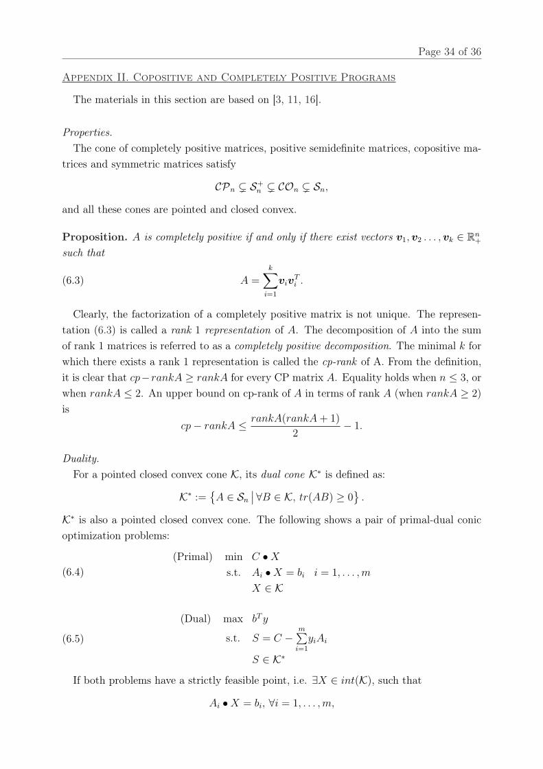
Appendix II. Copositive and Completely Positive Programs

The materials in this section are based on [3, 11, 16].

Properties.The cone of completely positive matrices, positive semidefinite matrices, copositive ma-

trices and symmetric matrices satisfy

CPn ( S+n ( COn ( Sn,

and all these cones are pointed and closed convex.

Proposition. A is completely positive if and only if there exist vectors v1, v2 . . . , vk ∈ Rn+

such that

(6.3) A =k∑

i=1

vivTi .

Clearly, the factorization of a completely positive matrix is not unique. The represen-tation (6.3) is called a rank 1 representation of A. The decomposition of A into the sumof rank 1 matrices is referred to as a completely positive decomposition. The minimal k forwhich there exists a rank 1 representation is called the cp-rank of A. From the definition,it is clear that cp−rankA ≥ rankA for every CP matrix A. Equality holds when n ≤ 3, orwhen rankA ≤ 2. An upper bound on cp-rank of A in terms of rank A (when rankA ≥ 2)is

cp− rankA ≤ rankA(rankA + 1)

2− 1.

Duality.For a pointed closed convex cone K, its dual cone K∗ is defined as:

K∗ :=A ∈ Sn

∣∣ ∀B ∈ K, tr(AB) ≥ 0

.

K∗ is also a pointed closed convex cone. The following shows a pair of primal-dual conicoptimization problems:

(6.4)(Primal) min C •X

s.t. Ai •X = bi i = 1, . . . , m

X ∈ K

(6.5)

(Dual) max bT y

s.t. S = C −m∑

i=1

yiAi

S ∈ K∗

If both problems have a strictly feasible point, i.e. ∃X ∈ int(K), such that

Ai •X = bi, ∀i = 1, . . . , m,

Page 35 of 36

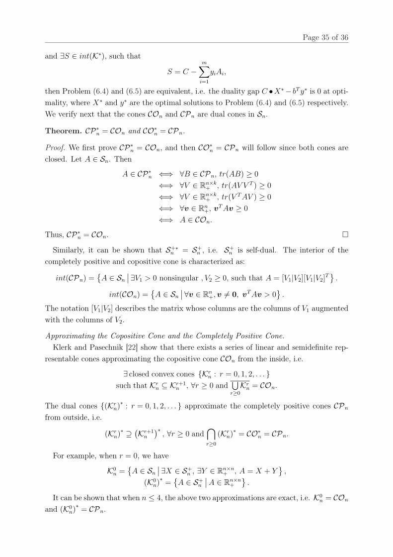
and ∃S ∈ int(K∗), such that

S = C −m∑

i=1

yiAi,

then Problem (6.4) and (6.5) are equivalent, i.e. the duality gap C •X∗− bT y∗ is 0 at opti-mality, where X∗ and y∗ are the optimal solutions to Problem (6.4) and (6.5) respectively.We verify next that the cones COn and CPn are dual cones in Sn.

Theorem. CP∗n = COn and CO∗n = CPn.

Proof. We first prove CP∗n = COn, and then CO∗n = CPn will follow since both cones are

closed. Let A ∈ Sn. Then

A ∈ CP∗n ⇐⇒ ∀B ∈ CPn, tr(AB) ≥ 0

⇐⇒ ∀V ∈ Rn×k+ , tr(AV V T ) ≥ 0

⇐⇒ ∀V ∈ Rn×k+ , tr(V T AV ) ≥ 0

⇐⇒ ∀v ∈ Rn+, vT Av ≥ 0

⇐⇒ A ∈ COn.

Thus, CP∗n = COn. ¤

Similarly, it can be shown that S+∗n = S+

n , i.e. S+n is self-dual. The interior of the

completely positive and copositive cone is characterized as:

int(CPn) =A ∈ Sn

∣∣ ∃V1 > 0 nonsingular , V2 ≥ 0, such that A = [V1|V2][V1|V2]T

.

int(COn) =A ∈ Sn

∣∣ ∀v ∈ Rn+, v 6= 0, vT Av > 0

.

The notation [V1|V2] describes the matrix whose columns are the columns of V1 augmentedwith the columns of V2.

Approximating the Copositive Cone and the Completely Positive Cone.Klerk and Pasechnik [22] show that there exists a series of linear and semidefinite rep-

resentable cones approximating the copositive cone COn from the inside, i.e.

∃ closed convex cones Krn : r = 0, 1, 2, . . .

such that Krn ⊆ Kr+1

n , ∀r ≥ 0 and⋃r≥0

Krn = COn.

The dual cones (Krn)∗ : r = 0, 1, 2, . . . approximate the completely positive cones CPn

from outside, i.e.

(Krn)∗ ⊇ (Kr+1

n

)∗, ∀r ≥ 0 and

⋂r≥0

(Krn)∗ = CO∗

n = CPn.

For example, when r = 0, we have

K0n =

A ∈ Sn

∣∣ ∃X ∈ S+n , ∃Y ∈ Rn×n

+ , A = X + Y

,

(K0n)∗

=A ∈ S+

n

∣∣ A ∈ Rn×n+

.

It can be shown that when n ≤ 4, the above two approximations are exact, i.e. K0n = COn

and (K0n)∗

= CPn.

Page 36 of 36

The higher order approximation (r ≥ 1) becomes much more complicated. For instance,when r = 1, Parrilo (2000, [35]) showed that

K1n =

A ∈ Sn

∣∣∣∣∣∣∣∣∣

∃M (i) ∈ Sn, i = 1, 2 . . . , n

such that

A−M (i) º 0, i = 1, 2 . . . , n

M(i)ii = 0, i = 1, 2 . . . , n

M(i)jj + M

(j)ij + M

(j)ji = 0, i 6= j

M(i)jk + M

(j)ik + M

(k)ij ≥ 0, i 6= j 6= k

.