Multi-dimensional Latent Group Structures with ...

Multi-dimensional Latent Group Structures with Heterogeneous

Distributions

Xuan Lenga Heng Chenb Wendun Wangc

September 9, 2021

Abstract

This paper aims to identify the multi-dimensional latent grouped heterogeneity of distributional

effects. We consider a panel quantile regression model with additive cross-section and time fixed

effects. The cross-section effects and quantile slope coefficients are both characterized by grouped

patterns of heterogeneity, but each unit can belong to different groups for cross-section effects and

slopes. We propose a composite-quantile approach to jointly estimate multi-dimensional group

memberships, slope coefficients, and fixed effects. We show that using multiple quantiles improves

clustering accuracy if memberships are quantile-invariant. We apply the methods to examine the

relationship between managerial incentives and risk-taking behavior.

Keywords: Composite quantile estimation, distributional heterogeneity, latent groups, panel

quantile regressions, two-way fixed effects

JEL Classification: C31, C33, C38, G31, J33

[email protected]. MOE Key Laboratory of Econometrics, Wang Yanan Institute for Studies in Economics, De-

partment of Statistics and Data Science at School of Economics, and Fujian Key Lab of Statistics, Xiamen University,

422 Siming S Rd, Siming District, Xiamen, Fujian, China, [email protected]. Currency Department, Bank of Canada, 234 Wellington St. W, Ottawa, ON K1A 0G9cCorresponding author. [email protected]. Econometric Institute, Erasmus University Rotterdam and Tinbergen

Institute, Burg. Oudlaan 50, 3062 PA Rotterdam, Netherlands

1

1 Introduction

The two-way fixed effects model has emerged as a common practice to analyze panel data in economics

and finance as it allows researchers to control for unobserved heterogeneity in both cross-sectional and

time-series dimensions. A salient empirical finding in panel data applications shows that the effect

of covariates often exhibits a grouped pattern of heterogeneity, that is, homogeneous effects within a

group (see, e.g., Mitton, 2002; Browning and Carro, 2007; Duchin et al., 2010, among many others),

even when unobserved heterogeneity is accounted for. Hahn and Moon (2010) provided a theoretical

foundation for group heterogeneity and Bonhomme et al. (2017) argued that group heterogeneity

can be a good discrete approximation even if individual heterogeneity is present. Existing studies

on panel group heterogeneity primarily focus on the (conditional) mean effects and cluster units

based on the mean heterogeneity. However, in many applications, it is empirically useful to unveil

the distributional effects of covariates and model the distributional heterogeneity (i.e., the difference

in distributional effects across groups). For example, the impact of managerial incentives on R&D

expenditure seems to vary across different levels of R&D expenditure, and such distributional effects

may also vary across firms with distinct firm and managerial features. Hence, it is desirable for decision

makers and investors to understand the heterogeneous distributional effects of managerial incentives on

innovation-investment decisions. Moreover, it is crucial to control for unobserved cross-sectional and

time heterogeneity in this study because investment decisions are obviously influenced by unobserved

firm risk-taking strategies and various market events over the years.

This study presents a new model and estimation method to capture grouped patterns of distri-

butional heterogeneity of covariate effects, while at the same time controlling for unobserved hetero-

geneity in both cross-sectional and time dimensions. We consider panel quantile regression models

with additive cross-section and time fixed effects and allow the quantile slope coefficients to be group

specific, such that units in the same group share common (conditional) distributional effects, while

the distributions may differ across groups in the location, shape, or both. Moreover, the cross-section

fixed effects are also characterized by a grouped pattern of heterogeneity in a similar spirit of Bon-

homme and Manresa (2015a) and Gu and Volgushev (2019), but the associated group membership

structure can differ from that of slope coefficients. In other words, each unit can belong to different

groups for cross-section fixed effects and slope coefficients. The two group membership structures are

both unknown, and we aim at identifying the two latent group structures (i.e., which units belongs to

which group), leading to a multi-dimensional clustering problem. Modelling multi-dimensional group

structures permits different degrees of heterogeneity in cross-section effects and slope coefficients, such

that units in one group share a common coefficient vector but can differ in fixed effects, or vice versa.

In contrast, one-dimensional clustering requires homogeneity of both cross-section effects and slopes

within a group, and therefore cuts the data finer, rendering some groups with only a few units and

of much smaller size than the others (also referred to as sparse interactions by Cheng et al. (2019);

see also Cytrynbaum (2020) for related discussions). A small number of units in a group may lead to

inaccurate or sometimes even infeasible estimation of group-specific parameters, especially when the

2

number of group-specific parameters is close or even larger than the number of observations in this

group. Inaccurate estimation of group-specific parameters in turn deteriorates the clustering perfor-

mance. Therefore, by imposing less strict requirements of homogeneity in a group, multi-dimensional

clustering offers an effective and more flexible way of capturing cross-sectional heterogeneity than

one-dimensional clustering. While our model and estimation approach allow group memberships to be

dependent or common over quantiles, we focus on the latter case of quantile-invariant memberships,

which is relevant in many empirical applications.1 The quantile-invariant group structure allows us to

pool information across quantiles to improve the group membership estimates.

We jointly estimate the multi-dimensional group memberships, slope coefficients, and fixed effects

by minimizing a composite quantile check function, that is, a sum of the quantile check functions across

different quantile levels over which the group structures are common. The composite quantile objec-

tive function allows us to utilize the information of group structures contained at multiple quantiles

simultaneously and facilitates clustering. To solve the optimization problem, we employ an iterative

algorithm that alters between group membership estimation and panel quantile regression estimation,

similar in spirit to K-means clustering. In addition to establishing the consistency of membership

and coefficient estimators, we comprehensively quantify the speed of convergence of the misclustering

frequency (MF), a measure of clustering accuracy. We show that the speed of convergence is an expo-

nential function of the length of time periods and that it depends on the number of quantiles used for

clustering, degree of group separation, signal-to-noise ratio, and serial correlation of data. To the best

of our knowledge, this is the first study that precisely quantifies how the clustering accuracy depends

on the use of composite quantiles model and the features of data in the panel group structure litera-

ture.2 We explicitly show that pooling information of multiple quantiles improves clustering accuracy

if the group structure is invariant over these quantiles.

Our model is related with the burgeoning literature on panel structure models, for example, the

K-means type of methods (Lin and Ng, 2012; Bonhomme and Manresa, 2015a; Liu et al., 2020;

Ando and Bai, 2016; Vogt and Linton, 2016; Miao et al., 2020), Lasso-type of approaches (Su et al.,

2016; Wang et al., 2018), pairwise comparisons (Krasnokutskaya et al., 2021), binary segmentation

(Ke et al., 2016; Su and Wang, 2021), among others. More recently, Cheng et al. (2019) studied

the multi-dimensional clustering in the presence of endogenous regressors. These methods cluster

units based on the heterogeneity of conditional mean effects, while our work captures the grouped

heterogeneity in the distributional effects. Sun (2005); Rosen et al. (2000); Ng and McLachlan (2014),

1In practice, group memberships are often driven by a few “inertial” factors that hardly vary across the distributionof the dependent variable. For example, Brand and Xie (2010) found that the economic returns of education differsignificantly across individuals depending on how likely they are to attend college. Since the likelihood of attendingcollege typically does not change over wage distribution, it seems plausible that the membership structure is also invariantto quantiles. Zwick and Mahon (2017) showed that firms’ decisions to invest in equipment are affected by temporarytax incentives, and small firms respond far more actively to tax incentives than large firms do. Again, such underlyingheterogeneity (size of a firm) varies little across the distribution of investment levels. The quantile-specific membershipscan be easily incorporated in our estimation framework as will be clear in Section 2.2.

2Existing studies in the panel data classification literature only provide the consistency of the group membershipestimates or show the convergence rate of the MF as an exponential function of the time-series dimension and someunknown number, such as Bonhomme and Manresa (2015a), Okui and Wang (2021), and Zhang et al. (2019a). They donot explain how data features influence clustering accuracy.

3

among others, considered a finite mixture of latent conditional distributions to model the distributional

heterogeneity. These studies often assumed that the mixture probability depends on some observables

or that the mixture distribution is composed of several known distributions. In contrast, we allow

the group memberships and the distributions to be fully unrestricted. Another way of capturing the

grouped pattern of distributional heterogeneity is to cluster units based on the empirical cumulative

distribution function (CDF). Bonhomme et al. (2019) proposed to recover latent firm classes based on

the empirical CDF of the earning distributions in an employer-employee matching study. Compared

with empirical CDF-based clustering, regression quantiles may provide more detailed information on

the distribution and thus stronger group separation, which further facilitates clustering.

This study also builds on a large amount of existing literature on panel quantile regression models.

Following the seminal research of Koenker (2004), several influential studies have provided strict

(asymptotic) analysis on the estimation and inference of panel quantile regressions with individual

fixed effects, such as Galvao (2011), Kato et al. (2012), Galvao and Kato (2016) and Yoon and Galvao

(2020), among many others. All these studies assume that the quantile regression coefficients are

common across units. In contrast, we relax the cross-section homogeneity assumption and allow

the quantile-specific coefficients to differ across units via a latent grouped pattern. Since our model

contains time fixed effects, we need to deal with the incidental-parameter issue in the time dimension,

in the similar spirit but symmetric to the existing studies that consider individual fixed effects. We

show the consistency of the quantile slope estimates for each group, and use a similar idea as Galvao

et al. (2020) to show the asymptotic normality of these estimates under a mild growth condition of

the sample sizes. Chetverikov et al. (2016) considered a panel quantile regression with unit-specific

slope coefficients, and model such heterogeneous slopes as a linear combination of a set of observed

unit-level covariates. While allowing for a richer degree of heterogeneity than a group pattern, their

model assumes a specific form of heterogeneity. If we regard those unit-level covariates as an indicator

of the group memberships of units, this model can be viewed as a special case of panel quantile group

structure models but with a known group membership structure. In contrast, we model the cross-

sectional heterogeneity via latent and unrestricted group patterns, and we aim at identifying the latent

group structures.

Two closely related works include Gu and Volgushev (2019) and Zhang et al. (2019a). Gu and

Volgushev (2019) considered panel quantile regressions with grouped fixed effects and homogeneous

slope coefficients, and cluster units based on a single quantile. We generalize their model by allowing

time fixed effects and group heterogeneity in slopes. Moreover, when the group structure is invariant

to quantiles, our composite-quantile estimation ensures that the estimated memberships are common

over quantiles and also more accurate than those estimated using a single quantile. Zhang et al. (2019a)

considered a panel quantile model allowing for group-specific slopes and individual-specific fixed effects.

We differ from this work by considering both cross-section and time fixed effects and allowing for multi-

dimensional group heterogeneity. Moreover, our asymptotic analysis complements Zhang et al. (2019a)

by explicitly showing how the use of multiple quantiles influence clustering accuracy. While Zhang

et al. (2019a) documented the advantages of the composite-quantile estimation via simulation, strict

4

theoretical justifications are missing.

We illustrate the economic importance of accounting for grouped heterogeneity in the distribu-

tional effects by revisiting the relationship between managerial incentives and risk-taking behavior

measured by R&D expenditure. We find a significant degree of heterogeneity in the relationship be-

tween managerial incentives and risk-taking behavior across groups and across different locations of

the conditional distribution of R&D expenditure. The grouped pattern is related with, yet sufficiently

differs from industry grouping often imposed by applied finance researchers. The distributional het-

erogeneity and multi-dimensional latent groups in cross-section effects and slopes can be captured by

our panel structure quantile regression models, but not by conventional linear panel regressions with

two-way fixed effects.

The rest of the paper is organized as follows. Section 2 sets up the model and presents the

estimation method given the number of groups. Section 3 provides the asymptotic properties of the

proposed estimators. Section 4 discusses how to determine the number of groups. Section 5 presents

the simulation study, and Section 6 discusses an empirical application. Section 7 concludes. The

technical details are organized in the Supplementary Appendix.

2 Model setup and estimation

In this section, we first describe the setup of our model, and then explain the estimation approach.

2.1 Model setup

Suppose we observe yit, xiti=1,...,N,t=1,...,T , where yit is the scalar dependent variable of individual

i observed at time t, and xit is a p × 1 vector of exogenous regressors. We are interested in the

effect of xit on the conditional quantile of yit. Due to cross-sectional heterogeneity, the conditional

quantile effect may vary across units (Galvao et al., 2017). We assume that the heterogeneous quantile

effects can be characterized by a grouped pattern, such that units of the same group share a common

conditional quantile effect. In addition, we allow for both cross-section and time fixed effects in

the model, where the cross-section effects also exhibit a group pattern in a similar spirit of Gu and

Volgushev (2019), while their group membership structure can differ from that of slope coefficients in

an arbitrary manner. We write the model as

Qτ (yit|xit) = αhi(τ) + λt(τ) + x′itβgi(τ), i = 1, . . . , N, t = 1, . . . , T, (2.1)

where Qτ (yit|xit) is the conditional τ -quantile of yit given xit with τ ∈ (0, 1), αhi(τ) and λt(τ) denote

the cross-section and time fixed effects, and βgi(τ) is the group-specific quantile regression coefficient.

The subscripts hi ∈ 1, . . . ,H and gi ∈ 1, . . . , G denote the group memberships of unit i for cross-

section fixed effects α(τ) and slope coefficients β(τ), respectively, where H < ∞ and G < ∞ are

the number of groups. Importantly, we allow the group structures of cross-section effects and slope

coefficients both to be latent, which may depend on (possibly high-dimensional) observed and unob-

5

served covariates in an unrestricted manner. Such flexibility allows us to capture rich heterogeneity

in a wide range of applications, even though G and H are assumed fixed and finite. Here we focus

on the case where the group membership structure hi, giNi=1 is time-invariant and independent of

a range of quantiles, which is not an uncommon situation in practice. We refer to this model as

multi-dimensional group structure quantile regressions (MuGS-QR).

Model (2.1) includes several important models as special cases. When τ = 0.5, hi = gi for all i,

and there are no time fixed effects, our model collapses to a median regression with a single-level group

structure of heterogeneity, which is closely related to the panel structure model with the group-specific

conditional mean effects (Lin and Ng, 2012; Su et al., 2016). When the time fixed effects are absent

and βgi(τ) is cross-sectionally homogeneous, our model reduces to the panel quantile grouped-specific

fixed effects specification by Gu and Volgushev (2019), which extends the conditional mean grouped

fixed effects (GFE) model of Bonhomme and Manresa (2015a). Since our model includes the time

effects, we do face the incidental parameter problem as Zhang et al. (2019a) and Galvao et al. (2020)

but in the time dimension, and some of our theoretical conditions are comparable to those of Galvao

et al. (2020) by swapping the role of N and T . Our model can also be viewed as a quantile version

of multi-dimensional clustering for panel mean regressions in Cheng et al. (2019), and we additionally

allow for time effects but focus on exogenous regressors.

In model (2.1), we can identify the two latent group structures by using the time series of all

units.3 We discuss the group identifiability from the following two aspects. First, we can identify

the latent group memberships for each individual if s/he has sufficient time observations lying in the

non-overlapping region of the two groups. This is satisfied if one can observe each unit for infinitely

many periods. Second, we allow the distribution of a group to be of any shape, including the multi-

modal distribution, and can still correctly identify the group membership structures. Again, this is

achieved by observing each unit for infinitely many periods. For example, if a group is characterized

by a bimodal distribution, it would not be identified as two unimodal groups because the distribution

of each unit in this group is bimodal.

2.2 Estimation method

There are two types of parameters in model (2.1): (i) the group membership variables gii=1,...,N and

hii=1,...,N for the g-group and h-group structure, respectively; (ii) the regression quantile param-

eters βg(τ) ∈ B, αh(τ) ∈ A, and λt(τ) ∈ D for each fixed τ . Define β(τ) := β′1(τ), . . . , β′G(τ)′,α(τ) := α1(τ), . . . , αH(τ)′, and λ(τ) := λ1(τ), . . . , λT (τ)′. In practice, we consider a finite

quantile sequence τ := (τ1, . . . , τK)′, for which we denote β(τ ) := β′(τ1), . . . ,β′(τK)′, α(τ ) :=

α′(τ1), . . . ,α′(τK)′, and λ(τ ) := λ′(τ1), . . . ,λ′(τK)′. We further collect these parameters as

θ(τ ) = (β(τ ),α(τ ),λ(τ )) ∈ Θ, where Θ = BGK × AHK × DTK . For the membership parameters,

denote γg = g1, . . . , gN ∈ ΓG and γh = h1, . . . , hN ∈ ΓH as the partition of N individuals into the

G groups and H groups, respectively, where ΓG and ΓH denote the sets of all possible partitions. We

3This differs from group identification in the cross-sectional data, where the assumptions about the distribution ofeach group is typically required. See, for example, Dong and Lewbel (2011).

6

assume that both γg and γh are invariant to the quantile sequence τ . For the moment, we consider

that the number of groups G and H are both finite and known. We shall discuss how to determine G

and H in Section 4.

We propose to obtain the estimator of the two types of parameters,(γg, γh, θ(τ )

), by minimizing

the following composite quantile function

min(γg ,γh,θ(τ ))∈ΓG×ΓH×Θ

1

NT

N∑i=1

T∑t=1

K∑k=1

ρτk(yit − αhi(τk)− λt(τk)− x

′itβgi(τk)

), (2.2)

where ρτ (u) = [τ − I(u < 0)]u is the check function. Typically, we consider K equally spaced quan-

tiles, say, τk = k/ (K + 1) with K ≥ 1.4

Our estimation method is related but significantly different from that of Zhang et al. (2019a), which

considered one-way fixed effects and employed a two-step estimation approach by first removing fixed

effects from the dependent variable using some preliminary consistent estimates, and then estimating

the remaining parameters from a (composite) quantile check function with the transformed dependent

variable (with fixed effects removed). Since we allow for both cross-section and time fixed effects,

a preliminary consistent estimate of two-way fixed effects is not available without the knowledge of

group memberships. Hence, we propose to jointly estimate group-related parameters along with the

fixed effects. Moreover, we need to estimate the multi-dimensional group structures.

Since an exhaustive search of the optimal partition of the parameter space is virtually infeasible

(Su et al., 2016), we solve the optimization problem in (2.2) via the following iterative algorithm:

Algorithm 1. Let γ(0)g and γ

(0)h be the initial estimate of γg and γh, respectively. Set s = 0.

Step 1 For given (γ(s)g , γ

(s)h ), estimate the regression quantile parameters for each τk as

θ(s)(τk) = arg minθ(τk)∈BG×AH×DT

1

NT

N∑i=1

T∑t=1

ρτk

(yit − αh(s)i

(τk)− λt(τk)− x′itβg(s)i(τk)

),

for k = 1, . . . ,K.

Step 2 Given θ(s)(τ ) and γ(s)h , the g-group assignment for unit i is

g(s+1)i = arg min

g∈1,...,G

1

T

T∑t=1

K∑k=1

ρτk

(yit − α(s)

h(s)i

(τk)− λ(s)t (τk)− x′itβ(s)

g (τk)

),

for i = 1, . . . , N.

4Our framework can be extended to allow the group structure to differ over quantiles. In fact, estimating quantile-specific group memberships can be regarded as a special case of our estimation procedure by applying (2.2) for eachquantile separately.

7

Step 3 Given θ(s)(τ ) and γ(s+1)g , the h-group assignment for unit i is

h(s+1)i = arg min

h∈1,...,H

1

T

T∑t=1

K∑k=1

ρτk

(yit − α(s)

h (τk)− λ(s)t (τk)− x′itβ

(s)

g(s+1)i

(τk)

),

for i = 1, . . . , N.

Step 4 Set s = s+ 1. Go to Step 1 until numerical convergence of θ(τ ).

This algorithm iterates between the clustering and estimation steps. Step 1 estimates the quantile

regression coefficients and fixed effects, given the group membership estimates. It applies the panel

quantile regression estimation for each group. In Steps 2 and 3 (classification steps for two group

structures), we update the group memberships based on the composite quantile check function, given

the regression quantile estimates. These two steps contrast with the standard K-means (Lin and

Ng, 2012; Bonhomme and Manresa, 2015a; Cheng et al., 2019) or Lasso-based (Su et al., 2016; Gu

and Volgushev, 2019) algorithms that cluster units based only on the mean or a single quantile.

Provided that the group memberships are common across the conditional distribution of the dependent

variable, using multiple quantiles that contain clustering information, is expected to be more accurate

in classification than the existing approaches. The more precise group membership estimates from

Steps 2 and 3, in turn, improve the regression quantiles estimation in Step 1 in finite samples. The

improvement by using multiple quantiles in clustering is especially significant when two groups are less

well separated or when the signal-to-noise ratio is low. We formally study the effect of using multiple

quantiles on the clustering accuracy in Section 3.

Like the K-means approach, this iterative algorithm depends on the initial values of group mem-

berships. To avoid the local optimum, a typical solution is to try several different values and choose

the one that associates with the minimum objective function. Another appealing choice of initial val-

ues would be the membership estimates obtained from a conditional mean regression, e.g., using the

mean-based multi-dimensional clustering by Cheng et al. (2019). Given that group memberships are

invariant to quantiles, the conditional mean regression provides a consistent, albeit likely inefficient,

estimate of group memberships. This choice of initial values may avoid local optima and facilitate the

convergence of the algorithm, at least to some extent.5

Remark 1. Our setup of additive cross-section and time effects can be extended to time-varying

grouped fixed effects (GFE), namely αhi,t(τ), in the similar spirit as Bonhomme and Manresa (2015a).

In this case, Algorithm 1 can still be applied, but the additive group and time dummies in the objective

functions need to be replaced by their interactive dummies. Since we state the asymptotic properties of

αhi(τ) + λt(τ) as a whole (see Theorem 1 and Corollary 1), our asymptotic analysis can be extended

to allow for αhi,t(τ) with some notational modifications.

5Note that the minimum distance estimator as defined by Galvao et al. (2020) is difficult to implement in our modelbecause neither unit-wise nor time-wise estimation is feasible due to the presence of cross-section and time fixed effectsand latent group structures.

8

Remark 2. Model (2.1) can also be extended to allow for different group patterns within the slope

coefficient vector and to the case where a subvector of slope coefficients is homogeneous across units.

Specifically, we can consider the model with multi-dimensional group patterns within the slope vector

as

Qτ (yit|xit) = αhi(τ) + λt(τ) + x′(1),itβ(1),gi(τ) + x′(2),itβ(2),li(τ),

where without loss of generality, we assume that the coefficients of the first p1 explanatory variables

x(1),it have coefficients β(1),gi(τ) indexed by the group membership variable gi ∈ 1, . . . , G, and the

remaining variables x(2),it correspond to coefficients β(2),li(τ) indexed by the membership variable li ∈1, . . . , L, with the number of groups G < ∞ and L < ∞. In this model, L = 1 implies that the

regressors x(2),it have homogeneous coefficients β(2)(τ) for all i. Then, the objective function and

the estimation algorithm can be correspondingly adjusted to incorporate the three-dimensional group

heterogeneity or partial homogeneity.

3 Asymptotic properties

In this section, we study the asymptotic properties of the proposed estimators and demonstrate the

advantages of using multiple quantiles for clustering. Through this section, we assume that the

numbers of groups, G and H, are fixed and known. We use the superscript 0 to denote the true value,

and let εit(τ) := yit −Q0τ (yit|xit). For a vector v, ‖v‖ denotes the usual Euclidean norm.

3.1 Weak consistency

We first show the consistency of quantile-specific slope coefficients and fixed effects. We impose the

following conditions that assemble those of Kato et al. (2012) and Bonhomme and Manresa (2015a).

Assumption 1.

(i) The process (yit− λ0t (τ), xit), t ≥ 1 is strictly stationary for each unit i and τ ∈ (0, 1), and

independent across i.

(ii) There is some constant M such that supi≥1 ‖xi1‖ ≤M almost surely (a.s.).

(iii) Denote Fi,τ (u|x) as the conditional distribution of εi1(τ) given xi1 = x. For all δ > 0,

infi≥1

inf√a2+‖b‖2=δ

E

[ ∫ a+x′i1b

0(Fi,τ (u|xi1)− τ) du

]> 0.

(iv) For h ∈ 1, . . . ,H and g ∈ 1, . . . , G,

limN→∞

1

N

N∑i=1

Ih0i = h > 0 and lim

N→∞

1

N

N∑i=1

Ig0i = g > 0.

9

(v) For all h 6= h and g 6= g,∑K

k=1 |α0h(τk)− α0

h(τk)| > 0 and

∑Kk=1 ‖β0

g (τk)− β0g (τk)‖ > 0.

Assumption 1(i) requires that the time series of units remain stationary and are independent across

units. Assumption 1(ii) imposes a uniform bound for the regressors over units. The same type of

assumption is imposed in Kato et al. (2012, Assumption B1), Galvao and Kato (2016, Assumption A2),

Zhang et al. (2019a, Assumption 1(c)) and Galvao et al. (2020, Condition (A1)). Assumption 1(iii)

is an identification condition akin to A1(e) of Zhang et al. (2019a) and A3 of Kato et al. (2012) in

the setup of panel quantile regressions with individual fixed effects. Assumption 1(iv) is identical to

Assumption S(ii) in Cheng et al. (2019), which only requires sufficient units in each group for the

two group structures, respectively; thus allowing for sparse interactions between any g-th and h-th

groups, i.e., limN→∞1N

∑Ni=1 Ih0

i = h, g0i = g = 0 for some (h, g). Finally, Assumption 1(v) is the

group separation condition that guarantees the identification of group-specific parameters subject to

permutations of group labels. Note that it allows the groups to differ on at least one quantile index,

for example, no separation at the mean but only at the tail quantile. Hence, our group separation

condition is weaker than the standard mean-based separation condition (see, e.g., Bonhomme and

Manresa, 2015a; Su et al., 2016; Cheng et al., 2019).

Theorem 1. Under Assumptions 1(i)–1(iii), if log T/N → 0 as N and T →∞, for k = 1, . . . ,K, we

have that

maxi=1,...,N

∥∥βgi(τk)− β0g0i

(τk)∥∥ P−→ 0, (3.1)

and

maxi=1,...,N

∣∣αhi

(τk) + λt(τk)− (α0h0i

(τk) + λ0t (τk))

∣∣ P−→ 0 (3.2)

for t = 1, . . . , T.

This theorem establishes the consistency of regression quantile estimators under the estimated

group memberships uniformly across units. Note that we require large N, namely log T/N → 0, to

achieve the consistency. This growth condition of the sample sizes is “symmetric” to the condition

logN/T → 0 imposed by Kato et al. (2012) and Zhang et al. (2019a), because model (2.1) contains

incidental parameters in the time (but not the cross-sectional) dimension. While this theorem states

the convergence of parameter estimates at each quantile τk, the arguments can be extended uniformly

over the quantiles, provided that the number of quantiles for estimation is finite.

As the objective function is invariant to the relabeling of groups, we can profile out the group

memberships and obtain the consistency for the group-specific parameters. The following corollary

establishes the convergence of quantile estimators uniformly for all groups.

Corollary 1. Under Assumption 1, if log T/N → 0 as N and T →∞, for k = 1, . . . ,K, we have that

maxg∈1,...,G

∥∥βg(τk)− β0g (τk)

∥∥ P−→ 0, (3.3)

10

and

maxh∈1,...,H

max1≤t≤T

∣∣αh(τk) + λt(τk)− (α0h(τk) + λ0

t (τk))∣∣ P−→ 0, (3.4)

provided that G <∞ and H <∞.

3.2 Asymptotic behavior of misclustering frequency

In this section, we examine the accuracy of the group membership estimates via the misclustering

frequency, a widely used measure of clustering accuracy. We investigate how the use of distributional

information and other features of data affect the accuracy. The misclustering frequency for the two-

dimensional group structures is given by

MF = 1− 1

N

N∑i=1

Igi = g0

i , hi = h0i

.

Since the value of MF depends on permutations of group labeling, the theoretical properties discussed

below hold under a suitable choice of labeling. Before analyzing the general case of model (2.1), we

illustrate the intuition and show the behavior of MF in a simple example.

Illustrative example: To facilitate the presentation, we focus on one-dimensional clustering in the

following regression model without covariates:

yit = βgi + εit, gi ∈ 1, 2, (3.5)

where the intercept is characterized by two groups (G = 2), and εit follows N(0, σ2ε) and is inde-

pendently and identically distributed (i.i.d.) across t for each i. We show how the use of compos-

ite quantiles and the features of data affect the behavior of misclustering probability P(gi 6= g0i )

by deriving the rate at which P(gi 6= g0i ) converging to 0 as T tends to infinity.6 Denote qτ as

the 100τ% quantile of N(0, σ2ε). Note that Qτ (yit) = βgi + qτ =: βgi(τ). Define Wit,g(β(τ )) :=∑K

k=1ρτk (yit − βg(τk))−ρτk(yit−βg0i (τk)). For any g 6= g0i , conditional on the slope estimator β(τ ),

we have

P(gi 6= g0

i

)=∑g 6=g0i

P(gi = g

)

≤∑g 6=g0i

P

(T−1

T∑t=1

Wit,g(β(τ )) ≤ 0

)

= O

(T−1/2

∑g 6=g0i

exp

(− T E2[Wi1,g(β(τ ))]

2Var [Wi1,g(β(τ ))]

)),

6Strictly speaking, P(gi = gi) is a conditional probability since gi depends on β(τ ).

11

where the mean and variance of Wi1,g(β(τ )) can be obtained, respectively, as

E[Wi1,g(β(τ ))] =K∑k=1

∫ β0g−β0

g0i

0

Φ

(u+ qτkσε

)− τk

du+ oP(1),

and

Var [Wi1,g(β(τ ))]

=

K∑k=1

K∑l=1

∫ β0g−β0

g0i

0

∫ β0g−β0

g0i

0

Φ

((u+ qτk) ∧ (s+ qτl)

σε

)− Φ

(u+ qτkσε

)Φ

(s+ qτlσε

)duds+ oP(1).

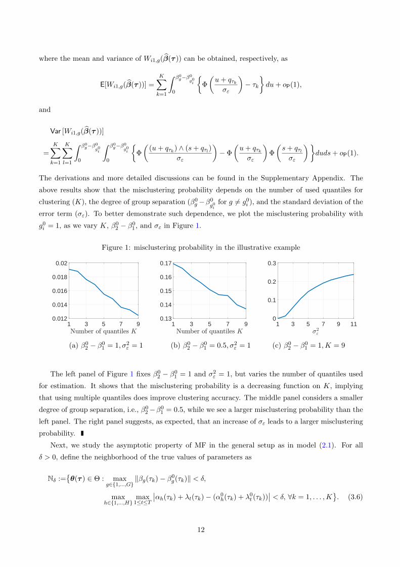
The derivations and more detailed discussions can be found in the Supplementary Appendix. The

above results show that the misclustering probability depends on the number of used quantiles for

clustering (K), the degree of group separation (β0g −β0

g0ifor g 6= g0

i ), and the standard deviation of the

error term (σε). To better demonstrate such dependence, we plot the misclustering probability with

g0i = 1, as we vary K, β0

2 − β01 , and σε in Figure 1.

Figure 1: misclustering probability in the illustrative example

1 3 5 7 90.012

0.014

0.016

0.018

0.02

1 3 5 7 90.13

0.14

0.15

0.16

0.17

1 3 5 7 9 110

0.1

0.2

0.3

(a) β02 − β0

1 = 1, σ2ε = 1 (b) β0

2 − β01 = 0.5, σ2

ε = 1 (c) β02 − β0

1 = 1,K = 9

The left panel of Figure 1 fixes β02 − β0

1 = 1 and σ2ε = 1, but varies the number of quantiles used

for estimation. It shows that the misclustering probability is a decreasing function on K, implying

that using multiple quantiles does improve clustering accuracy. The middle panel considers a smaller

degree of group separation, i.e., β02 −β0

1 = 0.5, while we see a larger misclustering probability than the

left panel. The right panel suggests, as expected, that an increase of σε leads to a larger misclustering

probability.

Next, we study the asymptotic property of MF in the general setup as in model (2.1). For all

δ > 0, define the neighborhood of the true values of parameters as

Nδ :=θ(τ ) ∈ Θ : max

g∈1,...,G‖βg(τk)− β0

g (τk)‖ < δ,

maxh∈1,...,H

max1≤t≤T

∣∣αh(τk) + λt(τk)− (α0h(τk) + λ0

t (τk))∣∣ < δ, ∀k = 1, . . . ,K

. (3.6)

12

From Corollary 1, θ(τ ) ∈ Nδ when N and T are large. Conditional on θ(τ ) ∈ Nδ, we investigate

the rate at which MF converges to 0. To this end, we introduce the mixing conditions of the strictly

stationary processes (yit − λ0t (τ), xit), t ≥ 1 for i = 1, . . . , N . Let S be a subset of 1, . . . , T and

denote σ((yit − λ0

t (τ), xit), t ∈ S)

as the sub σ-field generated from (yit − λ0t (τ), xit), t ∈ S on the

measurable space (Ω,A). For any positive integer m, define the strong and ρ-mixing coefficients of

each process as

αi(m,T ) = supn∈Z+

α(σ((yit − λ0

t (τ), xit), 1 ≤ t ≤ n), σ((yit − λ0

t (τ), xit), n+m ≤ t ≤ T)),

and

ρ∗i (m,T ) = sup∀S1,S2⊂1,...,T

mint1∈S1,t2∈S2 |t1−t2| ≥m

ρ(σ((yit − λ0

t (τ), xit), t ∈ S1

), σ((yit − λ0

t (τ), xit), t ∈ S2

)),

where α(·, ·) and ρ(·, ·) are the measures of serial dependence applied to any two sub σ-fields of A.7

Assumption 2.

(i) Denote α(m) := supi≥1

limT→∞

αi(m,T ) and ρ∗(m) := supi≥1

limT→∞

ρ∗i (m,T ). Assume that α(m) → 0 as

m→∞ and ρ∗(1) ∈ [0, 1).

(ii) For each unit i, define

Wit,gh(θ(τ )) =

K∑k=1

ρτk(yit − αh(τk)− λt(τk)− x′itβg(τk)

)− ρτk

(yit − αh0i (τk)− λt(τk)− x

′itβg0i

(τk))

.

If the process Wit,gh(θ0(τ )), t ≥ 1, with θ0(τ ) denoting the true value of θ(τ ), admits the central

limit theorem (CLT), then the following uniform convergence holds:

limT→∞

supx∈R

∣∣∣∣∣P(√

TT−1

∑Tt=1Wit,gh(θ0(τ ))− E[Wi1,gh(θ0(τ ))]√

Var [Wi1,gh(θ0(τ ))]≤ x

)− Φ(x)

∣∣∣∣∣ = 0,

where Φ is the standard normal distribution function, and the mean and variance of Wi1,gh(θ0(τ )) are

given by (A.23) and (A.28), respectively, in the Supplementary Appendix.

Assumption 2(i) requires that the process (yit − λ0t (τ), xit), t ≥ 1 is strongly mixing for each

unit. Moreover, ρ∗(1) < 1 assures that supi≥1 T−1Var [

∑Tt=1Wit,gh(θ0(τ ))] < ∞ which is needed for

the CLT of each process Wit,gh(θ0(τ )), t ≥ 1. Assumption 2(ii) strengthens pointwise convergence

to uniform convergence of the CLT, which is used to quantify the order of rate for MF (see (A.27) in

the Supplementary Appendix). When the process (yit − λ0t (τ), xit), t ≥ 1 is independent across t,

Assumption 2(ii) holds due to Berry-Esseen theorem (see Feller, 1991).

7Let A1 and A2 be any two sub σ-fields of A. The two dependence measures are given by α(A1,A2) =supA1∈A1, A2∈A2

|P(A1 ∩ A2) − P(A1)P(A2)|, and ρ(A1,A2) = supf∈L2(A1), h∈L2(A2)|Efh− EfEh| /

√Ef2Eh2, where

L2(A) denotes the space of square-integrable and A-measurable random variables.

13

The following theorem depicts the rate of convergence for MF.

Theorem 2. Suppose Assumptions 1–2 hold and log T/N → 0. For any 0 < ε < 1, there exists δ such

that conditional on θ(τ ) ∈ Nδ, as N and T →∞,

supθ(τ )∈Nδ

1− 1

N

N∑i=1

Igi = g0i , hi = h0

i = OP

(exp(−Tζ/2)

N1/2T 1/4+

exp(−Tζ)

T 1/2

), (3.7)

where

ζ =(1− ε)2

2· 1− ρ∗(1)

1 + ρ∗(1)·

infi≥1 min(g,h) 6=(gi,hi) E2[Wi1,gh(θ0(τ ))]

supi≥1 max(g,h) Var [Wi1,gh(θ0(τ ))]> 0.

This theorem shows that the MF converges to zero as N and T increase with the rate shown in

(3.7). The first term, OP

(exp(−Tζ/2)

N1/2T 1/4

), controls the rate when T 1/2 exp(Tζ) grows faster than N.

Otherwise, the second term, OP

(exp(−Tζ)T 1/2

), dominates in the rate. The exponential decrease of T

on the clustering accuracy is consistent with Bonhomme and Manresa (2015a) and Okui and Wang

(2021), both of which show the clustering accuracy improving exponentially as T increases. It also

complements Lemma 3 in Zhang et al. (2019b) by explicitly quantifying how multiple quantiles and

features of data influence the clustering accuracy. This theorem shows that the accuracy of clustering

is affected by the serial dependence of data (measured by ρ∗(1)), magnitude of the noise, number of

quantiles used for the estimation, and degree of group separation, the latter three of which appear

in the moments of Wi1,gh(θ0(τ )). More particularly, a strong serial dependence in data and a large

variance of errors impede the rate of convergence for MF, while more quantiles used for estimation

and a large degree of group separation can improve the rate.

Remark 3. The potential improvement by using multiple quantiles is, of course, conditional on a

common group structure across multiple quantiles. If certain quantiles contain no information for

clustering, incorporating these “uninformative” quantiles may lead to lower clustering accuracy than

using the most informative quantile (see also Zhang et al., 2019a). However, in practice, it is difficult to

identify the best single quantile that contains the strongest signal of clustering; therefore, the composite-

quantile-based clustering offers a robust approach that works effectively, provided that the clustering

signals across quantiles do not conflict.

The next corollary is an immediate result from Theorem 2.

Corollary 2. Under the conditions of Theorem 2, if N/(T 1/2 exp(Tε))→ 0 for all ε > 0, we obtain

P

( N⋃i=1

(gi, hi) 6= (g0

i , h0i ))→ 0

as N and T →∞, where⋃

denotes the union of events.

This corollary states the consistency of group membership estimates uniformly across all units.

Note that in addition to log T/N → 0, we require an additional growth condition of sample sizes,

namely N/(T 1/2 exp(Tε))→ 0 for all ε > 0. This condition holds when N grows polynomially in T.

14

3.3 Asymptotic distribution

Finally, we derive the asymptotic distribution of the group-specific slope coefficient estimates. First, we

show the asymptotic equivalence between the estimates obtained under the unknown and true group

memberships. Let θ(τ ) =(β(τ ), α(τ ), λ(τ )

)denote the vector of the estimated slope coefficient and

fixed effects under the true group structure. It is obtained by

θ(τ ) = arg minθ(τ )∈Θ

1

NT

N∑i=1

T∑t=1

K∑k=1

ρτk

(yit − αh0i (τk)− λt(τk)− x

′itβg0i

(τk)). (3.8)

To examine the impact of error caused by estimating latent group structures on the slope estimates,

an extra assumption is imposed.

Assumption 3. Let ωt,τk(h, g) denote the minimum eigenvalue of the following matrix:

1

N

∑i:h0i=h,g

0i=g

E[fi,τk

(αh(τk) + λt(τk)−

(α0h(τk) + λ0

t (τk))

+ x′it(βg(τk)− β0

g (τk))|xit) (

1, x′it)′ (

1, x′it)],

where h ∈ 1, . . . ,H and g ∈ 1, . . . , G. Conditional on θ(τ ) ∈ Nδ with some δ > 0,

infθ(τ )∈Nδ

inft≥1

ωt,τk(h, g)→ ωτk(h, g) > 0, and supθ(τ )∈Nδ

supt≥1

ωt,τk(h, g)→ ωτk(h, g) <∞,

for k = 1, . . . ,K.

Assumption 3 is a full rank condition, which is comparable to Assumption 1(f) in Zhang et al.

(2019a). The following corollary relates the slope coefficient estimates obtained from the unknown

and true multi-dimensional group memberships.

Corollary 3. Suppose Assumptions 1–3 hold. For k = 1, . . . ,K, we have

maxg∈1,...,G

‖βg(τk)− βg(τk)‖2 = OP

(exp(−Tζ/2)

N1/2T 1/4+

exp(−Tζ)

T 1/2

), (3.9)

as N and T →∞, where ζ is defined in Theorem 2.

This corollary states that the estimator of slope coefficients under the unknown (and estimated)

multi-dimensional group memberships converge to the infeasible estimator obtained under the true

memberships at an exponential rate of T , which further implies that the impact of the clustering

error on the coefficient estimates is limited. With the asymptotic equivalence, we can obtain the

asymptotic distribution of βg(τk) by studying that of βg(τk) for each g ∈ 1, . . . , G. We show the

Bahadur representation and asymptotic normality of βg(τk). Recall that εit(τk) = yit−Q0τk

(yit|xit) and

Fi,τk(u|x) is the conditional distribution of εi1(τk) given xi1 = x. We add extra regularity conditions

as follows.

Assumption 4.

15

(i) For each fixed i, the observations (yit, xit), t ≥ 1 are independent across t.

(ii) Let Ig := i : g0i = g. For each t, (yit − α0

h0i(τk), xit), i ∈ Ig are identically distributed

across i.

(iii) For each i, the eigenvalues of E[(1, x′i1)′(1, x′i1)] are bounded away from zero and infinity.

(iv) For each i, Fi,τk(u|x) is twice differentiable with respect to u for all x, and denote fi,τk(u|x) :=

∂Fi,τk(u|x)/∂u and f ′i,τk(u|x) := ∂fi,τk(u|x)/∂u. The following inequalities hold:

cf := sup(u,x)

fi,τk(u|x) <∞ and sup(u,x)|f ′i,τk(u|x)| <∞.

(v) There exists some constant cf < cf such that

0 < cf ≤ inft

infτ∈Tk

infxfi,τk

(α0h0i

(τ) + λ0t (τ)−

(α0h0i

(τk) + λ0t (τk)

)+ x′

(β0g0i

(τ)− β0g0i

(τk))|x),

where Tk denotes an open neighborhood of τk.

(vi) For all h ∈ 1, . . . ,H and g ∈ 1, . . . , G, limN→∞N−1∑N

i=1 Ih0i = h, g0

i = g > 0.

(vii) Let ιh,g :=∑

i:h0i=h,g0i=g E[fi,τk(0|xi1)xi1]/

∑i:h0i=h,g

0i=g fi,τk(0), and define

ΓNg :=1

N

∑h∈1,...,H

∑i:h0i=h,g

0i=g

E[fi,τk(0|xi1)xi1(x′i1 − ι′h,g)].

Assume that ΓNg is nonsingular for each N, and Γg := limN→∞ ΓNg exists and is nonsingular.

Moreover, the limit Vg := limN→∞N−1∑

h∈1,...,H∑

i:h0i=h,g0i=g E[(xi1 − ιh,g)(xi1 − ιh,g)′] exists

and is nonsingular.

Assumption 4(i), in combination with Assumption 1(i), implies that (yit, xit) are independent

across t for all i. This is needed to apply the proving strategy of Volgushev et al. (2019), such that

the variance of the remainder term of βg(τk)− β0g (τk) is controlled (see the second term on the right

side of (A.49)).8 Assumption 4(ii) requires that units from each group g are i.i.d. to make use of

some standard probability inequalities. Assumptions 4(iii)–4(v) resemble Conditions (A1)–(A3) in

Galvao et al. (2020), but are adjusted to account for multi-dimensional group structures and time

fixed effects. Assumption 4(vi) assures sufficient units in the interaction of any g and h groups, such

that the pooled estimate of αh(τk) + λt(τk) using these units, defined as

α∗h(τk) + λ∗t (τk) := arg min(α,λ)∈A×D

∑i:h0i=h,g

0i=g

ρτk(yit − (α+ λ)− x′itβ0

g (τk)),

8Since the remainder term of the representation of βg(τk) − β0g(τk) sums across t due to the presence of time fixed

effects, it is difficult to allow for the dependence across t in the asymptotic analysis here as in Galvao et al. (2020). Asour focus is mainly on the multi-dimensional clustering, we leave the analysis of asymptotic distribution in the dependentcase as future research.

16

is sufficiently close to α0h(τk) + λ0

t (τk). This condition is stronger than Assumption 1(iv) and needed

here since we follow the proving strategy of Galvao et al. (2020) to relax the growth condition of sample

sizes for asymptotic normality (see Remark 3 therein), where α∗h(τk) + λ∗t (τk) is used to approximate

the remainder term of βg(τk) − β0g (τk). We can relax this assumption at the cost of a stronger

growth condition of sample sizes (see the growth condition in Theorem 3.2 of Kato et al., 2012)

in a symmetric sense. Assumption 4(vii) guarantees the existence of the quantities needed for the

asymptotic covariance matrix of βg(τk), and is standard in the literature of panel quantile regression

(see, e.g., Condition (B3) in Kato et al., 2012).

Lemma 1. Suppose Assumptions 1 and 4 hold. If log T/N → 0 and N grows at most polynomially

in T , then for each group g, βg(τk) admits the following expansion:

βg(τk)− β0g (τk) + oP(‖βg(τk)− β0

g (τk)‖)

= Γ−1Ng

[1

NT

T∑t=1

∑h∈1,...,H

∑i:h0i=h,g

0i=g

τk − I(εit(τk) ≤ 0)(xit − ιh,g)]

+OP

(N−3/4T−1/4(logN)1/2 +N−1 logN

). (3.10)

Moreover, if T (logN)2/N → 0, then we have

√NT (βg(τk)− β0

g (τk))D−→ N(0, τk(1− τk)Γ−1

g VgΓ−1g ),

as N and T →∞.

The results in Lemma 1 are comparable to Theorem 1 of Galvao et al. (2020) for panel quantile

regressions with individual effects. As (3.8) includes the incidental parameters in the time instead

of the cross-sectional dimension, our growth condition of the sample sizes for asymptotic normality,

namely T (logN)2/N → 0, is symmetric to that of Galvao et al. (2020) by swapping the role of N

and T , and is weaker compared with those imposed in the literature of panel quantile regressions

with group heterogeneity. For example, Zhang et al. (2019a) require a much larger T than N to

achieve asymptotic normality, namely N2(logN)3/T → 0, which is a much stronger condition in the

symmetric sense. Here the restriction of the polynomial growth rate of N in T is only to simplify the

exposition of the remainder term in the Bahadur representation (3.10). The asymptotic distribution

of βg(τk) holds even without this restriction.

With Corollary 3 and Lemma 1, we can further obtain the limiting distribution of our quantile

slope estimates stated in the following theorem.

Theorem 3. Suppose Assumptions 1–4 hold. If T (logN)2/N → 0 and N grows at most polynomially

in T, we have√NT (βg(τk)− β0

g (τk))D−→ N(0, τk(1− τk)Γ−1

g VgΓ−1g ).

The asymptotic convariance matrix of βg(τk), τk(1 − τk)Γ−1g VgΓ

−1g , depends on the conditional

17

density of εit(τk). To compute this covariance matrix, one can consider estimating Γg and Vg using

a kernel approach. Specifically, let K(·) denote a kernel function, such as the normal or Epanechnikov

kernel, b = bN,T > 0 denotes the bandwidth, satisfying b→ 0 as N and T →∞, and define the scaled

kernel as Kb(z) := b−1K(z/b). Under Assumptions 1(i), 4(i) and 4(ii), for unit i such that hi = h

and gi = g, we can estimate the density function of εit(τk) at 0, fi,τk(0), by

fhg,τk =1

Nh,gT

∑i:hi=h,gi=g

T∑t=1

Kb(εit(τk)),

where Nh,g =∑N

i=1 Ihi = h, gi = g is the number of units in the h-th and g-th group, and εit(τk) =

yit − αhi(τk)− λt(τk)− x′itβgi(τk) is the estimate of εit(τk). Then we can estimate Γg and Vg by

Γg =1

NT

∑h∈1,...,H

∑i:hi=h,gi=g

T∑t=1

Kb(εit(τk))xit(xit − ιh,g)′,

Vg =1

NT

∑h∈1,...,H

∑i:hi=h,gi=g

T∑t=1

(xit − ιh,g)(xit − ιh,g)′,

where ιh,g = 1/(Nh,gT fhg,τk)∑N

i:hi=h,gi=g

∑Tt=1 Kb(εit(τk))xit. With these estimators, the kernel esti-

mator of the covariance matrix can be obtained as τk(1−τk)Γ−1g VgΓ

−1g , whose consistency follows from

the consistency of the slope and membership estimators provided in Corollaries 1 and 2.

Theorem 3 relies on large N and T , such that the estimation error of group memberships can be

ignored in β-inference owe to the superconsistency of membership estimates (see Theorem 2 and Corol-

lary 3). If one wishes to account for the misclassification error in some applications with short time

periods, a practical solution is to employ the bootstrap method, which resamples unit-specific blocks

from the original data and compute the variance using these resampled data (see, e.g., Bonhomme

and Manresa, 2015b). Numerical performance of bootstrap inference in standard quantile panel re-

gressions has been documented in Galvao and Montes-Rojas (2015), and its theoretical justifications

are recently studied in Galvao et al. (2021). It deserves future studies to investigate the theoretical

properties of bootstrapping in quantile panel regressions with latent group structures.

Remark 4. In practice, the estimated quantile regression curves may cross, violating the logical mono-

tonicity requirement. To address this problem, one can add an additional step to re-estimate the regres-

sion quantiles following the idea of Bondell et al. (2010). Specifically, with estimated group membership

hi, gi obtained from Algorithm 1, we can re-estimate αhi

(τk), λt(τk) and βgi(τk) by minimizing the

following constrained composite check function,

minθ(τ )∈Θ

1

NT

N∑i=1

T∑t=1

K∑k=1

ρτk

(yit − αhi(τk)− λt(τk)− x

′itβgi(τk)

),

s.t. αhi

(τk) + λt(τk) + x′itβgi(τk) ≥ αhi(τk−1) + λt(τk−1) + x′itβgi(τk−1) for k = 2, . . . ,K.

18

According to Bondell et al. (2010) and Corollary 3, the resulting constrained coefficient estimates are

asymptotically equivalent to the unconstrained estimates with known group memberships.

4 Determining the number of groups

Thus far, we assumed that the numbers of groups G and H are known. However, these numbers are

often unknown in applications and must be estimated. A popular approach is to minimize some infor-

mation criterion (IC) (see, e.g., Bonhomme and Manresa, 2015a; Su et al., 2016; Gu and Volgushev,

2019). Thus we consider determining the numbers of groups for the two group structures (G,H) using

the following criterion:

IC(G,H) =1

NT

K∑k=1

N∑i=1

T∑t=1

ρτk

(yit − α(G,H)

hi(τk)− λ

(G,H)t (τk)− x′itβ

(G,H)gi

(τk))

+κKnp (G,H) , (4.1)

where the superscript (G,H) refers to the estimators obtained under G and H groups for the two group

structures, np(G,H) is the total number of parameters which sums the number of group membership

parameters and quantile-specific parameters for all τk, k = 1, . . . ,K, and κ is the tuning parameter.

We decide the numbers of groups by minimizing the IC with respect to (G,H) that ranges from 1 to

some pre-specified maximum finite numbers of groups (Gmax, Hmax), respectively, namely,

(G, H) = arg min1≤G≤Gmax,1≤H≤Hmax

IC(G,H). (4.2)

To show the consistency of (G, H), we denote

σ(γg, γh) :=1

NT

K∑k=1

N∑i=1

T∑t=1

ρτk

(yit − α(G,H)

hi(τk)− λ

(G,H)t (τk)− x′itβ(G,H)

gi (τk)),

where the fixed effects and slope coefficients are estimated under some G- and H-partition (γg, γh).

Also define σ0 := plimN,T→∞1NT

∑Kk=1

∑Ni=1

∑Tt=1 ρτk

(yit − α0

h0i(τk)− λ0

t (τk)− x′itβ0g0i

(τk)), where the

superscript 0 represents the true value, and plim denotes the limit of convergence in probability.

Denote (G0, H0) as the true number of groups.

Assumption 5.

(i) plimN,T→∞min1≤G<G0 infγg∈ΓG,γh∈ΓH σ(γg, γh) > σ0 for H ≤ Hmax;

plimN,T→∞min1≤H<H0 infγg∈ΓG,γh∈ΓH σ(γg, γh) > σ0 for G ≤ Gmax.

(ii) limN,T→∞ κ = 0 and limN,T→∞√N exp(Tε) · κ ∈ (0,∞] for all ε > 0.

Assumption 5(i) requires that the value of the composite-quantile objective function of any un-

derfitted model is larger than that of the true model, and this condition in conjunction with the

first part of Assumption 5(ii) prevents underestimation of the number of groups. The second part of

Assumption 5(ii) helps to rule out the possibility of overestimating the number of groups.

19

Theorem 4. Under the conditions of Corollary 2 and Assumption 5, we have P

(G, H) = (G0, H0)→

1 as N and T →∞.

While the proposed IC works well when the group structures are common across the quantiles as

we have assumed, a word of caution here is that if the clustering signals are distinct across quantiles,

for example, strong group separation at some quantiles but very weak separation at the others, then

those quantiles with weak clustering signals may “contaminate” the behavior of the IC which is based

on the composite-quantile objective function. Such contamination may result in under-specification

of G and H in finite samples, which may further result in inconsistent slope estimates. An alternative

procedure is to first determine the optimal number of groups at each specific quantile separately based

on the quantile-specific IC (rather than the composite IC), and then choose the maximum number

over all considered quantiles. This procedure avoids contamination by quantiles with weak clustering

signals, but is more sensitive and may favor a larger numbers of groups due to the estimation noise,

especially at the tail quantiles.

5 Monte Carlo simulation

In this section, we evaluate the finite-sample performance of the proposed method. Specifically, we

examine if our method can accurately classify units and effectively recover the quantile-specific slope

coefficients within each group. We compare our approach with mean-based multi-dimensional cluster-

ing and composite-quantile one-dimensional clustering to shed light on the importance of considering

the entire distribution and multi-dimensional structures when clustering.

5.1 Data generation process

We consider four data generation processes (DGPs) that differ in the distribution of errors and the

multi-dimensional group structures.

DGP.1: We focus on the location-scale shift model:

yit = αhi + λt + βgixit + (1 + ψxit)εit, hi = 1, . . . ,H0; gi = 1, . . . , G0, (5.1)

where we set ψ = 0.5 and λt follows a standard uniform distribution, that is, U(0, 1). Following

Kato et al. (2012), we generate xit = 0.3(αhi+λt)+zit, where zit is independently and identically

generated by χ25. The error term εit is i.i.d. and follows a standard normal distribution. There are

two groups for slope coefficients (G0 = 2) but four groups for cross-section fixed effects (H0 = 4).

Each g-group contains Ng1 and Ng2 individual units, respectively, and Ng1 +Ng2 = N . We fix

the ratio among these two groups such that Ng1 : Ng2 = 0.5 : 0.5. In this DGP, we consider

that the group structure of fixed effects nests that of slopes, namely h0i = h0

j implying g0i = g0

j ,

and we fix the ratio of the number of units in the four h-groups as Nh1 : Nh2 : Nh3 : Nh4 =

20

0.25 : 0.25 : 0.25 : 0.25. In other words, the h-group structure further segments each g-group

into two equally-sized groups. The group-specific intercept and slope coefficient are set as

(α1, α2, α3, α4)′ = (−5,−2.5, 2.5, 5)′, (β1, β2)′ = (−0.75, 0.75)′.

In this case, groups are separated in their means, while the shape of their distributions is common

(see Figure 2(a) for the density function of βgi + ψεit).

DGP.2: In practice, the groups may differ not only in their means but also in their shapes

of distribution. To mimic this situation, we consider the case with heterogeneous intercepts

and slopes, and the distribution of the error term is also allowed to vary across the groups.

We generate two groups of errors following the same group structure of slope coefficients. The

first group of errors follows a standard normal distribution, while the second group follows a

Weibull distribution. By subtracting the theoretical mean, the errors of the two groups follow

heterogeneous distributions with mean zero but distinct tail behavior. In particular, we generate

εit ∼

i.i.d. N(0, 1) if gi = 1,

i.i.d. Weibull(sh, sc)− E[Weibull(sh, sc)] if gi = 2,(5.2)

where sh = 3 and sc = 1 are the shape and scale parameters of the Weibull distributions,

respectively. See Figure 2(b) for the density function of slope coefficients. Other settings remain

the same as in DGP.1.

DGP.3: This case allows the two group structures γh and γg to be non-nested. Particularly, we

generate the four h-groups by assigning the first quarter of units to Group 1, the second quarter

to Group 2, the third quarter to Group 3, and the fourth quarter to Group 4. The g-group

structure assigns the first 3/8 of units to Group 1 and the remaining to Group 2. This way

of generating memberships leads to two non-nested group structures with a smaller fraction of

overlap than those in DGP.1. Other settings remain the same as DGP.1.

DGP.4: Same as DGP.3 except that the distributions of errors are heterogeneous as in DGP.2.

For each DGP, we consider two cross-sectional sample sizes, N = (80, 160), and two lengths of

time series, T = (20, 40), leading to four combinations of cross-sectional and time series dimensions.

The number of replications is set to 1000.

5.2 Implementation and evaluation

We apply Algorithm 1 to obtain two-dimensional clustering using composite quantiles τ ∈ 0.1, 0.2,

. . . , 0.9, and refer to it as 2D-CQ. We compare it with mean-based two-dimensional clustering and

single-dimensional composite-quantile clustering estimators.

The mean-based two-dimensional clustering is an extension of the GFE estimator (Bonhomme and

Manresa, 2015a) to two-dimensional group structures, or can be viewed as a least squares version of

21

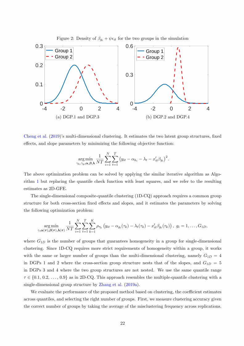
Figure 2: Density of βgi + ψεit for the two groups in the simulation

-4 -2 0 2 40

0.1

0.2

0.3 Group 1 Group 2

-4 -2 0 2 40

0.3

0.6 Group 1 Group 2

(a) DGP.1 and DGP.3 (b) DGP.2 and DGP.4

Cheng et al. (2019)’s multi-dimensional clustering. It estimates the two latent group structures, fixed

effects, and slope parameters by minimizing the following objective function:

arg minγh,γg ,α,β,λ

1

NT

N∑i=1

T∑t=1

(yit − αhi − λt − x

′itβgi

)2.

The above optimization problem can be solved by applying the similar iterative algorithm as Algo-

rithm 1 but replacing the quantile check function with least squares, and we refer to the resulting

estimates as 2D-GFE.

The single-dimensional composite-quantile clustering (1D-CQ) approach requires a common group

structure for both cross-section fixed effects and slopes, and it estimates the parameters by solving

the following optimization problem:

arg minγ,α(τ ),β(τ ),λ(τ )

1

NT

N∑i=1

T∑t=1

K∑k=1

ρτk(yit − αgi(τk)− λt(τk)− x′itβgi(τk)

), gi = 1, . . . , G1D,

where G1D is the number of groups that guarantees homogeneity in a group for single-dimensional

clustering. Since 1D-CQ requires more strict requirements of homogeneity within a group, it works

with the same or larger number of groups than the multi-dimensional clustering, namely G1D = 4

in DGPs 1 and 2 where the cross-section group structure nests that of the slopes, and G1D = 5

in DGPs 3 and 4 where the two group structures are not nested. We use the same quantile range

τ ∈ 0.1, 0.2, . . . , 0.9 as in 2D-CQ. This approach resembles the multiple-quantile clustering with a

single-dimensional group structure by Zhang et al. (2019a).

We evaluate the performance of the proposed method based on clustering, the coefficient estimates

across quantiles, and selecting the right number of groups. First, we measure clustering accuracy given

the correct number of groups by taking the average of the misclustering frequency across replications.

22

Let I(·) be the indicator function. The overall MF is computed as

MFoverall = 1− 1

N

N∑i=1

I(gi = g0i , hi = h0

i ).

We also report the MF for cross-section effects (MFH) and slope coefficients (MFG) separately, i.e.,

MFH = 1− 1

N

N∑i=1

I(hi = h0i ), and MFG = 1− 1

N

N∑i=1

I(gi = g0i ).

Second, we evaluate the accuracy of the slope coefficient estimates at each quantile, also given the

correct number of groups, based on their bias and root mean squared error (RMSE) computed, re-

spectively, as

Bias(β(τ)) =1

G

G∑g=1

[βg(τ)− β0

g (τ)], and RMSE(β(τ)) =

√√√√ 1

G

G∑g=1

[βg(τ)− β0

g (τ)]2,

where G = G0 for 2D-CQ and G = G1D for 1D-CQ. Finally, we examine how the IC-based procedure

performs in determining the number of groups. In practice, to compute the IC, we find that κ =

1.5 log(NT )/√NT works fairly well based on a large number of experiments with many alternatives,

and we employ this penalty in all simulations and the application. Our penalty term in (4.1) is

comparable to the Bayesian Information Criterion (BIC) proposed by Bonhomme and Manresa (2015b)

and Cheng et al. (2019). Performance is evaluated by the empirical probability of selecting a specific

number.9

5.3 Results

Clustering accuracy

First, we examine clustering performance. Table 1 presents the overall MF and separate MFs for

the two-dimensional groups. In general, we find that 2D-CQ produces a lower MF than 2D-GFE

and 1D-CQ in all the cases and increasing the time dimension significantly reduces the MF for all

the methods. Specifically, in DGPs 1 and 2, where the two-dimensional group structures are nested,

2D-CQ misclassifies less than 6% units when N = 80 and T = 20. Further examination reveals that

misclustering only occurs for cross-section effects but not for slope coefficients, because cross-section

effects are more difficult to estimate than slope parameters due to fewer units in h-groups (H > G)

and less variation of the unit dummy than the explanatory variable. As T increases to 40, the

MFoverall of 2D-CQ reduces to around 1%. 2D-GFE can also accurately capture slope heterogeneity

(MFG = 0) in these two DGPs, but produces higher MFH for cross-section effects than 2D-CQ. This

result suggests that employing information at multiple quantiles improves clustering when a grouped

9We also consider the alternative two-step procedure of first determining the numbers for each quantile and thenchoosing the maximum ones. The results are qualitatively similar and thus omitted here.

23

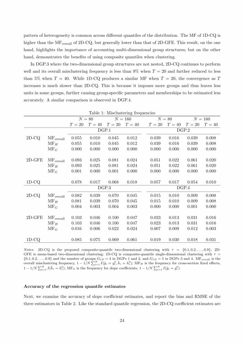
pattern of heterogeneity is common across different quantiles of the distribution. The MF of 1D-CQ is

higher than the MFoverall of 2D-CQ, but generally lower than that of 2D-GFE. This result, on the one

hand, highlights the importance of accounting multi-dimensional group structures; but on the other

hand, demonstrates the benefits of using composite quantiles when clustering.

In DGP.3 where the two-dimensional group structures are not nested, 2D-CQ continues to perform

well and its overall misclustering frequency is less than 9% when T = 20 and further reduced to less

than 5% when T = 40. While 1D-CQ produces a similar MF when T = 20, the convergence as T

increases is much slower than 2D-CQ. This is because it imposes more groups and thus leaves less

units in some groups, further causing group-specific parameters and memberships to be estimated less

accurately. A similar comparison is observed in DGP.4.

Table 1: Misclustering frequencies

N = 80 N = 160 N = 80 N = 160T = 20 T = 40 T = 20 T = 40 T = 20 T = 40 T = 20 T = 40

DGP.1 DGP.2

2D-CQ MFoverall 0.055 0.010 0.045 0.012 0.039 0.016 0.039 0.008MFH 0.055 0.010 0.045 0.012 0.039 0.016 0.039 0.008MFG 0.000 0.000 0.000 0.000 0.000 0.000 0.000 0.000

2D-GFE MFoverall 0.093 0.025 0.081 0.024 0.051 0.022 0.061 0.020MFH 0.093 0.025 0.081 0.024 0.051 0.022 0.061 0.020MFG 0.001 0.000 0.001 0.000 0.000 0.000 0.000 0.000

1D-CQ 0.078 0.017 0.068 0.018 0.057 0.017 0.054 0.010

DGP.3 DGP.4

2D-CQ MFoverall 0.082 0.039 0.070 0.045 0.015 0.010 0.009 0.008MFH 0.081 0.039 0.070 0.045 0.015 0.010 0.009 0.008MFG 0.004 0.003 0.004 0.003 0.000 0.000 0.001 0.000

2D-GFE MFoverall 0.103 0.046 0.100 0.047 0.023 0.013 0.031 0.016MFH 0.103 0.046 0.100 0.047 0.023 0.013 0.031 0.016MFG 0.016 0.006 0.022 0.024 0.007 0.009 0.012 0.003

1D-CQ 0.085 0.075 0.069 0.061 0.019 0.030 0.018 0.031

Notes: 2D-CQ is the proposed composite-quantile two-dimensional clustering with τ = 0.1, 0.2, . . . , 0.9; 2D-GFE is mean-based two-dimensional clustering; 1D-CQ is composite-quantile single-dimensional clustering with τ =0.1, 0.2, . . . , 0.9 and the number of groups G1D = 4 in DGPs 1 and 2, and G1D = 5 in DGPs 3 and 4. MFoverall is theoverall misclustering frequency, 1 − 1/N

∑Ni=1 I(gi = g0i , hi = h0

i ); MFH is the frequency for cross-section fixed effects,

1− 1/N∑Ni=1 I(hi = h0

i ); MFG is the frequency for slope coefficients, 1− 1/N∑Ni=1 I(gi = g0i ).

Accuracy of the regression quantile estimates

Next, we examine the accuracy of slope coefficient estimates, and report the bias and RMSE of the

three estimators in Table 2. Like the standard quantile regression, the 2D-CQ coefficient estimates are

24

more accurate at the central quantiles than at the tails. Comparing the 2D-CQ coefficient estimates

at the median with those of 2D-GFE, the former generally have a lower bias and RMSE due to

more accurate clustering by using composite quantiles, especially in DGP.4. The superiority of 2D-

CQ is more obvious compared with 1D-CQ, with the improvement of RMSEs as high as more than

50% in many cases. The better performance of 2D-CQ coefficient estimates is attributed to separate

estimation of the two group structures and thus more accurate clustering for slope coefficients.

Determining the number of groups

Finally, we examine how the IC-based procedure performs in determining the number of groups. We

use the IC defined in (4.1) to select the number of groups at composite quantiles τk = 0.1, 0.2, . . . , 0.9.

Table 3 provides the empirical probability of selecting specific number of groups, ranging G and H

from 1 to 6. Recall that the true number of groups is H0 = 4 and G0 = 2. The results show that

our method can effectively detect the precise number of groups in most cases and the frequency of

selecting the correct number generally increases with the time dimension.

6 Managerial incentives and risk taking

In this section, we study the economic importance of accounting for distributional heterogeneity by

revisiting the relationship between managerial incentives and risk-taking behavior. Coles et al. (2006)

examined the impact of managerial incentives on R&D expenditures scaled by total assets (RD). They

employed linear panel models with additive industry-time fixed effects and homogeneous coefficients

across firms, and found that higher sensitivity of CEO wealth to stock return volatility (vega) leads to

riskier policy choices, such as higher investment in R&D. In fact, the impact of managerial incentives

on R&D expenditure may significantly vary across different levels of expenditure, given the highly

skewed distribution of the expenditure. This effect is also likely to differ dramatically across firms

due to a heterogeneous corporate strategy, risk attitude, and managerial characteristics. Moreover,

the unobserved cross-sectional heterogeneity may not be at the industry level but more complicat-

edly depend on unobserved firm and managerial characteristics. Therefore, industry fixed effects or

industry-based grouping may not fully capture the unobserved cross-sectional heterogeneity. To cap-

ture the heterogeneous distributional effects and allow for more flexible unobserved cross-sectional

heterogeneity, we examine the same empirical question as Coles et al. (2006) using the MuGS-QR

model as:

Qτ (RDit|xit) = αhi(τ) + λt(τ) + vegait−1β1gi(τ) + deltait−1β2gi(τ) + x′itβcgi(τ), (6.1)

where lagged vega (lvega, the dollar change in the value of the CEO’s wealth for a 1% change in

standard deviation of returns) and lagged delta (ldelta, the dollar change in the value of the CEO’s

wealth for a 1% change in stock price) both measure managerial incentives, and xit contains salient

controls as in Coles et al. (2006), namely cash compensation (comp), log of sales (lsale), market-to-

25

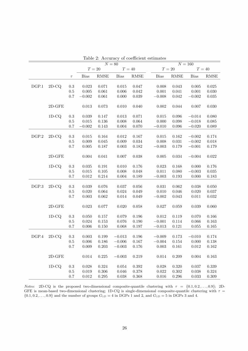
Table 2: Accuracy of coefficient estimates

N = 80 N = 160T = 20 T = 40 T = 20 T = 40

τ Bias RMSE Bias RMSE Bias RMSE Bias RMSE

DGP.1 2D-CQ 0.3 0.023 0.071 0.015 0.047 0.008 0.043 0.005 0.0250.5 0.005 0.061 0.006 0.042 0.001 0.041 0.001 0.0300.7 −0.002 0.061 0.000 0.039 −0.008 0.042 −0.002 0.035

2D-GFE 0.013 0.073 0.010 0.040 0.002 0.044 0.007 0.030

1D-CQ 0.3 0.039 0.147 0.013 0.071 0.015 0.096 −0.014 0.0800.5 0.015 0.136 0.008 0.064 0.000 0.098 −0.018 0.0850.7 −0.002 0.143 0.004 0.070 −0.010 0.096 −0.020 0.089

DGP.2 2D-CQ 0.3 0.015 0.164 0.012 0.167 0.015 0.162 −0.002 0.1740.5 0.009 0.045 0.009 0.034 0.008 0.031 −0.002 0.0180.7 0.005 0.187 0.003 0.182 −0.003 0.179 −0.001 0.179

2D-GFE 0.004 0.041 0.007 0.038 0.005 0.034 −0.004 0.022

1D-CQ 0.3 0.035 0.191 0.010 0.176 0.023 0.168 0.000 0.1760.5 0.015 0.105 0.008 0.048 0.011 0.080 −0.003 0.0350.7 0.012 0.214 0.004 0.189 −0.003 0.193 0.000 0.183

DGP.3 2D-CQ 0.3 0.039 0.076 0.037 0.056 0.031 0.062 0.038 0.0500.5 0.020 0.064 0.024 0.049 0.010 0.046 0.020 0.0370.7 0.003 0.062 0.014 0.049 −0.002 0.043 0.011 0.032

2D-GFE 0.023 0.077 0.020 0.058 0.027 0.059 0.039 0.060

1D-CQ 0.3 0.050 0.157 0.079 0.196 0.012 0.119 0.070 0.1660.5 0.024 0.153 0.076 0.190 −0.001 0.114 0.066 0.1630.7 0.006 0.150 0.068 0.197 −0.013 0.121 0.055 0.165

DGP.4 2D-CQ 0.3 0.003 0.199 −0.013 0.196 −0.009 0.173 −0.010 0.1740.5 0.006 0.186 −0.006 0.167 −0.004 0.154 0.000 0.1380.7 0.009 0.203 −0.003 0.176 0.003 0.161 0.012 0.162

2D-GFE 0.014 0.225 −0.003 0.219 0.014 0.209 0.004 0.163

1D-CQ 0.3 0.028 0.324 0.054 0.392 0.028 0.320 0.037 0.3390.5 0.019 0.306 0.046 0.378 0.022 0.302 0.038 0.3240.7 0.012 0.295 0.038 0.368 0.016 0.296 0.033 0.309

Notes: 2D-CQ is the proposed two-dimensional composite-quantile clustering with τ = 0.1, 0.2, . . . , 0.9; 2D-GFE is mean-based two-dimensional clustering; 1D-CQ is single-dimensional composite-quantile clustering with τ =0.1, 0.2, . . . , 0.9 and the number of groups G1D = 4 in DGPs 1 and 2, and G1D = 5 in DGPs 3 and 4.

26

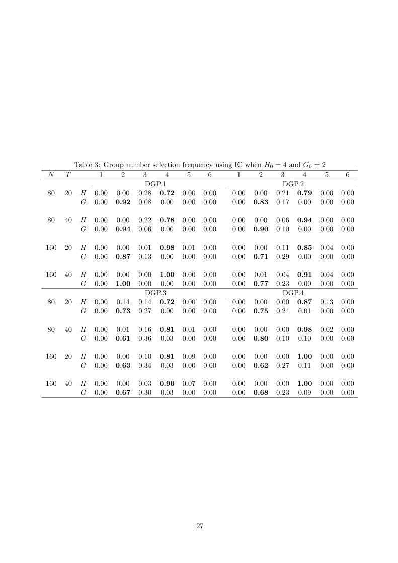
Table 3: Group number selection frequency using IC when H0 = 4 and G0 = 2

N T 1 2 3 4 5 6 1 2 3 4 5 6

DGP.1 DGP.280 20 H 0.00 0.00 0.28 0.72 0.00 0.00 0.00 0.00 0.21 0.79 0.00 0.00

G 0.00 0.92 0.08 0.00 0.00 0.00 0.00 0.83 0.17 0.00 0.00 0.00

80 40 H 0.00 0.00 0.22 0.78 0.00 0.00 0.00 0.00 0.06 0.94 0.00 0.00G 0.00 0.94 0.06 0.00 0.00 0.00 0.00 0.90 0.10 0.00 0.00 0.00

160 20 H 0.00 0.00 0.01 0.98 0.01 0.00 0.00 0.00 0.11 0.85 0.04 0.00G 0.00 0.87 0.13 0.00 0.00 0.00 0.00 0.71 0.29 0.00 0.00 0.00

160 40 H 0.00 0.00 0.00 1.00 0.00 0.00 0.00 0.01 0.04 0.91 0.04 0.00G 0.00 1.00 0.00 0.00 0.00 0.00 0.00 0.77 0.23 0.00 0.00 0.00

DGP.3 DGP.480 20 H 0.00 0.14 0.14 0.72 0.00 0.00 0.00 0.00 0.00 0.87 0.13 0.00

G 0.00 0.73 0.27 0.00 0.00 0.00 0.00 0.75 0.24 0.01 0.00 0.00

80 40 H 0.00 0.01 0.16 0.81 0.01 0.00 0.00 0.00 0.00 0.98 0.02 0.00G 0.00 0.61 0.36 0.03 0.00 0.00 0.00 0.80 0.10 0.10 0.00 0.00

160 20 H 0.00 0.00 0.10 0.81 0.09 0.00 0.00 0.00 0.00 1.00 0.00 0.00G 0.00 0.63 0.34 0.03 0.00 0.00 0.00 0.62 0.27 0.11 0.00 0.00

160 40 H 0.00 0.00 0.03 0.90 0.07 0.00 0.00 0.00 0.00 1.00 0.00 0.00G 0.00 0.67 0.30 0.03 0.00 0.00 0.00 0.68 0.23 0.09 0.00 0.00

27

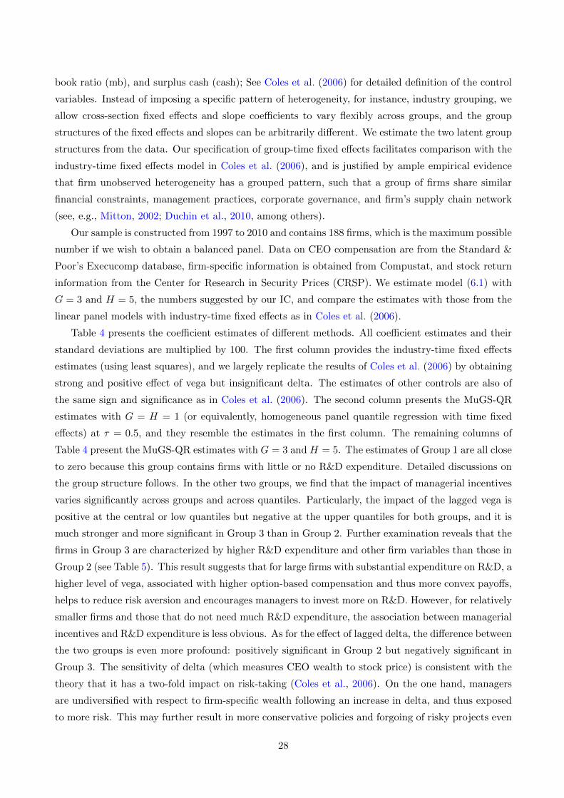
book ratio (mb), and surplus cash (cash); See Coles et al. (2006) for detailed definition of the control

variables. Instead of imposing a specific pattern of heterogeneity, for instance, industry grouping, we

allow cross-section fixed effects and slope coefficients to vary flexibly across groups, and the group

structures of the fixed effects and slopes can be arbitrarily different. We estimate the two latent group

structures from the data. Our specification of group-time fixed effects facilitates comparison with the

industry-time fixed effects model in Coles et al. (2006), and is justified by ample empirical evidence

that firm unobserved heterogeneity has a grouped pattern, such that a group of firms share similar

financial constraints, management practices, corporate governance, and firm’s supply chain network

(see, e.g., Mitton, 2002; Duchin et al., 2010, among others).

Our sample is constructed from 1997 to 2010 and contains 188 firms, which is the maximum possible

number if we wish to obtain a balanced panel. Data on CEO compensation are from the Standard &

Poor’s Execucomp database, firm-specific information is obtained from Compustat, and stock return

information from the Center for Research in Security Prices (CRSP). We estimate model (6.1) with

G = 3 and H = 5, the numbers suggested by our IC, and compare the estimates with those from the

linear panel models with industry-time fixed effects as in Coles et al. (2006).

Table 4 presents the coefficient estimates of different methods. All coefficient estimates and their

standard deviations are multiplied by 100. The first column provides the industry-time fixed effects

estimates (using least squares), and we largely replicate the results of Coles et al. (2006) by obtaining

strong and positive effect of vega but insignificant delta. The estimates of other controls are also of

the same sign and significance as in Coles et al. (2006). The second column presents the MuGS-QR

estimates with G = H = 1 (or equivalently, homogeneous panel quantile regression with time fixed

effects) at τ = 0.5, and they resemble the estimates in the first column. The remaining columns of

Table 4 present the MuGS-QR estimates with G = 3 and H = 5. The estimates of Group 1 are all close

to zero because this group contains firms with little or no R&D expenditure. Detailed discussions on

the group structure follows. In the other two groups, we find that the impact of managerial incentives

varies significantly across groups and across quantiles. Particularly, the impact of the lagged vega is

positive at the central or low quantiles but negative at the upper quantiles for both groups, and it is

much stronger and more significant in Group 3 than in Group 2. Further examination reveals that the

firms in Group 3 are characterized by higher R&D expenditure and other firm variables than those in

Group 2 (see Table 5). This result suggests that for large firms with substantial expenditure on R&D, a

higher level of vega, associated with higher option-based compensation and thus more convex payoffs,

helps to reduce risk aversion and encourages managers to invest more on R&D. However, for relatively

smaller firms and those that do not need much R&D expenditure, the association between managerial

incentives and R&D expenditure is less obvious. As for the effect of lagged delta, the difference between

the two groups is even more profound: positively significant in Group 2 but negatively significant in

Group 3. The sensitivity of delta (which measures CEO wealth to stock price) is consistent with the

theory that it has a two-fold impact on risk-taking (Coles et al., 2006). On the one hand, managers

are undiversified with respect to firm-specific wealth following an increase in delta, and thus exposed

to more risk. This may further result in more conservative policies and forgoing of risky projects even

28

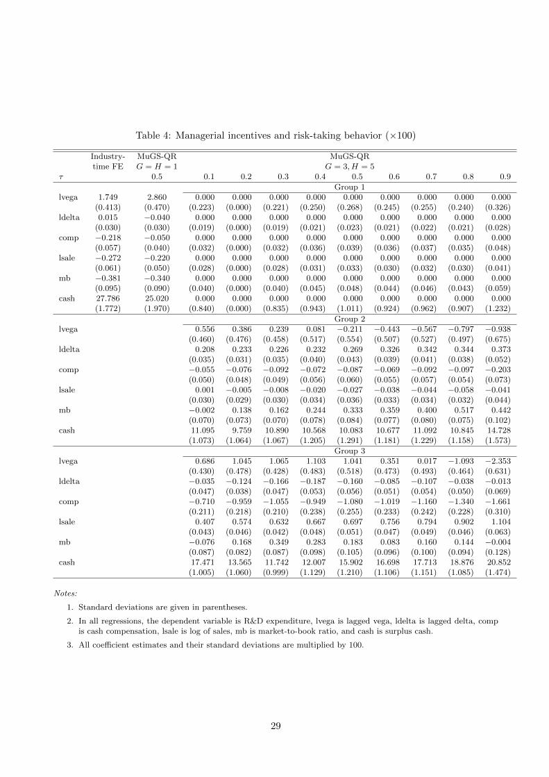
Table 4: Managerial incentives and risk-taking behavior (×100)

Industry- MuGS-QR MuGS-QRtime FE G = H = 1 G = 3, H = 5

τ 0.5 0.1 0.2 0.3 0.4 0.5 0.6 0.7 0.8 0.9

Group 1lvega 1.749 2.860 0.000 0.000 0.000 0.000 0.000 0.000 0.000 0.000 0.000

(0.413) (0.470) (0.223) (0.000) (0.221) (0.250) (0.268) (0.245) (0.255) (0.240) (0.326)ldelta 0.015 −0.040 0.000 0.000 0.000 0.000 0.000 0.000 0.000 0.000 0.000

(0.030) (0.030) (0.019) (0.000) (0.019) (0.021) (0.023) (0.021) (0.022) (0.021) (0.028)comp −0.218 −0.050 0.000 0.000 0.000 0.000 0.000 0.000 0.000 0.000 0.000

(0.057) (0.040) (0.032) (0.000) (0.032) (0.036) (0.039) (0.036) (0.037) (0.035) (0.048)lsale −0.272 −0.220 0.000 0.000 0.000 0.000 0.000 0.000 0.000 0.000 0.000

(0.061) (0.050) (0.028) (0.000) (0.028) (0.031) (0.033) (0.030) (0.032) (0.030) (0.041)mb −0.381 −0.340 0.000 0.000 0.000 0.000 0.000 0.000 0.000 0.000 0.000

(0.095) (0.090) (0.040) (0.000) (0.040) (0.045) (0.048) (0.044) (0.046) (0.043) (0.059)cash 27.786 25.020 0.000 0.000 0.000 0.000 0.000 0.000 0.000 0.000 0.000

(1.772) (1.970) (0.840) (0.000) (0.835) (0.943) (1.011) (0.924) (0.962) (0.907) (1.232)

Group 2lvega 0.556 0.386 0.239 0.081 −0.211 −0.443 −0.567 −0.797 −0.938

(0.460) (0.476) (0.458) (0.517) (0.554) (0.507) (0.527) (0.497) (0.675)ldelta 0.208 0.233 0.226 0.232 0.269 0.326 0.342 0.344 0.373

(0.035) (0.031) (0.035) (0.040) (0.043) (0.039) (0.041) (0.038) (0.052)comp −0.055 −0.076 −0.092 −0.072 −0.087 −0.069 −0.092 −0.097 −0.203

(0.050) (0.048) (0.049) (0.056) (0.060) (0.055) (0.057) (0.054) (0.073)lsale 0.001 −0.005 −0.008 −0.020 −0.027 −0.038 −0.044 −0.058 −0.041

(0.030) (0.029) (0.030) (0.034) (0.036) (0.033) (0.034) (0.032) (0.044)mb −0.002 0.138 0.162 0.244 0.333 0.359 0.400 0.517 0.442

(0.070) (0.073) (0.070) (0.078) (0.084) (0.077) (0.080) (0.075) (0.102)cash 11.095 9.759 10.890 10.568 10.083 10.677 11.092 10.845 14.728

(1.073) (1.064) (1.067) (1.205) (1.291) (1.181) (1.229) (1.158) (1.573)

Group 3lvega 0.686 1.045 1.065 1.103 1.041 0.351 0.017 −1.093 −2.353

(0.430) (0.478) (0.428) (0.483) (0.518) (0.473) (0.493) (0.464) (0.631)ldelta −0.035 −0.124 −0.166 −0.187 −0.160 −0.085 −0.107 −0.038 −0.013

(0.047) (0.038) (0.047) (0.053) (0.056) (0.051) (0.054) (0.050) (0.069)comp −0.710 −0.959 −1.055 −0.949 −1.080 −1.019 −1.160 −1.340 −1.661

(0.211) (0.218) (0.210) (0.238) (0.255) (0.233) (0.242) (0.228) (0.310)lsale 0.407 0.574 0.632 0.667 0.697 0.756 0.794 0.902 1.104

(0.043) (0.046) (0.042) (0.048) (0.051) (0.047) (0.049) (0.046) (0.063)mb −0.076 0.168 0.349 0.283 0.183 0.083 0.160 0.144 −0.004

(0.087) (0.082) (0.087) (0.098) (0.105) (0.096) (0.100) (0.094) (0.128)cash 17.471 13.565 11.742 12.007 15.902 16.698 17.713 18.876 20.852

(1.005) (1.060) (0.999) (1.129) (1.210) (1.106) (1.151) (1.085) (1.474)

Notes:

1. Standard deviations are given in parentheses.

2. In all regressions, the dependent variable is R&D expenditure, lvega is lagged vega, ldelta is lagged delta, compis cash compensation, lsale is log of sales, mb is market-to-book ratio, and cash is surplus cash.

3. All coefficient estimates and their standard deviations are multiplied by 100.

29

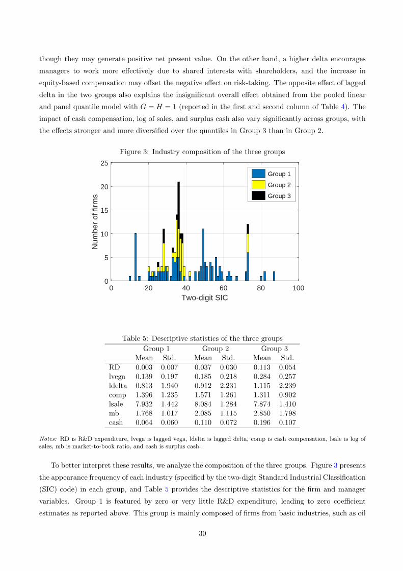
though they may generate positive net present value. On the other hand, a higher delta encourages

managers to work more effectively due to shared interests with shareholders, and the increase in

equity-based compensation may offset the negative effect on risk-taking. The opposite effect of lagged

delta in the two groups also explains the insignificant overall effect obtained from the pooled linear

and panel quantile model with G = H = 1 (reported in the first and second column of Table 4). The

impact of cash compensation, log of sales, and surplus cash also vary significantly across groups, with

the effects stronger and more diversified over the quantiles in Group 3 than in Group 2.

Figure 3: Industry composition of the three groups

0 20 40 60 80 100Two-digit SIC

0

5

10

15

20

25

Num

ber

of fi

rms

Group 1

Group 2

Group 3

Table 5: Descriptive statistics of the three groups

Group 1 Group 2 Group 3Mean Std. Mean Std. Mean Std.

RD 0.003 0.007 0.037 0.030 0.113 0.054lvega 0.139 0.197 0.185 0.218 0.284 0.257ldelta 0.813 1.940 0.912 2.231 1.115 2.239comp 1.396 1.235 1.571 1.261 1.311 0.902lsale 7.932 1.442 8.084 1.284 7.874 1.410mb 1.768 1.017 2.085 1.115 2.850 1.798cash 0.064 0.060 0.110 0.072 0.196 0.107

Notes: RD is R&D expenditure, lvega is lagged vega, ldelta is lagged delta, comp is cash compensation, lsale is log ofsales, mb is market-to-book ratio, and cash is surplus cash.

To better interpret these results, we analyze the composition of the three groups. Figure 3 presents

the appearance frequency of each industry (specified by the two-digit Standard Industrial Classification

(SIC) code) in each group, and Table 5 provides the descriptive statistics for the firm and manager

variables. Group 1 is featured by zero or very little R&D expenditure, leading to zero coefficient

estimates as reported above. This group is mainly composed of firms from basic industries, such as oil

30

& gas extraction (SIC=13), electric, gas, & sanitary services (SIC=49), and third industries (retail,

restaurants, business, etc.), which hardly require any R&D investment. Group 2 is characterized by a

moderate level of R&D and mainly contains traditional manufacturing firms specializing in chemical

& allied products (SIC=28), industrial machinery (SIC=35), transportation equipment (SIC=37),

and instruments & related products (SIC=38). Finally, firms in Group 3 are featured by high R&D

expenditure, lagged vega, market-to-book ratio, and surplus cash. The largest proportion of firms

in this group is electronic & electric (SIC=36), especially in computer-related devices (e.g., INTEL

Corp., Micron Technology Inc.) and semiconductor companies (e.g., Advanced Micro Devices, Analog

Devices). It consists of business service companies (SIC=73), but also specializes in computer-related

services, such as Electronic Arts Inc. and PTC Inc. These firms obviously require a large amount of

investment in R&D and are well valued (reflected by a high market-to-book ratio). Interestingly, the

value of vega in this group is also much higher than that of the other two groups, suggesting strong

incentives provided to managers in these firms. This confirms the strong and positive coefficient of

vega in the R&D regression at the lower and central quantiles. The negative coefficient of vega at

higher quantiles is particularly due to low vega for certain firms in 1997–1998 and around 2009 when

the Asian and global financial crises broke out, respectively.

Overall, we find a significant degree of heterogeneity in the relationship between managerial incen-

tives and risk-taking behavior across groups and in the (conditional) distribution of R&D expenditure.

The grouped pattern is to some extent related with but differs sufficiently from industry grouping,

which is often imposed by applied finance researchers. The distributional heterogeneity and the latent

group structure can be captured by our MuGS-QR model but not by the conventional two-way fixed

effects approaches.

7 Conclusion and future research

This study offers a flexible yet parsimonious way of modelling the distributional heterogeneity of

slope coefficients in panel data models with additive cross-section and time fixed effects. We model

cross-sectional heterogeneity via a latent grouped pattern and allow the group structures of cross-

section effects and slope to flexibly differ. The distributional effect within each group is captured

using regression quantiles. With the underlying assumption of quantile-invariant group memberships,

we propose a composite quantile approach to simultaneously estimate the two-dimensional group

memberships and slope parameters. We precisely quantify the convergence rate of the MF to show

that using multiple quantiles for clustering improves the accuracy of the group membership estimates

over the existing methods in which clustering is only based on the mean or some single quantile.

While two-dimensional clustering offers a flexible way of capturing heterogeneity, its resulting

estimates could be less efficient than one-dimensional clustering if the cross-section effects and slope

coefficients share a common group structure in the DGP. This is because two-dimensional clustering

estimates an unnecessarily more complex model with N extra group membership parameters. Hence,

the choice between these two clustering methods should depend on the research problem and the data.

31

As a general practical guidance, we recommend using two-dimensional clustering when T is large,

because it permits more units in a group than one-dimensional clustering and the cost of estimating

two sets of membership parameters decays quickly as T increases, as shown in Theorem 2. In a different

situation, when T is relatively small but there are sufficient cross-section units, we recommend using

one-dimensional clustering, because the misclassification error due to small T may amplify when trying

to estimate an additional set of membership parameters, while the issues of sparse interactions and

small groups associated with one-dimensional clustering may become less serious when sufficient units

are available.

Several issues deserve further research. First, we assume that group membership is invariant

across quantiles. Zhang et al. (2019a) proposed a promising clustering consensus statistic based on

perturbation techniques to verify the stability of clustering across quantiles. Alternatively, one can

test the invariance of clustering across quantiles by comparing the confidence sets of group membership

estimates proposed by Dzemski and Okui (2021) across quantiles to see if they are compatible. Second,

the computation cost is non-trivial when the number of groups is large. Thus, it is desirable to

resort to alternative algorithms that work faster and are more stable when the number of groups

is large. Third, while bootstrapping works as a practical method for inference to account for the

misclassification error, its behaviour and theoretical properties in quantile panel regressions with

latent group structures deserves future studies. Last but not the least, we assume that cross-section

fixed effects are characterized by group heterogeneity with a finite number of groups. How to estimate

a panel quantile model with individual and time fixed effects remains an open but highly challenging

topic.

Acknowledgements

We thank Serena Ng (Editor), the associate editor, anonymous referees, Mingli Chen, Ivan Fernandez-

Val, Bo Honore, Dennis Kristensen, Stepana Lazarova, Arthur Lewbel, Elena Manresa, Chris Muris,

Ryo Okui, Liangjun Su, Yixiao Sun, Yutao Sun, Stanislav Volgushev, and Martin Weidner, the par-

ticipants of seminars at the Nanyang Technological University, Erasmus University Rotterdam, Queen

Mary University of London, Maastricht University, York University, and University of Sydney, 4th

Conference of the International Society for Non-parametric Statistics in Salerno, and 4th Dongbei

Econometrics Workshop in Dalian, CMStatistics 2018 in Pisa, RES Annual Conference 2019 in War-

wick, SETA 2019 in Osaka, and ESEM 2019 in Manchester for their useful discussions and constructive

comments. Leng’s research is partially supported by the National Natural Science Foundation of China

Grant 72001183, the Fundamental Research Fund for the Central Universities 20720201047, and the

Basic Scientific Center Project 71988101 of National Science Foundation of China. Wang acknowledges

the financial support of the EUR Fellowship.

32

References

T. Ando and J. Bai. Panel data models with grouped factor structure under unknown group mem-

bership. Journal of Applied Econometrics, 31:163–191, 2016.

H. D. Bondell, B. J. Reich, and H. Wang. Noncrossing quantile regression curve estimation. Biometrika,

97:825–838, 2010.

S. Bonhomme and E. Manresa. Grouped patterns of heterogeneity in panel data. Econometrica, 83:

1147–1184, 2015a.

S. Bonhomme and E. Manresa. Supplement to ‘grouped patterns of heterogeneity in panel data’.

Econometrica Supplemental Material, 83:1147–1184, 2015b.

S. Bonhomme, T. Lamadon, and E. Manresa. Discretizing unobserved heterogeneity. Working paper,

2017.

S. Bonhomme, T. Lamadon, and E. Manresa. A distributional framework for matched employer

employee data. Econometrica, 87:699–739, 2019.

R. C. Bradley. On the spectral density and asymptotic normality of weakly dependent random fields.

Journal of Theoretical Probability, 5:355–373, 1992.

J. E. Brand and Y. Xie. Who benefits most from college? Evidence for negative selection in hetero-

geneous economic returns to higher education. American Sociological Review, 75:273–302, 2010.

M. Browning and J. Carro. Heterogeneity and microeconometrics modeling. In R. Blundell, W. Newey,

and T. Persson, editors, Advances in Economics and Econometrics, volume 3, pages 47–74. Cam-

bridge University Press, 2007.

X. Cheng, F. Schorfheide, and P. Shao. Clustering for multi-dimensional heterogeneity. Working

paper, 2019.

D. Chetverikov, B. Larsen, and C. Palmer. IV quantile regression for group-level treatments, with an

application to the distributional effects of trade. Econometrica, 84:809–833, 2016.

J. L. Coles, N. D. Daniel, and L. Naveen. Managerial incentives and risk-taking. Journal of Financial

Economics, 79:431–468, 2006.

M. Cytrynbaum. Blocked clusterwise regression. Working paper, 2020.

Y. Dong and A. Lewbel. Nonparametric identification of a binary random factor in cross section data.

Journal of Econometrics, 163:163–171, 2011.

R. Duchin, J. G. Matsusaka, and O. Ozbas. When are outside directors effective? Journal of Financial

Economics, 96:195–214, 2010.

33

A. Dzemski and R. Okui. Confidence set for group membership. Working papers, 2021.

W. Feller. An Introduction to Probability Theory and Its Applications, volume 2. John Wiley & Sons,

1991.

A. F. Galvao. Quantile regression for dynamic panel data with fixed effects. Journal of Econometrics,

164:142–157, 2011.

A. F. Galvao and K. Kato. Smoothed quantile regression for panel data. Journal of Econometrics,

193:92–112, 2016.

A. F. Galvao and G. Montes-Rojas. On bootstrap inference for quantile regression panel data: A

monte carlo study. Econometrics, 3:654–666, 2015.

A. F. Galvao, T. Juhl, G. Montes-Rojas, and J. Olmo. Testing Slope Homogeneity in Quantile

Regression Panel Data with an Application to the Cross-Section of Stock Returns. Journal of

Financial Econometrics, 16:211–243, 2017.

A. F. Galvao, J. Gu, and S. Volgushev. On the unbiased asymptotic normality of quantile regression

with fixed effects. Journal of Econometrics, 218:178–215, 2020.

A. F. Galvao, T. Parker, and Z. Xiao. Bootstrap inference for panel data quantile regression. memo,

2021.

J. Gu and S. Volgushev. Panel data quantile regression with grouped fixed effects. Journal of Econo-

metrics, 213:68–91, 2019.

J. Hahn and H. R. Moon. Panel data models with finite number of multiple equilibria. Econometric

Theory, 26:863–881, 2010.

K. Kato, A. F. Galvao, and G. V. Montes-Rojas. Asymptotics for panel quantile regression models

with individual effects. Journal of Econometrics, 170:76–91, 2012.

Y. Ke, J. Li, and W. Zhang. Structure identification in panel data analysis. The Annals of Statistics,

44:1193–1233, 2016.

K. Knight. Limiting distributions for L1 regression estimators under general conditions. The Annals

of Statistics, 26:755–770, 1998.

R. Koenker. Quantile regression for longitudinal data. Journal of Multivariate Analysis, 91:74–89,

2004.

R. Koenker. Quantile Regression. Cambridge University Press, Cambridge, UK, 2005.

E. Krasnokutskaya, K. Song, and X. Tang. Estimating unobserved agent heterogeneity using pairwise

comparisons. Journal of Econometrics, In Press, 2021.

34

C.-C. Lin and S. Ng. Estimation of panel data models with parameter heterogeneity when group

membership is unknown. Journal of Econometric Methods, 1:42–55, 2012.

R. Liu, Z. Shang, Y. Zhang, and Q. Zhou. Identification and estimation in panel models with over-

specified number of groups. Journal of Econometrics, 215:574–590, 2020.

K. Miao, L. Su, and W. Wang. Panel threshold regressions with latent group structures. Journal of

Econometrics, 214:451–481, 2020.

T. Mitton. A cross-firm analysis of the impact of corporate governance on the East Asian financial

crisis. Journal of Financial Economics, 64:215–241, 2002.

S. Ng and G. McLachlan. Mixture models for clustering multilevel growth trajectories. Computational

Statistics & Data Analysis, 71:43–51, 2014.

R. Okui and W. Wang. Heterogeneous structural breaks in panel data models. Journal of Economet-

rics, 220:447–473, 2021.

M. Peligrad. On the asymptotic normality of sequences of weak dependent random variables. Journal

of Theoretical Probability, 9:703–715, 1996.

O. Rosen, W. Jiang, and M. Tanner. Mixtures of marginal models. Biometrika, 87:391–404, 2000.

L. Su and W. Wang. Identifying latent group structures in nonlinear panels. Journal of Econometrics,

220:272–295, 2021.

L. Su, Z. Shi, and P. C. B. Phillips. Identifying latent structures in panel data. Econometrica, 84:

2215–2264, 2016.

Y. Sun. Estimation and inference in panel strcutural models. Working paper, Department of Eco-

nomics, UCSD, 2005.

M. Vogt and O. Linton. Classification of non-parametric regression functions in longitudinal data

models. Journal of the Royal Statistical Society: Series B, 79:5–27, 2016.

S. Volgushev, S.-K. Chao, G. Cheng, et al. Distributed inference for quantile regression processes.

The Annals of Statistics, 47:1634–1662, 2019.

W. Wang, P. C. B. Phillips, and L. Su. Homogeneity pursuit in panel data models: Theory and

application. Journal of Applied Econometrics, 33:797–815, 2018.

J. Yoon and A. F. Galvao. Cluster robust covariance matrix estimation in panel quantile regression

with individual fixed effects. Quantitative Economics, 11:579–608, 2020.

Y. Zhang, H. J. Wang, and Z. Zhu. Quantile-regression-based clustering for panel data. Journal of

Econometrics, 213:54–67, 2019a.

35

Y. Zhang, H. J. Wang, and Z. Zhu. Supplement to ‘quantile-regression-based clustering for panel

data’. Journal of Econometrics Supplemental Material, 213:54–67, 2019b.

E. Zwick and J. Mahon. Tax policy and heterogeneous investment behavior. American Economic

Review, 107:217–48, 2017.

36