Motion-Egomotion Discrimination and Motion Segmentation from Image-Pair Streams

Computer Vision and Image Understanding78,53–68 (2000)doi:10.1006/cviu.1999.0827, available online at http://www.idealibrary.com on

Motion–Egomotion Discrimination and MotionSegmentation from Image-Pair Streams

David Demirdjian and Radu Horaud

INRIA Rhone-Alpes and GRAVIR-CNRS, 655 Avenue de l’Europe, 38330 Montbonnot Saint Martin, FranceE-mail: [email protected]; [email protected]

Received February 19, 1999; accepted November 5, 1999

Given a sequence of image pairs we describe a method that segments the observedscene into static and moving objects while it rejects badly matched points. We showthat, using a moving stereo rig, the detection of motion can be solved in a projec-tive framework and therefore requires no camera calibration. Moreover the methodallows for articulated objects. First we establish the projective framework enablingus to characterize rigid motion in projective space. This characterization is used inconjunction with a robust estimation technique to determine egomotion. Second wedescribe a method based on data classification which further considers the non-staticscene points and groups them into several moving objects. Third we introduce astereo-tracking algorithm that provides the point-to-point correspondences neededby the algorithms. Finally we show some experiments involving a moving stereohead observing both static and moving objects.c© 2000 Academic Press

1. INTRODUCTION

The detection, description, and understanding of motion from visual data are amongthe most difficult and challenging problems in computer vision. At the low level, 3-Dmotion must be analyzed based on the 2-D appearance and time evolution features thatare observable in images. At the high level, the 2-D motion fields previously derived mustbe interpreted in terms of rigid, articulated, or deformable objects, discriminate betweenobjects undergoing distinct motions, estimate the motion parameters, etc.

If the visual sensor moves as well, one more difficulty is added because one has to estimateegomotion (the motion of the visual sensor with respect to some static reference frame) inthe same time as motion associated with the observed objects.

Existing techniques for motion/egomotion discrimination and motion segmentationroughly fall into two categories, methods using an image sequence and methods using thestereo-motion paradigm:

53

1077-3142/00 $35.00Copyright c© 2000 by Academic Press

All rights of reproduction in any form reserved.

54 DEMIRDJIAN AND HORAUD

• Image sequence analysis. These methods rely either on the estimation of the opticalflow or on point-to-point correspondences. In the former case the relationship between3-D motion of a rigid body and the observed 2-D velocities is explored. In the latter case,such constraints as the epipolar geometry and the trifocal tensor are used. Points satisfyingthe same type of constraint are assumed to belong to the same rigid object. Therefore,the problem of motion segmentation becomes the problem of grouping together pointssatisfying the same constraint [9, 13, 15, 17, 19]. For example, in [13] this grouping iscarried out by a clustering algorithm which uses a posteriori likelihood maximization.Other approaches use such techniques as the Hough transform [17] or robust estimatorswhich are used incrementally [19].• Stereo-motion analysis. These methods combine the relationship between 3-D motion

and image velocities described above with stereo constraints such as the epipolar constraintin order to disambiguate the inherent ambiguity associated with optical flow [11, 21–23].

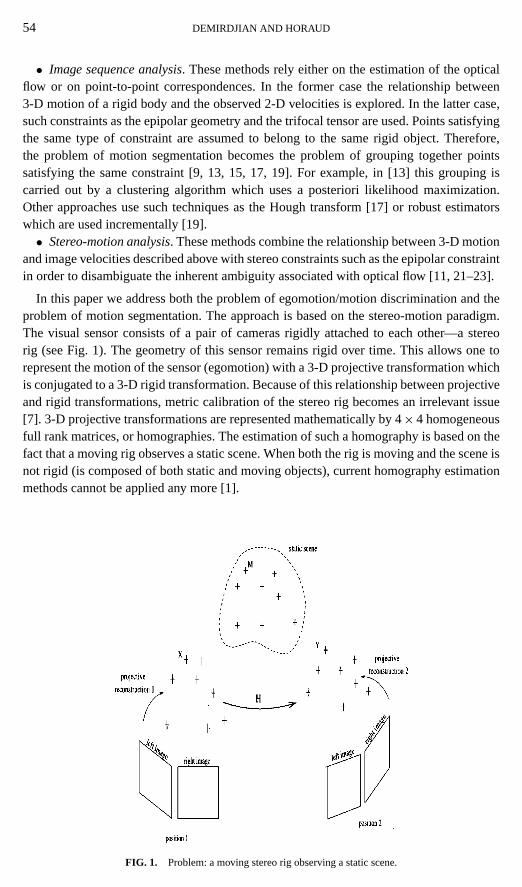
In this paper we address both the problem of egomotion/motion discrimination and theproblem of motion segmentation. The approach is based on the stereo-motion paradigm.The visual sensor consists of a pair of cameras rigidly attached to each other—a stereorig (see Fig. 1). The geometry of this sensor remains rigid over time. This allows one torepresent the motion of the sensor (egomotion) with a 3-D projective transformation whichis conjugated to a 3-D rigid transformation. Because of this relationship between projectiveand rigid transformations, metric calibration of the stereo rig becomes an irrelevant issue[7]. 3-D projective transformations are represented mathematically by 4× 4 homogeneousfull rank matrices, or homographies. The estimation of such a homography is based on thefact that a moving rig observes a static scene. When both the rig is moving and the scene isnot rigid (is composed of both static and moving objects), current homography estimationmethods cannot be applied any more [1].

FIG. 1. Problem: a moving stereo rig observing a static scene.

MOTION–EGOMOTION DISCRIMINATION 55

Therefore, the main contribution of this paper is a method for estimating 3-D projec-tive transformations associated with the sensor’s motion when the observed scene is com-posed of both static and moving objects. The output of this resolution technique consists inthe estimation of a homography associated with egomotion as well as the classification ofthe observed 2-D point correspondences into a set of inliers and a set of outliers. The inliersare compatible with the observed egomotion while the outliers are not. Therefore, the latterare farther examined by a hierarchical clustering algorithm which operated in the imageplane and over a long sequence of image pairs.

Organization

The remainder of this paper is organized as follows. The projective motion is definedin Section 2. In Section 3 we describe a robust estimator that enables to estimate theprojective motion associated with the sensor’s egomotion and the motion segmentationalgorithm is described in Section 4. The stereo tracking algorithm that provides point-to-point correspondences through a sequence of image pairs is presented in Section 5.In Section 6 we show some experiments with real data and finally the conclusions aresummarized in Section 7.

2. PROJECTIVE MOTION OF A STEREO CAMERA PAIR

Consider a 3-D pointM which is observed by a stereorig from two different positions—positionx and positiony. Let (ux, vx), (u′x, v

′x) be the image coordinates of the projections

of M when the rig is in positionx and (uy, vy) and (u′y, v′y) be the image coordinates of the

projections of the same point when the rig is in positiony. The associated homogeneouscoordinates of these points arex= (ux vx 1)>, x′ = (u′x v

′x 1)> andy= (uy vy 1)>, y′ =

(u′y v′y 1)>, wherev> denotes the transpose ofv.

Throughout this paper it is assumed that the epipolar geometry of the stereo rig is known.Since the stereo rig has a fixed geometry it is possible to associate a 3-D projective basis tothe rig and when the rig moves, this projective basisphysicallymoves with the rig. Thereforethere is a projective basis associated with each position of the rig. LetP andP′ be the 3× 4projection matrices associated with the left and right cameras. According to what has justbeen said, these matrices are fixed. The following equations hold,

{x ' PX

x′ ' P′Xand

{y ' PY

y′ ' P′Y,(1)

where “'” denotes projective equality.X and Y are 4-vectors denoting the projectivecoordinates of the physical pointM in the 3-D projective basisBx associated with positionx and the 3-D projective basisBy associated with positiony.

Equation (1) can be solved using the triangulation technique introduced by Hartley andSturm [6] and which allowsX andY to be estimated. The relationship betweenX andY is

µY=HX, (2)

whereµ is an unknown scale factor andH is a 4× 4 full-rank matrix representing a projec-tive transformation of the 3-D projective space. This matrix is defined up to a scale factor


and therefore it has 15 degrees of freedom associated with it. Equation (2) provides threelinear constraints in the entries ofH and therefore with five points in general position itis possible to solve linearly forH. However, in [1] and in [7] it was pointed out that thesolution obtained with linear resolution techniques is quite noisesensitive and at least 15to 20 points are required in order to stabilize the numerical conditioning of the associatedmeasurement matrix.

When the stereo rig has fixed geometry and undergoes rigid motion, it has been shownin [2] that the projective transformationH is conjugated to a rigid transformationD,

H ' H−1u DHu,

whereHu denotes the projective-to-metric upgrade. The above equation has been thoroughlystudied in [8, 16].H can be interpreted as a projective representation of the motion undergoneby the camera pair—projective motion—and may well be considered as an extension ofaffine motion [12] to the 3-D projective space:

DEFINITION 2.1. Consider a camera pair with known epipolar geometry which observesa 3-D rigid scene while it moves. The projective transformation between two projective re-constructions of the same 3-D scene obtained before and after the motion is called projectivemotion.

In theory, one can define projective motion without making the assumption that the stereorig has a fixed geometry. In practice, however, such an assumption is very useful. Indeed,the estimation of the epipolar geometry can be incrementally improved as new image pairsprovide new left-to-right point correspondences.

3. ROBUST ESTIMATION OF PROJECTIVE MOTION

In order to estimate projective motion one may consider Eq. (2) form ≥ 5 point corre-spondences. We obtain 3m linear equations which can be solved to determine the entries ofH. However, such a linear estimation method has two major drawbacks: (i) the method candeal neither with outliers (mismatched points) nor with nonrigid scenes (scenes that containboth static and moving objects), and (ii) the method minimizes an algebraic distance andhence it gives poor results for badly conditioned data. In particular, form= 5 the methodis very sensitive to noise [1].

To overcome these two drawbacks we introduce a new method based on robust estimationon one side and on minimizing an Euclidean error on the other side.

3.1. Robust Methods in Computer Vision

Robust regression methods are widely used to solve various vision problems such as esti-mation of epipolar geometry [18, 24] and estimation of the trifocal tensor [20]. Commonlyused robust methods are M-estimators, least-median-squares (LMedS) [14], and randomsample consensus (RANSAC) [3].

We wish to apply robust methods in order to compute projective motionH in the presenceof outliers and/or non static scenes. Moreover, we would like to deal with situations whereonly 50% of the points composing the scene belong to static objects. Therefore we mustchoose a robust method which tolerates up to 50% outliers. LMedS and RANSAC are


the only methods tolerating such a rate of outliers. At first glance they are very similar.Data subsets are selected by a random sampling process. For each such subset a solution iscomputed and a criterion must be estimated over the entire data set. The solution yieldingthe best criterion is finally kept and used in a nonlinear process to refine both the solutionand the sets of inliers/outliers. LMedS minimizes the median of the squares of the errorswhile RANSAC maximizes the number of inliers. Even if the criteria used by these twomethods are quite different, in most practical applications, comparable results are obtainedwith both methods.

The main difference between LMedS and RANSAC resides in the outlier rejection strat-egy being used. The user must supply RANSAC with a threshold value while LMedS doesnot require such a threshold. Provided that this threshold is correctly selected, this featureenables RANSAC (i) to be more efficient in the presence of nonhomogeneous noise, (ii) toallow for 50% outliers and above, and (iii) to be more efficient because it can quit therandom sampling loop as soon as a consistent solution is found. More detailed comparison/description of these algorithms can be found in [14].

In the framework of our application, the outliers may have two interpretations: they mayeither belong to independently moving objects or be “real outliers” (i.e., mismatched and/ormistracked points). As the stereo rig is observing a continuous flow of images, that meansthat the observed motions of independent objects may be small. In this case, we observethat LMedS often tends to choose an average model of all motions. As a result the set ofselected inliers often contains some points of the moving objects and the set of outlierscontains some points of the static scene.

The RANSAC algorithm performs better than LMedS in the framework of our applicationprovided that the threshold for inliers/outliers selectiontc (in the inner loop of RANSAC)is carefully chosen. As a consequence we chose this algorithm for the estimation of theprojective motionH.

The choice of the thresholdtc is crucial for the success of RANSAC and is chosen suchthat t2

c = 6.0σ 2 whereσ is the accuracy of the point location found by the stereo trackerdescribed in Section 5. This threshold is observed to be often underestimated: the correctdominant projective motion is always found (contrary to what may happen using LMedS)but some points of the static scene may not be selected as inliers. However a completionis performed at the end of RANSAC by using a thresholdt ′c slightly higher thantc (with6.0σ 2≤ t ′

2

c ≤ 9.0σ 2). Using all the successive dominant motions in a sequence and averag-ing the errors over time increases the performances of the robust algorithm (see Section 4).

Moreover the number of random samplesN must be sufficiently large to guarantee thatthe probability of selecting a good subset is high enough, say this probabilityγ must satisfyγ ≥ 0.999. The theoretical expression of this probability isγ = 1− (1− (1− εout)p)N ,wherep is the number of points that are necessary to compute a solution (p= 5 in our case)andεout is the number of outliers that are tolerated (εout= 0.5 in our case). By substitutingall these numerical values in the above formula we obtainN= 220 as the minimum numberof samples. However the expression ofγ does not take into account the presence of noiseon the inliers and a value of the order of 5 to 10 times larger than the theoretical one shouldbe used forN. Hence for the robust method to be effective, the inner loop of the algorithmmust be iterated at least 1000 times.

Moreover, remember that outliers have two physical meanings: they may well correspondeither to mismatches or to moving objects. Therefore we must be able to distinguish betweeninliers and small motions. To conclude, the estimation step in the random sampling loop


must be fast because it has to be run many times and must provide an estimation ofH asaccurate as possible.

3.2. A Quasi-linear Estimator

Let us devise an estimator forH that minimizes an Euclidean distance. In principle,such an estimator is nonlinear because of the nonlinear nature of the pinhole camera model.However, as described below, we have been able to devise a method which starts with a linearestimate ofH and which incrementally and linearly updates the Euclidean error. Therefore,this method combines the efficiency of a linear estimator with the accuracy of a nonlinearone. In practice it converges in a few iterations (2 to 3) and the solution thus obtained is veryclose to the solution that would have been obtained with a standard nonlinear minimizationmethod (see Fig. 2).

The method described below can deal with a number of point matches equal or greaterthan 5. Within the robust method described above it is however desirable to use the minimalset of points—5 points in our case.

With the notations already introduced in Sect. 2 letX be the vector of 3-D projectivecoordinates obtained by reconstruction from its projectionsx andx′ onto the first imagepair. MatrixH maps these coordinates ontoY such thatY=µHX, and matricesP andP′

reproject these coordinates onto the second image pair. Therefore we have the followingestimated image points:

α y = PHX (3)

α′ y′ = P′HX. (4)

The 3-vectorsy and y′ are defined up to a scale factor,α andα′. By dividing the first andsecond components of these vectors with their third component we get estimated imagepositions as opposed toy and y′ which are measured image positions. The Euclideandistance between the measured point positiony and the estimated point positiony is

ε2 = d2(y, y) =(

uy

ty− uy

)2

+(vy

ty− vy

)2

, (5)

with y> = (uy vy ty) andy> = (uy vy 1).Let us write matrixH ash, a vector inR16 such thath= (H11 H12 . . . H44)> = (h1 . . .

h16)>

By substituting Eq. (3) into Eq. (5) and with the notation

w = 1

ty= 1

(PHX)(3), (6)

we obtain for the Euclidean error for the left image

ε2 = w2

(16∑j=1

aj h j

)2

+ w2

(16∑j=1

bj h j

)2

, (7)


where theaj and thebj coefficients depend ony, X, andP. Since we deal with an imagepair the reprojected Euclidean error is

e2 = ε2+ ε′2. (8)

For m point matches we obtain the following criterion:

E =m∑

i=1

e2i (9)

=m∑

i=1

(w2

i

(16∑j=1

ai j h j

)2

+ w2i

(16∑j=1

bi j h j

)2

+w′2i(

16∑j=1

a′i j h j

)2

+ w′2i(

16∑j=1

b′i j h j

)2). (10)

In order to find the matrixH or, equivalently, the vectorh which minimizes the criterionE of Eq. (10) we suggest the following incremental estimation method (notice that, bydefinition, the parameterswi andw′i are dependent ofH):

1. Initialization: Letwi (0)= 1 andw′i (0)= 1. EstimateH(0) using Eq. (6).2. Evaluatethe parameterswi (k+ 1) andw′i (k+ 1) using the current solution forH(k),

i.e., Eq. (6).3. Minimize the criterionE(k+ 1) of Eq. (10) using standard weighted linear least-

squares to estimateH(k+ 1).4. Stop test: When |E(k+ 1)− E(k)|

E(k+ 1)+ E(k) <ε then stop, else return to step 2. Here we chose

ε= 10−4.

The quasi-linear estimator requires low cost computation because each iteration of theloop only involves standard weighted linear least-squares (based, in practice, on the singularvalue decomposition technique). Moreover the quasi-linear estimator generally convergesin two or three iterations.

Furthermore the quasi-linear estimator minimizes geometric error and therefore it is lessnoise-sensitive than standard linear estimators [1] and appears to be well adapted whenused in the inner loop of RANSAC: the error function associated with the inliers/outliersselection being defined by Eq. (8).

3.3. Experiments with Synthetic Data

Experiments with simulated data are carried out in order to compare the quality of theresults.

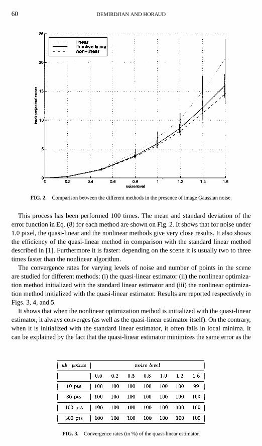
A synthetic 3-D scene consisting of 140 points is generated and placed at two differentlocations in the 3-D space. The 3-D points of each position are projected onto the camerasof a virtual stereo rig and Gaussian noise with varying standard deviation (from 0.0 to 1.6pixels) is added to the image point locations. Data are normalized as described in [5] andthree different methods are applied: the quasi-linear estimator, a standard linear method [1]and a classical nonlinear optimization method, such as Levenberg–Marquardt, initializedwith the quasi-linear estimator.


FIG. 2. Comparison between the different methods in the presence of image Gaussian noise.

This process has been performed 100 times. The mean and standard deviation of theerror function in Eq. (8) for each method are shown on Fig. 2. It shows that for noise under1.0 pixel, the quasi-linear and the nonlinear methods give very close results. It also showsthe efficiency of the quasi-linear method in comparison with the standard linear methoddescribed in [1]. Furthermore it is faster: depending on the scene it is usually two to threetimes faster than the nonlinear algorithm.

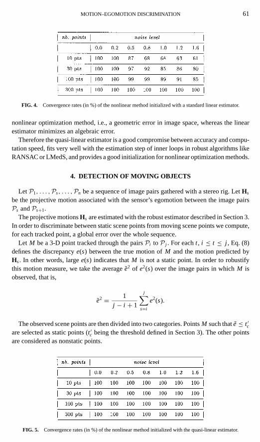
The convergence rates for varying levels of noise and number of points in the sceneare studied for different methods: (i) the quasi-linear estimator (ii) the nonlinear optimiza-tion method initialized with the standard linear estimator and (iii) the nonlinear optimiza-tion method initialized with the quasi-linear estimator. Results are reported respectively inFigs. 3, 4, and 5.

It shows that when the nonlinear optimization method is initialized with the quasi-linearestimator, it always converges (as well as the quasi-linear estimator itself). On the contrary,when it is initialized with the standard linear estimator, it often falls in local minima. Itcan be explained by the fact that the quasi-linear estimator minimizes the same error as the

FIG. 3. Convergence rates (in %) of the quasi-linear estimator.


FIG. 4. Convergence rates (in %) of the nonlinear method initialized with a standard linear estimator.

nonlinear optimization method, i.e., a geometric error in image space, whereas the linearestimator minimizes an algebraic error.

Therefore the quasi-linear estimator is a good compromise between accuracy and compu-tation speed, fits very well with the estimation step of inner loops in robust algorithms likeRANSAC or LMedS, and provides a good initialization for nonlinear optimization methods.

4. DETECTION OF MOVING OBJECTS

LetP1, . . . ,Ps, . . . ,Pn be a sequence of image pairs gathered with a stereo rig. LetHs

be the projective motion associated with the sensor’s egomotion between the image pairsPs andPs+1.

The projective motionsHs are estimated with the robust estimator described in Section 3.In order to discriminate between static scene points from moving scene points we compute,for each tracked point, a global error over the whole sequence.

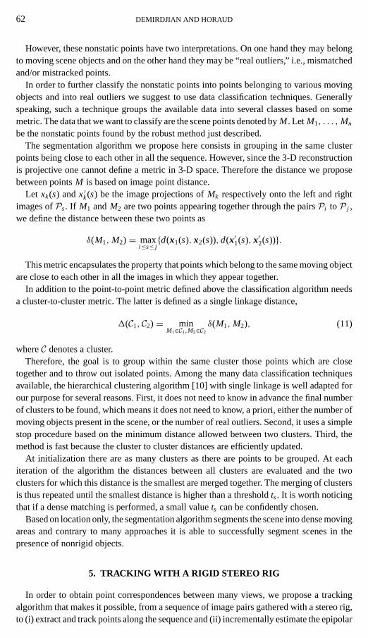
Let M be a 3-D point tracked through the pairsPi toP j . For eacht , i ≤ t ≤ j , Eq. (8)defines the discrepancye(s) between the true motion ofM and the motion predicted byHs. In other words, largee(s) indicates thatM is not a static point. In order to robustifythis motion measure, we take the averagee2 of e2(s) over the image pairs in whichM isobserved, that is,

e2 = 1

j − i + 1

j∑s=i

e2(s).

The observed scene points are then divided into two categories. PointsM such thate≤ t ′care selected as static points (t ′c being the threshold defined in Section 3). The other pointsare considered as nonstatic points.

FIG. 5. Convergence rates (in %) of the nonlinear method initialized with the quasi-linear estimator.


However, these nonstatic points have two interpretations. On one hand they may belongto moving scene objects and on the other hand they may be “real outliers,” i.e., mismatchedand/or mistracked points.

In order to further classify the nonstatic points into points belonging to various movingobjects and into real outliers we suggest to use data classification techniques. Generallyspeaking, such a technique groups the available data into several classes based on somemetric. The data that we want to classify are the scene points denoted byM . Let M1, . . . ,Mn

be the nonstatic points found by the robust method just described.The segmentation algorithm we propose here consists in grouping in the same cluster

points being close to each other in all the sequence. However, since the 3-D reconstructionis projective one cannot define a metric in 3-D space. Therefore the distance we proposebetween pointsM is based on image point distance.

Let xk(s) andx′k(s) be the image projections ofMk respectively onto the left and rightimages ofPs. If M1 andM2 are two points appearing together through the pairsPi to P j ,we define the distance between these two points as

δ(M1,M2) = maxi≤s≤ j{d(x1(s), x2(s)), d(x′1(s), x′2(s))}.

This metric encapsulates the property that points which belong to the same moving objectare close to each other in all the images in which they appear together.

In addition to the point-to-point metric defined above the classification algorithm needsa cluster-to-cluster metric. The latter is defined as a single linkage distance,

1(C1, C2) = minM1∈C1,M2∈C2

δ(M1,M2), (11)

whereC denotes a cluster.Therefore, the goal is to group within the same cluster those points which are close

together and to throw out isolated points. Among the many data classification techniquesavailable, the hierarchical clustering algorithm [10] with single linkage is well adapted forour purpose for several reasons. First, it does not need to know in advance the final numberof clusters to be found, which means it does not need to know, a priori, either the number ofmoving objects present in the scene, or the number of real outliers. Second, it uses a simplestop procedure based on the minimum distance allowed between two clusters. Third, themethod is fast because the cluster to cluster distances are efficiently updated.

At initialization there are as many clusters as there are points to be grouped. At eachiteration of the algorithm the distances between all clusters are evaluated and the twoclusters for which this distance is the smallest are merged together. The merging of clustersis thus repeated until the smallest distance is higher than a thresholdts. It is worth noticingthat if a dense matching is performed, a small valuets can be confidently chosen.

Based on location only, the segmentation algorithm segments the scene into dense movingareas and contrary to many approaches it is able to successfully segment scenes in thepresence of nonrigid objects.

5. TRACKING WITH A RIGID STEREO RIG

In order to obtain point correspondences between many views, we propose a trackingalgorithm that makes it possible, from a sequence of image pairs gathered with a stereo rig,to (i) extract and track points along the sequence and (ii) incrementally estimate the epipolar


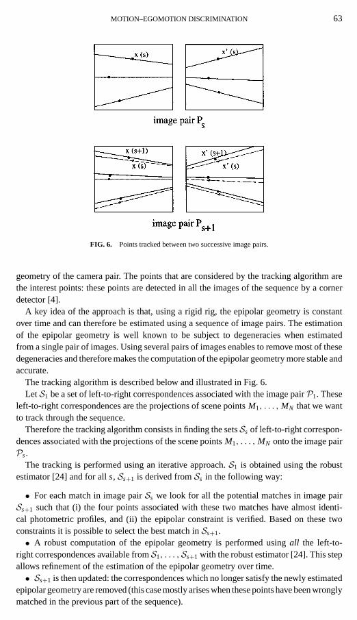
FIG. 6. Points tracked between two successive image pairs.

geometry of the camera pair. The points that are considered by the tracking algorithm arethe interest points: these points are detected in all the images of the sequence by a cornerdetector [4].

A key idea of the approach is that, using a rigid rig, the epipolar geometry is constantover time and can therefore be estimated using a sequence of image pairs. The estimationof the epipolar geometry is well known to be subject to degeneracies when estimatedfrom a single pair of images. Using several pairs of images enables to remove most of thesedegeneracies and therefore makes the computation of the epipolar geometry more stable andaccurate.

The tracking algorithm is described below and illustrated in Fig. 6.LetS1 be a set of left-to-right correspondences associated with the image pairP1. These

left-to-right correspondences are the projections of scene pointsM1, . . . ,MN that we wantto track through the sequence.

Therefore the tracking algorithm consists in finding the setsSs of left-to-right correspon-dences associated with the projections of the scene pointsM1, . . . ,MN onto the image pairPs.

The tracking is performed using an iterative approach.S1 is obtained using the robustestimator [24] and for alls, Ss+1 is derived fromSs in the following way:

• For each match in image pairSs we look for all the potential matches in image pairSs+1 such that (i) the four points associated with these two matches have almost identi-cal photometric profiles, and (ii) the epipolar constraint is verified. Based on these twoconstraints it is possible to select the best match inSs+1.• A robust computation of the epipolar geometry is performed usingall the left-to-

right correspondences available fromS1, . . . ,Ss+1 with the robust estimator [24]. This stepallows refinement of the estimation of the epipolar geometry over time.• Ss+1 is then updated: the correspondences which no longer satisfy the newly estimated

epipolar geometry are removed (this case mostly arises when these points have been wronglymatched in the previous part of the sequence).


FIG. 7. Stereo sequence 1. Each column is an image pair of the sequence.

The tracking process then goes on until the end of the sequence and enables then torobustly:

• compute the epipolar geometry of the camera pair;• match and track points between successive image pairs.

Moreover, an important feature of the tracking algorithm is that it makes possible the es-timation of the accuracy of point locationσ introduced in Section 3.1 for the computation ofthe thresholdstc andt ′c.σ is computed as the standard deviation of the errors of all the left-to-right correspondences of the sequence with respect to the epipolar geometry of the stereo rig.

6. EXPERIMENTS WITH REAL DATA

This section describes two experiments using real images. The same stereo rig has beenused for each experiment. It consists of two similar cameras. The baseline is about 30 cm andthe relative angle between optical axes is between 5.0◦ and 10.0◦ (convergent configuration).The stereo rig has been moved while capturing sequences and the following process isapplied to each sequence:

• Points are extracted and tracked with the tracking algorithm and the epipolar geometryof the stereo rig is estimated;• The projective motionsHs associated with the sensor’s egomotion are estimated;• A global errore is computed for each tracked point with respect to allHs and used for

selecting static/nonstatic points;• the segmentation of outliers into different moving objects is performed.

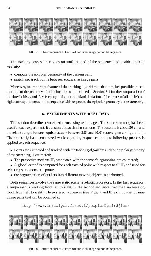
Both sequences involve the same static scene: a robotic laboratory. In the first sequence,a single man is walking from left to right. In the second sequence, two men are walking(both from left to right). These stereo sequences (see Figs. 7 and 8) each consist of nineimage pairs that can be obtained at

http://www.inrialpes.fr/movi/people/Demirdjian/

FIG. 8. Stereo sequence 2. Each column is an image pair of the sequence.


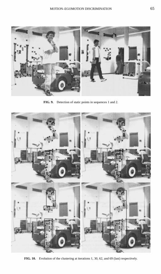
FIG. 9. Detection of static points in sequences 1 and 2.

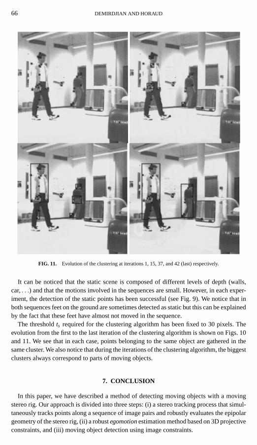
FIG. 10. Evolution of the clustering at iterations 1, 30, 62, and 69 (last) respectively.


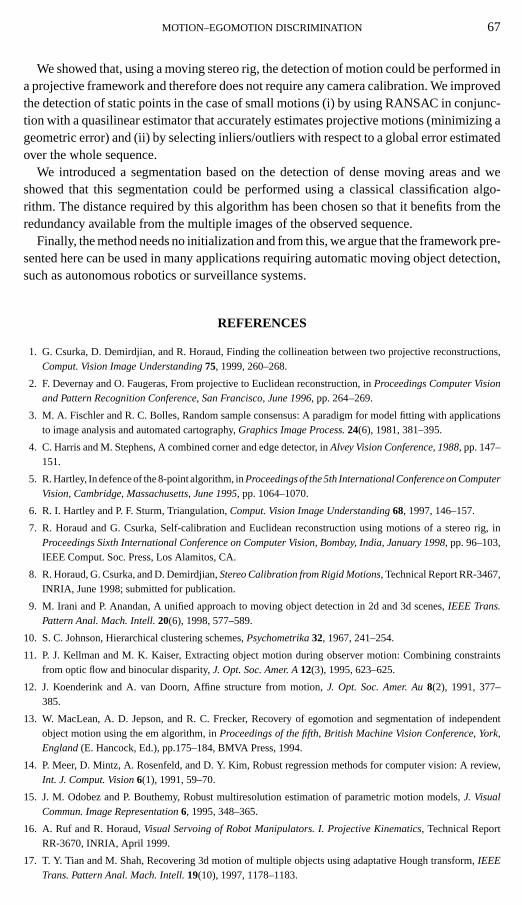
FIG. 11. Evolution of the clustering at iterations 1, 15, 37, and 42 (last) respectively.

It can be noticed that the static scene is composed of different levels of depth (walls,car,. . .) and that the motions involved in the sequences are small. However, in each exper-iment, the detection of the static points has been successful (see Fig. 9). We notice that inboth sequences feet on the ground are sometimes detected as static but this can be explainedby the fact that these feet have almost not moved in the sequence.

The thresholdts required for the clustering algorithm has been fixed to 30 pixels. Theevolution from the first to the last iteration of the clustering algorithm is shown on Figs. 10and 11. We see that in each case, points belonging to the same object are gathered in thesame cluster. We also notice that during the iterations of the clustering algorithm, the biggestclusters always correspond to parts of moving objects.

7. CONCLUSION

In this paper, we have described a method of detecting moving objects with a movingstereo rig. Our approach is divided into three steps: (i) a stereo tracking process that simul-taneously tracks points along a sequence of image pairs and robustly evaluates the epipolargeometry of the stereo rig, (ii) a robustegomotionestimation method based on 3D projectiveconstraints, and (iii) moving object detection using image constraints.


We showed that, using a moving stereo rig, the detection of motion could be performed ina projective framework and therefore does not require any camera calibration. We improvedthe detection of static points in the case of small motions (i) by using RANSAC in conjunc-tion with a quasilinear estimator that accurately estimates projective motions (minimizing ageometric error) and (ii) by selecting inliers/outliers with respect to a global error estimatedover the whole sequence.

We introduced a segmentation based on the detection of dense moving areas and weshowed that this segmentation could be performed using a classical classification algo-rithm. The distance required by this algorithm has been chosen so that it benefits from theredundancy available from the multiple images of the observed sequence.

Finally, the method needs no initialization and from this, we argue that the framework pre-sented here can be used in many applications requiring automatic moving object detection,such as autonomous robotics or surveillance systems.

REFERENCES

1. G. Csurka, D. Demirdjian, and R. Horaud, Finding the collineation between two projective reconstructions,Comput. Vision Image Understanding75, 1999, 260–268.

2. F. Devernay and O. Faugeras, From projective to Euclidean reconstruction, inProceedings Computer Visionand Pattern Recognition Conference, San Francisco, June 1996, pp. 264–269.

3. M. A. Fischler and R. C. Bolles, Random sample consensus: A paradigm for model fitting with applicationsto image analysis and automated cartography,Graphics Image Process.24(6), 1981, 381–395.

4. C. Harris and M. Stephens, A combined corner and edge detector, inAlvey Vision Conference, 1988, pp. 147–151.

5. R. Hartley, In defence of the 8-point algorithm, inProceedings of the 5th International Conference on ComputerVision, Cambridge, Massachusetts, June 1995, pp. 1064–1070.

6. R. I. Hartley and P. F. Sturm, Triangulation,Comput. Vision Image Understanding68, 1997, 146–157.

7. R. Horaud and G. Csurka, Self-calibration and Euclidean reconstruction using motions of a stereo rig, inProceedings Sixth International Conference on Computer Vision, Bombay, India, January 1998, pp. 96–103,IEEE Comput. Soc. Press, Los Alamitos, CA.

8. R. Horaud, G. Csurka, and D. Demirdjian,Stereo Calibration from Rigid Motions, Technical Report RR-3467,INRIA, June 1998; submitted for publication.

9. M. Irani and P. Anandan, A unified approach to moving object detection in 2d and 3d scenes,IEEE Trans.Pattern Anal. Mach. Intell.20(6), 1998, 577–589.

10. S. C. Johnson, Hierarchical clustering schemes,Psychometrika32, 1967, 241–254.

11. P. J. Kellman and M. K. Kaiser, Extracting object motion during observer motion: Combining constraintsfrom optic flow and binocular disparity,J. Opt. Soc. Amer. A12(3), 1995, 623–625.

12. J. Koenderink and A. van Doorn, Affine structure from motion,J. Opt. Soc. Amer. Au8(2), 1991, 377–385.

13. W. MacLean, A. D. Jepson, and R. C. Frecker, Recovery of egomotion and segmentation of independentobject motion using the em algorithm, inProceedings of the fifth, British Machine Vision Conference, York,England(E. Hancock, Ed.), pp.175–184, BMVA Press, 1994.

14. P. Meer, D. Mintz, A. Rosenfeld, and D. Y. Kim, Robust regression methods for computer vision: A review,Int. J. Comput. Vision6(1), 1991, 59–70.

15. J. M. Odobez and P. Bouthemy, Robust multiresolution estimation of parametric motion models,J. VisualCommun. Image Representation6, 1995, 348–365.

16. A. Ruf and R. Horaud,Visual Servoing of Robot Manipulators. I. Projective Kinematics, Technical ReportRR-3670, INRIA, April 1999.

17. T. Y. Tian and M. Shah, Recovering 3d motion of multiple objects using adaptative Hough transform,IEEETrans. Pattern Anal. Mach. Intell.19(10), 1997, 1178–1183.


18. P. H. S. Torr and D. W. Murray, Outlier detection and motion segmentation, inSensor Fusion VI(P. S. Schenker,Ed.), pp. 432–442, SPIE, Vol. 2059, Boston, 1993.

19. P. H. S. Torr and D. W. Murray, Stochastic motion clustering, inProceedings of the 3rd European Conferenceon Computer Vision, Stockholm, Sweden(J. O. Eklundh, Ed.), Lecture Notes in Computer Science, Vol. 801,pp. 328–337, Springer-Verlag, Berlin/New York, 1994.

20. P. H. S. Torr and A. Zisserman, Robust parameterization and computation of the trifocal tensor, inProceedingsof the Seventh British Machine Vision Conference, Edinburgh, Scotland(R. B. Fisher and E. Trucco, Eds.),Vol. 2, pp. 655–664, British Machine Vision Association, 1996.

21. W. Wang and J. H. Duncan, Recovering the three-dimensional motion and structure of multiple moving objectsfrom binocular image flows,Comput. Vision Image Understand.63, 1996, 430–446.

22. J. Weng, P. Cohen, and N. Rebibo, Motion and structure estimation from stereo image sequences,IEEE Trans.Robot. Automation8(3), 1992, 362–382.

23. J. W. Yi and J. H. Oh, Recursive resolving algorithm for multiple stereo and motion matches,Image VisionComput.15(3), 1997, 181–196.

24. Z. Zhang, R. Deriche, O. D. Faugeras, and Q.-T. Luong, A robust technique for matching two uncalibratedimages through the recovery of the unknown epipolar geometry,Artif. Intell. 78(1–2), 1995, 87–119.

Motion-Egomotion Discrimination and Motion Segmentation from Image-Pair Streams

Documents