September 25, 2002 Mortality Reductions, Educational Attainment, and Fertility Choice ∗ Abstract This paper explores the role of life expectancy as a determinant of educational attainment and fertility, both during the demographic transition and after its completion. Two main points distinguish our analysis from the previous ones. First, together with the investments of parents in the human capital of children, we introduce investments of adult individuals in their own education, which determines productivity in both the goods and household sectors. Second, we let adult longevity affect the way parents value each individual child. Increases in adult longevity eventually raise the investments in adult education. Together with the higher utility derived from each child, this tilts the quantity-quality trade off towards less and better educated children, and increases the growth rate of the economy. Reductions in child mortality may have similar effects — or may only affect fertility — depending on the nature of the costs of raising children. This setup can explain both the demographic transition and the recent behavior of fertility in “post-demographic transition” countries, ignored by the previous literature and incompatible with most of its results. Evidence from historical experiences of demographic transition, and from the recent behavior of fertility, education, and growth supports the predictions of the model. Rodrigo R. Soares Department of Economics — University of Maryland, 3105 Tydings Hall, College Park, MD, 20742; [email protected] ∗ I owe special thanks to Gary Becker, Steven Levitt, Kevin M. Murphy, and Tomas Philipson for important suggestions. I also benefited from comments from Oded Galor, Daniel Hamermesh, D. Gale Johnson, Fabian Lange, David Meltzer, Ivan Werning and seminar participants at Pompeu Fabra, EPGE—FGV, ITAM, PUC—Rio, Universidade Nova de Lisboa, University of Chicago, University of Maryland (College Park), University of Texas (Austin), and the XVIII Latin American Meeting of the Econometric Society (Buenos Aires 2001). Financial support from the Conselho Nacional de Pesquisa e Desenvolvimento Tecnológico (CNPq, Brazil) and the Esther and T. W. Schultz Endowment Fellowship (Department of Economics, University of Chicago) is gratefully acknowledged. All remaining errors are mine.

Welcome message from author
This document is posted to help you gain knowledge. Please leave a comment to let me know what you think about it! Share it to your friends and learn new things together.
Transcript
September 25, 2002
Mortality Reductions, Educational Attainment, and Fertility Choice∗
Abstract
This paper explores the role of life expectancy as a determinant of educational attainment and fertility,both during the demographic transition and after its completion. Two main points distinguish our analysisfrom the previous ones. First, together with the investments of parents in the human capital of children,we introduce investments of adult individuals in their own education, which determines productivity inboth the goods and household sectors. Second, we let adult longevity affect the way parents value eachindividual child. Increases in adult longevity eventually raise the investments in adult education. Togetherwith the higher utility derived from each child, this tilts the quantity-quality trade off towards less andbetter educated children, and increases the growth rate of the economy. Reductions in child mortalitymay have similar effects — or may only affect fertility — depending on the nature of the costs of raisingchildren. This setup can explain both the demographic transition and the recent behavior of fertility in“post-demographic transition” countries, ignored by the previous literature and incompatible with most ofits results. Evidence from historical experiences of demographic transition, and from the recent behaviorof fertility, education, and growth supports the predictions of the model.
Rodrigo R. SoaresDepartment of Economics — University of Maryland, 3105 Tydings Hall, College Park, MD, 20742;[email protected]
∗I owe special thanks to Gary Becker, Steven Levitt, Kevin M. Murphy, and Tomas Philipson for importantsuggestions. I also benefited from comments from Oded Galor, Daniel Hamermesh, D. Gale Johnson, FabianLange, David Meltzer, Ivan Werning and seminar participants at Pompeu Fabra, EPGE—FGV, ITAM, PUC—Rio,Universidade Nova de Lisboa, University of Chicago, University of Maryland (College Park), University of Texas(Austin), and the XVIII Latin American Meeting of the Econometric Society (Buenos Aires 2001). Financial supportfrom the Conselho Nacional de Pesquisa e Desenvolvimento Tecnológico (CNPq, Brazil) and the Esther and T. W.Schultz Endowment Fellowship (Department of Economics, University of Chicago) is gratefully acknowledged. Allremaining errors are mine.

1 Introduction
Major demographic changes swept the world in the course of the last century. Life expectancy
at birth rose from 40 years to around 70 years. Total fertility rates plummeted from around 6
points to close to 2 points or below. Today, over 60 countries, comprising almost 50% of the world
population, have fertility rates below replacement level (2.1), and the vast majority of people live
in countries where population is expected to stabilize within the next fifty years (Robinson and
Srinivasan, 1997). Furthermore, several developed countries have recently experienced increasingly
low fertility levels. These include Austria, Canada, Greece, Japan, and Spain, all of which have
fertility rates below 1.5. In short, recent reductions in fertility did not seem to be restricted to
experiences of demographic transition. Time and again, developed countries, believed to have
finished their transition long ago, experienced increasingly low fertility levels.
This phenomenon, largely overlooked both empirically and theoretically by the demographic
and economic literature, points to the necessity of understanding the recent behavior of fertility
from a more general perspective, not restricted to the demographic transition. The goal of this
paper is to analyze the role of life expectancy gains, determined from technical developments in
health technologies, as the driving force behind the changes in fertility, educational attainment,
and growth observed during the process of demographic transition and thereafter1 . The major
role attributed to mortality in the empirical literature on the demographic transition suggests
that life expectancy changes are indeed an independent driving force.2 This key part played
by life expectancy vis-à-vis income is further supported by the striking stability of the cross-
sectional relationship between life expectancy, fertility and schooling, as opposed to the changing
relationship between income and these same demographic variables (this evidence is discussed
in detail in Section 2). In this paper, we look at how changes in child mortality and adult
longevity affect the incentives of individuals to have children and to invest in education, and
what the consequences of these changes are to the process of economic development. Changes
in life expectancy can help explain the reductions in fertility that characterize the demographic
transition, and the changes in demographic variables that accompany economic growth.
In the last decade, extensive work has been done on the determinants of fertility, and the
relation between fertility and investments in human capital. A large part of this literature has
tried to explain the demographic transition as a consequence of increased investments in human
1 The direct welfare implications of the gains in life expectancy, and their impacts on the evolution of cross-country inequality, are discussed in Becker, Philipson and Soares (2002), and Philipson and Soares (2002).
2 See, for example, Heer and Smith (1968), Cassen (1978), Kirk (1996), Mason (1997), and Macunovich (2000).In short, the view is that “if there is a single or principal cause of fertility decline, it is reasonable to ascribe it tofalls in mortality, which was the major cause of destabilization” (Kirk, 1996, p.379).
1

capital due to technological change (Azariadis and Drazen,1990; Galor and Weil, 1996, 1999, and
2000; Hansen and Prescott, 1998; and Tamura, 1996).3 A second strand of literature analyzes
how changes in child mortality affect fertility decisions, occasionally incorporating investments of
parents in the human capital of children (Blackburn and Cipriani, 1998; Boldrin and Jones, 2002;
Ehrlich and Lui, 1991; Kalemli-Ozcan, 1999; Kalemli-Ozcan , Ryder, and Weil, 2000; Meltzer,
1992; Momota and Fugatami, 2000; and Tamura, 2001).
This paper improves upon this literature by stressing the importance of distinguishing between
child and adult mortalities, and by explicitly incorporating adult investments in human capital into
the analysis. This allows the model to addresses the recent phenomenon of small and decreasing
fertility in developed countries, ignored by the literature cited here and incompatible with most
of its results. Besides, it reveals the potential importance of adult longevity in determining the
behavior of the economy after the demographic transition.
Two specific assumptions distinguish our model from the previous ones. First, we let adult
longevity affect the way in which parents value each individual child, in much the same way that
the number of children does in the traditional fertility literature.4 This assumption is simply an
extension of the widely accepted effect of child mortality on fertility to later ages. Intuitively, it
can also be understood in these terms, once one considers that individuals are not only concerned
with the survival of their children, but also with the continuing survival of their whole lineage.
Specifically, we assume that the utility that parents derive from each child depends on the number
of children and, additionally, on the lifetime that each child will enjoy as an adult. Acknowledging
the importance of adult longevity to the way in which parents value each child has important
consequences in terms of fertility choices. This hypothesis alone helps explain the behavior of
fertility after the demographic transition.
Second, we incorporate explicitly the distinction between investments of parents’ in the human
capital of children and investments of adult individuals in their own human capital. This gener-
ates direct predictions about educational attainment and helps distinguish between the economic
3 Galor and Weil (1999) discuss briefly that reductions in mortality could increase investments in human capitaland reduce fertility via the quantity-quality trade-off.
4 The issue of fertility choice in underdeveloped economies is controversial in the demographic literature. Never-theless, evidence indicates that there is always some margin of choice. Several kinds of actions taken in ‘pre-modern’societies, directly or indirectly, affect fertility outcomes, including marriage patterns, breast feeding habits, abortion,and sexual practices (see Demeney, 1979; Caldwell, 1981; Kirk, 1996; and Mason, 1997).Also, although some individual decisions usually affect mortality, our interest here is focused on the gains in life
expectancy observed in the last two centuries, which were largely due to scientific and technical developments. Atthe individual level, these were partly exogenous. Also, these gains were exogenous to the less developed countries,which experienced mortality reductions independent of improvements in economic conditions. The gains in lifeexpectancy in less developed countries are thought to be consequence of the absorption of knowledge generatedelsewhere and of the help provided by international aid programs (see Preston, 1975 and 1980; Kirk, 1996; andBecker, Philipson, and Soares, 2001).
2
impacts of changes in adult and child mortality.5
These two features of the theory play central roles in the mechanics of the model. Briefly,
increases in adult longevity eventually raise the investments in education, which increase the
productivity of individuals both in the labor market and in the household sector. Also, higher
life expectancy tilts the quantity-quality trade-off towards less and better educated children and
tends to move the economy out of a “Malthusian” equilibrium. Once the economy abandons the
“Malthusian” regime, increases in adult longevity reduce fertility, increase educational attainment,
and increase the growth rate of the economy. Reductions in child mortality may have similar
effects, or may only affect fertility, depending on the nature of the costs of raising children.
This setup can explain the demographic transition and the recent behavior of fertility in “post-
demographic transition” countries. Besides, it reconciles theory with the evidence on the changing
relationship between income and several demographic variables.
The paper also presents different sets of evidence to support the model. Recent work suggests
that individuals’ predictions of their own life expectancies are considerably accurate, and react to
exogenous events in consistent ways (see Hamermesh, 1985; Hurd and McGarry, 1997; and Smith
et al, 2001). Therefore, the role of life expectancy in explaining changes in behavior may indeed be
empirically relevant. We argue that the exogenous role played by life expectancy in the model is
justified by the fact that recent reductions in mortality were largely independent of improvements
in economic conditions. Also, we argue that the historical experiences of demographic transition
display patterns that agree with the predictions of the model. Indeed, life expectancy gains
appear to be a driving force behind the changes observed in the other variables. Finally, we test
the predictions of the model using a cross-country panel, with data between 1960 and 1995. The
behavior of fertility, educational attainment, and growth in ‘post-transition’ economies supports
the theory. In brief, the estimated model implies that a 10 year gain in adult longevity implies
a reduction of 1.7 points in total fertility rate, an increase of 0.7 year in average schooling in the
population aged 15 and above, and a growth rate higher by 4.6%. A reduction of 100 per one
thousand in child mortality implies a reduction of 2 points in the total fertility rate.
The structure of the paper may be outlined as follows. Section 2 motivates the analysis by
presenting a very simple but striking fact: while the cross-sectional relationship between income
and some key demographic variables (life expectancy, fertility, and schooling) has been consistently
shifting in the recent past, the relationship between life expectancy and fertility and schooling has
remained considerably stable. This observation suggests that there is a dimension of changes in
5 Furthermore, this approach is more realistic and brings the theory closer to the empirical accounts that justifythe impacts of life expectancy on educational investments (see, for example, the discussion on rates of return inMeltzer, 1992).
3
life expectancy that is not explained by material development (income), but that seems to explain
changes in fertility and educational attainment. Section 3 describes the structure of the model,
and analyzes the effects of changes in adult longevity and child mortality. Section 4 discusses how
well the model describes real demographic transition histories, and tests the predictions of the
model using a cross-country panel. The final section summarizes the main results of the paper.
2 The Recent Behavior of Life Expectancy, Educational At-tainment, and Fertility
The traditional growth literature looks at income as the single variable either driving or summa-
rizing the changes in all relevant development outcomes. In this perspective, gains in per capita
income improve nutrition and health consumption, which reduces mortality rates; income gains
also change the quantity-quality trade off in terms of number and education of children, which
reduces fertility and increases human capital investment. Statements like these are common places
in the economics profession, and it seems fair to say that they give an accurate description of the
consensus regarding the main changes taking place during the process of economic development.
Even though there is a lot of truth to this view, it is far from giving a complete picture of
reality. Recently, the relationship between income and crucial demographic variables, such as life
expectancy or fertility, has been clearly unstable. Figures 1 to 3 illustrate the changing relationship
between income, life expectancy, fertility, and educational attainment.6 To concentrate on
economies that share the same demographic regime, the figures refer only to countries that had
already started the demographic transition in 1960.7
Figure 1 shows that, for constant levels of income, life expectancy has been rising.8 Logarithm
curves are fitted to the 1960 and 1995 cross sectional relation between per capita GNP and life
expectancy. For lower levels of income, life expectancy at birth has increased by more than five
years in the period between 1960 and 1995. This means, for example, that a country with per
capita GNP of US$5,000 in 1995 had a life expectancy roughly 10% higher than a country with
per capita GNP of US$5,000 in 1960.
6 The general results illustrated in Figures 1 to 5 do not depend in any way on the specific statistics used, oron the presence of any particular country in the sample. Detailed description of the variables is saved until theempirical section. The logarithm curves used are of the general form y = α + β ln(x), and the power curves usedare of the general form y = αxβ .
7 A more precise reason for the restricted sample is given in the theoretical section. Empirically, some objectivecriterion defining whether a country already started the demographic transition has inevitably to be chosen. Ourchoice is the cutoff point “countries that had life expectancy at birth above 50 years in 1960,” also to be justifiedlater on. The results do not depend on the specific criterion chosen, and there should not be much doubt regardingthe countries actually included in the sample (see Appendix).
8 This phenomenon was first noticed by Preston (1975), who analyzed data between 1930 and 1960.
4

Figure 2 tells an analogous story for the relationship between income and fertility. Again,
curves are fitted to the 1960 and 1995 cross sectional relationship between income and fertility.
For constant levels of income, fertility has been falling. These reductions have been as large as 2
points for countries with per capita income around US$3,000, and even larger for poorer countries.
Finally, as Figure 3 shows, the story is not different for the relationship between education
and income. Logarithm curves are fitted to the cross sectional relationship between income and
average schooling in 1960 and 1995. Gains in average schooling in the period were usually over 1
year, for constant levels of income.
One immediately wonders whether these changes in life expectancy, education, and fertility are
interrelated, and what the specific mechanism connecting them is. An insight in this direction is
gained by looking at the relation between life expectancy and the other two demographic variables.
In Figure 4, we plot the cross sectional relation between life expectancy and fertility in 1960
and 1995. The lines are polynomials (3rd order) fitted to the different years. At first sight, the
shift in the position of the curve suggests that a change in the relationship is being portrayed. But
if we look closely, there is not much overlapping of the two curves, and when the overlapping does
actually occur, the points relative to the different years are more or less evenly distributed over the
same area. The two segments look more like an approximation to a single stable nonlinear function
than a description of a changing relationship. This point is further explored by fitting a single
nonlinear function (3rd order polynomial) to the whole data set, assuming that a stable relation
is present throughout the period. Visually, the curve seems to have a good fit, and the functions
estimated separately for each sub-period seem to merge into it. The single fitted line actually
explains more of the overall variation in the data than the two polynomials fitted independently
to each year (R2 of 0.78, against 0.76 for 1960 and 0.21 for 1995). The interesting point is that this
curve does not separate points from 1960 and 1995 as being below or above it, as a curve fitted
to all the data in Figures 1, 2, or 3 would do. Points from the different years are distinguished
as being more on its left portion or on its right portion, as if countries were sliding on this curve
through time, via increases in life expectancy and reductions in fertility.
The results regarding life expectancy and educational attainment are even stronger. Figure
5 plots the cross sectional relationship between these two variables in 1960 and 1995, and fits a
power curve to each year. The stability of the relationship through time is clear. Indeed, the
two curves almost merge into each other for the region over which there are observations for both
years. Again, countries seem to be sliding on this curve through time, as life expectancy and
educational attainment rise simultaneously.
The figures presented illustrate that, for constant levels of income, life expectancy is rising,
5
fertility is declining, and educational attainment is increasing. At the same time, changes in
fertility and schooling are following very closely the changes in life expectancy. This has been
happening in such a way that, for a constant level of life expectancy at birth, fertility and schooling
have remained roughly constant.
In short, there is a dimension of changes in life expectancy that is not associated with income,
but that seems to be associated with changes in fertility and educational attainment. When one
thinks about these facts, one realizes that while fertility and education are direct objects of in-
dividual choice, life expectancy has a large exogenous component, related to scientific knowledge
and technological development. This reasoning suggests that exogenous reductions in mortality,
together with a stable behavioral relationship between life expectancy, educational attainment,
and fertility, may be the driving force behind the observed changes. In what follows, we de-
velop a theory along these lines. Our goal is to explain the facts discussed above, together with
the triggering of the demographic transition, as being determined by exogenous increases in life
expectancy.
3 Theory
3.1 The Structure of the Model
Assume an economy inhabited by adult individuals, who live for a deterministic amount of time,
when they work, consume, invest in their own education, have children, and invest in the education
of each child. The model is the usual ‘one sex model,’ common to the fertility literature. We
abstract from uncertainty considerations, to concentrate on the impact of adult longevity and
child mortality on the direct economic incentives at the individual level. To make the model
treatable, we also abstract from the presence of physical capital. Individuals, or households, have
an endowed level of what we call ‘basic’ human capital (determined from previous generations’
decisions), based on which they decide on how much to invest in their own ‘adult’ education.
Adult education determines productivity both in the labor market and in the household sector.
Households possess backyard technologies for producing goods, adult human capital, and basic
human capital, and they decide on how to allocate their time across these different activities in
order to maximize utility. As we will see later on, changes in adult life expectancy and child
mortality will change the incentives to engage in these different activities.
In the model, adults live for T periods, and at age τ they have children. A fraction β of the
born children dies before reaching adulthood. Parents derive utility from their own consumption
in each period of life ( c(t)σ
σ ), and from the children they have. Childhood can be thought of as an
instantaneous phase: as soon as individuals are born they become adults, and there is no decision
6

to be made as a child.
We assume that adults are concerned directly with the level of human capital of their children,
via a constant elasticity function hαcα , what is sometimes called a paternalistic approach. The
traditional literature on economics of fertility usually assumes that the value that parents place
on the human capital (or utility function) of each child is an increasing and concave function of
the number of children. Since we are incorporating longevity and child mortality into the analysis,
we also take into account the effect of these variables. We assume that, together with the number
of children, parents also care about how long each child will live, in such a way that the relevant
variable is the total lifetime of the surviving children ((1 − β)nT ), or what we call the total of
‘child-years.’ How much adults value the human capital of each child is an increasing and concave
function of the total lifetime of the children, where this function is given by ρ(.). But as a fraction
β of the children will not reach adulthood, not all of them will enjoy these T years of life. As
we treat n here as a continuous variable, we simply assume that (1− β)n out of n born children
will reach adulthood, avoiding thus the problems related to the uncertainty regarding the survival
of each individual child. Therefore, (1− β)nT assumes the role usually played by n alone in the
traditional economic analysis of fertility. Intuitively, this set up extends the logic usually applied
to child mortality rate to later ages. It is a natural extension, once one considers that individuals
are not only concerned with the survival of their children, but also with the continuing survival of
their whole lineage.9 Additionally, we assume that there is a tendency towards satiation in terms
of the total of child-years, in the sense that for sufficiently high values, its marginal utility is zero.
This seems to be a sensible hypothesis once, holding T constant, we think about the biological
constraints that nature imposes on the bearing and timing of births. It will also be important
to assure that increases in life expectancy will eventually move the economy out of a Malthusian
equilibrium.
With these hypotheses, the utility function is given by the following expression:
TZ0
exp(−θt)c(t)σ
σdt+ ρ[(1− β)nT ]
hαcα,
where θ is the subjective discount rate, and 0 < σ,α < 1; ρ0(.) > 0; ρ00(.) < 0; and ρ0(x) = 0 for
some x = x > 0. The first term denotes the utility that parents derive from their own consumption,
and the second term denotes the utility that they derive from their children.10
9 In this case, individuals take into account that their children will need enough time to have their own childrenand raise them.10 Additionally, if we assume that parents enjoy having children only to the extent that they share part of their
lifetime, the second term in the expression has to be integrated over time from τ to T , and discounted at the rate
7
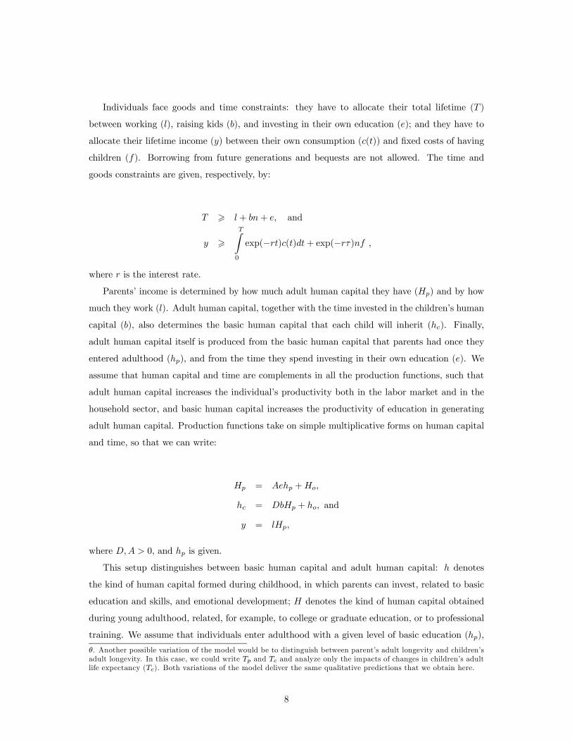
Individuals face goods and time constraints: they have to allocate their total lifetime (T )
between working (l), raising kids (b), and investing in their own education (e); and they have to
allocate their lifetime income (y) between their own consumption (c(t)) and fixed costs of having
children (f). Borrowing from future generations and bequests are not allowed. The time and
goods constraints are given, respectively, by:
T > l + bn+ e, and
y >TZ0
exp(−rt)c(t)dt+ exp(−rτ)nf ,
where r is the interest rate.
Parents’ income is determined by how much adult human capital they have (Hp) and by how
much they work (l). Adult human capital, together with the time invested in the children’s human
capital (b), also determines the basic human capital that each child will inherit (hc). Finally,
adult human capital itself is produced from the basic human capital that parents had once they
entered adulthood (hp), and from the time they spend investing in their own education (e). We
assume that human capital and time are complements in all the production functions, such that
adult human capital increases the individual’s productivity both in the labor market and in the
household sector, and basic human capital increases the productivity of education in generating
adult human capital. Production functions take on simple multiplicative forms on human capital
and time, so that we can write:
Hp = Aehp +Ho,
hc = DbHp + ho, and
y = lHp,
where D,A > 0, and hp is given.
This setup distinguishes between basic human capital and adult human capital: h denotes
the kind of human capital formed during childhood, in which parents can invest, related to basic
education and skills, and emotional development; H denotes the kind of human capital obtained
during young adulthood, related, for example, to college or graduate education, or to professional
training. We assume that individuals enter adulthood with a given level of basic education (hp),
θ. Another possible variation of the model would be to distinguish between parent’s adult longevity and children’sadult longevity. In this case, we could write Tp and Tc and analyze only the impacts of changes in children’s adultlife expectancy (Tc). Both variations of the model deliver the same qualitative predictions that we obtain here.
8
and then, by deciding on how much to invest in their own education, they choose a level of adult
human capital (Hp). hc is the level of basic human capital that parents give to each of their
children. Ho and ho denote the levels of adult and basic human capital that individuals have,
even in the absence of investments of any sort in education, maybe determined from innate skills
or natural learning throughout life. As will be clear in the following sections, these factors play
an important role in allowing for the existence of a so called Malthusian steady-state, with no
investment in human capital and zero growth.
To concentrate on the issues of interest, we depart from this formulation and introduce some
simplifying assumptions. Since our central interest is the long run behavior of the economy,
mainly the inter-generational fertility and human capital decisions, we abstract from life cycle
considerations by assuming that subjective discount rates and interest rates equal zero. Given the
separability of the utility function over time, this implies constant consumption throughout life.
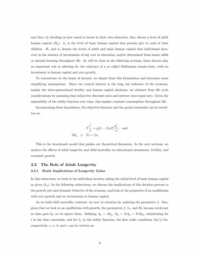
Incorporating these hypotheses, the objective function and the goods constraint can be rewrit-
ten as:
Tcσ
σ+ ρ[(1− β)nT ]
hα
c
α, and
lHp > Tc+ fn.
This is the benchmark model that guides our theoretical discussion. In the next sections, we
analyze the effects of adult longevity and child mortality on educational attainment, fertility, and
economic growth.
3.2 The Role of Adult Longevity
3.2.1 Static Implications of Longevity Gains
In this subsection, we look at the individual decision taking the initial level of basic human capital
as given (hp). In the following subsections, we discuss the implications of this decision process to
the growth rate and dynamic behavior of the economy, and look at the properties of an equilibrium
with zero growth and no investments in human capital.
As we hold child mortality constant, we save in notation by omitting the parameter β. Also,
given that we look at an equilibrium with growth, the parameters f , ho, and Ho become irrelevant
as time goes by, so we ignore them. Defining Ap = Ahp, Dp = DAp = DAhp, substituting for
l in the time constraint, and for hc in the utility function, the first order conditions (foc’s) for,
respectively, c, n, b, and e can be written as:
9
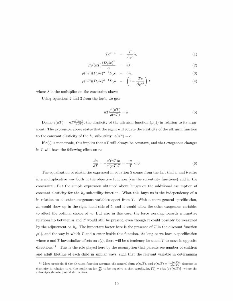
Tcσ−1 =T
Apeλ, (1)
Tρ0(nT )(Dpbe)
α
α= bλ, (2)
ρ(nT )(Dpbe)α−1Dpe = nλ, (3)
ρ(nT )(Dpbe)α−1Dpb =
µ1− Tc
Ape2
¶λ; (4)
where λ is the multiplier on the constraint above.
Using equations 2 and 3 from the foc’s, we get:
nTρ0(nT )ρ(nT )
= α. (5)
Define ε(nT ) = nT ρ0(nT )ρ(nT ) , the elasticity of the altruism function (ρ(.)) in relation to its argu-
ment. The expression above states that the agent will equate the elasticity of the altruism function
to the constant elasticity of the hc sub-utility: ε(nT ) = α.
If ε(.) is monotonic, this implies that nT will always be constant, and that exogenous changes
in T will have the following effect on n:
dn
dT= − ε0(nT )n
ε0(nT )T= −n
T< 0. (6)
The equalization of elasticities expressed in equation 5 comes from the fact that n and b enter
in a multiplicative way both in the objective function (via the sub-utility functions) and in the
constraint. But the simple expression obtained above hinges on the additional assumption of
constant elasticity for the hc sub-utility function. What this buys us is the independency of n
in relation to all other exogenous variables apart from T . With a more general specification,
hc would show up in the right hand side of 5, and it would allow the other exogenous variables
to affect the optimal choice of n. But also in this case, the force working towards a negative
relationship between n and T would still be present, even though it could possibly be weakened
by the adjustment on hc. The important factor here is the presence of T in the discount function
ρ(.), and the way in which T and n enter inside this function. As long as we have a specification
where n and T have similar effects on ε(.), there will be a tendency for n and T to move in opposite
directions.11 This is the role played here by the assumption that parents see number of children
and adult lifetime of each child in similar ways, such that the relevant variable in determining
11 More precisely, if the altruism function assumes the general form ρ(n, T ), and ε(n, T ) =ρn(n,T )nρ(n,T )
denotes its
elasticity in relation to n, the condition for dndT
to be negative is that sign{εn(n, T )} = sign{εT (n, T )}, where thesubscripts denote partial derivatives.
10
how much parents care for each individual child is the total lifetime of the children, or the total
of ‘child-years.’
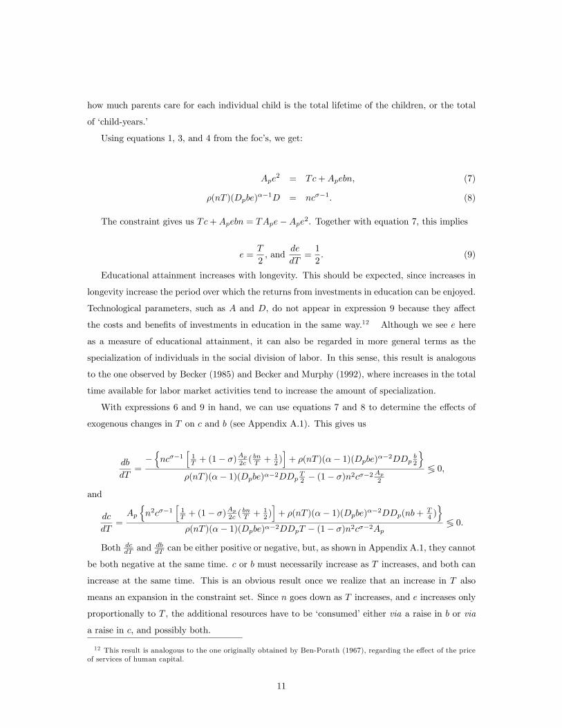
Using equations 1, 3, and 4 from the foc’s, we get:
Ape2 = Tc+Apebn, (7)
ρ(nT )(Dpbe)α−1D = ncσ−1. (8)
The constraint gives us Tc+Apebn = TApe−Ape2. Together with equation 7, this implies
e =T
2, and
de
dT=1
2. (9)
Educational attainment increases with longevity. This should be expected, since increases in
longevity increase the period over which the returns from investments in education can be enjoyed.
Technological parameters, such as A and D, do not appear in expression 9 because they affect
the costs and benefits of investments in education in the same way.12 Although we see e here
as a measure of educational attainment, it can also be regarded in more general terms as the
specialization of individuals in the social division of labor. In this sense, this result is analogous
to the one observed by Becker (1985) and Becker and Murphy (1992), where increases in the total
time available for labor market activities tend to increase the amount of specialization.
With expressions 6 and 9 in hand, we can use equations 7 and 8 to determine the effects of
exogenous changes in T on c and b (see Appendix A.1). This gives us
db
dT=−nncσ−1
h1T + (1− σ)
Ap2c (
bnT +
12)i+ ρ(nT )(α− 1)(Dpbe)α−2DDp b2
oρ(nT )(α− 1)(Dpbe)α−2DDp T2 − (1− σ)n2cσ−2Ap2
≶ 0,
and
dc
dT=Ap
nn2cσ−1
h1T + (1− σ)
Ap2c (
bnT +
12)i+ ρ(nT )(α− 1)(Dpbe)α−2DDp(nb+ T
4 )o
ρ(nT )(α− 1)(Dpbe)α−2DDpT − (1− σ)n2cσ−2Ap≶ 0.
Both dcdT and
dbdT can be either positive or negative, but, as shown in Appendix A.1, they cannot
be both negative at the same time. c or b must necessarily increase as T increases, and both can
increase at the same time. This is an obvious result once we realize that an increase in T also
means an expansion in the constraint set. Since n goes down as T increases, and e increases only
proportionally to T , the additional resources have to be ‘consumed’ either via a raise in b or via
a raise in c, and possibly both.
12 This result is analogous to the one originally obtained by Ben-Porath (1967), regarding the effect of the priceof services of human capital.
11

The specific signs of dcdT and db
dT depend on the values of the parameters, but the forces at
work can be understood by looking at the individual problem. We know that, as T increases, the
shadow price of the time b invested in hc (n) goes down, and the productivity of this investment
goes up (e), so that hc must increase in the new optimum, even though b itself may decrease.
Depending on the magnitude of the decrease in this shadow price, and on the concavity of the
sub-utility functions (σ and α), it will be worthwhile for the individual also to increase c together
with hc, or to let c decrease as hc increases.
It is easy to show that hc unequivocally increases as T increases. Since hc = Dpbe, we have
that dhcdT = Dp(bdedT + e
dbdT ), which gives:
dhcdT
=−Dp
©2cσ−1n
£1 + (1− σ) bnc Ap
¤+ (1− σ)ncσ−2Ap T2
ªρ(nT )(α− 1)(Dpbe)α−2DDpT + (σ − 1)n2cσ−2Ap > 0.
It may seem counter-intuitive that cmay actually go down as T increases, but it is important to
keep in mind exactly what this theoretical experiment corresponds to. Here, we are analyzing an
increase in T holding constant the level of basic human capital of parents (hp). So, the result means
that individuals entering adulthood that face an increase in their life expectancy will increase their
own education and the basic education that they give to their children. And it may even be the
case that they reduce their own consumption in each period in order to be able to invest more in
the children’s human capital. This is different from analyzing what will be the effect of T on the
consumption pattern across generations. As we will see now, the model predicts that increases in
T increase the growth rate of consumption across generations.
3.2.2 Dynamic Implications of Longevity Gains
In order for a steady-state to exist in this economy, preferences have to be homothetic over c and
hc. This guarantees that, as the economy grows, individuals from different generations will make
optimal decisions such that c and hp will grow at the same constant rate, and b, n, e, and l will
be constant. In our set up, this is equivalent to imposing the condition σ = α.13
Assuming that this condition holds, the production function of hc implies that the growth rate
of basic human capital is given by14 (1 + γ) = hchp= DAbe. From the goods constraint, we have
that Ahple = Tc, which implies that, in steady-state, c will grow at the same rate of hp, namely,
(1+γ). The same will also be true for the level of adult human capital (Hp), as can be seen from
the production function Hp = Aehp.
13 The existence of a steady-state is not essential. Nevertheless, it greatly simplifies the discussion. A formalanalysis of the codition σ = α and of the consequences of deviating from this assumption is contained in AppendixA.2.14 If DAbe < 1, there is no growth in steady-state. In this case, Ho and ho will be important in determining the
human capital and consumption levels in equilibrium.
12
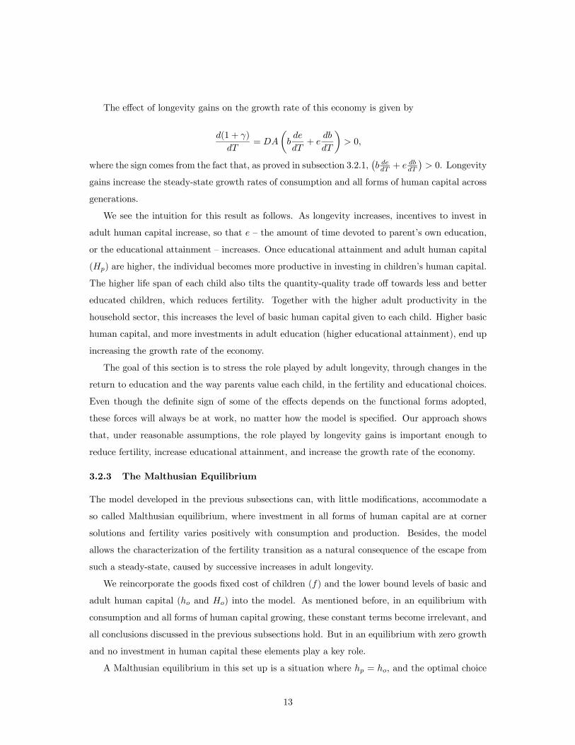
The effect of longevity gains on the growth rate of this economy is given by
d(1 + γ)
dT= DA
µbde
dT+ e
db
dT
¶> 0,
where the sign comes from the fact that, as proved in subsection 3.2.1,¡b dedT + e
dbdT
¢> 0. Longevity
gains increase the steady-state growth rates of consumption and all forms of human capital across
generations.
We see the intuition for this result as follows. As longevity increases, incentives to invest in
adult human capital increase, so that e — the amount of time devoted to parent’s own education,
or the educational attainment — increases. Once educational attainment and adult human capital
(Hp) are higher, the individual becomes more productive in investing in children’s human capital.
The higher life span of each child also tilts the quantity-quality trade off towards less and better
educated children, which reduces fertility. Together with the higher adult productivity in the
household sector, this increases the level of basic human capital given to each child. Higher basic
human capital, and more investments in adult education (higher educational attainment), end up
increasing the growth rate of the economy.
The goal of this section is to stress the role played by adult longevity, through changes in the
return to education and the way parents value each child, in the fertility and educational choices.
Even though the definite sign of some of the effects depends on the functional forms adopted,
these forces will always be at work, no matter how the model is specified. Our approach shows
that, under reasonable assumptions, the role played by longevity gains is important enough to
reduce fertility, increase educational attainment, and increase the growth rate of the economy.
3.2.3 The Malthusian Equilibrium
The model developed in the previous subsections can, with little modifications, accommodate a
so called Malthusian equilibrium, where investment in all forms of human capital are at corner
solutions and fertility varies positively with consumption and production. Besides, the model
allows the characterization of the fertility transition as a natural consequence of the escape from
such a steady-state, caused by successive increases in adult longevity.
We reincorporate the goods fixed cost of children (f) and the lower bound levels of basic and
adult human capital (ho and Ho) into the model. As mentioned before, in an equilibrium with
consumption and all forms of human capital growing, these constant terms become irrelevant, and
all conclusions discussed in the previous subsections hold. But in an equilibrium with zero growth
and no investment in human capital these elements play a key role.
A Malthusian equilibrium in this set up is a situation where hp = ho, and the optimal choice
13

of the individual implies b = e = 0. Collapsing all the constraints into only one and writing the
problem in terms of {c, n, b, e}, this equilibrium is characterized by the following foc’s, where λ is
still the multiplier on the constraint:
cσ−1 =λ
Ho,
Tρ0(nT )ho
α
α=
f
Hoλ,
ρ(nT )hα−1o DHo < nλ,
0 <
·1− Aho(Tc+ fn)
H2o
¸λ.
We call this corner solution a Malthusian equilibrium because, in a situation like this, changes
in productivity — brought about, for example, by exogenous changes in Ho — will be positively
correlated with changes in both consumption and fertility (for proof and further discussion, see
Appendix A.3).
While this corner solution holds, changes in T will only be associated with changes in c and
n. Working with the first two foc’s and the constraint, we get the effects of T on c and n:
dn
dT=
f2nT2 (σ − 1)cσ−2 − h
α
o
α [nTρ00(nT ) + ρ0(nT )]
T 2ρ00(nT )hαo
α + f2
T (σ − 1)cσ−2≶ 0, and
dc
dT=
fhα
o
α [2nTρ00(nT ) + ρ0(nT )]
T 3ρ00(nT )hαo
α + f2(σ − 1)cσ−2≷ 0.
Appendix A.3 shows that dcdT and
dndT may be positive or negative, but both cannot be negative at
the same time. Either c or n must increase as T increases, since an increase in T corresponds to
an outward shift in the constraint. Besides, −nTρ00(nT ) < ρ0(nT ) < −2nTρ00(nT ) is a sufficientcondition for both dc
dT and dndT to be positive. The specific signs of dc
dT and dndT depend on the
properties of the ρ(.) function. This is expected, since the only way by which T changes the
equality between marginal rate of substitution and price ratios of n and c is via the marginal
utility of n (see foc’s above).
While stuck in this Malthusian equilibrium, an economy can behave in many different ways
as longevity increases: c and n may increase, c may increase and n decrease, or n may increase
and c decrease. But as T keeps growing, no matter what happens to n and c, the inequalities
characterizing the Malthusian equilibrium (last two foc’s above) are eventually broken. When this
happens, the economy enters in the dynamic process described in the previous subsections, where
consumption and human capital grow from one generation to the next, and fertility declines with
increases in longevity. Appendix A.3 proves this claim.
14

The intuition for the escape from the Malthusian regime is the following. As adult longevity
increases, returns from investment in adult education also increase, because of the longer period
over which education is productive. So, if gains in adult longevity are big enough, parents will
start investing in their own education, and we will have e > 0. In relation to investments in basic
human capital, the story is not so simple. As adult longevity gains take place, the total number of
‘child-years’ (nT ) certainly increases, from the expansion of the constraint set and the concavity
of the sub-utility functions. Generally, depending on the properties of ρ(.), it could be the case
that fertility would also keep growing and the corner solution on b would never be broken. The
role played by the assumption “ρ0(x) = 0 for some x > 0” is exactly to guarantee that, for nT
sufficiently high, fertility will stop increasing and investments in children’s human capital will be
eventually undertaken (making b > 0). If this assumption holds, sufficiently large adult longevity
can always guarantee positive investments in adult and basic human capital (b and e > 0). After
this threshold point is reached, further increases in longevity trigger the demographic transition,
and the economy moves into a sustained growth path.
In this case, the only engine behind the demographic transition and the escape from the
Malthusian steady-state is the exogenous change in longevity. In the next subsection, we show
that reductions in child mortality can play a similar role, both in terms of the steady-state with
growth and the escape from the Malthusian equilibrium.
3.3 The Role of Child Mortality
3.3.1 Child Mortality in the Equilibrium with Growth
We now reintroduce child mortality into the analysis, under the assumption that costs related to
having and educating children depend on the total number of born children. Under this assump-
tion, the individual problem is exactly the same stated in the beginning of section 3. We start
by analyzing the static implications of child mortality reductions, and then go on to discuss its
effects on the growth rate of the economy and on the possibility of escape from the Malthusian
steady-state. First order conditions for the equilibrium with growth are identical to the ones from
section 3.2.1, apart from equation 2, which becomes
(1− β)Tρ0[(1− β)nT ](Dpbe)
α
α= bλ, (2’)
and from the fact that (1 − β) should be introduced multiplying nT inside ρ(.), whenever ρ(.)
appears.
To explore the properties of this equilibrium as β changes, we follow the same steps from
15
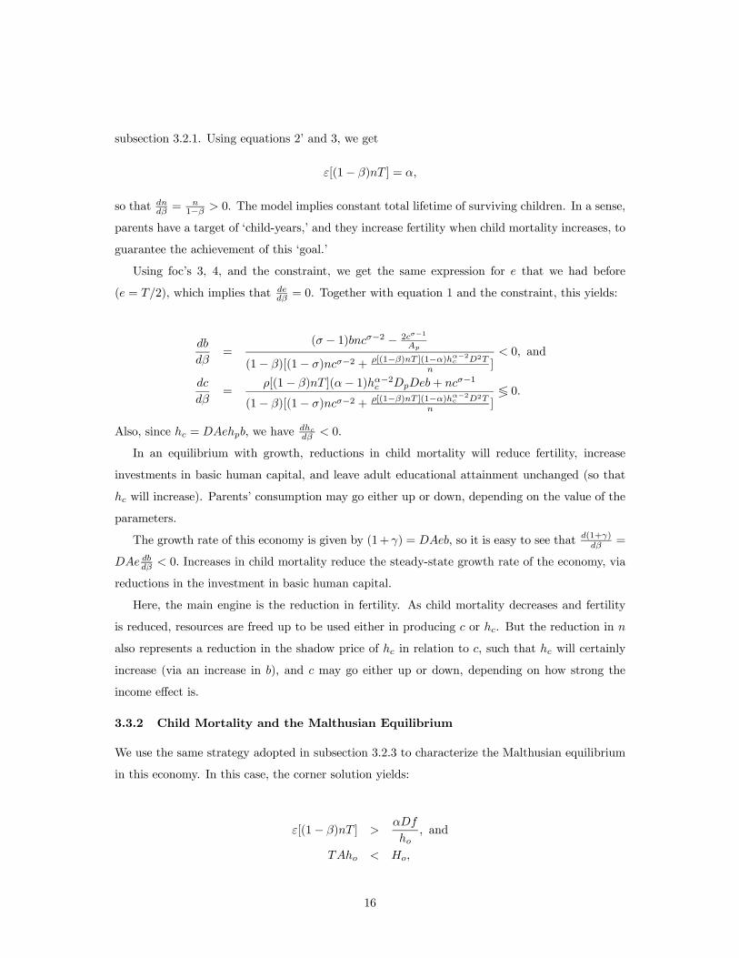
subsection 3.2.1. Using equations 2’ and 3, we get
ε[(1− β)nT ] = α,
so that dndβ =n1−β > 0. The model implies constant total lifetime of surviving children. In a sense,
parents have a target of ‘child-years,’ and they increase fertility when child mortality increases, to
guarantee the achievement of this ‘goal.’
Using foc’s 3, 4, and the constraint, we get the same expression for e that we had before
(e = T/2), which implies that dedβ = 0. Together with equation 1 and the constraint, this yields:
db
dβ=
(σ − 1)bncσ−2 − 2cσ−1Ap
(1− β)[(1− σ)ncσ−2 + ρ[(1−β)nT ](1−α)hα−2c D2Tn ]
< 0, and
dc
dβ=
ρ[(1− β)nT ](α− 1)hα−2c DpDeb+ ncσ−1
(1− β)[(1− σ)ncσ−2 + ρ[(1−β)nT ](1−α)hα−2c D2Tn ]
≶ 0.
Also, since hc = DAehpb, we have dhcdβ < 0.
In an equilibrium with growth, reductions in child mortality will reduce fertility, increase
investments in basic human capital, and leave adult educational attainment unchanged (so that
hc will increase). Parents’ consumption may go either up or down, depending on the value of the
parameters.
The growth rate of this economy is given by (1+ γ) = DAeb, so it is easy to see that d(1+γ)dβ =
DAe dbdβ < 0. Increases in child mortality reduce the steady-state growth rate of the economy, via
reductions in the investment in basic human capital.
Here, the main engine is the reduction in fertility. As child mortality decreases and fertility
is reduced, resources are freed up to be used either in producing c or hc. But the reduction in n
also represents a reduction in the shadow price of hc in relation to c, such that hc will certainly
increase (via an increase in b), and c may go either up or down, depending on how strong the
income effect is.
3.3.2 Child Mortality and the Malthusian Equilibrium
We use the same strategy adopted in subsection 3.2.3 to characterize the Malthusian equilibrium
in this economy. In this case, the corner solution yields:
ε[(1− β)nT ] >αDf
ho, and
TAho < Ho,
16

which are analogous to the inequalities obtained before. The behavior of n and c in this equilibrium
can be analyzed using the foc’s and the constraint:
dn
dβ=
Thα
o
α {ρ0[(1− β)nT ] + (1− β)nTρ00[(1− β)nT ]}(1− β)2T 2ρ00(nT )h
αo
α + f2
T (σ − 1)cσ−2≶ 0, and
dc
dβ=−f h
α
o
α {ρ0[(1− β)nT ] + (1− β)nTρ00[(1− β)nT ]}(1− β)2T 2ρ00(nT )h
αo
α + f2
T (σ − 1)cσ−2≷ 0.
Note that these two expressions will never have the same sign: if one is positive, the other
must be negative. This had to be the case, since changes in β do not change the individual
constraint, so that if one wants to increase the ‘consumption’ of some ‘good’, one has to decrease
the ‘consumption’ of the other.
Anyhow, no matter what happens to n and c, reductions in child mortality will increase
the total number of surviving ‘child-years’ ((1 − β)nT ), and will push the economy away from
the Malthusian steady-state, into a steady-state with growth and positive investments in human
capital. The difference here is that, at first, when β changes, nothing happens to the incentives
to invest in adult human capital (second inequality), and only investments in basic human capital
are undertaken. Only after basic human capital (hc) is accumulated from one generation to the
next, the incentives to invest in adult education increase. And if child mortality reduction is large
enough, the economy enters a sustained growth path. These claims are proved in Appendix A.4.15
3.3.3 Costs of Children Depending on Number of Surviving Children
In our analysis of the effects of child mortality, we assumed that costs of children depend on
the number of born children. Our results would change considerably if costs of having children
depended on the number of surviving children. Which one of the two specifications is the most
accurate description of reality is an empirical matter. It probably depends crucially on which phase
of childhood concentrates most of the reductions in mortality. We come back to this discussion
in the empirical section. For now, we briefly explore the theoretical consequences of changing the
assumptions related to the costs of having children.
Once we assume that costs of children depend on the number of surviving children, the time
and goods constraints have to be substituted by the following:
15 There are some appealing variations of the basic model that do not introduce any major change in terms ofthe qualitative results. For example, if instead of facing increases in their longevity together with their children’s,parents face only increases in children’s longevity, we arrive at similar conclusions. Generally, increases in futuregenerations’ adult longevity have the same short run effects of reductions in child mortality, and the same long runeffects of overall increases in adult longevity. Also, if utility from children depends only on shared lifetime (betweenparents and children), there is no change at all in the qualitative results.
17
lHp > Tc+ f(1− β)n, and
T > l + b(1− β)n+ e,
and the rest of the problem remains unchanged.
The only role of a change in child mortality in this set up will be to change the fertility rate,
in such a way as to maintain exactly the same number of surviving children (n = (1 − β)n, the
net fertility rate), given constant values of the other parameters. Since child mortality affects the
costs and benefits of having children in the same way, parents have a target number of surviving
children that is kept no matter what is the child mortality rate. Reductions in child mortality
reduce the fertility rate, and leave the other variables unchanged. There is no effect on growth or
human capital accumulation, and reductions in child mortality do not tend to move the economy
out of a Malthusian regime.
4 Empirical Evidence
4.1 The Nature and Timing of Mortality Changes
The theory presented here predicts that a Malthusian economy experiencing increases in life
expectancy ((1−β)T ) would go through an initial phase with consumption and fertility changing
in different ways — depending on the particular value of the parameters — and with population
increasing rapidly.16 This population increase would be driven mainly by the gains in life
expectancy itself. If these gains were significant enough, individuals would start investing in
human capital and the economy would move to a new equilibrium with the possibility of long run
growth. From this point on, educational attainment would rise with gains in adult longevity, and
fertility would be reduced by either reductions in child mortality or increases in adult longevity.
Further increases in life expectancy in this new equilibrium would be associated with further
reductions in fertility, and increases in human capital accumulation and growth.
For this theory to be empirically relevant, it must be the case that longevity gains actually
preceded fertility reductions in the real experiences of demographic transition. Besides, it must
16 At any point in time, population is an intricate function of the cumulative effect of past fertility and childmortality rates on initial population levels, and also a function of adult longevity. If we normalize our model insuch a way that parents have children in the end of their first period of life (τ = 1), and we call Ps the populationat period s, we have that:
Ps =
s−1Xj=s−T
jYi=s−T
(1− βi)ni
Ps−T−1 = s−1Xj=s−T
jYi=0
(1− βi)ni
P0,where s > T , and P0 is the initial population.
18

also be the case that mortality reductions were somewhat exogenous to economic development.
Figure 1 presents the most obvious evidence that a large share of the changes in life expectancy
was not determined by development. If we add to this the evidence from Preston (1975), we realize
that a large part of the mortality changes throughout the twentieth century was unrelated to
changes in income.17 Similar evidence is available regarding the relation between life expectancy
and nutrition. Preston (1980, p.305) presents data on life expectancy at birth and nutrition for
a cross-section of countries in 1940 and 1970. He shows that life expectancy gains took place at
every nutrition level. For the lowest nutrition level (less than 2,100 calories daily), there was an
increase of 10 years in life expectancy at birth. He also relates life expectancy changes to both
income and calories consumption, and concludes that approximately 50% of the changes in life
expectancy were due to what he calls ‘structural factors,’ unrelated to economic development.
Further evidence is related to the nature of the diseases responsible for mortality reductions in
the different countries. Preston (1980, p.300-313) argues that the role of economic development in
reducing mortality probably operated mostly through influenza/pneumonia/bronchitis, for which
there was no effective deployment of preventive measures, and diarrheal diseases, for which the
improvements came mainly through improvement in water supply and sewerage. Apart from
these diseases, preventive measures were probably the most effective ones. Simple changes in
public practices and personal health behavior, brought about by knowledge previously inexistent,
allowed for significant reductions in mortality at very low costs (Preston, 1996, p.532-4).18 This
view generates numbers similar to the ones obtained in the income—nutrition—mortality analysis,
with a little more than 50% of the life expectancy gains being unrelated to economic development
per se.19
Regarding the timing of events during the transition, the usual description depicts mortality
reductions starting the process, implying a period of intense population growth, which progres-
sively diminishes as fertility starts to decline. Also, initial economic conditions are seen as being
17 We do not claim that improvements in living conditions do not affect life prospects. This relation is, indeed,an important part of the mechanism of checks and balances behind the Malthusian model. Our claim is just thatchanges in life expectancy at birth from 40 to more than 70 years, like the ones experienced during the demographictransition, are largely not due to material improvements.
18 Most dramatically, the acceptance of the germ theory — developed on the turn of the nineteenth to the twentiethcentury — allowed for inexpensive gains in life expectancy via simple preventive measures (Vacher, 1979; Ram andSchultz, 1979; Preston, 1980 and 1996; Ruzicka and Hansluwka, 1982). Also, throughout the twentieth century,health programs became increasingly dissociate of the countries’ economic conditions, and more dependent on theconcerns of the developed world. Even though the monetary value of the help was relatively small, the largercontributions came in the form of development of low cost health measures, training of personnel, initiation ofprograms, and more effective and specific interventions (see Preston, 1980, p.313-5; and Ruzicka and Hansluwka,1982). This, to some extent, helped to dissociate gains in life expectancy from improvements in economic conditions.
19 The evidence presented in Becker, Philipson, and Soares (2002), regarding the diseases responsible for thecross-country convergence in life expectancy, also supports this view.
19

extremely diverse in the different cases (see Heer and Smith, 1968; Cassen, 1978; Kirk, 1996;
Mason, 1997; and Macunovich, 2000). In this direction, if we look at the more recent experience
of developing countries, we see cases of modest longevity gains without fertility reductions, but we
do not see cases of fertility reductions without longevity gains (see Soares, 2002a). The features
of the data are consistent with the theory. Initial life expectancy gains, while the economy is
still in the Malthusian equilibrium, may have distinct effects on fertility. But, inevitably, further
mortality reductions end up moving the economy out of this equilibrium. Once this threshold is
reached, fertility decreases with gains in life expectancy.
Additionally, the data supports the idea that there may be a cut off level of life expectancy that
determines the escape from the Malthusian equilibrium. Strictly, this cut off level could be country
specific, depending on cultural and natural aspects. But the evidence discussed above is consistent
with a common threshold around 50 years of life expectancy at birth. If this is the case, reaching
this level of life expectancy would mark the transition of a country from a Malthusian regime to
an equilibrium with investments in human capital and the possibility of sustained growth.
In Figures 6 and 7 we explore this point, by analyzing the behavior of fertility and educational
attainment before and after the year when life expectancy at birth reaches 50. Obviously, we do not
imply that this specific number is the precise point at which all the different countries start their
demographic transition. Rather, we think of it as a reasonable approximation to the moment of
change in the demographic regime. Every country that reaches this level of life expectancy within
the interval 1960-95, and for which data is available, is included in the Figures. Countries are
aligned in time according to the year when the threshold was reached, such that the year T is the
‘year when life expectancy at birth reached 50.’ Other years are measured as deviations from this
reference point.
Figure 6 shows the behavior of fertility before and after year T , measured as the deviation
of fertility from its initial transitional level (year T ). The pattern arises clearly. While fertility
behaves very erratically before the year when life expectancy reaches 50, it shows a consistent
downward trend for all countries after this cut off is reached. Figure 7 does the same exercise for
average schooling in the population aged 15 and above. The result shows an analogous pattern:
while educational attainment does not have any clear trend before life expectancy at birth reaches
50, it shows a consistent upward trend for all countries after this cut off point is reached.
The overall historical evidence is consistent with the predictions of the model regarding the
behavior of the economy before and after the triggering of the demographic transition.20 Besides,
20 The behavior of population in the second half of the twentieth century is also consistent with the theory.Heuveline (1999) uses counter factual projections of the behavior of mortality and fertility between 1950 and 2000to disentangle the effect of these two variables on the world population. He extends the methodology applied
20

the data suggest that the transition usually starts at some moment around the time when life
expectancy at birth reaches 50 years. This point will be important in our investigation of the
recent behavior of fertility, educational attainment, and growth in “post-demographic transition”
countries.
4.2 The Behavior of the Economy after the Demographic Transition —Evidence from a Panel of Countries
4.2.1 Estimation Strategy
In this section, we analyze the behavior of fertility, educational attainment, and growth in a panel
of countries, between 1960 and 1995. Our goal is to test whether the relation between these
variables and child mortality and adult longevity agrees with the predictions of the model. In the
model, the behavior of the economy suffers a significant change as we move from the Malthusian
equilibrium to the equilibrium with positive investments in human capital. For this reason, it
does not make sense to compare pre to post-transition economies, since they respond differently
to changes in the exogenous variables. Therefore, we look at economies that had already started
the demographic transition in 1960 and should behave according to the properties of the model
in the equilibrium with growth.
We concentrate on the endogenous variables for which we have observable statistics: fertility,
educational attainment, and growth. The data are averages for five year periods between 1960 and
1995. Variables corresponding to child mortality, adult longevity, fertility, and growth are taken
from the World Bank’sWorld Development Indicators — 1999. These are, initially: child mortality
rate before 1 year (mort), life expectancy conditional on survival to 1 year (adult1), total fertility
rate (fert), and growth rate of the real GNP per capita (growth). Educational attainment is
measured by the average schooling in the population aged 15 and above (schl), from the Barro
and Lee data set (see Barro and Lee, 1993). Other variables are incorporated along the way, to
check the robustness of the initial results. The sample is restricted to countries for which data is
available for all the variables and years. This leaves 70 countries and 8 points in time, which gives
a total of 560 observations. Summary statistics for the relevant variables are presented in Table
4. Appendix B describes the data in more detail, and enumerates the countries included in the
by White and Preston (1996), by dividing the world population into regions, and projecting four counter factualscenarios for each of them separately. The projections are obtained by applying age and sex specific survival ratesto the populations of the different regions, and applying age specific fertility rates to the female population by age.His analysis shows that mortality reductions of the second half of the twentieth century contributed to increasethe world population by, at least, 33%, while fertility changes reduced it by 26%. Interestingly, had the fertilityand mortality levels remained at their 1950 values, the world population today would be virtually the same as itactually is. Contrary to the common belief in the economics profession, the population explosion of the twentiethcentury was caused almost entirely by gains in life expectancy, with fertility changes working towards slowing downthe process.
21
sample.
The first order conditions for the individual problem give implicitly a set of reduced form equa-
tions that express fertility, education, and growth as functions of child mortality, adult longevity,
and the other exogenous variables:
fert = f(mort, adult1,X),
schl = g(mort, adult1,X), and
growth = q(mort, adult1,X),
where X denotes all other exogenous variables apart from child mortality and adult longevity.
Our strategy is to take the model seriously and estimate these reduced form equations. Apart
from the life expectancy variables, the only exogenous factors in our model are related to tastes
(parameters of the utility function) and technology (parameters of the production functions). To
account for shifts in these exogenous variables across countries, we use country fixed effects, so
that any systematic difference due to culture, religion, and technology is washed away. Also, to
account for technological development or absorption through time, we include time dummies.
The issue of exogeneity of the life expectancy gains becomes extremely important here. To
control for the changes in life expectancy that are simply a consequence of economic development,
we include the natural logarithm of the real GNP per capita (ln gnp) in the reduced forms above.
This will isolate the changes due to life expectancy, from those directly attributable to development
and to behavioral changes induced by increases in income.
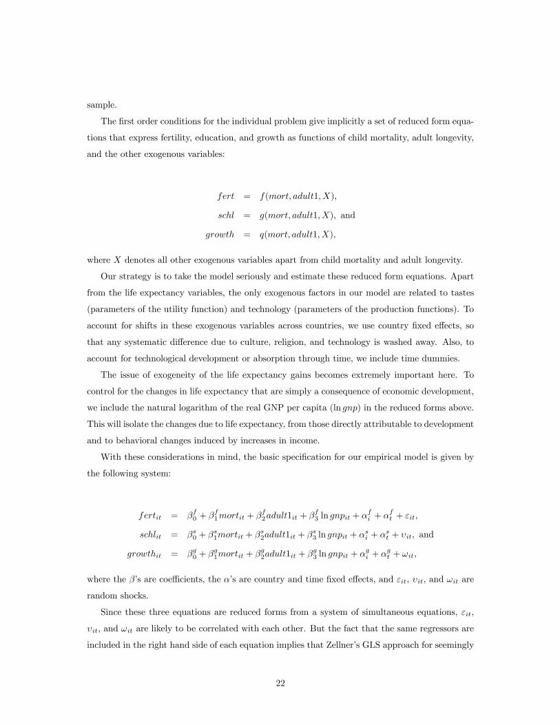
With these considerations in mind, the basic specification for our empirical model is given by
the following system:
fertit = βf0 + βf1mortit + βf2adult1it + βf3 ln gnpit + αfi + αft + εit,
schlit = βs0 + βs1mortit + βs2adult1it + βs3 ln gnpit + αsi + αst + υit, and
growthit = βg0 + βg1mortit + βg2adult1it + βg3 ln gnpit + αgi + αgt + ωit,
where the β’s are coefficients, the α’s are country and time fixed effects, and εit, υit, and ωit are
random shocks.
Since these three equations are reduced forms from a system of simultaneous equations, εit,
υit, and ωit are likely to be correlated with each other. But the fact that the same regressors are
included in the right hand side of each equation implies that Zellner’s GLS approach for seemingly
22

unrelated regressions and simple OLS estimation generate the same results. Therefore, this issue
is of no concern.21
Finally, our goal is to test the model predictions in relation to economies in the steady-state
with growth, where there are positive investments in human capital. Not all the countries included
in the sample had already left the Malthusian regime in 1960, and this may bias the estimates.
For this reason, we estimate the model both for the whole sample and for a sample of selected
countries, that supposedly had already started the demographic transition in 1960 (post-transition
countries). Although it is always difficult to define a precise criterion that identifies a country
as being or not in the Malthusian regime, this is a problem we cannot avoid. We assume that
countries with life expectancy at birth above 50 years in 1960 had already escaped the Malthusian
equilibrium, as the evidence from section 4.1 suggests. The list of countries included in the selected
sample is contained in Appendix B, and it shows that the criterion chosen seems to be a reasonable
one.
4.2.2 Analysis of the Results
For illustrational purposes, Table 2 presents regression results for the whole sample. The first
column presents regressions of the three endogenous variables on only child mortality and adult
life expectancy, the second column includes per capita income in the right hand side, and the last
column includes country and time fixed effects.
Table 3 presents the results for the selected sample (post-transition countries), using the full
specification discussed above. The model performs well empirically. All coefficients on adult
longevity are significant and have the expected sign. In relation to child mortality, the coefficient
of the fertility equation is significant and have the expected effect. The coefficients of the growth
and schooling equations are not significant.
The evidence that adult longevity reduces fertility and increases educational attainment and
growth, while child mortality only has a significant effect on fertility, supports the version of
the model discussed in subsection 3.3.3. There, we argued that when costs of having children
depend on the number of surviving children, changes in child mortality will only affect fertility,
and leave educational attainment and growth unchanged. This could be a consequence of the
fact that we are dealing here only with child mortality before 1 year, when probably not many
investments in children have been undertaken. But, since reductions in child mortality have been
largely concentrated on very early ages (mainly below 1 year), and mortality rates between 5 years
and young adulthood are extremely low, we do believe that such a version of the model may be,
21 All the results discussed here remain the same once we allow for panel specific AR1 auto-correlation in theresiduals.
23

empirically, the most relevant one. We come back to this point later on.
The comparison of the results from the same specification in the whole sample (Table 2, column
3) with the ones in the selected sample (Table 3) also agree with the theory. Regarding adult
longevity, the coefficient of the schooling equation in the whole sample is not significant, and the
coefficients of the fertility and growth equations are considerably smaller than the ones obtained
in the selected sample. Also the child mortality coefficient of the fertility equation is smaller in
the whole sample when compared to the selected sample. Since the predictions being tested apply
only to economies that have already started the demographic transition, we should expect the
whole sample to deliver results weaker than the ones found in the selected sample.
Nevertheless, the results may still be due to spurious correlation or to omitted variable bias.
The theory developed here implies that adult longevity gains should increase investments in edu-
cation, reduce fertility, and spur economic growth only if these gains took place during productive
lifetime. Longevity gains concentrated at very old ages, when individuals do not or cannot work
anymore, should not have the same effects, since they do not affect the horizon over which invest-
ments in human capital can be used. Given that significant reductions in mortality at old ages
have been observed in the more developed countries, this issue should be of concern. If this is
what is driving our empirical results, the evidence does not support the causal links predicted by
the model. Also, as mentioned before, the evidence regarding child mortality may be driven by
the fact that we are considering only child mortality before 1 year, and significant mortality rates
still occur until the age of 5.
To check whether our results reflect the causal relations stressed by the model, we repeat the
exercise from Table 3 breaking down adult longevity into productive life expectancy and old age
life expectancy, and using both child mortality before 1 year and child mortality before 5 years.
This is done using data on adult mortality rates between 15 and 60 years, together with child
mortality and life expectancy at birth (see Appendix B).
The first two variables constructed are expected years of life between 15 and 60 years (adexp),
and life expectancy conditional on survival to 60 years (oldexp). We estimate a regression similar
to the one presented in Table 3, breaking down adult longevity into these two variables. The
inclusion of the new variable reduces the sample considerably, so much so that we are left only
with observations for the years 1960, 1970, 1980, 1990, and 1995, for 46 countries. The results are
presented in the first three columns of Table 4. As should be expected if the results were driven
by gains in longevity during productive life, old age life expectancy (oldexp) is not significant
in any of the equations. The effect of child mortality (mort) on fertility is extremely close to
the one observed in Table 3. All the results on productive adult life expectancy (adexp) are still
24

significant, and the effects on fertility and educational attainment are considerably larger than the
ones obtained before.
To check whether our child mortality variable affected the results, we repeat the exercise
described in the previous paragraph using child mortality rate before 5 years. This redefines the
child mortality rate and old age life expectancy as, respectively, mort5 and oldexp5. The choice of
this variable reduces the sample even further, and we are left with observations for the years 1960,
1970, 1980, 1990, and 1995, for only 41 countries. Nevertheless, the results — presented in columns
4 to 6 of Table 4 — are still extremely similar to the ones from Table 3. The only noticeable
difference is the fact that productive life expectancy (adexp) is only borderline significant for the
fertility regression.22
This evidence is supportive of the causal links established by the theory. It shows that the
effects captured in Table 3 come from longevity gains during productive years, and not from old
age mortality reductions. This is the precise mechanism on which the logic of the model relies.
Also, the results show that the choice of the child mortality variable did not introduce any bias.
Finally, we try a last robustness check. We instrument for adult life expectancy using the
percentage of the population with access to safe water. It is very difficult to find an instrument
for adult longevity that performs well in the first stage once we are already controlling for income.
We tried several other variables (immunization rates, physicians per capita, pollution measures,
percentage of the population with access to sanitation, and percentage of population and area
affected by malaria) unsuccessfully. The variable chosen — percentage of population with access
to safe water — performs reasonably well in the first stage: it is significant and adds 1.5% to
the other variable’s explanatory power in relation to adult longevity. Nevertheless, the second
stage results are poor. The three last columns of Table 4 present the results of the IV estimation.
Adult life expectancy has a negative and significant effect on fertility and a positive and borderline
significant effect on schooling. But the magnitude of these coefficients is implausibly large, and
the coefficient on growth is negative, though not significant. We do not take these results too
seriously, and present them mainly as an evidence of the difficulty of using instrumental variables
in this context.
Going back to Table 3, the quantitative implications of the estimated coefficients are also of
interest. The model predicts that a 10 year gain in adult longevity implies a reduction of 1.7
points in total fertility rate, an increase of 0.7 year in average schooling in the population aged
15 and above, and a growth rate higher by 4.6%. A reduction of 100 per one thousand in child
22 It is difficult to tell whether this is caused by the change in the variable or by the reduction in the size of thesample.
25
mortality implies a reduction of 2 points in the total fertility rate.
These results are in line with a vast array of evidence from studies that try to estimate the
economic impacts of life expectancy gains. Most notoriously, these include the positive effect of
life expectancy on growth in the traditional empirical growth literature, summarized and discussed
in Barro and Sala-i-Martin (1995). Other examples are the case study for India of the effects of
life expectancy gains on schooling and productivity (Ram and Schultz, 1979), and the simulation
exercises performed by Bils and Klenow (2000), analyzing the role of life expectancy in explaining
cross-country differences in schooling, productivity, and fertility.
Elsewhere (Soares, 2002b), we show that the relation between adult longevity, fertility, and
educational attainment portrayed here is also present in individual level data. We use family and
state specific mortality indicators and data from the Brazilian Demographic and Health Survey to
show that adult longevity is positively related to educational attainment and negatively related
to fertility, after child mortality and a large set of demographic variables are accounted for.
5 Concluding Remarks
This paper explores the link between life expectancy, educational attainment, and fertility choice.
We show that, under reasonable conditions, mortality reductions can explain the movement of
economies from a Malthusian equilibrium, with no investments in human capital, to a steady-state
with growth. Further reductions in mortality in this steady-state with growth reduce fertility,
increase educational attainment, and, thus, increase the growth rate of the economy. These
features of the model help explain the demographic transition throughout the world and the
recent behavior of fertility in post-demographic transition countries.
Two aspects of the model drive these effects, and distinguish our theoretical work from the
previous literature. The utility that parents derive from each child is allowed to depend on the
number of children and, additionally, on the lifetime that each child will enjoy as an adult. The
way number of children and lifetime of each child interact in the parent’s utility function is an
important force behind the mechanics of the model.
Also, human capital investments are broken down in two pieces: basic investments, that take
place during childhood and are done by parents; and adult investments, that take place during
adulthood and are done by the individuals themselves. We interpret educational attainment as
the time that adult individuals spend on their own education. Besides being more realistic, this
approach allows the model to distinguish between the effects of adult longevity and child mortality
on investments in education and growth.
Through these two channels, gains in adult longevity can move an economy out of a steady
26
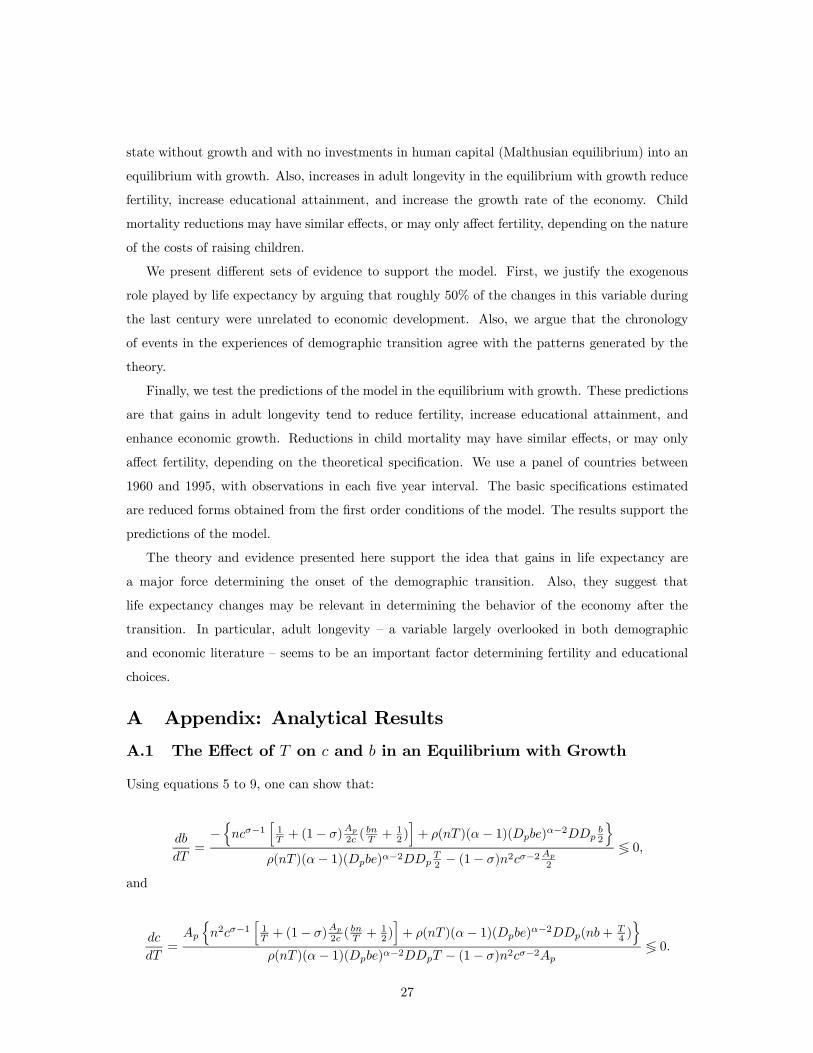
state without growth and with no investments in human capital (Malthusian equilibrium) into an
equilibrium with growth. Also, increases in adult longevity in the equilibrium with growth reduce
fertility, increase educational attainment, and increase the growth rate of the economy. Child
mortality reductions may have similar effects, or may only affect fertility, depending on the nature
of the costs of raising children.
We present different sets of evidence to support the model. First, we justify the exogenous
role played by life expectancy by arguing that roughly 50% of the changes in this variable during
the last century were unrelated to economic development. Also, we argue that the chronology
of events in the experiences of demographic transition agree with the patterns generated by the
theory.
Finally, we test the predictions of the model in the equilibrium with growth. These predictions
are that gains in adult longevity tend to reduce fertility, increase educational attainment, and
enhance economic growth. Reductions in child mortality may have similar effects, or may only
affect fertility, depending on the theoretical specification. We use a panel of countries between
1960 and 1995, with observations in each five year interval. The basic specifications estimated
are reduced forms obtained from the first order conditions of the model. The results support the
predictions of the model.
The theory and evidence presented here support the idea that gains in life expectancy are
a major force determining the onset of the demographic transition. Also, they suggest that
life expectancy changes may be relevant in determining the behavior of the economy after the
transition. In particular, adult longevity — a variable largely overlooked in both demographic
and economic literature — seems to be an important factor determining fertility and educational
choices.
A Appendix: Analytical Results
A.1 The Effect of T on c and b in an Equilibrium with Growth
Using equations 5 to 9, one can show that:
db
dT=−nncσ−1
h1T + (1− σ)
Ap2c (
bnT +
12)i+ ρ(nT )(α− 1)(Dpbe)α−2DDp b2
oρ(nT )(α− 1)(Dpbe)α−2DDp T2 − (1− σ)n2cσ−2Ap2
≶ 0,
and
dc
dT=Ap
nn2cσ−1
h1T + (1− σ)
Ap2c (
bnT +
12)i+ ρ(nT )(α− 1)(Dpbe)α−2DDp(nb+ T
4 )o
ρ(nT )(α− 1)(Dpbe)α−2DDpT − (1− σ)n2cσ−2Ap≶ 0.
27

But note that, if dcdT < 0, we have
n2cσ−1·1
T+ (1− σ)
Ap2c(bn
T+1
2)
¸+ ρ(nT )(α− 1)(Dpbe)α−2DDp(nb+ T
4) > 0.
Since nb+ T4 >
nb2 , this implies that
n2cσ−1·1
T+ (1− σ)
Ap2c(bn
T+1
2)
¸+ ρ(nT )(α− 1)(Dpbe)α−2DDpnb
2> 0,
which in turn implies that dbdT > 0.
Also, if dbdT < 0, we have
n2cσ−1·1
T+ (1− σ)
Ap2c(bn
T+1
2)
¸+ ρ(nT )(α− 1)(Dpbe)α−2DDpnb
2< 0.
Again, since nb+ T4 >
nb2 , this implies that
n2cσ−1·1
T+ (1− σ)
Ap2c(bn
T+1
2)
¸+ ρ(nT )(α− 1)(Dpbe)α−2DDp(nb+ T
4) < 0,
which in turn implies that dcdT > 0.
In words, dcdT ordbdT may be negative, but both cannot be negative at the same time. If one of
them is negative, the other must be positive.
A.2 The Possibility of a Steady-State
The possibility of a steady-state in this economy rests on the values of the parameters α and σ.
Technological factors summarized by the goods constraint imply that, in any steady-state, c and
hp must necessarily grow at the same constant rate from one generation to the next. But the
individual maximization problem tells us, through equation 8, that c and hp growing at the same
rate will not be consistent with the optimal choices of the different generations, unless α = σ.
Therefore, for a steady-state to exist in this economy, it must be the case that α = σ, so that
individuals from different generations will make optimal choices such that c and hp will grow at
the same constant rate, and b, n, e, and l will be constant.
This can be formally seen once we realize that, in terms of the individual’s problem, for a
steady-state to exist it must be the case that agents will not change their decisions regarding n,
b, l, and e as hp increases. This means that the different generations, who differ only in terms of
their endowed hp and see it as a given parameter, will translate the higher levels of basic human
capital in increased consumption, leaving b, n, e, and l unchanged.
From the results obtained before, we already know that dndhp
= dedhp
= 0. We can use equations
7 and 8 to show how b and c respond to changes in hp. This gives the following expressions:
28

db
dhp=
(σ − 1)behp[(σ − α)bn+ (α− 1)e] −
b
hp≷ 0, and
dc
dhp=
Ae2(1− α)(bn− e)T [(σ − α)bn+ (α− 1)e] > 0,
where the sign of dcdhp
comes from the fact that σ < 1.
As mentioned before, a steady-state requires a constant b with an increasing hp. This will only
happen here if σ = α, in which case we have dbdhp
= 0 and dcdhp
= AT e(e−bn). It is immediate to see
that, in this case, c and hp will grow at the same constant rate, given by (1 + γ) = hchp= DAbe.
If σ 6= α, there is no steady-state, and b will increase or decrease over time (with the increase
in hp) until a corner solution is reached. Rewrite dbdhp
in the following way:
db
dhp=b
hp
(σ − α)(e− bn)[(σ − α)bn+ (α− 1)e] .
So, if α > σ, we have dbdhp
> 0; and if α < σ, we have dbdhp
< 0, since σ < 1.
The intuition for this result is clear. If α > σ, the sub-utility function related to hc is less
concave than the one related to c, such that when hp grows from one generation to the next,
younger generations tend to increase hc more than proportionately to c, and this is achieved
through increases in b. The same sort of argument works for the case where α < σ, implying that
hc is increased less than proportionately to c, and that this is achieved through reductions in b.
When α = σ, every generation is just happy to increase c and hp in the same proportion in relation
to the previous generation, in which case b remains unchanged and we have a steady-state.
A.3 The Effect of T on the Malthusian Equilibrium
A.3.1 The Malthusian Equilibrium
We call the corner solution in human capital investments a Malthusian equilibrium because, in a
situation like this, changes in productivity — brought about, for example, by exogenous changes
on Ho — will be positively correlated with changes in both consumption and fertility. This can
be seen by analyzing the effect of an exogenous change in Ho. Using the first two foc’s and the
constraint, we arrive at:
dn
dHo=
f(σ − 1)cσ−2T 2ρ00(nT )h
αo
α + f2
T (σ − 1)cσ−2> 0, and
dc
dHo=
Tρ00(nT )hα
o
α
T 3ρ00(nT )hαo
α + f2(σ − 1)cσ−2> 0.
29

Fertility and consumption respond positively to exogenous increases in productivity. If we
want this set up to display all the features of a so called Malthusian regime, including its checks
and balances mechanisms and the zero long run growth in consumption, we can substitute Ho by
some function F (Ho, P ). In this case, P denotes the aggregate population level, and FHo(., .) > 0.
Decreasing marginal product in the agriculture sector due to limited availability of land would
be captured by FP (., .) < 0, such that, for a given level of Ho, individual productivity decreases
with total population. This externality implies that exogenous increases in Ho generate short run
increases on n and c, that are ‘consumed’ in the long run by the expanded population. With
time, n returns to its long run equilibrium value — given by (1− β)n = 1, such that population is
constant — which also pins down the long run value of consumption. In this equilibrium, there are
no long run improvements on living standards, and population grows only to the extent allowed by
exogenous technical improvements or positive natural shocks (increases on Ho). This additional
feature of the model captures all the properties of what is known as a Malthusian regime, but to
keep things simple we analyze the case where F (Ho, P ) = Ho. As long as the effect of P takes
some time to operate, our results will be quite general.
A.3.2 Changes on T while the Corner Solution Holds
In this case, only n and c will be affected by T . The effect of T on n and c in the Malthusian
equilibrium can be obtained from the first two foc’s and the constraint.
dn
dT=
f2nT2 (σ − 1)cσ−2 − h
α
o
α [nTρ00(nT ) + ρ0(nT )]
T 2ρ00(nT )hαo
α + f2
T (σ − 1)cσ−2≶ 0, and
dc
dT=
fhα
o
α [2nTρ00(nT ) + ρ0(nT )]
T 3ρ00(nT )hαo
α + f2(σ − 1)cσ−2≷ 0.
If dndT < 0, it means that nTρ00(nT )+ρ0(nT ) < 0, which implies that 2nTρ00(nT )+ρ0(nT ) < 0,
which in turn implies that dcdT > 0.
Also, if dcdT < 0, we have 2nTρ00(nT )+ρ0(nT ) > 0, which implies that nTρ00(nT )+ρ0(nT ) > 0,
which in turns implies that dndT > 0.
In other words, dcdT or dn
dT may be negative, but both cannot be negative at the same time.
Either c or n must increase as T increases. Besides, a sufficient condition for both of them to be
positive is that −nTρ00(nT ) < ρ0(nT ) < −2nTρ00(nT ).
A.3.3 The Escape from the Malthusian Steady-State
We want to look at what happens to the two last first order conditions as T increases. We start
by analyzing the steady-state where investment in both forms of human capital is zero, and show
30
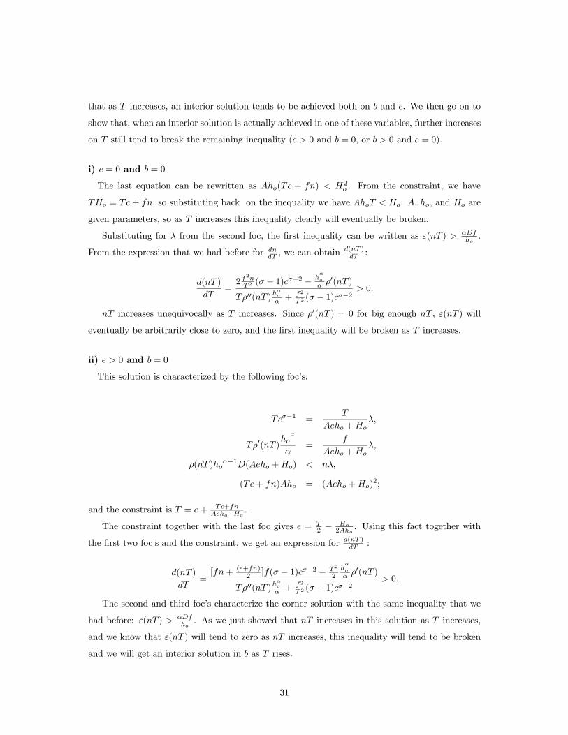
that as T increases, an interior solution tends to be achieved both on b and e. We then go on to
show that, when an interior solution is actually achieved in one of these variables, further increases
on T still tend to break the remaining inequality (e > 0 and b = 0, or b > 0 and e = 0).
i) e = 0 and b = 0
The last equation can be rewritten as Aho(Tc + fn) < H2o . From the constraint, we have
THo = Tc+ fn, so substituting back on the inequality we have AhoT < Ho. A, ho, and Ho are
given parameters, so as T increases this inequality clearly will eventually be broken.
Substituting for λ from the second foc, the first inequality can be written as ε(nT ) > αDfho.
From the expression that we had before for dndT , we can obtain
d(nT )dT :
d(nT )
dT=2f
2nT 2 (σ − 1)cσ−2 − h
α
o
α ρ0(nT )
Tρ00(nT )hαo
α + f2
T 2 (σ − 1)cσ−2> 0.
nT increases unequivocally as T increases. Since ρ0(nT ) = 0 for big enough nT , ε(nT ) will
eventually be arbitrarily close to zero, and the first inequality will be broken as T increases.
ii) e > 0 and b = 0
This solution is characterized by the following foc’s:
Tcσ−1 =T
Aeho +Hoλ,
Tρ0(nT )ho
α
α=
f
Aeho +Hoλ,
ρ(nT )hoα−1D(Aeho +Ho) < nλ,
(Tc+ fn)Aho = (Aeho +Ho)2;
and the constraint is T = e+ Tc+fnAeho+Ho
.
The constraint together with the last foc gives e = T2 − Ho
2Aho. Using this fact together with
the first two foc’s and the constraint, we get an expression for d(nT )dT :
d(nT )
dT=[fn+ (e+fn)
2 ]f(σ − 1)cσ−2 − T2
2hα
o
α ρ0(nT )
Tρ00(nT )hαo
α + f2
T 2 (σ − 1)cσ−2> 0.
The second and third foc’s characterize the corner solution with the same inequality that we
had before: ε(nT ) > αDfho. As we just showed that nT increases in this solution as T increases,
and we know that ε(nT ) will tend to zero as nT increases, this inequality will tend to be broken
and we will get an interior solution in b as T rises.
31
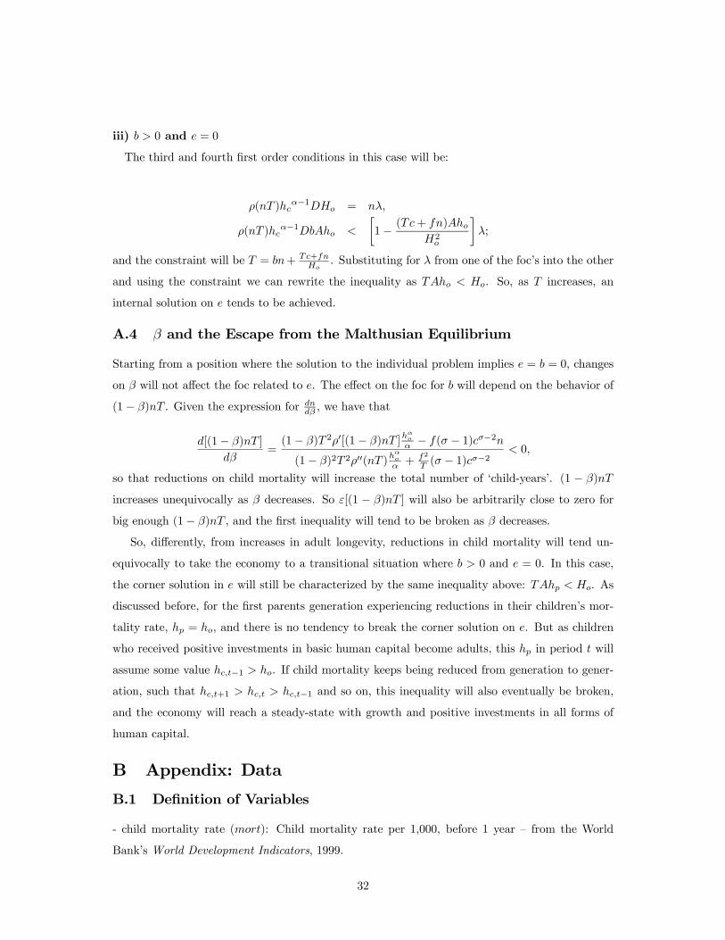
iii) b > 0 and e = 0
The third and fourth first order conditions in this case will be:
ρ(nT )hcα−1DHo = nλ,
ρ(nT )hcα−1DbAho <
·1− (Tc+ fn)Aho
H2o
¸λ;
and the constraint will be T = bn+ Tc+fnHo
. Substituting for λ from one of the foc’s into the other
and using the constraint we can rewrite the inequality as TAho < Ho. So, as T increases, an
internal solution on e tends to be achieved.
A.4 β and the Escape from the Malthusian Equilibrium
Starting from a position where the solution to the individual problem implies e = b = 0, changes
on β will not affect the foc related to e. The effect on the foc for b will depend on the behavior of
(1− β)nT . Given the expression for dndβ , we have that
d[(1− β)nT ]
dβ=(1− β)T 2ρ0[(1− β)nT ]
hαoα − f(σ − 1)cσ−2n
(1− β)2T 2ρ00(nT )hαo
α + f2
T (σ − 1)cσ−2< 0,
so that reductions on child mortality will increase the total number of ‘child-years’. (1 − β)nT
increases unequivocally as β decreases. So ε[(1 − β)nT ] will also be arbitrarily close to zero for
big enough (1− β)nT , and the first inequality will tend to be broken as β decreases.
So, differently, from increases in adult longevity, reductions in child mortality will tend un-
equivocally to take the economy to a transitional situation where b > 0 and e = 0. In this case,
the corner solution in e will still be characterized by the same inequality above: TAhp < Ho. As
discussed before, for the first parents generation experiencing reductions in their children’s mor-
tality rate, hp = ho, and there is no tendency to break the corner solution on e. But as children
who received positive investments in basic human capital become adults, this hp in period t will
assume some value hc,t−1 > ho. If child mortality keeps being reduced from generation to gener-
ation, such that hc,t+1 > hc,t > hc,t−1 and so on, this inequality will also eventually be broken,
and the economy will reach a steady-state with growth and positive investments in all forms of
human capital.
B Appendix: Data
B.1 Definition of Variables
- child mortality rate (mort): Child mortality rate per 1,000, before 1 year — from the World
Bank’s World Development Indicators, 1999.
32

- child mortality rate before 5 years (und5): Child mortality rate per 1,000, before 5 years — from
the World Bank’s World Development Indicators, 1999.
- life expectancy at birth (life): Life expectancy at birth — from the World Bank’s World Devel-
opment Indicators, 1999.
- adult mortality rate (admort): Mortality rate per 1,000 between the ages 15 and 60 — from the
World Bank’s World Development Indicators, 1999.
- adult longevity (adult1): Life expectancy conditional on survival to 1 year. Calculated from life
and mort according to the expression life = mort1,0001+(1− mort
1,000)adult1. It corresponds to assuming
that these are the only two variables that compose life expectancy at birth. So, the component of
life expectancy not related to child mortality is assigned to life expectancy conditional on survival
to 1 year. It is assumed that the death of a child occurs at age 1. Results are not sensible to this
normalization.
- young adult longevity (adexp): Expected years of life between 15 and 60 years. Calculated from
admort according to adexp = (1− admort1,000 )45.
- old adult longevity using child mortality rate before 1 year (oldexp): Life expectancy conditional
on survival to 60 years. Calculated from life, mort, and admort according to life =.mort1,0001+(1−mort1,000)[
admort1,000 45 + (1− admort
1,000 )oldexp]. The logic is the same behind the calculation of adult1. It
is assumed that the death of an adult individual occurs at age 45. Results are not sensible to this
normalization.
- old adult longevity using child mortality rate before 5 years (oldex5): Life expectancy conditional
on survival to 60 years. Calculated analogously to oldexp, according to life =. und51,0005 + (1 −mort1,000)[
admort1,000 45 + (1− admort
1,000 )oldex5].
- fertility (fert): Total fertility rate — from the World Bank’sWorld Development Indicators, 1999.
- educational attainment (schl): Average schooling years in the population aged 15 and over —
from the Barro and Lee (1993) updated data set.
- income growth (growth): Growth rate of the GNP per capita (constant 1995 US$) — from the
World Bank’s World Development Indicators, 1999.
- income (gnp): GNP per capita (constant 1995 US$) — from the World Bank’sWorld Development
Indicators, 1999.
- Population with access to safe water (water): Percentage of population with access to safe water
— from the World Bank’s World Development Indicators, 1999.
33
B.2 Countries Included in the Sample
- Whole sample (70 countries) — Table 2: Algeria, Argentina, Australia, Austria, Bangladesh, Bar-
bados, Belgium, Botswana, Brazil, Cameroon, Canada, Central African Republic, Chile, Costa
Rica, Denmark, Dominican Republic, Ecuador, El Salvador, Fiji, Finland, France, Ghana, Greece,
Guatemala, Guyana, Honduras, Hong Kong, Hungary, Iceland, Indonesia, Ireland, Israel, Italy,
Jamaica, Japan, Kenya, Korea, Rep., Lesotho, Malawi, Malaysia, Mauritius, Mexico, Nepal,
Netherlands, New Zealand, Nicaragua, Niger, Norway, Pakistan, Panama, Papua New Guinea,
Paraguay, Philippines, Portugal, Singapore, South Africa, Spain, Sri Lanka, Sudan, Swaziland,
Sweden, Switzerland, Thailand, Togo, Trinidad and Tobago, Tunisia, United Kingdom, United
States, Uruguay, Zambia.
- Selected Sample — Post-transition (life expectancy in 1960 > 50; 47 countries) — Table 3: Ar-
gentina, Australia, Austria, Barbados, Belgium, Brazil, Canada, Chile, Costa Rica, Denmark,
Dominican Republic, Ecuador, El Salvador, Fiji, Finland, France, Greece, Guyana, Hong Kong,
Hungary, Iceland, Ireland, Israel, Italy, Jamaica, Japan, Korea, Rep., Malaysia, Mauritius, Mex-
ico, Netherlands, New Zealand, Norway, Panama, Paraguay, Philippines, Portugal, Singapore,
Spain, Sri Lanka, Sweden, Switzerland, Thailand, Trinidad and Tobago, United Kingdom, United
States, Uruguay.
ReferencesBarro, Robert, and J.W. Lee (1993). International Measures of Schooling Years and School-ing Quality. American Economic Review Papers and Proceedings, 86(2), 1993, 218-23.
Barro, Robert J. and Xavier Sala-i-Martin (1995). Economic Growth. New York, McGraw-Hill, Inc., 1995.
Becker, Gary S. (1985). Human capital, effort, and the sexual division of labor. Journal ofLabor Economics, 3 (1985): S33-S58.
Becker, Gary S. (2000). “Declining population in a modern economy.” Unpublished Manu-script, University of Chicago, August 2000.
Becker, Gary S. and Kevin M. Murphy (1992). The division of labor, coordination costs,and knowledge. Quarterly Journal of Economics, 107, n4 (November 1992): 1137-60.
Becker, Gary S., Kevin M. Murphy, and Robert Tamura (1990). Human capital, fertility,and economic growth. Journal of Political Economy, v98, n5 (Part 2, October 1990): S12-37.
Becker, Gary S., Tomas Philipson, and Rodrigo R. Soares (2002). “Growth and mortality inless developed nations.” Unpublished Manuscript, University of Chicago, October 2001.
Ben-Porath, Yoram (1967). The production of human capital and the life cycle of earnings.Journal of Political Economy, v75, n4 (Part 1, August 1967): 352-65.
34

Bils, Mark and Peter J. Klenow (2000). “Explaining differences in schooling across countries.”Unpublished Manuscript, University of Chicago, January 2000.
Blackburn, Keith, and Giam Pietro Cipriani (1998). Endogenous fertility, mortality andgrowth. Journal of Population Economics, 1998, 11:517-34.
Boldrin, Michele and Larry E. Jones (2002). “Mortality, Fertility and Saving in a MalthusianEconomy.” Unpublished Manuscript, University of Minnesota, February 2002.
Brown, E. H. and Sheila Hopkins (1956). Seven centuries of the price of consumables, com-pared with builders’ wage-rates. Economica, November 1956, 296-314.
Caldwell, J.C. (1981). The mechanisms of demographic change in historical perspective.Population Studies, v35, Issue 1 (March 1981): 5-27.
Cassen, Robert H. (1978). Current trends in population change and their causes. Populationand Development Review, v4, Issue 2 (June 19780: 331-53.
Demeny, Paul (1979). On the end of the population explosion. Population and DevelopmentReview, v5, Issue 1 (March 1979): 141-62.
Eckstein, Zvi, Pedro Mira, and Kenneth I. Wolpin (1999). A quantitative analysis of Swedishfertility dynamics: 1751-1990. Review of Economic Dynamics, 2, 1999, 137-65.
Ehrlich, Isaac, and Francis T. Lui (1991). Intergenerational trade, longevity, and economicgrowth (1991). Journal of Political Economy, v99, n5 (October 1991): 1029-59.
Fogel, Robert W. (1994). Economic growth, population theory, and physiology: The bearingof long-term processes on the making of economic policy. American Economic Review, v84n3 (June 1994): 369-95.
Galor, Oded and David N. Weil (1996). The Gender Gap, Fertility, and Growth. AmericanEconomic Review, v86 n3 (June 1996): 374-87.
Galor, Oded and David N. Weil (1999). From Malthusian stagnation to modern growth.American Economic Review, v89 n2 (May 1999): 150-54.
Galor, Oded, and David N. Weil (2000). Population, technology, and growth: From Malthu-sian stagnation to the demographic transition and beyond. American Economic Review, v90n4 (September 2000): 806-28.
Hamermesh, Daniel S. (1985). Expectations, life expectancy, and economic behavior. Quar-terly Journal of Economics, v100, n2 (May 1985), 389-408.
Heer, David M., and Dean O. Smith (1968). Mortality level, desired family size, and popu-lation increase. Demography, v5, Issue 1 (1968), 104-21.
Heuveline, Patrick (1999). The global and regional impact of mortality and fertility transi-tions, 1950-2000. Population and Development Review, 25(4), December 1999, p681-702.
Hurd, Michael D. and Kathleen McGarry (1997). “The predictive validity of subjectiveprobabilities of survival.” NBER Working Paper 6193, September 1997.
Kalemli-Ozcan, Sebnem (1999). “Does mortality decline promote economic growth? A sto-chastic model of fertility and human capital investment.” Unpublished Manuscript, BrownUniversity, Novermber 1999.
35

Kalemli-Ozcan, Sebnem, Harl E. Ryder, and David N. Weil (2000). Mortality decline, humancapital investment, and economic growth. Journal of Development Economics, v62 (2000),1-23.
Keyfitz, Nathan, and Wilhelm Flieger (1968). World population — An analysis of vital data.The University of Chicago Press, Chicago, Illinois, 1968.
Kirk, Dudley (1996). Demographic transition theory. Population Studies, v50, Issue 3 (No-vember 1996): 361-87.
Macunovich, Diane J. (2000). Relative cohort size: Source of a unifying theory of globalfertility transition? Population and Development Review, June(2000), 26(2): 235-61.
Mason, Karen O. (1997). Explaining fertility transitions. Demography, v34, Issue 4 (Novem-ber 1997): 443-54.
Meltzer, David (1992). “Mortality decline, the demographic transition, and economicgrowth”. Thesis (Ph. D.), University of Chicago, Dept. of Economics, December 1992.
Momota, Akira, and Koichi Futagami (2000). Demographic transition pattern in a smallcountry. Economic Letters, 67 (2000) 231-37.
Philipson, Tomas and Rodrigo R. Soares (2001). World Inequality and the Rise in Longevity.In: Pleskovic, Boris and Nicholas Stern (editors). Annual World Bank Conference on Devel-opment Economics 2001/2002, World Bank and Oxford University Press, New York, 2002,p.245-259.
Preston, Samuel H. (1975). The changing relation between mortality and level of economicdevelopment. Population Studies, v29, Issue 2 (July 1975), 231-48.
Preston, Samuel H. (1980). Causes and consequences of mortality declines in less devel-oped countries during the twentieth century. In: Richard S. Easterlin (ed.): Populationand economic change in developing countries. National Bureau of Economic Research, TheUniversity of Chicago Press, Chicago, 1980, 289-341.
Preston, Samuel H. (1996). Population studies of mortality. Population Studies, v50, Issue3 (November 1996), 525-36.
Ram, Rati and Theodore W. Schultz (1979). Life span, health, savings, and productivity.Economic Development and Cultural Change, v27, n3 (April 1979), 399-421.
Robinson, J.A. and T.N. Srinivasan. (1997). Long-term consequences of population growth:Technological change, natural resources, and the environment. In: M.R.Rosenzweig and O.Stark (eds.). Handbook of population and family economics. Elsevier Science B.V.: Amster-dam, p1175-298.
Ruzicka, Lado T. and Harald Hansluwka (1982). Mortality transition in South and East Asia:Technology confronts poverty. Population and Development Review, (September 1982), 8(3):567-88.
Sah, Raaj K. (1991). The effects of child mortality changes on fertility choice and parentalwelfare. Journal of Political Economy, v99, n3 (June 1991): 582-606.
Smith, V. Kerry, Donald H. Taylor, Jr., and Frank A. Sloan (2001). Longevity expectationsand death: Can people predict their own demise? American Economic Review, v91, n4(September 2001), 1126-34.
36

Soares, Rodrigo R. (2002a). “Life expectancy, educational attainment, and fertility choice— The economic impacts of mortality reductions.” Thesis (Ph. D.), University of Chicago,Dept. of Economics, June 2002.
Soares, Rodrigo R. (2002b). “The effect of longevity on fertility: Micro evidence from theBrazilian Demographic and Health Survey.” Unpublished Manuscript, University of Chicago,November 2001.
Tamura, Robert (1996). From decay to growth: A demographic transition to economicgrowth. Journal of Economic Dynamics and Control, 20 (1996): 1237-61.
Vacher, Leon-Clery (1979). Archives: A nineteenth century assessment of causes of Europeanmortality decline. Population and Development Review,(March 1979), 5(1): 163-70.
White, K.M. and Samuel H. Preston (1996). How many Americans are alive because oftwentieth-century improvements in mortality? Population and Development Review, 22(3),September 1996, p415-29.
Wrigley, Edward A. and Roger S. Schofield (1981). The population history of England, 1541-1871 — A Reconstruction. Harvard University Press, Cambridge, Massachusetts, 1981.
Wrigley, Edward A., R.S. Davies, J.E. Oeppen, and Roger S. Schofield (1997). English popula-tion history from family reconstitution, 1580-1837. Cambridge University Press, Cambridge,United Kingdom, 1997.
37
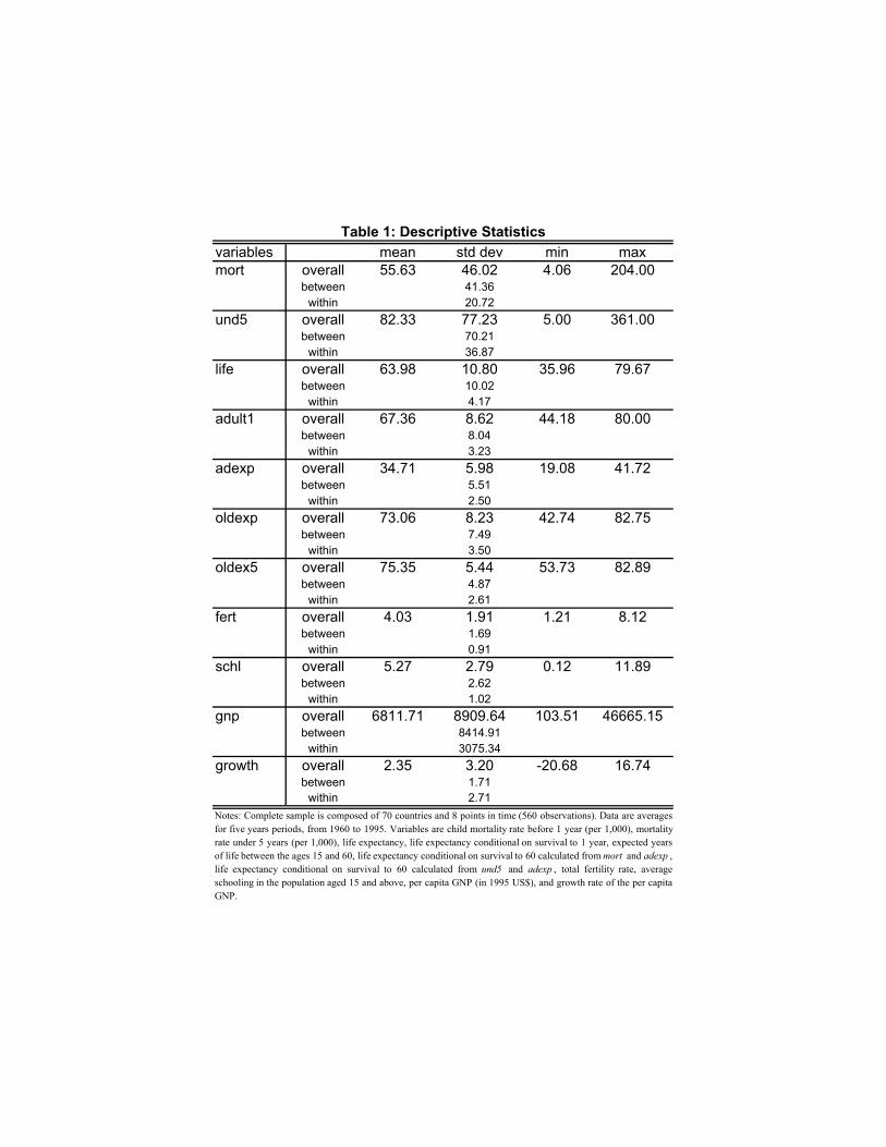
variables mean std dev min maxmort overall 55.63 46.02 4.06 204.00
between 41.36within 20.72
und5 overall 82.33 77.23 5.00 361.00between 70.21
within 36.87life overall 63.98 10.80 35.96 79.67
between 10.02within 4.17
adult1 overall 67.36 8.62 44.18 80.00between 8.04
within 3.23adexp overall 34.71 5.98 19.08 41.72
between 5.51within 2.50
oldexp overall 73.06 8.23 42.74 82.75between 7.49
within 3.50oldex5 overall 75.35 5.44 53.73 82.89
between 4.87within 2.61
fert overall 4.03 1.91 1.21 8.12between 1.69
within 0.91schl overall 5.27 2.79 0.12 11.89
between 2.62within 1.02
gnp overall 6811.71 8909.64 103.51 46665.15between 8414.91
within 3075.34growth overall 2.35 3.20 -20.68 16.74
between 1.71within 2.71
Table 1: Descriptive Statistics
Notes: Complete sample is composed of 70 countries and 8 points in time (560 observations). Data are averagesfor five years periods, from 1960 to 1995. Variables are child mortality rate before 1 year (per 1,000), mortalityrate under 5 years (per 1,000), life expectancy, life expectancy conditional on survival to 1 year, expected yearsof life between the ages 15 and 60, life expectancy conditional on survival to 60 calculated frommort and adexp , life expectancy conditional on survival to 60 calculated from und5 and adexp , total fertility rate, averageschooling in the population aged 15 and above, per capita GNP (in 1995 US$), and growth rate of the per capitaGNP.
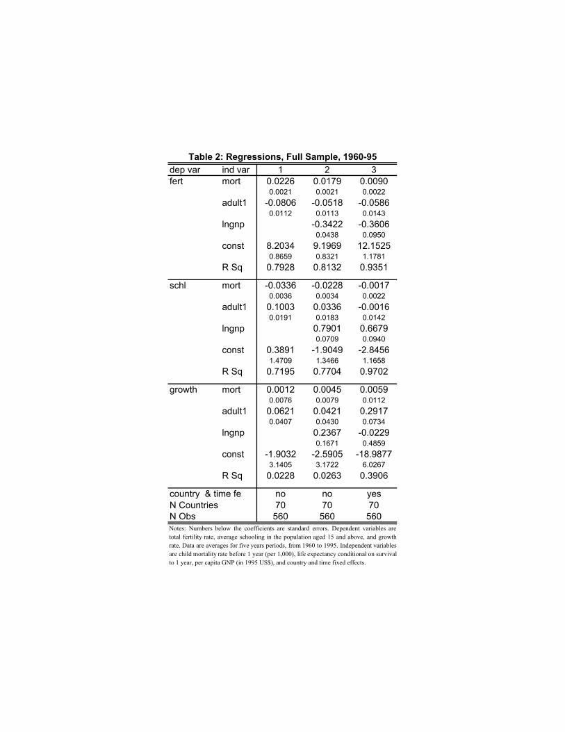
dep var ind var 1 2 3fert mort 0.0226 0.0179 0.0090
0.0021 0.0021 0.0022adult1 -0.0806 -0.0518 -0.0586
0.0112 0.0113 0.0143lngnp -0.3422 -0.3606
0.0438 0.0950const 8.2034 9.1969 12.1525
0.8659 0.8321 1.1781R Sq 0.7928 0.8132 0.9351
schl mort -0.0336 -0.0228 -0.00170.0036 0.0034 0.0022
adult1 0.1003 0.0336 -0.00160.0191 0.0183 0.0142
lngnp 0.7901 0.66790.0709 0.0940
const 0.3891 -1.9049 -2.84561.4709 1.3466 1.1658
R Sq 0.7195 0.7704 0.9702
growth mort 0.0012 0.0045 0.00590.0076 0.0079 0.0112
adult1 0.0621 0.0421 0.29170.0407 0.0430 0.0734
lngnp 0.2367 -0.02290.1671 0.4859
const -1.9032 -2.5905 -18.98773.1405 3.1722 6.0267
R Sq 0.0228 0.0263 0.3906
no no yesN Countries 70 70 70N Obs 560 560 560
Table 2: Regressions, Full Sample, 1960-95
Notes: Numbers below the coefficients are standard errors. Dependent variables aretotal fertility rate, average schooling in the population aged 15 and above, and growthrate. Data are averages for five years periods, from 1960 to 1995. Independent variablesare child mortality rate before 1 year (per 1,000), life expectancy conditional on survivalto 1 year, per capita GNP (in 1995 US$), and country and time fixed effects.
country & time fe

fert schl growth0.0201 0.0029 0.01960.0028 0.0039 0.0158
-0.1653 0.0675 0.45720.0192 0.0269 0.1104
0.1585 0.4881 -0.60290.1134 0.1585 0.6509yes yes yes
0.9333 0.9478 0.397247 47 47376 376 376
fert schl growth fert schl growth fert schl growthchild mort 0.0213 0.0022 0.0146 0.0144 0.0003 0.0002 -0.0036 0.0237 -0.0230
0.0036 0.0054 0.0199 0.0020 0.0030 0.0112 0.0135 0.0195 0.0831adult exp -0.2092 0.1211 0.4412 -0.1847 0.0662 0.5973 -0.4933 0.4863 -0.2588
0.0344 0.0519 0.1918 0.0329 0.0483 0.1826 0.2045 0.2954 1.2584old age exp -0.0129 -0.0322 0.3352 -0.0174 -0.0755 0.0321
0.0462 0.0696 0.2572 0.0426 0.0625 0.2362lngnp 0.1079 0.5935 -0.9545 0.3008 0.2712 -1.0717 0.7367 -0.1665 1.1785
0.1331 0.2006 0.7417 0.1493 0.2191 0.8277 0.3963 0.5736 2.4384country & time fe yes yes yes yes yes yes yes yes yesR Sq 0.9323 0.9409 0.4616 0.9334 0.9457 0.4643N Countries 46 46 46 41 41 41 40 40 40N Obs 230 230 230 205 205 205 155 155 155
Table 4: Robustness Check, Regressions with Different Age Specific Mortality Rates or with Instrument, Selected Sample - "Post-transition" Countries, 1960-95
Notes: Numbers below the coefficients are standard errors. Only countries with life expectancy at birth in 1960 above 50 years included. Dependent variables are total fertilityrate, average schooling in the population aged 15 and above, and growth rate. For the regressions including old age life expectancy (columns 1-6), data are averages for five yearperiods, for the years 1960, 70, 80, 90, and 95. For the instrumental variable regression (columns 7-9), data are averages for five year periods, for the years 1970-95 (unbalancedpanel). Independent variables for columns 1-3 are child mortality rate before 1 year (per 1,000), expected years of adult life, and life expectancy conditional on survival to 60.Independent variables for columns 4-6 are child mortality rate before 5 years (per 1,000), expected years of adult life, and life expectancy conditional on survival to 60.Independent variables for columns 7-9 are child mortality rate before 1 year (per 1,000) and life expectancy conditional on survival to 1 (instrument: % of population with accessto safe water). All include per capita GNP (in 1995 US$), and country and time fixed effects.
child mortality before 1 child mortality before 5 IV
Notes: Numbers below the coefficients are standard errors. Only countries withlife expectancy at birth above 50 in 1960 included in the regressions. Dependentvariables are total fertility rate, average schooling in the population aged 15 andabove, and growth rate. Data are averages for five years periods, from 1960 to1995. Independent variables are child mortality rate before 1 year before 1 yearper (1,000), life expectancy conditional on survival to 1 year, per capita GNP (in1995 US$), and country and time fixed effects.
Table 3: Regression, Selected Sample - "Post-transition" Countries, 1960-95
mort
adult1
lngnp
country & time feR SqN CountriesN Obs
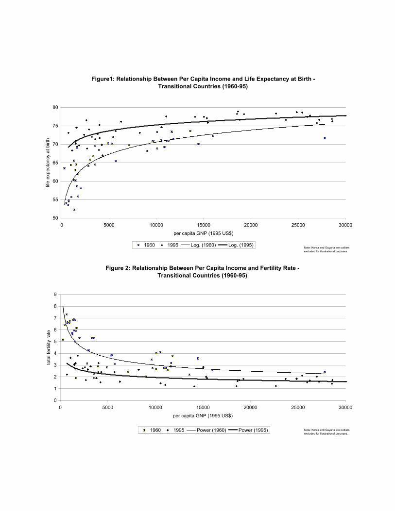
Figure1: Relationship Between Per Capita Income and Life Expectancy at Birth -Transitional Countries (1960-95)
50
55
60
65
70
75
80
0 5000 10000 15000 20000 25000 30000per capita GNP (1995 US$)
life
expe
ctan
cy a
t birt
h
1960 1995 Log. (1960) Log. (1995)Note: Korea and Guyana are outliers excluded for illustrational purposes.
Figure 2: Relationship Between Per Capita Income and Fertility Rate -Transitional Countries (1960-95)
0
1
2
3
4
5
6
7
8
9
0 5000 10000 15000 20000 25000 30000per capita GNP (1995 US$)
tota
l fer
tility
rate
1960 1995 Power (1960) Power (1995) Note: Korea and Guyana are outliers excluded for illustrational purposes.
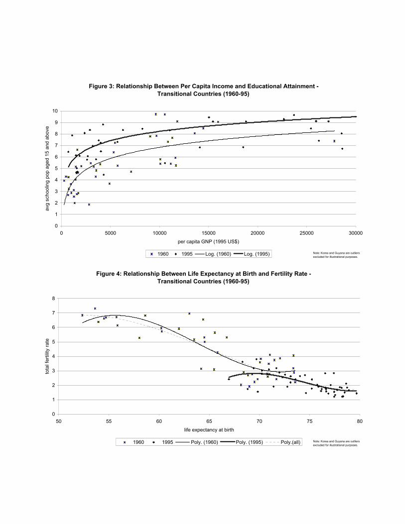
Figure 3: Relationship Between Per Capita Income and Educational Attainment -Transitional Countries (1960-95)
0
1
2
3
4
5
6
7
8
9
10
0 5000 10000 15000 20000 25000 30000per capita GNP (1995 US$)
avg
scho
olin
g po
p ag
ed 1
5 an
d ab
ove
1960 1995 Log. (1960) Log. (1995) Note: Korea and Guyana are outliers excluded for illustrational purposes.
Figure 4: Relationship Between Life Expectancy at Birth and Fertility Rate -Transitional Countries (1960-95)
0
1
2
3
4
5
6
7
8
50 55 60 65 70 75 80life expectancy at birth
tota
l fer
tility
rate
1960 1995 Poly. (1960) Poly. (1995) Poly.(all) Note: Korea and Guyana are outliers excluded for illustrational purposes.
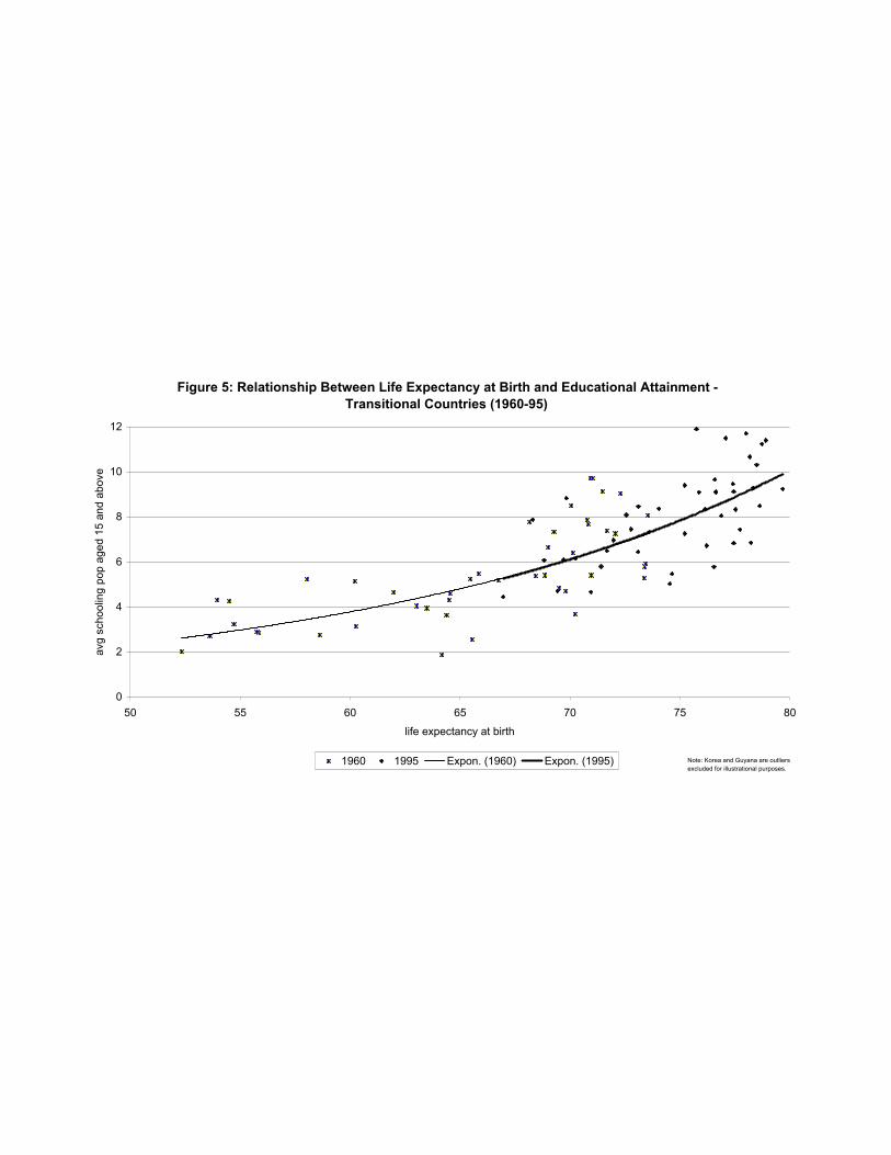
Figure 5: Relationship Between Life Expectancy at Birth and Educational Attainment -Transitional Countries (1960-95)
0
2
4
6
8
10
12
50 55 60 65 70 75 80life expectancy at birth
avg
scho
olin
g po
p ag
ed 1
5 an
d ab
ove
1960 1995 Expon. (1960) Expon. (1995) Note: Korea and Guyana are outliers excluded for illustrational purposes.
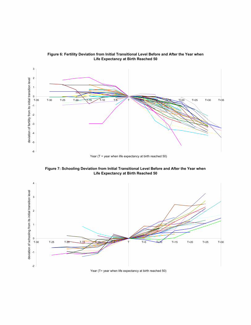
Figure 6: Fertility Deviation from Initial Transitional Level Before and After the Year when Life Expectancy at Birth Reached 50
-6
-5
-4
-3
-2
-1
0
1
2
3
T-35 T-30 T-25 T-20 T-15 T-10 T-5 T T+5 T+10 T+15 T+20 T+25 T+30 T+35
Year (T = year when life expectancy at birth reached 50)
devi
atio
n of
ferti
lity
from
its
initi
al tr
ansi
tion
leve
l
Figure 7: Schooling Deviation from Initial Transitional Level Before and After the Year when Life Expectancy at Birth Reached 50
-2
-1
0
1
2
3
4
T-30 T-25 T-20 T-15 T-10 T-5 T T+5 T+10 T+15 T+20 T+25 T+30
Year (T= year when life expectancy at birth reached 50)
devi
atio
n of
sch
oolin
g fro
m it
s in
itial
tran
sitio
n le
vel
Related Documents