Monroe L. Weber- Shirk School of Civil and Environmental Engineering Basic Governing Differential Equations CEE 331 March 16, 2022

Monroe L. Weber-Shirk S chool of Civil and Environmental Engineering Basic Governing Differential Equations CEE 331 July 14, 2015 CEE 331 July 14, 2015.
Dec 22, 2015
Welcome message from author
This document is posted to help you gain knowledge. Please leave a comment to let me know what you think about it! Share it to your friends and learn new things together.
Transcript
Monroe L. Weber-Shirk School of Civil and
Environmental Engineering
Basic Governing Differential Equations
Basic Governing Differential Equations
CEE 331
April 19, 2023
CEE 331
April 19, 2023
OverviewOverview
Continuity Equation Navier-Stokes Equation
(a bit of vector notation...) Examples (all laminar flow)
Flow between stationary parallel horizontal plates
Flow between inclined parallel plates Pipe flow (Hagen Poiseuille)
Continuity Equation Navier-Stokes Equation
(a bit of vector notation...) Examples (all laminar flow)
Flow between stationary parallel horizontal plates
Flow between inclined parallel plates Pipe flow (Hagen Poiseuille)
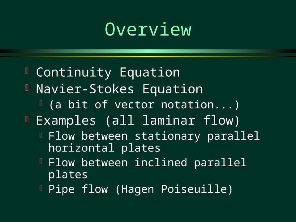
Why Differential Equations? Why Differential Equations?
A droplet of water Clouds Wall jet Hurricane
A droplet of water Clouds Wall jet Hurricane
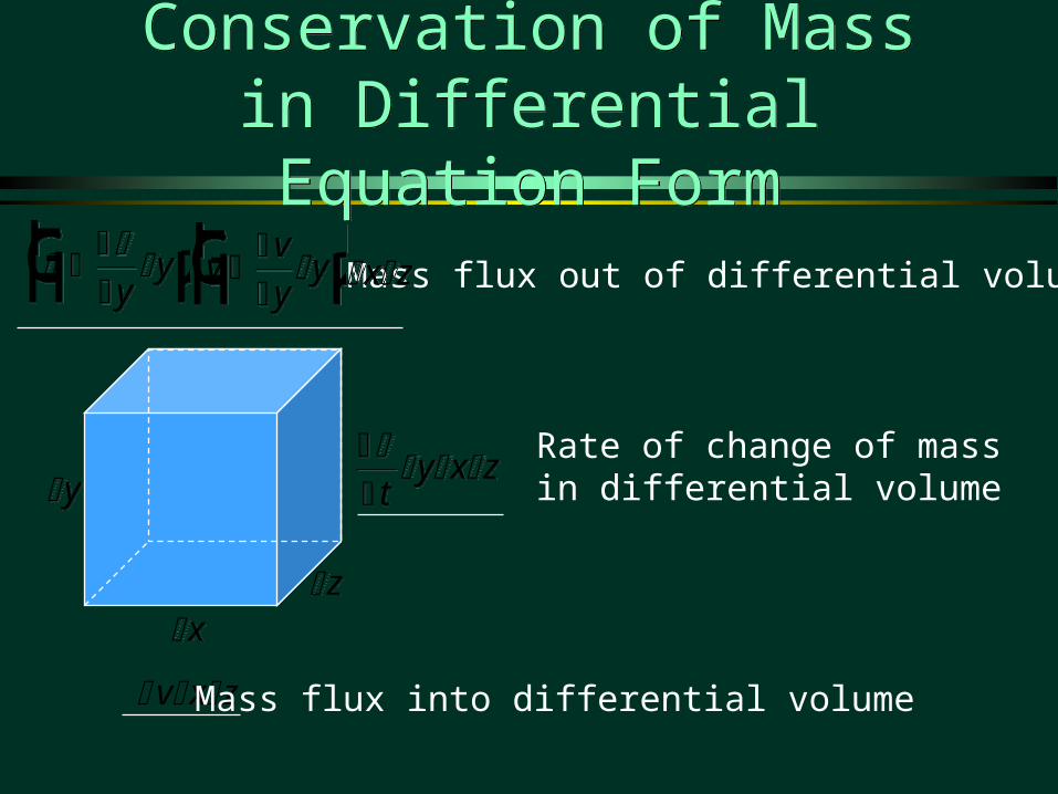
Conservation of Mass in Differential Equation Form
Conservation of Mass in Differential Equation Form
v x z
xx
yy
z z
FHG
IKJy
y
FHG
IKJy
y
t
y x z t
y x z
Mass flux into differential volume
Mass flux out of differential volume
Rate of change of mass in differential volume
vvy
y
FHG
IKJv
vy
y
FHG
IKJ x z x z

Continuity EquationContinuity Equation
vy
vy t
vy
vy t
Mass flux out of differential volume
vvy
y vy
yvy y
y x z
FHG
IKJ
2 vvy
y vy
yvy y
y x z
FHG
IKJ
2 Higher order termHigher order term
outout inin Rate of mass decreaseRate of mass decrease
vy t
0
vy t
0 1-d continuity equation1-d continuity equation
vvy
y vy
y x z v x zt
y x z
FHG
IKJ
vvy
y vy
y x z v x zt
y x z
FHG
IKJ
u, v, w are velocities in x, y, and z directions
u, v, w are velocities in x, y, and z directions
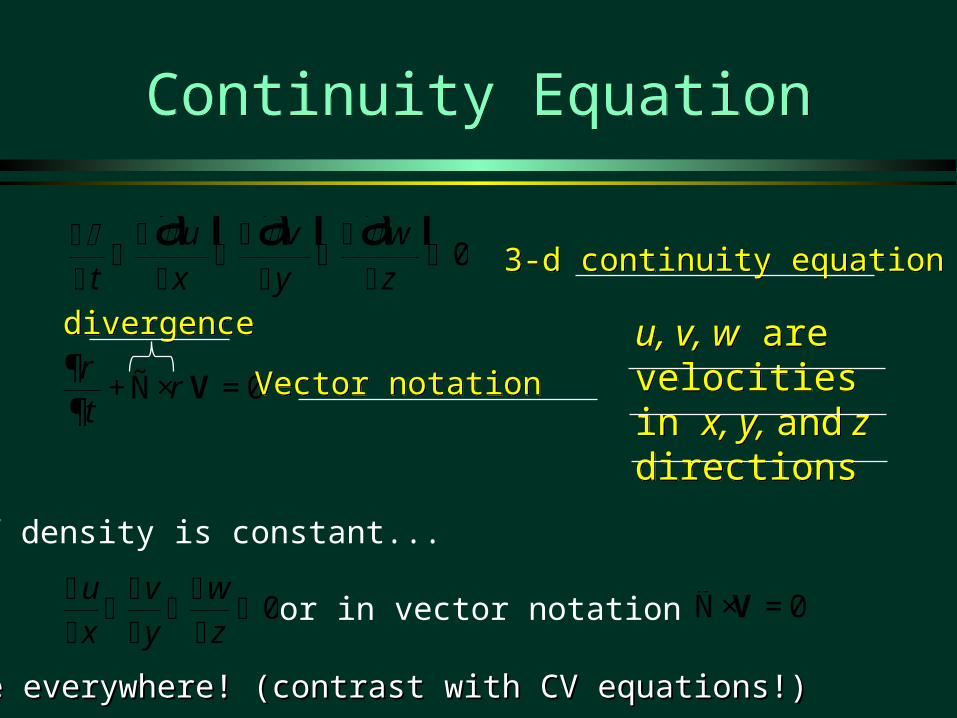
Continuity EquationContinuity Equation
0tr
r
+Ñ× =
V
t
u
x
v
y
w
z
af af a f0 3-d continuity equation3-d continuity equation
If density is constant...
ux
vy
wz
0
Vector notationVector notation
0Ñ× =Vor in vector notation
True everywhere! (contrast with CV equations!)True everywhere! (contrast with CV equations!)
divergencedivergence
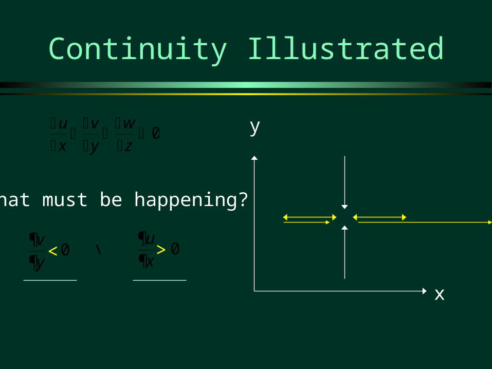
Continuity IllustratedContinuity Illustrated
ux
vy
wz
0
x
y
What must be happening?
0vy¶¶
0ux¶¶
\< >
ShearShear
GravityGravityPressurePressure
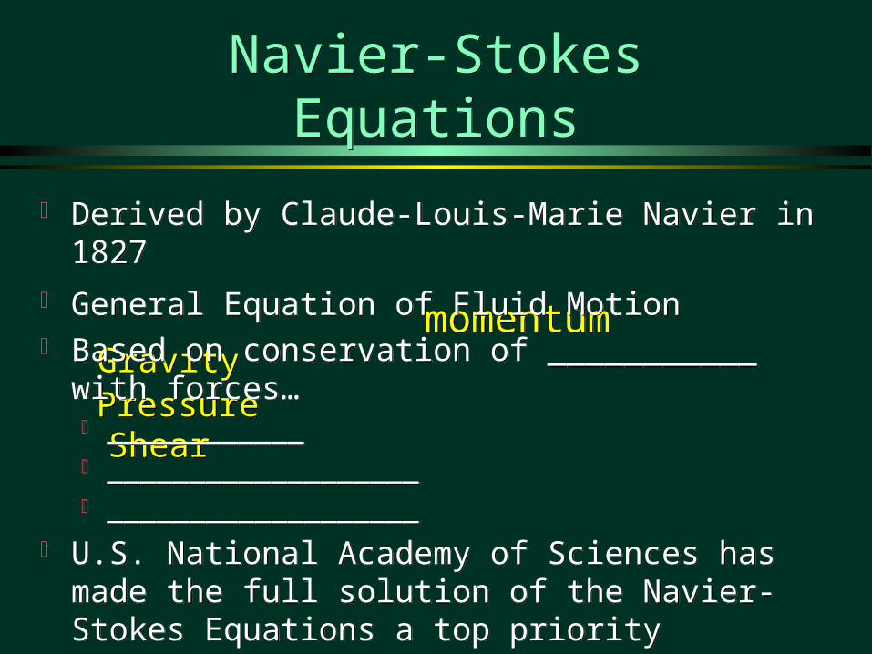
Navier-Stokes EquationsNavier-Stokes Equations
momentummomentum
Derived by Claude-Louis-Marie Navier in 1827
General Equation of Fluid Motion Based on conservation of ___________ with forces…
____________ ___________________ ___________________
U.S. National Academy of Sciences has made the full solution of the Navier-Stokes Equations a top priority
Derived by Claude-Louis-Marie Navier in 1827
General Equation of Fluid Motion Based on conservation of ___________ with forces…
____________ ___________________ ___________________
U.S. National Academy of Sciences has made the full solution of the Navier-Stokes Equations a top priority
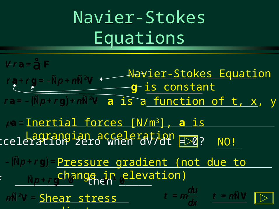
If _________ then _____
Navier-Stokes Equation
Inertial forces [N/m3], a is Lagrangian acceleration
Pressure gradient (not due to change in elevation)
Shear stress gradient
Navier-Stokes EquationsNavier-Stokes Equations
V r =åa FV r =åa F2pa g Vr r m+ =-Ñ + Ñ2pa g Vr r m+ =-Ñ + Ñ
a a
( )p gr- Ñ + =( )p gr- Ñ + =
2mÑ =V2mÑ =Vdudx
t m=dudx
t m=
Is acceleration zero when dV/dt = 0?
t m= ÑVt m= ÑV
( ) 2pa g Vr r m=- Ñ + + Ñ( ) 2pa g Vr r m=- Ñ + + Ñg is constanta is a function of t, x, y, z
NO!
0p rÑ + ¹g 0p rÑ + ¹g 0V ¹ 0V ¹

Lagrangian accelerationLagrangian acceleration
Notation: Total DerivativeEulerian Perspective
Notation: Total DerivativeEulerian Perspective
u v wt x y z
¶ ¶ ¶ ¶= + + +¶ ¶ ¶ ¶V V V V
a u v wt x y z
¶ ¶ ¶ ¶= + + +¶ ¶ ¶ ¶V V V V
a
( , , , )D
t x y z u v wDt t x y za a a a a¶ ¶ ¶ 
= + + +¶ ¶ ¶ 
( , , , )D
t x y z u v wDt t x y za a a a a¶ ¶ ¶ 
= + + +¶ ¶ ¶ 
( , , , )D
t x y z u v wDt t x y z
¶ ¶ ¶ ¶= + + +¶ ¶ ¶ 
V V V V V( , , , )
Dt x y z u v w
Dt t x y z¶ ¶ ¶ 
= + + +¶ ¶ ¶ 
V V V V V
tV
a V V
= + ×ѶtV
a V V
= + ×Ѷ
kjizyx
()()()
() kjizyx
()()()
()
( ) () () ()() u v w
x y z¶ ¶ 
×Ñ = + +¶ ¶ 
V( ) () () ()() u v w
x y z¶ ¶ 
×Ñ = + +¶ ¶ 
V
( , , , )D dt dx dy dz
t x y zDt t dt x dt y dt z dta a a a a¶ ¶ ¶ 
= + + +¶ ¶ ¶ 
( , , , )D dt dx dy dz
t x y zDt t dt x dt y dt z dta a a a a¶ ¶ ¶ 
= + + +¶ ¶ ¶ 
Total derivative (chain rule)
Material or substantial derivative

x2 1VVV =D - =2 1VVV =D - =
tV
a V V
= + ×ѶtV
a V V
= + ×Ѷ
Over what time did this change of velocity occur (for a particle of fluid)? x
tVD
D =x
tVD
D =
space tV
a =DD
=space tV
a =DD
=V
Vx
DDV
Vx
DD
1V1V 2V2V
VDVD
111111 VVM QAV 111111 VVM QAV
222222 VVM QAV 222222 VVM QAV
( )1 2 AVM M Vr+ = D( )1 2 AVM M Vr+ = D
Why no term?tV¶¶tV¶¶
N-S
Application of Navier-Stokes Equations
Application of Navier-Stokes Equations
The equations are nonlinear partial differential equations
No full analytical solution exists The equations can be solved for several
simple flow conditions Numerical solutions to Navier-Stokes
equations are increasingly being used to describe complex flows.
The equations are nonlinear partial differential equations
No full analytical solution exists The equations can be solved for several
simple flow conditions Numerical solutions to Navier-Stokes
equations are increasingly being used to describe complex flows.
( )0 p gr=- Ñ +( )0 p gr=- Ñ +
Navier-Stokes Equations: A Simple Case
Navier-Stokes Equations: A Simple Case
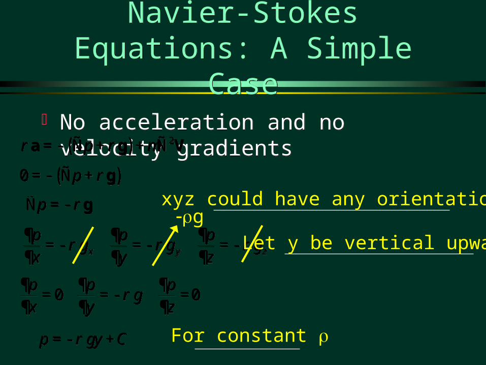
No acceleration and no velocity gradients No acceleration and no velocity gradients
p gy Cr=- +p gy Cr=- +
p grÑ =-p grÑ =-
x y z
p p pg g g
x y zr r r
¶ ¶ ¶=- =- =-
¶ ¶ ¶x y z
p p pg g g
x y zr r r
¶ ¶ ¶=- =- =-
¶ ¶ 
0 0p p p
gx y z
r¶ ¶ 
= =- =¶ ¶ 
0 0p p p
gx y z
r¶ ¶ 
= =- =¶ ¶ 
xyz could have any orientation
Let y be vertical upward
g
For constant
( ) 2pa g Vr r m=- Ñ + + Ñ( ) 2pa g Vr r m=- Ñ + + Ñ
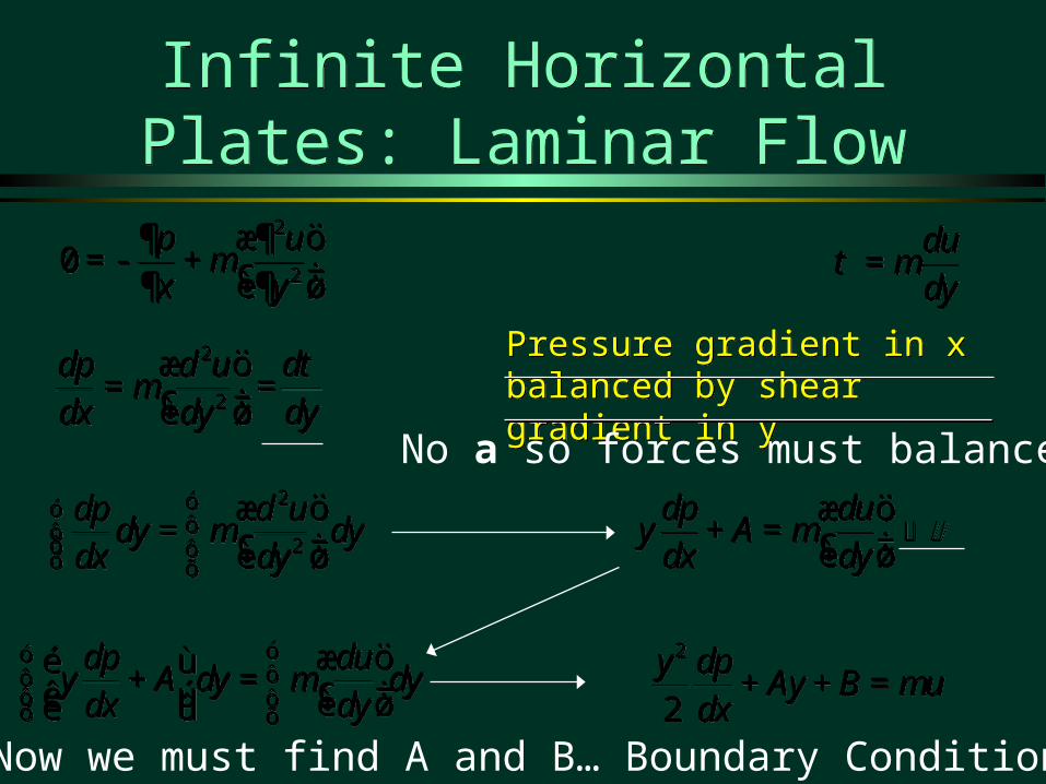
Infinite Horizontal Plates: Laminar Flow
Infinite Horizontal Plates: Laminar Flow
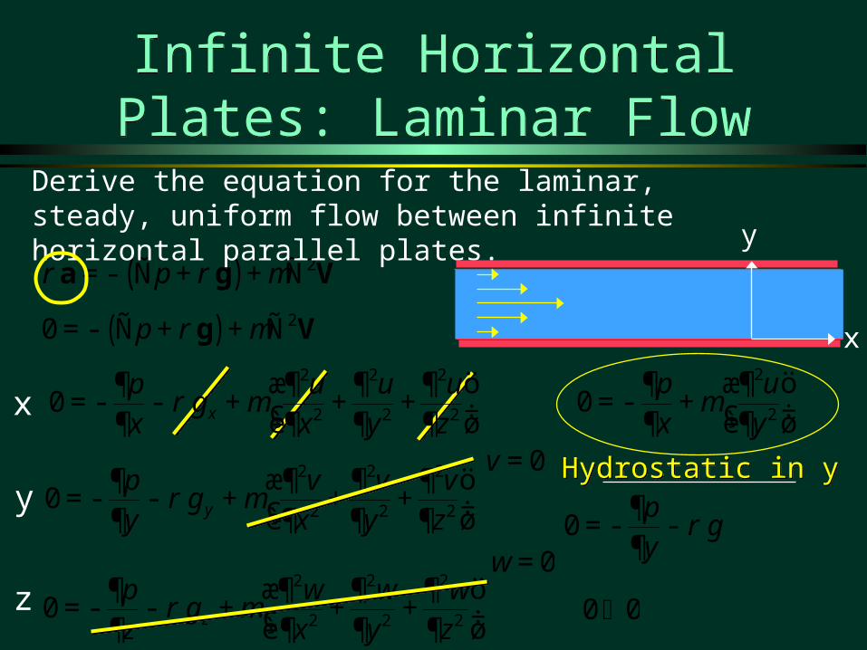
( ) 2pa g Vr r m=- Ñ + + Ñ
( ) 20 p g Vr m=- Ñ + + Ñ
Derive the equation for the laminar, steady, uniform flow between infinite horizontal parallel plates.
2
20p ux y
mæ ö¶ 
=- + ç ÷è ø¶ 
0p
gy
r
=- -
0 0
2 2 2
2 2 20 y
p v v vg
y x y zr m
æ ö¶ ¶ ¶ ¶=- - + + +ç ÷è ø¶ ¶ ¶ 
2 2 2
2 2 20 z
p w w wg
z x y zr m
æ ö¶ ¶ ¶ ¶=- - + + +ç ÷è ø¶ ¶ ¶ 
2 2 2
2 2 20 x
p u u ug
x x y zr m
æ ö¶ ¶ ¶ ¶=- - + + +ç ÷è ø¶ ¶ ¶ 
y
x
Hydrostatic in yHydrostatic in y0v =
0w =
x
y
z
Infinite Horizontal Plates: Laminar Flow
Infinite Horizontal Plates: Laminar Flow
2
20p ux y
mæ ö¶ 
=- + ç ÷è ø¶ 
2
20p ux y
mæ ö¶ 
=- + ç ÷è ø¶ 
2
2
dp d udx dy
mæ ö
= ç ÷è ø
2
2
dp d udx dy
mæ ö
= ç ÷è ø
2
2
dp d udy dy
dx dym
óóôôô ôõ õ
æ ö= ç ÷è ø
2
2
dp d udy dy
dx dym
óóôôô ôõ õ
æ ö= ç ÷è ø
dp duy A
dx dymæ ö
+ = ç ÷è ødp du
y Adx dy
mæ ö
+ = ç ÷è ø
dp duy A dy dy
dx dym
óóôô
ô ôõ õ
æ öé ù+ = ç ÷ê ú è øë û
dp duy A dy dy
dx dym
óóôô
ô ôõ õ
æ öé ù+ = ç ÷ê ú è øë û
2
2y dp
Ay B udx
m+ + =2
2y dp
Ay B udx
m+ + =
Pressure gradient in x balanced by shear gradient in yPressure gradient in x balanced by shear gradient in y
dudy
t m=dudy
t m=
ddyt
=ddyt
=
No a so forces must balance!
Now we must find A and B… Boundary Conditions

negativenegative
Infinite Horizontal Plates: Boundary Conditions
Infinite Horizontal Plates: Boundary Conditions
No slip condition
u = 0 at y = 0 and y = au = 0 at y = 0 and y = a a
B 0
a dpdx
Aa2
20 A
a dpdx
2
( )2
y y a dpu
dxm-
=2a dp
ydx
t æ ö= -è ø2
a dpy
dxt æ ö= -
è ø
y
du dpy A
dy dxmæ ö
= +ç ÷è ødu dp
y Ady dx
mæ ö
= +ç ÷è ø
dpdx
dpdx
let be___________
uu
2
2y dp
Ay B udx
m+ + =
What can we learn about ?
x
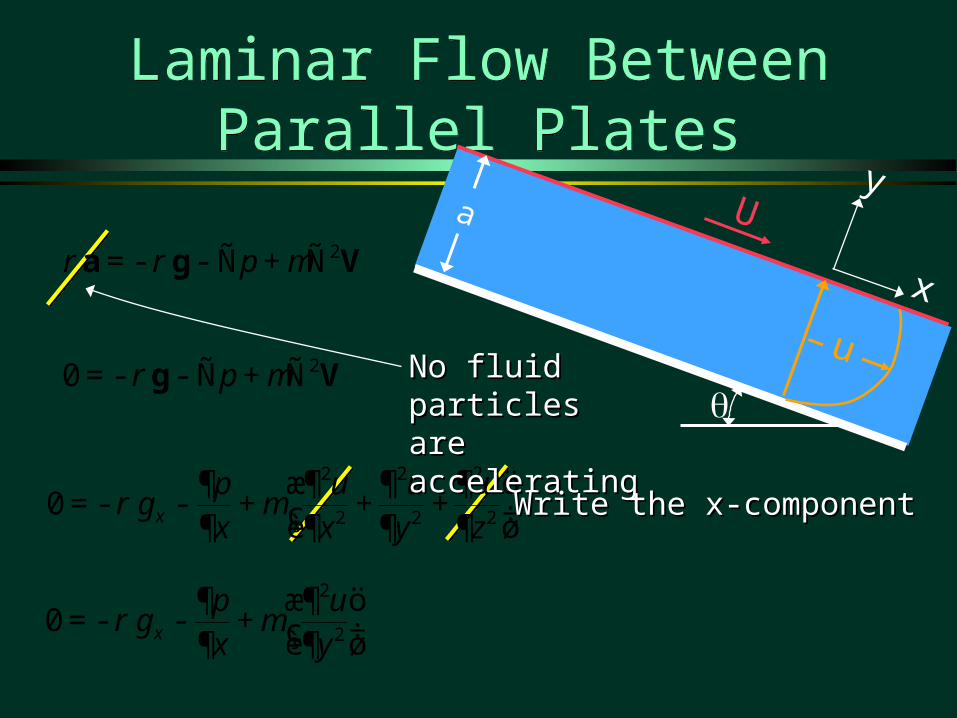
Laminar Flow Between Parallel Plates
Laminar Flow Between Parallel Plates
2pa g Vr r m=- - Ñ + Ñ
20 pg Vr m=- - Ñ + Ñ
2
20 x
p ug
x yr m
æ ö¶ ¶=- - + ç ÷è ø¶ 
2 2 2
2 2 20 x
p u u ug
x x y zr m
æ ö¶ ¶ ¶ ¶=- - + + +ç ÷è ø¶ ¶ ¶ 
U
a
u
y
x
No fluid particles No fluid particles are acceleratingare accelerating
Write the x-componentWrite the x-component
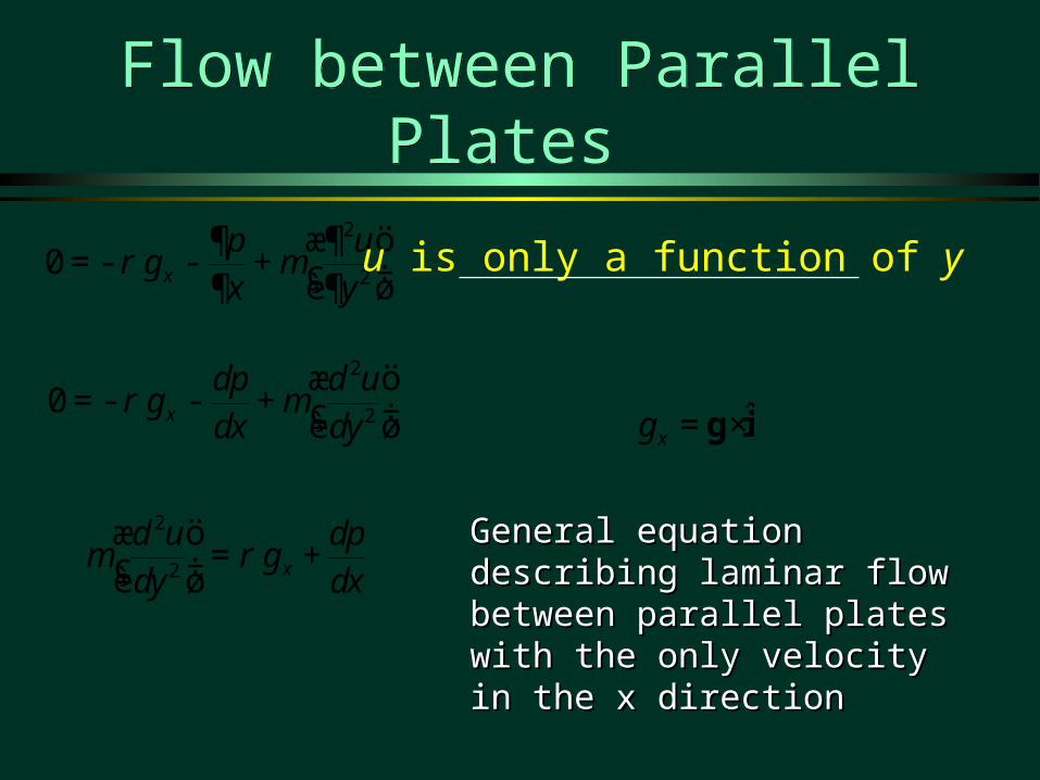
Flow between Parallel Plates Flow between Parallel Plates
2
20 x
p ug
x yr m
æ ö¶ ¶=- - + ç ÷è ø¶ 
2
20 x
dp d ug
dx dyr m
æ ö=- - + ç ÷è ø
General equation describing laminar General equation describing laminar flow between parallel plates with the flow between parallel plates with the only velocity in the x directiononly velocity in the x direction
u is only a function of y
ˆxg g i= ×
2
2 x
d u dpg
dy dxm ræ ö
= +ç ÷è ø

Flow Between Parallel Plates: Integration
Flow Between Parallel Plates: Integration
2
2 x
d u dpg
dy dxm r= +
2
2 x
d u dpg
dy dxm r= +
x
du dpy g A
dy dxm ræ ö= + + =
è øx
du dpy g A
dy dxm ræ ö= + + =
è ø
2
2 x
d u dpdy g dy
dy dxm ræ ö= +
è øó ó
ôôõõ
2
2 x
d u dpdy g dy
dy dxm ræ ö= +
è øó ó
ôôõõ
x
du dpdy y g A dy
dy dxm ræ öæ ö= + +ç ÷è øè ø
óóô ôõ õ
x
du dpdy y g A dy
dy dxm ræ öæ ö= + +ç ÷è øè ø
óóô ôõ õ
2
2 x
y dpu g Ay B
dxm ræ ö= + + +
è ø
2
2 x
y dpu g Ay B
dxm ræ ö= + + +
è ø
U
a
u
y
x
tt

u = U at y = a
Boundary ConditionsBoundary Conditions
2
2 x
y dpu g Ay B
dxm ræ ö= + + +
è ø
2
2 x
y dpu g Ay B
dxm ræ ö= + + +
è ø
Boundary condition
B 000 B 000
Boundary condition
2
2 x
a dpU g Aa
dxm ræ ö= + +
è ø
2
2 x
a dpU g Aa
dxm ræ ö= + +
è ø 2 x
U a dpA g
a dxm
ræ ö= - +è ø2 x
U a dpA g
a dxm
ræ ö= - +è ø
2
2 x
Uy y ay dpu g
a dxr
m- æ ö= + +
è ø
2
2 x
Uy y ay dpu g
a dxr
m- æ ö= + +
è ø
u = 0 at y = 0
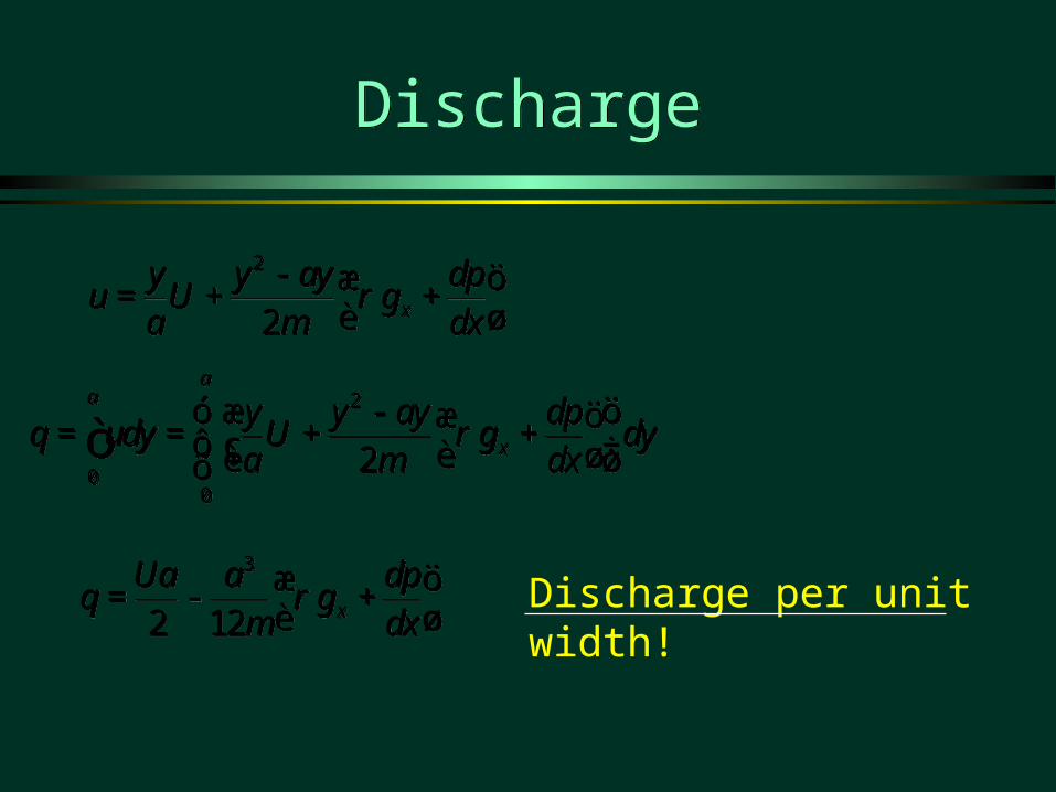
Discharge per unit width!
DischargeDischarge
2
00
2
aa
x
y y ay dpq udy U g dy
a dxr
mæ ö- æ ö= = + +ç ÷è øè ø
óôõ
ò2
00
2
aa
x
y y ay dpq udy U g dy
a dxr
mæ ö- æ ö= = + +ç ÷è øè ø
óôõ
ò
3
2 12 x
Ua a dpq g
dxr
mæ ö= - +è ø
3
2 12 x
Ua a dpq g
dxr
mæ ö= - +è ø
2
2 x
y y ay dpu U g
a dxr
m- æ ö= + +
è ø
2
2 x
y y ay dpu U g
a dxr
m- æ ö= + +
è ø
Example: Oil SkimmerExample: Oil Skimmer
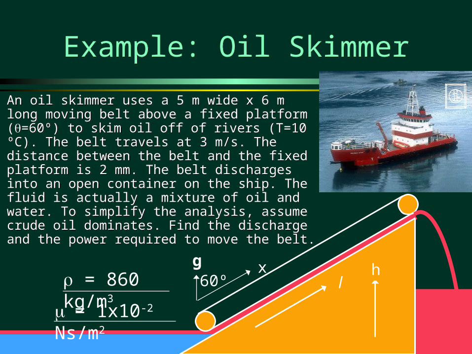
An oil skimmer uses a 5 m wide x 6 m long moving belt above a fixed platform (=60º) to skim oil off of rivers (T=10 ºC). The belt travels at 3 m/s. The distance between the belt and the fixed platform is 2 mm. The belt discharges into an open container on the ship. The fluid is actually a mixture of oil and water. To simplify the analysis, assume crude oil dominates. Find the discharge and the power required to move the belt.
An oil skimmer uses a 5 m wide x 6 m long moving belt above a fixed platform (=60º) to skim oil off of rivers (T=10 ºC). The belt travels at 3 m/s. The distance between the belt and the fixed platform is 2 mm. The belt discharges into an open container on the ship. The fluid is actually a mixture of oil and water. To simplify the analysis, assume crude oil dominates. Find the discharge and the power required to move the belt.
hl
= 1x10⁻² Ns/m2
= 860 kg/m3 60ºxg
Example: Oil SkimmerExample: Oil Skimmer
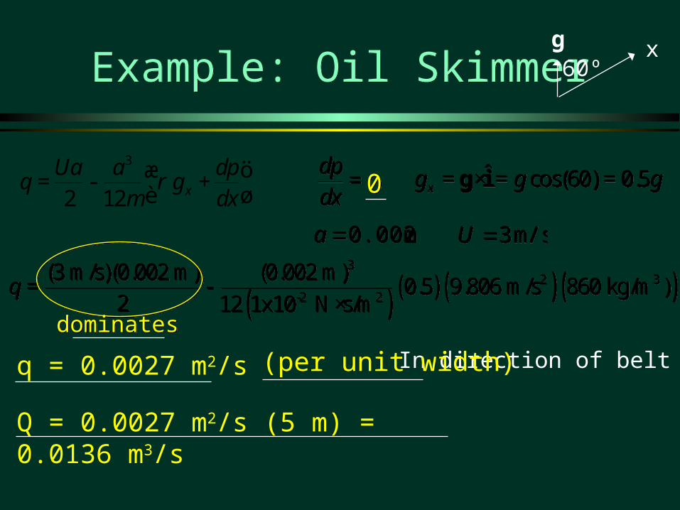
dpdx
=dpdx
= ˆ cos(60) 0.5xg g g= ×= =g i cos(60) 0.5xg g g= ×= =g i
m 0.002a m 0.002a m/s 3U m/s 3U
( ) ( ) ( ) ( )3
2 3-2 2
(3 m/s)(0.002 m) (0.002 m)0.5 9.806 m/s 860 kg/m )
2 12 1x10 N s/mq = -
×( ) ( ) ( ) ( )3
2 3-2 2
(3 m/s)(0.002 m) (0.002 m)0.5 9.806 m/s 860 kg/m )
2 12 1x10 N s/mq = -
×
In direction of beltq = 0.0027 m2/s (per unit width)
Q = 0.0027 m2/s (5 m) = 0.0136 m3/s
3
2 12 x
Ua a dpq g
dxr
mæ ö= - +è ø 00
dominatesdominates
60ºxg
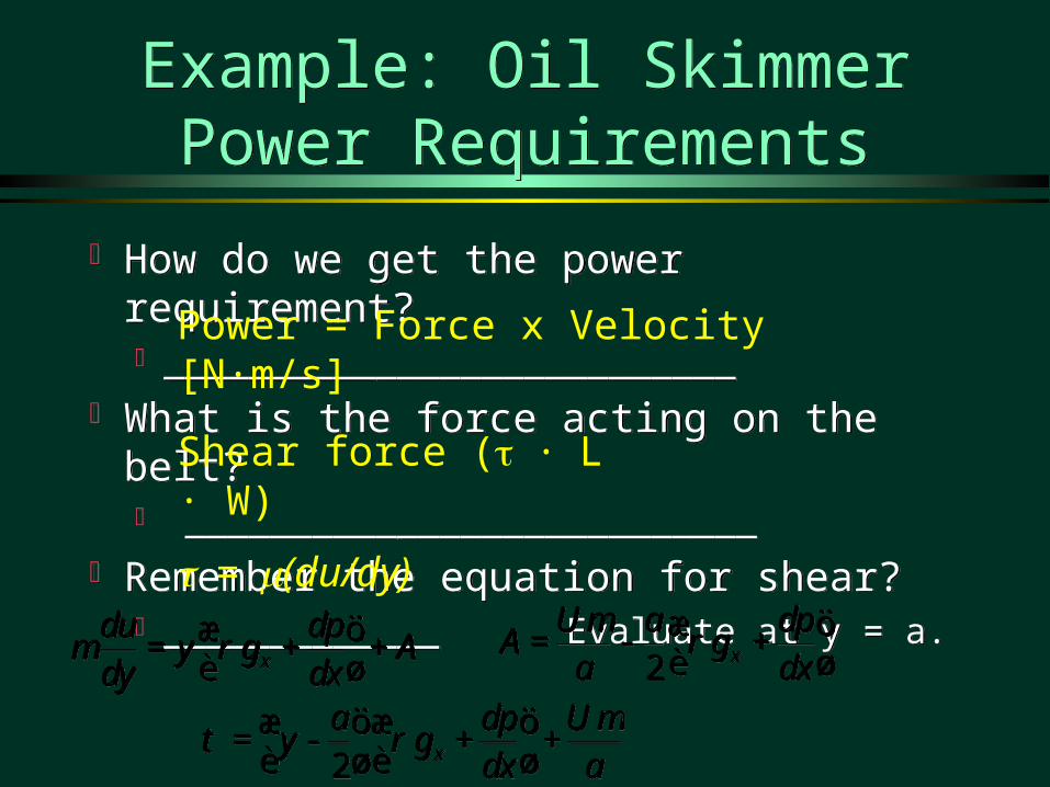
How do we get the power requirement? ___________________________
What is the force acting on the belt? ___________________________
Remember the equation for shear? _____________ Evaluate at y = a.
How do we get the power requirement? ___________________________
What is the force acting on the belt? ___________________________
Remember the equation for shear? _____________ Evaluate at y = a.
Example: Oil Skimmer Power Requirements
Example: Oil Skimmer Power Requirements
x
du dpy g A
dy dxm ræ ö= + +
è øx
du dpy g A
dy dxm ræ ö= + +
è ø 2 x
U a dpA g
a dxm
ræ ö= - +è ø2 x
U a dpA g
a dxm
ræ ö= - +è ø
2 x
a dp Uy g
dx am
t ræ öæ ö= - + +è øè ø2 x
a dp Uy g
dx am
t ræ öæ ö= - + +è øè ø
Power = Force x Velocity [N·m/s]
Shear force (·L · W)
=(du/dy)
Example: Oil Skimmer Power Requirements
Example: Oil Skimmer Power Requirements
2 x
a dp Uy g
dx am
t ræ öæ ö= - + +è øè ø2 x
a dp Uy g
dx am
t ræ öæ ö= - + +è øè ø
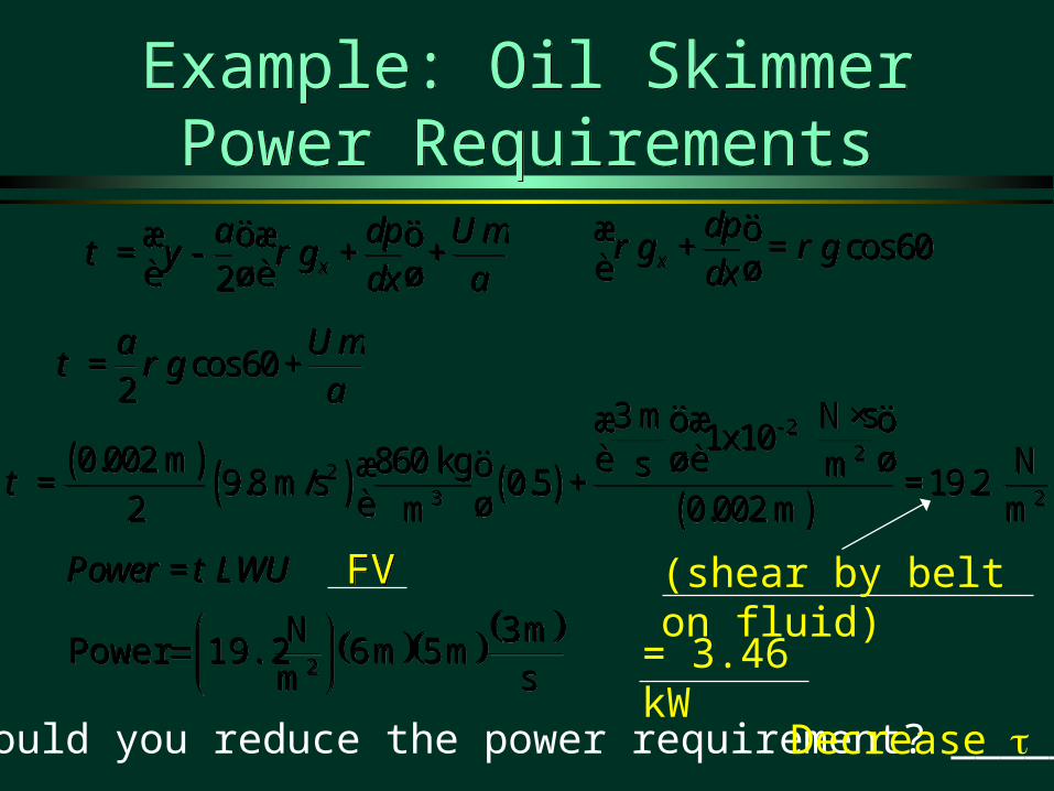
cos 602a U
gam
t r= +cos 602a U
gam
t r= +
cos 60x
dpg g
dxr ræ ö+ =è ø
cos 60x
dpg g
dxr ræ ö+ =è ø
( ) ( ) ( )( )
22
23 2
3 m N s1x10
0.002 m 860 kg Ns m9.8 m/s 0.5 19.2 2 m 0.002 m m
t
- ×æ öæ öè øè øæ ö= + =
è ø( ) ( ) ( )
( )
22
23 2
3 m N s1x10
0.002 m 860 kg Ns m9.8 m/s 0.5 19.2 2 m 0.002 m m
t
- ×æ öæ öè øè øæ ö= + =
è ø
Power LWUt=Power LWUt=
sm 3
m 5m 6mN
19.2Power 2
sm 3
m 5m 6mN
19.2Power 2
(shear by belt on fluid)
= 3.46 kW
FVFV
How could you reduce the power requirement? __________Decrease
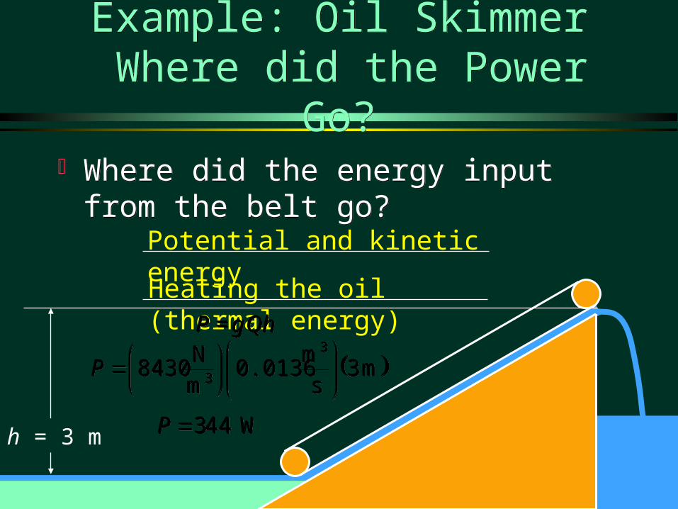
Potential and kinetic energy
Heating the oil (thermal energy)
Example: Oil Skimmer Where did the Power Go?
Example: Oil Skimmer Where did the Power Go?
Where did the energy input from the belt go?
Where did the energy input from the belt go?
h = 3 m
P Qhg=P Qhg=
m 3s
m0.0136
mN
84303
3
P m 3
sm
0.0136mN
84303
3
P
W443P W443P

Velocity ProfilesVelocity Profiles
-2
-1
0
1
2
3
0 0.0005 0.001 0.0015 0.002
y (m)
u (m
/s)
oil
water
2
2 x
y y ay dpu U g
a dxm m r
- æ ö= + +è ø
2
2 x
y y ay dpu U g
a dxm m r
- æ ö= + +è ø
Pressure gradients and gravity have the same effect.
In the absence of pressure gradients and gravity the velocity profile is ________linear
Example: No flowExample: No flow
Find the velocity of a vertical belt that is 5 mm from a stationary surface that will result in no flow of glycerin at 20°C (= 0.62 Ns/m2 and =12300 N/m3)
Find the velocity of a vertical belt that is 5 mm from a stationary surface that will result in no flow of glycerin at 20°C (= 0.62 Ns/m2 and =12300 N/m3)
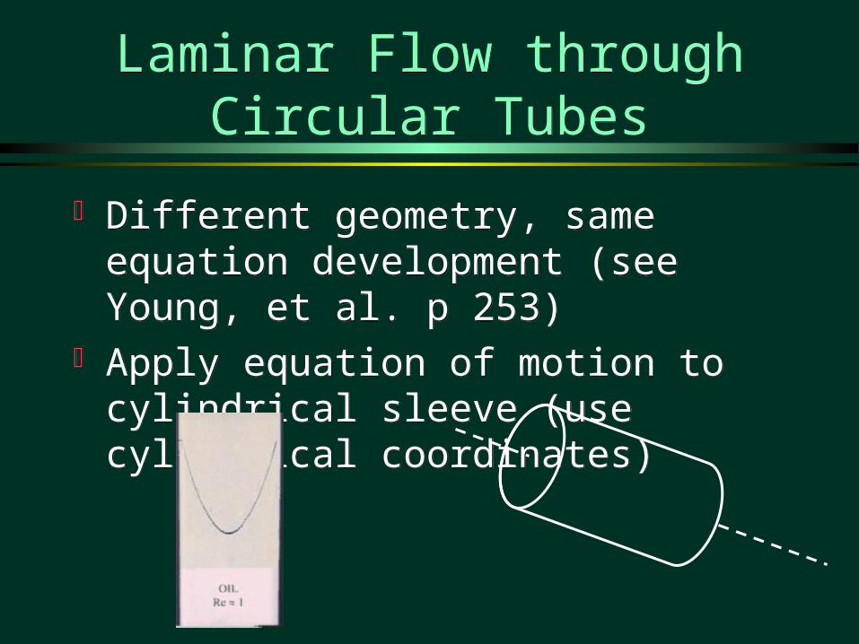
Laminar Flow through Circular Tubes
Laminar Flow through Circular Tubes
Different geometry, same equation development (see Young, et al. p 253)
Apply equation of motion to cylindrical sleeve (use cylindrical coordinates)
Different geometry, same equation development (see Young, et al. p 253)
Apply equation of motion to cylindrical sleeve (use cylindrical coordinates)
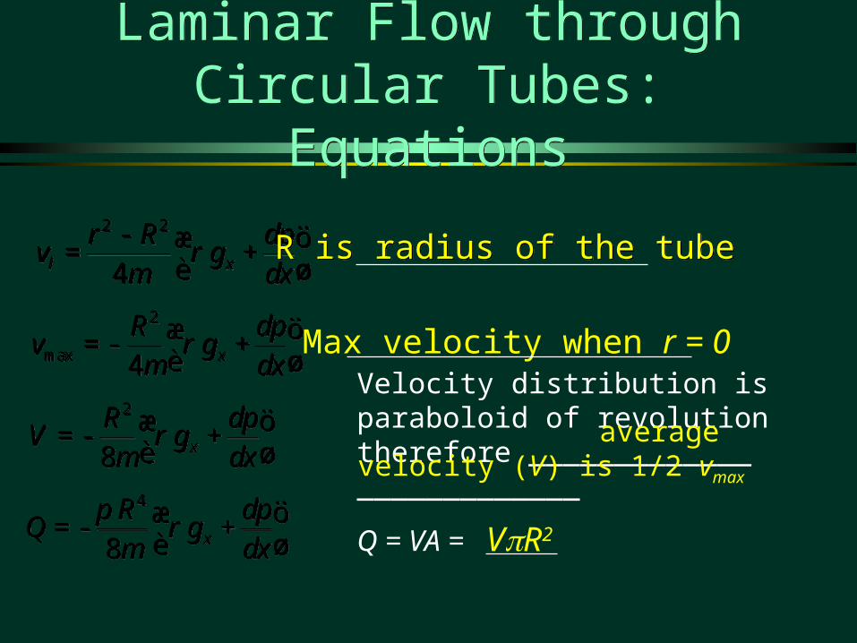
Max velocity when r = 0
Laminar Flow through Circular Tubes: Equations
Laminar Flow through Circular Tubes: Equations
2 2
4l x
r R dpv g
dxr
m- æ ö= +
è ø
2 2
4l x
r R dpv g
dxr
m- æ ö= +
è ø
2
max 4 x
R dpv g
dxr
mæ ö=- +è ø
2
max 4 x
R dpv g
dxr
mæ ö=- +è ø
2
8 x
R dpV g
dxr
mæ ö=- +è ø
2
8 x
R dpV g
dxr
mæ ö=- +è ø
4
8 x
R dpQ g
dxp
rmæ ö=- +è ø
4
8 x
R dpQ g
dxp
rmæ ö=- +è ø
Velocity distribution is paraboloid of revolution therefore _____________ _____________
Q = VA =
average velocity (V) is 1/2 vmax
VR2
R is radius of the tubeR is radius of the tube
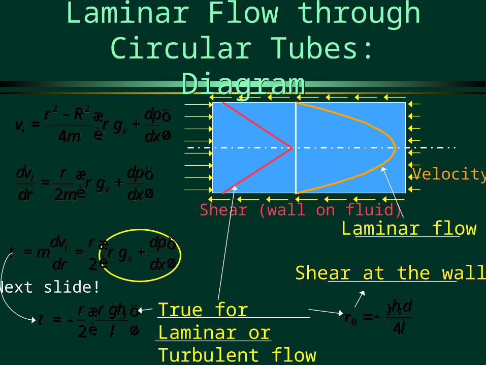
Laminar Flow through Circular Tubes: Diagram
Laminar Flow through Circular Tubes: Diagram
Velocity
Shear (wall on fluid)2
lx
dv r dpg
dr dxr
mæ ö= +è ø2
lx
dv r dpg
dr dxr
mæ ö= +è ø
2l
x
dv r dpg
dr dxt m ræ ö= = +
è ø2l
x
dv r dpg
dr dxt m ræ ö= = +
è ø
2lghr
lr
t æ ö=-è ø2
lghrl
rt æ ö=-
è ø l
dhl
40
l
dhl
40
True for Laminar or Turbulent flow
Shear at the wallShear at the wall
Laminar flow
2 2
4l x
r R dpv g
dxr
m- æ ö= +
è ø
2 2
4l x
r R dpv g
dxr
m- æ ö= +
è ø
Next slide!
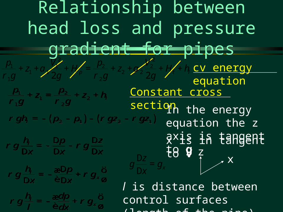
cv energy equation
Relationship between head loss and pressure gradient for pipesRelationship between head loss and pressure gradient for pipes
1 21 2
1 2l
p pz z h
g gr r+ = + +1 2
1 21 2
l
p pz z h
g gr r+ = + + Constant cross section
2 21 1 2 2
1 1 2 21 22 2p t l
p V p Vz H z H h
g g g ga a
r r+ + + = + + + +
( ) ( )2 1 2 1lgh p p gz gzr r r=- - - -( ) ( )2 1 2 1lgh p p gz gzr r r=- - - -
lh p zg g
x x xr r
D D=- -
D D Dlh p z
g gx x x
r rD D
=- -D D D
lx
h pg g
x xr r
Dæ ö=- +è øD D
lx
h pg g
x xr r
Dæ ö=- +è øD D
lx
h dpg g
l dxr ræ ö=- +
è øl
x
h dpg g
l dxr ræ ö=- +
è ø
l is distance between control surfaces (length of the pipe)
In the energy equation the z axis is tangent to g
x is in tangent to V
x
zg g
xD
=D
xz

The Hagen-Poiseuille EquationThe Hagen-Poiseuille Equation
4
128lhD
Ql
gpm
=4
128lhD
Ql
gpm
=2
32lhD
Vl
gm
=2
32lhD
Vl
gm
=
Hagen-Poiseuille Laminar pipe flow equations4
8 x
R dpQ g
dxp
rmæ ö=- +è ø
4
8 x
R dpQ g
dxp
rmæ ö=- +è ø
From Navier-Stokes
4
8lhR
Q gl
pr
mæ ö=- -è ø
4
8lhR
Q gl
pr
mæ ö=- -è ø
lx
h dpg g
l dxr ræ ö=- +
è øl
x
h dpg g
l dxr ræ ö=- +
è øRelationship between head loss and pressure gradient
What happens if you double the pressure gradient in a horizontal tube? ____________flow doubles
V is average velocity
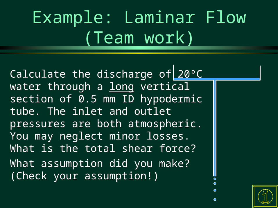
Example: Laminar Flow (Team work)
Example: Laminar Flow (Team work)
Calculate the discharge of 20ºCwater through a long vertical section of 0.5 mm ID hypodermic tube. The inlet and outlet pressures are both atmospheric. You may neglect minor losses. What is the total shear force?
What assumption did you make? (Check your assumption!)
Calculate the discharge of 20ºCwater through a long vertical section of 0.5 mm ID hypodermic tube. The inlet and outlet pressures are both atmospheric. You may neglect minor losses. What is the total shear force?
What assumption did you make? (Check your assumption!)
SummarySummary
Navier-Stokes Equations and the Continuity Equation describe complex flow including turbulence
The Navier-Stokes Equations can be solved analytically for several simple flows
Numerical solutions are required to describe turbulent flows
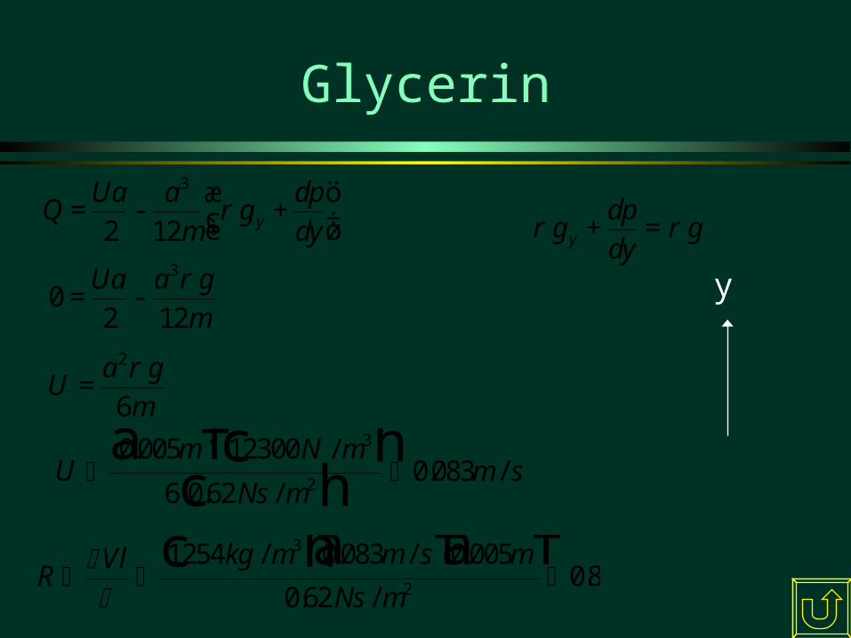
GlycerinGlycerin
3
2 12 y
Ua a dpQ g
dyr
mæ ö
= - +ç ÷è ø3
02 12
Ua a grm
= -
y
dpg g
dyr r+ =
2
6a g
Urm
=
Um N m
Ns mm s
0 005 12300
6 0 620 083
2 3
2
. /
. /. /
a fc hc h
RVl kg m m s m
Ns m
1254 0 083 0 005
0 620 8
3
2
/ . / .
. /.
c ha fa f
y
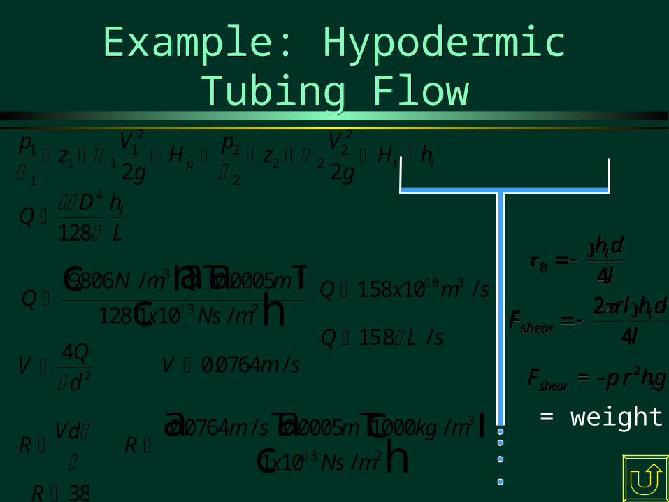
Example: Hypodermic Tubing Flow
Example: Hypodermic Tubing Flow
QD h
Ll
4
128
QN m m
x Ns m
9806 0 0005
128 1 10
3 4
3 2
/ .
/
c hafa fc h
Q x m s 158 10 8 3. /
VQd
4
2V m s 0 0764. /
RVd
Rm s m kg m
x Ns m
0 0764 0 0005 1000
1 10
3
3 2
. / . /
/
a fa fc hc h
R 38
Q L s 158. /
ldhl
40
ldhl
40
ldhrl
F lshear 4
2 l
dhrlF l
shear 42
2shear lF r hp g=- 2shear lF r hp g=-
= weight!
pz
Vg
Hp
zV
gH hp t l
1
11 1
12
2
22 2
22
2 2
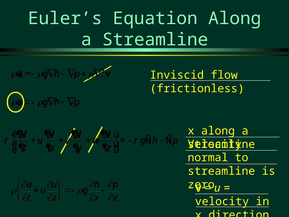
Euler’s Equation Along a Streamline
Euler’s Equation Along a Streamline
va 2 phg va 2 phg
xp
xh
gxu
utu
xp
xh
gxu
utu
phg a phg a
Inviscid flow (frictionless)
x along a streamline
v = u = velocity in x direction
Velocity normal to streamline is zero
u v w g h pt x y z
r r¶ ¶ ¶ ¶é ù
+ + + =- Ñ - Ñê ú¶ ¶ ¶ ¶ë û
V V V Vu v w g h p
t x y zr r¶ ¶ ¶ ¶é ù
+ + + =- Ñ - Ñê ú¶ ¶ ¶ ¶ë û
V V V V

Euler’s EquationEuler’s Equation
xp
xh
gxu
u
1
xp
xh
gxu
u
1
01
dxdp
dxdh
gdxdu
u
01
dxdp
dxdh
gdxdu
u
0 udugdhdp
0 udugdhdp
(Multiplying by dx converts from a force balance equation to an energy equation)
xp
xh
gxu
utu
xp
xh
gxu
utu
We’ve assumed: frictionless and along a streamline
SteadySteady
Euler’s equation along a streamline
x is the only independent variable

Bernoulli EquationBernoulli Equation
0 udugdhdp
0 udugdhdp
Euler’s equation
01 udugdhdp
01 udugdhdp
constant2
2
vgh
p
constant2
2
vgh
p
constant2
2
g
vh
p
constant2
2
g
vh
p
The Bernoulli Equation is a statement of the conservation of ____________________
constant2
2
vgh
p
constant2
2
vgh
p
Integrate for constant density
Bernoulli Equation
Mechanical Energy p.e. k.e.

Hydrostatic Normal to Streamlines?
Hydrostatic Normal to Streamlines?
phgz
wy
vx
ut
vvvvphg
zw
yv
xu
t
vvvv
xp
xh
gxu
utu
xp
xh
gxu
utu
y
p
y
hg
0y
p
y
hg
0 dhdp dhdp
y
p
y
hg
z
vw
y
vv
x
vu
t
v
y
p
y
hg
z
vw
y
vv
x
vu
t
v
y, v perpendicular to streamline (v = 0)
x, u along streamline
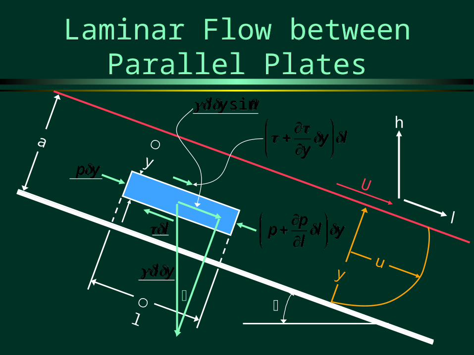
Laminar Flow between Parallel Plates
Laminar Flow between Parallel Plates
U
l
a
uy
lyy
lyy
yllp
p
yl
lp
p
ypyp
ll
yl yl
sinyl sinyl
y
h
l
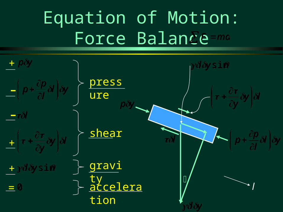
Equation of Motion: Force Balance
Equation of Motion: Force Balance
lyy
lyy
yllp
p
yl
lp
p
ypyp
ll
yl yl
sinyl sinyl
ypyp
yllp
p
yl
lp
p
ll
lyy
lyy
maF maF
sinyl sinyl
00
pressure
shear
gravity
acceleration
+
-
-
+
+
= l
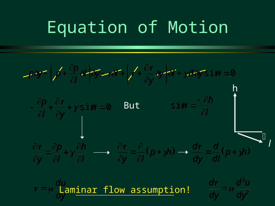
Equation of MotionEquation of Motion
0sin
ylp
0sin
ylp
lh
sinlh
sin
lh
lp
y
lh
lp
y
hp
ly
hp
ly
hp
dld
dyd hp
dld
dyd
dydu dydu 2
2
dyud
dyd 2
2
dyud
dyd
But
h
l
Laminar flow assumption!Laminar flow assumption!
0sin
ylly
ylyl
lp
pyp 0sin
ylly
ylyl
lp
pyp
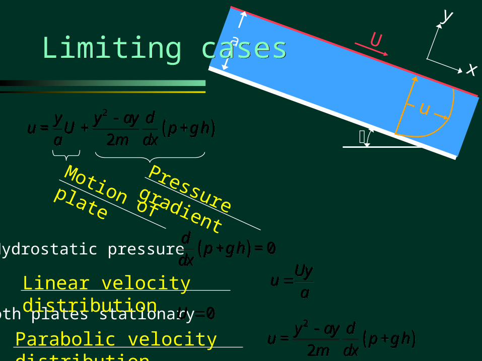
U
a
u
Limiting casesLimiting cases
( )2
2y y ay d
u U p ha dx
gm-
= + +( )2
2y y ay d
u U p ha dx
gm-
= + +
Both plates stationary
Hydrostatic pressure ( ) 0d
p hdx
g+ =( ) 0d
p hdx
g+ =
aUy
u a
Uyu
0U 0U
( )2
2y ay d
u p hdx
gm-
= +( )2
2y ay d
u p hdx
gm-
= +
Linear velocity distribution
Parabolic velocity distribution
Motion of plate
Pressure gradient
y
x
Related Documents